Sampling from a Finite Population: IntervalEstimation of Means, Proportions and Population

Totals

Jerry Brunner

March 21, 2007

Most of the material in this course is based on the assumption that we are samplingwith replacement, or else sampling without replacement from an “infinite population”(definitely a theoretical abstraction. We have justified this on the grounds of simplicity,and also because if the population is very large, there is very little difference betweensampling with and without replacement.

But in practice, sampling is almost always without replacement. Furthermore, wecan use information about the size of the population (and sometimes the sizes of sub-populations) to estimate population totals, and to make the estimation of means andpercentages more precise. Precision of estimation is usually purchased by increasingsample size, and data collection costs money. If you can design a survey so as to getprecise estimation some other way, you can use a smaller sample and save money.

1 Simple random sampling without replacement

Suppose we select a random sample of size n without replacement from a population of sizeN . Imagine putting a N balls in a jar; each ball is labelled with the identification numberof one member of the population. You pull out n balls without looking (and withoutreplacement), record the numbers, and collect data from the corresponding members ofthe population. the population mean is µ, and the population standard deviation is σ.

Each subset of the population will have an equal chance of being chosen, and eachindividual in the population will have an equal chance of being in the sample. Of coursein practice you would not use a big jar of balls; you’d model the process of selection on acomputer, using a stream of pseudo-random numbers from a random number generator.

1.1 Estimating means

When you randomly sample n units without replacement from a population of size N ,

• The point estimate of the population mean µ is still the sample mean x.

1

• x is still unbiased for µ. That is, the expected value of the sampling distribution ofx is µ.

• The standard error of the mean (standard deviation of the sampling distribution of

x) is σx = σ√n

√1− n

N. We never know σ, but for n ≥ 30 we can estimate it with

the sample standard deviation s, and estimate σx with

σ̂x =s√n

√1− n

N(1)

• The Central Limit Theorem still applies. We will assume n ≥ 30, with a differentrule when the population mean is actually a proportion.

Notice that when you are sampling with replacement, the standard error of the mean isσ√n, but when you are sampling without replacement, the standard error of the mean is σ√

n

multiplied by√

1− nN

. The quantity√

1− nN

is called the finite population correction

factor.

• The finite population correction factor is always less than one. This means thatwhen you sample without replacement, estimation of the population mean is a littlemore precise; the margin of error is a bit smaller, and the confidence interval is abit narrower.

• If n = N , the finite population correction factor equals zero, and so does σx. Thismakes sense. If you sample the whole population, there is no error of estimation.

Consider a population with true standard deviation σ = 6. We estimate µ with thesample mean x, based on a random sample of size n without replacement from a populationof size N . Table 1.1 shows the standard error of the mean σx for various values of n andN . Bear in mind that σx represents the variation of x around the population mean, sosmaller values of σx mean more precise estimation.

Notice that once the population is reasonably large, σx barely changes as the popula-tion size gets larger, while it goes down rapidly with increasing sample size. The moralis that except for very small populations, what matters is the size of the sample, not thesize of the population.

The Central Limit Theorem for finite populations says that for large samples,

Z =x− µ

s√n

√1− n

N

is approximately standard normal; we will apply it when n ≥ 30. This leads to theestimated (1− α)100% margin of error

zα/2s√n

√1− n

N(2)

and the (1− α)100% confidence interval for µ

x± zα/2s√n

√1− n

N(3)

2

Table 1: Standard error of the mean σx, sampling n observations without replacementfrom a population of size N : Population standard deviation is σ = 20

nN 25 50 100 500 1,00050 2.8284 0.0000100 3.4641 2.0000 0.0000500 3.8987 2.6833 1.7889 0.0000

1,000 3.9497 2.7568 1.8974 0.6325 0.000010,000 3.9950 2.8213 1.9900 0.8718 0.6000100,000 3.9995 2.8277 1.9990 0.8922 0.6293

1,000,000,000 4.0000 2.8284 2.0000 0.8944 0.632510,000,000,000 4.0000 2.8284 2.0000 0.8944 0.6325100,000,000,000 4.0000 2.8284 2.0000 0.8944 0.6325

1.2 Estimating proportions and percentages

Suppose the data x1, . . . , xn are coded so that xi = 1 if the event (the customer buys theproduct, the shipment arrives on time, etc.) happens for observation i, and xi = 0 if itdoes not happen. Then

• The population mean is µ = p, the population proportion.

• The sample mean is x = p̂, the sample proportion

• The population standard deviation is σ =√

p(1− p), but we never know it, so we

use the estimate√

p̂(1− p̂).

• The estimated standard deviation of the sample proportion is

σ̂p̂ =

√p̂(1− p̂)

n

√1− n

N. (4)

• The Central Limit Theorem applies directly, because we are really dealing with asample mean. For large samples, Z = (p̂− p)/σ̂p̂ is approximately standard normal.

• Because we have binary data, we don’t use the n ≥ 30 rule. Instead, we checkwhether p̂± 3σ̂p̂ is inside the interval from zero to one.

The estimated (1− α)100% margin of error for p̂ as an estimate of p is

zα/2

√p̂(1− p̂)

n

√1− n

N(5)

3

and the (1− α)100% confidence interval for p is

p̂± zα/2

√p̂(1− p̂)

n

√1− n

N. (6)

To obtain a margin of error or confidence interval for a percentage, just multiplyeverything by 100. That is, the estimated (1 − α)100% margin of error for the samplepercentage as an estimate of the population percentage is

100× zα/2

√p̂(1− p̂)

n

√1− n

N(7)

and the (1− α)100% confidence interval for p is

100× p̂± 100× zα/2

√p̂(1− p̂)

n

√1− n

N. (8)

1.3 Estimating population totals

Since

µ =1

N

N∑i=1

xi,

the population total∑N

i=1 xi = Nµ, and we estimate it with Nx. This applies whetherdata are binary or not. If the data are zeros and ones, the population total is the totalnumber of something, like the total number of cable TV subscribers in Canada. If thedata represent amount of something, the population total is total amount, like the totalamount of money spent on fast food in Ontario during the past month. If the data aresomething like ratings of customer satisfaction, the population mean is of interest, butthe population total is meaningless.

Using the symbol x instead of p̂ if the data happen to be zeros and ones, the (1−α)100%margin of error for the estimated population total is

Nzα/2σ̂x (9)

and the (1− α)100% confidence interval for the population total is

Nx±Nzα/2σ̂x, (10)

where again, if the data are 1=Yes and 0=No, then x = p̂, and σ̂x is given by (16).Otherwise, σ̂x is given by (1).

Example 1.1 The United States is divided into 3078 districts (counties or county equiva-lents). We randomly sample 300 of these without replacement, and determine the numberof acres devoted to farms. The sample mean number of farm acres is 297.9 thousand,with a standard deviation of 344.6 thousand. Give a point estimate and a 95% margin oferror for the total number of acres devoted to farms in the U. S.

4

Exercises

1. We select a random sample of 300 without replacement from a population of size450. What is the finite population correction factor? The answer is a number.

2. From a campus with 4250 students, we select a random sample of size 200 withoutreplacement, and ask if they have broadband Internet access at home; 145 say Yes.

(a) Give a 95% confidence interval for the population proportion of students whoclaim to have Internet access at home.

(b) Give a 95% confidence interval for the true percentage of students who claimto have Internet access at home.

(c) Give a point estimate and a 95% confidence interval for the true total numberof students who claim to have Internet access at home.

(d) How do you know that the sample size is large enough to do what you havedone? Show your work.

3. There are 31,989 homes in Stephens County, a rural area in Manitoba. We selecta simple random sample of 500 homes without replacement, and check their as-sessed value from county records. We get a sample mean of $69,368 and a standarddeviation of $16,456.

(a) Give a 95% confidence interval for the population mean assessed value of homesin Stephens County.

(b) Give a point estimate and a 95% confidence interval for the true total assessedvalue of homes in Stephens County.

(c) How do you know that the sample size is large enough to do what you havedone?

2 Stratified random sampling

In stratified random sampling, the population is divided into segments, or strata. Thesizes of the strata are known, usually from census data. Then you select a probabilitysample (in our case, a simple random sample without replacement) from each stratum,with the objective of estimating population means, percentages and totals.

Why would you stratify? If estimates within strata are of interest (like estimatingthe mean time playing video games in each province), stratification can ensure that youhave enough data from each stratum to do a reasonable analysis. To accomplish this,it is common to deliberately over-sample from smaller strata. Another advantage ofstratification is that it can increase precision when you are estimating parameters of thewhole population – provided the variable you are interested in is substantially differentfrom stratum to stratum. For example, if you were interested in estimating the averagehours of sports watched by students on a campus, it would be natural to stratify by sex.

5

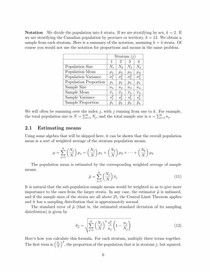
Notation We divide the population into k strata. If we are stratifying by sex, k = 2. Ifwe are stratifying the Canadian population by province or territory, k = 13. We obtain asample from each stratum. Here is a summary of the notation, assuming k = 4 strata. Ofcourse you would not use the notation for proportions and means in the same problem.

Stratum (j)1 2 3 4

Population Size N1 N2 N3 N4

Population Mean µ1 µ2 µ3 µ4

Population Variance σ21 σ2

2 σ23 σ2

4

Population Proportion p1 p2 p3 p4

Sample Size n1 n2 n3 n4

Sample Mean x1 x2 x3 x4

Sample Variance s21 s2

2 s23 s2

4

Sample Proportion p̂1 p̂2 p̂3 p̂4

We will often be summing over the index j, with j running from one to k. For example,the total population size is N =

∑ki=1 Nj, and the total sample size is n =

∑ki=1 nj.

2.1 Estimating means

Using some algebra that will be skipped here, it can be shown that the overall populationmean is a sort of weighted average of the stratum population means.

µ =k∑

j=1

(Nj

N

)µj =

(N1

N

)µ1 +

(N2

N

)µ2 + · · ·+

(Nk

N

)µk

The population mean is estimated by the corresponding weighted average of samplemeans.

µ̂ =k∑

j=1

(Nj

N

)xj (11)

It is natural that the sub-population sample means would be weighted so as to give moreimportance to the ones from the larger strata. In any case, the estimator µ̂ is unbiased,and if the sample sizes of the strata are all above 25, the Central Limit Theorem appliesand it has a sampling distribution that is approximately normal.

The standard error of µ̂ (that is, the estimated standard deviation of its samplingdistribution) is given by

σ̂µ̂ =

√√√√√ k∑j=1

(Nj

N

)2 s2j

nj

(1− nj

Nj

)(12)

Here’s how you calculate this formula. For each stratum, multiply three terms together.

The first term is(

Nj

N

)2, the proportion of the population that is in stratum j, but squared.

6

The second term iss2j

nj, the standard error of the sample mean for stratum j, but squared.

The third term is(1− nj

Nj

), the finite population correction factor, but squared.

After taking the product of these three terms for each stratum, you add up the prod-ucts. Then you take the square root of the sum.

Once you have the standard error, it’s easy to calculate the

(1− α)100% Margin of Error = zα/2σ̂µ̂, (13)

and the confidence interval is µ̂ plus or minus the margin of error. That is,

µ̂± zα/2σ̂µ̂. (14)

Here is an example with two strata. On a quiz or the exam, you might be asked for apoint estimate of µ if there are more than two strata, but a margin of error would requiretoo much time. To calculate a margin of error for a problem with more than two strata,you need Excel or something like that; expect it as a computer assignment.

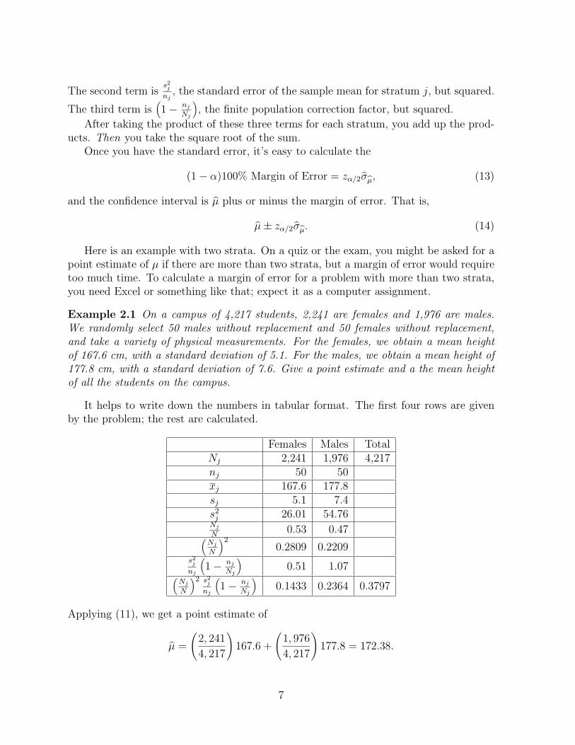
Example 2.1 On a campus of 4,217 students, 2,241 are females and 1,976 are males.We randomly select 50 males without replacement and 50 females without replacement,and take a variety of physical measurements. For the females, we obtain a mean heightof 167.6 cm, with a standard deviation of 5.1. For the males, we obtain a mean height of177.8 cm, with a standard deviation of 7.6. Give a point estimate and a the mean heightof all the students on the campus.

It helps to write down the numbers in tabular format. The first four rows are givenby the problem; the rest are calculated.

Females Males TotalNj 2,241 1,976 4,217nj 50 50xj 167.6 177.8sj 5.1 7.4s2

j 26.01 54.76Nj

N0.53 0.47(

Nj

N

)20.2809 0.2209

s2j

nj

(1− nj

Nj

)0.51 1.07(

Nj

N

)2 s2j

nj

(1− nj

Nj

)0.1433 0.2364 0.3797

Applying (11), we get a point estimate of

µ̂ =

(2, 241

4, 217

)167.6 +

(1, 976

4, 217

)177.8 = 172.38.

7

The last row has the products we need for the estimated standard error of µ̂, and thelower right-hand cell has the sum of products. All we need to do now is take the squareroot, and

σ̂µ̂ =√

0.3797 = 0.616.

The 95% margin of error is now zα/2σ̂µ̂ = (1.96)(0.616) = 1.21, and the 95% confidenceinterval is µ̂± zα/2σ̂µ̂ = 172.38± 1.21, or the interval from 171.17cm to 173.59cm.

2.2 Estimating proportions and percentages

The formulas we need are closely parallel to the ones from the preceding section. Thepoint estimate of a population proportion is

p̂ =k∑

j=1

(Nj

N

)p̂j, (15)

with standard error

σ̂p̂ =

√√√√√ k∑j=1

(Nj

N

)2 p̂j(1− p̂j)

nj

(1− nj

Nj

)(16)

To use the normal distribution to get a margin of error, we need p̂± 3σ̂p̂ to be inside theinterval from zero to one. To estimate percentages, multiply the following by 100: thepoint estimate, the margin of error, and the endpoints of the confidence interval.

Example 2.2 We take independent random samples without replacement from each ofthe Canadian Provinces and Territories. Among other things, we ask education. Figure 1below shows the calculations needed to estimate the proportion of Canadians who finisheduniversity. This is a printout of the Excel spreadsheet ugrad.xls, which is availableonline.

Of some interest is zα/2; it definitely did not come from a table. The code is=NORMINV(1-D19/2,0,1). You give the NORMINV function a number (call it a), and itgives you the value x such that the area under the normal curve less than or equal to x isequal to a. The second and third arguments of the function are the mean and standarddeviation of the normal distribution you want. I asked for a standard normal distributionby specifying 0 and 1. The first argument is 1−α/2, where α = 0.05 is in D19. If I changethe value in D19, say to 0.01, the margin of error and the confidence interval updateinstantly. It’s very nice.

2.3 Estimating population totals

As in the case of a single random sample, population totals are estimated by multiplyinga sample proportion or sample mean by the population size. If the data are zeros and

8

Figure 1: Spreadsheet for Estimating Proportion of Canadians with University Educations

Pop Size Sample Size Prop U Grad

Nj nj Nj /N Product

Newfoundland and Labrador 519,400 100 0.14 0.01655601 0.00231784 0.00027 0.001204 0.99980747 3.29954E-07

Prince Edward Island 136,900 100 0.17 0.00436372 0.00074183 1.9E-05 0.001411 0.99926954 2.68487E-08

Nova Scotia 934,500 100 0.2 0.02978742 0.00595748 0.00089 0.0016 0.99989299 1.41951E-06

New Brunswick 750,300 100 0.16 0.023916 0.00382656 0.00057 0.001344 0.99986672 7.68632E-07

Quebec 7,445,700 200 0.22 0.23733357 0.05221339 0.05633 0.000858 0.99997314 4.83275E-05

Ontario 12,102,000 200 0.25 0.38575431 0.09643858 0.14881 0.0009375 0.99998347 0.000139504

Manitoba 1,155,600 100 0.2 0.03683504 0.00736701 0.00136 0.0016 0.99991346 2.17072E-06

Saskatchewan 995,900 100 0.18 0.03174456 0.00571402 0.00101 0.001476 0.99989959 1.48724E-06

Alberta 3,116,300 100 0.21 0.09933285 0.0208599 0.00987 0.001659 0.99996791 1.63689E-05

British Columbia 4,115,400 100 0.24 0.13117942 0.03148306 0.01721 0.001824 0.9999757 3.13867E-05

Yukon Territory 30,100 100 0.23 0.00095945 0.00022067 9.2E-07 0.001771 0.99667774 1.62485E-09

Northwest Territories 41,500 100 0.19 0.00132282 0.00025134 1.7E-06 0.001539 0.99759036 2.68655E-09

Nunavut 28,700 100 0.12 0.00091482 0.00010978 8.4E-07 0.001056 0.99651568 8.80682E-10

Total 31,372,300 1,500 1 0.22750146 0.000241795

! 0.05

z!/2 1.95996398

0.228

0.01554975

Margin of Er 0.030

Lower CL 0.197

Upper CL 0.258

0.181

0.274

!

jˆ p

!

N j

N

"

# $

%

& ' ̂ p j

!

N j

N

"

# $

%

& '

2

!

ˆ p j (1" ˆ p j )

n j

!

N j " n j

N j

!

ˆ p ˆ "

!

ˆ p

!

ˆ p ˆ p "3 ˆ #

!

ˆ p ˆ p +3 ˆ "

ones, the population total is the total number of something. For example, one mightdivide the city of Toronto into little square regions, take a random sample of regions, andestimate the mean number of under-the-table “cash only” plumbers in each one. Thisestimate would be multiplied by the total number of regions to estimate the total numberof unregistered plumbers in Toronto.

If the data consist of amount of something, the population total is total amount.For example, suppose we could estimate the mean amount of gasoline in the gas tanksof vehicles registered in Ontario, and then multiply by the total number of vehicles toestimate the total litres of gas in this unpublicized “strategic reserve.”

To estimate population totals, start with either estimation of a proportion or a moregeneral mean, and then multiply the following by 100: the point estimate, the margin oferror, and the endpoints of the confidence interval. There; we did it without any formulas.

Example 2.3 Continuing Example 2.2, give a point estimate and a 95% margin of errorfor the total number of university graduates in Canada.

The point estimate is t̂ = Np̂ = (31, 372, 300)(0.228) = 7, 152, 884 university gradu-ates. The margin of error is N times the 95% margin of error for the proportion. That’s(31, 372, 300)(0.030) = 941, 169.

9

That was easy, but the moral of the story is serious. That margin of error is large!We are comfortable with our estimate give or take almost a million people. It’s not veryimpressive, but that’s how it goes with the estimation of totals. You multiply a smallmargin of error by a very big number, and you get a big number. The estimation of totalsis inherently not very precise. This is all the more reason to provide a margin of erroralong with any estimate.

Example 2.4 Managers of a cable TV company want to know the number of satellitedishes in a large city. They have high-resolution photographs of the city from the air.They divide the city into square regions of equal area. With enough patience, it is possibleto count the number of dishes in one of the squares using a magnifying glass, but it istoo expensive to hire people to do it all, or to divert enough current employees from theirduties to d the job. Accordingly, management decide to estimate the quantity they want.

The city is divided into six regions (strata) based on average building height, yard size,residential/commercial mix, and so on. Then a random sample of squares is selected fromeach region, and the number of dishes in each square is counted from aerial photographs.The data are in the spreadsheet TotalDishes.xls (See Figure 2; it’s also posted online.)Give a point estimate and a 95% margin of error for the total number of satellite dishes.

Figure 2: Spreadsheet for Estimating Total Number of Satellite Dishes

Stratum (j) Nj nj DxF HxIxJ1 400 98 24.1 5,575 0.5722 13.791 0.32747 56.8877551 0.755 14.064732 30 10 25.6 4,064 0.0429 1.0987 0.00184 406.4 0.66667 0.4990583 61 37 267.6 347,556 0.0873 23.353 0.00762 9393.40541 0.39344 28.145554 18 6 179 22,789 0.0258 4.6094 0.00066 3798.16667 0.66667 1.6790885 70 39 293.7 123,578 0.1001 29.412 0.01003 3168.66667 0.44286 14.072856 120 21 33.2 9,795 0.1717 5.6996 0.02947 466.428571 0.825 11.34089

Total 699 1 77.964 69.8022

77.964

8.3548

54,497

5840

0.05

1.96Margin of Err 11,446

!

j

2

s

!

jx

!

N j

N

"

# $

%

& '

!

N j " n j

N j

!

N j

N

"

# $

%

& '

2

!

s j2

n j

!

ˆ µ

!

ˆ t =N ˆ µ

!

ˆ t ˆ " = N ˆ µ ˆ " !

ˆ µ ˆ "

!

"

!

" /2z

10

We end up with an estimate of 54,497 dishes, with a 95% margin of error equal to11,446. Again, estimation of totals is not very precise. That does not mean one shouldn’tdo it, but it’s very important to be aware of the margin of error.

Exercises

1. The following table shows Census data for number of people employed, along withsample means from a stratified random sample, where the strata were Provinces orTerritories. Give a point estimate of the mean annual income in Canada (in 2001).The answer is a single number.

Province or Number people employed Sample mean

Territory (Census) reported earnins

Newfoundland 251,545 $24,165

P.E.I. 77,750 $22,303

Nova Scotia 468,825 $26,632

New Brunswick 388,855 $24,971

Quebec 3,815,265 $29,385

Ontario 6,319,530 $35,185

Manitoba 609,575 $27,178

Saskatchewan 534,350 $25,691

Alberta 1,768,435 $32,603

Brit. Columbia 2,128,550 $31,544

Yukon 18,780 $31,526

N.W.T 21,955 $36,645

Nunavut 12,355 $28,215

TOTAL 16,415,785

2. The United States is divided into four large census regions: Northeast, North Cen-tral, South, and West. A random sample of 250 individuals in the labour force wereselected from each region. The table below shows percentages unemployed.

Region Civilian Labour Force (in thousands) Sample Percent UnemployedNortheast 27,870.8 4.7%North Central 34,626.9 5.1South 53,397.5 4.6West 34,453.0 4.8

In the calculations that follow, you can omit the finite population correction factorsif you wish, because they are so close to one. It won’t affect the results.

11

(a) Give a point estimate of the percent (not proportion) of unemployed personsin the U.S. labour force. The answer is a single number.

(b) Is the sample size big enough to get a margin of error? Answer Yes or No andshow your work.

(c) Give the 95% margin of error for the percent unemployed. The answer is asingle number.

(d) Give a point estimate of the total number of unemployed persons in the U.S.labour force. The answer is a single number.

(e) Give the 95% margin of error for the total number unemployed. The answer isa single number.

3. Naturally, the U.S. insurance industry is very interested in how long people stay inhospital. They want the stays to be as short (and therefore presumably inexpensive)as possible. For the four large census regions in the US, there are (or were, in 1994)902 hospitals in the Northeast, 1,704 in the North Central, 2,291 in the South,and 1,126 in the West. A random sample was selected from each region withoutreplacement, and average length of stay was determined from hospital records. Thesurvey was in 1994 too. Results are given in the table below.

Analysis Variable : stay Av length of hospital stay, in days

Region of N

country (usa) Obs Mean Std Dev

----------------------------------------------------

Northeast 30 11.0565517 2.6273021

North Central 50 9.6834375 1.1929378

South 50 9.1647222 1.2314556

West 30 8.1137500 1.0031210

----------------------------------------------------

Give a point estimate and a 95% margin of error for the population mean length ofstay for U.S. hospitals in 1994.

3 Quota samples

A quota sample is a stratified but non-probability sample. That is, the population isdivided into strata, and then a sample is obtained – somehow – within each stratum. Lotsof quota sample come from panel studies, in which a large group of consumers are recruitedto fill out surveys on an on-going basis, usually in exchange for very modest payment in

12

the form of coupons or free samples. The panels are usually described as “nationallyrepresentative,” meaning the proportions in various age, sex and maybe income groups isclose to census figures for the U. S. or Canadian population.

In quota samples, whether they come from a panel study or not, sample proportionsare usually selected to correspond to population proportions (but now always). Invari-ably, such samples are described as “representative.” You should be aware that the term“representative sample” is not a technical term from Statistics. It is a marketing term.Someone is trying to sell you data, probably data from a quota sample. Information froma quota sample may be better than unaided intuition, or it may be worse. There is nosure way to tell. For sure, regardless of their age and sex and even regardless of theireducation, members of a consumer panel are likely to be more literate than average. Afterall, they are willing to fill out a large number of questionnaires (in English), so it is prob-ably not too difficult for them. The market for books and similar products is consistentlyover-estimated by panel studies. On the other hand, the market for anti-psychotic drugsis probably under-estimated. Other topics? It’s largely guesswork.

Even so, if management decide to take data from quota samples seriously, it is a goodidea to apply the methods from this course, and to accompany all estimates with 95%margins of error. At least that way the decision-makers are reminded that the data yieldestimates, not absolute truth.

If you have data from a quota sample, and the sample sizes are proportional to thepopulation sizes, it is safe to use methods for a simple random sample, because then theconfidence intervals will be a little wider and the tests (when we get to them) will be a bitconservative, but that’s okay; no harm is done. If the sample sizes are not proportionalto the population sizes, treat it as a stratified random sample, using the methods fromthis chapter.

13