Adams JL, Schonlau M, Escarce J, Kilgore M, Schoenbaum M, Goldman DP. Sampling Patients Within and Across Health Care Providers: Multi-Stage Non-nested Samples in Health Services Research. Health Services and Outcomes Research Methodology. 2003; 4(3): 151-167. Sampling Patients Within and Across Health Care Providers: Multi-Stage

Non-nested Samples in Health Services Research

John L. Adams, Matthias Schonlau, José J. Escarce,

Meredith Kilgore, Michael Schoenbaum, Dana P. Goldman

RAND Abstract

In order to better inform study design decisions when sampling patients within and across

health care providers we develop a simulation-based approach for designing complex multi-stage

samples. The approach explores the tradeoff between competing design goals such as precision

of estimates, coverage of the target population and cost.

We elicit a number of sensible candidate designs, evaluate these designs with respect to

multiple sampling goals, investigate their tradeoffs, and identify the design that is the best

compromise among all goals. This approach recognizes that, in the practice of sampling,

precision of the estimates is not the only important goal, and that there are tradeoffs with

coverage and cost that should be explicitly considered. One can easily add other goals. We

construct a sample frame with all phase III clinical cancer treatment trials that are conducted by

cooperative oncology groups of the National Cancer Institute from October 1, 1998 through

December 31, 1999. Simulation results for our study suggest sampling a different number of

trials and institutions than initially considered.

1

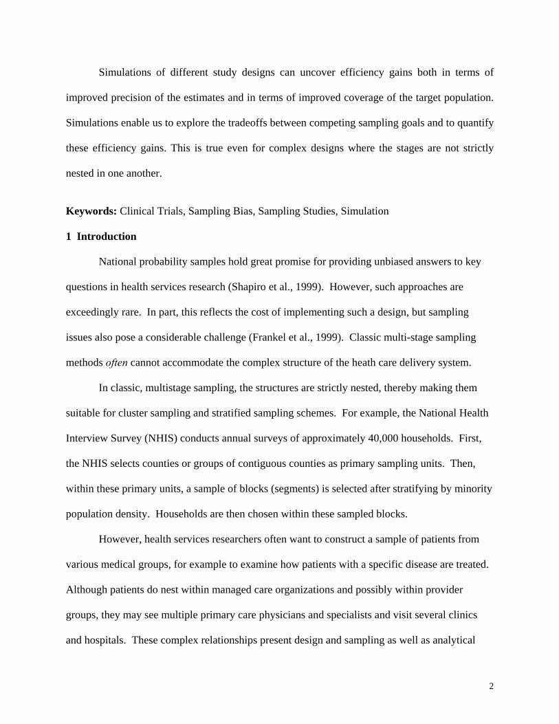
Simulations of different study designs can uncover efficiency gains both in terms of

improved precision of the estimates and in terms of improved coverage of the target population.

Simulations enable us to explore the tradeoffs between competing sampling goals and to quantify

these efficiency gains. This is true even for complex designs where the stages are not strictly

nested in one another.

Keywords: Clinical Trials, Sampling Bias, Sampling Studies, Simulation

1 Introduction

National probability samples hold great promise for providing unbiased answers to key

questions in health services research (Shapiro et al., 1999). However, such approaches are

exceedingly rare. In part, this reflects the cost of implementing such a design, but sampling

issues also pose a considerable challenge (Frankel et al., 1999). Classic multi-stage sampling

methods often cannot accommodate the complex structure of the heath care delivery system.

In classic, multistage sampling, the structures are strictly nested, thereby making them

suitable for cluster sampling and stratified sampling schemes. For example, the National Health

Interview Survey (NHIS) conducts annual surveys of approximately 40,000 households. First,

the NHIS selects counties or groups of contiguous counties as primary sampling units. Then,

within these primary units, a sample of blocks (segments) is selected after stratifying by minority

population density. Households are then chosen within these sampled blocks.

However, health services researchers often want to construct a sample of patients from

various medical groups, for example to examine how patients with a specific disease are treated.

Although patients do nest within managed care organizations and possibly within provider

groups, they may see multiple primary care physicians and specialists and visit several clinics

and hospitals. These complex relationships present design and sampling as well as analytical

2

challenges. Frequently these complex structures are forced into nested designs even though they

are inherently not nested.

This paper introduces a sampling methodology for multi-stage sampling of health service

users. The approach described here can be applied to any complex sampling problem where the

levels of the structure are not strictly nested. We consider all design alternatives that are thought

to be of interest, including sampling with equal probability and proportional to size as special

cases. Further, we explore alternative definitions of size. We consider different design goals and

use simulations to evaluate them and make the tradeoff between the competing goals explicit.

2 Background

The primary goals for study design should be to maximize the analytical information

while controlling data collection costs. The example above is instructive. The naïve approach

might be to sample patients at random and then go to all of their providers to review medical

records for patient characteristics and care received. This approach can result in “snowballing”

data collection costs as abstracters go from office to office to find the required charts. To keep

costs down, the design should capitalize on the lower marginal costs of data collection at

providers already being visited. Care must be taken, however, to ensure that the sample does not

end up concentrated only in the high volume providers or over-clustered in a way that hurts the

effective sample size.

A similar situation arises in other health services research contexts. The Cost of Cancer

Treatment Study (CCTS) was designed to measure the incremental costs of care in cancer

clinical trials (Goldman et al., 2000). The issue of how to pay for clinical care for patients in

cancer trials has received much attention recently. Most insurers or plans have policies that

exclude coverage for services given as part of a clinical trial (Mansour, 1994, Morrow et al.

3

1994, Wagner et al., 1999). The CCTS was conceived to provide precise, generalizable

estimates of the cost of conducting government-sponsored cancer trials.

To reach patients who are enrolled in clinical trials for cancer, it needed to address two

levels of organizational structure: clinical trials and institutions. Institutions are not strictly

nested within clinical trials, because many institutions participate in more than one trial. Most

trials are multisite and not nested within institution. An important feature of this problem is that

the cost of data collection is dominated by the fixed costs of adding another trial or institution to

the study, rather than the variable cost of adding patients within a trial-institution pair. Classical,

multi-stage sampling suggests three potential sampling schemes, each with its own problems.

A typical multi-stage sampling scheme would first sample trials proportional to size, and

then select institutions at which a trial is conducted with equal probability in a second stage.

(Kish, 1965, Chapter 7). We assume a complete listing of trial-institution pairs. Variations on

this approach include sampling with equal probability in both stages, or equal probability in the

first stage and proportional to size at the second stage (Kish, 1965). However, these approaches

ignore that it is more economical to sample an institution that has already been sampled for

another trial than one that has not been sampled yet. Consequently, typical designs are likely to

sample more institutions than would be cost efficient.

Another approach might be to list all possible pairs of trial-institution pairs and to sample

with equal probability or proportional to size. This approach also ignores potential economies

and will result in a sample that is spread across too many trial-institution pairs. A third

possibility might be to sample a fixed number of trials with equal probability or proportional to

size and sample all institutions at which these trials are conducted. If total costs are fixed, this is

4

likely to result in a design that has too few trials relative to the number of institutions sampled.

This is inefficient compared to alternative designs.

As our examples suggest, complex designs often have different competing goals.

Statisticians consider small design effects (the design effect specifies the loss or the gain in

precision of a design relative to simple random sampling), low or fixed cost, and small frame

error (e.g., due to ignoring very small trials and institutions) of the study as worthy design goals.

Sampling proportional to size might best support one goal of the study, whereas another goal

might be best supported by equal probability sampling.

Classical texts (Cochran, 1997) emphasize that it is important that the sampling frame

cover the target population well, but then focus on the tradeoff between cost and precision. The

tradeoff between precision and coverage (sampling units with non-zero chance of being sampled)

can be viewed as a tradeoff between variance and bias. This tradeoff is not usually explicitly

considered. Instead one usually focuses on the mean squared error, which specifies one specific

tradeoff between bias and variance. The “Total Survey Design” approach (Anderson et al., 1979,

Linacre et al., 1993) aims to design surveys such that the total error, a generalization of the mean

squared error, is minimized given a fixed cost constraint. For this approach to work, various bias

components, including the one stemming from a lack of coverage, need to be modeled explicitly.

This requires either additional auxiliary data sources or can be accomplished by conducting an

evaluation survey prior to the actual survey. The mean squared error of a variable of interest y is

defined as

MSE(y) = Var(y) + Bias2(y)

In our case the variance term is the variance of the quantity of interest in the covered

portion of the sampling frame. The bias term is a measure of how different the quantity of

5

interest is in the uncovered portion of the sampling frame. In the absence of data or other

information on how the coverage affects bias the bias term is ill defined Instead, we specify the

coverage as a percentage of the target population to establish a bound. Precision and coverage

bias are combined through the use of the generalized mean squared error in the “Total Survey

Design” approach. We enable the user to explicitly examine the tradeoff to make an informed

decision.

3 Method

Our approach to picking a sampling design is the blueprint for our plans to develop a

more general sampling design development tool. The four steps are summarized in Figure 1.

** Figure 1 approximately here ***

We now explain these steps in detail, using the Cost of Cancer Treatment study to

illustrate the concepts. For the CCTS we obtain a random sample of cancer patients enrolled in

clinical trials. Patients are enrolled in clinical trials through a medical institution. We employ a

two stage sampling design, in which we first sample clinical trials and then sample institutions

involved in the sampled trials. We use all patients who enrolled in any of the sampled trial-

institution pairs. (In other settings a third stage of sampling patients within trial-institution pairs

might be used.) For each trial-institution pair we also select a control group of the same size

with the same cancer from the non-trial participants. The control group is drawn within the same

institutions as the trial participants. Finally, we remove any trials or institutions that do not

enroll a pre-specified minimum number of patients. This final step makes the design more cost

efficient. It is also the reason why the design is not strictly hierarchical. This approach is useful

when the constraints on the design space are complex or when sampling one unit can have a

substantial effect on the cost of sampling another unit.

6

This approach is not restricted to a two stage sampling design with restrictions on the

minimum number of sampling units. This problem is merely an example of how to implement

our approach.

3.1. List a set of sensible sampling designs (usually parameterized)

Having a choice among several sampling designs is always better than considering just

one sample design. We consider several designs and then choose the design that yields the best

compromise among all goals of a particular study. To elicit a candidate list of sensible designs,

it is helpful to identify design parameters.

For example, one might consider designs that give larger clusters a higher probability of

being sampled versus designs that assign equal probabilities regardless of institution or trial size.

For the CCTS this means giving larger trials or larger institutions a higher probability of being

sampled. These choices can be conveniently quantified through one design parameter which we

label α. We select clinical trials in the first stage and institutions in the second stage

proportional to their size raised to the power of α. (Different values for α could be employed in

different stages if desired). The size of a clinical trial can refer to the cumulative number of

patients who enrolled in the trial over a specified period of time. The size of an institution refers

to the number of patients enrolled in any of the clinical trials sampled in the first stage. This

means that the definition of size for an institution will change with the trials selected in the first

stage. The parameter α determines whether sampling units are selected with equal probability

(α=0), proportional to size (α=1), or any intermediate function of size. This parameter allows us

to compromise between a simple random sample and a sample that takes more large units. We

restrict α between 0 and 1. For simplicity we use the same value of α for selecting both clinical

trials and institutions, although it is not necessary to restrict the α to be the same for both stages.

7

Coverage is solely a function of the two cutoffs. Neither α1 nor α2 affect the coverage;

they only affect the distribution of the sizes of the trials and institutions in the sample (above the

cutoff points). Both coverage and α are input parameters. Because we chose a factorial design, in

our example coverage and α are deliberately uncorrelated. The same reasoning applies if we

chose different alphas in both stages. Bias is considered only as a function of coverage.

Because the per-patient cost of sampling institutions and trials with few patients is very

high, we investigate the effect of only sampling institutions and trials with a specified minimum

number of patients. Thus the two remaining design parameters that we use in this study are the

“trial cutoff,” the minimum number of patients that a trial must have accrued in order for it to be

eligible for sampling in the first stage; and the “institution cutoff,” the minimum number of

patients accrued in sampled trials at an institution in order for it to be eligible for sampling in the

second stage. Once a sample of trials is selected we construct a list of all institutions that accrue

patients in one or more of these trials. We then eliminate all institutions from this list in this

particular sample that have not accrued the minimum number of patients across all trials sampled

in this particular sample. Note that which institutions reach this cutoff value depends on which

trials are sampled at the first stage. Small institutions which are costly to sample on a per patient

basis are less likely to be sampled; but when sampled they have higher weights in order to

represent the population of small institutions. In terms of design goals, these two cutoffs

determine the tradeoff between coverage and the precision of the estimates. While these two

parameters are specific to the class of design problems for which small clusters are undesirable,

they exemplify how to parameterize awkward design problems.

All parameters mentioned so far are tuning parameters. They are not directly subject to

economic constraints in that they only shift sample to different places in the design space. By

8

contrast, the number of units to sample at each sampling stage are subject to a cost constraint.

Typically, the number of sampling units that we can afford to include in the study at each stage

(trials and institutions for the CCTS) has been established in the proposal writing process. As

the fixed cost of sampling trials and institutions may be different, we specify a list of equal cost

alternatives. We can sample more sampling units in the first stage at the expense of less sample

units in the second stage while the overall cost remains roughly constant. The design process

selects from this list while simultaneously considering the other parameters.

The number of trials and institutions sampled also limit the sample size and often a

minimum sample size is needed to ensure estimates that are sufficiently precise. Early on in the

design process rough power calculations are useful to determine the sample size needed, which

can then be translated to the number of institutions and trials required to attain the sample size.

3.2. Estimate sampling probabilities via simulations

The purpose of the simulations is to estimate the sampling probabilities pij where i

indexes trials and j institutions ( i.e., the sampling probabilities of trial-institution pairs) which

are needed to compute the design effects. In complex designs, sampling probabilities are

difficult or impossible to compute analytically. Even study designs that initially seem

straightforward may become more elaborate as the study develops. A simulation-based approach

maintains flexibility to accommodate unforeseen challenges that may only surface in a later stage

of the study design. Complex designs arise, for example, when there are non-trivial constraints

on the design space, or as in the CCTS study, when the design is not strictly hierarchical. For the

CCTS study, we simulate the probabilities of sampling institution-trial pairs by drawing a “large

number” of two stage samples. We choose a number large enough to estimate the coverage

correctly, meaning each institution/trial pair that has a positive selection probability is sampled at

9

least once. We accomplish that by choosing the “large number” such that each institution/trial

pair that is sampled is sampled not only once but at least 5 times. For the CCTS study this

number turns out to be 7500. The rationale is as follows: the chance that we never sample an

institution/trial pair that has the same probability as the smallest probability that we do sample is

(1-5/7500)7500=0.00672. In other words, it is very unlikely that we miss such an institution/trial

combination. Of course, 5 is an arbitrary number and can be changed.

We then estimate the sampling probability for each trial-institution pair by the fraction of

times it appears in these samples. We denote the probability with which a trial-institution

combination is selected by pij. Because we sample all patients within a sampled trial-institution

pair the probability of sampling a patient is simply equal to the probability of sampling that trial-

institution pair. In other studies it may be advantageous to subsample patients or to sample

patients with different characteristics with different probabilities. For example, the study may

wish to over sample non-white patients to achieve a minimum effective sample size for subset

analysis. This is easily accommodated in this approach by adding another probability to the

product of the two stage probabilities corresponding to the probability of sampling a patient

conditional on having sampled the unit in which they reside.

A single two-stage sample consisting of I clinical trials and J institutions is constructed as

follows. We first sample I clinical trials that meet the trial cutoff proportional to their size raised

to the power of α. Then a list of all institutions participating in any of the I clinical trials is

constructed. We remove all institutions that do not accumulate enough patients across the

sampled trials to meet the institution cutoff. From that list we draw J institutions proportional to

the size of the institution raised to the power of α. All sampled institutions contribute their

10

patients participating in the trials that were sampled at the first stage. A sampled trial-institution

pair is any sampled trial combined with any of the sampled institutions participating in that trial.

3.3. Evaluate the draws with respect to multiple goals

In evaluating a survey design, we consider the goals of high precision of estimates and

good coverage meeting the cost constraint. It is very difficult to give an explicit formula of how

cost depends on institutions and trials. However, when the numbers of institutions and trials are

the same for a set of design choices, the cost is roughly the same across this set. We investigate

three scenarios within which the sum of the number of institutions and trials remains constant.

Efficiency gains can then be given relative to another scenario: “we can increase the effective

sample size by x % if we sample y more institutions and z less trials.” (Sample size refers to the

number of patients, not the number of trials or institutions. A definition of effective sample size

is given later).

Coverage refers to how well the sampling frame represents the target population. The

target population for the CCTS study consists of all patients in phase III clinical cancer trials that

are conducted by cooperative oncology groups of the NCI between October 1, 1998 and

December 31, 1999. For the CCTS the sample frame equals the target population. Because this

is not usually the case we express coverage relative to the sample frame. That is, a 100% (50%)

coverage means that all (half of the) patients in the sampling frame have a nonzero chance of

being selected. A nonzero institution cutoff deletes either small institutions or institutions whose

patients are scattered across many trials. The coverage depends on the two cutoff values in a

non-obvious way. It is determined by dividing the number of patients that were selected at least

once during the simulation by the number of patients across all trial / institutions.

11

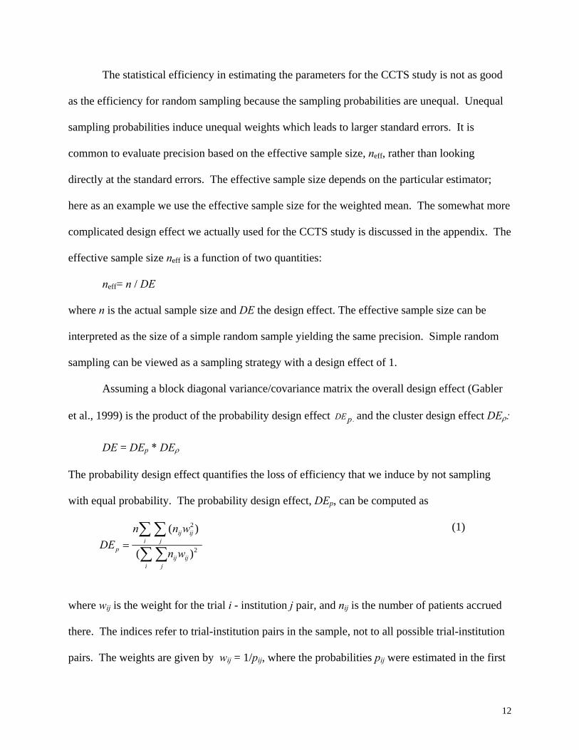
The statistical efficiency in estimating the parameters for the CCTS study is not as good

as the efficiency for random sampling because the sampling probabilities are unequal. Unequal

sampling probabilities induce unequal weights which leads to larger standard errors. It is

common to evaluate precision based on the effective sample size, neff, rather than looking

directly at the standard errors. The effective sample size depends on the particular estimator;

here as an example we use the effective sample size for the weighted mean. The somewhat more

complicated design effect we actually used for the CCTS study is discussed in the appendix. The

effective sample size neff is a function of two quantities:

neff= n / DE

where n is the actual sample size and DE the design effect. The effective sample size can be

interpreted as the size of a simple random sample yielding the same precision. Simple random

sampling can be viewed as a sampling strategy with a design effect of 1.

Assuming a block diagonal variance/covariance matrix the overall design effect (Gabler

et al., 1999) is the product of the probability design effect DE p and the cluster design effect DEρ:

DE = DEp * DEρ

The probability design effect quantifies the loss of efficiency that we induce by not sampling

with equal probability. The probability design effect, DEp, can be computed as

(1) 2

2

( )

( )

ij iji j

pij ij

i j

n n wDE

n w=

∑ ∑∑ ∑

where wij is the weight for the trial i - institution j pair, and nij is the number of patients accrued

there. The indices refer to trial-institution pairs in the sample, not to all possible trial-institution

pairs. The weights are given by wij = 1/pij, where the probabilities pij were estimated in the first

12

simulation as described earlier. Sampling with equal probability yields a probability design

effect of 1.

The cluster design effect quantifies the loss of efficiency by sampling clusters rather than

individual elements. Measurements of elements in clusters tend to be more correlated than those

of random elements. For computing the average cost the cluster design effect, DEρ, is

)1(1 −+= BDE ρρ (2)

where B is the average cluster size and ρ the intra-cluster correlation coefficient. As equation

(2) shows, the loss of efficiency – or design effect - increases with stronger intra-cluster

correlation and greater average cluster size.

When computing the difference in costs between cases and controls rather than the

average cost it is not obvious what the cluster design effect is. Controls are cancer patients,

comparable to cases, who received care at the participating institutions but did not enroll in any

clinical trial. We derive the design effect in Appendix A assuming that observations within

trial/institution pairs are correlated and the between pairs correlation is negligible. We believe

this is a reasonable assumption in the design stage for many problems. In the design stage, the

largest correlation is often used to approximate the complete correlation structure. In this case it

is wise to assume a somewhat larger value for the correlation. If the study designer has intuition

or data on several correlations they could easily be incorporated using a derivation analogous to

the derivation in Appendix A. In the CCTS example we have assumed that the dominant

correlation is the within trials correlation. If our candidate designs were found to select many

trial / institution pairs from single institutions we would need to reconsider the importance of the

within institution correlation.

13

We draw a large number of two-stage samples and compute the design effect and the

sample size for each sample. This yields an empirical joint distribution for the actual sample

size, the design effect, and the effective sample size. However, the distribution is generated by

drawing many samples from a particular study design. For any one study like the CCTS we

draw only one sample, and it is important to also investigate how bad a single unlucky draw may

be. Unlucky draws correspond to the upper tail of the distribution of the design effect. Hence a

good distribution has two features: the average (or median) design effect is small, and the

distribution of design effects does not have a large right tail. We therefore monitor both the

median and the 90th percentile of the distribution of the design effect. Generally, the design

effect tends to decrease the more homogeneous the selection probabilities, ijp , are. Excluding

trials and institutions with small accrual, i.e., raising the cutoffs, tends to accomplish that.

3.4. Choose the design that is the best compromise among the goals

As mentioned before, we consider the goals of high precision of estimates and good

coverage meeting the cost constraints. Usually all design goals cannot be optimized

simultaneously, therefore, the design of choice is a compromise. If the compromise could be

quantified in form of a loss or utility function, one could engage in formal optimization of the

loss function. In practice the researcher rarely has an explicit tradeoff between competing design

goals in mind. Also, routine optimization may overlook attractive alternatives. We prefer a

conscious compromise in which we are aware of the tradeoffs. What tradeoffs are acceptable

very much depends on the context of the problem at hand. Once a design has been chosen, a

single final sample is drawn.

The method described here has been implemented in Stata. The program can be obtained

by sending an e-mail to dana_goldman@rand.org.

14

4 Results

The goal of the Cost of Cancer Treatment Study (CCTS) is to estimate medical costs

incurred by patients who enroll in a clinical trial relative to patients who do not enroll in any

clinical trial. The target population for the CCTS study consists of all patients in phase III

clinical cancer trials that are conducted by cooperative oncology groups of the NCI. The data

were collected between October 1, 1998 and December 31, 1999.

The original power calculations were a typical lognormal health care costs analysis. We

assumed that health care costs are positively skewed and are normally distributed after a

logarithmic transformation. Similar data was analyzed and an unadjusted coefficient of variation

of 0.95 was observed. In similar settings we have typically achieved reductions in variance of

costs of 15-20% through multivariate analysis. We assumed the same coefficient of variation for

both trial participants and the non-trial participant control groups. With these assumptions 750

cases and 750 controls would have 80%-90% power to detect a cost difference of 10%.

The power calculations are only used to guide a first choice of the number of trials and

institutions needed. Guidance as to which values to choose for the trial and institution cutoffs

can be obtained from looking at histograms or simple frequency tables of institution and trial

sizes. Figure 2 shows how many patients were accrued at trials by size of the trials for the CCTS

study. Figure 3 shows the analogous histogram for institutions. A small number of simulations

with very few iterations can also help to quickly distinguish between realistic and unrealistic

parameter values.

*** Figures 2 and 3 here ***

15

Based on these histograms and on initial simulations, we consider trial cutoff values of

18, 24, and 30, and we consider institution cutoff values of 6, 9 and 12. There is no hard rule as

to how to choose these numbers. It is important, however, to examine a wide range of cutoffs.

For the trial and institution count values we consider three scenarios: sampling 35 trials/

55 institutions; 50 trials/ 40 institutions and 45 trials/ 50 institutions. For each scenario, we then

consider 3 different values for each design parameter: 18, 24, and 30, for trial cutoff; 6, 9, and 12

for institution cutoff; and 0.5, 0.75 and 1 for α. This yields 3*3*3*3=81 possible combinations

of design parameters. For each of the 81 runs, the simulations are as follows: For each

simulation, we run 7500 iterations to determine the sampling probabilities.

For each simulation, we select the 5 largest institutions purposively and the remaining

institutions as described earlier. We would likely reject any sample that does not include many

of the very large institutions. Rather than rejecting undesirable samples and making sampling

probabilities unnecessarily difficult to compute, we purposively select some institutions and let

the corresponding smaller weights reflect this inclusion. After selecting the trials we set the

inclusion probability of some institutions to one and simulate the inclusion probabilities of the

remaining institutions. Note that the largest institutions vary from sample to sample depending

on the trials selected.

Purposively including some institutions (i.e., sampling some institutions with probability

1) does not constitute “cheating.” On the contrary, it illustrates how easy it is to accommodate

study specific inclusion criteria by making minor modifications to the simulations. Not doing so

would mean modeling a slightly different sampling approach than is actually used. The effect of

incorporating this common practice in our model is a slightly larger design effect.

16

Each sample for the simulation in Step 2 can be drawn as follows: (a) A list of all trials is

constructed. Trials with too few patients according to the trial cutoff are eliminated from this

list. (This only need be done once for each design). (b) A sample of trials is drawn from this list.

(c) From the sampled trials a list of associated institutions is constructed. Institutions that do not

have enough patients based on the institution cutoff are eliminated from this list. (d) Institutions

are sampled from this list. The sample consists of all institutions/trial pairs for which both the

trial and the institution were sampled.

Having determined the sampling probabilities we were then able to estimate the design

effect. We ran 400 additional iterations and computed the design effect for each of the iterations

using equation (1). The calculation of the design effect requires the sampling probabilities pij,

which can only be computed after the last run of the first simulation.

In the Stata implementation of the program a simulation that draws 7500 samples to

compute the probabilities pij and 400 samples to compute the design effect based on the pij’s

takes about 1.6 hours on a laptop with a 1Ghz processor and 512K of RAM. Simulations can be

run in parallel. For example, with 4 workstations it is possible to run about 32-36 simulations

over night.

As a first step in selecting the design, we can now choose between the three trial and

institution count values scenarios. The curves that show the trade-off between coverage and

effective sample size are a useful graphical summary of the three scenarios. Figure 4 presents

the tradeoff curves for these three scenarios. For each scenario the 27 design combinations are

plotted. To make it easier to distinguish different sets of admissible points for each scenario we

connect the admissible points. Admissible points are points for which no other point exists that

has both better coverage and a greater effective sample size. The 45 trials/ 50 institutions curve

17

dominates the 35 trials/ 55 institutions curve (except in one small section), which in turn

dominates the 50 trials/ 40 institutions curve. One curve dominates another if the two curves do

not cross. This implies that for any point on the dominated curve there exists a point on the

dominating curve that is uniformly better.

We can see clearly as coverage increases effective sample size decreases. As coverage

increases the range of the selection probabilities increases, inducing a larger design effect, which

translates to a smaller effective sample size.

Our methodology was developed in response to the complexity of this study, but not in

time to be used in the design phase of this study. The scenario chosen in our study was 35 trials

and 55 institutions. Relative to this scenario we see that adding 10 additional trials and removing

5 institutions is beneficial. However, adding 15 additional trials and removing 15 institutions is

a bad idea. Adding 15 additional trials in our study meant sampling almost all (in some cases

all) trials eligible that had at least as many patients as specified in the trial cutoff value. This

suggests that the turning point at which adding trials at the expense of institutions becomes

disadvantageous is reached only after a large fraction of trials in the sample frame is already

sampled.

*** Figure 4 here ***

The run corresponding to our study is plotted with a diamond symbol in Figure 4. It has

an effective sample size of 793 and a sample frame coverage of 63.37%. It corresponds to an

institution cutoff of 9, a trial cutoff of 18, and an α of 1. This means that we are drawing trials

and institutions proportional to size.

Table 1 gives various statistics for all combinations of levels for the scenario with 35

trials and 55 institutions. Specifically, we report on the sample frame coverage, the median

18

accrual (i.e., median sample size), the median design effect, the median effective sample size,

and the 90th percentile of the design effect. We also report on the median probability and cluster

design effects separately. Most of the design effect stems from the unequal weights inducing the

probability design effect, relatively little from the clustering. The sample size in Table 1 refers

only to the number of cases. Because of the differencing between cases and controls, for the

CCTS we obtained an equal number of controls. Our study has the parameters Trial Cutoff = 18,

Institution Cutoff=9 and α=1. The correlation between the median design effect and the 90th

percentile for Table 1 is 42%. Because there is only moderate correlation the run with the best

median design effect may not have a favorable 90th percentile design effect.

*** Table 1 here ***

On closer examination, the runs in Figure 4 appear to be clustered in groups of three with each of

these groups having the same coverage. The clusters correspond to the three different levels of

α. This implies, while the choice of α clearly affects the effective sample size, α is less

important than the other factors we are investigating (trial cutoff, institution cutoff, number of

trials, number of institutions). Moreover, as can be seen from Table 1, all other factors being

constant, sampling proportional to size (α=1) is often inferior to α=0.5 and α=0.75.

4.1. Study sample

Finally, we generate one sample sampling proportionally to size and with cutoffs 18 and

9 for trials and institutions, respectively. The final sample yields a design effect of 1.28, below

the median as indicated in the first row of Table 1. After dropping institutions with an accrual of

less than 9 patients across the 35 sampled trials, there are about 110 institutions left, 55 of which

we sample. Each of the 55 institutions we sample participates in 3 to 14 of the sampled trials.

19

5 Discussion

We have presented a simulation-based approach for examining multiple sampling

goals for a multi-stage study design in which the levels are not strictly nested within one

another. In evaluating the sampling goals, we use simulations to estimate quantities such as

the sampling probabilities, which cannot easily be computed analytically due to the

complexity of the design. In the CCTS we have focused on sample frame coverage and the

effective sample size (which is equivalent to considering the standard error of the estimates)

and considered cost indirectly by evaluating the implications of trading additional trials for

less institutions.

The potential significance of our research is in its contribution to more economical

study design. The analysis needs to take into account the design structure. Mixed model

regression could be used, for example, specifying trial and institutions as random effects with

a suitable covariance matrix. Another option is generalized estimating equations (GEE),

which is asymptotically robust against misspecification of the covariance matrix. For the

CCTS this option is preferable given the large number of trials and institutions.

The design economies are twofold. First, it is possible to produce sampling plans that

may produce more of everything in some cases. The removal of the constraint that the

researcher must use one of a relatively small collection of standard approaches can yield

better designs for all of the objectives simultaneously in some cases. For example, we have

demonstrated that a tradeoff between the number of trials and institutions sampled can lead to

tradeoff curves that dominate one another. Second, these methods allow the design team to

consider more options more thoroughly. We believe that good tools that help in the design

process will prove to be very useful to the researcher.

20

Another useful feature of this approach is that it can be easily adapted to problems

that arise in the field. For example, samples must occasionally be reduced because of cost

overruns; an unexpectedly large number of trials or institutions may refuse to participate or

additional funds may make sample expansion possible. Dealing with all these problems

while still maintaining a probability sample is straightforward. The simulations are merely

expanded to include the additional actions being considered and new sampling probabilities,

design effects and coverages are calculated.

Our approach is less attractive when the stages of the multi-stage design are fully

nested within one another. In this case the sampling probabilities can be easily computed and

need not be simulated. Nonetheless, exploring the tradeoffs among the design goals remains

an attractive feature.

Appendix

In this appendix we derive the design effect for computing the difference between the

average cost for cases and the average cost for controls.

Denote the log costs of cases by , and the log cost of controls by . (The

logarithm of cost is used so that we can assume a normal distribution and a constant variance

in the power calculations below.) As before and

ijky ijkz

i j enumerate the trials and institutions

respectively. We assume that the design aims to obtain the same number of controls and

cases within each trial/institution pair. We assume the following model:

∑∑ −

=ij ijij

ij ijijijij

nw

zynwQ

)(

21

where are the sampling weights and are the number of cases in trial/institution pair ij .

If there is no difference in cost between cases and controls then . Further, we

assume

ijw ijn

0)( =QE

2)( σ=ijkyVar

⎩⎨⎧

=0

),(2

'''ρσ

kjiijk yyCov if otherwise

jjii ′=′= ;

(3)

where k enumerates the cases within trial/institution pairs. We use the same variance

/covariance model for the controls and cases. This is the same variance /covariance structure

used by Gable et al. (1999) in justifying Kish’s formula for design effects. In other words,

observations within trial/institution pairs are correlated, observations between trials or

between institutions are uncorrelated. Other correlations could be incorporated by modifying

(3). The correlation structure we specify reflects our belief that the within trial/institution

correlation is likely the largest correlation. Assuming σ2Y = σ2

Z and an equal number of

controls and cases in each cluster it follows that

Var ijijij nzy /)1(*2)( 2σρ−=− . (4)

Then the variance of the estimate of turns out to be Q

( )[ ]ρσ 21)(

2)( 22

2

−+ΣΣ

= bnwnw

QVar ijijijij

where

nwnw

bij

ij

Σ

Σ=

2

22

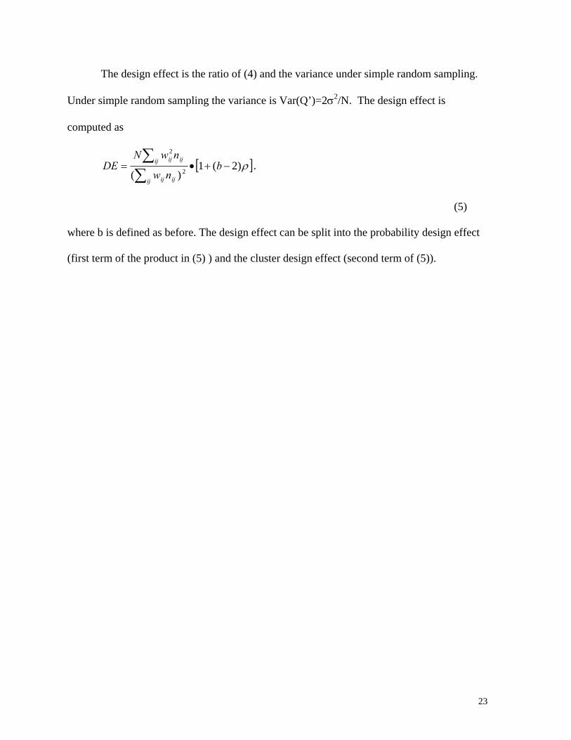
The design effect is the ratio of (4) and the variance under simple random sampling.

Under simple random sampling the variance is Var(Q’)=2σ2/N. The design effect is

computed as

[ ]ρ)2(1)( 2

2

−+•=∑∑

bnw

nwNDE

ij ijij

ijij ij.

(5)

where b is defined as before. The design effect can be split into the probability design effect

(first term of the product in (5) ) and the cluster design effect (second term of (5)).

23

References

(1) Anderson, R., Kasper, J., Frankel, M. and Associates, Total survey error, Jossey-Bass Publishers, San Francisco, 1979. (2) Cochran, W.G., Sampling techniques, John Wiley & Sons, New York, 3rd ed, 1997. (3) Frankel, M.R., Shapiro, M.F., Duan, N., Morton, S.C., Berry, S.H., Brown, J.A., Burnam, M.A., Cohn, S.E., Goldman, D.P., McCaffrey, D.F., Smith, S.M., St Clair, P.A., Tebow, J.F. and Bozzette, S.A.,“National probability samples in studies of low-prevalence diseases. Part II: designing and implementing the HIV cost and services utilization study sample,” Health Services Research, 34, 5, 969-992, 1999. (4) Gabler, S., Haeder, S. and Lahiri, P., “A model based Justification of Kish’s formula for design effects for weighting and clustering,” Survey Methodology, 25, 1, 105-106, 1999. (5) Goldman D., Adams, J.L., Berry, S.H., Escarce, J.J., Kilgore, M., Lewis, J., Rosen, M.R., Schoenbaum, M.L., Schonlau, M., Wagle, N. and Weidmer, B.A., “Measuring the incremental costs of clinical cancer research: the cost of cancer treatment study,” RAND, Santa Monica, CA, report MR-1169-NSF, 2000. (6) Kish, L., Survey sampling, John Wiley & Sons, New York, 1965. (7) Linacre, S., Trewin, D., “Total survey design – application to a collection of the construction industry,” Journal of Official Statistic, 9, 3, 611-621, 1993. (8) Mansour, E.G., “Barriers to clinical trials. Part III: knowledge and attitudes of health care providers,” Cancer, 74, (suppl 9), 2672-2675, 1994. (9) Morrow, G.R., Hickok, J.T. and Burish, T.G., “Behavioral aspects of clinical trials. An integrated framework from behavior theory,” Cancer, 74, (suppl 9), 2676-2682, 1994. (10) Shapiro, M.F., Berk, M.L., Berry, S.H., Emmons, C.A., Athey, L.A., Hsia, D.C., Leibowitz, A.A., Maida, C.A., Marcus, M., Perlman, J.F., Schur, C.L., Schuster, M.A., Senterfitt, J.W. and Bozzette, S.A., “National probability samples in studies of low-prevalence diseases. Part I: perspectives and lessons from the HIV cost and services utilizations study,” Health Services Research, 34, 5, 951-948, 1999. (11) Wagner, J.L., Alberts, S.R., Sloan, J.A., Cha, S., Killian, J., O’Connell, M.J., Van Grevenhof, P., Lindman, J. and Chute, C.G., “Incremental costs of enrolling cancer patients in clinical trials: a population-based study,” Journal of the National Cancer Institute, 91, 10, 847-853, 1999.

24

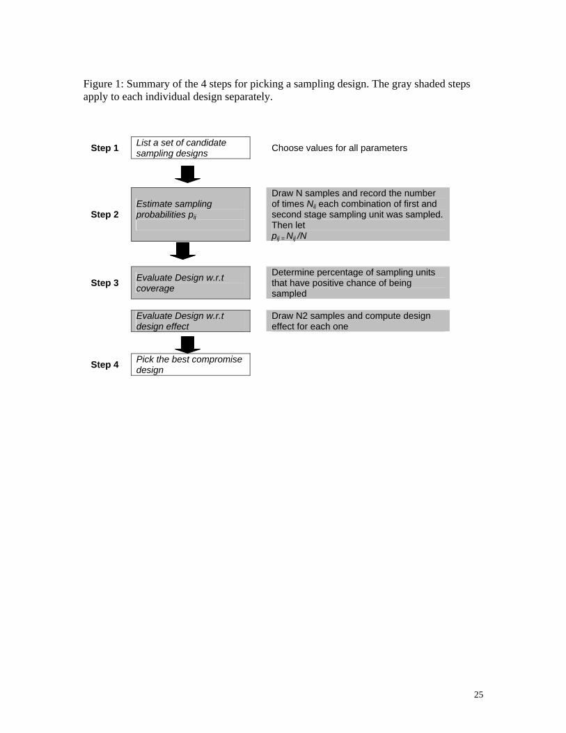
Figure 1: Summary of the 4 steps for picking a sampling design. The gray shaded steps apply to each individual design separately.

Step 1 List a set of candidate sampling designs

Choose values for all parameters

Step 2 Estimate sampling probabilities pij

Draw N samples and record the number of times Nij each combination of first and second stage sampling unit was sampled. Then let pij = Nij /N

Step 3 Evaluate Design w.r.t coverage

Determine percentage of sampling units that have positive chance of being sampled

Evaluate Design w.r.t design effect

Draw N2 samples and compute design effect for each one

Step 4 Pick the best compromise design

25

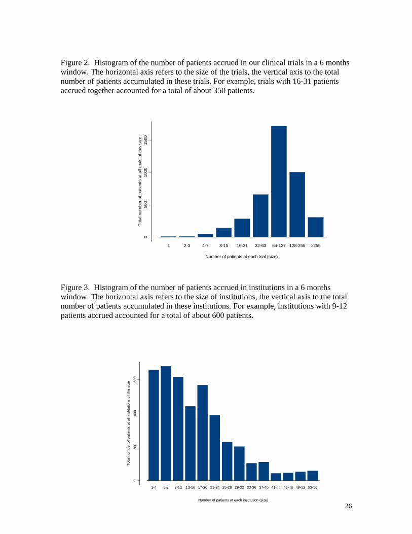
Figure 2. Histogram of the number of patients accrued in our clinical trials in a 6 months window. The horizontal axis refers to the size of the trials, the vertical axis to the total number of patients accumulated in these trials. For example, trials with 16-31 patients accrued together accounted for a total of about 350 patients.

050

010

0015

00

1 2-3 4-7 8-15 16-31 32-63 64-127 128-255 >255

Number of patients at each trial (size)

Tota

l num

ber o

f pat

ient

s at

all

trial

s of

this

siz

e

Figure 3. Histogram of the number of patients accrued in institutions in a 6 months window. The horizontal axis refers to the size of institutions, the vertical axis to the total number of patients accumulated in these institutions. For example, institutions with 9-12 patients accrued accounted for a total of about 600 patients.

020

040

060

0

1-4 5-8 9-12 13-16 17-20 21-24 25-28 29-32 33-36 37-40 41-44 45-48 49-52 53-56

Number of patients at each institution (size)

Tota

l num

ber o

f pat

ient

s at

all

inst

itutio

ns o

f thi

s si

ze

26

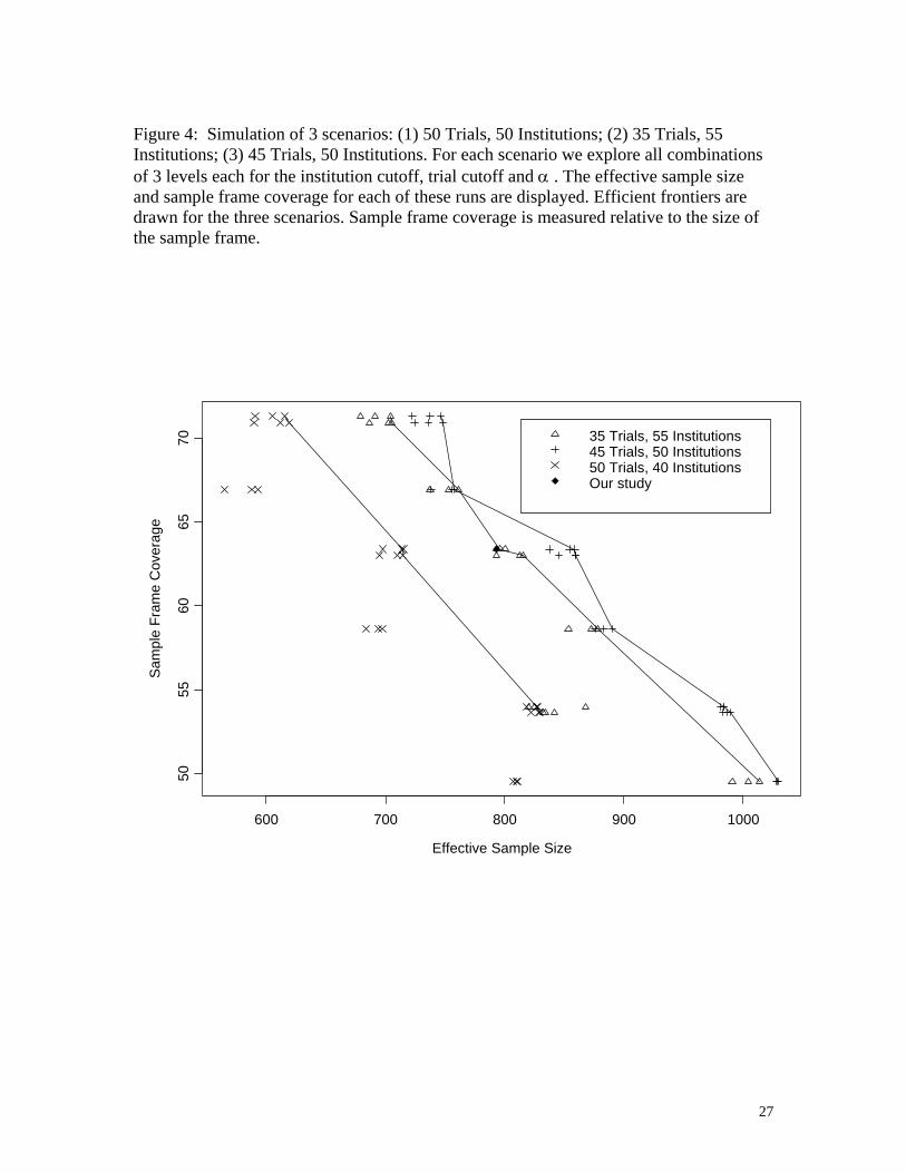
Figure 4: Simulation of 3 scenarios: (1) 50 Trials, 50 Institutions; (2) 35 Trials, 55 Institutions; (3) 45 Trials, 50 Institutions. For each scenario we explore all combinations of 3 levels each for the institution cutoff, trial cutoff and α . The effective sample size and sample frame coverage for each of these runs are displayed. Efficient frontiers are drawn for the three scenarios. Sample frame coverage is measured relative to the size of the sample frame.

Effective Sample Size

Sam

ple

Fram

e C

over

age

600 700 800 900 1000

5055

6065

70 35 Trials, 55 Institutions45 Trials, 50 Institutions50 Trials, 40 InstitutionsOur study

27

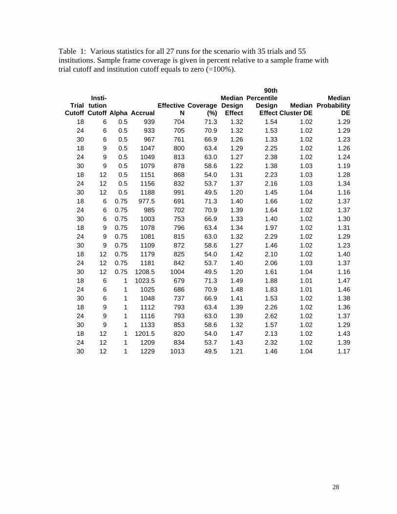
Table 1: Various statistics for all 27 runs for the scenario with 35 trials and 55 institutions. Sample frame coverage is given in percent relative to a sample frame with trial cutoff and institution cutoff equals to zero (=100%).

Trial Cutoff

Insti- tution Cutoff Alpha Accrual

Effective N

Coverage (%)

Median Design

Effect

90th Percentile

Design Effect

Median Cluster DE

Median Probability

DE18 6 0.5 939 704 71.3 1.32 1.54 1.02 1.2924 6 0.5 933 705 70.9 1.32 1.53 1.02 1.2930 6 0.5 967 761 66.9 1.26 1.33 1.02 1.2318 9 0.5 1047 800 63.4 1.29 2.25 1.02 1.2624 9 0.5 1049 813 63.0 1.27 2.38 1.02 1.2430 9 0.5 1079 878 58.6 1.22 1.38 1.03 1.1918 12 0.5 1151 868 54.0 1.31 2.23 1.03 1.2824 12 0.5 1156 832 53.7 1.37 2.16 1.03 1.3430 12 0.5 1188 991 49.5 1.20 1.45 1.04 1.1618 6 0.75 977.5 691 71.3 1.40 1.66 1.02 1.3724 6 0.75 985 702 70.9 1.39 1.64 1.02 1.3730 6 0.75 1003 753 66.9 1.33 1.40 1.02 1.3018 9 0.75 1078 796 63.4 1.34 1.97 1.02 1.3124 9 0.75 1081 815 63.0 1.32 2.29 1.02 1.2930 9 0.75 1109 872 58.6 1.27 1.46 1.02 1.2318 12 0.75 1179 825 54.0 1.42 2.10 1.02 1.4024 12 0.75 1181 842 53.7 1.40 2.06 1.03 1.3730 12 0.75 1208.5 1004 49.5 1.20 1.61 1.04 1.1618 6 1 1023.5 679 71.3 1.49 1.88 1.01 1.4724 6 1 1025 686 70.9 1.48 1.83 1.01 1.4630 6 1 1048 737 66.9 1.41 1.53 1.02 1.3818 9 1 1112 793 63.4 1.39 2.26 1.02 1.3624 9 1 1116 793 63.0 1.39 2.62 1.02 1.3730 9 1 1133 853 58.6 1.32 1.57 1.02 1.2918 12 1 1201.5 820 54.0 1.47 2.13 1.02 1.4324 12 1 1209 834 53.7 1.43 2.32 1.02 1.3930 12 1 1229 1013 49.5 1.21 1.46 1.04 1.17

28

Affiliation of Authors

John L. Adams Ph.D., RAND, john_adams@rand.org

Matthias Schonlau Ph.D., RAND, matthias_schonlau@rand.org

José J. Escarce M.D., RAND, jose_escarce@rand.org

Meredith Kilgore M.S.P.H., University of Alabama, mkilgore@ms.soph.uab.edu

Michael Schoenbaum Ph.D., RAND, michael_schoenbaum@rand.org

Dana P. Goldman Ph.D., RAND, dana_goldman@rand.org

Corresponding Author: Matthias Schonlau

Office: RAND, Statistics Group, P.O. Box 2138, Santa Monica, CA, 90407-2138

Phone: 310-393-0411 x7682, email: matthias_schonlau@rand.org

Acknowledgement: The National Cancer Institute is providing principal funding for the Cost of Cancer Treatment Study. Additional funding comes from the Office of the Director, National Institutes of Health and by the National Science Foundation as part of its support for the White House's Office of Science and Technology Policy. The authors wish to thank Sandra Berry, Ronald Fricker, Richard Kaplan, Daniel McCaffrey, Michael Montello, Sally Morton, Mary McCabe, Arnold Potosky, and Jane Weeks for their assistance in this research.

29