Sampling, Reconstruction, and Antialiasingwolberg/pub/crc04.pdf · Sampling, Reconstruction, and Antialiasing 39-3 FIGURE 39.2 Spectrum G(f). 39.2.1 Sampling Consider a 1-D signal

39Sampling,

Reconstruction, andAntialiasing

George WolbergCity College of New York

39.1 Introduction . . . . . . . . . . . . . . . . . . . . . . . . . . . . . . . . . . . . . . . .39-139.2 Sampling Theory. . . . . . . . . . . . . . . . . . . . . . . . . . . . . . . . . . . .39-2

Sampling

39.3 Reconstruction . . . . . . . . . . . . . . . . . . . . . . . . . . . . . . . . . . . . .39-4Reconstruction Conditions • Ideal Low-Pass Filter • SincFunction • Nonideal Reconstruction

39.4 Reconstruction Kernels . . . . . . . . . . . . . . . . . . . . . . . . . . . . . .39-8Box Filter • Triangle Filter • Cubic Convolution• Windowed Sinc Function • Hann and Hamming Windows• Blackman Window • Kaiser Window • Lanczos Window

39.5 Aliasing . . . . . . . . . . . . . . . . . . . . . . . . . . . . . . . . . . . . . . . . . . . . .39-1339.6 Antialiasing . . . . . . . . . . . . . . . . . . . . . . . . . . . . . . . . . . . . . . . . .39-14

Point Sampling • Area Sampling • Supersampling• Adaptive Supersampling

39.7 Prefiltering. . . . . . . . . . . . . . . . . . . . . . . . . . . . . . . . . . . . . . . . . .39-18Pyramids • Summed-Area Tables

39.8 Example: Image Scaling . . . . . . . . . . . . . . . . . . . . . . . . . . . . .39-2139.9 Research Issues and Summary . . . . . . . . . . . . . . . . . . . . . . .39-25

39.1 Introduction

This chapter reviews the principal ideas of sampling theory, reconstruction, and antialiasing. Samplingtheory is central to the study of sampled-data systems, e.g., digital image transformations. It lays a firmmathematical foundation for the analysis of sampled signals, offering invaluable insight into the problemsand solutions of sampling. It does so by providing an elegant mathematical formulation describing therelationship between a continuous signal and its samples. We use it to resolve the problems of imagereconstruction and aliasing. Reconstruction is an interpolation procedure applied to the sampled data. Itpermits us to evaluate the discrete signal at any desired position, not just the integer lattice upon which thesampled signal is given. This is useful when implementing geometric transformations, or warps, on theimage. Aliasing refers to the presence of unreproducibly high frequencies in the image and the resultingartifacts that arise upon undersampling.

Together with defining theoretical limits on the continuous reconstruction of discrete input, samplingtheory yields the guidelines for numerically measuring the quality of various proposed filtering techniques.

1-58488-360-X/$0.00+$1.50© 2004 by CRC Press, LLC 39-1

39-2 Computer Science Handbook

FIGURE 39.1 Oblique checkerboard: (a) unfiltered, (b) filtered.

This proves most useful in formally describing reconstruction, aliasing, and the filtering necessary tocombat the artifacts that may appear at the output.

In order to better motivate the importance of sampling theory and filtering, we demonstrate its rolewith the following examples. A checkerboard texture is shown projected onto an oblique planar surface inFigure 39.1. The image exhibits two forms of artifacts: jagged edges and moire patterns. Jagged edges areprominent toward the bottom of the image, where the input checkerboard undergoes magnification. Itreflects poor reconstruction of the underlying signal. The moire patterns, on the other hand, are noticeableat the top, where minification (compression) forces many input pixels to occupy fewer output pixels. Thisartifact is due to aliasing, a symptom of undersampling.

Figure 39.1(a) was generated by projecting the center of each output pixel into the checkerboard andsampling (reading) the value of the nearest input pixel. This point sampling method performs poorly, asis evident by the objectionable results of Figure 39.1(a). This conclusion is reached by sampling theoryas well. Its role here is to precisely quantify this phenomenon and to prescribe a solution. Figure 39.1(b)shows the same mapping with improved results. This time the necessary steps were taken to precludeartifacts. In particular, a superior reconstruction algorithm was used for interpolation to suppress thejagged edges, and antialiasing filtering was carried out to combat the symptoms of undersampling thatgave rise to the moire patterns.

39.2 Sampling Theory

Both reconstruction and antialiasing share the twofold problem addressed by sampling theory:

1. Given a continuous input signal g (x) and its sampled counterpart gs (x), are the samples of gs (x)sufficient to exactly describe g (x)?

2. If so, how can g (x) be reconstructed from gs (x)?

The solution lies in the frequency domain, whereby spectral analysis is used to examine the spectrum ofthe sampled data.

The conclusions derived from examining the reconstruction problem will prove to be directly usefulfor resampling and indicative of the filtering necessary for antialiasing. Sampling theory thereby providesan elegant mathematical framework in which to assess the quality of reconstruction, establish theoreticallimits, and predict when it is not possible.

Sampling, Reconstruction, and Antialiasing 39-3

FIGURE 39.2 Spectrum G( f ).

39.2.1 Sampling

Consider a 1-D signal g (x) and its spectrum G( f ), as determined by the Fourier transform:

G( f ) =∫ ∞

−∞g (x)e−i2� f x dx (39.1)

Note that x represents spatial position and f denotes spatial frequency.The magnitude spectrum of a signal is shown in Figure 39.2. It shows the frequency content of the

signal, with a high concentration of energy in the low-frequency range, tapering off toward the higherfrequencies. Since there are no frequency components beyond fmax, the signal is said to be bandlimitedto frequency fmax.

The continuous output g (x) is then digitized by an ideal impulse sampler, the comb function, to getthe sampled signal gs (x). The ideal 1-D sampler is given as

s (x) =∞∑

n=−∞�(x − nTs ) (39.2)

where � is the familiar impulse function and Ts is the sampling period. The running index n is used with� to define the impulse train of the comb function. We now have

gs (x) = g (x)s (x) (39.3)

Taking the Fourier transform of gs (x) yields

G s ( f ) = G( f ) ∗ S( f ) (39.4)

= G( f ) ∗[

n=∞∑n=−∞

fs �( f − n fs )

](39.5)

= fs

n=∞∑n=−∞

G( f − n fs ) (39.6)

where fs is the sampling frequency and ∗ denotes convolution. The above equations make use of thefollowing well-known properties of Fourier transforms:

1. Multiplication in the spatial domain corresponds to convolution in the frequency domain. There-fore, Equation 39.3 gives rise to a convolution in Equation 39.4.

2. The Fourier transform of an impulse train is itself an impulse train, giving us Equation 39.5.3. The spectrum of a signal sampled with frequency fs (Ts = 1/ fs ) yields the original spectrum

replicated in the frequency domain with period fs Equation 39.6.


FIGURE 39.3 Spectrum G s ( f ).

This last property has important consequences. It yields a spectrum G s ( f ), which, in response to asampling period Ts = 1/ fs , is periodic in frequency with period fs . This is depicted in Figure 39.3. Notice,then, that a small sampling period is equivalent to a high sampling frequency, yielding spectra replicated farapart from each other. In the limiting case when the sampling period approaches zero (Ts → 0, fs → ∞),only a single spectrum appears — a result consistent with the continuous case.

39.3 Reconstruction

The above result reveals that the sampling operation has left the original input spectrum intact, merelyreplicating it periodically in the frequency domain with a spacing of fs . This allows us to rewrite G s ( f ) as asum of two terms, the low-frequency (baseband) and high-frequency components. The baseband spectrumis exactly G( f ), and the high-frequency components, G high( f ), consist of the remaining replicated versionsof G( f ) that constitute harmonic versions of the sampled image:

G s ( f ) = G( f ) + G high( f ) (39.7)

Exact signal reconstruction from sampled data requires us to discard the replicated spectra G high( f ),leaving only G( f ), the spectrum of the signal we seek to recover. This is a crucial observation in the studyof sampled-data systems.

39.3.1 Reconstruction Conditions

The only provision for exact reconstruction is that G( f ) be undistorted due to overlap with G high( f ).Two conditions must hold for this to be true:

1. The signal must be bandlimited. This avoids spectra with infinite extent that are impossible toreplicate without overlap.

2. The sampling frequency fs must be greater than twice the maximum frequency fmax present in thesignal. This minimum sampling frequency, known as the Nyquist rate, is the minimum distancebetween the spectra copies, each with bandwidth fmax.

The first condition merely ensures that a sufficiently large sampling frequency exists that can be used toseparate replicated spectra from each other. Since all imaging systems impose a bandlimiting filter in theform of a point spread function, this condition is always satisfied for images captured through an opticalsystem. Note that this does not apply to synthetic images, e.g., computer-generated imagery.

The second condition proves to be the most revealing statement about reconstruction. It answers theproblem regarding the sufficiency of the data samples to exactly reconstruct the continuous input signal.It states that exact reconstruction is possible only when fs > fNyquist, where fNyquist = 2 fmax. Collectively,these two conclusions about reconstruction form the central message of sampling theory, as pioneered byClaude Shannon in his landmark papers on the subject [Shannon 1948, 1949].


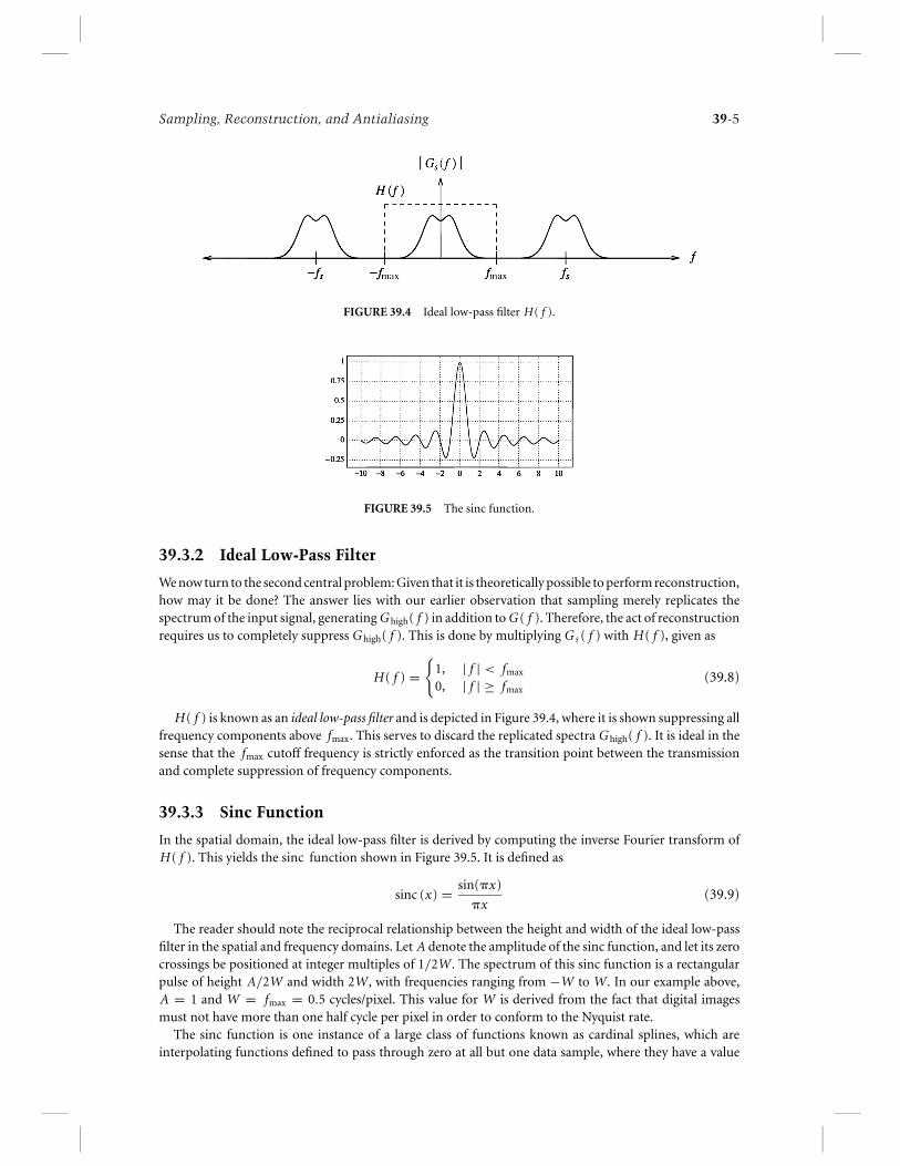
FIGURE 39.4 Ideal low-pass filter H( f ).

FIGURE 39.5 The sinc function.

39.3.2 Ideal Low-Pass Filter

We now turn to the second central problem: Given that it is theoretically possible to perform reconstruction,how may it be done? The answer lies with our earlier observation that sampling merely replicates thespectrum of the input signal, generating G high( f ) in addition to G( f ). Therefore, the act of reconstructionrequires us to completely suppress G high( f ). This is done by multiplying G s ( f ) with H( f ), given as

H( f ) ={

1, | f | < fmax

0, | f | ≥ fmax(39.8)

H( f ) is known as an ideal low-pass filter and is depicted in Figure 39.4, where it is shown suppressing allfrequency components above fmax. This serves to discard the replicated spectra G high( f ). It is ideal in thesense that the fmax cutoff frequency is strictly enforced as the transition point between the transmissionand complete suppression of frequency components.

39.3.3 Sinc Function

In the spatial domain, the ideal low-pass filter is derived by computing the inverse Fourier transform ofH( f ). This yields the sinc function shown in Figure 39.5. It is defined as

sinc (x) = sin(�x)

�x(39.9)

The reader should note the reciprocal relationship between the height and width of the ideal low-passfilter in the spatial and frequency domains. Let A denote the amplitude of the sinc function, and let its zerocrossings be positioned at integer multiples of 1/2W. The spectrum of this sinc function is a rectangularpulse of height A/2W and width 2W, with frequencies ranging from −W to W. In our example above,A = 1 and W = fmax = 0.5 cycles/pixel. This value for W is derived from the fact that digital imagesmust not have more than one half cycle per pixel in order to conform to the Nyquist rate.

The sinc function is one instance of a large class of functions known as cardinal splines, which areinterpolating functions defined to pass through zero at all but one data sample, where they have a value


FIGURE 39.6 Truncation in one domain causes ringing in the other domain.

of one. This allows them to compute a continuous function that passes through the uniformly spaced datasamples.

Since multiplication in the frequency domain is identical to convolution in the spatial domain, sinc (x)represents the convolution kernel used to evaluate any point x on the continuous input curve g given onlythe sampled data gs :

g (x) = sinc (x) ∗ gs (x) =∫ ∞

−∞sinc (�) gs (x − �) d� (39.10)

Equation 39.10 highlights an important impediment to the practical use of the ideal low-pass filter.The filter requires an infinite number of neighboring samples (i.e., an infinite filter support) in orderto precisely compute the output points. This is, of course, impossible owing to the finite number ofdata samples available. However, truncating the sinc function allows for approximate solutions to becomputed at the expense of undesirable “ringing,” i.e., ripple effects. These artifacts, known as the Gibbsphenomenon, are the overshoots and undershoots caused by reconstructing a signal with truncatedfrequency terms. The two rows in Figure 39.6 show that truncation in one domain leads to ringing in theother domain. This indicates that a truncated sinc function is actually a poor reconstruction filter becauseits spectrum has infinite extent and thereby fails to bandlimit the input.

In response to these difficulties, a number of approximating algorithms have been derived, offering atradeoff between precision and computational expense. These methods permit local solutions that requirethe convolution kernel to extend only over a small neighborhood. The drawback, however, is that thefrequency response of the filter has some undesirable properties. In particular, frequencies below fmax aretampered, and high frequencies beyond fmax are not fully suppressed. Thus, nonideal reconstruction doesnot permit us to exactly recover the continuous underlying signal without artifacts.

39.3.4 Nonideal Reconstruction

The process of nonideal reconstruction is depicted in Figure 39.7, which indicates that the input signalsatisfies the two conditions necessary for exact reconstruction. First, the signal is bandlimited, since thereplicated copies in the spectrum are each finite in extent. Second, the sampling frequency exceeds theNyquist rate, since the copies do not overlap. However, this is where our ideal scenario ends. Instead of


FIGURE 39.7 Nonideal reconstruction.

using an ideal low-pass filter to retain only the baseband spectrum components, a nonideal reconstructionfilter is shown in the figure.

The filter response Hr ( f ) deviates from the ideal response H( f ) shown in Figure 39.4. In particular,Hr ( f ) does not discard all frequencies beyond fmax. Furthermore, that same filter is shown to attenuatesome frequencies that should have remained intact. This brings us to the problem of assessing the qualityof a filter.

The accuracy of a reconstruction filter can be evaluated by analyzing its frequency-domain character-istics. Of particular importance is the filter response in the passband and stopband. In this problem, thepassband consists of all frequencies below fmax. The stopband contains all higher frequencies arising fromthe sampling process.

An ideal reconstruction filter, as described earlier, will completely suppress the stopband while leavingthe passband intact. Recall that the stopband contains the offending high frequencies that, if allowed toremain, would prevent us from performing exact reconstruction. As a result, the sinc filter was devisedto meet these goals and serve as the ideal reconstruction filter. Its kernel in the frequency domain appliesunity gain to transmit the passband and zero gain to suppress the stopband.

The breakdown of the frequency domain into passband and stopband isolates two problems that can arisedue to nonideal reconstruction filters. The first problem deals with the effects of imperfect filtering on thepassband. Failure to impose unity gain on all frequencies in the passband will result in some combinationof image smoothing and image sharpening. Smoothing, or blurring, will result when the frequency gainsnear the cutoff frequency start falling off. Image sharpening results when the high-frequency gains areallowed to exceed unity. This follows from the direct correspondence of visual detail to spatial frequency.Furthermore, amplifying the high passband frequencies yields a sharper transition between the passbandand stopband, a property shared by the sinc function.

The second problem addresses nonideal filtering on the stopband. If the stopband is allowed to persist,high frequencies will exist that will contribute to aliasing (described later). Failure to fully suppress thestopband is a condition known as frequency leakage. This allows the offending frequencies to fold overinto the passband range. These distortions tend to be more serious, since they are visually perceived morereadily.

In the spatial domain, nonideal reconstruction is achieved by centering a finite-width kernel at theposition in the data at which the underlying function is to be evaluated, i.e., reconstructed. This is aninterpolation problem which, for equally spaced data, can be expressed as

f (x) =K −1∑k=0

f (xk)h(x − xk) (39.11)

where h is the reconstruction kernel that weighs K data samples at xk . Equation 39.11 formulates interpo-lation as a convolution operation. In practice, h is nearly always a symmetric kernel, i.e., h(−x) = h(x).We shall assume this to be true in the discussion that follows.

The computation of one interpolated point is illustrated in Figure 39.8. The kernel is centered at x , thelocation of the point to be interpolated. The value of that point is equal to the sum of the values of the


FIGURE 39.8 Interpolation of a single point.

FIGURE 39.9 Box filter: (a) kernel, (b) Fourier transform.

discrete input scaled by the corresponding values of the reconstruction kernel. This follows directly fromthe definition of convolution.

39.4 Reconstruction Kernels

The numerical accuracy and computational cost of reconstruction are directly tied to the convolution kernelused for low-pass filtering. As a result, filter kernels are the target of design and analysis in the creation andevaluation of reconstruction algorithms. They are subject to conditions influencing the tradeoff betweenaccuracy and efficiency. This section reviews several common nonideal reconstruction filter kernels in theorder of their complexity: box filter, triangle filter, cubic convolution, and windowed sinc functions.

39.4.1 Box Filter

The box filter kernel is defined as

h(x) ={

1, −0.5 < x ≤ 0.5

0, otherwise(39.12)

Various other names are used to denote this simple kernel, including the sample-and-hold function andFourier window. The kernel and its Fourier transform are shown in Figure 39.9.

Convolution in the spatial domain with the rectangle function h is equivalent in the frequency domainto multiplication with a sinc function. Due to the prominent side lobes and infinite extent, a sinc function


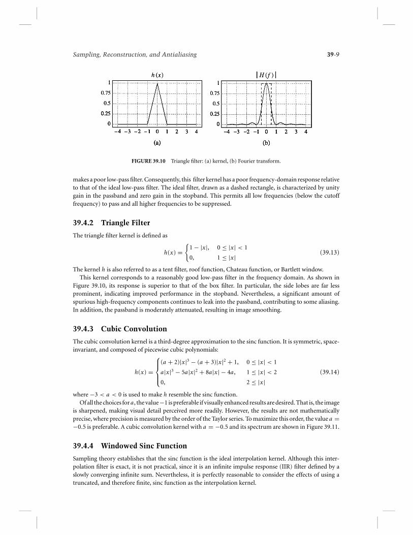
FIGURE 39.10 Triangle filter: (a) kernel, (b) Fourier transform.

makes a poor low-pass filter. Consequently, this filter kernel has a poor frequency-domain response relativeto that of the ideal low-pass filter. The ideal filter, drawn as a dashed rectangle, is characterized by unitygain in the passband and zero gain in the stopband. This permits all low frequencies (below the cutofffrequency) to pass and all higher frequencies to be suppressed.

39.4.2 Triangle Filter

The triangle filter kernel is defined as

h(x) ={

1 − |x|, 0 ≤ |x| < 1

0, 1 ≤ |x| (39.13)

The kernel h is also referred to as a tent filter, roof function, Chateau function, or Bartlett window.This kernel corresponds to a reasonably good low-pass filter in the frequency domain. As shown in

Figure 39.10, its response is superior to that of the box filter. In particular, the side lobes are far lessprominent, indicating improved performance in the stopband. Nevertheless, a significant amount ofspurious high-frequency components continues to leak into the passband, contributing to some aliasing.In addition, the passband is moderately attenuated, resulting in image smoothing.

39.4.3 Cubic Convolution

The cubic convolution kernel is a third-degree approximation to the sinc function. It is symmetric, space-invariant, and composed of piecewise cubic polynomials:

h(x) =

(a + 2)|x|3 − (a + 3)|x|2 + 1, 0 ≤ |x| < 1

a|x|3 − 5a|x|2 + 8a|x| − 4a , 1 ≤ |x| < 2

0, 2 ≤ |x|(39.14)

where −3 < a < 0 is used to make h resemble the sinc function.Of all the choices for a , the value−1 is preferable if visually enhanced results are desired. That is, the image

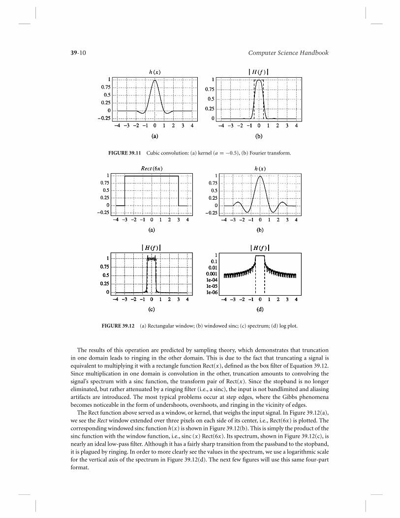
is sharpened, making visual detail perceived more readily. However, the results are not mathematicallyprecise, where precision is measured by the order of the Taylor series. To maximize this order, the value a =−0.5 is preferable. A cubic convolution kernel with a = −0.5 and its spectrum are shown in Figure 39.11.

39.4.4 Windowed Sinc Function

Sampling theory establishes that the sinc function is the ideal interpolation kernel. Although this inter-polation filter is exact, it is not practical, since it is an infinite impulse response (IIR) filter defined by aslowly converging infinite sum. Nevertheless, it is perfectly reasonable to consider the effects of using atruncated, and therefore finite, sinc function as the interpolation kernel.


FIGURE 39.11 Cubic convolution: (a) kernel (a = −0.5), (b) Fourier transform.

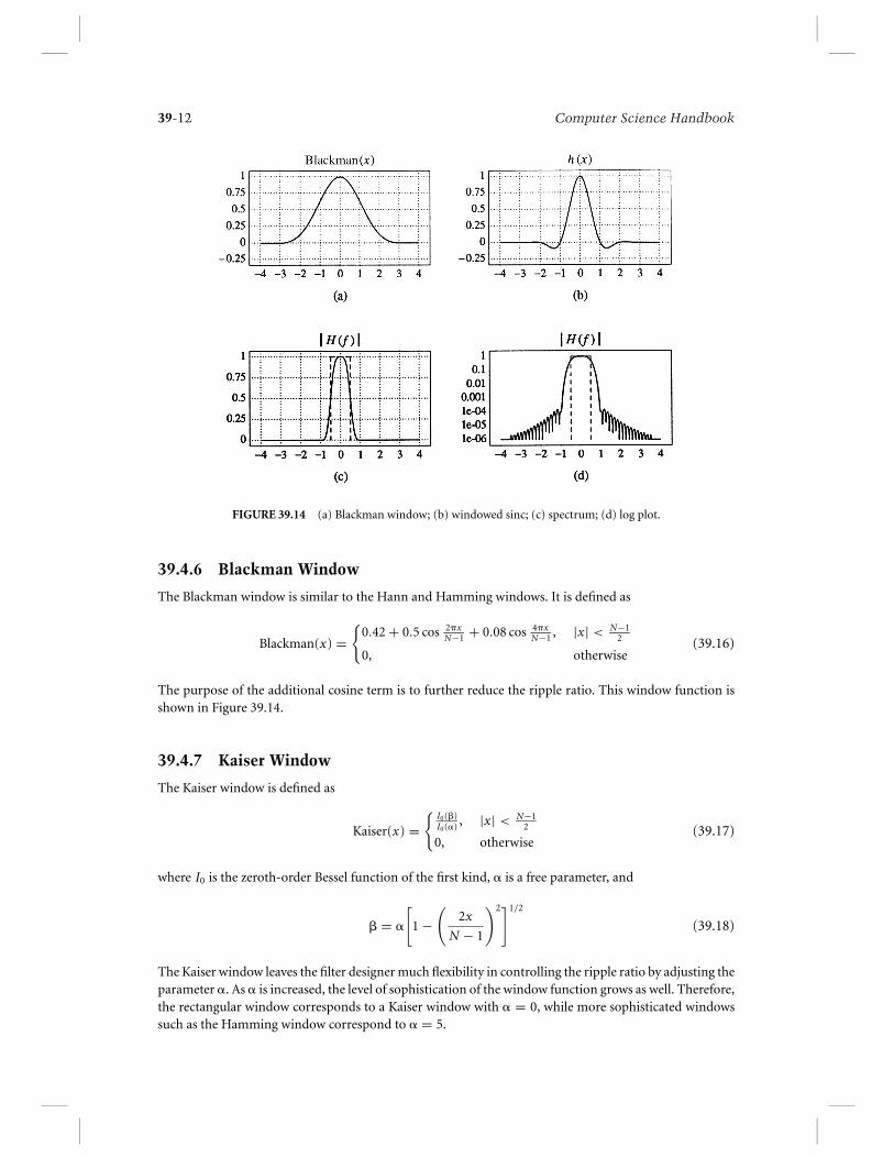
FIGURE 39.12 (a) Rectangular window; (b) windowed sinc; (c) spectrum; (d) log plot.

The results of this operation are predicted by sampling theory, which demonstrates that truncationin one domain leads to ringing in the other domain. This is due to the fact that truncating a signal isequivalent to multiplying it with a rectangle function Rect(x), defined as the box filter of Equation 39.12.Since multiplication in one domain is convolution in the other, truncation amounts to convolving thesignal’s spectrum with a sinc function, the transform pair of Rect(x). Since the stopband is no longereliminated, but rather attenuated by a ringing filter (i.e., a sinc), the input is not bandlimited and aliasingartifacts are introduced. The most typical problems occur at step edges, where the Gibbs phenomenabecomes noticeable in the form of undershoots, overshoots, and ringing in the vicinity of edges.

The Rect function above served as a window, or kernel, that weighs the input signal. In Figure 39.12(a),we see the Rect window extended over three pixels on each side of its center, i.e., Rect(6x) is plotted. Thecorresponding windowed sinc function h(x) is shown in Figure 39.12(b). This is simply the product of thesinc function with the window function, i.e., sinc (x) Rect(6x). Its spectrum, shown in Figure 39.12(c), isnearly an ideal low-pass filter. Although it has a fairly sharp transition from the passband to the stopband,it is plagued by ringing. In order to more clearly see the values in the spectrum, we use a logarithmic scalefor the vertical axis of the spectrum in Figure 39.12(d). The next few figures will use this same four-partformat.


Ringing can be mitigated by using a different windowing function exhibiting smoother falloff thanthe rectangle. The resulting windowed sinc function can yield better results. However, since slow falloffrequires larger windows, the computation remains costly.

Aside from the rectangular window mentioned above, the most frequently used window functions areHann, Hamming, Blackman, and Kaiser. These filters identify a quantity known as the ripple ratio, definedas the ratio of the maximum side-lobe amplitude to the main-lobe amplitude. Good filters will have smallripple ratios to achieve effective attenuation in the stopband. A tradeoff exists, however, between rippleratio and main-lobe width. Therefore, as the ripple ratio is decreased, the main-lobe width is increased.This is consistent with the reciprocal relationship between the spatial and frequency domains, i.e., narrowbandwidths correspond to wide spatial functions.

In general, though, each of these smooth window functions is defined over a small finite extent. Thisis tantamount to multiplying the smooth window with a rectangle function. While this is better than theRect function alone, there will inevitably be some form of aliasing. Nevertheless, the window functionsdescribed below offer a good compromise between ringing and blurring.

39.4.5 Hann and Hamming Windows

The Hann and Hamming windows are defined as

Hann/Hamming(x) ={

� + (1 − �) cos 2�xN−1 , |x| < N−1

2

0, otherwise(39.15)

where N is the number of samples in the windowing function. The two windowing functions differ intheir choice of �. In the Hann window � = 0.5, and in the Hamming window � = 0.54. Since they bothamount to a scaled and shifted cosine function, they are also known as the raised cosine window. TheHann window is illustrated in Figure 39.13. Notice that the passband is only slightly attenuated, but thestopband continues to retain high-frequency components in the stopband, albeit less than that of Rect(x).

FIGURE 39.13 (a) Hann window; (b) windowed sinc; (c) spectrum; (d) log plot.


FIGURE 39.14 (a) Blackman window; (b) windowed sinc; (c) spectrum; (d) log plot.

39.4.6 Blackman Window

The Blackman window is similar to the Hann and Hamming windows. It is defined as

Blackman(x) ={

0.42 + 0.5 cos 2�xN−1 + 0.08 cos 4�x

N−1 , |x| < N−12

0, otherwise(39.16)

The purpose of the additional cosine term is to further reduce the ripple ratio. This window function isshown in Figure 39.14.

39.4.7 Kaiser Window

The Kaiser window is defined as

Kaiser(x) ={

I0(�)I0(�) , |x| < N−1

2

0, otherwise(39.17)

where I0 is the zeroth-order Bessel function of the first kind, � is a free parameter, and

� = �

[1 −

(2x

N − 1

)2]1/2

(39.18)

The Kaiser window leaves the filter designer much flexibility in controlling the ripple ratio by adjusting theparameter �. As � is increased, the level of sophistication of the window function grows as well. Therefore,the rectangular window corresponds to a Kaiser window with � = 0, while more sophisticated windowssuch as the Hamming window correspond to � = 5.


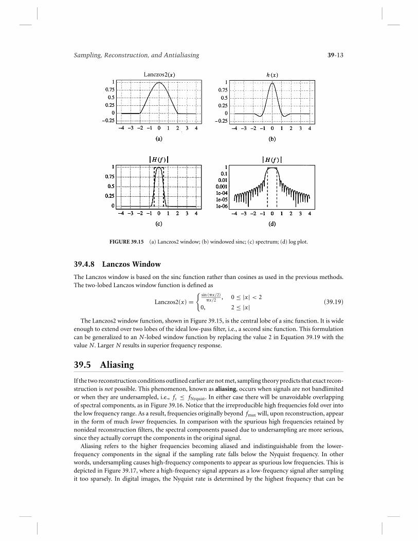
FIGURE 39.15 (a) Lanczos2 window; (b) windowed sinc; (c) spectrum; (d) log plot.

39.4.8 Lanczos Window

The Lanczos window is based on the sinc function rather than cosines as used in the previous methods.The two-lobed Lanczos window function is defined as

Lanczos2(x) ={

sin (�x/2)�x/2 , 0 ≤ |x| < 2

0, 2 ≤ |x| (39.19)

The Lanczos2 window function, shown in Figure 39.15, is the central lobe of a sinc function. It is wideenough to extend over two lobes of the ideal low-pass filter, i.e., a second sinc function. This formulationcan be generalized to an N-lobed window function by replacing the value 2 in Equation 39.19 with thevalue N. Larger N results in superior frequency response.

39.5 Aliasing

If the two reconstruction conditions outlined earlier are not met, sampling theory predicts that exact recon-struction is not possible. This phenomenon, known as aliasing, occurs when signals are not bandlimitedor when they are undersampled, i.e., fs ≤ fNyquist. In either case there will be unavoidable overlappingof spectral components, as in Figure 39.16. Notice that the irreproducible high frequencies fold over intothe low frequency range. As a result, frequencies originally beyond fmax will, upon reconstruction, appearin the form of much lower frequencies. In comparison with the spurious high frequencies retained bynonideal reconstruction filters, the spectral components passed due to undersampling are more serious,since they actually corrupt the components in the original signal.

Aliasing refers to the higher frequencies becoming aliased and indistinguishable from the lower-frequency components in the signal if the sampling rate falls below the Nyquist frequency. In otherwords, undersampling causes high-frequency components to appear as spurious low frequencies. This isdepicted in Figure 39.17, where a high-frequency signal appears as a low-frequency signal after samplingit too sparsely. In digital images, the Nyquist rate is determined by the highest frequency that can be


FIGURE 39.16 Overlapping spectral components give rise to aliasing.

FIGURE 39.17 Aliasing artifacts due to undersampling.

displayed: one cycle every two pixels. Therefore, any attempt to display higher frequencies will producesimilar artifacts.

There is sometimes a misconception in the computer graphics literature that jagged (staircased) edgesare always a symptom of aliasing. This is only partially true. Technically, jagged edges arise from highfrequencies introduced by inadequate reconstruction. Since these high frequencies are not corrupting thelow-frequency components, no aliasing is actually taking place. The confusion lies in that the suggestedremedy of increasing the sampling rate is also used to eliminate aliasing. Of course, the benefit of increasingthe sampling rate is that the replicated spectra are now spaced farther apart from each other. This relaxesthe accuracy constraints for reconstruction filters to perform ideally in the stopband, where they mustsuppress all components beyond some specified cutoff frequency. In this manner, the same nonideal filterswill produce less objectionable output.

It is important to note that a signal may be densely sampled (far above the Nyquist rate) and continueto appear jagged if a zero-order reconstruction filter is used. Box filters used for pixel replication in real-time hardware zooms are a common example of poor reconstruction filters. In this case, the signal isclearly not aliased but rather poorly reconstructed. The distinction between reconstruction and aliasingartifacts becomes clear when we notice that the appearance of jagged edges is improved by blurring. Forexample, it is not uncommon to step back from an image exhibiting excessive blockiness in order to see itmore clearly. This is a defocusing operation that attenuates the high frequencies admitted through nonidealreconstruction. On the other hand, once a signal is truly undersampled, there is no postprocessing possibleto improve its condition. After all, applying an ideal low-pass (reconstruction) filter to a spectrum whosecomponents are already overlapping will only blur the result, not rectify it.

39.6 Antialiasing

The filtering necessary to combat aliasing is known as antialiasing. In order to determine corrective action,we must directly address the two conditions necessary for exact signal reconstruction. The first solution callsfor low-pass filtering before sampling. This method, known as prefiltering, bandlimits the signal to levelsbelow fmax, thereby eliminating the offending high frequencies. Notice that the frequency at which thesignal is to be sampled imposes limits on the allowable bandwidth. This is often necessary when the output


sampling grid must be fixed to the resolution of an output device, e.g., screen resolution. Therefore, aliasingis often a problem that is confronted when a signal is forced to conform to an inadequate resolution dueto physical constraints. As a result, it is necessary to bandlimit, or narrow, the input spectrum to conformto the allotted bandwidth as determined by the sampling frequency.

The second solution is to point-sample at a higher frequency. In doing so, the replicated spectra arespaced farther apart, thereby separating the overlapping spectra tails. This approach theoretically impliessampling at a resolution determined by the highest frequencies present in the signal. Since a surfaceviewed obliquely can give rise to arbitrarily high frequencies, this method may require extremely highresolution. Whereas the first solution adjusts the bandwidth to accommodate the fixed sampling ratefs , the second solution adjusts fs to accommodate the original bandwidth. Antialiasing by samplingat the highest frequency is clearly superior in terms of image quality. This is, of course, operating underdifferent assumptions regarding the possibility of varying fs . In practice, antialiasing is performed througha combination of these two approaches. That is, the sampling frequency is increased so as to reduce theamount of bandlimiting to a minimum.

39.6.1 Point Sampling

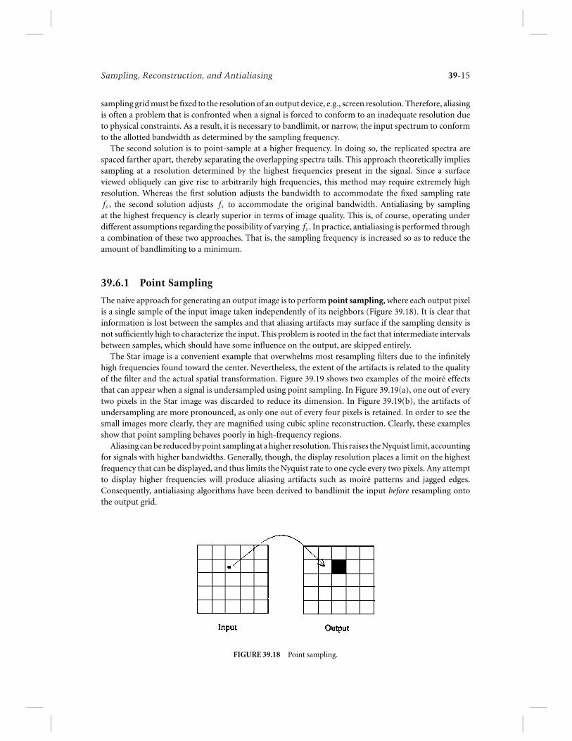
The naive approach for generating an output image is to perform point sampling, where each output pixelis a single sample of the input image taken independently of its neighbors (Figure 39.18). It is clear thatinformation is lost between the samples and that aliasing artifacts may surface if the sampling density isnot sufficiently high to characterize the input. This problem is rooted in the fact that intermediate intervalsbetween samples, which should have some influence on the output, are skipped entirely.

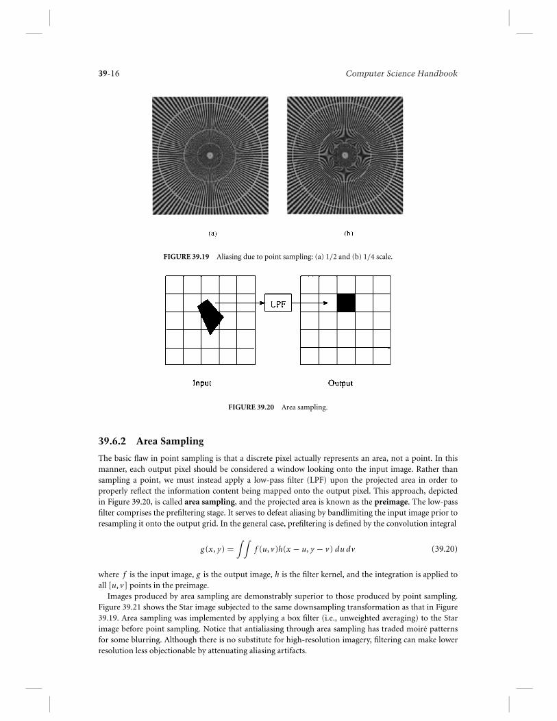
The Star image is a convenient example that overwhelms most resampling filters due to the infinitelyhigh frequencies found toward the center. Nevertheless, the extent of the artifacts is related to the qualityof the filter and the actual spatial transformation. Figure 39.19 shows two examples of the moire effectsthat can appear when a signal is undersampled using point sampling. In Figure 39.19(a), one out of everytwo pixels in the Star image was discarded to reduce its dimension. In Figure 39.19(b), the artifacts ofundersampling are more pronounced, as only one out of every four pixels is retained. In order to see thesmall images more clearly, they are magnified using cubic spline reconstruction. Clearly, these examplesshow that point sampling behaves poorly in high-frequency regions.

Aliasing can be reduced by point sampling at a higher resolution. This raises the Nyquist limit, accountingfor signals with higher bandwidths. Generally, though, the display resolution places a limit on the highestfrequency that can be displayed, and thus limits the Nyquist rate to one cycle every two pixels. Any attemptto display higher frequencies will produce aliasing artifacts such as moire patterns and jagged edges.Consequently, antialiasing algorithms have been derived to bandlimit the input before resampling ontothe output grid.

FIGURE 39.18 Point sampling.


FIGURE 39.19 Aliasing due to point sampling: (a) 1/2 and (b) 1/4 scale.

FIGURE 39.20 Area sampling.

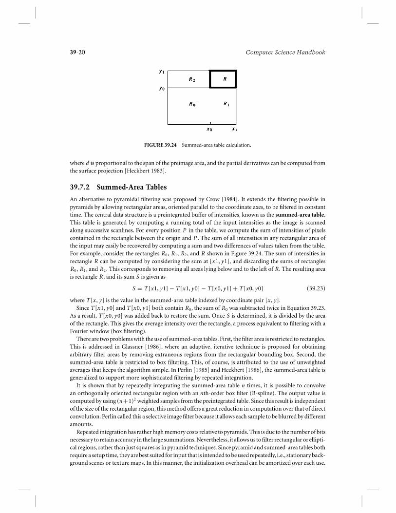
39.6.2 Area Sampling

The basic flaw in point sampling is that a discrete pixel actually represents an area, not a point. In thismanner, each output pixel should be considered a window looking onto the input image. Rather thansampling a point, we must instead apply a low-pass filter (LPF) upon the projected area in order toproperly reflect the information content being mapped onto the output pixel. This approach, depictedin Figure 39.20, is called area sampling, and the projected area is known as the preimage. The low-passfilter comprises the prefiltering stage. It serves to defeat aliasing by bandlimiting the input image prior toresampling it onto the output grid. In the general case, prefiltering is defined by the convolution integral

g (x , y) =∫ ∫

f (u, v)h(x − u, y − v) du dv (39.20)

where f is the input image, g is the output image, h is the filter kernel, and the integration is applied toall [u, v] points in the preimage.

Images produced by area sampling are demonstrably superior to those produced by point sampling.Figure 39.21 shows the Star image subjected to the same downsampling transformation as that in Figure39.19. Area sampling was implemented by applying a box filter (i.e., unweighted averaging) to the Starimage before point sampling. Notice that antialiasing through area sampling has traded moire patternsfor some blurring. Although there is no substitute for high-resolution imagery, filtering can make lowerresolution less objectionable by attenuating aliasing artifacts.


FIGURE 39.21 Aliasing due to area sampling: (a) 1/2 and (b) 1/4 scale.

FIGURE 39.22 Supersampling.

39.6.3 Supersampling

The process of using more than one regularly spaced sample per pixel is known as supersampling. Eachoutput pixel value is evaluated by computing a weighted average of the samples taken from their respectivepreimages. For example, if the supersampling grid is three times denser than the output grid (i.e., thereare nine grid points per pixel area), each output pixel will be an average of the nine samples taken from itsprojection in the input image. If, say, three samples hit a green object and the remaining six samples hit ablue object, the composite color in the output pixel will be one-third green and two-thirds blue, assuminga box filter is used.

Supersampling reduces aliasing by bandlimiting the input signal. The purpose of the high-resolutionsupersampling grid is to refine the estimate of the preimages seen by the output pixels. The samples thenenter the prefiltering stage, consisting of a low-pass filter. This permits the input to be resampled ontothe (relatively) low-resolution output grid without any offending high frequencies introducing aliasingartifacts. In Figure 39.22 we see an output pixel subdivided into nine subpixel samples which each undergoinverse mapping, sampling the input at nine positions. Those nine values then pass through a low-passfilter to be averaged into a single output value.

Supersampling was used to achieve antialiasing in Figure 39.1 for pixels near the horizon. There are twoproblems, however, associated with straightforward supersampling. The first problem is that the newlydesignated high frequency of the prefiltered image continues to be fixed. Therefore, there will always besufficiently higher frequencies that will alias. The second problem is cost. In our example, supersamplingwill take nine times longer than point sampling. Although there is a clear need for the additional compu-tation, the dense placement of samples can be optimized. Adaptive supersampling is introduced to addressthese drawbacks.


39.6.4 Adaptive Supersampling

In adaptive supersampling, the samples are distributed more densely in areas of high intensity variance.In this manner, supersamples are collected only in regions that warrant their use. Early work in adaptivesupersampling for computer graphics is described in Whitted [1980]. The strategy is to subdivide areasbetween previous samples when an edge, or some other high-frequency pattern, is present. Two approachesto adaptive supersampling have been described in the literature. The first approach allows sampling densityto vary as a function of local image variance [Lee et al. 1985, Kajiya 1986]. A second approach introducestwo levels of sampling densities: a regular pattern for most areas and a higher-density pattern for regionsdemonstrating high frequencies. The regular pattern simply consists of one sample per output pixel. Thehigh density pattern involves local supersampling at a rate of 4 to 16 samples per pixel. Typically, theserates are adequate for suppressing aliasing artifacts.

A strategy is required to determine where supersampling is necessary. In Mitchell [1987], the authordescribes a method in which the image is divided into small square supersampling cells, each containingeight or nine of the low-density samples. The entire cell is supersampled if its samples exhibit excessivevariation. In Lee et al. [1985], the variance of the samples is used to indicate high frequency. It is well known,however, that variance is a poor measure of visual perception of local variation. Another alternative is touse contrast, which more closely models the nonlinear response of the human eye to rapid fluctuations inlight intensities [Caelli 1981]. Contrast is given as

C = Imax − Imin

Imax + Imin(39.21)

Adaptive sampling reduces the number of samples required for a given image quality. The problem withthis technique, however, is that the variance measurement is itself based on point samples, and so thismethod can fail as well. This is particularly true for subpixel objects that do not cross pixel boundaries.Nevertheless, adaptive sampling presents a far more reliable and cost-effective alternative to supersampling.

39.7 Prefiltering

Area sampling can be accelerated if constraints on the filter shape are imposed. Pyramids and preinte-grated tables are introduced to approximate the convolution integral with a constant number of accesses.This compares favorably against direct convolution, which requires a large number of samples that growproportionately to preimage area. As we shall see, though, the filter area will be limited to squares orrectangles, and the kernel will consist of a box filter. Subsequent advances have extended their use to moregeneral cases with only marginal increases in cost.

39.7.1 Pyramids

Pyramids are multiresolution data structures commonly used in image processing and computer vision.They are generated by successively bandlimiting and subsampling the original image to form a hierarchyof images at ever decreasing resolutions. The original image serves as the base of the pyramid, and itscoarsest version resides at the apex. Thus, in a lower-resolution version of the input, each pixel representsthe average of some number of pixels in the higher-resolution version.

The resolution of successive levels typically differs by a power of two. This means that successivelycoarser versions each have one-quarter of the total number of pixels as their adjacent predecessors. Thememory cost of this organization is modest: 1+1/4+1/16+· · · = 4/3 times that needed for the originalinput. This requires only 33% more memory.

To filter a preimage, one of the pyramid levels is selected based on the size of its bounding square box.That level is then point sampled and assigned to the respective output pixel. The primary benefit of thisapproach is that the cost of the filter is constant, requiring the same number of pixel accesses independentof the filter size. This performance gain is the result of the filtering that took place while creating the


FIGURE 39.23 Mip-map memory organization.

pyramid. Furthermore, if preimage areas are adequately approximated by squares, the direct convolutionmethods amount to point-sampling a pyramid. This approach was first applied to texture mapping inCatmull [1974] and described in Dungan et al. [1978].

There are several problems with the use of pyramids. First, the appropriate pyramid level must beselected. A coarse level may yield excessive blur, while the adjacent finer level may be responsible foraliasing due to insufficient bandlimiting. Second, preimages are constrained to be squares. This provesto be a crude approximation for elongated preimages. For example, when a surface is viewed obliquelythe texture may be compressed along one dimension. Using the largest bounding square will include thecontributions of many extraneous samples and result in excessive blur. These two issues were addressedin Williams [1983] and Crow [1984], respectively, along with extensions proposed by other researchers.

Williams proposed a pyramid organization called mip map to store color images at multiple resolutionsin a convenient memory organization [Williams 1983]. The acronym “mip” stands for “multum in parvo,”a Latin phrase meaning “much in little.” The scheme supports trilinear interpolation, where both intra-and interlevel interpolation can be computed using three normalized coordinates: u, v , and d . Both u andv are spatial coordinates used to access points within a pyramid level. The d coordinate is used to index,and interpolate between, different levels of the pyramid. This is depicted in Figure 39.23.

The quadrants touching the east and south borders contain the original red, green, and blue (RGB)components of the color image. The remaining upper left quadrant contains all the lower-resolution copiesof the original. The memory organization depicted in Figure 39.23 clearly supports the earlier claim thatthe memory cost is 4/3 times that required for the original input. Each level is shown indexed by the[u, v , d] coordinate system, where d is shown slicing through the pyramid levels. Since correspondingpoints in different pyramid levels have indices which are related by some power of two, simple binary shiftscan be used to access these points across the multiresolution copies. This is a particularly attractive featurefor hardware implementation.

The primary difference between mip maps and ordinary pyramids is the trilinear interpolation schemepossible with the [u, v , d] coordinate system. Since they allow a continuum of points to be accessed, mipmaps are referred to as pyramidal parametric data structures. In Williams’s implementation, a box filter wasused to create the mip maps, and a triangle filter was used to perform intra- and interlevel interpolation.The value of d must be chosen to balance the tradeoff between aliasing and blurring. Heckbert suggests

d2 = max

((∂u

∂x

)2

+(

∂v

∂x

)2

,

(∂u

∂y

)2

+(

∂v

∂y

)2)(39.22)


FIGURE 39.24 Summed-area table calculation.

where d is proportional to the span of the preimage area, and the partial derivatives can be computed fromthe surface projection [Heckbert 1983].

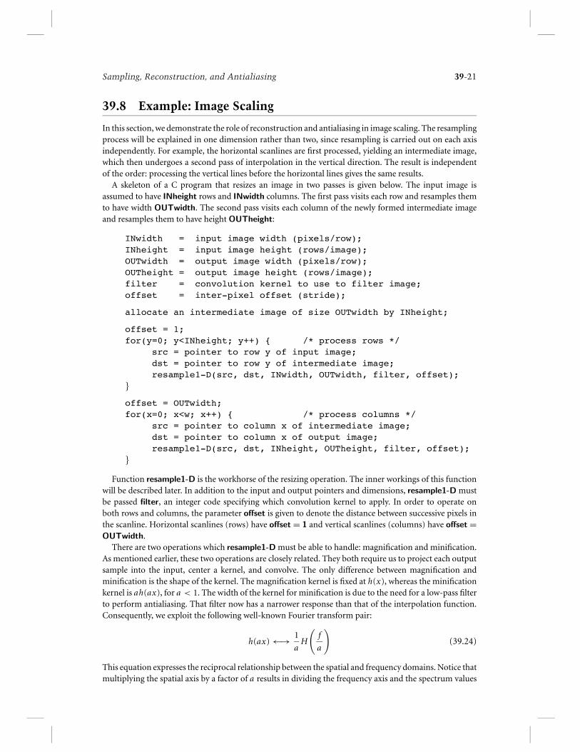
39.7.2 Summed-Area Tables

An alternative to pyramidal filtering was proposed by Crow [1984]. It extends the filtering possible inpyramids by allowing rectangular areas, oriented parallel to the coordinate axes, to be filtered in constanttime. The central data structure is a preintegrated buffer of intensities, known as the summed-area table.This table is generated by computing a running total of the input intensities as the image is scannedalong successive scanlines. For every position P in the table, we compute the sum of intensities of pixelscontained in the rectangle between the origin and P . The sum of all intensities in any rectangular area ofthe input may easily be recovered by computing a sum and two differences of values taken from the table.For example, consider the rectangles R0, R1, R2, and R shown in Figure 39.24. The sum of intensities inrectangle R can be computed by considering the sum at [x1, y1], and discarding the sums of rectanglesR0, R1, and R2. This corresponds to removing all areas lying below and to the left of R. The resulting areais rectangle R, and its sum S is given as

S = T[x1, y1] − T[x1, y0] − T[x0, y1] + T[x0, y0] (39.23)

where T[x , y] is the value in the summed-area table indexed by coordinate pair [x , y].Since T[x1, y0] and T[x0, y1] both contain R0, the sum of R0 was subtracted twice in Equation 39.23.

As a result, T[x0, y0] was added back to restore the sum. Once S is determined, it is divided by the areaof the rectangle. This gives the average intensity over the rectangle, a process equivalent to filtering with aFourier window (box filtering).

There are two problems with the use of summed-area tables. First, the filter area is restricted to rectangles.This is addressed in Glassner [1986], where an adaptive, iterative technique is proposed for obtainingarbitrary filter areas by removing extraneous regions from the rectangular bounding box. Second, thesummed-area table is restricted to box filtering. This, of course, is attributed to the use of unweightedaverages that keeps the algorithm simple. In Perlin [1985] and Heckbert [1986], the summed-area table isgeneralized to support more sophisticated filtering by repeated integration.

It is shown that by repeatedly integrating the summed-area table n times, it is possible to convolvean orthogonally oriented rectangular region with an nth-order box filter (B-spline). The output value iscomputed by using (n+1)2 weighted samples from the preintegrated table. Since this result is independentof the size of the rectangular region, this method offers a great reduction in computation over that of directconvolution. Perlin called this a selective image filter because it allows each sample to be blurred by differentamounts.

Repeated integration has rather high memory costs relative to pyramids. This is due to the number of bitsnecessary to retain accuracy in the large summations. Nevertheless, it allows us to filter rectangular or ellipti-cal regions, rather than just squares as in pyramid techniques. Since pyramid and summed-area tables bothrequire a setup time, they are best suited for input that is intended to be used repeatedly, i.e., stationary back-ground scenes or texture maps. In this manner, the initialization overhead can be amortized over each use.


39.8 Example: Image Scaling

In this section, we demonstrate the role of reconstruction and antialiasing in image scaling. The resamplingprocess will be explained in one dimension rather than two, since resampling is carried out on each axisindependently. For example, the horizontal scanlines are first processed, yielding an intermediate image,which then undergoes a second pass of interpolation in the vertical direction. The result is independentof the order: processing the vertical lines before the horizontal lines gives the same results.

A skeleton of a C program that resizes an image in two passes is given below. The input image isassumed to have INheight rows and INwidth columns. The first pass visits each row and resamples themto have width OUTwidth. The second pass visits each column of the newly formed intermediate imageand resamples them to have height OUTheight:

INwidth = input image width (pixels/row);INheight = input image height (rows/image);OUTwidth = output image width (pixels/row);OUTheight = output image height (rows/image);filter = convolution kernel to use to filter image;offset = inter-pixel offset (stride);

allocate an intermediate image of size OUTwidth by INheight;

offset = 1;for(y=0; y<INheight; y++) { /* process rows */

src = pointer to row y of input image;dst = pointer to row y of intermediate image;resample1-D(src, dst, INwidth, OUTwidth, filter, offset);

}

offset = OUTwidth;for(x=0; x<w; x++) { /* process columns */

src = pointer to column x of intermediate image;dst = pointer to column x of output image;resample1-D(src, dst, INheight, OUTheight, filter, offset);

}

Function resample1-D is the workhorse of the resizing operation. The inner workings of this functionwill be described later. In addition to the input and output pointers and dimensions, resample1-D mustbe passed filter, an integer code specifying which convolution kernel to apply. In order to operate onboth rows and columns, the parameter offset is given to denote the distance between successive pixels inthe scanline. Horizontal scanlines (rows) have offset = 1 and vertical scanlines (columns) have offset =OUTwidth.

There are two operations which resample1-D must be able to handle: magnification and minification.As mentioned earlier, these two operations are closely related. They both require us to project each outputsample into the input, center a kernel, and convolve. The only difference between magnification andminification is the shape of the kernel. The magnification kernel is fixed at h(x), whereas the minificationkernel is ah(ax), for a < 1. The width of the kernel for minification is due to the need for a low-pass filterto perform antialiasing. That filter now has a narrower response than that of the interpolation function.Consequently, we exploit the following well-known Fourier transform pair:

h(ax) ←→ 1

aH

(f

a

)(39.24)

This equation expresses the reciprocal relationship between the spatial and frequency domains. Notice thatmultiplying the spatial axis by a factor of a results in dividing the frequency axis and the spectrum values


by that same factor. Since we want the spectrum values to be left intact, we use ah(ax) as the convolutionkernel for blurring, where a > 1. This implies that the shape of the kernel changes as a function of scalefactor when we are downsampling the input. This was not the case for magnification.

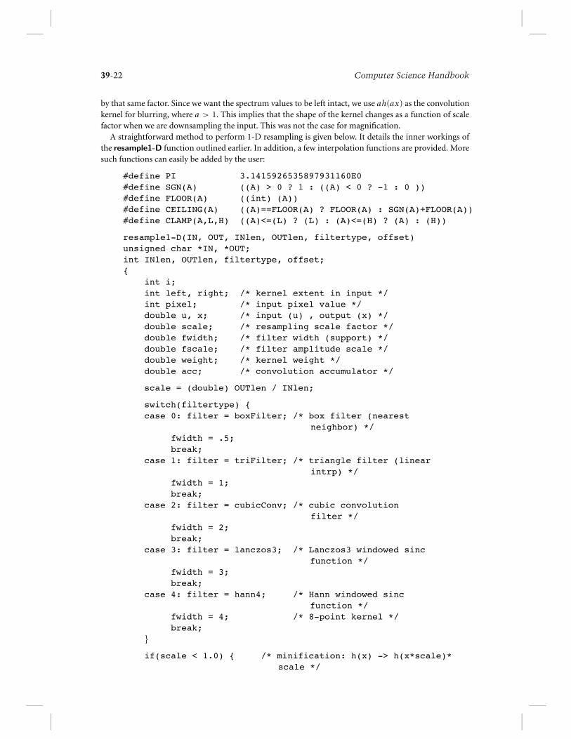
A straightforward method to perform 1-D resampling is given below. It details the inner workings ofthe resample1-D function outlined earlier. In addition, a few interpolation functions are provided. Moresuch functions can easily be added by the user:

#define PI 3.1415926535897931160E0#define SGN(A) ((A) > 0 ? 1 : ((A) < 0 ? -1 : 0 ))#define FLOOR(A) ((int) (A))#define CEILING(A) ((A)==FLOOR(A) ? FLOOR(A) : SGN(A)+FLOOR(A))#define CLAMP(A,L,H) ((A)<=(L) ? (L) : (A)<=(H) ? (A) : (H))

resample1-D(IN, OUT, INlen, OUTlen, filtertype, offset)unsigned char *IN, *OUT;int INlen, OUTlen, filtertype, offset;{

int i;int left, right; /* kernel extent in input */int pixel; /* input pixel value */double u, x; /* input (u) , output (x) */double scale; /* resampling scale factor */double fwidth; /* filter width (support) */double fscale; /* filter amplitude scale */double weight; /* kernel weight */double acc; /* convolution accumulator */

scale = (double) OUTlen / INlen;

switch(filtertype) {case 0: filter = boxFilter; /* box filter (nearest

neighbor) */fwidth = .5;break;

case 1: filter = triFilter; /* triangle filter (linearintrp) */

fwidth = 1;break;

case 2: filter = cubicConv; /* cubic convolutionfilter */

fwidth = 2;break;

case 3: filter = lanczos3; /* Lanczos3 windowed sincfunction */

fwidth = 3;break;

case 4: filter = hann4; /* Hann windowed sincfunction */

fwidth = 4; /* 8-point kernel */break;

}

if(scale < 1.0) { /* minification: h(x) -> h(x*scale)*scale */


fwidth = fwidth / scale; /* broaden filter */fscale = scale; /* lower amplitude */

} else fscale = 1.0;

/* project each output pixel to input, center kernel, andconvolve */for(x=0; x<OUTlen; x++) {

/* map output x to input u: inverse mapping */u = x / scale;

/* left and right extent of kernel centered at u */if(u - fwidth < 0) {

left = FLOOR (u - fwidth);else left = CEILING(u - fwidth);right = FLOOR(u + fwidth);

/* reset acc for collecting convolution products */acc = 0;

/* weigh input pixels around u with kernel */for(i=left; i <= right; i++) {

pixel = IN[ CLAMP(i, 0, INlen-1)*offset];weight = (*filter)((u - i) * fscale);acc += (pixel * weight);

}

/* assign weighted accumulator to OUT */OUT[x*offset] = acc * fscale;

}}

/* ~~~~~~~~~~~~~~~~~~~~~~~~~~~~~~~~~~~~~~~~~~~~~~~~~~~~~~~~~~~~

* boxFilter:** Box (nearest neighbor) filter.*/

doubleboxFilter(t)double t;{

if((t > -.5) && (t <= .5)) return(1.0);return(0.0);

}

/* ~~~~~~~~~~~~~~~~~~~~~~~~~~~~~~~~~~~~~~~~~~~~~~~~~~~~~~~~~~~~

* triFilter:** Triangle filter (used for linear interpolation).*/

doubletriFilter(t)double t;{

if(t < 0) t = -t;if(t < 1.0) return(1.0 - t);


return(0.0);}

/* ~~~~~~~~~~~~~~~~~~~~~~~~~~~~~~~~~~~~~~~~~~~~~~~~~~~~~~~~~~~~

* cubicConv:** Cubic convolution filter.*/

doublecubicConv(t)double t;{

double A, t2, t3;

if(t < 0) t = -t;t2 = t * t;t3 = t2 * t;

A = -1.0; /* user-specified free parameter */if(t < 1.0) return((A+2)*t3 - (A+3)*t2 + 1);if(t < 2.0) return(A*(t3 - 5*t2 + 8*t - 4));return(0.0);

}

/* ~~~~~~~~~~~~~~~~~~~~~~~~~~~~~~~~~~~~~~~~~~~~~~~~~~~~~~~~~~~~

* sinc:** Sinc function.*/

doublesinc(t)double t;{

t *= PI;if(t != 0) return(sin(t) / t);return(1.0);

}

/* ~~~~~~~~~~~~~~~~~~~~~~~~~~~~~~~~~~~~~~~~~~~~~~~~~~~~~~~~~~~~

* lanczos3:** Lanczos3 filter.*/

doublelanczos3(t)double t;{

if(t < 0) t = -t;if(t < 3.0) return(sinc(t) * sinc(t/3.0));return(0.0);

}

/* ~~~~~~~~~~~~~~~~~~~~~~~~~~~~~~~~~~~~~~~~~~~~~~~~~~~~~~~~~~~~

* hann:


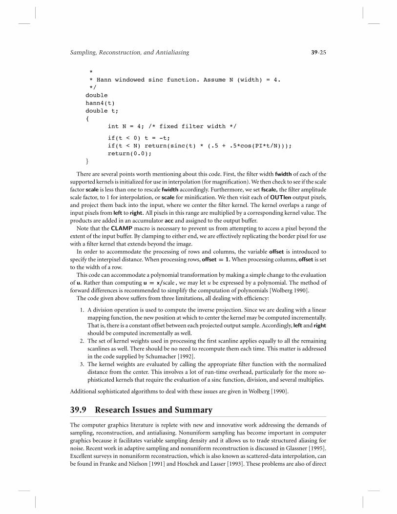
** Hann windowed sinc function. Assume N (width) = 4.*/

doublehann4(t)double t;{

int N = 4; /* fixed filter width */

if(t < 0) t = -t;if(t < N) return(sinc(t) * (.5 + .5*cos(PI*t/N)));return(0.0);

}

There are several points worth mentioning about this code. First, the filter width fwidth of each of thesupported kernels is initialized for use in interpolation (for magnification). We then check to see if the scalefactor scale is less than one to rescale fwidth accordingly. Furthermore, we set fscale, the filter amplitudescale factor, to 1 for interpolation, or scale for minification. We then visit each of OUTlen output pixels,and project them back into the input, where we center the filter kernel. The kernel overlaps a range ofinput pixels from left to right. All pixels in this range are multiplied by a corresponding kernel value. Theproducts are added in an accumulator acc and assigned to the output buffer.

Note that the CLAMP macro is necessary to prevent us from attempting to access a pixel beyond theextent of the input buffer. By clamping to either end, we are effectively replicating the border pixel for usewith a filter kernel that extends beyond the image.

In order to accommodate the processing of rows and columns, the variable offset is introduced tospecify the interpixel distance. When processing rows, offset = 1. When processing columns, offset is setto the width of a row.

This code can accommodate a polynomial transformation by making a simple change to the evaluationof u. Rather than computing u = x/scale , we may let u be expressed by a polynomial. The method offorward differences is recommended to simplify the computation of polynomials [Wolberg 1990].

The code given above suffers from three limitations, all dealing with efficiency:

1. A division operation is used to compute the inverse projection. Since we are dealing with a linearmapping function, the new position at which to center the kernel may be computed incrementally.That is, there is a constant offset between each projected output sample. Accordingly, left and right

should be computed incrementally as well.2. The set of kernel weights used in processing the first scanline applies equally to all the remaining

scanlines as well. There should be no need to recompute them each time. This matter is addressedin the code supplied by Schumacher [1992].

3. The kernel weights are evaluated by calling the appropriate filter function with the normalizeddistance from the center. This involves a lot of run-time overhead, particularly for the more so-phisticated kernels that require the evaluation of a sinc function, division, and several multiplies.

Additional sophisticated algorithms to deal with these issues are given in Wolberg [1990].

39.9 Research Issues and Summary

The computer graphics literature is replete with new and innovative work addressing the demands ofsampling, reconstruction, and antialiasing. Nonuniform sampling has become important in computergraphics because it facilitates variable sampling density and it allows us to trade structured aliasing fornoise. Recent work in adaptive sampling and nonuniform reconstruction is discussed in Glassner [1995].Excellent surveys in nonuniform reconstruction, which is also known as scattered-data interpolation, canbe found in Franke and Nielson [1991] and Hoschek and Lasser [1993]. These problems are also of direct


consequence to image compression. The ability to determine a unique minimal set of samples to completelyrepresent a signal within some specified error tolerance remains an active area of research. The solutionmust be closely coupled with a nonuniform reconstruction method. Although traditional reconstructionmethods are well understood within the framework described in this chapter, the analysis of nonuniformsampling and reconstruction remains challenging.

We now summarize the basic principles of sampling theory, reconstruction, and antialiasing that havebeen presented in this chapter. We have shown that a continuous signal may be reconstructed fromits samples if the signal is bandlimited and the sampling frequency exceeds the Nyquist rate. These arethe two necessary conditions for image reconstruction to be possible. Since sampling can be shown toreplicate a signal’s spectrum across the frequency domain, ideal low-pass filtering was introduced as ameans of retaining the original spectrum while discarding its copies. Unfortunately, the ideal low-passfilter in the spatial domain is an infinitely wide sinc function. Since this is difficult to work with, nonidealreconstruction filters are introduced to approximate the reconstructed output. These filters are nonideal inthe sense that they do not completely attenuate the spectra copies. Furthermore, they contribute to someblurring of the original spectrum. In general, poor reconstruction leads to artifacts such as jagged edges.

Aliasing refers to the phenomenon that occurs when a signal is undersampled. This happens if thereconstruction conditions mentioned above are violated. In order to resolve this problem, one of twoactions may be taken. Either the signal can be bandlimited to a range that complies with the samplingfrequency, or the sampling frequency can be increased. In practice, some combination of both options istaken, leaving some relatively unobjectionable aliasing in the output.

Examples of the concepts discussed thus are concisely depicted in Figure 39.25 through 39.27. They at-tempt to illustrate the effects of sampling and low-pass filtering on the quality of the reconstructed signal andits spectrum. The first row of Figure 39.25 shows a signal and its spectrum, bandlimited to 0.5 cycle/pixel.For pedagogical purposes, we treat this signal as if it were continuous. In actuality, though, it is a 256-sample horizontal cross section taken from a digital image. Since each pixel has four samples contributingto it, there is a maximum of two cycles per pixel. The horizontal axes of the spectrum account for this fact.

The second row shows the effect of sampling the signal. Since fs = 1 sample/pixel, there are four copiesof the baseband spectrum in the range shown. Each copy is scaled by fs = 1, leaving the magnitudesintact. In the third row, the 64 samples are shown convolved with a sinc function in the spatial domain.This corresponds to a rectangular pulse in the frequency domain. Since the sinc function is used here forimage reconstruction, it must have an amplitude of unity value in order to interpolate the data. This forcesthe height of the rectangular pulse in the frequency domain to vary in response to fs .

A few comments on the reciprocal relationship between the spatial and frequency domains are in orderhere, particularly as they apply to the ideal low-pass filter. We again refer to the variables A and W as thesinc amplitude and bandwidth. As a sinc function is made broader, the value 1/2W is made to change, sinceW is decreasing to accommodate zero crossings at larger intervals. Accordingly, broader sinc functionscause more blurring, and their spectra reflect this by reducing the cutoff frequency to some smaller W.Conversely, narrower sinc functions cause less blurring, and W takes on some larger value. In eithercase, the amplitude of the sinc function or its spectrum will change. That is, we can fix the amplitude ofthe sinc function so that only the rectangular pulse of the spectrum changes height A/2W as W varies.Alternatively, we can fix A/2W to remain constant as W changes, forcing us to vary A. The choice dependson the application.

When the sinc function is used to interpolate data, it is necessary to fix A to 1. Therefore, as the samplingdensity changes, the positions of the zero crossings shift, causing W to vary. This makes the amplitude ofthe spectrum’s rectangular pulse change. On the other hand, if the sinc function is applied to bandlimit, notinterpolate, the input signal, then it is important to fix A/2W to 1 so that the passband frequencies remainintact. Since W is once again varying, A must change proportionately to keep A/2W constant. Therefore,this application of the ideal low-pass filter requires the amplitude of the sinc function to be responsive to W.

In the examples presented below, our objective is to interpolate (reconstruct) the input, and so A = 1regardless of the sampling density. Consequently, the height of the spectrum of the reconstruction filterchanges. To make the Fourier transforms of the filters easier to see, we have not drawn the frequency


FIGURE 39.25 Sampling and reconstruction (with an adequate sampling rate).

response of the reconstruction filters to scale. Therefore, the rectangular pulse function in the third row ofFigure 39.25 actually has height A/2W = 1. The fourth row of the figure shows the result after applying theideal low-pass filter. As sampling theory predicts, the output is identical to the original signal. The last tworows of the figure illustrate the consequences of nonideal reconstruction filtering. Instead of using a sincfunction, a triangle function corresponding to linear interpolation was applied. In the frequency domainthis corresponds to the square of the sinc function. Not surprisingly, the spectrum of the reconstructedsignal suffers in both the passband and the stopband.

The identical sequence of filtering operations is performed in Figure 39.26. In this figure, though,the sampling rate has been lowered to fs = 0.5, meaning that only one sample is collected for every


FIGURE 39.26 Sampling and reconstruction (with an inadequate sampling rate).

two output pixels. Consequently, the replicated spectra are multiplied by 0.5, leaving the magnitudes at4. Unfortunately, this sampling rate causes the replicated spectra to overlap. This, in turn, gives rise toaliasing, as depicted in the fourth row of the figure. Applying the triangle function to perform linearinterpolation also yields poor results.

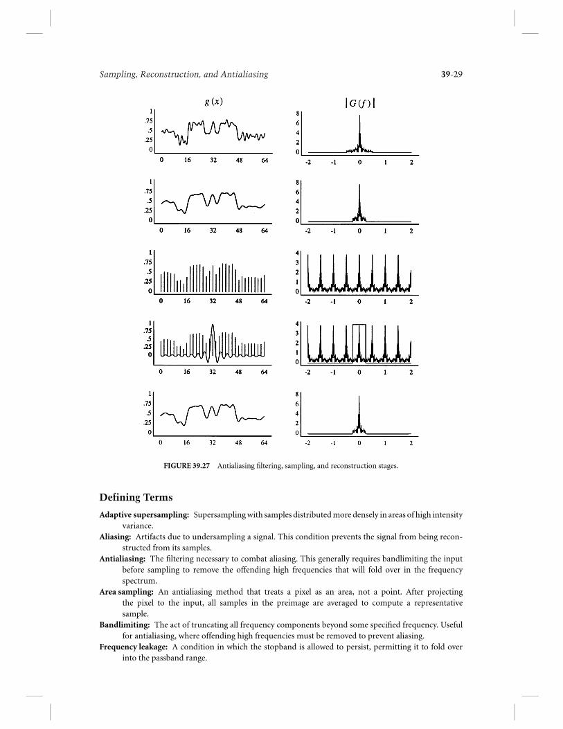
In order to combat these artifacts, the input signal must be bandlimited to accommodate the lowsampling rate. This is shown in the second row of Figure 39.27, where we see that all frequencies beyondW = 0.25 are truncated. This causes the input signal to be blurred. In this manner we have traded aliasingfor blurring, a far less objectionable artifact. Sampling this function no longer causes the replicated copiesto overlap. Convolving with an ideal low-pass filter now properly isolates the bandlimited spectrum.


FIGURE 39.27 Antialiasing filtering, sampling, and reconstruction stages.

Defining Terms

Adaptive supersampling: Supersampling with samples distributed more densely in areas of high intensityvariance.

Aliasing: Artifacts due to undersampling a signal. This condition prevents the signal from being recon-structed from its samples.

Antialiasing: The filtering necessary to combat aliasing. This generally requires bandlimiting the inputbefore sampling to remove the offending high frequencies that will fold over in the frequencyspectrum.

Area sampling: An antialiasing method that treats a pixel as an area, not a point. After projectingthe pixel to the input, all samples in the preimage are averaged to compute a representativesample.

Bandlimiting: The act of truncating all frequency components beyond some specified frequency. Usefulfor antialiasing, where offending high frequencies must be removed to prevent aliasing.

Frequency leakage: A condition in which the stopband is allowed to persist, permitting it to fold overinto the passband range.


Gibbs phenomenon: Overshoots and undershoots caused by reconstructing a signal with truncated fre-quency components.

Nyquist rate: The minimum sampling frequency. It is twice the maximum signal frequency.Passband: Consists of all frequencies that must be retained by the applied filter.Point sampling: Each output pixel is a single sample of the input image. This approach generally leads to

aliasing because a pixel is treated as a point, not an area.Prefilter: The low-pass filter (blurring) applied to achieve antialiasing by bandlimiting the input image

prior to resampling it onto the output grid.Preimage: The projected area of an output pixel as it is mapped to the input image.Pyramid: A multiresolution data structure generated by successively bandlimiting and subsampling the

original image to form a hierarchy of images at ever decreasing resolutions. Useful for acceleratingantialiasing. Filtering limited to square regions and unweighted averaging.

Reconstruction: The act of recovering a continuous signal from its samples. Interpolation.Stopband: Consists of all frequencies that must be suppressed by the applied filter.Summed-area table: Preintegrated buffer of intensities generated by computing a running total of the in-

put intensities as the image is scanned along successive scanlines. Useful for accelerating antialiasing.Filtering limited to rectangular regions and unweighted averaging.

Supersampling: An antialiasing method that collects more than one regularly spaced sample per pixel.

References

Antoniou, A. 1979. Digital Filters: Analysis and Design. McGraw–Hill, New York.Caelli, T. 1981. Visual Perception: Theory and Practice. Pergamon Press, Oxford.Castleman, K. 1996. Digital Image Processing. Prentice–Hall, Englewood Cliffs, NJ.Catmull, E. 1974. A Subdivision Algorithm for Computer Display of Curved Surfaces. Ph.D. thesis, Depart-

ment of Computer Science, University of Utah. Tech. Rep. UTEC-CSc-74-133.Crow, F. C. 1984. Summed-area tables for texture mapping. Comput. Graphics (Proc. SIGGRAPH)

18(3):207–212.Dungan, W., Jr., Stenger, A., and Sutty, G. 1978. Texture tile considerations for raster graphics. Comput.

Graphics. (Proc. SIGGRAPH) 12(3):130–134.Fant, K. M. 1986. A nonaliasing, real-time spatial transform technique. IEEE Comput. Graphics Appl.

6(1):71–80.Franke, R. and Nielson, G. M. 1991. Scattered data interpolation and applications: a tutorial and survey.

In Geometric Modelling: Methods and Their Application. H. Hagen and D. Roller, eds., pp. 131–160.Springer–Verlag, Berlin.

Glassner, A. 1986. Adaptive precision in texture mapping. Comput. Graphics (Proc. SIGGRAPH) 20(4):297–306.

Glassner, A. 1995. Principles of Digital Image Synthesis. Morgan Kaufmann, San Francisco.Gonzalez, R. C. and Woods, R. 1992. Digital Image Processing. Addison–Wesley, Reading, MA.Heckbert, P. 1983. Texture mapping polygons in perspective. Tech. Memo 13, NYIT Computer Graphics

Lab.Heckbert, P. 1986. Filtering by repeated integration. Comput. Graphics (Proc. SIGGRAPH) 20(4):315–321.Hoschek, J. and Lasser, D. 1993. Computer Aided Geometric Design. A K Peters, Wellesley, MA.Jain, A. K. 1989. Fundamentals of Digital Image Processing. Prentice–Hall, Englewood Cliffs, NJ.Kajiya, J. 1986. The Rendering Equation. Comput. Graphics Proc., SIGGRAPH 20(4):143–150.Lee, M., Redner, R. A., and Uselton, S. P. 1985. Statistically optimized sampling for distributed ray tracing.

Comput. Graphics (Proc. SIGGRAPH) 19(3):61–67.Mitchell, D. P. 1987. Generating antialiased images at low sampling densities. Comput. Graphics (Proc.

SIGGRAPH) 21(4):65–72.Mitchell, D. P. and Netravali, A. N. 1988. Reconstruction filters in computer graphics. Comput. Graphics

(Proc. SIGGRAPH) 22(4):221–228.


Perlin, K. 1985. Course notes. SIGGRAPH’85 State of the Art in Image Synthesis Seminar Notes.Pratt, W. K. 1991. Digital Image Processing, 2nd ed. J. Wiley, New York.Russ, J. C. 1992. The Image Processing Handbook. CRC Press, Boca Raton, FL.Schumacher, D. 1992. General filtered image rescaling. In Graphics Gems III. David Kirk, Ed., Academic

Press, New York.Shannon, C.E. 1948. A mathematical theory of communication. Bell System Tech. J. 27:379–423 (July

1948), 27:623–656 (Oct. 1948).Shannon, C. E. 1949. Communication in the presence of noise. Proc. Inst. Radio Eng. 37(1):10–21.Whitted, T. 1980. An improved illumination model for shaded display. Commun. ACM 23(6):343–349.Williams, L. 1983. Pyramidal parametrics. Comput. Graphics (Proc. SIGGRAPH) 17(3):1–11.Wolberg, G. 1990. Digital Image Warping. IEEE Comput. Soc. Press, Los Alamitos, CA.

Further Information

The material contained in this chapter was drawn from Wolberg [1990]. Additional image processing textsthat offer a comprehensive treatment of sampling, reconstruction, and antialiasing include Castleman[1996], Glassner [1995], Gonzalez and Woods [1992], Jain [1989], Pratt [1991], and Russ [1992].

Advances in the field are reported in several journals, including IEEE Transactions on Image Processing,IEEE Transactions on Signal Processing, IEEE Transactions on Acoustics, Speech, and Signal Processing, andGraphical Models and Image Processing. Related work in computer graphics is also reported in ComputerGraphics (ACM SIGGRAPH Proceedings), IEEE Computer Graphics and Applications, and IEEE Transactionson Visualization and Computer Graphics.

Documents

Sampling, Reconstruction, and Antialiasingwolberg/pub/crc04.pdf · Sampling, Reconstruction, and Antialiasing 39-3 FIGURE 39.2 Spectrum G(f). 39.2.1 Sampling Consider a 1-D signal