1

Sampling Theory for Discrete Data

** Economic survey data are often obtained from samplingprotocols that involve stratification, censoring, or selection.Econometric estimators designed for random samples maybe inconsistent or inefficient when applied to these samples.** When the econometrician can influence sample design,then the use of stratified sampling protocols combined withappropriate estimators can be a powerful tool formaximizing the useful information on structural parametersobtainable within a data collection budget.** Sampling of discrete choice alternatives may simplify datacollection and analysis for MNL models.

2

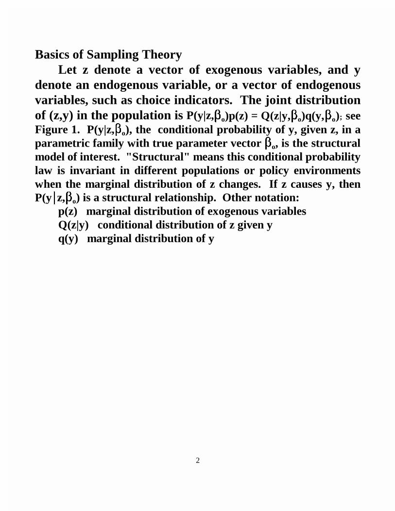
Basics of Sampling TheoryLet z denote a vector of exogenous variables, and y

denote an endogenous variable, or a vector of endogenousvariables, such as choice indicators. The joint distributionof (z,y) in the population is P(y|z,��o)p(z) = Q(z|y,��o)q(y,��o); seeFigure 1. P(y|z,��o), the conditional probability of y, given z, in aparametric family with true parameter vector ��o, is the structuralmodel of interest. "Structural" means this conditional probabilitylaw is invariant in different populations or policy environmentswhen the marginal distribution of z changes. If z causes y, thenP(y z,��o) is a structural relationship. Other notation:

p(z) marginal distribution of exogenous variablesQ(z|y) conditional distribution of z given yq(y) marginal distribution of y

3

Figure 1. Population Probability Model

y1 y2 ... yJ Total

z1 P(y1|z1,��0)p(z1) P(y2|z1,��0)p(z1) P(yJ|z1,��0)p(z1) p(z1)

z2 P(y1|z2,��0)p(z2) P(y2|z2,��0)p(z2) P(yJ|z2,��0)p(z2) p(z2)

:

zK P(y1|zK,��0)p(zK) P(y2|zK,��0)p(zK) P(yJ|zK,��0)p(zK) p(zK)

Total q(y1,��0) q(y2,��0) q(yJ,��0) 1

4

A simple random sample draws independentobservations from the population, each with probabilitylaw P(y|z,��o)��p(z). The kernel of the log likelihood of thissample depends only on the conditional probabilityP(y|z,��), not on the marginal density p(z); thus, maximumlikelihood estimation of the structural parameters ��o doesnot require that the marginal distribution p(z) beparameterized or estimated. ��o influences only how dataare distributed within rows of the table above; and how thedata are distributed across rows provides no additionalinformation on ��o.

5

Stratified Samples. An (exogenously) stratified randomsample samples among rows with probability weightsdifferent from p(z), but within rows the sample isdistributed with the probability law for the population.Just as for a simple random sample, the samplingprobabilities across rows do not enter the kernel of thelikelihood function for ��o, so the exogenously stratifiedrandom sample can be analyzed in exactly the same way asa simple random sample.

The idea of a stratified random sample can beextended to consider what are called endogneous or choice-based sampling protocols. Suppose the data are collectedfrom one or more strata, indexed s = 1,..., S. Each stratumhas a sampling protocol that determines the segment of thepopulation that qualifies for interviewing.

6

Let R(z,y,s) = qualification probability that a populationmember with characteristics (z,y) will qualify for thesubpopulation from which the stratum s subsample will bedrawn. For example, a stratum might correspond to thenorthwest 2x2 subtable in Figure 1, where y is one of thevalues y1 or y2 and z is one of the values z1 or z2. In thiscase, R(z,y,s) equals the sum of the four cell probabilities.Qualification may be related to the sampling frame, whichselects locations (e.g., census tracts, telephone prefixes), toscreening (e.g., terminate interview if respondent is not ahome-owner), or to attrition (e.g., refusals)

Examples:1. Simple random subsample, with R(z,y,s) = 1. 2. Exogenously stratified random subsample, with R(z,y,s) = 1 if z ��

As for a subset As of the universe Z of exogenous vectors, R(z,y,s) = 0otherwise. For example, the set As might define a geographical area. Thiscorresponds to sampling randomly from one or more rows of the table.

7

Exogenous stratified sampling can be generalized tovariable sampling rates by permitting R(z,y,s) to be anyfunction from (z,s) into the unit interval; a protocol forsuch sampling might be, for example, a screening interviewthat qualifies a proportion of the respondents that is afunction of respondent age.

8

3. Endogenously stratified subsample: R(z,y,s) = 1 if y�� Bs, with Bs a subset of the universe of endogenousvectors Y, and R(z,y,s) = 0 otherwise. The set Bs mightidentify a single alternative or set of alternatives amongdiscrete responses, with the sampling frame interceptingsubjects based on their presence in Bs; e.g., buyers whoregister their purchase, recreators at national parks.Alternately, Bs might identify a range of a continuousresponse, such as an income category. Endogenoussampling corresponds to sampling randomly from one ormore columns of the table. A choice-based sample fordiscrete response is the case where each response is adifferent stratum. Then R(z,y,s) = 1(y = s).

9

Endogenous stratified sampling can be generalized toqualification involving both exogenous and endogenousvariables, with Bs defined in general as a subset of Z×Y.For example, in a study of mode choice, a stratum mightqualify bus riders (endogenous) over age 18 (exogenous). Itcan also be generalized to differential sampling rates, witha proportion R(z,y,s) between zero and one qualifying in ascreening interview.

4. Sample selection/attrition, with R(z,y,s) giving theproportion of the population with variables (z,y) whoseavailability qualifies them for stratum s. For example,R(z,y,s) may give the proportion of subjects with variables(z,y) that can be contacted and will agree to be interviewed,or the proportion of subjects meeting an endogenousselection condition, say employment, that qualifies them forobservation of wage (in z) and hours worked (in y).

10

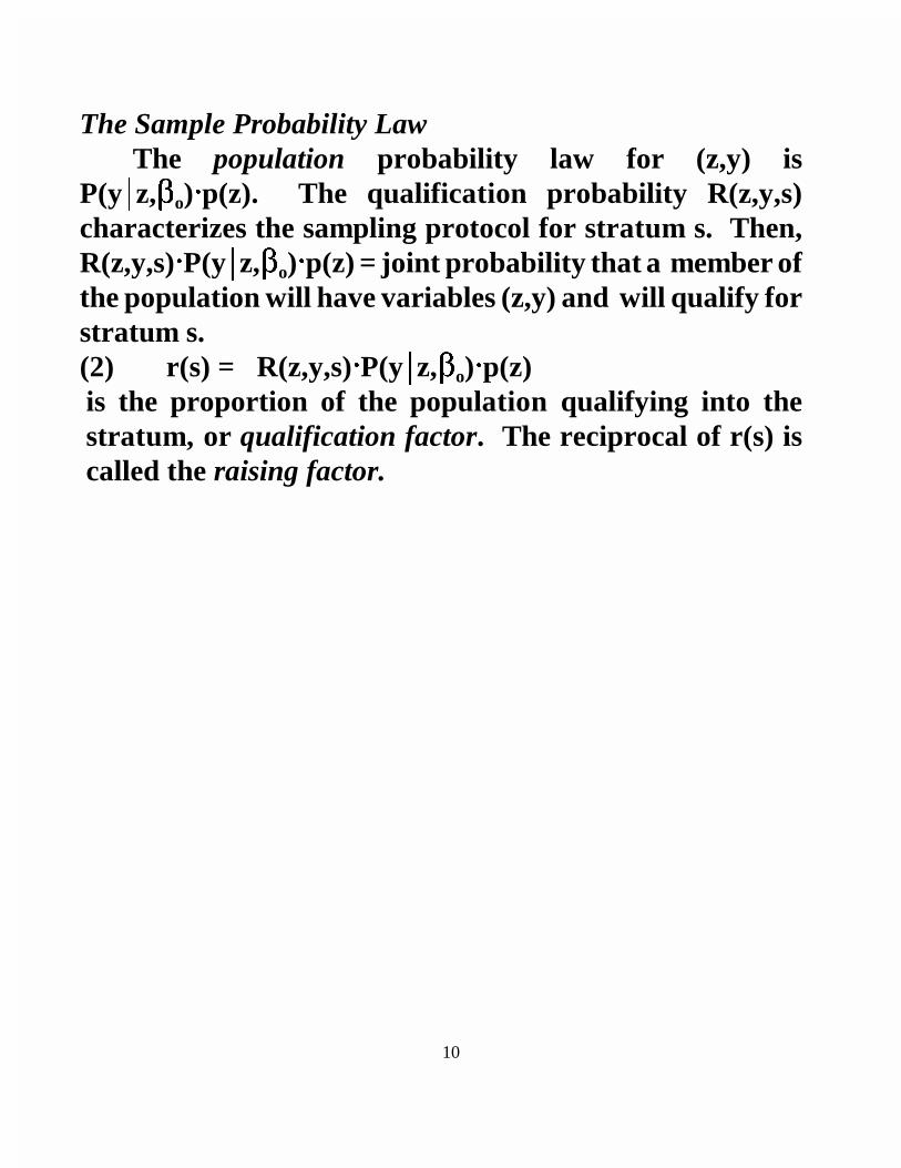
The Sample Probability LawThe population probability law for (z,y) is

P(y z,��o)��p(z). The qualification probability R(z,y,s)characterizes the sampling protocol for stratum s. Then,R(z,y,s)��P(y z,��o)��p(z) = joint probability that a member ofthe population will have variables (z,y) and will qualify forstratum s.(2) r(s) = R(z,y,s)��P(y z,��o)��p(z)

is the proportion of the population qualifying into thestratum, or qualification factor. The reciprocal of r(s) iscalled the raising factor.

11

(3) G(z,y s) = R(z,y,s)��P(y z,��o)��p(z)/r(s),

the conditional distribution G(z,y s) of (z,y) givenqualification, is the sample probability law for stratum s.The probability law G(z,y s) depends on the unknownparameter vector ��, on p(z), and on the qualificationprobability R(z,y,s). In simple cases of stratification,R(z,y,s) is fully specified by the sampling protocol. Thequalification factor r(s) may be known (e.g., stratificationbased on census tracts with known sizes); estimated fromthe survey (e.g.; qualification is determined by a screeninginterview); or estimated from an auxiliary sample. In caseof attrition or selection, R(z,y,s) may be an unknownfunction, or may contain unknown parameters.

12

The precision of the maximum likelihood estimator willdepend on the qualification factor. Suppose a randomsample of size ns is drawn from stratum s, and let N = ��sns

denote total sample size. Let n(z,y s) denote the numberof observations in the stratum s subsample that fall in cell(z,y). Then, the log likelihood for the stratified sample is

(4) L = n(z,y s)��Log G(z,y s).

13

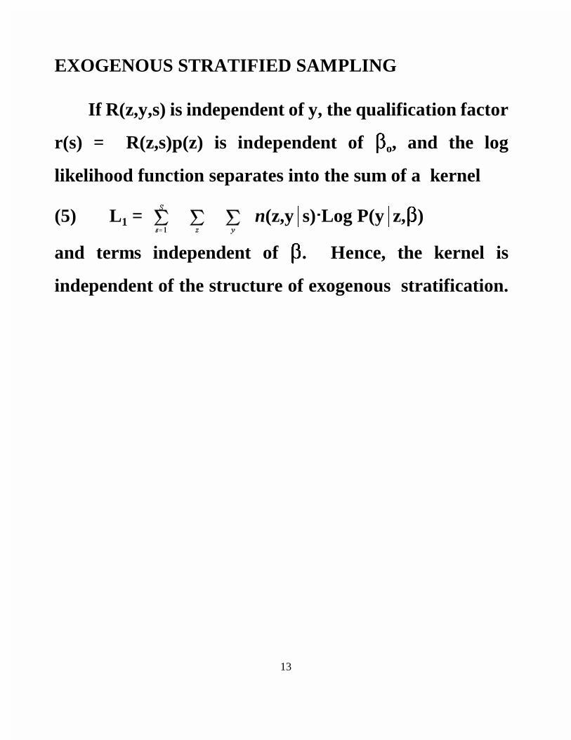
EXOGENOUS STRATIFIED SAMPLING

If R(z,y,s) is independent of y, the qualification factor

r(s) = R(z,s)p(z) is independent of ��o, and the log

likelihood function separates into the sum of a kernel

(5) L1 = n(z,y s)��Log P(y z,��)

and terms independent of ��. Hence, the kernel is

independent of the structure of exogenous stratification.

14

ENDOGENOUS STRATIFICATION

Suppose the qualification probability R(z,y,s) dependson y. Then the qualification factor (2) depends on ��o, andthe log likelihood function (4) has a kernel depending ingeneral not only on ��, but also on the unknown marginaldistribution p(z). Any unknowns in the qualificationprobability also enter the kernel.

There are four possible strategies for estimation underthese conditions:

1. Brute force -- Assume p(z) and, if necessary,R(z,y,s), are in parametric families, and estimate theirparameters jointly with ��. For example, in multivariatediscrete data analysis, an analysis of variancerepresentation absorbs the effects of stratification.

15

2. Weighted Exogenous Sample Maximum Likelihood(WESML) This is a quasi-maximum likelihood approachwhich starts from the likelihood function appropriate to arandom sample, and reweights the data (if possible) toachieve consistency. A familiar form of this approach isthe classical survey research technique of reweighting asample so that it appears to be a simple random sample.

3. Conditional Maximum Likelihood (CML): Thisapproach pools the observations across strata, and thenforms the conditional likelihood of y given z in this pool. This has the effect of conditioning out the unknowndensity p(z).

4. Full Information Maximum Likelihood (FICLE):This approach formally maximizes the likelihood functionin p(z) as a function of the data, the remaining parameters,and a finite vector of auxiliary parameters, and thenconcentrates the likelihood function by substituting inthese formal maximum likelihood estimates for p(z).

16

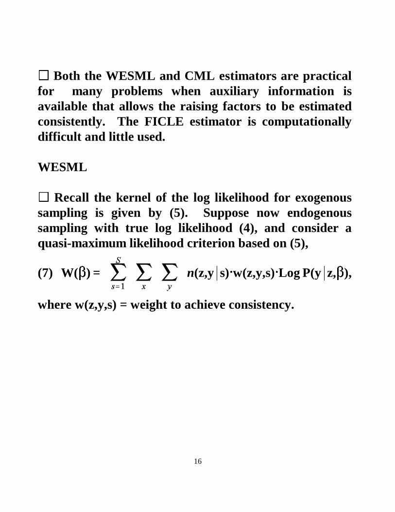
** Both the WESML and CML estimators are practicalfor many problems when auxiliary information isavailable that allows the raising factors to be estimatedconsistently. The FICLE estimator is computationallydifficult and little used.

WESML

** Recall the kernel of the log likelihood for exogenoussampling is given by (5). Suppose now endogenoussampling with true log likelihood (4), and consider aquasi-maximum likelihood criterion based on (5),

(7) W(��) = n(z,y s)��w(z,y,s)��Log P(y z,��),

where w(z,y,s) = weight to achieve consistency.

17

** Suppose r(s) is consistently estimated by f(s), fromgovernment statistics, survey frame data such as theaverage refusal rate, or an auxiliary sample. Consider theweights

(11) w(z,y) = 1/ ;

these are well-defined if the bracketed expressions arepositive and R(z,y,s) contains no unknown parameters. Aclassical application of WESML estimation is to a sample inwhich the strata coincide with the possible configurations ofy, so that R(z,y,s) = 1(y = s). In this case, w(z,y) = N��f(y)/ny,the ratio of the population to the sample frequency. This isthe raising factor encountered in classical survey research.Another application is to enriched samples, where a randomsubsample (s = 1) is enriched with an endogenoussubsamples from one or more configurations of y; e.g., s =y = 2. Then, w(z,1) = N/n1 and w(z,2) = N��f(2)/[n1��f(2) + n2].

18

CMLPool the observations from the different strata.

Then, the data generation process for the pooled sampleis

(15) Pr(z,y) = G(z,y,s)ns/N,

and the conditional probability of y given z from thispool is

(17) Pr(y|z) = .

The CML estimator maximizes the conditionallikelihood of the pooled sample in �� and any unknownsin R(z,y,s). When r(s) is known, or one wishes tocondition on estimates f(s) of r(s) from auxiliarysamples, (17) is used directly. More generally, givenauxiliary sample information on the r(s), these can betreated as parameters and estimated from the jointlikelihood of (17) and the likelihood of the auxiliarysample.

19

For discrete response in which qualification doesnot depend on z, the formula (17) simplifies to

Pr(y z) = ,

where ��y = R(z,y,s)��ns/N��r(s) can be treated as analternative-specific constant. For multinomial logitchoice models, Pr(y z) then reduces to a multinomiallogit formula with added alternative-specific constants.It is possible to estimate this model by the CML methodusing standard random sample computer programs forthis model, obtaining consistent estimates for slopeparameters, and for the sum of log ��y andalternative-specific parameters in the original model.What is critical for this to work is that the MNL modelcontain alternative-specific dummy variablescorresponding to each choice-based stratum.

** For an enriched sample, Pr(1 z) = P(1 z,��o)��n1/N��Dand Pr(2 z) = P(2 z,��o)��[n1/N + n2/N��r(2)]/D, whereD = n1/N + P(2 z,��o)��n2/N.

** Example: Suppose y is a continuous variable, andthe sample consists of a single stratum in which highincome families are over-sampled by screening, so that

20

the qualification probability is R(z,y,1) = �� < 1 for y ��yo and R(z,y,1) = 1 for y > yo. Then Pr(y z) =����P(y z,��o)/D for y �� yo and Pr(y z) = P(y z,��o)/D fory > yo, where D = �� + (1-��)��P(y>yo z,��o).

** Both the WESML and CML estimators arecomputationally practical in a variety of endogenoussampling situations, and have been widely used.

21

Sampling of Alternatives for EstimationConsider a simple or exogenously stratified random

sample and discrete choice data to which one wishes tofit a multinomial logit model. Suppose the choice set isvery large, so that the task of collecting attribute datafor each alternative is burdensome, and estimation ofthe MNL model is difficult. Then, it is possible toreduce the collection and processing burden greatly byworking with samples from the full set of alternatives.There is a cost, which is a loss of statistical efficiency.Suppose Cn is the choice set for subject n, and the MNLprobability model is written

Pin =

where in is the observed choice and Vin = xin.�� is thesystematic utility of alternative i.

Suppose the analyst selects a subset of alternativesAn for this subject which will be used as a basis forestimation; i.e., if in is contained in An, then the subjectis treated as if the choice were actually being madefrom An, and if in is not contained in An, the observationis discarded. In selecting An, the analyst may use the

22

information on which alternative in was chosen, andmay also use information on the variables that enter thedetermination of the Vin. The rule used by the analystfor selecting An is summarized by a probability%%(A in,V's) that subset A of Cn is selected, given theobserved choice in and the observed V's (or, moreprecisely, the observed variables behind the V's).

23

The selection rule is a uniform conditioning rule if forthe selected An, it is the case that %%(An j,V's) is thesame for all j in An. Examples of uniform conditioningrules are (1) select (randomly or purposively) a subsetAn of Cn without taking into account what the observedchoice or the V's are, and keep the observation if andonly if in is contained in the selected An; and (2) givenobserved choice in. select m-1 of the remainingalternatives at random from Cn, without taking intoaccount the V's.

24

An implication of uniform conditioning is that inthe sample containing the pairs (in,An) for which in iscontained in An, the probability of observed response in

conditioned on An is

=

This is just a MNL model that treats choice as if itwere being made from An rather than Cn, so thatmaximum likelihood estimation of this model for thesample of (in,An) with in �� An estimates the sameparameters as does maximum likelihood estimation ondata from the full choice set. Then, this sampling ofalternatives cuts down data collection time (foralternatives not in An) and computation size and time,but still gives consistent estimates of parameters forthe original problem.

25

BIVARIATE SELECTION MODEL

(29) y* = x�� + JJ ,w* = z�� + )�)� ,

x, z vectors of exogenous variables, not necessarilyall distinct,

��, �� parameter vectors, not necessarily all distinct, )) a positive parameter. y* latent net desirability of work, w* latent log potential wage.

NORMAL MODEL

(30) ~ N ,

correlation ''.

26

Observation rule

"Observe y = 1 and w = w* if y* > 0; observe y = -1 and do notobserve w when y* �� 0".

The event of working (y = 1) or not working (y = 0) isobserved, but net desirability is not, and the wage is observedonly if the individual works (y* > 0).

For some purposes, code the discrete response as s = (y+1)/2;then s = 1 for workers, s = 0 for non-workers.

The event of working is given by a probit model.

00 is the standard univariate cumulative normal.

The probability of working is

P(y=1 x) = P(JJ > -x��) = 00(x��),

The probability of not working is

P(y=-1 x) = P(JJ �� -x��) = 00(-x��).

Compactly,

P(y x) = 00(yx��).

27

In the bivariate normal, the conditional density of onecomponent given the other is univariate normal,

JJ �� ~ N('�'�,1-''2) =

and

�� JJ ~ N('J'J,1-''2) = .

28

The joint density: marginal times conditional,

(JJ,��) ~ 11(��)��

= 11(JJ)�� .

The density of (y*,w*)(31) f(y*,w*)

= 11( )�� ��11

= 11(y*-x��)�� ��11 .

Log likelihood of an observation, l(��,��,)),'').

In the case of a non-worker (y = -1 and w = NA), the density(31) is integrated over y* < 0 and all w*. Using the second formin (31), this gives probability 00(-x��).

29

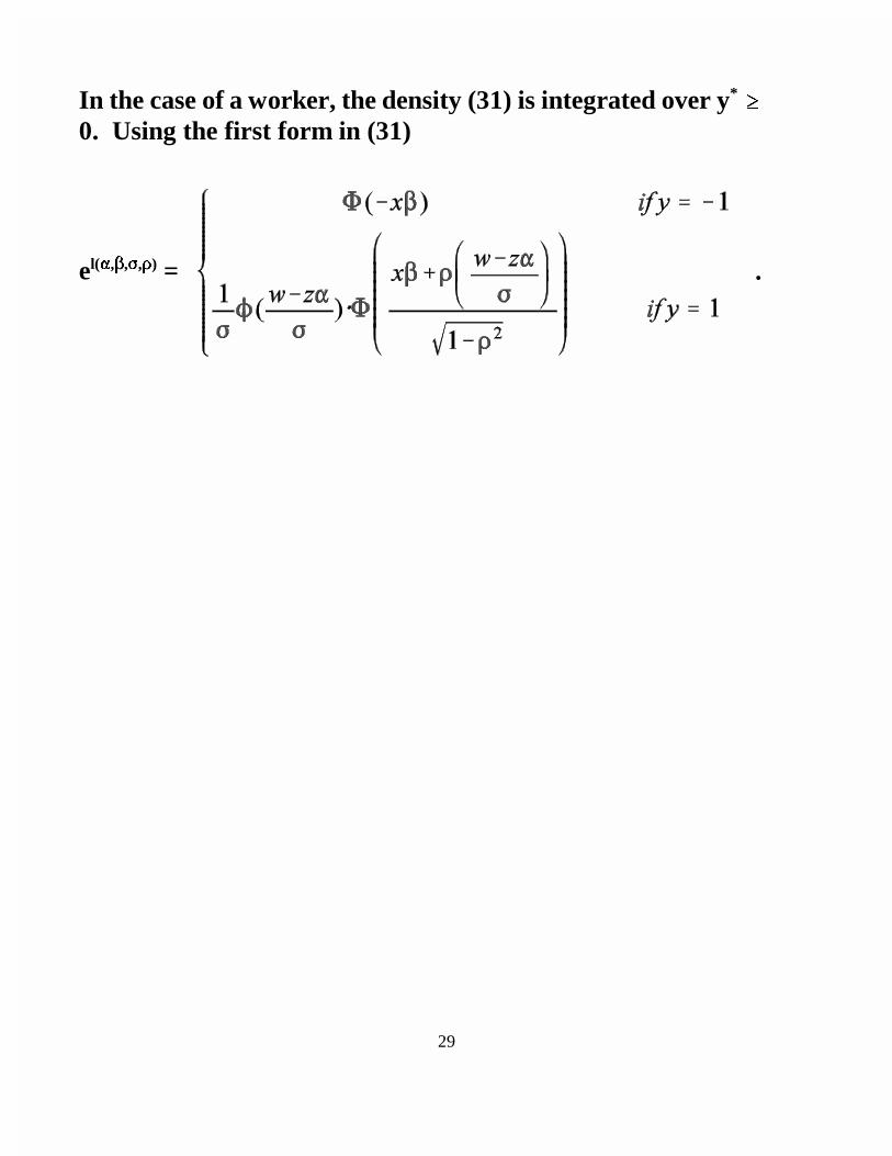
In the case of a worker, the density (31) is integrated over y* ��0. Using the first form in (31)

el(��,��,)),'') = .

30

The log likelihood can be rewritten as the sum of the marginal loglikelihood of the discrete variable y and the conditional loglikelihood of w given that it is observed, l(��,��,)),'') = l1(��,��) +l2(��,��,)),''), with the marginal component,

(33) l1(��) = log 00(yx��) ,

and the conditional component (that appears only when y = 1),

(34) l2(�,�,),') = -log ) + log 1( ) + log

0 - log 0(x�) .

One could estimate this model by maximizing the sample sum of the fulllikelihood function l, by maximizing the sample sum of either themarginal or the conditional component, or by maximizing thesecomponents in sequence.

Note that asymptotically efficient estimation requires maximizing thefull likelihood, and that not all the parameters are identified in eachcomponent; e.g., only � is identified from the marginal component.

31

Nevertheless, there may be computational advantages to working withthe marginal or conditional likelihood. Maximization of l1 is aconventional binomial probit problem. Maximization of l2 could bedone either jointly in all the parameters �, �, ', ); or alternately in �,', ), with the estimate of � from a first-step binomial probit substitutedin and treated as fixed.

32

When ' = 0, the case of "exogenous" selection in which there is nocorrelation between the random variables determining selection into theobserved population and the level of the observation, l2 reduces to thelog likelihood for a regression with normal disturbances. When ' g 0,selection matters and regressing of w on z will not give consistentestimates of � and ).

33

An alternative to maximum likelihood estimation is a GMM procedurebased on the moments of w. Using the property that the conditionalexpectation of � given y = 1 equals the conditional expectation of �given J, integrated over the conditional density of J given y = 1, plus theproperty of the normal that d1(J)/dJ = -J�1(J), one has

(35) E{w z,y=1} = z� + )E{� y=1} = z� + ) E{� J}1(J)dJ/0(x�)

= z� + )' J1(J)dJ/0(x�)

= z� + )'1(x�)/0(x�) � z� + �M(x�),

where � = )' and M(c) = 1(c)/0(c) is called the inverse Mill's ratio.

34

Further, E(�2 J) = Var(� J) + {E(� J)}2

= 1 - '2 + '2J

2,

J

21(J)dJ = - J11(J)dJ

= -c1(c) + 1(J)dJ

= -c1(c) + 0(c),

(36) E{(w-z�)2 z,y=1} = )2E{�2 y=1}

= )2 E{�2 J}1(J)dJ/0(x�)

= )2 {1 - '2 + '2J

2}1(J)dJ/0(x�)

= )2{1 - '2 + '2 - '2x�1(x�)/0(x�)} = )2{1 - '2x�1(x�)/0(x�)} = )2{1 - '2x��M(x�)}.

Then,

35

(37) E =

E{(w-z�)2 z,y=1} - [E{w-z� z,y=1}]2

= )2{1 - '2x�1(x�)/0(x�) - '21(x�)2/0(x�)2}

= )2{1 - '2M(x�)[x� + M(x�)}.

36

A GMM estimator for this problem can be obtained by applying NLLS,

for the observations with y = 1, to the equation

(38) w = z� + )'M(x�) + �,

where � is a disturbance that satisfies E{� y=1} = 0. This ignores the

heteroskedasticity of �, but it is nevertheless consistent. This regression

estimates only the product � � )'.

37

Consistent estimates of ) and ' could be obtained in a second step:

(39) V{� x,z,y=1}

= )2{1 - '2M(x�)[x� + M(x�)]},

Estimate )2 by regressing the square of the estimated residual, �e2,

(40) �e2 = a + b{M(x�e)[x�e + M(x�e)]} + !

provide consistent estimates of )2 and )2'

2, respectively.

38

There is a two-step estimation procedure, due to Heckman, that requires

only standard computer software, and is widely used:

[1] Estimate the binomial probit model,

(42) P(y x,�) = 0(yx�) ,

by maximum likelihood.

[2] Estimate the linear regression model,

(43) w = z� + �M(x�e) + �,

where � = )' and the inverse Mill's ratio M is evaluated at the

parameters estimated from the first stage.

To estimate ) and ', and increase efficiency, one can do an

additional step,

[3] Estimate )2 using the procedure described in (40), with

estimates �e from the second step and �e from the first step.

39

One limitation of the bivariate normal model is most easily

seen by examining the regression (43). Consistent estimation of the

parameters � in this model requires that the term M(x�|) be

estimated consistently. This in turn requires the assumption of

normality, leading to the first-step probit model, to be exactly right.

Were it not for this restriction, estimation of � in (43) would be

consistent under the much more relaxed requirements for

consistency of OLS estimators. To investigate this issue further,

consider the bivariate selection model (29) with the following more

general distributional assumptions: (i) J has a density f(J) and

associated CDF F(J); and (ii) � has E(� J) = 'J and a second

moment E(�2 J) = 1 - '2 that is independent of J. Define the

truncated moments

J(x�) = E(J J>-x�)

= Jf(J)dJ/[1 - F(-x�)]

and

K(x�) = E(1 - J2 J>-x�)

40

= [1 - J2]f(J)dJ/[1 - F(-x�)] .

Then, given the assumptions (i) and (ii),

E(w z,y=1) = z� + )'E(J J>-x�)

= z� + )'J(x�),

E((w - E(w z,y=1))2 z,y=1)

= )2{1 - '2[K(x�) + J(x�)2]}.

Thus, even if the disturbances in the latent variable model were notnormal, it would nevertheless be possible to write down aregression with an added term to correct for self-selection thatcould be applied to observations where y = 1:

(45) w = z� + )E{� x�+J>0} + � = z� + )'J(x�) + �,

where � is a disturbance that has mean zero and the heteroskedasticvariance

E(�2 z,y=1)) = )2{1 - '2[K(x�) + J(x�)2]}.

Now suppose one runs the regression (37) with an inverse Mill'sratio term to correct for self-selection, when in fact the disturbancesare not normal and (44) is the correct specification. What biasresults? The answer is that the closer M(x�) is to J(x�), the less

41

the bias. Specifically, when (44) is the correct model, regressingw on z and M(x�) amounts to estimating the misspecified model

w = z� + �M(x�) + {� + �[J(x�) - M(x�)]} .

42

The bias in NLLS is given by

= �

this bias is small if � = )' is small or the covariance of J - M withz and M is small.