Embed Size (px)
Citation preview

LAPPEENRANTA UNIVERSITY OF TECHNOLOGY LUT School of Engineering and Science Master´s Degree Programme in Industrial Engineering
Sampo Järvinen Profitability potential of high value added cellulosic raw materials in China Examiner/Supervisor: Professor Timo Kärri Examiner: University lecturer Leena Tynninen
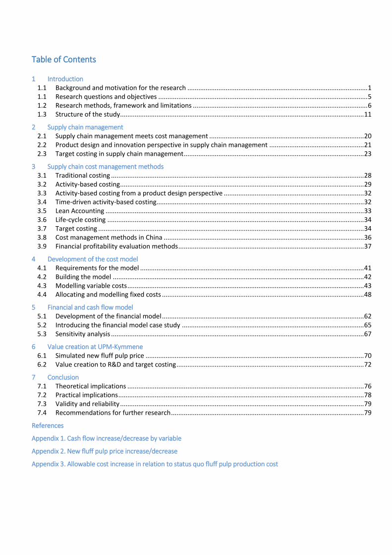
Table of Contents
1 Introduction 1.1 Background and motivation for the research ................................................................................................... 1 1.1 Research questions and objectives ................................................................................................................... 5 1.2 Research methods, framework and limitations ................................................................................................ 6 1.3 Structure of the study ...................................................................................................................................... 11
2 Supply chain management 2.1 Supply chain management meets cost management ..................................................................................... 20 2.2 Product design and innovation perspective in supply chain management .................................................... 21 2.3 Target costing in supply chain management ................................................................................................... 23
3 Supply chain cost management methods 3.1 Traditional costing ........................................................................................................................................... 28 3.2 Activity-based costing ...................................................................................................................................... 29 3.3 Activity-based costing from a product design perspective ............................................................................. 32 3.4 Time-driven activity-based costing .................................................................................................................. 32 3.5 Lean Accounting .............................................................................................................................................. 33 3.6 Life-cycle costing ............................................................................................................................................. 34 3.7 Target costing .................................................................................................................................................. 34 3.8 Cost management methods in China .............................................................................................................. 36 3.9 Financial profitability evaluation methods ...................................................................................................... 37
4 Development of the cost model 4.1 Requirements for the model ........................................................................................................................... 41 4.2 Building the model .......................................................................................................................................... 42 4.3 Modelling variable costs .................................................................................................................................. 43 4.4 Allocating and modelling fixed costs ............................................................................................................... 48
5 Financial and cash flow model 5.1 Development of the financial model ............................................................................................................... 62 5.2 Introducing the financial model case study .................................................................................................... 65 5.3 Sensitivity analysis ........................................................................................................................................... 67
6 Value creation at UPM-Kymmene 6.1 Simulated new fluff pulp price ........................................................................................................................ 70 6.2 Value creation to R&D and target costing ....................................................................................................... 72
7 Conclusion 7.1 Theoretical implications .................................................................................................................................. 76 7.2 Practical implications ....................................................................................................................................... 78 7.3 Validity and reliability ...................................................................................................................................... 79 7.4 Recommendations for further research .......................................................................................................... 79
References
Appendix 1. Cash flow increase/decrease by variable
Appendix 2. New fluff pulp price increase/decrease
Appendix 3. Allowable cost increase in relation to status quo fluff pulp production cost

ABSTRACT Author: Sampo Järvinen Title: Profitability potential of high value added cellulosic raw materials in China Year: 2019 Place: Lappeenranta Master’s thesis. Lappeenranta University of Technology, LUT School of Business and Management 80 pages, 28 figures, 16 tables, 18 equations and 3 appendices Examiner: Professor Timo Kärri
Supervisors: Dr. Matti Ristolainen, UPM Pulp Business, Research and Innovation
Dr. Harri Kosonen, UPM Pulp Business, Research and Innovation Keywords: Traditional costing, activity-based costing, time driven activity-based costing,
target costing, target pricing, supply chain management, supply chain innovation, financial modelling, product development, fluff pulp
The objective of this Master’s thesis is to determine what would be the target cost and target price for several new kinds of fluff pulps developed and produced if innovated based on the market conditions in China. The aim is to find the most value creating, profitable and feasible innovation focus areas on new fibre development for fluff pulp and ultimately steer the research and development actions.
This study has been executed using decision-making methodological strategy research methodology combined with Balanced approach research method. The research is an innovative and practice oriented case study, consisting of the development of a financial simulation model. The study includes informal interview with supply chain management professionals in China and participant observations such as manufacturing site visitations. Theoretical part of the thesis is based on literature review.
In this thesis, three models were created, a cost model, financial model and cash flow model. In the cost model three alternative costing methods were used and compared: traditional costing, activity-based costing and time driven activity-based costing. In the financial model financial metrics between status quo and alternative operating setting were compared. In the cash flow model, target costing was implemented to quantify what brings most value to the customer and what would be the new price for different fluff pulp development areas.
Based on the results, pulp value chain’s R&D sector should focus on helping customer increase selling price. In addition, latex binder addition, fixed costs and web’s basis weight show clear improvement potential. Hammermill energy consumption and drying energy which were assumed to play an important role, did not in the end show as big of an impact as the ones previously listed. These results can be generalised to be valid not only in China but also in globally by keeping in mind there might be slight variations in different cost group’s significances.

TIIVISTELMÄ Tekijä: Sampo Järvinen Työn nimi: Korkean lisäarvon sellumateriaalien kannattavuuspotenttiaali Kiinassa Vuosi: 2019 Paikka: Lappeenranta Diplomityö. Lappeenrannan teknillinen yliopisto, tuotantotalous. 80 sivua, 28 kuvaa, 16 taulukkoa, 18 yhtälöä ja 3 liitettä Tarkastaja: Professori Timo Kärri
Ohjaajat: Dr. Matti Ristolainen, UPM Pulp Business, Research and Innovation
Dr. Harri Kosonen, UPM Pulp Business, Research and Innovation Hakusanat: Perinteinen kustannuslaskenta, toimintoperusteinen kustannuslaskenta, aikaohjattu toimintoperusteinen kustannuslaskenta, tavoite kustannus, tavoite hinta, toimitusketjun johtaminen, taloudellinen mallintaminen, tuotekehitys, fluff-sellu Tämän diplomityön tavoitteena on määrittää tavoitekustannus ja –hinta erityyppisille uusille fluffi sellulaaduille Kiinan markkinoille. Tavoitteena on löytää eniten asiakkaille arvoa luovat, tuottoisat ja toteutettavissa olevat fluffikuitujen innovaatioalueet ja lopulta ohjata tutkimus- ja kehitystoimia näitä kohti.
Tämä tutkimus on toteutettu päätöksentekomenetelmästrategian tutkimusmetodologialla yhdistettynä tasapainotetun lähestymistavan tutkimusmenetelmään. Tutkimus on innovatiivis-käytännänläheinen tapaustutkimus sisältäen taloudellisen simulaatiomallin. Työssä on hyödynnetty haastatteluja johtavien kiinalaisten toimitusketjun johtamisen ammattilaisien kanssa sekä havainnointia tuotantolaitoksilla. Teoreettinen osuus työstä perustuu kirjallisuuskatsaukseen.
Työssä luotiin kolme eri mallia: kustannuslaskenta-, tilinpäätös- ja kassavirtamalli. Kustannuslaskentamallissa sovellettiin kolmea eri kustannuslaskentamenetelmää: perinteistä, toimintoperusteista ja aikaohjattua toimintoperusteista kustannuslaskentaa (engl. time-driven activity based costing). Tilinpäätösmallissa status quo ja simuloidun tuotannon väliä vertailtiin taloudellisilla mittareilla. Kassavirtamallissa, tavoite kustannus-metodia –metodia sovellettiin kvantifioimaan mikä luo asiakkaalle eniten arvoa ja mikä voisi olla uuden fluffikuidun myyntihinta eri kehitysalueilla.
Tulosten perusteella selluarvoketjun tutkimus-ja kehitysyksikön tulisi keskittyä asiakkaan tuotteen myyntihinnan korottamiskeinoihin. Lisäksi, lateksisideaineen vähennys, kiinteiden kustannusten lasku ja neliöpainon pienentäminen ovat potentiaalisia kehityskohteita. Vasaramyllyn energiakulutuksen ja kuivausenergian pienentäminen eivät olleet yhtä merkittäviä kuin tutkimuksen alussa oli ajateltu. Tulokset voidaan yleistää pitävän paikkansa Kiinan lisäksi myös globaalisti ottamalla huomioon pienet vaihtelut kustannusrakenteessa eri maiden välillä.

Acknowledgements This thesis was conducted at Lappeenranta University of Technology in the School of Engineering
Science and the Cost Management major.
I would like to thank Professor Timo Kärri for providing supervision and guidance for tis thesis. I also
want to express my gratitude for my instructor Leena Tynninen who gave me valuable feedback and
help. In addition, from UPM’s side I thank Dr. Matti Ristolainen and Dr. Harri Kosonen for their
guidance and working premises regarding this thesis. Without them, this such a great journey would
not have been possible.
Additionally, there are many UPMers in China that have supported me throughout my half a year
stay in Shanghai. Specials thanks goes to Wenqing Wang, Roberto Mirande and Wenxia Wu for
providing their contacts, helping hand and feedback. Without the APAC’s Technical customer service
team and Sales team, this thesis would not have gotten its depth from real customer cases.
Finally, heartfelt thanks for my family and friends for the never-ending support.

TABLE OF FIGURES AND TABLES
Figures Figure 1. Fluff pulp consumption and their growth rates ................................................................................. 2 Figure 2. Fluff pulp end use application areas by end-use, 2015 ...................................................................... 3 Figure 3. Global fluff pulp consumption by raw material.................................................................................. 3 Figure 4. Fluff pulp production rates by region in 2015 .................................................................................... 4 Figure 5. Raw materials typically used in nonwovens ....................................................................................... 5 Figure 6. The Balanced Approach Model .......................................................................................................... 8 Figure 7. Research Design in relation to other business and management research methods. ..................... 10 Figure 8. Research focus in the Product-Relationship-Matrix of Supply Chain Management ........................ 11 Figure 9. Evolution of supply chain management from 1960 to 2000 and beyond ........................................ 15 Figure 10. The divergence and connection point of supply chain management and supply chain cost
management .................................................................................................................................. 17 Figure 11. Illustrative total cost in the supply channel ................................................................................... 19 Figure 12. Supply chain material flow in an optimal case ............................................................................... 21 Figure 13. Illustration of three costing methods: traditional costing, activity-based costing and time-driven
activity-based costing .................................................................................................................... 32 Figure 14. The basic principle of target cost determination ........................................................................... 35 Figure 15. Target costing process .................................................................................................................... 36 Figure 16. Value chain partner’s main operations in end-product manufacturing......................................... 43 Figure 17. Hammermill and former. Screenshot of the model’s hammermill and former input variables .... 44 Figure 18. Latex binder addition and drying section ....................................................................................... 47 Figure 19. Total production, and summary of raw material usages and costs ............................................... 48 Figure 20. Proportion of the total overhead per ton by product with different costing systems .................. 58 Figure 21. Cost breakdown of products to variable and fixed cost by costing system ................................... 59 Figure 22. Net margin by product with different costing systems .................................................................. 60 Figure 23. Illustrative example of the financial model .................................................................................... 62 Figure 24. Illustrative example of the cash flow model .................................................................................. 63 Figure 25. Illustration of model's working capital calculation ......................................................................... 64 Figure 26. Cumulative marginal discounted cash flow increase ..................................................................... 67 Figure 27. Sensitivity analysis: Cumulative net cash flow increase/decrease ................................................. 69 Figure 28. Sensitivity analysis: New fluff pulp price increase/decrease ......................................................... 71 Figure 29. Allowable increase in costs in relation to fluff pulp production cost ............................................. 73 Figure 30. Variations of different costing methods to perceived net margin ................................................. 77

Tables Table 1. Preferred Research Methods in Supply Chain Management ............................................................. 9 Table 2. Structure of the study ........................................................................................................................ 12 Table 3. Typical cost structure of a 600 kt/a softwood chemical pulp mill at full production ........................ 19 Table 4. Evolution of cost measures ................................................................................................................ 27 Table 5. Advantages and disadvantages of activity-based costing ................................................................. 31 Table 6. Different approaches summary for information generated from each accounting system ............. 34 Table 7. List of model’s variables in hammermill and former ......................................................................... 45 Table 8. All fixed costs ..................................................................................................................................... 50 Table 9. Costing from customer’s point of view by using traditional costing ................................................. 51 Table 10. Defining overhead application rates ................................................................................................ 53 Table 11. Costing from customer’s point of view by using Activity-based costing ......................................... 54 Table 12. Product cost by using time driven activity-based costing ............................................................... 55 Table 13. Capacity cost rates ........................................................................................................................... 56 Table 14. Costing from customer’s point of view by using Time driven activity-based costing ..................... 57 Table 15. Fixed cost allocation increase/decrease compared to traditional costing ...................................... 60 Table 16. Fluff pulp grades used before and after the modifications ............................................................. 66

Equations
(1) Net Present Value ............................................................................................................................. 38 (2) Modified Internal Rate of Return ..................................................................................................... 38 (3) Economic Value Addition (Version 1) ............................................................................................... 39 (4) Economic Value Addition (Version 2) ............................................................................................... 39 (5) Return on Capital Employed ............................................................................................................. 39 (6) Weighted Average Cost of Capital .................................................................................................... 40 (7) Capacity Cost Rate ............................................................................................................................ 54 (8) Account Payables Cycle Time ........................................................................................................... 63 (9) Account Receivables Cycle Time ....................................................................................................... 63 (10) Production Process Cycle Time ......................................................................................................... 63 (11) Raw Material Cycle Time .................................................................................................................. 64 (12) Work in Progress Cycle Time ............................................................................................................ 64 (13) Finished Goods Cycle Time ............................................................................................................... 64 (14) Fixed Cost Cycle Time ....................................................................................................................... 64 (15) Marginal Cash Flow ........................................................................................................................... 66 (16) Discounted Marginal Cash Flow ....................................................................................................... 67 (17) New Fluff Pulp Price .......................................................................................................................... 70 (18) Target Cost ........................................................................................................................................ 72

ABBREVIATIONS ABC – Activity based costing ADt – Air-dried ton CPA – Consumer profitability analysis EBIT – Earnings before interest and taxes EBITDA – Earnings before interest, taxes, depreciation and amortization ETLA – Research Institute of Finnish Economy EVA – Economic value added FMCG – Fast-moving consumer goods GAAP – Generally accepted accounting principles GDP – Gross domestic product GNP – Gross national product IRR – Internal rate of return LCC – Life cycle cost MIRR – Modified internal rate of return NOPAT – Net operating profit after taxes NPV – Net present value ROA – Return on assets ROCE – Return on capital employed ROS – Return on sales SCM – Supply chain management SCCM – Supply chain cost management TDABC – Time driven activity-based costing WACC – Weighted average cost of capital WC – Working capital

1
1 Introduction
1.1 Background and motivation for the research
Recent study conducted by The Research Institute of Finnish Economy (ETLA) shows
that ten most significant companies in Finland calculated by economic value added
contribute 7.6 % of Finland’s GDP. The productivity and the growth rates in these
companies have substantially outperformed the computational average. In addition,
these companies generate notable multiplicative effects to the economy. UPM-
Kymmene Oyj, the company for which this thesis is made is, according to the report
the most significant company for the Finnish economy in terms of the GPD, generating
all together 4084 million euros (1507 by themselves in Finland and 2577 by
multiplicative effects) when the whole value chain is considered. This rises UPM’s
share of the GDP to 2.0 %. (Ali-Yrkko, et al., 2016)
The top companies, UPM-Kymmene included are intertwined with other companies
through their value chains. The positive development of one company ripples on
through its value chain, and the effects are spread to other companies. This makes it
clear that during the decision-making processes on research and development
activities, the whole value chain cost reduction potential, value addition and overall
profitability needs to be taken into account. This is true in existing markets but also in
new market exploration. In order to create a true impact in the value chain by research
and development actions, a true understanding of the value chain is needed. Only the
value creating activities makes sure the feasibility. One of the evaluation method is
financial benefit.
While the concept of supply chain focuses on operations and logistics, in other words
material flows (Tan, 2001), the term “value chain” extends the focus also to
information and cash flows. Information and cash flows have been considered as part
of the supply chain as well in previous literature (Hofmann & Kotzab, 2010), but played
a smaller role compared to logistics. To emphasize the importance of additional value
creation and customer orientation in innovation departments’ key objectives, in this
research the term value chain is selected instead of supply chain. Furthermore, in this
research, value chain management cuts across several disciplines such as operations
management, strategic management and product innovation management, so the
use of (financial) value chain is well-justified.

2
World market pulp demand in 2015 was 63.6 million tonnes, which is 38 % of total
wood pulp consumption. From this, fluff pulp accounts about 10 % and is expected to
grow at a rate of 2.7 % a year. Produced using typically coarse, long-fibre softwoods,
fluff pulp historically has been a specialty pulp grade with higher prices and margins
than the more common papermaking pulp grades. It is one of the most sustainable
raw materials on earth for hygiene and nonwoven products, based on tree species
grown with no or little irrigation, no pesticides on land with no value for food production.
Breaking down the fluff pulp consumption into regions, we can see that Asia is already
the biggest market with a share of almost 40 % of the world’s total fluff pulp
consumption (Figure 1). From Asia’s figure China accounts roughly 30 %. China by
itself accounts for 12 % of the global fluff pulp consumption and keeps on growing the
second fastest after India. Saying that, China is and will be a major market for fluff
pulp and in the future.
Figure 1. Fluff pulp consumption (inner circle) and their growth rates (inside brackets) (RISI, 2016)
From the Asia’s fluff pulp consumption 7.3 % of the sales is nonwovens, which is
interesting market because generally speaking Scandinavian softwood could be the
most suitable to the nonwoven end-uses. In these applications runnability, good
formation, low binder consumption, low shredding energy, even web, opacity and
surface smoothness are valued.

3
Figure 2. Fluff pulp end use application areas by end-use, 2015 (Smithers and Pira, 2015a)
However, the Scandinavian fluff pulp’s advantages should be brought out clearer and
further increase its competitiveness by focused R&D actions as its market share is
currently only 5.2 % of the total fluff pulp’s fibre consumption (Figure 3).
Figure 3. Global fluff pulp consumption by raw material (Smithers and Pira, 2015a)
The competitive landscape for fluff pulp is dominated by large pulp and paper
companies located in North America (Figure 4). Currently, only 7.0 % of the
production is in Western Europe. This is mainly due to the presence of the most
optimal wood species for fluff pulp being located there such as Northern America
Southern pine, Loblolly and Slash. The four largest fluff pulp producers account for
about 80 % of all fluff pulp production in 2015. However, this might change because

4
optimal fibre in the future might be Scandinavian pine and/or spruce due to its
characteristics and various treatment alternatives it has that allows fibre modifications.
Figure 4. Fluff pulp production rates by region in 2015 (Smithers and Pira, 2015a)
As can be seen in the Figure 5 nonwovens pose not only a market potential but also
a huge environmental benefit in terms of replacing fossil-based synthetic materials,
which account currently 82.6 % of the total raw material consumption. Wood pulp,
which is mainly fluff pulp, accounts only 6.9 %. For example, wet wipes are one of the
several major microplastics sources and the biggest reason for costly sewer systems
fatbergs. This could be solved by using wood pulp as a raw material for them instead
of non-biodegradable synthetic materials. This can be done by strengthening the
properties and the overall value chain’s cost competitiveness.

5
Figure 5. Raw materials typically used in nonwovens (Smithers and Pira, 2015b)
1.1 Research questions and objectives
The objective is to determine what would be the target cost and target price for several
new kinds of fluff pulp developed and produced if innovated based on the market
conditions in China. Research aim is to find the most profitable and feasible innovation
focus areas on new fibre development for fluff pulp. The value should be monetarised
both for the fluff pulp producer but also for the customer that would ultimately steer
the research and development actions. Therefore, the research questions can be
divided into one main research question that has three sub-questions.
Main research question:
How Cost Management methods and financial modelling can be utilized to
support R&D function in novel fibre development for a customer in fluff pulp
value chain?
The main research question can be divided into three sub-questions:
Which of the Cost Management methods is most applicable for creating a
model that quantifies the current cost structure of a customer in Mainland
China? How the cost results differ between different approaches?
In which way the model needs to be developed to obtain increased
customers’ value of new pulp grade and new fibre properties? What matters
to the most for a customer and what is the best financial measure to
demonstrate the benefits?
What is the new selling price and allowable additional costs of a potential
new type of fibre sold to a customer in Mainland China?

6
1.2 Research methods, framework and limitations
The research paradigms in industrial management can be divided into five categories:
formal conceptual research strategy, nomothetic strategy, action-oriented strategy,
constructive strategy and decision-making methodological strategy (Olkkonen, 1993).
Usefulness of these paradigms can be estimated by comparing their ability to produce
suitable results for the research problem at hand. The formal conceptual strategy is
used for theory building as definitions exist at the abstract level and do not contain
measurable attributes (Wacker, 2004). Nomothetic strategy is a quantitative approach
where the aim is to make objective observation of the test subjects and to create
general symmetrical rules (Chelpa, 2005). In the action-oriented strategy, the
researcher is an active observer in the research case and makes conclusions and
future recommendations according to the experience analysis. Constructive strategy
focuses on problem-solving by innovating and developing completely new models or
mathematical programmes for specific cases in organisations (Kasanen, et al., 1993).
The fifth research approach, the decision-making strategy, produces solutions for
explicit problems on a more general level.
From the five paradigms, both the constructive strategy and decision-making
methodological strategy would be suitable for this research; however, the latter is the
most suitable and chosen as it delivers practical information for decision-makers and
works well on cost modelling methods that have already been proved to work well. In
this case, forestry sector and particularly in pulp and paper industry, activity-based
costing is already in use and proved to work equally well or better as traditional costing
(Fogelholm, 1993; Korpunen, 2015). In the decision-making methodology, the
problem is firstly specified, then reconstructed into mathematical form and next tested
with case studies (Olkkonen, 1993). In the final step, the mathematical forms and
case study results are evaluated and further suggestions for developing the decision-
making tool are made. This approach is strongly quantitative. However, decision-
making methodology is often considered to require access to a large amount of data
from management information systems, which is typically not possible or the data is
inconsistent, incomplete, in accurate or missing.
In addition, when choosing a research strategy, there are always trade-offs in control,
realism and generalizability. According to (Golicic, et al., 2005), Quantitative research
methods (deductive) optimize control and generalizability (external validity), while
qualitative research methods (inductive) maximizes realism (internal validity). It is
agreed that supply chain management researchers are biased in to the positivist
7
paradigm and therefore past researches that are considered to be valid are mostly
quantitative ones. However, business environment in which supply chain cost
management and companies’ research and development stands are becoming
increasingly complex and less compliant to using just one type of research approach.
Therefore, Golicic et al. (2005) recommends researchers to use balanced approach
where qualitative methods are included “in order to accurately describe, truly
understand and begin to explain contemporary businesses’ phenomena”. This means
qualitative and quantitative research approaches are not substitutes, rather they
observe different aspects (McCracken, 1988). Qualitative research methods are used
for example by bringing in an actual case study of a customer’s operations. In practice
in this research this means a financial model with what the operations can be
simulated by basic parameters. Golicic et al. (2005) describes the importance of this
step by stating “research studies need to utilize qualitative methods in addition to
quantitative methods” to gain relevance in supply chain academics research.
Combining decision-making methodological and balanced research method is well
justified as against of general apprehension the utilization rate of qualitative methods
has been low in the past (Table 1). Especially in North American journals primarily
normative (theoretical models and literature reviews) and quantitative
(simulation/modelling and surveys) researches can be found. Halldorsson & Larsson
(2004) examined supply chain management articles from 1997 through 2004 in
Journal Of Business Logistics (JBL), International Journal of Physical Distribution and
Logistics Management (IJPDLM) and the International Journal of Logistics
Management (IJLM) and found out that only 8 out of 71 employed qualitative methods.
This has been extended to German journals and affirmed the same phenomena and
that only 7% of the articles were based on case studies. The research was
categorised to consist also qualitative research methods if, for example brief
interviews were held prior to survey but the whole methodologies were not described
and still qualitative research had low incidence. It should be kept in mind that research
in Europe relies more on qualitative methods than in North America (Golicic, et al.,
2005, p. 18) but still the situation is rarely much better in most European Universities.
These findings clearly indicate that logistics is dominated by quantitative research and
that more qualitative research is needed and therefore Balanced Research Method is
applied (Figure 6).

8
Figure 6. The Balanced Approach Model (adapted from (Golicic, et al., 2005) & (Woodruff , 2003)
Balanced Approach research method is introduced to this research to bring more
qualitative approach to the quantitative theory-based modelling. The Balanced
Approach Model is usually taken in the use if the business phenomenon of interest is
quite new, dynamic and complex but also if relevant variables are not easily identified
and the context of the study makes extant theories unavailable. In addition,
quantitative approach by itself is not enough to describe the overall phenomenon
behind profitability and customer demands due to the problem’s multiplicity. For these
reasons, the research also needs a qualitative approach in order to build a clearer
picture and ensure validity. This extends this study from theoretical model creation to
the practice in company level and closer to managerial decision making. With the
quantitative approach we can accurately measure product innovation impact with the
model by first qualitatively identifying and understanding relevant variables and
gathered their detailed values.
Qualitative research questions often start with “how” or “what” pointing the
researcher’s target to clarify the process. Golicic et al. (2005) have given an example
of a qualitative research question: “What is the nature of change in a customer’s
desired value?” Research questions that strive for explaining relationships among
variables are ideal for quantitative approach and these research question might start
by asking “why” or “to what extent”. The approach is good in evaluating a direction or
strength of relationships. In other words, quantitative approach generates the “big
picture” and to develop a general explanation (Golicic, et al., 2005) whereas
qualitative approach gives validation, depth and precision.

9
The model is called balanced because the research program tackles the issue by
taking back and forth between qualitative and quantitative approaches as shown in
Figure 6Error! Reference source not found.. At the beginning an inductive
approach is taken to understand and generate substantive theory about the
phenomena and afterwards a deductive approach is used for developing and testing
the theory. This is done in a circle incrementally forming a better understanding of the
issue and ensuring generalization but on the same time validity in a new research
context of value chains in Mainland China and thereby consistently contribute to the
body of supply chain management knowledge from a research and development
perspective.
Table 1. Preferred Research Methods in Supply Chain Management (adapted from (Halldorsson & Larsson, 2004)
Method Utilization rate
Survey 54,3%
Interview 13,8%
Case Study 3,2 %
Archival/Secondary Data 9,6%
Simulation/Modelling 19,2%
Focus Groups n/a
Experiment n/a
Utilizing both, decision-making methodological strategy and balanced approach
model from industrial engineering and management research methods that Olkkonen
(1993) has presented, the research method is actually approaching Design Science
methodology (also known as constructive research) as seen in the Figure 7.
Therefore, it the research approach can be described as a category of research
methods instead of one single research framework.

10
Figure 7. Research Design in relation to other business and management research methods. Red dot circle represents the research methodology’s position without the Balanced Research method and green oval shape the final research paradigm with an implementation of the Balanced Research method.
This research is an innovative and practice oriented case study, as described by Dul
and Kan (2008, p. 217), consisting of the development of a mathematical model
methods, which in this study means an excel simulation model. The study will include
informal interview with supply chain management professionals in China and
participant observations such as manufacturing site visitations. Theoretical part of the
thesis is based on literature review.
This thesis is limited to studying certain value chains in East and Southeast Asia,
particularly in China. In addition, the scope of this research is limited to modelling
costs in the value chain level, within this a special target is to highlight costs that
product innovation department can have an impact on when designing a new kind of
product. To put this into a framework, the Product-Relationship-matrix proposed by
Seuring (2002, p. 18) is the most applicable (Figure 8). In the figure this study will
focus on sectors II (Product design in the supply chain), and IV (Process optimization
in the supply chain) in the matrix in which the research and development function can
have the most impact on. Those two sectors form the value chain perspective and
functions as a base for the financial value chain which is then modelled. The sectors
I and III would cover the logistics of the product are outside of the research scope.
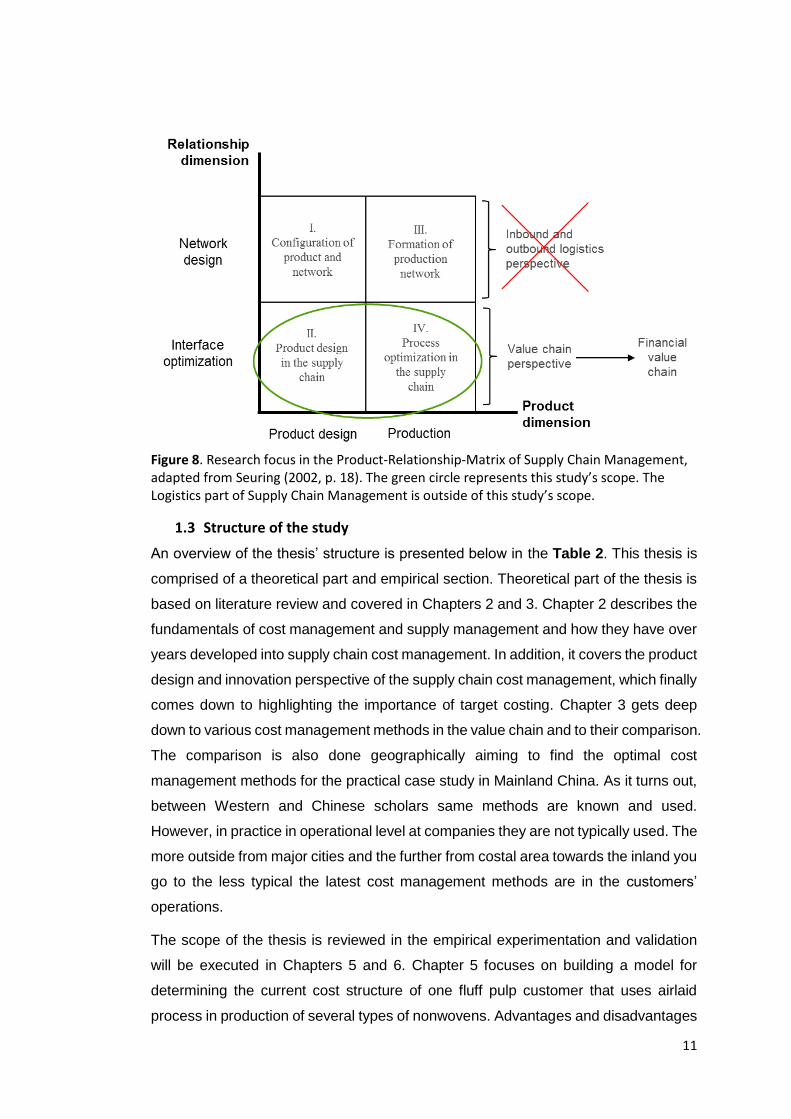
11
Figure 8. Research focus in the Product-Relationship-Matrix of Supply Chain Management, adapted from Seuring (2002, p. 18). The green circle represents this study’s scope. The Logistics part of Supply Chain Management is outside of this study’s scope.
1.3 Structure of the study
An overview of the thesis’ structure is presented below in the Table 2. This thesis is
comprised of a theoretical part and empirical section. Theoretical part of the thesis is
based on literature review and covered in Chapters 2 and 3. Chapter 2 describes the
fundamentals of cost management and supply management and how they have over
years developed into supply chain cost management. In addition, it covers the product
design and innovation perspective of the supply chain cost management, which finally
comes down to highlighting the importance of target costing. Chapter 3 gets deep
down to various cost management methods in the value chain and to their comparison.
The comparison is also done geographically aiming to find the optimal cost
management methods for the practical case study in Mainland China. As it turns out,
between Western and Chinese scholars same methods are known and used.
However, in practice in operational level at companies they are not typically used. The
more outside from major cities and the further from costal area towards the inland you
go to the less typical the latest cost management methods are in the customers’
operations.
The scope of the thesis is reviewed in the empirical experimentation and validation
will be executed in Chapters 5 and 6. Chapter 5 focuses on building a model for
determining the current cost structure of one fluff pulp customer that uses airlaid
process in production of several types of nonwovens. Advantages and disadvantages
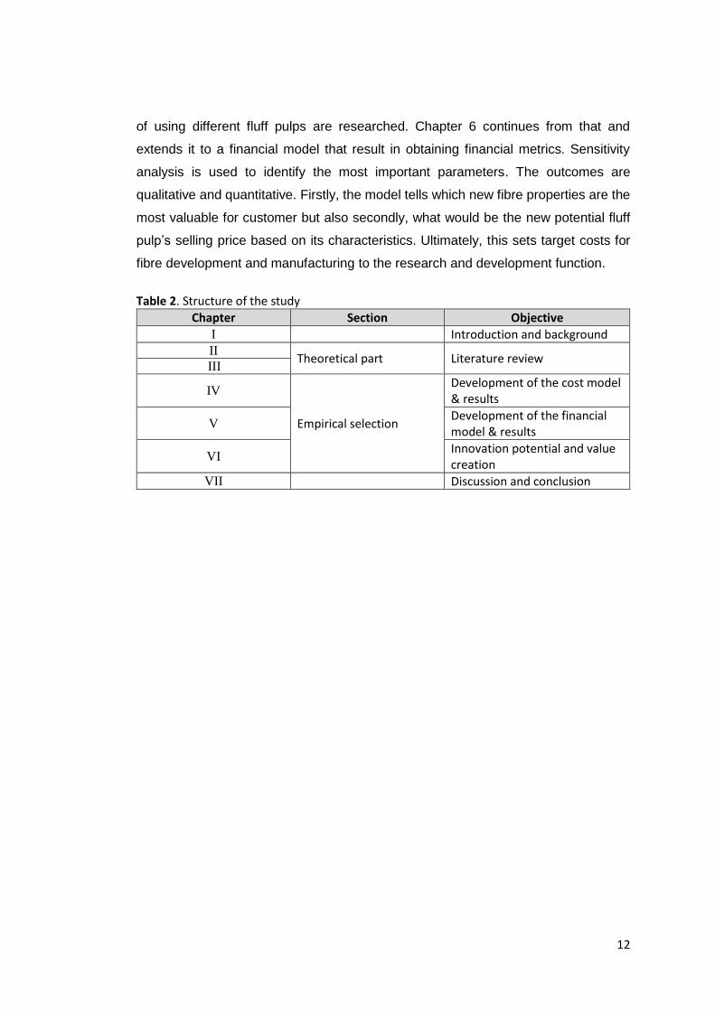
12
of using different fluff pulps are researched. Chapter 6 continues from that and
extends it to a financial model that result in obtaining financial metrics. Sensitivity
analysis is used to identify the most important parameters. The outcomes are
qualitative and quantitative. Firstly, the model tells which new fibre properties are the
most valuable for customer but also secondly, what would be the new potential fluff
pulp’s selling price based on its characteristics. Ultimately, this sets target costs for
fibre development and manufacturing to the research and development function.
Table 2. Structure of the study
Chapter Section Objective I Introduction and background II
Theoretical part Literature review III
IV
Empirical selection
Development of the cost model & results
V Development of the financial model & results
VI Innovation potential and value creation
VII Discussion and conclusion

13
2 Supply chain management
The scholars and practitioners have struggled with the definition for supply chain
management from the early stages of the field’s evolution. From logistics before
1950s it has also been variously referred as distribution, physical distribution, logistics,
business logistics, integrated logistics, materials management, value chains and
rhocrematics which is a Greek term referring to the management of material flows.
The logistics as a field has a strong military history when it had to do with procurement,
maintenance and transportation of different military facilities, material and personnel.
The firms back in then were interested in getting right goods to right place at the right
time and hardly no research was done on trading one cost for another. Other areas
were thought to be more important. Hence, there was not even opportunity to learn
broader concepts of logistics or beyond.
The concept of logistics and the field that eventually has shaped into supply chain
management developed from the marketing field. Lalonde and Dawson (1969) traced
the early history of logistics and note that Arch Shaw in 1912 saw the two sides of
marketing where one deals with demand creation (promotion) and the other with
physical supply. First the distribution seemed to be part of the marketing mix and was
defined more in terms of transaction channel activities than physical distribution ones.
Companies still in 1950s and early 1960s paid a great deal more attention to buying
and selling than to physical distribution.
The kick off for laying foundations for physical distribution was made by Lewis et al.
(1956) in a study for the airline industry. The airline industry was thinking how it could
better compete in hauling flight even when their costs were significantly higher than
other forms of transportation. The study found out that it is necessary to view shipping
from a total cost perspective and not from just a transportation cost one. Although
airfreight cost was typically higher, airfreight’s faster and more reliable service led to
lower inventory costs on both ends of the shipment. This lead to the total cost concept
in logistics, which began to take off in the 1960s. The focus was on firms’ outbound
logistics and little attention was given to inbound material movements.
In 1964, the scope of physical distribution was expanded (Heskett et al., 1964) to
include physical supply and was called business logistics. Using a descriptive name
of business logistics was not only an attempt to distinguish the name from military
logistics but to focus on logistics activities that took place within the business firm.

14
In the 1060s and 1970s the study and practice of physical distribution and logistics
emerged spurring by the recognition of high logistics costs and therefore got
managerial attention. It was estimated that on a national level logistics costs in the
USA accounted for 15 % of the gross national product (Heskett et al., 1973). Similarly,
in UK, they were 16 % of sales (Murphy, 1972), in Japan 26.5 % of sales (Kobayashi,
1973), in Australia 14.1 % of sales (Stephenson, 1975), and as of 1991 in China they
were 24 % of GDP. Physical distribution with its outbound orientation was first to be
laid focus on, since it represents about two thirds of logistics costs. Subsequently,
business logistics, including inbound movement followed soon after that.
Heskett et al. (1973, p. 25) recognized that logistics takes place throughout the supply
channel, from producer to end consumer. Heskett et al. (1973) also suggested that
there needs to be coordination of the product flows throughout the entire channel,
which is probably the first implication of what SCM is described now. The early
definitions already suggested a broad scope for the physical distribution and logistics
but still the focus was on coordinating among the activities within the logistics function
and giving little emphasis on coordinating among the other functions within the firm,
not to mention with the external channel member. The reason for this is most likely
technical limitations of information systems at the time. Coordination between
business functions was to become a major theme in later years starting from late
1970s and early 1980s. This can be seen from the interfunctional and
interorganizational coordinative functions in Figure 9: Strategic planning, information
services, marketing/sales and Finance.

15
Figure 9. Evolution of supply chain management from 1960 to 2000 and beyond (Ronald , 2007, p. 338)
The Council of Supply Chain Management Professionals (CSCMP), which is the
organisation of supply chain practitioners, researchers and academics, has defined
SCM as:
“Supply Chain Management encompasses the planning and management of all
activities involved in sourcing and procurement, conversion, and all Logistics
Management activities. Importantly, it also includes coordination and collaboration with
channel partners, which can be suppliers, intermediaries, third-party service providers,
and customers. In essence, Supply Chain Management integrates supply and demand
management within and across companies.”
Whereas, CSCMP defines logistics to be just one part of SCM:
“Logistics management is that part of SCM that plans, implements, and controls the
efficient forward and reverse flow and storage of goods, services, and related
information between the point of origin and point of consumption in order to meet
customer requirements.”
Therefore, nowadays SCM is viewed as managing product flows across multiple
companies and logistics is considered as managing the product flow activities just
inside one company. Seeing it in a big picture, a contemporary view of SCM is to think
of it as managing a set of processes, where a process is a group of activities in
16
functions throughout the entire supply channel relevant to achieving a defined
objective, which is typically a customer need, whole product or service to the end
customer. Saying that, the contemporary view is that SCM is a new frontier for
demand generation – an effective competition tool. Figure 10 presents how SCM can
be used as a tool for reaching business competitiveness. On the same time, it
illustrates the divergence of SCM and supply chain cost management (SCCM). SCCM
is a subcategory of SCM and serves as a tool to reach SCM objectives. Theory of
SCCM is covered in Chapter 3 but first it is described how to combine SCM and
SCCM.

17
Figure 10. The divergence and connection point of supply chain management and supply chain cost management (adapted from (Ansari, et al., 1997; Archie & Wilbur, 2000, p. 214)
When looking at a typical product life-cycle of a nonwoven or absorbent product over
the years it becomes clear that the trend is for reduced lifetime and increased
differentiation in the downstream. A product’s lifetime is an attribute of new product
introduction rates and intervals between new product generations. This has been
especially true in electronics but nowadays also in fast moving consumer goods
(FMCG), causing the product design and development phase to become more

18
pronounced when overall production costs are examined. For the pulp industry the
production development cost has been low in relation to many other industries where
product development itself can incur significant costs; from 3 % to even 25 % and
average being 9 % of total costs. However, its activities can significantly impact on
production costs of pulp and the whole end-product along the value chain. A big
portion of the costs can be influenced in the production development phase. By this,
the feasibility of a development action depends on gained benefits in the value chain.
This is where the whole supply chain perspective rises its importance affecting heavily
to operational and configurational efficiency. Not only the existing pulp value chains
are known to have price sensitive markets but also the potentially substitutable
synthetic raw materials are known to be price competitive.
The competitive landscape reflects to the whole product design process by the fact
that the whole chain needs to be optimized, when creating a new product. For
effective supply chain management to occur, firms must adopt a new managerial
approach (Balsmeier & Voisin, 1996) meaning that in contrast to anterior optimization
which happened on local objectives, companies should take a broader perspective in
supply chain management. New cost management systems need to be more focused
on maximizing customer satisfaction over minimizing local costs. In traditional
approach decisions are made without regard to their effect on other components of
the chain resulting in inability to fulfil company-wide objectives, conflicts between
functional areas and at the end of the day failure in meeting customer satisfaction.
For example, Ellram (1991) points out that the goal of supply chain management
should be to improve customer satisfaction at reduced overall costs not just local
costs.
The starting point for the supply chain management is presented in the Table 3, which
describes the typical cost structure of a 600 kt/a softwood chemical pulp mill cost
structure. For fluff pulp the chemical costs are a bit higher than for normal chemical
pulp because of the chemical debonders added during production to make it easier
(lower energy) to defiberize the fluff pulp in the hammermill prior to use. The total cost
is around 475-550 €/ton including delivery (Diesen, 2007).

19
Table 3. Typical cost structure of a 600 kt/a softwood chemical pulp mill at full production (Diesen, 2007) 1. Variable Costs %
Wood 31.0 Chemicals 7.9 Energy 0.7 Operating Material & Services 10.7
Total Variable Costs 50.3
2. Fixed Costs Maintenance Materials 5.2 Personnel & Administration 3.3 Others 5
Total Fixed Costs 13.5
3. Capital Costs 36.2
Total Costs 100
The next step for analysing the supply channel’s total costs would be to know the
buyer’s costs. By this performing a cost-benefit analysis in the value chain as
presented in the Figure 11 we would know in which research and development
actions to focus on if maximized benefits are sought. For example, if the research and
development function were able to modify the fluff pulp in a way that it would reduce
the latex binder consumption on fluff pulp buyer’s side, what would be the overall
monetary benefits in the value chain? Derivate of the value chain cost curve would
show the optimal situation.
Figure 11. Illustrative total cost in the supply channel
20
2.1 Supply chain management meets cost management
There are various ways companies and researchers have approached cost
management in supply chains. Researchers and practitioners started with traditional
cost management and moved into activity-based management (ABM), including
mostly activity-based costing but also in some cases time-driven activity-based
costing. Recently the focus has switched towards target costing (Smith & Lockamy,
2000) and its combinations with other methods, mostly with ABC. The main criticism
levelled against traditional cost management system is that it often solely focuses on
reducing costs in many different unconnected local levels. Some firms have attempted
to mitigate this problem by using activity-based management instead. However, it
does not remove the problem that it fails to address the issue of how the whole supply
channel could be utilized to reduce costs or increase customer satisfaction.
Companies utilize financial data from their cost management systems to plan and
control the operations of their supply chains. Over the time, they can deepen this
knowledge by establishing the costs of products and services and their alternatives
that are moving through the supply chains (Jonson, 1994, p. 18). Unlike in the optimal
supply chain (Figure 12) where the information flow of demands and design
information goes from the downstream to upstream, the information does not convey
to other participants of the supply channel in the traditional approaches. Due to these
facts, researchers and companies have slowly moved over to target costing, which is
considered as a better choice for supply chain (cost) management. In target costing,
costs are perceived as a result, whereas customer requirements are seen as binding
competitive constraints (Smith & Lockamy, 2000). The result is a method where
supply chain incurs costs that are necessary to satisfy customers’ expectations for
functionality and price, resulting in more competitive products as seen in Figure 10.
The Chapter 3 discusses all the cost management systems, their popularity in China
and the benefits and drawbacks of using them.

21
Figure 12. Supply chain material flow in an optimal case (Adapted from APIC/CPIM (1997) & (Wilbur & Lockamy, 2001)
2.2 Product design and innovation perspective in supply chain management
Supply chain management covers strategic, tactical and operational elements that
provide companies a wide span of different possibilities to maintain competitiveness.
Research and development is an important part of this. Recently supply chain
management development initiatives have been categorised mainly into two
categories: logistics innovation (LI) and supply chain innovation (SCI) (Munksgaard,
et al., 2014, p. 50). Putting the two into the product-relationship-matrix of supply chain
management (Figure 8) the logistic innovation’s research focus positions itself to the
upper left and right corner. This is where network design, distribution and logistics is
covered. As an example of logistics innovation development initiative could be for
example logistics technologies (e.g. digital solutions such as: EDI, ERP, RFID) and
logistics programs (single or multi-level vendor-managed inventory (VMI), scan-based
trading cross-docking, etc.), which focuses on the network and its material flow.
Meanwhile, the supply chain innovation is more to do with the supply channel its
offerings to customer, of which this study is focused on. Supply chain innovation is a
concept that has been increasingly invoked in academic circles well as in practice in
recent years.

22
Based on literature review on SCI Arlbjørn et al. (2011, p. 9) put a following definition
of SCI: “Supply chain innovation is a change (incremental or radical) within a supply
chain network, supply chain technology, or supply chain process (or a combination of
these) that can take place in a company function, within a company, in an industry or
in a supply chain in order to enhance new value creation for the stakeholder.” In
addition, Arlbjørn et al. (2011) introduces three elements of SCI, namely supply chain
business process, supply chain technology and supply chain network structure or
compositions of these. The development of SCM is achieved through supply chain
innovation and logistic innovation.
The emphasis in SCI has recently drawn into value, some researchers referring it as
value-based supply chain management making the supply chain cost management
more market oriented and value driven. Since the supply chain management is
achieved through supply chain cost management and supply chain innovation, value
creation and its measurement help to meet strategic objectives through research and
development department.
As addressed by Hofmann (2010), the key factors for successful differentiation and
competitiveness are proactive management within the supply chain, efforts strongly
related to supply chain innovation. Since the supply chain management is achieved
through supply chain cost management and supply chain innovation, value creation
and its measurement help to meet strategic objectives through research and
development department. According to Munksgaard et al. (2014, p. 51) value created
from supply chain innovation is primarily cost driven. Slater (1997) envisions value to
be the difference between benefits derived and sacrifices and/or costs incurred.
According to Porter (1985, p. 38), value is “the amount buyers are willing to pay for
what a firm provides them.” This claim is backed by various researchers and stated
that value is conceptualized and measured using monetary terms. However, some
researchers (Slater, 1997; Willson & Jantrania, 1998; Amit & Zott, 2001) have stated
that value could also include things like competence, effectiveness, differentiation and
social rewards, which are non-monetary aspects. Given this, value could be
envisioned more broadly as the difference between benefits derived and sacrifices
and/or costs incurred (Slater, 1997). These benefits (read: value addition) might
extent even to creation of new markets (Munksgaard, et al., 2014, p. 53). Therefore,
sources of value do not exist within a firm’s boundary alone, contrary, to create
superior value, organizations are strived to understand their entire value chain
extensively.

23
2.3 Target costing in supply chain management
Cost efficiency and partly success for firms depends on their ability to balance a
stream and process changes with meeting customer demands, improving cost,
delivery, service and product quality and delivery flexibility. In other words, the
success depends on how a firm performs Figure 10’s supply chain management
activities. This happens across different organisational functions, companies and
national borders. Managing these effectively requires. In order this to happen
effectively Balsmeier and Voisin (1996) started the swift from traditional operating
method to a new managerial approach. Increasing competition is forcing companies
to go away from managing each segment as an independent entity and concentrating
on achieving local objects. Today’s value chains are taking into account their effect
on the down or upstream value chain and looking the costs structure as a whole.
Therefore, the success of value chains depends on how by coordination the network
of firms are able to fulfil the end-customer needs better than other competitive value
chains. Not anymore just companies but also value chains are competing.
A primary reason for the failure of traditional approach was its dependence a cost
management system that is focused on minimizing local costs over maximizing
customer satisfaction (Archie & Wilbur, 2000, p. 210). This method works against of
SCM’s ultimate goal of increase customer satisfaction of which only one way is the
minimization of costs among several other ways. Saying this, solely using traditional
approach and ABM the SCM would fail to utilize other ways than cost minimization to
increase customer satisfaction. Target costing focuses less on costs than on
customer requirement. Customer requirements are seen as competitive constrains of
which have to be first met and subsequently met as cost effective as possible. Instead
of cost minimization, the cost rationalization as a function of customer satisfaction is
sought.
Cost estimation and reduction have always been a great concern in a product design
cycle (Romero Rojo et al. 2009). In recent years, research aim has been focused on
two aspects in product development improvement: how to shorten the product
development and how to reduce the product development cost. This is due to
contemporary global manufacturing environments that require agility, yet applying the
state-of-the-art technology to respond to various customer requirements, needs, and
wants. Typically, costs considered under product development costs are the sum of
the costs in product design, production and logistics. Overhead costs are usually
taken into account, in practice with an estimation by multiplying the product

24
development cost by a constant variable. The product design cost normally
determines the achieved market share, profitability and return on investment that is
why accurately estimated costs play vital part while influencing to the selection of a
mix of production development processes which can completely meet customer
requirements with a lowest sum of costs. Accurate estimation and optimal controlling
the cost of product design is crucial to shorten product development cycle and reduce
its cost.

25
3 Supply chain cost management methods
Supply chain cost management has divided to its own sub-research category from
supply chain management and gotten influence from cost management (also referred
as management or managerial accounting). In fact, cost reduction has been among
the most cited objectives in supply chain management research over the recent years.
Both supply chain management and cost management are platforms for a wide variety
of methods, concepts and instruments. Therefore, looking at the intersection of those
two, which is called supply chain cost management, does not lead to a single, clear
concept. Therefore, it is important to clarify what is supply chain cost management
and how it has evolved in the presence of cost management and its methods. It is
noteworthy that still many researchers categorise cost management activities in
supply chain straight under supply chain management, not under its specific field of
supply chain cost management. Some even put it under strategic management
accounting or cost/managerial accounting.
In the past, researcher used developed instruments that were evolved from
management accounting to treat intercompany historical data. However, this was
insufficient, and the focus has shifted on more real time evaluation methods. Instead
of only arranging past data, according to Dellmann & Franz (1993) “the present cost
data within the value chain must be assessed, planned, controlled and evaluated”.
The need for real time and future oriented decision-making lead to development of
concepts further than management accounting, for example concepts like generally
most recognised target costing, activity-based costing and life-cycle costing. On the
same time, the broadness of supply chain cost management has moved from
intercompany perspective towards more integrated supply chain operation where
development areas are looked from supply channel perspective. The force for this
change has been an increasingly intense competition of profits. For cost allocation,
this has meant that it has had to undergone changes to better meet managers’ needs
of aiming higher competitiveness. What this has mean in practice is for example more
value-based activities and decision-making. As Gupta & Gunasekran (2005) states
the role of managerial accounting in a new enterprise environment: “One of the critical
roles of managerial accounting is to identify and eliminate . . . non-value adding
activities throughout the value-chain.” Successful fusion and management of
26
accounting and decision-making is a major competitive edge in the 21st century
(Drucker, 1992) .
Currently, most of the cost systems are based on traditional operating principles and
concepts (Jonson and Kaplan, 1987, p. 12) and the transition out from these has been
rather slow. However, activity-based management has gained popularity and is
expected to do so even more. In Table 4 the evolution of cost measures is presented.
It should be noted that the scholars are always the first movers and for practitioners
it typically takes more time to implement a new way of operating. In addition, there is
variation geographically as well. The next sections of the research discuss some of
these systems more detailed, their popularity in China and the benefits and
drawbacks of using them.
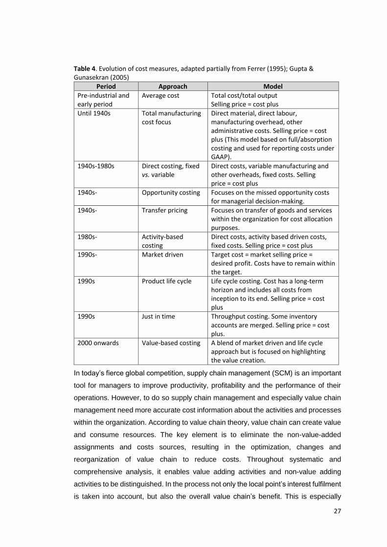
27
Table 4. Evolution of cost measures, adapted partially from Ferrer (1995); Gupta & Gunasekran (2005)
Period Approach Model
Pre-industrial and early period
Average cost Total cost/total output Selling price = cost plus
Until 1940s Total manufacturing cost focus
Direct material, direct labour, manufacturing overhead, other administrative costs. Selling price = cost plus (This model based on full/absorption costing and used for reporting costs under GAAP).
1940s-1980s Direct costing, fixed vs. variable
Direct costs, variable manufacturing and other overheads, fixed costs. Selling price = cost plus
1940s- Opportunity costing Focuses on the missed opportunity costs for managerial decision-making.
1940s- Transfer pricing Focuses on transfer of goods and services within the organization for cost allocation purposes.
1980s- Activity-based costing
Direct costs, activity based driven costs, fixed costs. Selling price = cost plus
1990s- Market driven Target cost = market selling price = desired profit. Costs have to remain within the target.
1990s Product life cycle Life cycle costing. Cost has a long-term horizon and includes all costs from inception to its end. Selling price = cost plus
1990s Just in time Throughput costing. Some inventory accounts are merged. Selling price = cost plus.
2000 onwards Value-based costing A blend of market driven and life cycle approach but is focused on highlighting the value creation.
In today’s fierce global competition, supply chain management (SCM) is an important
tool for managers to improve productivity, profitability and the performance of their
operations. However, to do so supply chain management and especially value chain
management need more accurate cost information about the activities and processes
within the organization. According to value chain theory, value chain can create value
and consume resources. The key element is to eliminate the non-value-added
assignments and costs sources, resulting in the optimization, changes and
reorganization of value chain to reduce costs. Throughout systematic and
comprehensive analysis, it enables value adding activities and non-value adding
activities to be distinguished. In the process not only the local point’s interest fulfilment
is taken into account, but also the overall value chain’s benefit. This is especially

28
important in design stage in the current markets but also in new market exploration
when analysing the potential new market and specifying the competitive advantage
possibilities over existing players. The idea behind this optimization is that we are able
to create a simulation model based on a determined cost method. The model could
easily determine profitability of the concept product of which properties are defined to
meet certain consumer segment needs and thus create winner value chains.
3.1 Traditional costing
Traditional costing method, which refers to total manufacturing cost and direct cost
(used from the early industrial period to 1980s), evolved from the average cost
method. Whereas in the average cost method, total cost is divided by the total output,
in total manufacturing cost the total cost is broken down into direct (material and
labour) costs and indirect (manufacturing and overhead) costs. The indirect costs are
estimated by averaged over single or multiple cost pools. Based on a cost driver,
which can be for example, direct labour, material, or labour or machine hours, are
used to determine individual product cost. The traditional costing and accounting
system was designed to capture the operational costs by using the Generally
Accepted Accounting Principles (GAAP). These calculations were used in the basis
for financial statements referred as financial accounting. The traditional costing
method suited well for the needs of the times as early as 1850s. These management
control systems provided much needed coordination, control and discipline for large
enterprises that time. However, in the new enterprise environment in 21st century
these measures are lagging behind on decision-making and lack predictive value.
Moreover, they lack of strategic and operative measures. These measurements
should be able to influence the business processes and add value, which are in line
with the strategic goals of the enterprise.
It is concerned that traditional costing has several drawbacks: (1) traditional costing
does not provide adequate relevant non-financial information, (2) traditional
accounting results in inaccurate product costs, (3) traditional accounting does not
encourage improvement and (4) traditional costing fails to allocate overhead costs
(Gupta & Gunasekran, 2005). One of the critical roles of cost management is to
identify and eliminate non-value adding activities, which the traditional cost fails to
address. The importance of this increases when going from inner-company to an
inter-company perspective, where the costs effect amplifies throughout the supply
channel.

29
3.2 Activity-based costing
There are two ways of proceeding activity-based costing, first called the traditional
way which was introduced in 1987 and the second a simplified version of this called
time-driven activity-based costing. Initially the activity-based costing (ABC) was a
reply to inaccurate American accounting standards (Kuchta & Troska, 2007). This
new method was concerned with what was done in terms of activities instead of
traditional thinking of what was spent. This new method can support management,
planning and decision making, which is critical in ever changing market and
competitive markets that companies face when doing international business. Activity-
based costing introduced by Johnson & Kaplan (1987) has gathered many supporters
along the years. The main difference to traditional costing is the number of cost pools
and the variety of cost drivers (Shannon & Don, 2008), illustrated in Figure 13.
Kennedy (1996) explains this simply in his article that ”the activity cost pool is the
overall cost associated with an activity” and continues “a cost driver is a feature that
allocates the cost and performance to a certain activity. By applying activity-based
costing, implementing cost tracing throughout the whole value chain is possible: from
sourcing and manufacturing (Korpunen, 2015) towards supply chain (Koivula, 2015)
to all the way to a retailer and end consumer profitability analysis (CPA) (Wei, 2011).
Therefore, a well-designed ABC system is a powerful aid to management evaluation
and decision-making, thereby in long term, it is an invaluable tool for improving
organizational performance. In fact, Cagwin & Bouwam’s (2002) results showed that
there is a positive association between ABC and improvement in ROI and overall
improvement in financial performance.
The most likely reason for improved financial performance is that the features gained
from applying ABC can be used beyond status quo manufacturing and supply chain
activities. At the turn of the millennium, researchers began to examine its usability to
estimate the manufacturing costs modelling of a product that is in a conceptual design
and development stage. There are already several doctoral theses made on this
subject; Tornberg et al. (2002) made an Activity-based costing model specially for
cost-conscious product design “for the evaluation of different product design options”
and concluded that “activity-based costing and process modelling provide a good
starting point” when product design team aspire to more cost-conscious product
outline. This is due to the fact that designers become aware of relationships between
the activities performed during the manufacturing and their associated costs in more

30
detailed. Identifying non-value adding activities or product features pose a major cost
reduction potential.
There is a major weakness of activity-based costing when designers want to specially
track certain product feature costs. Tornberg et al. (2002) mention that there is “a risk
for calculations to include too many activities. This makes the calculations too
complicated and too slow to use. This might be major problem, because product
designers might demand for detailed information. Solution for this Tornberg et al.
suggest a model should have different levels of information, which gives possibility to
get more detailed information, while still allowing quick overall picture of the overall
situation. This could be done by categorizing activities into larger groups and
aggregate them by certain cost nature, for example to life-cycle activities that could
include activities such as life-cycle maintenance costs, life-cycle manufacturing costs
and so forth.
There are several problems associated with the data gathering. Firstly, survey
approach is recommended, however the data gathered by this way is always
subjective and difficult to validate. Importing the data from management information
system’s data is not very often readily usable, accurate or even existing as the amount
of data required is huge, which is expensive to store, process and report (Namazi
2016). Rolling this method on an frequent basis in a large scale requires rather lot of
work. In some companies this has led to a situation where cost modelling systems
are updated infrequently due to costs of reinterviewing and resurveying. This had led
to outdated and inaccurate cost information leading the process, product, and
customer costs become inaccurate. In addition, the model is theoretically incorrect
while it ignores the potential of unused capacity (Namazi 2016).
In many real-life cases there are many ways of performing an activity, for example
various ways to ship an order to customer. Traditional ABC models often fail to
capture this complexity of actual operation while not allowing significant variation in
resources required, incurring new activities to be added into the model. This increases
its complexity meaning that in many cases such expansion of ABC systems has
exceed the capacity of typical generic spreadsheet tools, such as Microsoft Excel, but
also even many ABC software packages. However, these runnability problems arise
only when months’ worth of data is processed. For product development purposes
this approach might prove to be too laborious.

31
The following stages can be concluded for Activity Based Costing (Cooper and Kaplan
1998; Bruggeman and Everaert 2007; Krumweide 1998):
1) Collecting data on resources 2) Identifying activities 3) Defining the cost of the activities 4) Defining the cost drivers of activities 5) Defining the volume of cost drivers 6) Defining unit cost per cost driver for each activity and 7) Calculating the unit cost per product or service
Creating a new ABC system begins with collecting data on resources in which the
focus should be on expensive resources, mostly the direct labour and materials cost.
It is important to pay attention to resources that varies significantly on consumption
by product. In addition, the focus should be on resources whose demand patterns are
different compared to traditional allocation measures. These are typically direct labour,
processing time and materials used. After that activities are identified and categorised
as value adding and non-value adding activities. Subsequently the costs and cost
drivers of activities are defined. Cost drivers are based on determined cost driver
activity units. After this the volumes i.e. consumption of each cost drivers are
determined. Second to last, the unit cost per cost driver can be calculated by dividing
the activity’s total cost by the cost driver volume. Finally, the unit cost is calculated by
multiplying the cost per cost drivers by their corresponding activity consumptions. The
whole process can be also seen from Figure 13.
Table 5. Advantages and disadvantages of activity-based costing
Advantages Disadvantages
More accurate cost per unit improved sales strategy, performance management and decision making.
Examines the actual overhead cost drivers instead of the assumption of production volume relation.
Can be applied to all overhead costs, not just production overheads.
Enables costing model’s complexity bringing higher cost estimation accuracy.
Ability to implement into supply chain environment.
Enables costing from a product design and innovation perspective.
Limited benefit if the overhead costs are primarily volume related or if the overhead is a small proportion of the overall cost.
Requirement of allocating all the overhead cost to specific activities.
Might be more complex to explain to stakeholders.
Time consuming when building a model and maintaining it.
Requires sophisticated information technology, highly competitive environment, relatively high importance of costs, relatively low unused capacity and little intra-company transactions.

32
Advantages Disadvantages
Activities can be categorized into value creating and non-value creating segments.
Decision making level can take place even by product level
Relies on managerial estimations of cost driver consumptions (data reliability).
Ignores unused capacity and variations in activities.
Activity based costing is very good in addressing the deficiencies the model reveals
including inefficient processes, unprofitable products and customers but also excess
capacity.
Figure 13. Illustration of three costing methods: traditional costing, activity-based costing and time-driven activity-based costing
3.3 Activity-based costing from a product design perspective
In their doctoral thesis, Tornberg et al. (2002) focused their attention specially on two
of eleven main problems Uusi-Rauva and Paranko (1998) identified when interviewing
accounting professionals (information producers) and product design managers
(information users). These two were both around the same topic about how product
designers would get more information about indirect costs but also better
understanding of the direct cost dynamics. First, information from product structure
and business process activities should be better combined. Second, product
designers need more accurate and reliable cost information on product’s total costs.
3.4 Time-driven activity-based costing
A problem for many companies that have tried to implement Activity based costing in
their organization on any significant scale is that they have faced rising costs and
employee irritation and therefore had abandoned their attempt. The time-driven

33
activity-based costing were developed to give a solution for this. The method relies
managerial estimates rather than on employee surveys, which might get too laborious.
To build a traditional ABC model for a department, one would need to survey
employees to estimate the percentage of time they spend on all the activities and then
assign the department’s resource expenses according to the average percentages
gotten from the survey (Kaplan & Anderson, 2004). The TDABC makes allocation
easier allowing even cost simulation model building in the product development phase.
In addition, the decision-making process in ABC becomes to take place more at the
product level, meaning that it is based on actual utilization and does not identify the
vacant capacity, whereas in time driven activity-based costing decisions are taken
place on both production and process level. Kaplan and Anderson’s (2004) article
claims that even if in Time Driven Activity Based Costing activities are not taken into
account, it still provides more accurate cost-driver rates, because unit times can be
estimated even for complex and specialized transactions.
Namazi (2016) composes in his doctoral thesis different perspectives on time-driven
activity-based costing. The study reports time driven activity based costing’s
applications in several strategic areas such as production cost, unutilized capacity,
price setting, analysing customer profitability, and modelling complex decisions in
various SMEs and large private companies, governmental companies, nonprofits and
heavy manufacturing organizations.
3.5 Lean Accounting
The lean concept is a philosophy in which non-value-adding activities are recognized
and eliminated in lean manufacturing systems. Lean accounting as a term refers to
systematic methods that were developed for financial management based on lean
principles. These methods have been standardised and in 2005 leaders in Lean
Accounting reached to an agreement on a document named “The Principles,
Practices and Tools for Lean Accounting. The quintessential idea of this is to aim at
reduced cost over removal of waste, this is done with simplifying manufacturing
processes (Blackstone et al. 2005). This leads to non-value-adding activities to be
removed. Interestingly Time Driven Activity Based Costing were introduced just a
year before in 2004, one might claim that the publication of standardised method for
Lean Accounting document was a counter answer to the improved version of Activity
Based Costing. According to Kennedy and Maskell (2007) Lean Accounting methods
and tools support three key aspects of a lean organization: visual management, value

34
stream management and continuous improvement. Value stream costing tools and
target costing has been widely implemented in Lean Accounting and according to
several papers it is a good tool for guaranteeing customer satisfaction.
Table 6. Different approaches summary for information generated from each accounting system (Adapted from Monroy et al. (2012))
Activity Based Costing
Time-driven activity-based costing
Lean accounting
Financial reporting Not accepted by GAAP
Not accepted by GAAP
Accepted by GAAP
Decision making Takes place by product level
Takes place at product and process level
Takes place at value stream level
Operational control and improvement
Emphasis on financial measures
Emphasis on nonfinancial measures
Emphasis on nonfinancial measures
New product development
Suitable Most suitable Suitable for value chain cost perspective
Activity-based costing and time-driven activity-based costing are not accepted by
GAAP, however, ABC by itself usually has little or no impact on the structure of the
firm's financial accounting reports. This is because all the accounting methods no
matter if it ABC, TDABC or traditional costing ultimately assign costs to the same
existing accounts.
As a conclusion, one cannot obtain a perfect model just by applying one cost model.
However, after being aware of the benefits and restrictions these can be taken into
account and choose the most suitable model for each situation.
3.6 Life-cycle costing
The life cycle costing (LCC) analysis is an engineering and economic optimization
technique, in which the main target is to identify and choose the option which
maximises the generated revenue over the product’s lifetime. On a parallel, this
means also lowest lifecycle cost generation (Fabrycky & Blanchard, 1991).
3.7 Target costing
Target costing is a market-driven system for cost reduction, focused on managing
costs at the development and design stages of a product. It was developed in Japan
in 1970s by Toyota and has been successfully used there since. However, the
principles were well-known already before that, for example, back in the 1930s

35
Volkswagen set the sales price fixed from the start and implemented customer-
orientated approach. It still took almost half a century to use target costing in
innovation process, but yet again inception took place in automobile industry by Audi
in the 1980s. From the very start it was a response to the intensification in competition
and thus the requisite of shortening the length and cost of new product’s development
process (Hessen and Wesseler 1994, p. 150). The first stage of target costing is
called market-driven costing. The basic principle of market-driven costing and its
relation the upcoming cost model is presented in Figure 14. Alongside with profit
margin there is one input parameter, target price, that needs to be known. The target
price is determined based on market analysis and given the company’s target profit
margin, the target costing model gives target cost for the product.
Figure 14. The basic principle of target cost determination (Horvath et al. 1993)
After obtaining the target cost from market-driven costing, the process continues by
product-level target costing and component-level target costing (Figure 15). In these
steps, financial, manufacturing and customer aspects of the process are taken into
account.
The following process steps are subject to product-level and component-level target costing:
1. Determination of the overall costs 2. Breaking down the overall target costs into product individual components and
items (target cost breakdown) 3. Target cost implementation
When implementing the target cost, the object is to reduce cost by influencing to the
so called drifting costs. These are the cost that can be reduced. This stage will be
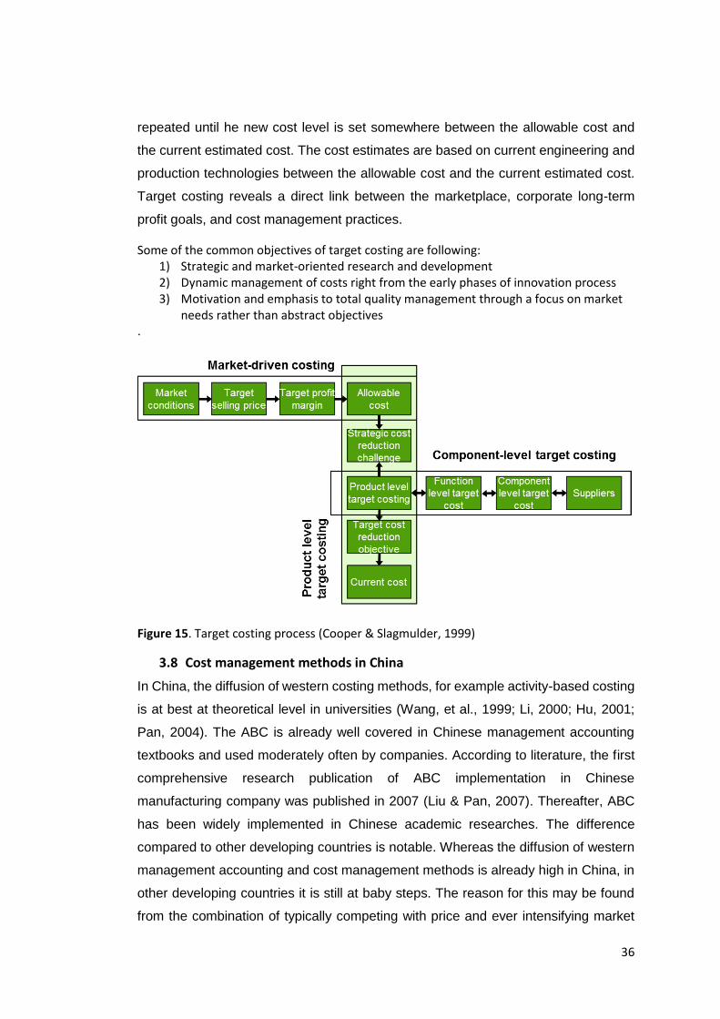
36
repeated until he new cost level is set somewhere between the allowable cost and
the current estimated cost. The cost estimates are based on current engineering and
production technologies between the allowable cost and the current estimated cost.
Target costing reveals a direct link between the marketplace, corporate long-term
profit goals, and cost management practices.
Some of the common objectives of target costing are following: 1) Strategic and market-oriented research and development 2) Dynamic management of costs right from the early phases of innovation process 3) Motivation and emphasis to total quality management through a focus on market
needs rather than abstract objectives .
Figure 15. Target costing process (Cooper & Slagmulder, 1999)
3.8 Cost management methods in China
In China, the diffusion of western costing methods, for example activity-based costing
is at best at theoretical level in universities (Wang, et al., 1999; Li, 2000; Hu, 2001;
Pan, 2004). The ABC is already well covered in Chinese management accounting
textbooks and used moderately often by companies. According to literature, the first
comprehensive research publication of ABC implementation in Chinese
manufacturing company was published in 2007 (Liu & Pan, 2007). Thereafter, ABC
has been widely implemented in Chinese academic researches. The difference
compared to other developing countries is notable. Whereas the diffusion of western
management accounting and cost management methods is already high in China, in
other developing countries it is still at baby steps. The reason for this may be found
from the combination of typically competing with price and ever intensifying market
37
competition. When competing with market shares and price, picking the right costing
method is an essential success factor. Taking these factors into account, the
traditional costing is inadequate and untrustworthy method to providing cost
information for managers. Thus, it is well justified to use Activity-Based Costing in
analysing and optimizing the cost structure. Providing accurate cost information on
how the sold product affects customer’s operations is highly appreciated in China.
In addition, Chinese management accounting, both academics and practitioners have
keenly implemented other innovative management ideas, particularly those that are
successfully adopted in the West (The implementation of Activity-Based Costing in
China). For example, Economic Value Added (EVA) and Key Performance Indicators
(KPIs) are well diffused and implemented (The implementation of Activity-Based
Costing in China).
In the last decade supply chain management has attracted much attention in many
Chinese industry sectors (Xu, et al., 2015). The focus has strongly been in
manufacturing and food industries, e.g. agriculture industry
3.9 Financial profitability evaluation methods
The simulation results of different pulp varieties are analysed by profitability
evaluation methods. Combination of various meters gives comprehensive picture
about the overall profitability. Net present value (NPV) is the difference between the
present value of cash inflows and the present value of cash outflows (Equation 1). A
positive NPV indicates that the projected earnings generated by a project or
investment exceeds the anticipated costs. In these cases, the time value of money is
taken into account. In other words, a sum of money earned in the future won’t be
worth as much as one earned in the present. There are several disadvantages in
using NPV while the result is highly dependable on the discount rate used. Companies
have different ways of identifying the discount rate. Common methods for determining
include using the expected return of other investment choices with similar level of risk
or the costs associated with borrowing money that is needed to finance the project
(Equation 6).

38
𝑁𝑃𝑉 = ∑
𝐶𝑡
(1 + 𝑟)𝑡
𝑇
𝑡=1
− 𝐶0 (1)
where:
Ct = net cash inflow during the time period
Co= total initial investment costs
r = discount rate, and
t = number of time periods
Payback period is an popular metric that is often implemented as an alternative to net
present value due to its simplicity. Unlike NPV, the payback method does not manage
to account money’s time value. Due to this, payback periods calculated for longer
investment periods have a greater tendency for inaccuracy. In addition, the payback
period fails to tell anything about the profitability of an investment after the investment
has reached the end of its payback period.
Modified Internal Rate of Return (MIRR)
𝑀𝐼𝑅𝑅 = √
FVCF(c)
PVCF(fc)
𝑛
− 1 (2)
Where: FVCF(c) = the future value of positive cash flows at the cost of capital for the company PVCF(fc) = the present value of negative cash flows at the financing cost of the company n = number of periods Economic value added (EVA) is an estimate of the value created (i.e. economic profit)
in excess of the required return of the company’s shareholders. As can be seen in
Equation 4, EVA is the net profit less the equity cost of the firm’s capital. EVA is able
to tell how much more, for example a process improvement, can improve the value a
company generates from the funds invested in it. Through this, it is possible to assess
whether the process improvement or investment is generating enough cash to be
considered a good investment. The greatest advantage of EVA is that it determines
whether the simulation creates wealth and returns for shareholders compared to the
cost of capital or not.

39
𝐸𝑉𝐴 = 𝑁𝑂𝑃𝐴𝑇 − 𝑊𝐴𝐶𝐶 ∗ (𝑡𝑜𝑡𝑎𝑙 𝑎𝑠𝑠𝑒𝑡𝑠 − 𝑐𝑢𝑟𝑟𝑒𝑛𝑡 𝑙𝑖𝑎𝑏𝑖𝑙𝑖𝑡𝑦) (3)
𝐸𝑉𝐴 = 𝑁𝑂𝑃𝐴𝑇 − 𝐼𝑛𝑣𝑒𝑠𝑡𝑒𝑑 𝑐𝑎𝑝𝑖𝑡𝑎𝑙 ∗ 𝑊𝐴𝐶𝐶 (4)
Where,
NOPAT = Net operating profit after taxes
WACC = Weighted average cost of capital
Return on capital employed (ROCE) is a financial ration that measures company’s
profitability and its capital employment efficiency. ROCE differs from EVA in
calculation as it uses earnings before interest and taxes (EBIT) instead of net
operating profit after taxes. EBIT tells more about company’s earnings without taking
into account interest or taxes. EBIT is calculated by subtracting cost of goods sold
and operating expenses from revenues. A higher ROCE indicates higher level of
capital usage efficiency. Both EVA and ROCE are especially useful when comparing
the performance of companies in various scenarios.
𝑅𝑂𝐶𝐸 =
𝐸𝐵𝐼𝑇
𝐶𝑎𝑝𝑖𝑡𝑎𝑙 𝑒𝑚𝑝𝑙𝑜𝑦𝑒𝑑 (5)
Where,
EBIT = Earnings before interest and tax
Weighted average cost of capital (WACC) is a calculation of a firm’s cost of capital in
which each category of capital is proportionally weighted. By calculating WACC and
comparing it to ROCE, we can understand how big of an benefit the customer got
from process improvement, related to cost of capital. In addition, WACC gives the
discount rate that should be used for cash flows that have similar risk inside the firm’s
other same type of projects. If the risk is estimated to be higher, also the discount rate
should be adjusted higher.
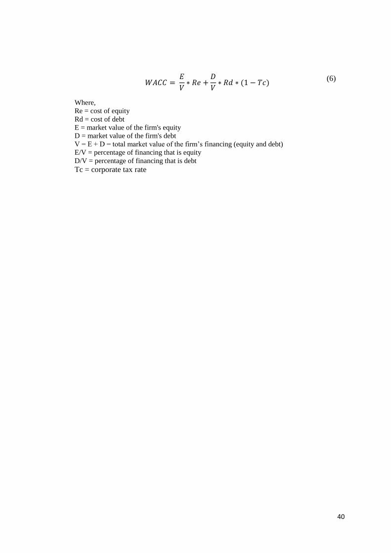
40
𝑊𝐴𝐶𝐶 =
𝐸
𝑉∗ 𝑅𝑒 +
𝐷
𝑉∗ 𝑅𝑑 ∗ (1 − 𝑇𝑐)
(6)
Where,
Re = cost of equity
Rd = cost of debt
E = market value of the firm's equity
D = market value of the firm's debt
V = E + D = total market value of the firm’s financing (equity and debt)
E/V = percentage of financing that is equity
D/V = percentage of financing that is debt
Tc = corporate tax rate

41
4 Development of the cost model
The critical role of product design in cost management is universally being recognized.
Cost modelling content and form should vary depending who is its “client”, in this study
the client is product design team whose decisions, according to various writers is
among the most aspects most important for company competitiveness on the markets
(Tornberg, et al., 2002). Specially for product designers the cost model should be built
in a way that allows accurate and fast cost estimation (Mengoni, et al., 2017) in an
early stage of product design keeping in mind the need for comparing different product
options between each other. Costs may be measured on a functional level, such as
total transportation or inventory holding costs, but this cost information remains too
aggregated. In some applications this might be enough but, in many cases,
substantially detailed reckoning is needed. Therefore, the objective is that broadly
defined costs could be further evaluated among the suppliers.
On the same time the model is intended to give certain scope for the product
designers about markets (cost structure, potential innovation impacts and the impact
throughout the value chain. One fictitious but figurative example of the model usage
could be following: preliminary research has pointed out several interesting products
that fulfils determined qualification criterion (sales volume, novelty, future’s growth
potential etc.) for moving the market research to further examination. The model is
used to gain understanding of the cost structure in the whole value chain and what it
takes to meet the already determined target cost obtained from the preliminary market
research. The next step is to understand product design team and innovation
department’s areas for potential cost reductions and what this would mean monetary
terms and key performance indicator wise for the whole value chain. If the target cost
is met the process should be moved to further
4.1 Requirements for the model
Considering the widespread of increasing cost pressure, the product development
process should be cost efficient. Therefore, the product development time and costs
must be reduced which is possible through dynamic cost feedback model. Second
important reason to shorten the development time is ability to rapidly respond to
changing markets and pose the ability for combing the most profitable new market
frontier(s) from wide arrange of different options. In practice, the success of a product
development process depends on three factors, namely: function fulfilment, keeping
the costs structure in leash and finally sticking with the schedule. Model should
42
specially be designed for giving a good idea of value chain partner’s cost structure
and profitability, and what factors affect it the most. After analysing these, the next
step is to determine how much value addition different kind of pulp provide to the
customer and finally what would be the value addition of totally new kind of pulp to
the customer in terms of cost savings, increased selling price or increased sells.
When applying target cost management in product innovation, the target cost needs
to be transferred to upper stream meaning that the target price should be determined
effectively after every participant in the value chain, not only in one stage of the value
chain. This procedure has a reverse action too. If the product concept cannot meet
the target cost under the set functions and product characters, the whole proses
needs to be revised. Getting to this step might require several iterations which
highlights the importance of rapid but accurate modelling. By implementing target
costing throughout the value chain, the market pressure is allocated to downstream
and upstream firms. Furthermore, it is important to analyse the overall efficiency and
profitability in order to understand the feasibility. This is done by several financial
metrics. These key performance indicators are reviewed in the end of Section 3 and
NPV, MIRR, EVA and ROCE were selected.
In addition, sensitivity for variations in parameters needs to be assessed to get better
picture on how set values of an independent variable impact on a chosen dependent
variables under a determined set of assumptions. This is done by screening which is
a particular instance of a sampling-based method. The objective is to identify input
variables that contribute significantly to the model’s output uncertainty, rather than
precisely quantifying values for sensitivity (for example by using variance). This gives
precise enough information for preliminary analysis about the risk factors but on the
same time has short duration and low computational cost compared with other
approaches.
4.2 Building the model
The very first step in building the model is a visit in the customer’s site and
understanding how they operate and what are their needs for the model. After several
meetings with the management team and production workers, it became clear that
they were most interested in researching possibilities of lowering their operational
costs with a new type of fluff pulp. For this reason, OPEX is where the modelling was
set to focus on more detailed. After visiting the mill site, the building of the Cost model
started.

43
Figure 16. Value chain partner’s main operations in end-product manufacturing
4.3 Modelling variable costs
The variable costs at the customer’s site were identified to mainly consist of
production cost related items. Figure 16 present the main operations in our value
chain partner’s manufacturing of airlaid nonwoven. In the first process step, fluff pulp
is infeed and defiberized with hammermill prior to forming. The fluff pulp used is fed
into hammermill in rolls unlike in many other pulp end use applications which are
delivered in bales. The customer had three individual hammermills where different
kind of fluff pulps can be used simultaneously. The hammermill tears up the fluff pulp
sheet and breaks fluff pulp into loose agglomerates of individual fibres. During this
process, so called loose fibres are generated, which further on in the process cause
waste, and impacts customer’s product quality and is extra cost. The model takes
waste cost into account as raw material consumption but also as a loss of production
and monetizes it by calculating the loss of profit. This is because in the ideal situation
the whole production capacity could be sold with a margin that is now lost due to the
waste. In addition, waste has a fixed waste management cost as currently the fine
particles have no feasible end use application.
After hammer milling the individual fibers are deposited on a moving belt, or “forming
wire” into a preliminary nonwoven web which thickness (mm) and basis weight (g/m2)
depends on the forming wire speed (m/s) also known as machine speed. The web
width (m) is kept constant.
Hammermillx3
Formerx3 Calendee-ring
Latex-binderaddition
Possiblecutting
Reeling Drying Drying
Fluff-pulpLatex-binder
EnergyEnergy
Endproduct

44
The hammermill and former combination functions as the first part of the cost
simulation model. The models work with the parameters described in the process
description. A screenshot of the model at this stage is presented in Figure 17.
Hammermill and former. Screenshot of the model’s hammermill and former input
variables in which a module for Product 1 can be seen. Due to customer’s wish the
actual fluff pulp brand and parameters used are undisclosed, i.e. the input variables
shown are for illustration purposes.
Figure 17. Hammermill and former. Screenshot of the model’s hammermill and former input variables
Identical modules are made for all the products (totally 5) the customer produces. In
addition, new kind of products can be added for example in a case where the
customer would start producing new kind of nonwoven from our fluff pulp and on the
same time keeping the old products. The data used is retrieved from “LookUp-Data
sheet” where the input variables are centralized and modifiable. The model’s variables
in hammermill and former are presented in Table 7.
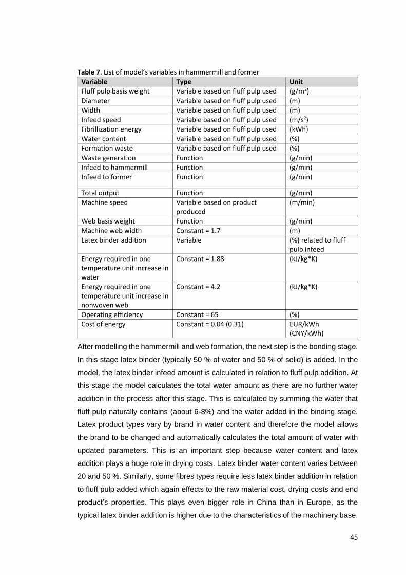
45
Table 7. List of model’s variables in hammermill and former
Variable Type Unit
Fluff pulp basis weight Variable based on fluff pulp used (g/m2)
Diameter Variable based on fluff pulp used (m)
Width Variable based on fluff pulp used (m)
Infeed speed Variable based on fluff pulp used (m/s2)
Fibrillization energy Variable based on fluff pulp used (kWh)
Water content Variable based on fluff pulp used (%)
Formation waste Variable based on fluff pulp used (%)
Waste generation Function (g/min)
Infeed to hammermill Function (g/min)
Infeed to former Function (g/min)
Total output Function (g/min)
Machine speed Variable based on product produced
(m/min)
Web basis weight Function (g/min)
Machine web width Constant = 1.7 (m)
Latex binder addition Variable (%) related to fluff pulp infeed
Energy required in one temperature unit increase in water
Constant = 1.88 (kJ/kg*K)
Energy required in one temperature unit increase in nonwoven web
Constant = 4.2 (kJ/kg*K)
Operating efficiency Constant = 65 (%)
Cost of energy Constant = 0.04 (0.31) EUR/kWh (CNY/kWh)
After modelling the hammermill and web formation, the next step is the bonding stage.
In this stage latex binder (typically 50 % of water and 50 % of solid) is added. In the
model, the latex binder infeed amount is calculated in relation to fluff pulp addition. At
this stage the model calculates the total water amount as there are no further water
addition in the process after this stage. This is calculated by summing the water that
fluff pulp naturally contains (about 6-8%) and the water added in the binding stage.
Latex product types vary by brand in water content and therefore the model allows
the brand to be changed and automatically calculates the total amount of water with
updated parameters. This is an important step because water content and latex
addition plays a huge role in drying costs. Latex binder water content varies between
20 and 50 %. Similarly, some fibres types require less latex binder addition in relation
to fluff pulp added which again effects to the raw material cost, drying costs and end
product’s properties. This plays even bigger role in China than in Europe, as the
typical latex binder addition is higher due to the characteristics of the machinery base.

46
Latex brand/product specific data is retrieved from the “LookUp”-data sheet. After
binding the excess water needs to be evaporated in order to get final product’s
targeted water content.
So finally, the drying/curing is carried out by using natural gas fired through air dryers
inside the drying unit. The typical end product’s targeted water content is 3 %. The
energy required can be calculated by estimating that the typical operating efficiency
of these type of drying units are 65 %. As a result, the model provides the user the
total amount of energy used in the production (except other energy costs that are
allocated as fixed cost) in energy units, euros per ton and per one minute of machine
run. The drying part of the model is introduced in Figure 18. Again, due to customer’s
wish, the numbers in the figure do not represent the real situation. Instead the
screenshot presented is captured from a simulated situation using figurative fluff pulp
properties and latex binder specifications and should be referred only to get better
understanding how the model works.

47
Figure 18. Latex binder addition and drying section
After modelling the production, starting from fluff pulp addition and hammer milling
costing and ending up to drying, the variable cost model lastly gathers all the cost
information and annual production levels of products into the same place. The cost
results are presented in Euros per tons and as a total figure, but the model also
calculates gross and net margin (€/ton & %) for all the products (Figure 19) after
retrieving the selling price from the “Vlookup” datasheet.

48
Figure 19. Total production, and summary of raw material usages and costs
At the end of the production line there would be still edge cutters and reeling but these
are taken into account in fixed cost costing while their cost character is closer to fixed
cost than variable cost.
4.4 Allocating and modelling fixed costs
Until this stage the costs determined and allocated to different products have
produced accurate cost information about the real situation, as the variable costs are
easier to identify, and problems do not really spring up in their allocation either.
However, a problem occurs when allocating these fixed costs. The fixed costs play
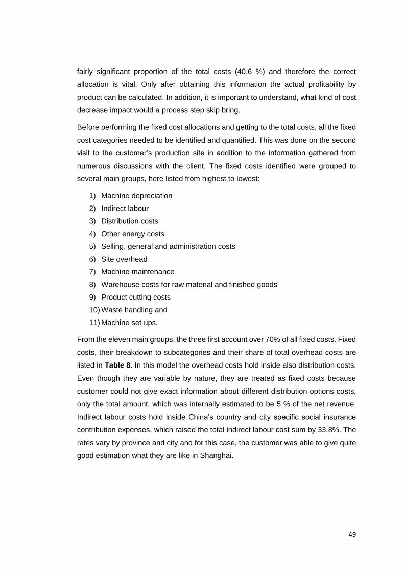
49
fairly significant proportion of the total costs (40.6 %) and therefore the correct
allocation is vital. Only after obtaining this information the actual profitability by
product can be calculated. In addition, it is important to understand, what kind of cost
decrease impact would a process step skip bring.
Before performing the fixed cost allocations and getting to the total costs, all the fixed
cost categories needed to be identified and quantified. This was done on the second
visit to the customer’s production site in addition to the information gathered from
numerous discussions with the client. The fixed costs identified were grouped to
several main groups, here listed from highest to lowest:
1) Machine depreciation
2) Indirect labour
3) Distribution costs
4) Other energy costs
5) Selling, general and administration costs
6) Site overhead
7) Machine maintenance
8) Warehouse costs for raw material and finished goods
9) Product cutting costs
10) Waste handling and
11) Machine set ups.
From the eleven main groups, the three first account over 70% of all fixed costs. Fixed
costs, their breakdown to subcategories and their share of total overhead costs are
listed in Table 8. In this model the overhead costs hold inside also distribution costs.
Even though they are variable by nature, they are treated as fixed costs because
customer could not give exact information about different distribution options costs,
only the total amount, which was internally estimated to be 5 % of the net revenue.
Indirect labour costs hold inside China’s country and city specific social insurance
contribution expenses. which raised the total indirect labour cost sum by 33.8%. The
rates vary by province and city and for this case, the customer was able to give quite
good estimation what they are like in Shanghai.

50
Table 8. All fixed costs
Fixed cost item Share of total fixed costs / (Share of the main group)
Indirect labour 31.8 % Production (59.3 %) Quality checking (24.7 %) Engineering (11.1 %) Warehouse (4.9 %) Machine deprecation costs 21.3 % Waste handling (4.6 %) Hammermills (6.9 %) Former (20.2 %) Calender (1.8 %) Latex binder addition (7.3 %) Oven (13.8 %) Through air dryers (second dryer) (9.2 %) Cooling (3.1 %) Wire cleaning (9.2 %) Edge cutting (3.7 %) Reeling (2.4 %) Drive system (13.8 %) Cutting (4.0 %) Distribution costs 18.5 % Selling, General & administrative 7.0 % Tactical management labour (55.3 %) Operative management labour (29.8 %) Marketing labour (14.9 %) Other energy costs 6.5 % Site overhead 5.5 % Machine maintenance and cleaning 4.2 % Warehouse overhead raw material 1.6 % Warehouse overhead finished goods 1.6 % Product cutting cost 0.9 % Waste handling 0.7 % Machine set ups 0.4 % Total fixed costs 100 %
Based on the literature review, in order get better understanding about the fixed cost
behaviour on products’ productivity, three different approaches are implemented:
1) Traditional standard-costs system,
2) Activity-based costing
3) Time driven activity-based costing.
Moreover, results of each costs system are analysed and lastly compared with each
other. Lastly, it is interesting to see how using different costing systems effects on
every products profitability.
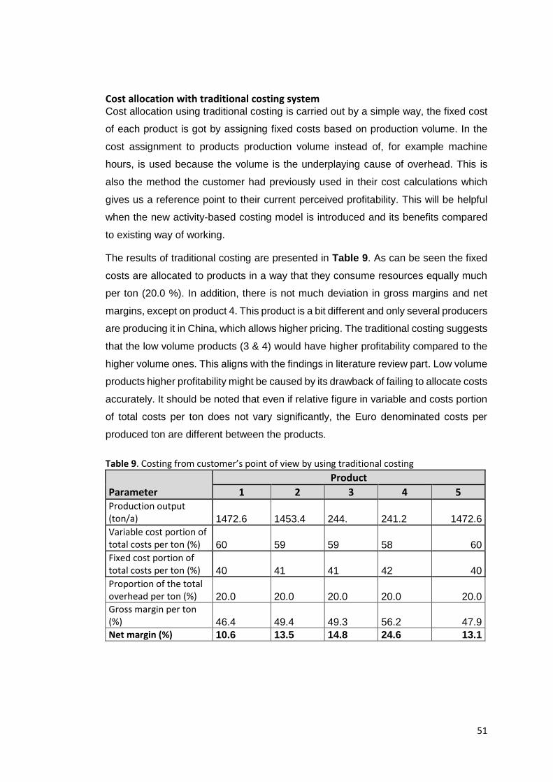
51
Cost allocation with traditional costing system Cost allocation using traditional costing is carried out by a simple way, the fixed cost
of each product is got by assigning fixed costs based on production volume. In the
cost assignment to products production volume instead of, for example machine
hours, is used because the volume is the underplaying cause of overhead. This is
also the method the customer had previously used in their cost calculations which
gives us a reference point to their current perceived profitability. This will be helpful
when the new activity-based costing model is introduced and its benefits compared
to existing way of working.
The results of traditional costing are presented in Table 9. As can be seen the fixed
costs are allocated to products in a way that they consume resources equally much
per ton (20.0 %). In addition, there is not much deviation in gross margins and net
margins, except on product 4. This product is a bit different and only several producers
are producing it in China, which allows higher pricing. The traditional costing suggests
that the low volume products (3 & 4) would have higher profitability compared to the
higher volume ones. This aligns with the findings in literature review part. Low volume
products higher profitability might be caused by its drawback of failing to allocate costs
accurately. It should be noted that even if relative figure in variable and costs portion
of total costs per ton does not vary significantly, the Euro denominated costs per
produced ton are different between the products.
Table 9. Costing from customer’s point of view by using traditional costing
Parameter
Product
1 2 3 4 5 Production output (ton/a) 1472.6 1453.4 244. 241.2 1472.6 Variable cost portion of total costs per ton (%) 60 59 59 58 60 Fixed cost portion of total costs per ton (%) 40 41 41 42 40 Proportion of the total overhead per ton (%) 20.0 20.0 20.0 20.0 20.0 Gross margin per ton (%) 46.4 49.4 49.3 56.2 47.9 Net margin (%) 10.6 13.5 14.8 24.6 13.1

52
Cost allocation with activity-based costing Determining costs by activity-based costing is essential, while the costs of activities
are not caused by – nor they hardly correlate with production output, like in previous
costs calculations they were assumed to. For example, waste handling costs per
product are only distantly in relation to production output but cannot be estimated by
traditional costing because the main driver is the amount of waste generated, which
varies among different products. As a second example, other depreciation costs
should be allocated based on machine usage time, which gives more accurate
estimation of the real usage of this resource compared to using volume for allocation
costs to the cost pools.
Implementing activity-based costing into cost allocation starts from the same starting
point than the traditional costing. What is needed besides the cost levels, however, is
the identification of main activities, their cost drivers and cost driver activity levels
which are used to allocate the costs to different products.
Activities, cost drivers, cost driver activity levels and overhead application rates are
presented in Table 10. In the model overhead items serve as activities. Cost drivers
are determined based on the root cause of the activity and the cost driver activity level
is the maximum amount cost driver can be consumed. These are calculated together
with the customer.

53
Table 10. Defining overhead application rates
Overhead item/ activity Cost driver Cost driver activity level
Indirect labour Production Machine operating hours 409500 Quality checking Batch amount 72 Engineering Batch amount 72 Warehouse Number of fluff rolls
handled 7712
Machine deprecation costs Waste handling Waste generation 220 Hammermills Machine operating hours 409500 Former Machine operating hours 409500 Calender Machine operating hours 409500 Latex binder addition Machine operating hours 409500 Oven Machine operating hours 409500 Through air dryers (second
dryer) Machine operating hours 409500
Cooling Machine operating hours 409500 Wire cleaning Latex addition 8751 Edge cutting Machine operating hours 409500 Reeling Machine operating hours 409500 Drive system Machine operating hours 409500 Cutting Number of rolls cut 150 Distribution costs Number rolls deliveries 62569 Selling, General & administrative
Tactical management labour Sold tons 4884 Operative management labour Number of workorders 72 Marketing labour Number of customers 20 Other energy costs Machine operating hours 409500 Site overhead Machine operating hours 409500 Machine maintenance and cleaning
Amount of used latex 736
Warehouse overhead raw material
Used fluff rolls 7712
Warehouse overhead finished goods
Delivered nonwoven rolls 62569
Product cutting cost Machine hours 59 Waste handling Waste generated (tons) 209 Machine set ups No. Of setups 72
In the next stage, cost driver activity rates are determined for every product, which
allows us to allocate each overhead’s expenditure to products by multiplying the
overhead application rate with cost driver activity rate. As a result, we have obtained
cost of each activity for every product. In the last stage, the total cost for every product
is calculated by summing all the allocated overhead costs of activities. The results are
seen in the Table 11 as a percentage of their total sum.

54
Table 11. Costing from customer’s point of view by using Activity-based costing
Parameter
Product
1 2 3 4 5 Production output (ton/a) 1472.6 1453.4 244.4 241.2 1472.6 Variable cost portion of total costs (%) 61 60 53 52 60 Fixed cost portion of total costs (%) 39 40 47 48 40 Fixed cost allocation increase (%) -4.0 -4.1 27.8 28.1 -1.0 Proportion of the total overhead (%) 17.5 17.5 23.4 23.4 18.1 Gross margin (%) 46.4 49.4 49.3 56.2 47.9 Net margin (%) 12.0 15.0 5.2 15.7 13.4
Cost allocation with time driven activity-based costing Compared to Activity-based costing, the model must be slightly modified in the third
and last overhead cost allocation method. Time driven activity-based costing skips
the activity-definition stage and therefore the whole need for allocate costs into
activities the company performs. In addition, in time driven activity-based costing cost
drivers are simplified to be either time, mass or area unit. This makes the model to
work simpler way assigning resource costs directly to the cost objects by using a
framework that require only two sets of estimations: the capacity cost rates and the
capacity utilization of each cost category of the department.
In the model, first, the cost of supplying resource capacities needs to be calculated.
For example, consider a process of machine set up. At first TDABC model calculates
the cost of all the resources used in process, in this case personnel and supervision,
which are the main costs. In the next stage, the total cost obtained is divided by the
capacity of the time available for the employees actually performing the process and
we get the capacity cost rate (7). Typically, this is around 80 % but varies a bit by
case.
The capacity cost rate is defined as follows:
𝐶𝑎𝑝𝑎𝑐𝑖𝑡𝑦 𝑐𝑜𝑠𝑡 𝑟𝑎𝑡𝑒
= 𝐶𝑜𝑠𝑡 𝑜𝑓 𝑐𝑎𝑝𝑎𝑐𝑖𝑡𝑦 𝑠𝑢𝑝𝑝𝑙𝑖𝑒𝑑
𝑃𝑟𝑎𝑐𝑡𝑖𝑐𝑎𝑙 𝑐𝑎𝑝𝑎𝑐𝑖𝑡𝑦 𝑜𝑓 𝑟𝑒𝑠𝑜𝑢𝑟𝑐𝑒 𝑠𝑢𝑝𝑝𝑙𝑖𝑒𝑑
(7)

55
The total amount of cost centres is significantly less than the amount of activities that
had to be defined in activity-based costing and by that it is also less time consuming.
This was done together with the managers of customer’s company. In the model, cost
inputs are absolute values but due to customer’s wish, presented (Table 12) only as
relative figures.
Table 12. Product cost by using time driven activity-based costing
Resource Cost of capacity supplied (%)
Machine deprecation 20.3
Production labour 18.7
Shipping cost 16.2
Quality labour 7.8
Management labour 6.9
Other energy costs 6.5
Site overhead 5.4
Production lost 4.1
Engineering labour 3.5
Additional delivery costs for international shipments 2.2
Additional packaging 2.2
Warehousing costs raw material 1.6
Warehouse cost finished goods 1.6
Warehousing labour 1.6
Cutting machine usage (deprecation) 0.8
Waste handling cost 0.6
In the next stage, theoretical and practical capacities are estimated. As found out in
the literature review, the aim here is not to reach to full precision, but instead to get
the general alignment. To estimate the practical capacity, the quantity of resources
(personnel or equipment) is identified. For example, in this, production labour practical
capacity is calculated as follows: number of production workers required in operations
that work the equal time the machine is running plus required time for breaks, trainings
and considering that not all the paid time is productive work. This leaves the practical
capacity to be 70 % of the theoretical capacity. This ratio differs from 70 % (personnel)
to 100 % (machinery). After calculating the practical capacity, the capacity cost rate
can be calculated for all the resources.
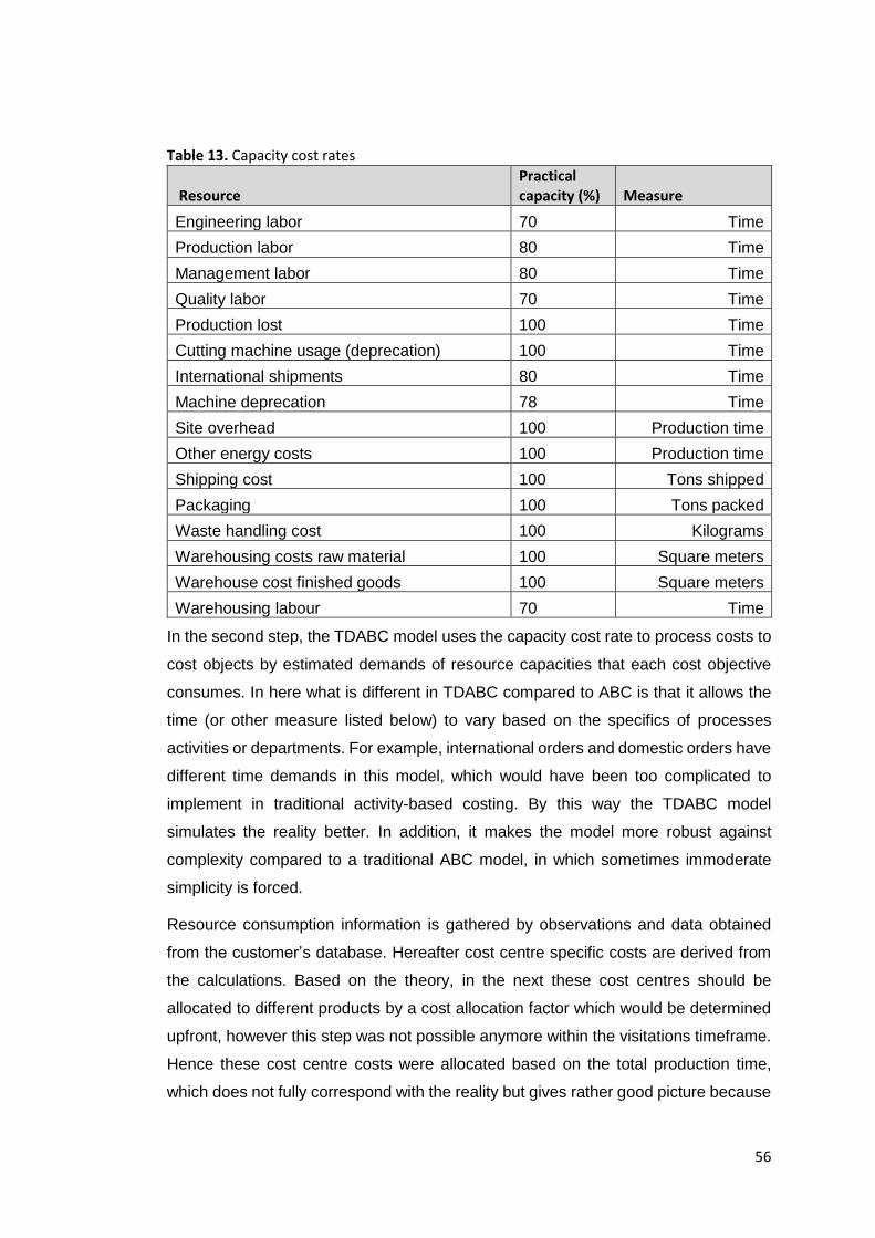
56
Table 13. Capacity cost rates
Resource Practical capacity (%) Measure
Engineering labor 70 Time
Production labor 80 Time
Management labor 80 Time
Quality labor 70 Time
Production lost 100 Time
Cutting machine usage (deprecation) 100 Time
International shipments 80 Time
Machine deprecation 78 Time
Site overhead 100 Production time
Other energy costs 100 Production time
Shipping cost 100 Tons shipped
Packaging 100 Tons packed
Waste handling cost 100 Kilograms
Warehousing costs raw material 100 Square meters
Warehouse cost finished goods 100 Square meters
Warehousing labour 70 Time
In the second step, the TDABC model uses the capacity cost rate to process costs to
cost objects by estimated demands of resource capacities that each cost objective
consumes. In here what is different in TDABC compared to ABC is that it allows the
time (or other measure listed below) to vary based on the specifics of processes
activities or departments. For example, international orders and domestic orders have
different time demands in this model, which would have been too complicated to
implement in traditional activity-based costing. By this way the TDABC model
simulates the reality better. In addition, it makes the model more robust against
complexity compared to a traditional ABC model, in which sometimes immoderate
simplicity is forced.
Resource consumption information is gathered by observations and data obtained
from the customer’s database. Hereafter cost centre specific costs are derived from
the calculations. Based on the theory, in the next these cost centres should be
allocated to different products by a cost allocation factor which would be determined
upfront, however this step was not possible anymore within the visitations timeframe.
Hence these cost centre costs were allocated based on the total production time,
which does not fully correspond with the reality but gives rather good picture because
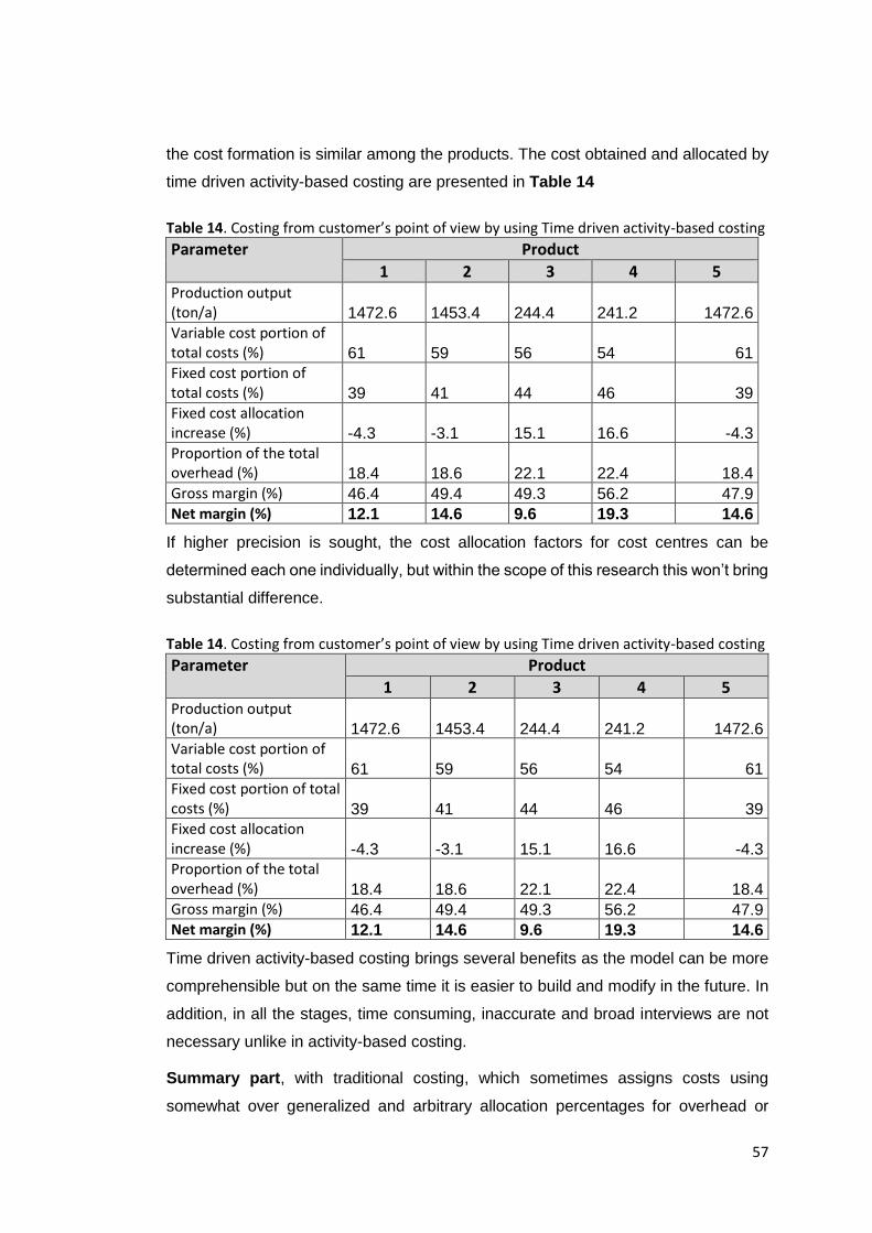
57
the cost formation is similar among the products. The cost obtained and allocated by
time driven activity-based costing are presented in Table 14
Table 14. Costing from customer’s point of view by using Time driven activity-based costing
Parameter Product
1 2 3 4 5 Production output (ton/a) 1472.6 1453.4 244.4 241.2 1472.6 Variable cost portion of total costs (%) 61 59 56 54 61 Fixed cost portion of total costs (%) 39 41 44 46 39 Fixed cost allocation increase (%) -4.3 -3.1 15.1 16.6 -4.3 Proportion of the total overhead (%) 18.4 18.6 22.1 22.4 18.4 Gross margin (%) 46.4 49.4 49.3 56.2 47.9 Net margin (%) 12.1 14.6 9.6 19.3 14.6
If higher precision is sought, the cost allocation factors for cost centres can be
determined each one individually, but within the scope of this research this won’t bring
substantial difference.
Table 14. Costing from customer’s point of view by using Time driven activity-based costing
Parameter Product
1 2 3 4 5 Production output (ton/a) 1472.6 1453.4 244.4 241.2 1472.6 Variable cost portion of total costs (%) 61 59 56 54 61 Fixed cost portion of total costs (%) 39 41 44 46 39 Fixed cost allocation increase (%) -4.3 -3.1 15.1 16.6 -4.3 Proportion of the total overhead (%) 18.4 18.6 22.1 22.4 18.4 Gross margin (%) 46.4 49.4 49.3 56.2 47.9 Net margin (%) 12.1 14.6 9.6 19.3 14.6
Time driven activity-based costing brings several benefits as the model can be more
comprehensible but on the same time it is easier to build and modify in the future. In
addition, in all the stages, time consuming, inaccurate and broad interviews are not
necessary unlike in activity-based costing.
Summary part, with traditional costing, which sometimes assigns costs using
somewhat over generalized and arbitrary allocation percentages for overhead or

58
indirect costs, result often unreal and misleading estimates. This is particularly
harmful if the production of products has different characteristics. In the case
company, the major differences in costs are caused by different product compositions
of raw material and the latex binder that is added. In addition, the machine speed and
production output have a big impact to profitability. When taking these into account,
the real costs differs quite lot between products. This can be seen in the Figure 20
where overhead costs per ton are presented by product. In traditional costing all the
products have the equal amount of fixed costs allocated to them per ton. In the
activity-based costing the high-volume products, the same product that consumer less
latex binder and have higher machine speed (products 1, 2 & 5) have relatively lower
overhead costs compared to the special products 3 and 4. Finally, the time driven
activity-based costing results are something between the traditional costing and
activity-based costing. Like activity-based costing, the time driven activity-based
costing is allocates relatively speaking less costs to the products 1, 2 & 5 and more
to the products 3 & 5, although the difference between these product groups is not as
significant as in activity-based costing.
Figure 20. Proportion of the total overhead per ton by product with different costing systems
Figure 21 presents the model’s results by breaking down variable and fixed costs of
products by the costing systems used. The results do not vary significantly between
20,0 % 20,0 % 20,0 % 20,0 % 20,0 %
17,5 % 17,5 %
23,4 % 23,4 %
18,1 %
18,4 % 18,6 %
22,1 % 22,4 %
18,4 %
0%
5%
10%
15%
20%
25%
30%
Product 1 Product 2 Product 3 Product 4 Product 5
Traditional costing Activity-based costing
Time driven activity-based costing

59
the cost systems in the higher volume products 1, 2 & 5. The difference is from -3.4 %
to -4.3 % (Table 15), which should be still noted as this multiplied with the total fixed
cost of a product equals to 30 – 50 €/t. The more significant difference is in the
products 3 and 4 where the fixed cost difference of the three costing systems result
in +15.1 % to +28.1 % increase in the fixed costs compared to traditional costing. This
transfers roughly to 100 – 250 €/t.
Figure 21. Cost breakdown of products to variable and fixed cost by costing system
Table 15 presents the fixed cost allocation increase/decrease compared to traditional
costing, system that the customer used. This also supports the idea that activity-
based costing and time driven activity-based costing are better at allocating fixed
40,1 % 39,1 % 39,0 % 41,4 % 40,4 % 40,7 % 40,5 %46,5 % 43,9 % 41,9 %
48,0 % 45,7 %40,1 % 39,8 % 39,0 %
59,9 % 60,9 % 61,0 % 58,6 % 59,6 % 59,3 % 59,5 %53,5 % 56,1 % 58,1 %
52,0 % 54,3 %59,9 % 60,2 % 61,0 %
0 %
20 %
40 %
60 %
80 %
100 %
Trad
itio
nal
co
stin
g
Act
ivit
y-b
ase
d c
ost
ing
Tim
e d
rive
n a
ctiv
ity-
bas
ed c
ost
ing
Trad
itio
nal
co
stin
g
Act
ivit
y-b
ase
d c
ost
ing
Tim
e d
rive
n a
ctiv
ity-
bas
ed c
ost
ing
Trad
itio
nal
co
stin
g
Act
ivit
y-b
ase
d c
ost
ing
Tim
e d
rive
n a
ctiv
ity-
bas
ed c
ost
ing
Trad
itio
nal
co
stin
g
Act
ivit
y-b
ase
d c
ost
ing
Tim
e d
rive
n a
ctiv
ity-
bas
ed c
ost
ing
Trad
itio
nal
co
stin
g
Act
ivit
y-b
ase
d c
ost
ing
Tim
e d
rive
n a
ctiv
ity-
bas
ed c
ost
ing
Product 1 Product 2 Product 3 Product 4 Product 5
Fixed costs Variable costs
60
costs. In this case, the major factors are the production volume’s influence, latex
binder addition and machine speed. It is a bit unclear why the activity-based costing
and time driven-activity based costing give different values for product 5 as in other
high-volume products they are quite closely aligned. Also, it is worth noting how big
of a difference traditional costing gives as a result for products 3 and 4 compared with
the activity-based costing and time driven activity-based costing.
Table 15. Fixed cost allocation increase/decrease compared to traditional costing
Product
1 2 3 4 5 Production output (ton/a) 1472.6 1453.4 244.4 241.2 1472.6
Activity-based costing (%) -4.0 -4.1 +27.8 +28.1 -1.0 Time driven activity-based costing (%) -4.3 -3.1 +15.1 +16.6 -4.3
If selling prices are considered as well, we can see that profitability among products
varies too when using different costing systems (Figure 22). This is especially true
for the products 3 and 4. With the traditional costing, it seems that the product 4 is
much more profitable than the others with an 24.6 % net profit compared to other
products 10 – 15 % profit margin.
Figure 22. Net margin by product with different costing systems
10,6 %
13,5 % 14,8 %
24,6 %
13,1 %12,0 %
15,0 %
5,2 %
15,7 % 13,4 %12,1 % 14,6 %
9,6 %
19,3 %
14,6 %
0%
5%
10%
15%
20%
25%
30%
Product 1 Product 2 Product 3 Product 4 Product 5
Traditional costing Activity-based costing
Time driven activity-based costing
61
In addition, the results suggest that those products that can be easily produced by
other manufacturing technologies than latex bonded airlaid have lower profitability
levels in traditional costing. This is most likely due to higher competition. However,
the products 3 and 4 that are considered as special products and can be only
produced with airlaid production technique have lower profitability when calculated by
activity-based costing and time driven activity-based costing although the traditional
costing would have suggested otherwise.
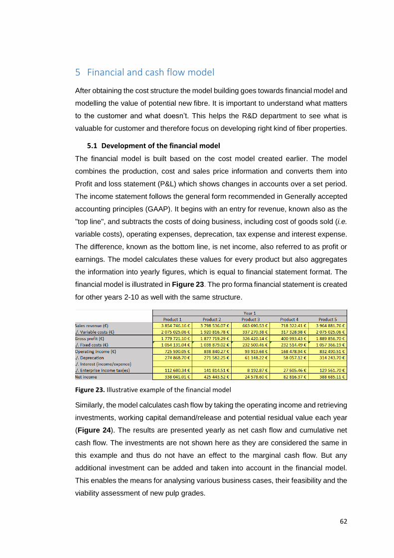
62
5 Financial and cash flow model
After obtaining the cost structure the model building goes towards financial model and
modelling the value of potential new fibre. It is important to understand what matters
to the customer and what doesn’t. This helps the R&D department to see what is
valuable for customer and therefore focus on developing right kind of fiber properties.
5.1 Development of the financial model
The financial model is built based on the cost model created earlier. The model
combines the production, cost and sales price information and converts them into
Profit and loss statement (P&L) which shows changes in accounts over a set period.
The income statement follows the general form recommended in Generally accepted
accounting principles (GAAP). It begins with an entry for revenue, known also as the
"top line", and subtracts the costs of doing business, including cost of goods sold (i.e.
variable costs), operating expenses, deprecation, tax expense and interest expense.
The difference, known as the bottom line, is net income, also referred to as profit or
earnings. The model calculates these values for every product but also aggregates
the information into yearly figures, which is equal to financial statement format. The
financial model is illustrated in Figure 23. The pro forma financial statement is created
for other years 2-10 as well with the same structure.
Figure 23. Illustrative example of the financial model
Similarly, the model calculates cash flow by taking the operating income and retrieving
investments, working capital demand/release and potential residual value each year
(Figure 24). The results are presented yearly as net cash flow and cumulative net
cash flow. The investments are not shown here as they are considered the same in
this example and thus do not have an effect to the marginal cash flow. But any
additional investment can be added and taken into account in the financial model.
This enables the means for analysing various business cases, their feasibility and the
viability assessment of new pulp grades.

63
Figure 24. Illustrative example of the cash flow model
Working capital in the cash flow model is calculated by including operating activities
that represents only the core accounts that make up working capital in day-to-day
operations. Working capital operating activities consist of account payables (8),
accounts receivables (9) and production process (10) which are calculated by using
specific working capital cycles. In reality the working capital would also consist of cash
and short-term financing, but as we are only interested in marginal cash flow and
assuming those items are same in status quo and new production, these does not
have to be taken into account.
𝐴𝑐𝑐𝑜𝑢𝑛𝑡𝑠 𝑝𝑎𝑦𝑎𝑏𝑙𝑒𝑠
=𝐶𝑜𝑠𝑡 𝑜𝑓 𝑔𝑜𝑜𝑑𝑠 𝑠𝑜𝑙𝑑 ∗ 𝐴𝑐𝑐𝑜𝑢𝑛𝑡𝑠 𝑝𝑎𝑦𝑎𝑏𝑙𝑒 𝑑𝑎𝑦𝑠
365
(8)
𝐴𝑐𝑐𝑜𝑢𝑛𝑡𝑠 𝑟𝑒𝑐𝑒𝑖𝑣𝑎𝑏𝑙𝑒𝑠
=𝐴𝑛𝑛𝑢𝑎𝑙 𝑐𝑟𝑒𝑑𝑖𝑡 𝑠𝑎𝑙𝑒𝑠 ∗ 𝐴𝑐𝑐𝑜𝑢𝑛𝑡𝑠 𝑟𝑒𝑐𝑒𝑖𝑣𝑎𝑏𝑙𝑒 𝑑𝑎𝑦𝑠
365
(9)
Production process is the sum of working capital bound to raw materials (11), work in
progress (12), finished goods (13) and fixed costs (15). It is worth noting that in
finished goods, the net profit is not included in the working capital and therefore does
not have to be financed. In addition, it is important to remember to take into account
the fixed costs as well as they play rather big part as the turnover rate is relatively low.
𝑃𝑟𝑜𝑑𝑢𝑐𝑡𝑖𝑜𝑛 𝑝𝑟𝑜𝑐𝑒𝑠𝑠= 𝑅𝑎𝑤 𝑚𝑎𝑡𝑒𝑟𝑖𝑎𝑙 + 𝑊𝑜𝑟𝑘 𝑖𝑛 𝑝𝑟𝑜𝑐𝑒𝑠𝑠+ 𝐹𝑖𝑛𝑖𝑠ℎ𝑒𝑑 𝑔𝑜𝑜𝑑𝑠 + 𝐹𝑖𝑥𝑒𝑑 𝑐𝑜𝑠𝑡
(10)
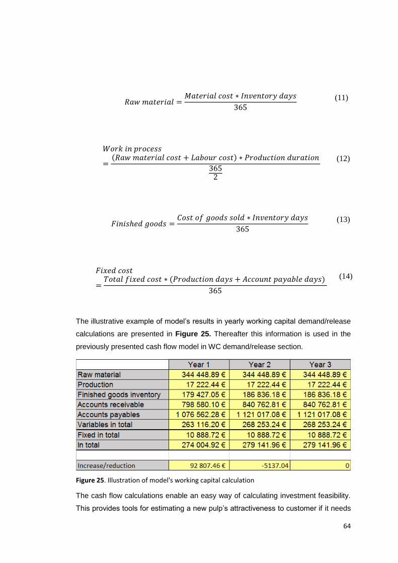
64
𝑅𝑎𝑤 𝑚𝑎𝑡𝑒𝑟𝑖𝑎𝑙 =𝑀𝑎𝑡𝑒𝑟𝑖𝑎𝑙 𝑐𝑜𝑠𝑡 ∗ 𝐼𝑛𝑣𝑒𝑛𝑡𝑜𝑟𝑦 𝑑𝑎𝑦𝑠
365
(11)
𝑊𝑜𝑟𝑘 𝑖𝑛 𝑝𝑟𝑜𝑐𝑒𝑠𝑠
=(𝑅𝑎𝑤 𝑚𝑎𝑡𝑒𝑟𝑖𝑎𝑙 𝑐𝑜𝑠𝑡 + 𝐿𝑎𝑏𝑜𝑢𝑟 𝑐𝑜𝑠𝑡) ∗ 𝑃𝑟𝑜𝑑𝑢𝑐𝑡𝑖𝑜𝑛 𝑑𝑢𝑟𝑎𝑡𝑖𝑜𝑛
3652
(12)
𝐹𝑖𝑛𝑖𝑠ℎ𝑒𝑑 𝑔𝑜𝑜𝑑𝑠 =𝐶𝑜𝑠𝑡 𝑜𝑓 𝑔𝑜𝑜𝑑𝑠 𝑠𝑜𝑙𝑑 ∗ 𝐼𝑛𝑣𝑒𝑛𝑡𝑜𝑟𝑦 𝑑𝑎𝑦𝑠
365
(13)
𝐹𝑖𝑥𝑒𝑑 𝑐𝑜𝑠𝑡
=𝑇𝑜𝑡𝑎𝑙 𝑓𝑖𝑥𝑒𝑑 𝑐𝑜𝑠𝑡 ∗ (𝑃𝑟𝑜𝑑𝑢𝑐𝑡𝑖𝑜𝑛 𝑑𝑎𝑦𝑠 + 𝐴𝑐𝑐𝑜𝑢𝑛𝑡 𝑝𝑎𝑦𝑎𝑏𝑙𝑒 𝑑𝑎𝑦𝑠)
365
(14)
The illustrative example of model’s results in yearly working capital demand/release
calculations are presented in Figure 25. Thereafter this information is used in the
previously presented cash flow model in WC demand/release section.
Figure 25. Illustration of model's working capital calculation
The cash flow calculations enable an easy way of calculating investment feasibility.
This provides tools for estimating a new pulp’s attractiveness to customer if it needs
65
modifications to their existing line. In addition, it helps sales team and technical
customer service team to communicate the new pulp’s benefits to customers.
After calculating cash flow, all the financial metrics can be calculated. By using values
the cost model and financial model result, the model calculates Net present value,
Internal rate of return, Pay-back time, Economic value addition, Return on capital
employed and Return on assets. In addition, EBITDA and EBITDA-% is calculated.
These are given for the customer as a guiding tool. In addition, it helps them to
understand the new pulp grades effects to their profitability.
All the values are calculated for one or several kinds of pulps and the results can be
compared with each other. The financial model has two functions. Firstly, it can be
used as a sales promotion tool for evidencing the benefits of the company’s offering,
which is different compared to the general pulp in the markets. Secondly it can be
used for developing new kind of pulp and quantifying the potential monetary value of
the novel pulp developed. For example, if a kind of pulp that requires less latex binder
addition is developed, what would be its value for the customer and subsequently its
potential selling price.
5.2 Introducing the financial model case study
In the case study the financial model and cash flow model and brought to an actual
business case. In the first phase of financial modelling, current operating income and
pro operating incomes for next nine years are calculated. After this the current cash
flow and similarly pro forma cash flows are calculated for status quo and “new
production”. The status quo refers to the current state of things and new production
refers to a situation where modifications to operations have been made. The
modification can be any sort but just to give some idea, it can be for example a new
pulp type which has different price, properties, machine settings, etc. The result is a
marginal cash flow that gives a monetary value for the modifications case-by-case. In
the next section we go through an example of this.
In the status quo, the three hammermills (Figure 16) that defibrillize pulp rolls to their
own formers are infeed with two fluff pulp grades with a settings shown in Table 16.
Fluff pulp grade is used in the upper and bottom layer of the nonwoven and fluff pulp
grade Y is used in middle layer. In the New production the upper and bottom layers’
the fluff pulp grade X is replaced with “new fluff pulp grade” The new fluff pulp grade
differences from the regular fluff pulp grade X by better formation, even web, lower
energy usage in hammer mill and lower latex binder requirement. On the other hand,

66
the new fluff pulp grade is more expensive compared to the other pulp grades the
customer used in the status quo production.
Table 16. Fluff pulp grades used before and after the modifications
Hammermill Product layer Status quo New production Hammermill/former 1 Upper Fluff pulp grade X New fluff pulp
grade
Hammermill/former 2 Middle Fluff pulp grade Y Fluff pulp grade Y Hammermill/former 3 Bottom Fluff pulp grade X New fluff pulp
grade
The modifications from status quo to new production in this example did not require
any investment. However, the cash flow model can take this into account. In addition,
the production rate and basis weight were not changed even though the new fluff pulp
grade would allow this due the even web and lower latex binder usage. Higher
production rate and lower basis weight would have required modifications to the
production line and therefore the hypothesis could not be verified.
The case study uses the previously introduce production model, financial statement
model and cash flow model. So firstly, the parameters are updated. In practice, this
means adding a new pulp grade to “VlookUp-table” from which the production model
retrieves the data. In addition, the production model is told to use this new pulp grade
in the New production and for example switch the latex binder usage amount. In this
case the latex binder reduction was estimated to be 20 % lesser than in status quo.
However, this can vary, and the final figure depends on customer’s final preferences.
After this the financial model calculates profitability for before and after situations and
marginal profitability is calculated using by subtracting new production profitability
from status quo production (15) and the future cash flows are discounted to present
value by using equation (16. This will result in case-by-case comparable figures. In
addition, it will provide profitability results that only take into account the increased
profitability. This is important because then the current already existing profitability
can be excluded, and the real profitability improvement can be determined.
𝑀𝑎𝑟𝑔𝑖𝑛𝑎𝑙 𝐶𝐹 = 𝑆𝑡𝑎𝑡𝑢𝑠 𝑞𝑢𝑜 𝐶𝐹 − 𝑁𝑒𝑤 𝑝𝑟𝑜𝑑𝑢𝑐𝑡𝑖𝑜𝑛 𝐶𝐹 (15)
Where, CF refers to Cash flow

67
𝑀𝑎𝑟𝑔𝑖𝑛𝑎𝑙 𝐷𝐶𝐹 =𝑀𝑎𝑟𝑔𝑖𝑛𝑎𝑙 𝐶𝐹
(1 + 𝑟)2 (16)
Where, DCF = Discounted cash flow r = Discount rate (WACC) The results are presented in Figure 26. Compared to last period’s cumulative
discounted net cash flow, the new production is 42.9 % higher than status quo and
the first year’s marginal cash flow is 7.4 % higher. This rate decreases in later periods
as the time value of the cash flows reduces the impact. The discount rate used (in this
case the weighted average cost of capital) was calculated to be 9.4 %.
Figure 26. Cumulative marginal discounted cash flow increase
What it comes to fixed costs, there were three alternatives for cost modelling: the
traditional costing, activity-based costing and time driven activity-based costing. Only
one is going to be implemented here and as discussed in the Chapter 4, the most
accurate one proved to be activity-based costing. Therefore, the financial model uses
this to provide the cost information in product level. The new production’s selling price
is set to stay the same as in status quo although it could be higher than the status
quo because the lower latex binder amount increases the product’s hand feel softness.
5.3 Sensitivity analysis
To analyse how different values of an independent variable impact a particular
dependent variable a sensitivity analysis was built in the model financial and cash
42,9 %
0%
5%
10%
15%
20%
25%
30%
35%
40%
45%
50%
0 1 2 3 4 5 6 7 8 9 10
Period
Marginal cumulative discounted cash flow increase

68
flow model. The model is used within specific boundaries that depend on several input
variables. A set of variables were chosen that were defined to affect most on
profitability. The outcome in the other hand was chosen to be cumulative cash flow
and new fluff pulp price.
Figure 27 presents the cash flow model’s sensitivity results over cumulative net cash
flow which is calculated by equation (15)(16). Based on the results we can categorise
the variables into three main groups based on slope of the curve. There are variables
that are critical, important and small cash flow increase/decrease potential. Selling
price and production output belong to the critical group. If selling price could be
increased 20 % the cumulative net cash flow would increase 95.1 %, so nearly double.
Following the same logic, if production output could be increased by 20 %, the
cumulative net cash flow would increase 45.1 %. Obviously that high increase,
especially in the selling price is most likely not possible, but it tells what fundamentally
affects to profitability the most. On the other hand, the selling price increase is not
totally impossible as the selling price is per tons, which might get higher if basis weight
could be decreased. The outcome of this can be obtained by firstly following the
production rate slope (same or decreased) and then the selling price slope (same or
increased). Their net difference would be the cumulative net cash flow gain.
Pulp price, fixed costs, latex binder price and latex binder amount belong to the
important group. Their impact to the net cumulative cash flow is significant but not as
high as the critical group’s. However, it should be noted that in many cases influencing
these variables in operational level might be easier than those of in critical group.
The last group contains variables than have an impact to the cash flow, but not as
significant as the variables in the two other groups. Namely they are hammermill
energy consumption, energy cost (electricity), maintenance, formation waste and
energy cost (heating). These variables importance should not be undermined as the
final additional profitability can be made by making sure these are well taken care of.
Due to the customer’s wish, the energy cost was chosen as a variable instead if
energy consumption as they though the energy price is on an upward pressure in
China.

69
Figure 27. Sensitivity analysis: Cumulative net cash flow increase/decrease
The sensitivity model can be used in two ways. Firstly, it helps the research and
development team to identify in which areas they should focus on to maximise the
customer’s value. On the same time, it clarifies the pulp characteristics needed and
key information for calculating the potential selling price. Secondly, it can be used as
a scenario analysis. For example, if the energy cost or fluff pulp price is due to
increase in the future, the sensitivity model helps to identify their impact. This helps
the customer and the whole value chain to focus on key risk mitigation factors and
focus on the right things in the future.
-100%
-80%
-60%
-40%
-20%
0%
20%
40%
60%
80%
100%
-30 % -20 % -10 % 0 % +10 % +20 % +30 %
Cu
mu
lati
ve n
et c
ash
flo
w c
han
ge
Change to valueProduction output Selling pricePulp price Latex amountLatex price MaintenanceHammermill energy consumption Formation wasteEnergy cost (electricity) Energy cost (heating)Fixed costs

70
6 Value creation at UPM-Kymmene
6.1 Simulated new fluff pulp price
The new selling price represents the novel pulp’s selling price based on its new
characteristics. For example, if the latex-binder infeed amount can be reduced by X %
due to novel fibres, what could be its selling price if the benefits are shared between
the pulp producer and other partners in the value chain. In this example it is thought
that 25 % of the benefits are allocated to the new fluff pulp price (Equation (17). The
exact value of this would be determined in the price negotiations case-by-case. The
benefits are simulated in the financial model based on the new variables by using the
following formula:
𝑁𝑒𝑤 𝑓𝑙𝑢𝑓𝑓 𝑝𝑢𝑙𝑝 𝑝𝑟𝑖𝑐𝑒 =𝑀𝑎𝑟𝑔𝑖𝑛𝑎𝑙 𝐶𝐹
𝐹𝑙𝑢𝑓𝑓 𝑝𝑢𝑙𝑝 𝑐𝑜𝑛𝑠𝑢𝑚𝑝𝑡𝑖𝑜𝑛∗ 𝑋 (17)
Where, CF = Cash flow X = Fluff pulp producers share of the improvement gains (25 %) The new fluff pulp prices in different simulations are presented in Figure 28. The
results resemble marginal cash flow results with the variable importance order, but
naturally the model gives different values as it is divided by fluff pulp consumption and
multiplied by fluff pulp producer’s share of the improvement gains. Again, variables
are categorised into three main group: critical, important and small selling price
increase/decrease potential. The critical group consists of nonwoven selling price and
production output. For example, if by the new fluff pulp the nonwoven selling price
could be increased by 10 %, the cash flow increase of this would allow 9.8 % increase
to fluff pulp price. Following the same logic, if production output increases by 10 %,
the new fluff pulp price could be 4.3 % higher.
Important group consist of fixed costs, latex binder price and added latex binder
amount. Their impact to the price increase/decrease is significant but not as high as
the critical group’s. Their potential increase to selling price range from + 3.2 % to
+ 8.2 % if variables are changed to value + 30 %. Especially on the fixed cost and
latex binder addition this kind of change is possible. However, especially on fixed cost
saving it might be hard in real situation to negotiate price increase. Example of this

71
kind of case might be that if some process step could be totally skipped due to an
innovation, then the customer might be willing to pay extra.
The last group contains variables than have a small impact to potential selling price
increase/decrease. Variable belonging to this category are hammermill energy
consumption, energy cost (electricity), maintenance, formation waste and energy cost
(heating). Their positive impact ranges from 0.3 % to 2.4 % increase in the potential
new selling price.
Figure 28. Sensitivity analysis: New fluff pulp price increase/decrease
It should be noted that there might be also some other qualitative variables that bring
value to the customer that cannot be modelled in the financial and cash flow model.
For example, especially in China customers value specialized technical customer
service but also long-lasting customer relationships are known to be valuable for pulp
customers. In addition, reliability of supply, pulp’s purity, low amount of dust, low static
electricity build-up, standards and certification and product safety bring value to the
-20,0 %
-17,5 %
-15,0 %
-12,5 %
-10,0 %
-7,5 %
-5,0 %
-2,5 %
0,0 %
2,5 %
5,0 %
7,5 %
10,0 %
12,5 %
15,0 %
17,5 %
20,0 %
-30 % -20 % -10 % 0 % +10 % +20 % +30 %
New
flu
ff p
ulp
pri
ce c
han
ge
Change to valueProduction output Selling price
Latex amount Latex price
Maintenance Hammermill energy consumption
Formation waste Energy cost (electricity)
Energy cost (heating) Fixed costs

72
customer but cannot be directly modelled by changing any variable in the models.
However, indirectly those can be calculated by studying their cause-and-effect
relationship. The lack of reliability of supply would mean that the customer must
increase their inventory buffers meaning higher working capital requirement. This is a
cost for the customer which can be entered as an input and the model calculates the
value for this. The value of product safety, standards, certifications and forest
schemes could be monetarized by changing the selling price variable as usually those
products price is higher, and demand is more stable. Lesser amount of dust’s value
can be simulated by changing the yield parameter in the model. However, giving an
exact value for these qualitative factors is impossible and not even necessary.
6.2 Value creation to R&D and target costing
After calculating what brings value to the customer and what could the selling price,
we can determine the target cost (allowable costs) of new products as in Figure 15.
This can be calculated by subtracting desired profit from market price as in Equation
(18). Target cost refers to the same as “Total Cost” in Table 3 but in the different case.
𝑇𝑎𝑟𝑔𝑒𝑡 𝑐𝑜𝑠𝑡 = 𝑀𝑎𝑟𝑘𝑒𝑡 𝑝𝑟𝑖𝑐𝑒 − 𝐷𝑒𝑠𝑖𝑟𝑒𝑑 𝑝𝑟𝑜𝑓𝑖𝑡 (18)
Where,
Desired profit = Market price * target profit margin
By assuming the target profit margin is 20 %, we can calculate the target cost for each
sensitivity variable. The results are presented in Figure 29. Naturally, as the selling
price and production output were the most important cash flow variables, so are they
in target costs. The results also show quite clear improvement potential in latex binder
addition and fixed cost. How the results should be interpreted is for example that if
latex binder addition could be reduced by 10 % the cost of own production could be
1.2 % higher and would still be beneficial for both parties. Naturally, if the sum of
development and production costs are lower than 1.2 %, the value chain would make
more money, but the 1.2 % is the feasibility threshold. The reason why latex binder
price has a bigger effect compared to latex binder addition is that the latter one has
an effect to the production rate and therefore if it decreases the total amount of tons
sold decreases. This leads to decrease in cash flow and its impact is even bigger than
the drying energy cost savings.
Selling price (€/t) increase for customer could be achieved by reducing the airlaid
nonwovens’ basis weight (€/m2) and on the same time keeping the production output

73
in tons the same. Even a slight change to this would be highly beneficial. There is not
an own sensitivity parameter for basis weight increase/decrease but adjusted selling
price can be used for this. In the similar way the effect of increased absorption
capacity can be estimated.
Figure 29. Allowable increase in costs in relation to fluff pulp production cost
Quite significant potential is also on finding ways to decrease fixed cost. The total cost
of a pulp grade that decreases the customer’s fixed costs by 10 % can be 2.6 % more
expensive. In practice this could mean getting rid of a process step for example one
of the latex binder addition steps. The exact cost saving of is not known but based on
the potential it could be something interesting to investigate in the future. Reducing
customer’s formation waste would allow some but only low-cost actions in pulp
production. If the customer’s waste could be reduced by 30 % the pulp production
cost increase must not be higher than 1 %. Tackling this issue in reality might prove
to be challenging but one key element in formation waste generation is the amount of
fibre bundles in fluff pulp and consistent quality. Surprisingly, energy costs and
-6%
-5%
-4%
-3%
-2%
-1%
0%
1%
2%
3%
4%
5%
6%
-30 % -20 % -10 % 0 % +10 % +20 % +30 %
Allo
wab
le c
ost
incr
ease
/dec
reas
e
Change to value
Production output Selling price
Latex amount Latex price
Maintenance Hammermill energy consumption
Formation waste Energy cost (electricity)
Energy cost (heating) Fixed costs

74
hammermill energy consumption proved to be less important as anticipated.
Decreasing customers drying energy costs by 30 % would allow 1.1 % cost increase
in pulp production. However, it should be noted that the energy consumption is much
related to latex-binder addition. Therefore, the latex-binder addition amount is so
important as it reduces the amount of latex binder. Latex binder’s solid content is 50 %
and when it’s amount is reduced it less drying is needed to reach to nonwoven’s end
consistency. As hammermill energy consumption plays a minor direct role in the cost
saving potential. What matters in hammermill however is the defibrillization.
Consistent quality and minimal fibre bundles allow lower basis weight, higher
production rate and potentially higher selling price due to higher quality in terms of
better surface softness. Reducing maintenance need for customer could be also one
potential area where pulp R&D could focus on. This is true especially if solutions could
be found on static electricity build-up. Currently the moisture content is high in the
production hall which accelerates corrosion. This results in higher maintenance costs.
The potential effect of this could be even higher as the model does not take into
account the fact that the machines worn out sooner. Thus, the depreciation schedule
should be modified accordingly. However, this is hard to model with good enough
precision. The detailed allowable increase in costs by variable can be found in
Appendix 3.
There are also several benefits than cannot be modelled in a financial and cash flow
model. Therefore, the customers willingness to pay for new fluff pulp’s properties it
might be still that they value it more and in case of overcapacity in the markets it is
easier to sell and keep pulp mills operating rate high. Even this would bring value for
the pulp producer and those ideas the R&D sector should also consider. For example,
the R&D sector can support technical customer service on problem solving. This helps
to build reliable business partnership which the Chinese customer appreciate but are
not willing to pay more. In addition, opacity and environmental performance and
image might be that kind of property. Especially certified production plays an
important role.
When thinking about the overall cost structure and how certain modifications to fluff
pulp might affect to the total increase/decrease in total production cost, the Table 3
is a good reference point. It can be used to get the first estimations of if the target cost
can be reached or not.

75
7 Conclusion
This chapter recaps the objectives and research questions of this thesis, summarizes,
and discusses the main findings. In addition, this chapter will analyse the validity and
reliability of this research and finally discuss the further research opportunities from
the area and results. This thesis contributes to supply chain management and supply
chain cost management. In these fields especially to financial value chain which is the
value chain perspective and the logistic perspective is limited out of the scope.
This thesis had two main objectives.
1) To develop an approach for understanding fluff pulp customers’ operations and cost structure in Mainland China.
2) To examine pulp R&D value creation potential in fluff pulp value chain and determine new fluff pulp prices for several variables.
From those objectives the main research question, “How Cost Management methods
and financial modelling can be utilized to support pulp R&D function in novel fibre
development for a customer in fluff pulp value chain in Mainland China?”, was derived
and split into three sub-questions.
A first sub-research question, “Which of the Cost Management methods is most
applicable for creating a model that quantifies the current cost structure of a customer
in Mainland China?” was derived from the first objective. This research question is
addressed especially in sections 3 and 4.
Sub-questions two and three are related with the second objective.
Sub-question two, “In which way the model needs to be developed to best obtain
increased customers’ value of a new pulp grade and new fibre properties?”, is
addressed in the end of section three and in section five. These sections also discuss
what is the best financial measure to demonstrate the benefits and what matters the
most for the customer. Subsequently, the research gives direction on where to focus
on fluff pulp development activities.
Finally, the sub-question three, “What is the new selling price and allowable additional
costs of a potential new type of fibre sold to a customer in Mainland China?”, is
addressed in section 6 which further utilises the cash flow model and makes an
estimation of potential selling prices based on the allocation method.

76
7.1 Theoretical implications
This thesis introduces the cost model, financial model and cash flow model. The cost
model was designed for analysing the cost structure of current operations and
comparing three alternative costing methods: traditional costing, activity-based
costing and time driven activity-based costing. These were selected by either
mapping out the most potential ones in literature as in activity-based costing’s and
time driven activity based costing’s case or using the current costing method that the
customer used - traditional costing. Analysing the cost structure by this way gives
reliable information about the cost structure in Mainland China. This was important as
the different costing methods deliver different results and in worst case, the current
methods used might steer to focus on wrong products that were not as profitable as
imagined, both in customer’s decision making and pulp R&D’s side. Therefore,
validating research theories with a case study was important.
The results in fixed costs align with the previous research, the traditional costing leads
to overly allocated fixed costs to high volume products and similarly too less fixed
costs to low volume products. In the high volume products, the allocated fixed cost
was around 4 % lower in terms of €/ton when comparing traditional costing to activity-
based costing or time driven activity-based costing. In the low volume products, the
fixed cost was roughly 28 % higher when comparing activity based costing to
traditional costing and 15 -16 % higher when comparing it to time driven activity-based
costing (Table 15). The reason why activity-based costing and time driven activity-
based costing delivered slightly different results in product 5 remains unclear but most
likely it has to do with the case that this product is a bit more complicated as it goes
to cutting and other products do not.
What is most interesting is that due to the differences in cost allocation, the three
costing systems provided quite different perceived net margins (Figure 30). This
strengthens the common thinking that choosing a costing method has differences and
validates this to be true also in China.

77
Figure 30. Variations of different costing methods to perceived net margin
Fundamentally, cost modelling brings out the cost structure but does not affect to
company’s profitability as all the cost are aggregated. Therefore, a step from cost
model to financial model had to be taken. Theoretically this happened by gathering
the information and finance modelling of basic financial statement and cash flow.
Combining this information with financial profitability metrics (Chapter 6) profitability
figures were able to provide to the customer. As a case example, a new type of pulp
grade would increase the Cumulative marginal discounted cash flow by 42.9 % in a
10-year period (Figure 26).
In addition, from the cash flow modelling a new pulp price (target price and target cost)
for R&D development actions were calculated by assuming how the benefits would
be allocated in the value chain. This provides solid information on which product
performance characteristics the pulp R&D should focus on, in order to provide most
value to the customer. Moreover, a reasonable development cost level can be
approximated by knowing how much a certain product characteristics’ can cost and
still create value to the value chain.
Target costing suited well in the research topic because it can be implemented inside
a supply chain between two parties. In target costing, costs are perceived as a result,
whereas customer requirements are seen as binding competitive constraints. It can
be implemented inside a supply chain between two parties. are derived from the three
dimensions’ target costing has (Figure 15): Market driven costing, component level
10,6 %
13,5 % 14,8 %
24,6 %
13,1 %12,0 %
15,0 %
5,2 %
15,7 % 13,4 %12,1 % 14,6 %
9,6 %
19,3 %14,6 %
0%
5%
10%
15%
20%
25%
30%
Product 1 Product 2 Product 3 Product 4 Product 5
Traditional costing Activity-based costing
Time driven activity-based costing

78
target costing and product level target costing. Therefore, as a value steam costing
tool, it focuses on costs that are necessary to satisfy customers’ expectations for
functionality and price. This result in solid understanding on what are value creating
elements for customer and what are value destroying elements. Target costing
combined with sensitivity analysis creates an valuable tool for innovation processes
as both the customer and R&D department can easily see what brings value to
customers and how much.
This research brings novelty to supply chain management and supply chain
innovation with combining target costing and activity-based costing in a supply chain
environment and creating a financial model out of that. In addition, this was brought
to a real life-operating environment with a case study.
7.2 Practical implications
Practical applicability of the results is tied in forest sector in pulp and paper value
chain in which these results bring new knowledge to what is known about the subject.
The main benefiter is pulp research and development as the model and results give
monetized value for different development areas in nonwoven value chain. In addition
to that, results can be used in supporting sales activates and in business development
and strategy decisions.
Focusing on the main benefiter, based on the results, the R&D sector should focus
on developing things that help customer increase selling price of production output
(Figure 29 & Figure 30). The results also show quite clear improvement potential in
latex binder addition, fixed costs and web’s basis weight. Hammermill energy
consumption and drying energy, which were in the beginning of this study evaluated
to play an important role, did not in the end show as big of an impact as the ones
previously listed. These results can be generalised to be valid not only in China but
also in globally by keeping in mind there might be slight variations in different cost
group’s significances. However, these are considered to be small especially between
first and second tier cities in China and Europe. In addition, with the sensitivity
analysis those differences can be taken into account by approximating new values for
the parameters which makes the model and results even more generalizable.

79
7.3 Validity and reliability
The disadvantage of a case study is its hardness to reproduce again. Therefore, in
the beginning of this study this area was given a special attention. In overall, the cost
models precision, generalisability and reliability are present on the same time. The
models precision is high due to the amount of parameters and functions. The model
is run with parameter figures from operating environment thought slightly adjusted
due to information sensitivity which sets the reliability high. The mill used in the case
example can be generalised as these kind of machinery are well standardised. The
biggest differences between mills are with the pulp grade, heating source and
capacity. Validating and conducting this research will be easy as all the cost and
financial model’s parameters are given and the model working principle and functions
are explained. In addition, the sensitivity analysis supports the validability. Due to the
customer’s wish, some of the results were shown only in percentage
increases/decreases which however does not influence on repeatability.
This research novelty partly comes from the case study, which allows high level
precision, generalisability and reliability. As presented in Table 1, in Supply chain
management researches only roughly 3 % contain a case study. Never before
customer value in pulp’s nonvowen value have been quantified and potential
assessed with a case study. Partly these have been industry’s silent knowledge with
lots of gut feeling without facts.
7.4 Recommendations for further research
As this study only includes one case study, one recommendation for further research
is a similar research set but with more different kind of nonwoven producers and
technologies that use pulp as a raw material.
This research brought new knowledge to what matters to the nonwoven producer the
most and how much they are willing to pay for different kind of development areas.
This knowledge could be further researched in terms of what that would mean in
practice. For example, what kind of changes in pulp mill’s production line a new
product characteristic would need and how much it would cost to produce. This could
be then reflected to total allowable cost results presented in this research. From there,
the development areas with highest return on investment could be chosen. In addition,
more deep outlook for different pricing theories would bring value to this research’s
results. A one shortcoming of this research, which was left outside of the scope is the
unquantified value creators for pulp which were only shortly discussed. This could be

80
taken into account comprehensively in further research and combine it with the
different pricing options.

References
Ali-Yrkko, J., Seppala, T. & Mattila, J., 2016. Suurten yritysten ja niiden arvoketjujen rooli taloudessa. ETLA Raportit No 53, Helsinki: ETLA.
Amit, R. & Zott, C., 2001. Value creation in E‐business. Strategic Management Journal, 22(6-7), pp. 493-520.
Ansari, S. L., Bell, J. E., Klammer, T. & Lawrence, C., 1997. Activity-Based Management ((ABM). Teoksessa: S. L. Ansari, toim. Management Accounting: A Strategic Focus, Richards D. Irwin. IL: Houghton Mifflin.
Archie, L. & Wilbur, I., 2000. Target costing for supply chain management: criteria and selection. Industrial Management & Data Systems, 100(5), pp. 210-218.
Arlbjørn, J. S., de Haas , H. & Munksgaard, K. B., 2011. Exploring supply chain. Logistic Research, 3(1), pp. 3-18.
Balsmeier, P. W. & Voisin, W. J., 1996. Supply chain management: A time-based strategy. Industrial Management, 38(5), pp. 24-27.
Cagwin, D. & Bouwman, M. J., 2002. The association between activity-based costing and improvement in financial performance. Management Accounting Research, 13(1), pp. 1-39.
Chelpa, S., 2005. Strategies for Research into Managerial Qualifications. Teoksessa: A Portfolio of Methods and Tools. Wroclaw: Wroclaw School of Economics Press, pp. 123-136.
Cooper, R. & Slagmulder, R., 1999. Develop profitable new products with target costing. Sloan Management Review.
Diesen, M., 2007. Economics of the Pulp and Paper Industry. 2nd toim. Jyväskylä: Finnish Paper engineers' Association.
Drucker, P., 1992. Be Data Literate - know what to know. Teoksessa: S. M. Young, toim. Readings in Management Accounting 3rd edition. New York: Prentice-Hall.
Ellram, L., 1991. Supply-Chain Management: The Industrial Organisation Perspective. International Journal of Physical Distribution & Logistics Management, 21(1), pp. 13-22.
Fabrycky, W. & Blanchard, B., 1991. Life Cycle Cost and Economic Analysis. Englewood: Prentice Hall.
Ferrera, W. L., 1995. Cost/management accounting: the 21st century paradigm. Management Accounting, 77(6), p. 30.
Fogelholm, J., 1993. Product Costing Systems in Use in the Finnish Paper-Industry. Paperi Ja Puu-Paper And Timber, 76(4), pp. 243-246.
Golicic, S. L., Davis, D. F. & McCarthy, T. M., 2005. A Balanced Approach to Research in Supply Chain Management. Teoksessa: H. Kotzab, S. Seuring, M. Müller & G. Reiner, toim. Research Methodologies in Supply Chain Management. Heidelberg: Physica-Verlag HD, pp. 15-29.
Gupta, K. M. & Gunasekran, A., 2005. Costing in new enterprise environment: A challenge for managerial accounting researchers and practitioners. Managerial Auditing Journal, 20(4), pp. 337-353.

Halldorsson, A. & Larsson, P., 2004. Logistics Versus Supply Chain Management: An International Survey. International Journal of Logistics , 7(1), pp. 17-31.
Hofmann, E., 2010. Linking corporate strategy and supply chain management. International Journal of Physical Distribution & Logistics Management, 40(4), pp. 256-276.
Hofmann, E. & Kotzab, H., 2010. A supply chain-oriented approach of working capital management. Journal of Business Logistics, 31(2), pp. 305-330.
Hu, Y. M., 2001. The spontaneous formation and development of ABC, ABM in Chinese organisation. Accounting Research (China), Osa/vuosikerta 3.
Johnson, H. T. & Kaplan, R., 1987. Relevance Lost: The Rise and Fall of Management Accounting. Boston: Harvard Business School Press.
Jonson, T. H., 1994. Relevance Regained: Total Quality Management and the Role of Management Accounting. : Critical Perspectives on Accounting, 5(3), pp. 259-267.
Kaplan, R. & Anderson, S., 2004. Harvard Business Review. [Online] Available at: https://hbr.org/2004/11/time-driven-activity-based-costing [Haettu 21 8 2018].
Kasanen, E., Lukha, K. & Siitonen, A., 1993. The constructive approach in management accounting research. Journal of management accounting research, p. 243.
Kasanen, E., Lukha, K. & Siitonen, A., 1993. The constructive approach in management accounting research. Journal of Management Accounting Research, Osa/vuosikerta 5, p. 243.
Kennedy, A., 1996. ABC Basics. Management Accounting, 74(6), pp. 22-24.
Kennedy, F. & Maskell, B., 2007. Why do we need lean accounting and how does it work. Corporate Accounting & Finance, 18(3), pp. 59-73.
Korpunen, H., 2015. Activity-based costing method in forest industry – modelling the production and costs of sawing, the pulp and paper industry, and energy production. Dissertationes Forestales, Osa/vuosikerta 230, p. 47.
Kuchta, D. & Troska, M., 2007. Activity-Based Costing and Customer Porfitability. Cost Management, 21(3), pp. 18-25.
Liu, L. & Pan, F., 2007. The Implementation of Activity-based Costing in China: An Innovation Action Research Approach. The British Accounting Review, 39(3), pp. 249-264.
Li, X. Y., 2000. ABC Advances the conventional view in costing (translated). Financial Monthly China, Osa/vuosikerta 20.
McCracken, G., 1988. Reliability and validity in qualitative research. Teoksessa: J. Kirk & J. L. Miller, toim. Qualitative Research Methods. Beverly Hills: SAGE Publications, p. 78.
Mengoni, M., Mandolini, M., Matteucci, M. & Germani, M., 2017. A scalable "Design for Costing" platform: a practical case in ball valves industry. Osa/vuosikerta 50, pp. 311-317.
Monroy, C., Nasiri, A. & Pelaez, M., 2012. Activity Based Costing, Time-Driven Activity Based Costing and Lean Accounting: Differences Among Three Accounting Systems' Approach to Manufacturing. Teoksessa: Annals of Industrial Engineering. London: Springer, pp. 11-17.
Munksgaard, K. B., Stentoft, J. & Paulraj, A., 2014. Value-based supply chain innovation. Operations Management Research, 7(3-4), pp. 50-62.

Namazi, M., 2016. Time-driven activity-based costing: Theory, applications and limitations. Iranian Journal of Management Studies, 9(3), pp. 457-482.
Olkkonen, T., 1993. Johdatus teollisuustalouden tutkimustyöhön. Report No 152, Otaniemi: Helsinki University of Technology.
Pan, F. T. W. Y. H., 2004. The perception of Chinese enterprises on ABC. Journal of Shanghai University of Finance and Economics, pp. Pan, F., Tong, W.H., Yang, H.H., 2004. The perception of Chinese enterprises on ABC. Journal of Shanghai University of Finance and.
Porter, M. E., 1985. Competitive advantage: creating and sustaining superior competitive advantage. First Free Press Export Edition 2004 toim. New York: Free Press.
RISI, 2016. World Pulp & Recovered Paper: 15-Year forecast, s.l.: s.n.
Ronald , H. B., 2007. The evolution and future of logistics and supply chain management. European Business Review, 19(4), pp. 332-348.
Seuring, S., 2002. Supply Chain Target Costing – An Apparel Industry Case Study. Teoksessa: S. Seuring & M. Goldbach, toim. Cost Management in Supply Chains. Heidelberg: Physica-Verlag, p. 435.
Shannon, L. C. & Don, R. H., 2008. An evaluation of activity-based costing and functional-based costing: A game-theoretic approach. International Journal of Production Economics, Osa/vuosikerta 113, pp. 282-296.
Slater, S., 1997. Developing a customer value-based theory of the firm. Journal of the Academy of Marketing Science, Osa/vuosikerta 25, pp. 162-167.
Smithers and Pira, 2015a. The Future of Fluff Pulp to 2020, s.l.: s.n.
Smithers and Pira, 2015b. The Future of Global Nonwoven Markets, s.l.: s.n.
Smith, W. & Lockamy, A., 2000. Target costing for supply chain management: An economic framework. Journal of Corporate Accounting & Finance, 12(1), pp. 67-77.
Tan, K. C., 2001. A framework of supply chain management literature. European Journal of Purchasing & Supply Management, 7(1), pp. 38-48.
Tornberg, K., Jämsen, M. & Paranko, J., 2002. Activity-Based costing and process modeling for cost-concious product design: A Ccase study in a manufacturing company. International Journal of Production Economics, Issue 29, pp. 75-82.
Troska, K. &., 2007. Activity based costing and customer profitability. Bari, Italy: Cost management.
Uusi-Rauva , E. & Paranko, J., 1998. Cost accounting needs of product development, Tampere: Tampere University of Technology.
Wacker, J. G., 2004. A theory of formal conceptual definitions: developing theory-building measurement instruments. Journal of Operations Management, 22(6), pp. 629-650.
Wang, P. X., Han, X. M. & Lei, Q. L., 1999. The applicability of activity-based costing and activity-based management in China (translated). Accounting Research, Osa/vuosikerta 8.
Wilbur, I. S. & Lockamy, A., 2001. Target costing for supply chain management: An economic framework. Journal of Corporate Accounting, 12(1), pp. 66-77.
Willson, D. T. & Jantrania, S., 1998. Understanding the value of a relationship. Understanding the value of a relationship, 2(1), pp. 55-66.

Woodruff , R., 2003. Alternative Paths to Marketing Knowledge, Qualitative Methods Doctoral Seminar, s.l.: University of Tennessee.
Xu, W., Song, D.-P. & Roe, M., 2015. Modelling Chinese Manufacturer Oriented domestic and International Supply Chains with Uncertainities. Teoksessa: Supply Chain Design and Management for Emerging markets. s.l.:Springer International Publishing, pp. 117-146.

Appendix 1. Cash flow increase/decrease by variable
Variable -30 % -20 % -10 % 0 % +10 % +20 % +30 %
Production output -65.9 % -43.9 % -21.9 % 0.0 % 21.9 % 43.8 % 65.6 %
Selling price -
140.6 % -93.8 % -46.9 % 0.0 % 46.9 % 93.8 % 140.6 % Pulp price 43.5 % 29.0 % 14.6 % 0.0 % -14.3 % -28.7 % -43.2 % Latex amount 17.1 % 11.4 % 5.7 % 0.0 % -5.7 % -11.4 % -17.1 % Latex price 25.3 % 16.9 % 8.4 % 0.0 % -8.4 % -16.9 % -25.3 % Maintenance 2.1 % 1.4 % 0.7 % 0.0 % -0.7 % -1.4 % -2.1 % Hammermill energy consumption 0.2 % 0.1 % 0.1 % 0.0 % -0.1 % -0.1 % -0.2 % Formation waste 4.8 % 3.2 % 1.6 % 0.0 % -1.6 % -3.2 % -4.8 % Energy cost (electricity) 3.4 % 2.3 % 1.1 % 0.0 % -1.1 % -2.3 % -3.4 % Energy cost (heating) 5.5 % 3.7 % 1.8 % 0.0 % -1.8 % -3.7 % -5.5 % Fixed costs 39.0 % 26.0 % 13.0 % 0.0 % -13.0 % -26.0 % -39.0 %

Appendix 2. New fluff pulp price increase/decrease
Variable -30 % -20 % -10 % 0 % +10 % +20 % +30 %
Production output -19.0 % -11.1 % -4.9 % 0.0 % 4.0 % 7.4 % 10.2 %
Selling price -28.6 % -19.1 % -9.5 % 0.0 % 9.5 % 19.1 % 28.6 % Latex amount 3.5 % 2.3 % 1.2 % 0.0 % -1.2 % -2.3 % -3.5 % Latex price 5.1 % 3.4 % 1.7 % 0.0 % -1.7 % -3.4 % -5.1 % Maintenance 0.4 % 0.3 % 0.1 % 0.0 % -0.1 % -0.3 % -0.4 % Hammermill energy consumption 0.0 % 0.0 % 0.0 % 0.0 % -0.0 % -0.0 % -0.0 % Formation waste 1.0 % 0.6 % 0.3 % 0.0 % -0.3 % -0.6 % -1.0 % Energy cost (electricity) 0.7 % 0.5 % 0.2 % 0.0 % -0.2 % -0.5 % -0.7 % Energy cost (heating) 1.1 % 0.7 % 0.4 % 0.0 % -0.4 % -0.7 % -1.1 % Fixed costs 7.9 % 5.3 % 2.6 % 0.0 % -2.6 % -5.3 % -7.9 %

Appendix 3. Allowable cost increase in relation to status quo fluff pulp production cost
Variable -30 % -20 % -10 % 0 % +10 % +20 % +30 %
Production output -19.3 % -11.2 % -5.0 % 0.0 % 4.1 % 7.5 % 10.4 %
Selling price -29.0 % -19.4 % -9.7 % 0.0 % 9.7 % 19.4 % 29.0 % Latex amount 3.5 % 2.3 % 1.2 % 0.0 % -1.2 % -2.3 % -3.5 % Latex price 5.2 % 3.5 % 1.7 % 0.0 % -1.7 % -3.5 % -5.2 % Maintenance 0.4 % 0.3 % 0.1 % 0.0 % -0.1 % -0.3 % -0.4 % Hammermill energy consumption 0.0 % 0.0 % 0.0 % 0.0 % -0.0 % -0.0 % -0.0 % Formation waste 1.0 % 0.7 % 0.3 % 0.0 % -0.3 % -0.7 % -1.0 % Energy cost (electricity) 0.7 % 0.5 % 0.2 % 0.0 % -0.2 % -0.5 % -0.7 % Energy cost (heating) 1.1 % 0.8 % 0.4 % 0.0 % -0.4 % -0.8 % -1.1 % Fixed costs 8.1 % 5.4 % 2.7 % 0.0 % -2.7 % -5.4 % -8.1 %