SAND-WATER SLURRY FLOW MODELLING IN A ...iwtj.info/wp-content/uploads/2014/06/V.4-N.1-P.13.pdfSAND-WATER SLURRY FLOW MODELLING IN A HORIZONTAL PIPELINE BY COMPUTATIONAL FLUID DYNAMICS

International Water Technology Journal, IWTJ Vol. 4- N.1, March 2014

1

SAND-WATER SLURRY FLOW MODELLING IN A HORIZONTAL PIPELINE

BY COMPUTATIONAL FLUID DYNAMICS TECHNIQUE

Tamer Nabil

1, Imam El-Sawaf

2, and Kamal El-Nahhas

3

1Assistant lecturer, Faculty of Engineering, Suez Canal University, Ismailia, Egypt

E-mail: [email protected] 2Professor, Faculty of Engineering, Port Said University, Port Said, Egypt

E-mail: [email protected] 3 Suez Canal Authority, Egypt, E-mail: [email protected]

ABSTRACT

In this paper,a computational fluid dynamics simulation technique (CFD) is introduced to obtain

the numerical solution of sand–water slurry flowand to have better insight about the complexity of

slurry flow in pipelines. The model is utilized to predict the concentration profile, velocity profile and

their effect on pressure drop, taking the effect of particle size into consideration. At first a two-

dimensional model has been developed, then, a three-dimensional model has been generated in order

to complete the understanding and visualization of slurry flow behavior. The two-fluid model based on

the Eulerian-Eulerian approach along with a standard k-ε turbulence model with mixture properties

was used. The Eulerian model is the most complex and computationally intensive among the

multiphase models. In particular, it solves a set of momentum and continuity equations for each

phase.The computational model was mapped onto the(CFD) solver FLUENT 6.3. The experimental

data comprised water-sand slurry with three different particle sizes (0.2, 0.7 and 1.4 mm) at different

concentrations (from 5% to 30% by volume) within a wide range of flow velocities (from 0.5 to 5 m/s).

In order to evaluate the extent and to push the envelope of applicability of the simulation model, it has

been compared with experimental data of the pressure gradient.The model was firstly validated with

pressure gradient data of the authors’ experiments, and then validated with concentration and velocity

profilesfrom the experimental data available in theopen literature. Results of this work show that there

is asatisfactory agreement between calculated results and experimental data, especially for fine

slurries.

Keywords:CFD,Slurry flow,Concentration and velocity profiles,Pressure drop. Received June,2013. Accepted March,2014

1. INTRODUCTION

Transportation of slurries through pipeline is common in many industries including foods,

pharmaceuticals, chemicalsand miningindustries. It has been aserious concern forresearchers around

the world to develop accurate models for pressure drop, velocity profile, and concentration distribution

in a slurry pipeline. Efforts done over the years have been enormous,in order to give a better selection

of slurry pumps and optimization of power consumption (Wilson et al. [2]). Most of the equations

available in previous studies for predicting vertical solids concentration profiles in a slurry pipeline are

empirical in nature and have been developed based on limited data for materials having very low

concentrations. Much larger concentrations are now coming into common use, showing a more

complicated behavior. Concentration distribution may be used to determine the parameters of direct

importance (mixture and solid flow rates), flow regime and secondary effects such as wall abrasion

and particle degradation.


2

For higher values of solid concentration, very few experimental data on local concentration are

available because of the difficulties in the measurement techniques(Gillies et al. [6]). Considering this,

it would be most useful to develop computational models, which will allow a prior estimation of the

solid concentration profile and velocity profile over the pipe cross section. In recent years, CFD

became a powerful tool, being used in the area like fluid flow relating phenomena by solving

mathematical equations that govern these processes using a numerical algorithm on a computer.

In spite of the major difficulties, attempts have been made to simulate the solid-liquid flow in

pipelines. The aim is to explore the capability of CFD to model such complex flow. In the present

work, the solid suspension in a fully developed pipe flow was simulated. This work presents the usage

of atwo-fluid model based on the Eulerian-Eulerian approach, along with a standard k-ε turbulence

model with mixture properties.

2. SOLID-LIQUID SLURRY FLOW CFD MODEL

The Eulerian–Eulerian two-fluid model was adopted here. In fact, the Eulerian approach has been

reported to be efficient for simulating multiphase flows once the interaction terms are included. The

turbulent flow of sand particles in a Newtonian fluid is assumed to be governed by the equations

discussed in this section, which form the basis of the Eulerian–Eulerian CFD model used.

2.1 Eulerian Model

For the present CFD simulation, the Eulerian-Eulerian multiphase model implemented in the

commercial code Fluent 6.3 was used. With this approach, the continuity and the momentum

equations are solved for each phase and therefore, the determination of separate flow field solutions is

allowed. The Eulerian model is the most complex and computationally intensive among the

multiphase models. It solves a set of „n‟ momentum and continuity equations for each phase. Coupling

is achieved through the pressure and interphase exchange coefficients. For granular flows, the

properties are obtained from the application of kinetic theory, Anderson [1].

2.1.1Continuity Equation

The solution of the continuityequation for each secondary phase, along with the condition that the

volume fractions sum to one, allows for the calculation of the primary-phase volume fraction.

The continuity equation for a phase (q) is given by:

∂

∂t αqρq + αqρqvq =0

(1)

2.1.2 Momentum Equations

Fluid-fluid momentum equations

The conservation of momentum (Kaushal et al. [9]) for a fluid phase (q) is:

∂

∂t αqρqvq + . αqρqvq vq

= −αqp −. τq + αqρqg

+ αqρq Fq + Flift ,q

+ FVm ,q

+ Kpq vp − vq + mpq vpq

n

p=1

(2)

τq = αqµq v q + v q T + αq λq −

2

3µq . v qI

(3)


3

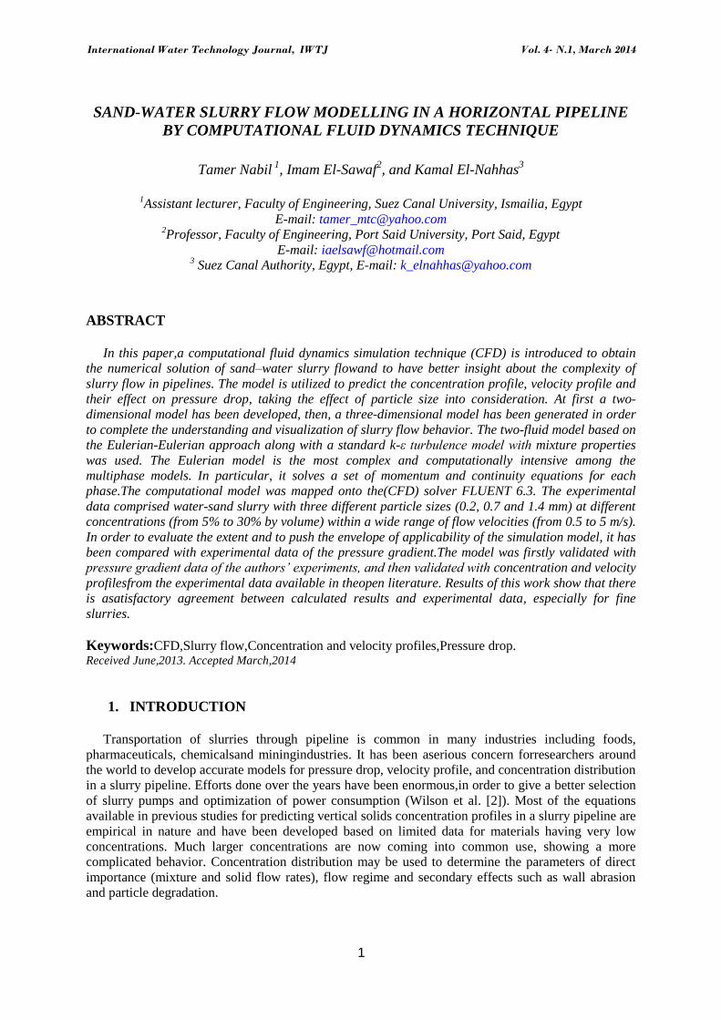
Fluid-solid momentum equation

The conservation of momentum for the Sth solid phase is:

∂

∂t αsρsvs + . αsρsvs vs

= −αsp − ps + . τs + αsρsg

+ αsρs Fs + Flift ,s

+ FVm ,s + Kls vl − vs + mls vls

N

l=1

(4)

where mpq , mls characterizethe mass transfer rate per unit volume between phases. From the mass

conservation mpq =−mqp , mls =−msl ,mpp =0 and mss =0.

Fluid-solid exchange coefficient

The fluid-solid exchange coefficient Ksl is in the following general form;

Ksl =αsρsf

τs (5)

τs =ρsds

2

18μl

(6)

wheref is defined differently for the different exchange-coefficient models. All definitions of f include

a drag function (CD) that is based on the relative Reynolds number (Res). It is the drag function that

differs among the exchange coefficient models. Three models are widely used for calculating solid-

liquid interaction:Wen and Yu model, Syamlal-O'Brien model and Gidaspow model.

Solid-solid exchange coefficient

The solid-solid exchange coefficient Kls has the following form:

Kls =3 1 + els

π

2+ Cfr ,ls

π2

8 αsρsαlρl dl + ds

2go,ls

2π ρldl3 + ρsds

3 vl − vs (7)

2.1.3 Solids Shear Stresses

The stress tensor of solids contains shear and bulk viscosities arising from particle momentum

exchange due to translation and collision(Liangyong et al. [10]). The collision and kinetic parts, and

the optional frictional part, are added to give the solids shear viscosity:

µs = µs,col + µs,kin − µs,fr (8)

µs,col =4

5αsρsds go,ss 1 + ess

θs

π

0.5

(9)

µs,kin =αsdsρs πθs

6 3 − ess 1 +

2

5 1 + ess 3ess − 1 αsgo,ss (10)

µs,fr =ps sinΦ

2 I2D

(11)

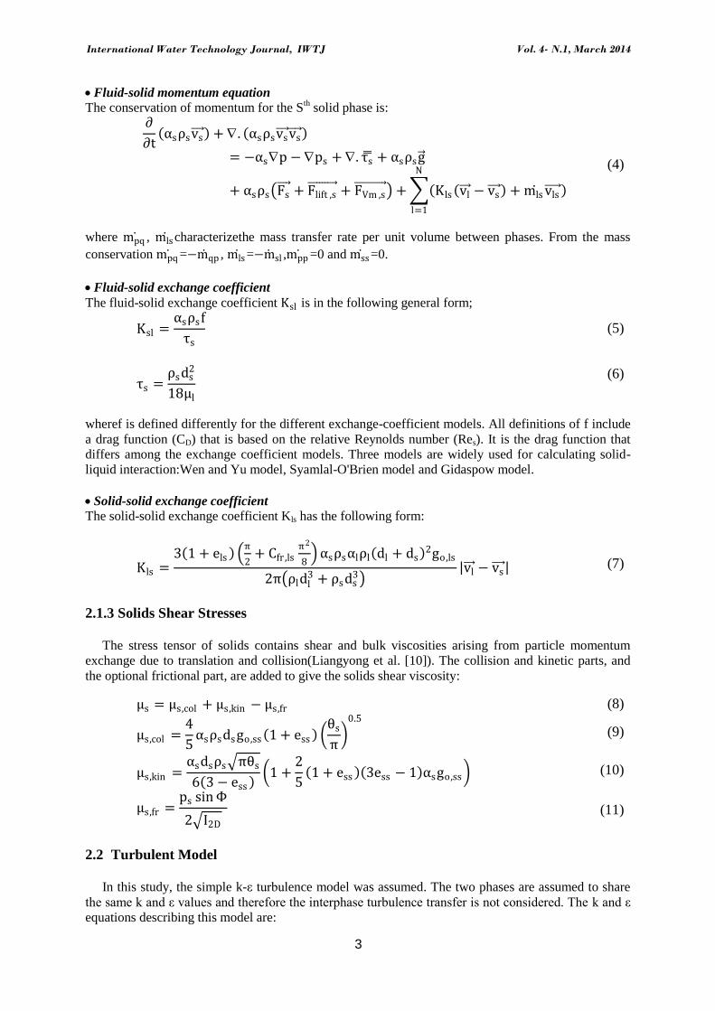
2.2 Turbulent Model

In this study, the simple k-ε turbulence model was assumed. The two phases are assumed to share

the same k and ε values and therefore the interphase turbulence transfer is not considered. The k and ε

equations describing this model are:


4

∂

∂t ρm k + . ρm vm k = .

µt,m

ςkk + Gk,m − ρmε (12)

∂

∂t ρmε + . ρm vm ε = .

µt,m

ςεε +

ε

k C1εGk,m − C2ερmε (13)

3. DESCRIPTION OF THE TWO DIMENSIONAL CFD SIMULATION

Initially, the simulation was setup in two dimensions. “Gambit” is one of the softwares in which

the geometry can be setup and meshes can be generated. Rectangular pipe geometry (same pipe

dimension as in the experiment) wascreated.The pipe length, L, was much higherthan the maximum

entrance length, Le, required for a fully developed flow (L/D<200). The geometry was meshed into

approximately 1.5×105 tetrahedral cells.For Eulerian slurry calculations, we use the Phase Coupled

SIMPLE (PC-SIMPLE) algorithm, for the pressure-velocity coupling.Simulations of the carrier fluid

flowing alone were performed first, to serve both as an initial validation of the code and the numerical

grid, and to reveal the effects of solid particles on the liquid velocity (by deselecting the volume

fraction equations). Once the initial solution for the primary phase was obtained, the volume fraction

equations were turned back on and the calculation continued with all the phases present.

The first-order upwind discretization scheme was used for the volume fraction, momentum

equations, turbulence kinetic energy (k), and turbulence dissipation rate (ε). All the simulations were

performed in double numerical precision. Mean velocity as an inletboundary condition and pressure as

an outlet boundary conditionwereimposed at the inlet and outlet of the slurry pipeline. The

homogeneous volumetric fraction of each phase was specified at the inlet. The usual no-slip boundary

condition was adopted at the pipe wall. To avoid divergence, under-relaxation technique was applied.

The solution was assumed to have converged when the mass and momentum residuals reached 10-4

for

all of the solved equations.

4. EXPERIMENTAL SETUP AND MEASURING FACILITIES

An open-loop recirculation pipeline system, shown schematically in Figure (1), was employed for

testing the slurry flow behavior (hydraulic resistance curves, Figures 14, 15 and 16). A stainless steel

pipe loop of internal diameter 26.8mm was used for slurry parameters measurement (pressure drop).

The test section is located in the back (downstream) branch of the piping loop system. A transparent

section was mounted at the end of the test section. Pressure measurements were obtained over two

sections of the pipe. The pressure is transmitted from the tapping points to three pressure

transducersthrough transmission lines and transparent Perspexsedimentation vessels filled with pure

water. The control and calibration unit is used to calibrate the sensitive pressure transducers, control

different passes to let the transducers read the pressure of any test point and to protect the

pump.Pressure transducers were used to measure the pressure losses between the pressure taps. The

output signalsof the transducers, which are proportional to the applied pressure, weredisplayed as an

analogue value (in milli-ampere). Also these analogue signals were converted into digital signals by

adata acquisition system.The digital data were entered in a computer, which is equippedwith the

LABVIEW software,enabling online measurement, analysis and storage of the data.

At the downstream end of the test pipes a box divider was mounted,allowing thedischarge to be

diverted to a plastic container. Since the divider arm was connected to an electric stopwatch, the mass

flow rate wasmeasured,the slurry density and hence the volumetric concentration could be determined.

Three sorts of the mono-disperse quartz sands, ρs=2650kg/m3, were used for preparing slurries of the

experiments; fine (d50=0.2mm), medium (d50=0.7mm) and coarse (d50=1.4mm). The volumetric

concentrations of solids ranged from Cv=5% to 30%.

Due to unavailable feasibility the experimental data of the concentration distributions and velocity

profile werecollected from literature, Matousek et al. [5] and Gillies [4], for sand water flow system.


5

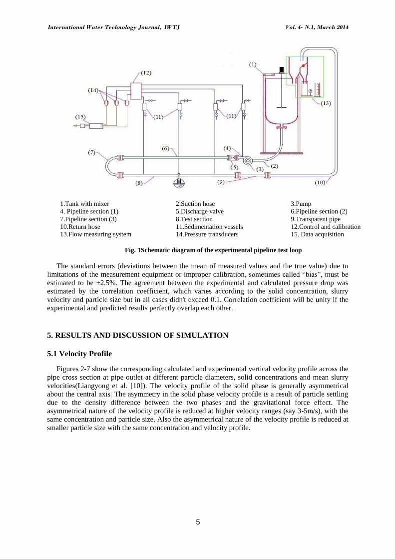
1.Tank with mixer 2.Suction hose 3.Pump

4. Pipeline section (1) 5.Discharge valve 6.Pipeline section (2)

7.Pipeline section (3) 8.Test section 9.Transparent pipe

10.Return hose 11.Sedimentation vessels 12.Control and calibration

13.Flow measuring system 14.Pressure transducers 15. Data acquisition

Fig. 1Schematic diagram of the experimental pipeline test loop

The standard errors (deviations between the mean of measured values and the true value) due to

limitations of the measurement equipment or improper calibration, sometimes called “bias”, must be

estimated to be ±2.5%. The agreement between the experimental and calculated pressure drop was

estimated by the correlation coefficient, which varies according to the solid concentration, slurry

velocity and particle size but in all cases didn't exceed 0.1. Correlation coefficient will be unity if the

experimental and predicted results perfectly overlap each other.

5. RESULTS AND DISCUSSION OF SIMULATION

5.1 Velocity Profile

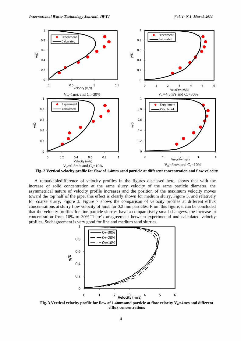
Figures 2-7 show the corresponding calculated and experimental vertical velocity profile across the

pipe cross section at pipe outlet at different particle diameters, solid concentrations and mean slurry

velocities(Liangyong et al. [10]). The velocity profile of the solid phase is generally asymmetrical

about the central axis. The asymmetry in the solid phase velocity profile is a result of particle settling

due to the density difference between the two phases and the gravitational force effect. The

asymmetrical nature of the velocity profile is reduced at higher velocity ranges (say 3-5m/s), with the

same concentration and particle size. Also the asymmetrical nature of the velocity profile is reduced at

smaller particle size with the same concentration and velocity profile.


6

Fig. 2 Vertical velocity profile for flow of 1.4mm sand particle at different concentration and flow velocity

A remarkabledifference of velocity profiles in the figures discussed here, shows that with the

increase of solid concentration at the same slurry velocity of the same particle diameter, the

asymmetrical nature of velocity profile increases and the position of the maximum velocity moves

toward the top half of the pipe; this effect is clearly shown for medium slurry, Figure 5, and relatively

for coarse slurry, Figure 3. Figure 7 shows the comparison of velocity profiles at different efflux

concentrations at slurry flow velocity of 5m/s for 0.2 mm particles. From this figure, it can be concluded

that the velocity profiles for fine particle slurries have a comparatively small changevs. the increase in

concentration from 10% to 30%.There‟s anagreement between experimental and calculated velocity

profiles. Suchagreement is very good for fine and medium sand slurries.

Fig. 3 Vertical velocity profile for flow of 1.4mmsand particle at flow velocity Vm=4m/s and different

efflux concentrations

0

0.2

0.4

0.6

0.8

1

0 0.5 1 1.5

y/D

Velocity (m/s)

Experiment

Calculated

0

0.2

0.4

0.6

0.8

1

0 1 2 3 4 5 6

y/D

Velocity (m/s)

Experiment

Calculated

0

0.2

0.4

0.6

0.8

1

0 0.2 0.4 0.6 0.8 1

y/D

Velocity (m/s)

Experiment

Calculated

0

0.2

0.4

0.6

0.8

1

0 1 2 3 4

y/D

Velocity (m/s)

Experiment

Calculated

0

0.2

0.4

0.6

0.8

1

0 1 2 3 4 5 6

y/D

Velocity (m/s)

Cv=30%

Cv=20%

Cv=10%

Vm=4.5m/s and Cv=30% Vm=1m/s and Cv=30%

Vm=3m/s and Cv=10% Vm=0.5m/s and Cv=10%


7

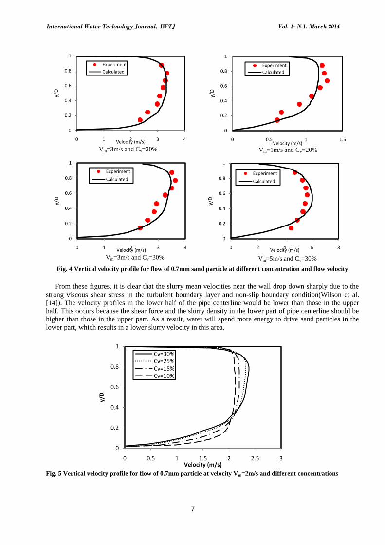
Fig. 4 Vertical velocity profile for flow of 0.7mm sand particle at different concentration and flow velocity

From these figures, it is clear that the slurry mean velocities near the wall drop down sharply due to the

strong viscous shear stress in the turbulent boundary layer and non-slip boundary condition(Wilson et al.

[14]). The velocity profiles in the lower half of the pipe centerline would be lower than those in the upper

half. This occurs because the shear force and the slurry density in the lower part of pipe centerline should be

higher than those in the upper part. As a result, water will spend more energy to drive sand particles in the

lower part, which results in a lower slurry velocity in this area.

Fig. 5 Vertical velocity profile for flow of 0.7mm particle at velocity Vm=2m/s and different concentrations

0

0.2

0.4

0.6

0.8

1

0 1 2 3 4

y/D

Velocity (m/s)

Experiment

Calculated

0

0.2

0.4

0.6

0.8

1

0 0.5 1 1.5

y/D

Velocity (m/s)

Experiment

Calculated

0

0.2

0.4

0.6

0.8

1

0 1 2 3 4

y/D

Velocity (m/s)

Experiment

Calculated

0

0.2

0.4

0.6

0.8

1

0 2 4 6 8

y/D

Velocity (m/s)

Experiment

Calculated

0

0.2

0.4

0.6

0.8

1

0 0.5 1 1.5 2 2.5 3

y/D

Velocity (m/s)

Cv=30%Cv=25%Cv=15%Cv=10%

Vm=1m/s and Cv=20% Vm=3m/s and Cv=20%



8

Fig. 6 Vertical velocity profile for flow of 0.2mm sand particle at differentconcentration and flow velocity

Fig. 7 Vertical velocity profile for flow of 0.2mm particle at velocity Vm=5m/s and different concentrations

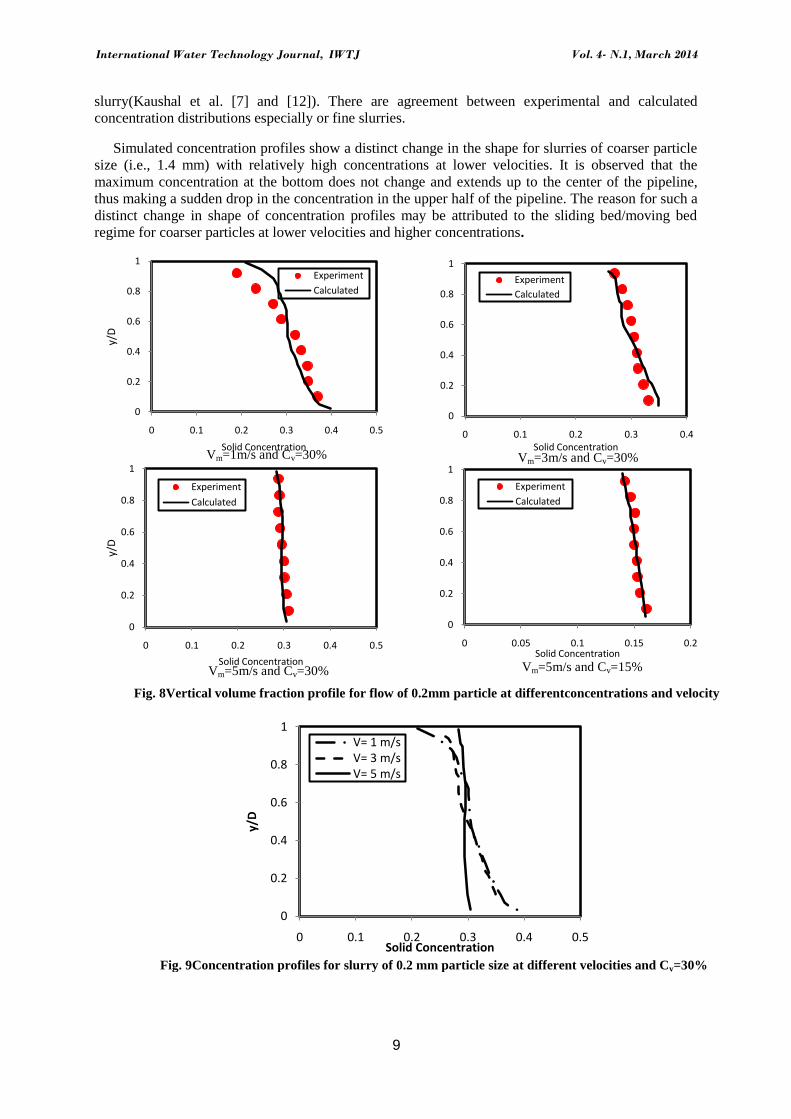
5.2 Concentration Profile

Figures 8-13 show the calculated and experimental vertical concentration profiles across the pipe

cross section at the pipe outlet. These figures show profiles of concentrations of solid at the pipe outlet

at different particle diameter, flow velocities and efflux concentration. Data representation used in

these pictures helpsunderstanding the distribution of solids across a cross sectionof the pipe. This is

one of the biggest advantages of CFD, which helps to generate such type of concentration contour.

Figures 8-13show the predicted volume concentration profiles along the vertical diameter at

various influx velocities, sand particle diameter and sand volume fraction. It is observed that the

particles are asymmetrically distributed in the vertical plane with the degree of asymmetry increasing

with increase in particle size because of the gravitational effect. It is also observed that the degree of

asymmetry for the same overall concentration of slurry increases with decreasing flow

velocity(Seshadri et al. [15]). This is expected, because with a decrease in flow velocity there will be a

decrease in turbulent energy, which is responsible for keeping the solids in suspension.

From these figures, it is also observed that for a given velocity, increasing concentration reduces

the asymmetry because of enhanced interference effect between solid particles. The effect of this

interference is so strong that the asymmetry even at lower velocities is very much reduced at higher

concentrations. Therefore, it can be concluded that the degree of asymmetry in the concentration

profiles in the vertical plane depends upon particle size, flow velocity and overall concentration of

0

0.2

0.4

0.6

0.8

1

0 0.5 1 1.5 2 2.5

y/D

Velocity (m/s)

Experiment

Calculated

0

0.2

0.4

0.6

0.8

1

0 1 2 3 4

y/D

Velocity (m/s)

Experiment

Calculated

0

0.2

0.4

0.6

0.8

1

0 2 4 6 8

y/D

Velocity (m/s)

Cv=30%

Cv=20%

Cv=10%



9

slurry(Kaushal et al. [7] and [12]). There are agreement between experimental and calculated

concentration distributions especially or fine slurries.

Simulated concentration profiles show a distinct change in the shape for slurries of coarser particle

size (i.e., 1.4 mm) with relatively high concentrations at lower velocities. It is observed that the

maximum concentration at the bottom does not change and extends up to the center of the pipeline,

thus making a sudden drop in the concentration in the upper half of the pipeline. The reason for such a

distinct change in shape of concentration profiles may be attributed to the sliding bed/moving bed

regime for coarser particles at lower velocities and higher concentrations.

Fig. 8Vertical volume fraction profile for flow of 0.2mm particle at differentconcentrations and velocity

Fig. 9Concentration profiles for slurry of 0.2 mm particle size at different velocities and Cv=30%

0

0.2

0.4

0.6

0.8

1

0 0.1 0.2 0.3 0.4 0.5

y/D

Solid Concentration

Experiment

Calculated

0

0.2

0.4

0.6

0.8

1

0 0.1 0.2 0.3 0.4Solid Concentration

Experiment

Calculated

0

0.2

0.4

0.6

0.8

1

0 0.1 0.2 0.3 0.4 0.5

y/D

Solid Concentration

Experiment

Calculated

0

0.2

0.4

0.6

0.8

1

0 0.05 0.1 0.15 0.2Solid Concentration

Experiment

Calculated

0

0.2

0.4

0.6

0.8

1

0 0.1 0.2 0.3 0.4 0.5

y/D

Solid Concentration

V= 1 m/sV= 3 m/sV= 5 m/s




10

Fig. 10Vertical volume fraction profile for flow of 0.7mm particle at differentconcentrations and velocity

Fig. 11 Concentration profiles for slurry of 0.7 mm particle size at different velocities and Cv=30%

0

0.2

0.4

0.6

0.8

1

0 0.1 0.2 0.3 0.4 0.5

y/D

Solid Concentration

Experiment

Calculated

0

0.2

0.4

0.6

0.8

1

0 0.1 0.2 0.3 0.4 0.5

y/D

Solid Concentration

Experiment

Calculated

0

0.2

0.4

0.6

0.8

1

0 0.1 0.2 0.3 0.4 0.5

y/D

Solid Concentration

Experiment

Calculated

0

0.2

0.4

0.6

0.8

1

0 0.1 0.2 0.3 0.4

y/D

Solid concentration

Experiment

Calculated

0

0.2

0.4

0.6

0.8

1

0 0.05 0.1 0.15 0.2 0.25

y/D

Solid Concentration

Experiment

Calculated

0

0.2

0.4

0.6

0.8

1

0 0.05 0.1 0.15 0.2

y/D

Solid Concentration

Experiment

Calculated

0

0.2

0.4

0.6

0.8

1

0 0.1 0.2 0.3 0.4 0.5

y/D

Solid Concentration

V = 5 m/s

V = 3 m/s

V = 1 m/s

Vm=3m/s and Cv=30%

Vm=5m/s

and

Cv=30%

Vm=3m/s

and

Cv=30%

Vm=5m/s and Cv=30%

Vm=1m/s and Cv=12%

Vm=5m/s

and

Cv=30%

Vm=3m/s

and

Cv=30%

Vm=1m/s and Cv=30%

Vm=5m/s

and

Cv=30%

Vm=3m/s

and

Cv=30%

Vm=5m/s and Cv=12%

Vm=5m/s

and

Cv=30%

Vm=3m/s

and

Cv=30%

Vm=3m/s and Cv=12%

Vm=5m/s

and

Cv=30%

Vm=3m/s

and

Cv=30%


11

Fig. 12 Vertical volume fraction profile for flow of 1.4mm particle at differentconcentrations and velocity

Fig. 13 Concentration profiles for slurry of 1.4 mm particle size at different velocities and Cv=15%

0

0.2

0.4

0.6

0.8

1

0 0.1 0.2 0.3 0.4 0.5

y/D

Solid Concentration

Experiment

Calculated

0

0.2

0.4

0.6

0.8

1

0 0.1 0.2 0.3 0.4

y/D

Solid Concentration

Experiment

Calculated

0

0.2

0.4

0.6

0.8

1

0 0.1 0.2 0.3 0.4

y/D

Solid Concentration

Experiment

Calculated

0

0.2

0.4

0.6

0.8

1

0 0.2 0.4 0.6 0.8

y/D

Solid Concentration

Experiment

Calculated

0

0.2

0.4

0.6

0.8

1

0 0.2 0.4 0.6

y/D

Solid Concentration

Experiment

Calculated

0

0.2

0.4

0.6

0.8

1

0 0.05 0.1 0.15 0.2

y/D

Solid Concentration

Experiment

Calculated

0

0.2

0.4

0.6

0.8

1

0 0.1 0.2 0.3 0.4 0.5

y/D

Solid Concentration

V = 1 m/s

V = 0.5 m/s

V = 3 m/s


Vm=1m/s and Cv=15% Vm=0.5m/s and Cv=15%



12

Due to the difference in solid concentration across the pipe diameter the drag coefficient and the

settling velocity arenot constant throughout the pipe cross section and they vary along with the

concentration. This non uniform distribution of drag coefficient and settling velocity give rise to

different solid liquid exchange coefficients across pipe cross section. The simulation model could not

capture these variations so there are some variations of the experimental results and the calculated

concentration profiles that appear to be non-smooth.

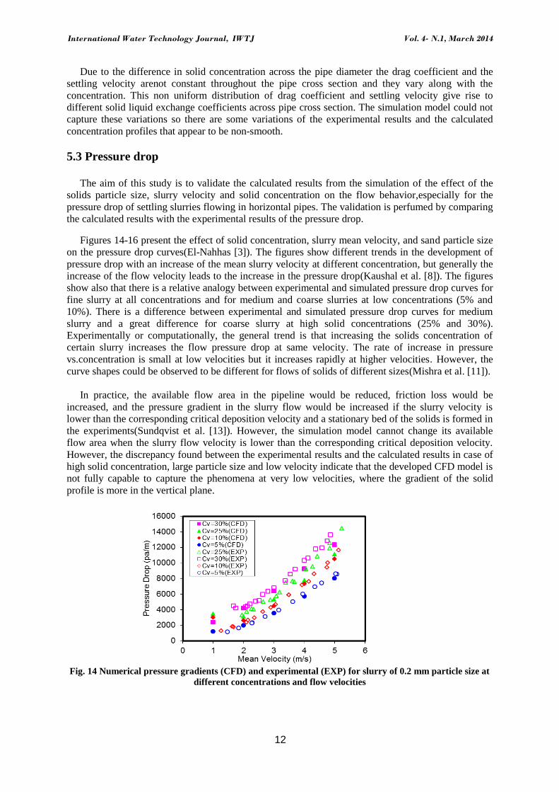
5.3 Pressure drop

The aim of this study is to validate the calculated results from the simulation of the effect of the

solids particle size, slurry velocity and solid concentration on the flow behavior,especially for the

pressure drop of settling slurries flowing in horizontal pipes. The validation is perfumed by comparing

the calculated results with the experimental results of the pressure drop.

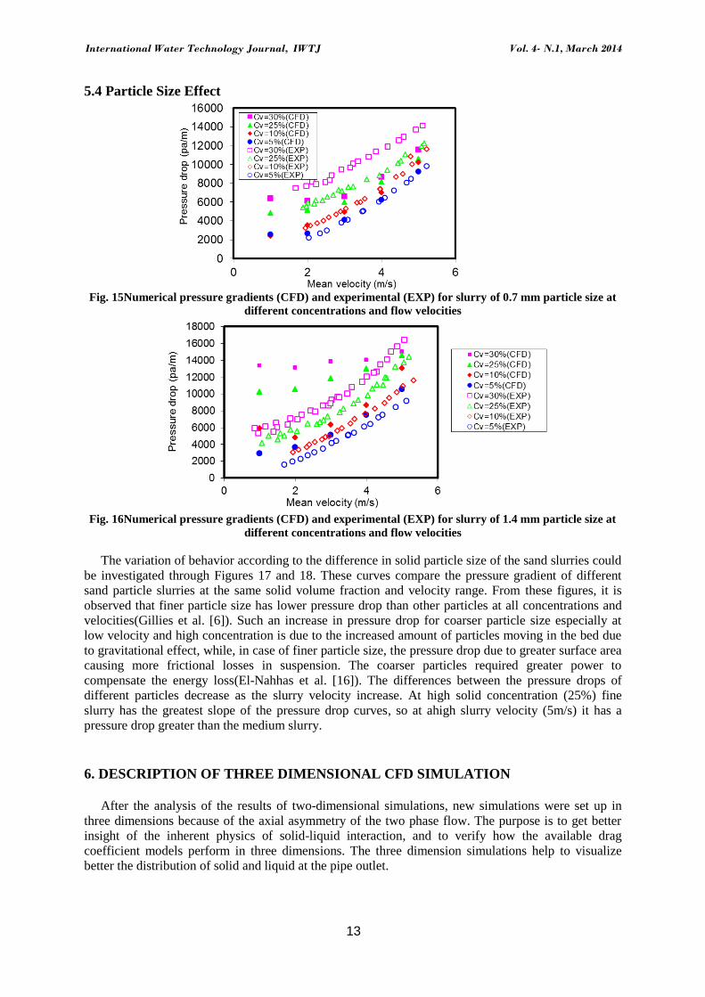
Figures 14-16 present the effect of solid concentration, slurry mean velocity, and sand particle size

on the pressure drop curves(El-Nahhas [3]). The figures show different trends in the development of

pressure drop with an increase of the mean slurry velocity at different concentration, but generally the

increase of the flow velocity leads to the increase in the pressure drop(Kaushal et al. [8]). The figures

show also that there is a relative analogy between experimental and simulated pressure drop curves for

fine slurry at all concentrations and for medium and coarse slurries at low concentrations (5% and

10%). There is a difference between experimental and simulated pressure drop curves for medium

slurry and a great difference for coarse slurry at high solid concentrations (25% and 30%).

Experimentally or computationally, the general trend is that increasing the solids concentration of

certain slurry increases the flow pressure drop at same velocity. The rate of increase in pressure

vs.concentration is small at low velocities but it increases rapidly at higher velocities. However, the

curve shapes could be observed to be different for flows of solids of different sizes(Mishra et al. [11]). In practice, the available flow area in the pipeline would be reduced, friction loss would be

increased, and the pressure gradient in the slurry flow would be increased if the slurry velocity is

lower than the corresponding critical deposition velocity and a stationary bed of the solids is formed in

the experiments(Sundqvist et al. [13]). However, the simulation model cannot change its available

flow area when the slurry flow velocity is lower than the corresponding critical deposition velocity.

However, the discrepancy found between the experimental results and the calculated results in case of

high solid concentration, large particle size and low velocity indicate that the developed CFD model is

not fully capable to capture the phenomena at very low velocities, where the gradient of the solid

profile is more in the vertical plane.

Fig. 14 Numerical pressure gradients (CFD) and experimental (EXP) for slurry of 0.2 mm particle size at

different concentrations and flow velocities


13

5.4 Particle Size Effect

Fig. 15Numerical pressure gradients (CFD) and experimental (EXP) for slurry of 0.7 mm particle size at


Fig. 16Numerical pressure gradients (CFD) and experimental (EXP) for slurry of 1.4 mm particle size at


The variation of behavior according to the difference in solid particle size of the sand slurries could

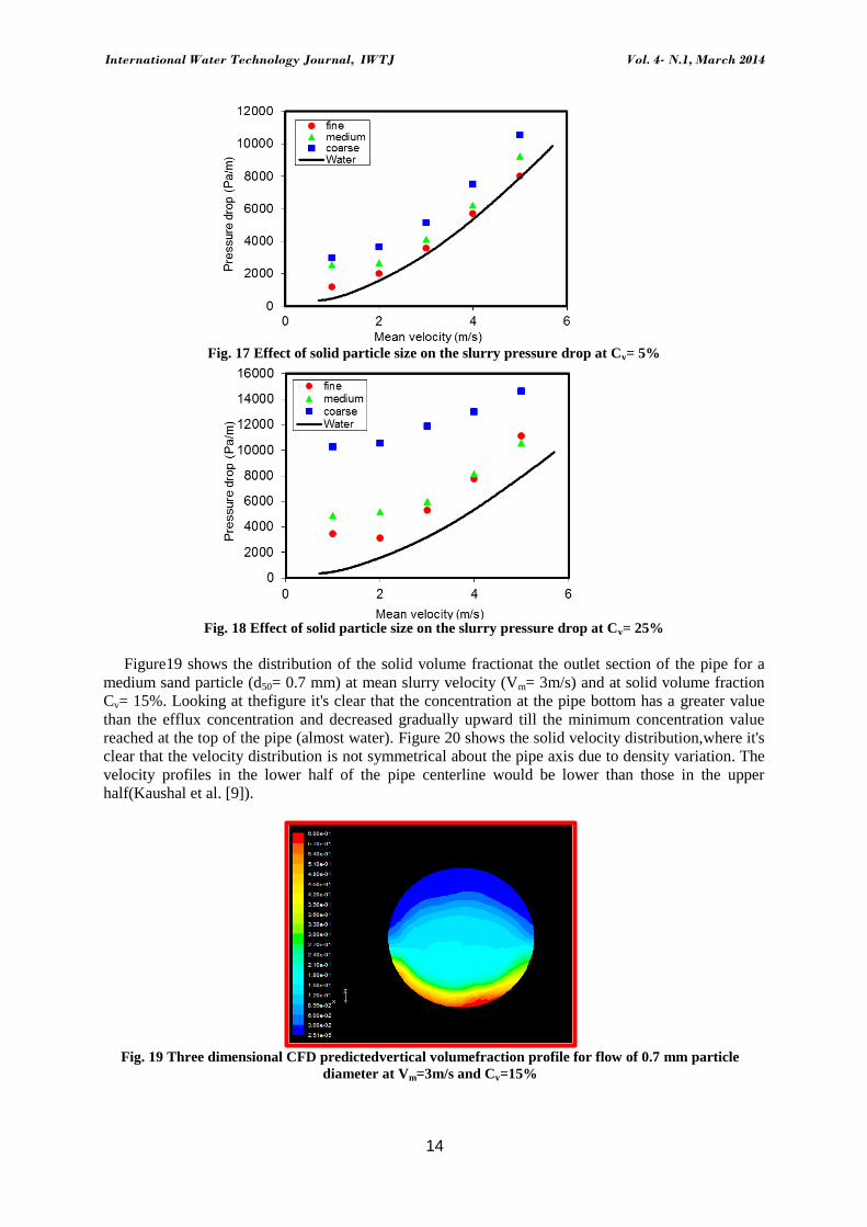
be investigated through Figures 17 and 18. These curves compare the pressure gradient of different

sand particle slurries at the same solid volume fraction and velocity range. From these figures, it is

observed that finer particle size has lower pressure drop than other particles at all concentrations and

velocities(Gillies et al. [6]). Such an increase in pressure drop for coarser particle size especially at

low velocity and high concentration is due to the increased amount of particles moving in the bed due

to gravitational effect, while, in case of finer particle size, the pressure drop due to greater surface area

causing more frictional losses in suspension. The coarser particles required greater power to

compensate the energy loss(El-Nahhas et al. [16]). The differences between the pressure drops of

different particles decrease as the slurry velocity increase. At high solid concentration (25%) fine

slurry has the greatest slope of the pressure drop curves, so at ahigh slurry velocity (5m/s) it has a

pressure drop greater than the medium slurry.

6. DESCRIPTION OF THREE DIMENSIONAL CFD SIMULATION

After the analysis of the results of two-dimensional simulations, new simulations were set up in

three dimensions because of the axial asymmetry of the two phase flow. The purpose is to get better

insight of the inherent physics of solid-liquid interaction, and to verify how the available drag

coefficient models perform in three dimensions. The three dimension simulations help to visualize

better the distribution of solid and liquid at the pipe outlet.


14

Fig. 17 Effect of solid particle size on the slurry pressure drop at Cv= 5%

Fig. 18 Effect of solid particle size on the slurry pressure drop at Cv= 25%

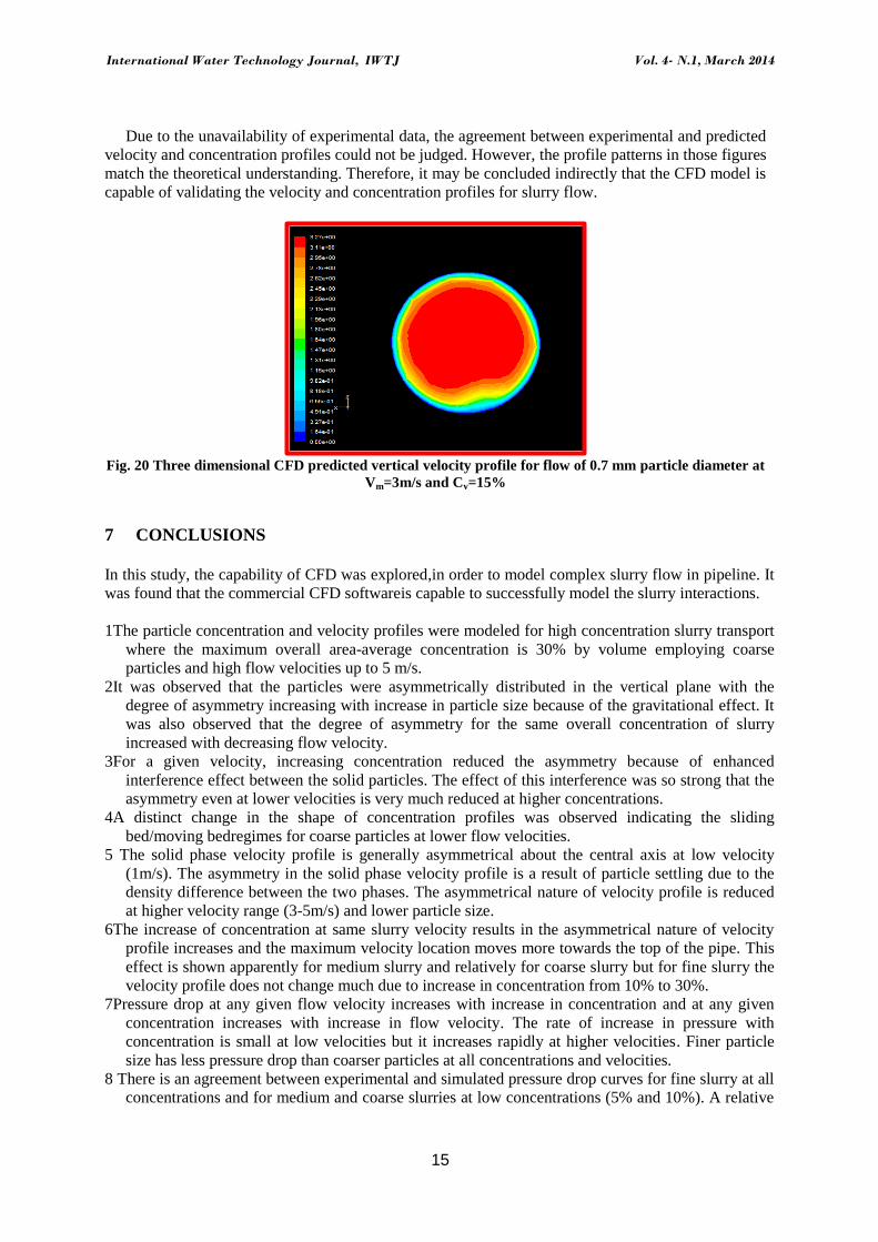
Figure19 shows the distribution of the solid volume fractionat the outlet section of the pipe for a

medium sand particle (d50= 0.7 mm) at mean slurry velocity (Vm= 3m/s) and at solid volume fraction

Cv= 15%. Looking at thefigure it's clear that the concentration at the pipe bottom has a greater value

than the efflux concentration and decreased gradually upward till the minimum concentration value

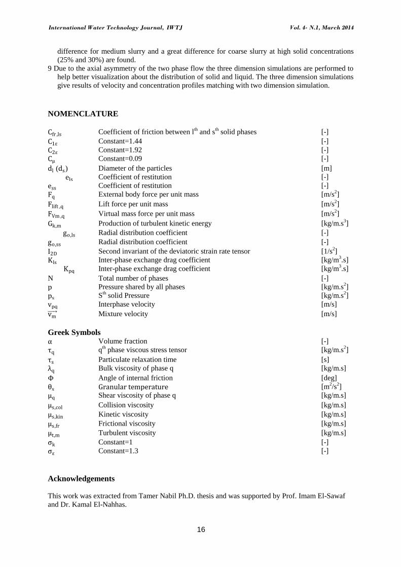
reached at the top of the pipe (almost water). Figure 20 shows the solid velocity distribution,where it's

clear that the velocity distribution is not symmetrical about the pipe axis due to density variation. The

velocity profiles in the lower half of the pipe centerline would be lower than those in the upper

half(Kaushal et al. [9]).

Fig. 19 Three dimensional CFD predictedvertical volumefraction profile for flow of 0.7 mm particle

diameter at Vm=3m/s and Cv=15%


15

Due to the unavailability of experimental data, the agreement between experimental and predicted

velocity and concentration profiles could not be judged. However, the profile patterns in those figures

match the theoretical understanding. Therefore, it may be concluded indirectly that the CFD model is

capable of validating the velocity and concentration profiles for slurry flow.

Fig. 20 Three dimensional CFD predicted vertical velocity profile for flow of 0.7 mm particle diameter at

Vm=3m/s and Cv=15%

7 CONCLUSIONS

In this study, the capability of CFD was explored,in order to model complex slurry flow in pipeline. It

was found that the commercial CFD softwareis capable to successfully model the slurry interactions.

1The particle concentration and velocity profiles were modeled for high concentration slurry transport

where the maximum overall area-average concentration is 30% by volume employing coarse

particles and high flow velocities up to 5 m/s.

2It was observed that the particles were asymmetrically distributed in the vertical plane with the

degree of asymmetry increasing with increase in particle size because of the gravitational effect. It

was also observed that the degree of asymmetry for the same overall concentration of slurry

increased with decreasing flow velocity.

3For a given velocity, increasing concentration reduced the asymmetry because of enhanced

interference effect between the solid particles. The effect of this interference was so strong that the

asymmetry even at lower velocities is very much reduced at higher concentrations.

4A distinct change in the shape of concentration profiles was observed indicating the sliding

bed/moving bedregimes for coarse particles at lower flow velocities.

5 The solid phase velocity profile is generally asymmetrical about the central axis at low velocity

(1m/s). The asymmetry in the solid phase velocity profile is a result of particle settling due to the

density difference between the two phases. The asymmetrical nature of velocity profile is reduced

at higher velocity range (3-5m/s) and lower particle size.

6The increase of concentration at same slurry velocity results in the asymmetrical nature of velocity

profile increases and the maximum velocity location moves more towards the top of the pipe. This

effect is shown apparently for medium slurry and relatively for coarse slurry but for fine slurry the

velocity profile does not change much due to increase in concentration from 10% to 30%.

7Pressure drop at any given flow velocity increases with increase in concentration and at any given

concentration increases with increase in flow velocity. The rate of increase in pressure with

concentration is small at low velocities but it increases rapidly at higher velocities. Finer particle

size has less pressure drop than coarser particles at all concentrations and velocities.

8 There is an agreement between experimental and simulated pressure drop curves for fine slurry at all

concentrations and for medium and coarse slurries at low concentrations (5% and 10%). A relative


16

difference for medium slurry and a great difference for coarse slurry at high solid concentrations

(25% and 30%) are found. 9 Due to the axial asymmetry of the two phase flow the three dimension simulations are performed to

help better visualization about the distribution of solid and liquid. The three dimension simulations

give results of velocity and concentration profiles matching with two dimension simulation.

NOMENCLATURE

Cfr ,ls Coefficient of friction between l

th and s

th solid phases [-]

C1ε Constant=1.44 [-]

C2ε Constant=1.92 [-]

Cµ Constant=0.09 [-]

dl (ds) Diameter of the particles [m]

els Coefficient of restitution [-]

ess Coefficient of restitution [-]

Fq External body force per unit mass [m/s2]

Flift ,q Lift force per unit mass [m/s2]

FVm ,q Virtual mass force per unit mass [m/s2]

Gk,m Production of turbulent kinetic energy [kg/m.s3]

go,ls Radial distribution coefficient [-]

go,ss Radial distribution coefficient [-]

I2D Second invariant of the deviatoric strain rate tensor [1/s2]

Kls Inter-phase exchange drag coefficient [kg/m3.s]

Kpq Inter-phase exchange drag coefficient [kg/m3.s]

N Total number of phases [-]

p Pressure shared by all phases [kg/m.s2]

ps Sth solid Pressure [kg/m.s

2]

vpq Interphase velocity [m/s]

vm Mixture velocity [m/s]

Greek Symbols

α Volume fraction [-]

τq qth phase viscous stress tensor [kg/m.s

2]

τs Particulate relaxation time [s]

λq Bulk viscosity of phase q [kg/m.s]

Φ Angle of internal friction [deg]

θs Granular temperature [m2/s

2]

µq Shear viscosity of phase q [kg/m.s]

µs,col Collision viscosity [kg/m.s]

µs,kin Kinetic viscosity [kg/m.s]

µs,fr Frictional viscosity [kg/m.s]

µt,m Turbulent viscosity [kg/m.s]

ςk Constant=1 [-]

ςε Constant=1.3 [-]

Acknowledgements

This work was extracted from Tamer Nabil Ph.D. thesis and was supported by Prof. Imam El-Sawaf

and Dr. Kamal El-Nahhas.


17

REFERENCES

[1] Anderson, J.D.,Computational Fluid Dynamics, The Basic and Applications, McGraw-Hill, New

york, pp.37-82, 1995.

[2] Wilson, K. C., Addie, G. R. and Clift, R.,Slurry Transport Using Centrifugal Pumps, London,

1992.

[3] El-Nahhas, K.,Hydraulic Transport of Dense Fine-Grained Suspensions, Ph.D. Thesis, Faculty of

Engineering at Port Said, Port Said University, Egypt, 2002.

[4] Gillies, R.G., Pipeline Flow of Coarse Particle Slurries, Ph.D. thesis, University of Saskatchewan,

Saskatoon, 1993.

[5] Matousek, V., Flow Mechanism of Sand-Water Mixtures in Pipelines, Ph.D. thesis, Delft

University, Netherlands, 1997.

[6] Gillies, R.G. and Shook, C.A., Modelling High Concentration Settling Slurry Flows, The Canadian

Journal of Chemical Eng. 78, pp.709–716, 2000.

[7] Kaushal, D.R. and Tomita, Y., Solid Concentration Profiles and Pressure Drop in Pipeline Flow of

MultisizedParticulate Slurries,Int. journal of multiphase flow 28, pp.1697-1717, 2002.

[8] Kaushal, D.R. and Tomita, Y., Comparative Study of Pressure Drop in Multisized Particulate

Slurry Flow Through Pipe and Rectangular Duct, Int. J. of Multiphase Flow, vol. 29, 1473–1487,

2003.

[9] Kaushal, D.R., Thinglas, T., Tomita, Y., Kuchii, S. and Tsukamoto, H., CFD modeling for pipeline

flow of fine particles at high concentration, Int. J. of Multiphase Flow 43, pp.85–100, 2012.

[10] Liangyong Chen, YufengDuan, WenhaoPu, and Changsui Zhao, CFD Simulation of Coal-Water

Slurry Flowing in Horizontal Pipelines, Korean J. Chem. Eng., 26(4), pp. 1144-1154, 2009.

[11] Mishra, R. and Seshadri, V., Improved Model for Prediction of Pressure Drop and Velocity Field

in Multisized Particulate Slurry Flow Through Horizontal Pipes, Powder Handling and

Processing Journal 10, pp. 279–289, 1998.

[12] Kaushal, D.R. and Tomita, Y., Concentration at the Pipe Bottom at Deposition Velocity for

Transportation of Commercial Slurries Through Pipeline, Powder Technology 125, pp. 89–101,

2002.

[13] Sundqvist, A., Sellgren, A. and Addie, G., Slurry Pipeline Friction Losses for Coarse and High

Density Products,Powder Tech. 89, pp. 19–28, 1996.

[14] Wilson, K.C., Sanders, R.S., Gillies R.G. and Shook C.A, Verification of the Near-Wall Model

for Slurry Flow, Powder Tech. 197, pp. 247–253, 2010.

[15] Seshadri, V. and Malhotra, R.C., Concentration and Size Distribution of Solids in Slurry Pipeline,

Proc. 11th National Conf. on Fluid Mechanics and Fluid Power, India, pp.110–123, 1982.

[16] El-Nahhas, K., Abu-Rayan, M. and El-Sawaf, I. A., Flow Behaviour of Coarse-Grained Settling

Slurries, Proc. 12th International Water Tech. Conference, Alexandria, Egypt, 2008.

Documents

SAND-WATER SLURRY FLOW MODELLING IN A ...iwtj.info/wp-content/uploads/2014/06/V.4-N.1-P.13.pdfSAND-WATER SLURRY FLOW MODELLING IN A HORIZONTAL PIPELINE BY COMPUTATIONAL FLUID DYNAMICS