University of California,Santa Barbara

Senior Thesis

Sard’s Theorem andApplications

Author:Lingyu Du

Supervisor:Dr. Andrew

Cotton-Clay

May 31, 2016

Acknowledgements

I would like to express my sincerest gratitude to my supervisor Prof. AndrewCotton-Clay, without whose valuable knowledge, explanations and time Icould not have written this thesis.

Abstract

This senior thesis consists of six chapters discussing the smooth maps of man-ifolds, and the aim is to provide an introduction to the structure of smoothmaps at their critical points. We will study immersions and submersions,and also present a proof of Sard’s theorem and some applications to topol-ogy based on Sard’s theorem.

Contents

1 Introduction 2

2 Background 42.1 Smooth Maps . . . . . . . . . . . . . . . . . . . . . . . . . . . 42.2 Manifolds . . . . . . . . . . . . . . . . . . . . . . . . . . . . . 62.3 Regular Value . . . . . . . . . . . . . . . . . . . . . . . . . . . 72.4 Measure Zero . . . . . . . . . . . . . . . . . . . . . . . . . . . 82.5 Theorems . . . . . . . . . . . . . . . . . . . . . . . . . . . . . 9

3 Immersions and Submersions 113.1 Immersions . . . . . . . . . . . . . . . . . . . . . . . . . . . . 113.2 Submersions . . . . . . . . . . . . . . . . . . . . . . . . . . . . 12

4 Sard’s Theorem 144.1 Easier cases . . . . . . . . . . . . . . . . . . . . . . . . . . . . 144.2 Proof of Sard’s theorem . . . . . . . . . . . . . . . . . . . . . 174.3 Examples . . . . . . . . . . . . . . . . . . . . . . . . . . . . . 20

5 Applications of Sard’s Theorem 215.1 Whitney Embedding Theorem . . . . . . . . . . . . . . . . . . 215.2 Morse Functions . . . . . . . . . . . . . . . . . . . . . . . . . . 225.3 Brouwer’s Fixed Point Theorem . . . . . . . . . . . . . . . . . 23

6 S2 is simply connected 266.1 Definitions . . . . . . . . . . . . . . . . . . . . . . . . . . . . . 266.2 Proof of S2 is simply connected . . . . . . . . . . . . . . . . . 27

7 Future Work 29

1

Chapter 1

Introduction

The aim of this thesis is to provide an introduction to Regular Value Theo-rem and Sard’s Theorem on manifolds and some applications.

Sard’s Theorem Let f : X → Y be a smooth map of manifolds, andlet C be the set of critical points of f in X. Then f(C) has measure zero in Y .

A critical point of a smooth map is a point of the domain at which thederivative does not have full rank. Our goal, then, is to discuss critical pointsof smooth maps and some applications on topology.

First of all, we will define the terms and prove some of their basic proper-ties, in order to provide the necessary background to help reader understandthe content we will talk about later. By smooth, we mean differentiable toall orders. By manifold, we mean a subset of Euclidean space. We will alsoillustrate examples and discuss diffeomorphisms.

The third chapter discusses immersions and submersions. We consider thelocal behavior of a smooth mapping, which leads to the immersion lemmaand submersion lemma, also leads us to regular value theorem, a key ingre-dient in our application of Sard’s Theorem. By regular value, we mean thaty ∈ V is called a regular value if dfx : Tx(U)→ Ty(V ) is onto at x such thatf(x) = y.

Regular Value Theorem If y ∈ Y is a regular value of f : X → Y thenf−1(y) is a manifold of dimension n−m, since dim(X) = n and dim(Y ) = m.

2

Next, we will present the theorem of Sard: the set of critical values ofa smooth map has measure zero. We will show that the inverse image of aregular value is a submanifold, and give both proofs of specific low dimensionversions of Sard’s Theorem and a general proof for Sard’s theorem in threesteps.

Finally, we will use Regular Value Theorem and Sard’s Theorem to presentsome important applications of manifolds, including the Whitney embeddingtheorem, the existence of Morse functions, and the Brouwer fixed point the-orem. For example, the Whitney Embedding Theorem that any smoothmanifold Mn ⊂ Rm has an injective immersion into R2n+1.

We will also use Sard’s Theorem to show that S2 is simply connectedbecause any smooth map of a circle must miss a point. We develop this withmention of polynomial approximation to deal with non-smooth loops, givinga full proof in the topological case.

3

Chapter 2

Background

This chapter provides the necessary background by giving the basic defini-tions, some examples and also some theorems that we will use in the futurechapters. First, let us explain some terms that we will use.

2.1 Smooth Maps

Rn denotes the n-dimensional euclidean space, and for x ∈ Rn, we obtainx = (x1, x2, · · · , xn), such that x1, x2 · · · , xn ∈ R which is the real numbers.Then we will define what is a smooth map.

Definition 2.1.1. Let U ⊂ Rn and V ⊂ Rk be open sets. A mapping f fromU to V written as f : U → V is a smooth map if all of the partial derivativesexist and are continuous.

More generally, we have the following.

Definition 2.1.2. Let X ⊂ Rn and Y ⊂ Rk be arbitrary subsets, and a mapf : X → Y is called smooth map if for every x ∈ X there exist an open setO ⊂ Rn that x ∈ O and a smooth mapping F : O → Rk that coincides withf throughout O ∩X.

Definition 2.1.3. Let U ⊂ Rn and V ⊂ Rk be open sets. For any smoothmap f : U → V , the derivative dfx : Rn → Rk is defined by the formuladfx(h) = lim

t→0(f(x+ th)−f(x))/t for x ∈ U , h ∈ Rn. Clearly dfx(h) is a linear

function of h.

4

Consider some examples.

Example 2.1.1. Consider the map Sn → Rn+1, with the coordinate repre-sentations which are of the form (x1, x2, · · · , xn) 7→ (x1, x2, · · · , xn,±

√1− |x|2),

where the domain is the open unit disk. Since the coordinate representationsare smooth, then the function is smooth.

Example 2.1.2. Suppose that U ⊂ Rn and V ⊂ U . Then the restriction toV of any smooth map on U is a smooth map on V since there is an open setO containing V , and a smooth extension of f to O.

Example 2.1.3. For a product X × Y , and we consider the projection mapπ : X × Y → X is smooth.

Example 2.1.4. Let X ⊂ Rn, Y ⊂ Rm and Z ⊂ Rl be arbitrary subsets,and let f : X → Y and g : Y → Z be smooth maps. Then the compositiong ◦ f is smooth.

Proof. Let x0 ∈ X and f(x0) ∈ Y . Then there is an open set V ⊂ Rm onwhich g extends to a smooth map. Around x0 is an open set U ⊂ Rn on whichf extends to a smooth map, so taking U ∩ f−1(V ) is an open set on which

g ◦ f has a smooth extension. By the chain rule, we have∂gj∂xi

=∑k

∂gj∂fk

∂fk∂xi

for 1 ≤ k ≤ m, 1 ≤ j ≤ l, 1 ≤ i ≤ n. This implies g ◦ f is smooth.

After the smooth map, we will give definition for diffeomorphism. We cansimply think that two manifolds with a diffeomorphism refers to “the same”.

Definition 2.1.4. A map f : U → V is called a diffeomorphism if f carriesX onto Y and also both f and f−1 are smooth. Moreover, a smooth mapf : X → Y of subsets of two euclidean spaces is a diffeomorphism if it isone-to-one and onto, and if the inverse map f−1 : Y → X is also a smoothmap.

Note that diffeomorphisms are between two manifolds of the same dimen-sion only.

Definition 2.1.5. A diffeomorphism φ : U → V is called a parametrizationof the neighborhood V .

Consider some examples.

5

Example 2.1.5. A diffeomorphism of R2 onto the unit disc {(x, y) : x2+y2 <1} is (x, y) 7→ ( x√

1−x2−y2, y√

1−x2−y2).

Example 2.1.6. Let X ⊂ Rn, Y ⊂ Rm and Z ⊂ Rl, and let f : X → Y andg : Y → Z be smooth maps. If f and g are diffeomorphism, so is g ◦ f .

Proof. If f and g are diffeomorphisms, then g ◦ f is bijective and smooth,being a composition of smooth maps. Moreover, we have that (g ◦ f)−1 =f−1 ◦ g−1 is also a composition of smooth maps, and therefore is smooth.Thus g ◦ f is also be a diffeomorphism.

The Inverse Function Theorem will provide the keys to understanding thelocal structure of a smooth map.

Theorem 2.1.1. (Inverse Function Theorem) Let U, V be open sets of Rn.If f : U → V is a smooth map and at a point p the jacobian matrix dfp isinvertible, then there is a neighborhood U of p on which f : U → f(U) is adiffeomorphism.

2.2 Manifolds

With the proper concept of diffeomorphism, we can now define manifolds.

Definition 2.2.1. Suppose X ⊂ Rn, then X is a k−dimensional manifold ifit is diffeomorphic to Rk, which means each point x possesses a neighborhoodU in X such that diffeomorphic to an open set O ⊂ Rk.

Figure 1-1: [3,p2]

Let us consider some examples.

6

Example 2.2.1. For manifolds of dimension zero, M is a manifold of di-mension zero if each x ∈M has a neighborhood U ∩M consisting of x alone.

Example 2.2.2. Euclidean space is a manifold. In paticularlly, the circleor the sphere is a manifold. The circle S1 = {(x, y) ∈ R2|x2 + y2 = 1} is amanifold of dimension one. We can parametrize the set of (x, y) ∈ S1 on theupper semicircle, and therefore φ1(x) = (x,

√1− x2) takes the open interval

(−1, 1) to the upper semicircle with a smooth map. The inverse φ−1(x, y) = xis smooth. For the lower semicircle, we take φ2(x) = (x,−

√1− x2). For

points (±1, 0), we have φ3 = (√

1− y2, y) and φ4 = (−√

1− y2, y). Thesefour parametrizations cover S1, and hence S1 is a one dimensional manifold.

Example 2.2.3. Any open subset of Rn is a manifold of dimension n.

Then we need to introduce a new kind of manifold called a smooth man-ifold, in order to make sense of derivatives of real-valued functions and mapsbetween manifolds.

Definition 2.2.2. A subsetM ⊂ Rk is called a smooth manifold of dimensionk if each x ∈M has a neighborhood W ∩M that is diffeomorphic to an opensubset V ⊂ Rk.

Example 2.2.4. The following are examples of smooth manifolds:• Open subsets of smooth manifolds.• The set of all matrices. Moreover, the set of invertible matrices, since it isan open subset of the set of all matrices.• Products of smooth manifolds.

2.3 Regular Value

As we will introduce Sard’s theorem later, we need to give definitions ofsome important terms that we will use in Sard’s theorem in order to makethe theorem will be easier to follow and understand.

Definition 2.3.1. Let f : U → V be a smooth map between same dimen-sional manifolds. We denote that x ∈ U is a regular point if the derivative isnonsingular.

7

Definition 2.3.2. For another case, if the derivative is singular, then x iscalled a critical point. We also say y ∈ V is a critical value if y is not aregular value.

Definition 2.3.3. Let f : U → V be a smooth map between same dimen-sional manifolds. For y ∈ V is called a regular value if f−1(y) contains onlyregular points. Moreover, we can have that y ∈ V is called a regular value ifdfx : Tx(U)→ Ty(V ) is onto at x such that f(x) = y.

Note that the image of the set of critical points is the set of critical values.The set of regular values is the subset of image of the set of regular points.

Then we will give some examples.

Example 2.3.1. For f(x, y) = 3xy − x3 − y3, we have fx = 3y − 3x2 andfy = 3x − 3y2, and then solve fx = 0 and fy = 0. Therefore, we have twocritical points (0, 0) and (1, 1).

Example 2.3.2. Let M ⊂ R3, and M = {x3 + y3 + z3 = 1}. Consider themap f : R3 → R with (x, y, z) 7→ x3 + y3 + z3. Then we have M = f−1(1),and df(x, y, z) = (3x2, 3y2, 3z2). Since (0, 0, 0) /∈M , then 1 is a regular valueof f .

Preimage Theorem is an important theorem for regular value in a man-ifold under a smooth map, and is also a variation of the implicit functiontheorem.

Theorem 2.3.1. (Preimage Theorem) If y is a regular value of f : X → Ythen the preimage f−1(y) is a submanifold of X with dim f−1(y) = dimX −dimY .

Theorem 2.3.2. (Implicit Function Theorem) If f1, · · · , fm are smoothmaps on Rn and the matrix of partial derivatives has rank m for all points pon the zero set Z = {x ∈ Rn|f1(x) = 0, · · · , fm(x) = 0} then Z is a smoothmanifold of dimension n−m.

2.4 Measure Zero

Since we also need to know about measure zero sets for Sard’s theorem, wewill give some definitions and examples. We say that a set A ⊂ Rk is measure

8

zero if it can be covered by a countable number of rectangulars that havesmall total volume.

Definition 2.4.1. A subset A ⊂ Rk is called measure zero if for any ε > 0,there exists a countable union of open sets Ui ∈ Rk such that A ⊂

⋃i

Ui and

total volume is small such that∑i

volume(Ui) < ε.

Example 2.4.1. The countable set A ⊂ Rn is a measure zero set. Moreover,Q has measure zero.

Example 2.4.2. A countable union of measure zero set is a measure zeroset.

Example 2.4.3. If A ⊂ Rn is a measure zero set, and f : Rn → Rn issmooth, then f(A) is a measure zero set.

2.5 Theorems

In this section, we will introduce some theorems that we will use in the futurechapters. For proving the Sard’s theorem, we need to know Fubini theoremand Talyor theorem, and also in order to show that S2 is simply connected,we need to know Weierstrass approximation theorem and the Van Kampentheorem.

For the proof of Sard’s theorem, we will need the measure zero form ofFubini’s theorem. Suppose that n = k + l and Rn = Rk × Rl. For eachc ∈ Rk, let Vc be the vertical slice {c} × RI .

Theorem 2.5.1. (Fubini theorem) Let A be a closed subset of Rn such thatA ∩ Vc has measure zero in Vc for all c ∈ Rk. Then A has measure zero inRn.

Proof. Since A may be written as a countable union of compacts. AssumeA is compact, and by induction on k, it suffices to prove the theorem fork = 1 and l = n − 1. Since A is compact, and we have an iterval I = [a, b]such that A ⊂ VI . For each c ∈ I, choose a covering of A ∩ Vc by n − 1dimensionai rectangular solids S1(c), · · · , SNc(c) having a total volume lessthan ε. Choose an interval J(c) in R so that the rectangular solids J(c)×Si(c)

9

cover A ∩ VJ . The J(c)’s cover [a, b], and therefore we replace them with afinite collection of subintervals J ′j with total length less than 2(b− a). Thuseach J ′j is contained in some interval J(cj), so the solids J ′j × Si(cj) cover A,and also they have total volume less than 2ε(b− a).

Theorem 2.5.2. (Talyor Theorem) Assume that f is n + 1 times differen-tiable, and Pn is the degree n Taylor approximation of f with center c. Thenif x is any other value, there exists some value b between c and x such that

f(x) = Pn(x) +f (n+1)(b)

(n+ 1)!(x− c)n+1

where Pn(x) = f(c) + f ′(c)(x− c) + f ′′(c)2!

(x− c)2 + · · ·+ f (n)(c)n!

(x− c)n.

Theorem 2.5.3. (Weierstrass approximation theorem) Let f ∈ C[a, b]. Givenany ε > 0 there exists a polynomial pn of sufficiently high degree n for which|f(x)− pn(x)| ≤ ε for all x ∈ [a, b].

Theorem 2.5.4. (Van Kampen Theorem) If X = U1 ∪U2 with Ui open andpath-connected, and U1∩U2 path-connected and simply connected, then theinduced homomorphism Φ : π1(U1)× π1(U2)→ π1(X) is an isomorphism.

10

Chapter 3

Immersions and Submersions

Using the differential, we classify maps having maximal rank at a point intoimmersions and submersions at the point, depending on whether the differ-ential is injective or surjective there.

3.1 Immersions

Definition 3.1.1. If f : X → Y carries x to y, and its derivative dfx :Tx(X)→ Ty(Y ) is injective, then f is an immersion at x. If f is an immersionat every point, it is called an immersion.

Example 3.1.1. Consider the map f : (−π2,−3π

2) 7→ R2 given by f(t) =

(sin 2t, cos t). Then f is an immersion since f ′(t) never vanishes.

Example 3.1.2. The map f : Rn → Rm given by (x1, · · · , xn) 7→ (x1, · · ·xn, 0, · · · , 0),which is assuming n ≤ m, is a immersion. We call this the standard linearimmersion.

Lemma 3.1.1. Let f : X → Y be a smooth map between smooth mani-folds. If f is an immersion at p ∈ X, then f is an injective immersion in aneighborhood of p.

Lemma 3.1.2. Let f : X → Y be a smooth map of manifolds. If f is animmersion at any point then dim X ≤ dim Y .

This lemma suggests the logic behind the names immersion and submer-sion. The immersion places a smaller manifold into a larger one while the

11

submersion smoothly packs a larger manifold into a smaller one. In fact,most of the work of this is related to the Inverse Function Theorem.

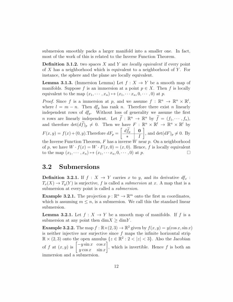
Definition 3.1.2. two spaces X and Y are locally equivalent if every pointof X has a neighborhood which is equivalent to a neighborhood of Y . Forinstance, the sphere and the plane are locally equivalent.

Lemma 3.1.3. (Immersion Lemma) Let f : X → Y be a smooth map ofmanifolds. Suppose f is an immersion at a point p ∈ X. Then f is locallyequivalent to the map (x1, · · · , xn) 7→ (x1, · · ·xn, 0, · · · , 0) at p.

Proof. Since f is a immersion at p, and we assume f : Rn → Rn × Rl,where l = m − n. Then dfp has rank n. Therefore there exist n linearlyindependent rows of dfp. Without loss of generality we assume the first

n rows are linearly independent. Let f̃ : Rn → Rn by f̃ = (f1, · · · , fn),

and therefore det(df̃)p 6= 0. Then we have F : Rn × Rl → Rn × Rl by

F (x, y) = f(x) +(0, y).Therefore dFp =

[df̃p 0∗ I

], and det(dF )p 6= 0. By

the Inverse Function Theorem, F has a inverse W near p. On a neighborhoodof p, we have W · f(x) = W · F (x, 0) = (x, 0). Hence, f is locally equivalentto the map (x1, · · · , xn) 7→ (x1, · · · xn, 0, · · · , 0) at p.

3.2 Submersions

Definition 3.2.1. If f : X → Y carries x to y, and its derivative dfx :Tx(X)→ Ty(Y ) is surjective, f is called a submersion at x. A map that is asubmersion at every point is called a submersion.

Example 3.2.1. The projection p : Rn → Rm onto the first m coordinates,which is assuming m ≤ n, is a submersion. We call this the standard linearsubmersion.

Lemma 3.2.1. Let f : X → Y be a smooth map of manifolds. If f is asubmersion at any point then dimX ≥ dimY .

Example 3.2.2. The map f : R×(2, 3)→ R2 given by f(x, y) = y(cosx, sinx)is neither injective nor surjective since f maps the infinite horizontal stripR × (2, 3) onto the open annulus {z ∈ R2 : 2 < |z| < 3}. Also the Jacobian

of f at (x, y) is

[−y sinx cosxy cosx sinx

], which is invertible. Hence f is both an

immersion and a submersion.

12

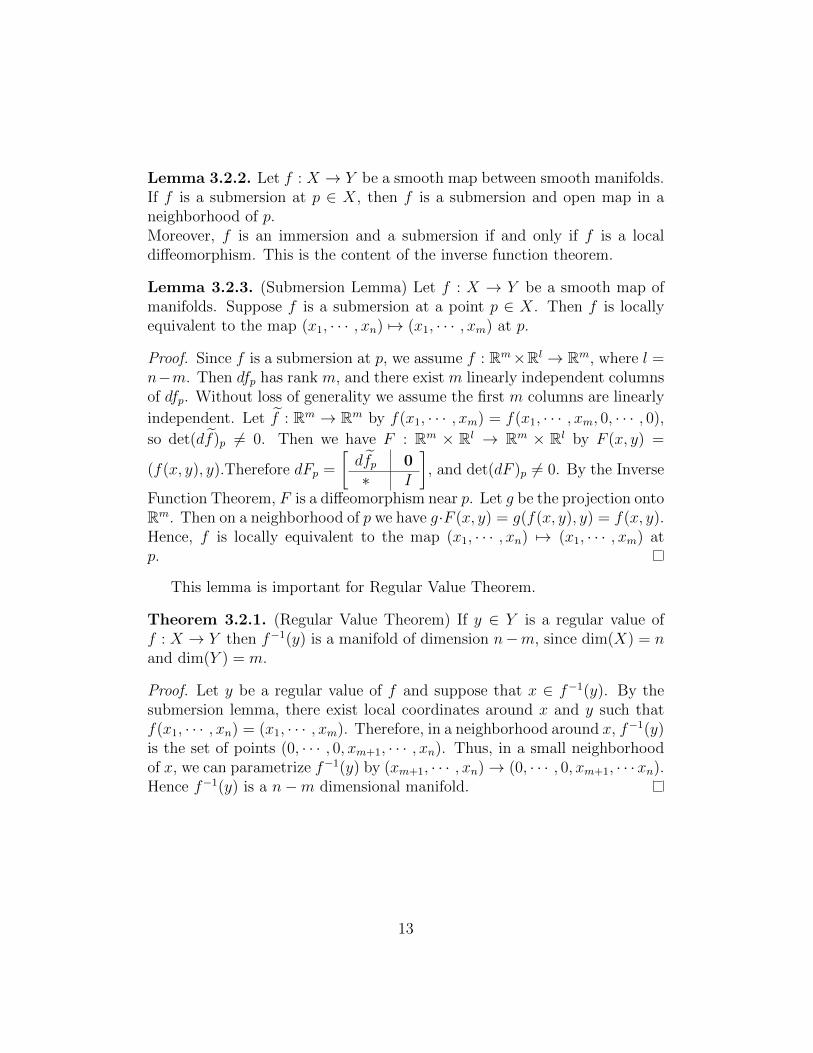
Lemma 3.2.2. Let f : X → Y be a smooth map between smooth manifolds.If f is a submersion at p ∈ X, then f is a submersion and open map in aneighborhood of p.Moreover, f is an immersion and a submersion if and only if f is a localdiffeomorphism. This is the content of the inverse function theorem.

Lemma 3.2.3. (Submersion Lemma) Let f : X → Y be a smooth map ofmanifolds. Suppose f is a submersion at a point p ∈ X. Then f is locallyequivalent to the map (x1, · · · , xn) 7→ (x1, · · · , xm) at p.

Proof. Since f is a submersion at p, we assume f : Rm×Rl → Rm, where l =n−m. Then dfp has rank m, and there exist m linearly independent columnsof dfp. Without loss of generality we assume the first m columns are linearly

independent. Let f̃ : Rm → Rm by f(x1, · · · , xm) = f(x1, · · · , xm, 0, · · · , 0),

so det(df̃)p 6= 0. Then we have F : Rm × Rl → Rm × Rl by F (x, y) =

(f(x, y), y).Therefore dFp =

[df̃p 0∗ I

], and det(dF )p 6= 0. By the Inverse

Function Theorem, F is a diffeomorphism near p. Let g be the projection ontoRm. Then on a neighborhood of p we have g·F (x, y) = g(f(x, y), y) = f(x, y).Hence, f is locally equivalent to the map (x1, · · · , xn) 7→ (x1, · · · , xm) atp.

This lemma is important for Regular Value Theorem.

Theorem 3.2.1. (Regular Value Theorem) If y ∈ Y is a regular value off : X → Y then f−1(y) is a manifold of dimension n−m, since dim(X) = nand dim(Y ) = m.

Proof. Let y be a regular value of f and suppose that x ∈ f−1(y). By thesubmersion lemma, there exist local coordinates around x and y such thatf(x1, · · · , xn) = (x1, · · · , xm). Therefore, in a neighborhood around x, f−1(y)is the set of points (0, · · · , 0, xm+1, · · · , xn). Thus, in a small neighborhoodof x, we can parametrize f−1(y) by (xm+1, · · · , xn)→ (0, · · · , 0, xm+1, · · ·xn).Hence f−1(y) is a n−m dimensional manifold.

13

Chapter 4

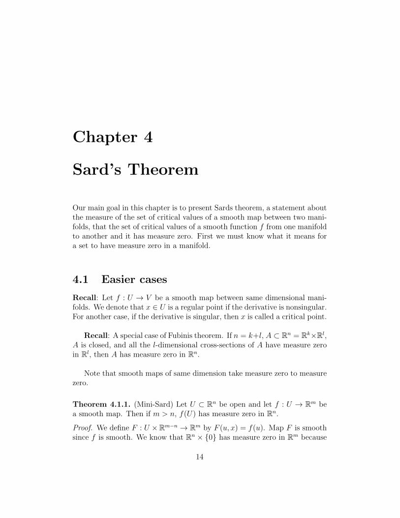
Sard’s Theorem

Our main goal in this chapter is to present Sards theorem, a statement aboutthe measure of the set of critical values of a smooth map between two mani-folds, that the set of critical values of a smooth function f from one manifoldto another and it has measure zero. First we must know what it means fora set to have measure zero in a manifold.

4.1 Easier cases

Recall: Let f : U → V be a smooth map between same dimensional mani-folds. We denote that x ∈ U is a regular point if the derivative is nonsingular.For another case, if the derivative is singular, then x is called a critical point.

Recall: A special case of Fubinis theorem. If n = k+l, A ⊂ Rn = Rk×Rl,A is closed, and all the l-dimensional cross-sections of A have measure zeroin Rl, then A has measure zero in Rn.

Note that smooth maps of same dimension take measure zero to measurezero.

Theorem 4.1.1. (Mini-Sard) Let U ⊂ Rn be open and let f : U → Rm bea smooth map. Then if m > n, f(U) has measure zero in Rn.

Proof. We define F : U ×Rm−n → Rm by F (u, x) = f(u). Map F is smoothsince f is smooth. We know that Rn × {0} has measure zero in Rm because

14

m > n, and therefore its subset U × {0} is also a set of measure zero inU × Rm−n. Thus F (U × {0}) has measure zero in Rm. Since F (U × {0}) =f(U), f(U) has measure zero in Rn.

Theorem 4.1.2. (Sard’s Theorem) Let f : X → Y be a smooth map ofmanifolds, and let C be the set of critical points of f in X. Then f(C) hasmeasure zero in Y .

Remark The theorem does not claim that the set of critical points in Xis a measure zero subset. In fact, if we consider a constant map, then anypoint in X is a critical point. However, f(X) is still a measure zero set, sinceany point not in f(X) is a regular value.

We begin with the easiest case in order to prove Sard’s Theorem, mapsof f : R1 → R1.

Theorem 4.1.3. Let U be an open set in R1, and f : U → R1 a continuouslydifferentiable map. Let C be the set of critical points of f such that C ={x ∈ U : f ′(x) = 0}. Then f(C) has measure zero in R1.

Proof. Let I be a closed interval inside U , and we define a function F : I×I →R1 by F (x, y) =

(f(y)− f(x)− f ′(x)(y − x))

|y − x|if x 6= y, and F (x, y) = 0

if x = y. Since f is continuously differentiable, the map F is uniformlycontinuous, and therefore F (x, y) can be made arbitrarily close to zero bymaking x and y sufficiently close to one another. Given any ε > 0, we candivide the interval I into n equal subintervals, each of length L

n, so that

|F (x, y)| < ε.Then we focus on any one of these subintervals which contains a critical pointx of f , so that f ′(x) = 0. Then for any other point y in that subinterval,we have |f(y)− f(x)− f ′(x)(y − x)| = |f(y)− f(x)| < ε|y − x| ≤ εL

n. Thus,

we have |f(y1)− f(y2)| ≤ 2εLn

, hence f contained in an interval with length≤ 2εL

n. There are at most n such subintervals, so the image under f of the

critical points which lie in the interval I is contained in a union of intervalsof total length 2εL, for ε > 0, and therefore has measure zero.Since the open set U is a countable union of such intervals I, it follows thatthe image under f of all the critical points also has measure zero. Hencef(C) has measure zero in R1.

15

Then we have the next case.

Theorem 4.1.4. Let U be an open set in R2, and f : U → R1 is a smoothmap. Let C be the set of critical points of f . Then f(C) has measure zeroin R1.

Proof. Since C is the set of critical points of f , let Ci ⊂ C be the set ofpoints x ∈ U where all partial derivatives of f of order ≤ i are zero. Thenwe have C ⊃ C1 ⊃ C2. We will prove it in three steps:step 1. The image f(C − C1) has measure zero.step 2. The image f(C1 − C2) has measure zero.step 3. The image f(C2) has measure zero.

proof of step 1.Since we have C ⊃ C1 ⊃ C2, and therefore C − C1 is singular but non-zeroJacobian. Hence the image f(C − C1) has measure zero, completing step 1.

proof of step 2.For each point x∗ in C1−C2, there is ∂2f

∂xi∂xjwhich is not zero at x∗. Therefore

the function g(x) = ∂f∂xj

vanishes at x∗. but ∂g∂xi

= ∂2f∂xi∂xj

does not. Without

lose of generality, we assume i = 1, and we define a map h : U → R2 byh(x) = (g(x), x2). The Jacobian matrix dh is nonsingular, so h carries someneighborhood V of x∗ diffeomorphically onto an open set V ′ in R2.h carries C1 ∩V into 0×R1, and now we consider the function w = f ◦ h−1 :V ′ → R1, and let w∗ : (0 × R1) ∩ V ′ → R1. Hence, the set of critical valuesof w∗ has measure zero in R1.But each point in h(C1 ∩ V ) is certainly a critical point of w∗, since all firstorder derivatives vanish at such points. Therefore w∗◦h(C1∩V ) = f(C1∩V )has measure zero. Since C1 − C2 is covered by countably many such sets V ,it follows that f(C1 − C2) has measure zero, completing step 2.

proof of step 3. (This is similar to the proof for R1)Let I be a closed square inside U with edge length L. We will show thatf(C2 ∩U) has measure zero. By Taylors Theorem, the compactness of I, wehave that f(x + h) = f(x) + R(x, h) with |R(x, h)| ≤ a|h|3 for x ∈ C2 ∩ Iand x + h ∈ I, where the constant a depends only on f and I. Then wesubdivide I into n2 subsquares, each of side length L

n. Let S be a square of

16

this subdivision which contains a point of Ck.Then any point of S can be written as x + h, with |h| ≤

√2Ln

. Therefore

it follows that f(S) must lie in an interval of length 2a(√

2Ln

)3 centered atf(x). There are at most n2such subsquares S, hence f(C2 ∩ I) is containedin a union of intervals of total length at most n22a(

√2Ln

)3 = b/n, for someconstant b.This total length tends to 0 as n→∞, so f(C2∩ I)have measure zero. SinceU can be covered with countably many such squares, this shows that f(C2)has measure zero, completing step 3.Hence, f(C) has measure zero in R1.

We already begin to see general case in two dimensional example, and weprove in three steps. Fisrt, we show that the image f(C − C1) has measurezero, and then we show the image f(C1 − C2) has measure zero, finally weshow the image f(C2) has measure zero.

4.2 Proof of Sard’s theorem

Therefore we have

Theorem 4.2.1. (Sard’s theorem) Let U be an open set in Rn, and f : U →Rp is a smooth map. Let C be the set of critical points of f . Then f(C) hasmeasure zero in Rp.

The theorem is certainly true for n = 0. We will proceed to provethat the theorem is true for n assuming that it is true for n − 1. DenoteC1 := {x ∈ U : (df)x = 0}, and for i ≥ 1, we have Ci := {x ∈ U : allpartial derivatives of f of order ≤ i vanish at x}. Notice that each Ci is builtby taking a finite intersection of sets, and each Ci is closed, so we have adescending sequence of closed sets C ⊃ C1 ⊃ C2 ⊃ · · · . We then proceed byinduction and prove three lemmas.

we will divide the proof into three steps:step 1. f(Ck) has measure zero for k ≥ n/p− 1.step 2. f(Ck − Ck+1) has measure zero.step 3. f(C − C1) has measure zero.

17

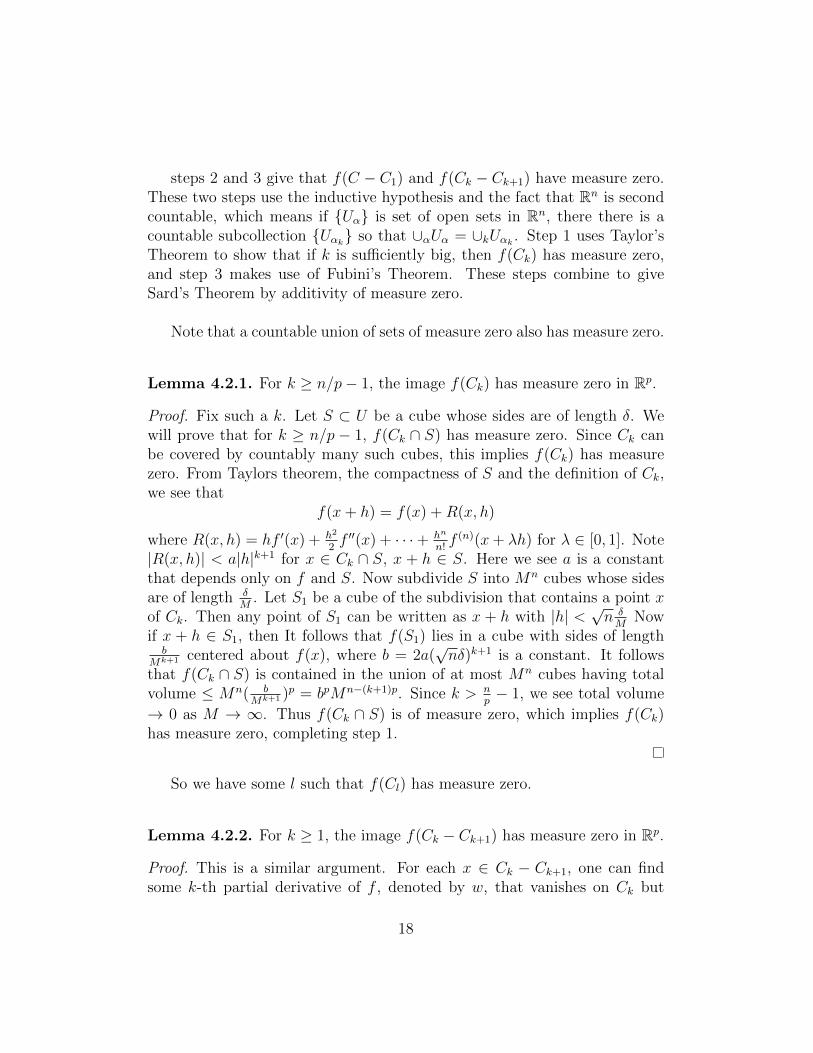
steps 2 and 3 give that f(C − C1) and f(Ck − Ck+1) have measure zero.These two steps use the inductive hypothesis and the fact that Rn is secondcountable, which means if {Uα} is set of open sets in Rn, there there is acountable subcollection {Uαk

} so that ∪αUα = ∪kUαk. Step 1 uses Taylor’s

Theorem to show that if k is sufficiently big, then f(Ck) has measure zero,and step 3 makes use of Fubini’s Theorem. These steps combine to giveSard’s Theorem by additivity of measure zero.

Note that a countable union of sets of measure zero also has measure zero.

Lemma 4.2.1. For k ≥ n/p− 1, the image f(Ck) has measure zero in Rp.

Proof. Fix such a k. Let S ⊂ U be a cube whose sides are of length δ. Wewill prove that for k ≥ n/p − 1, f(Ck ∩ S) has measure zero. Since Ck canbe covered by countably many such cubes, this implies f(Ck) has measurezero. From Taylors theorem, the compactness of S and the definition of Ck,we see that

f(x+ h) = f(x) +R(x, h)

where R(x, h) = hf ′(x) + h2

2f ′′(x) + · · ·+ hn

n!f (n)(x+ λh) for λ ∈ [0, 1]. Note

|R(x, h)| < a|h|k+1 for x ∈ Ck ∩ S, x + h ∈ S. Here we see a is a constantthat depends only on f and S. Now subdivide S into Mn cubes whose sidesare of length δ

M. Let S1 be a cube of the subdivision that contains a point x

of Ck. Then any point of S1 can be written as x + h with |h| <√n δM

Nowif x + h ∈ S1, then It follows that f(S1) lies in a cube with sides of lengthb

Mk+1 centered about f(x), where b = 2a(√nδ)k+1 is a constant. It follows

that f(Ck ∩ S) is contained in the union of at most Mn cubes having totalvolume ≤ Mn( b

Mk+1 )p = bpMn−(k+1)p. Since k > np− 1, we see total volume

→ 0 as M → ∞. Thus f(Ck ∩ S) is of measure zero, which implies f(Ck)has measure zero, completing step 1.

So we have some l such that f(Cl) has measure zero.

Lemma 4.2.2. For k ≥ 1, the image f(Ck − Ck+1) has measure zero in Rp.

Proof. This is a similar argument. For each x ∈ Ck − Ck+1, one can findsome k-th partial derivative of f , denoted by w, that vanishes on Ck but

18

has a first derivative, ∂w∂x1

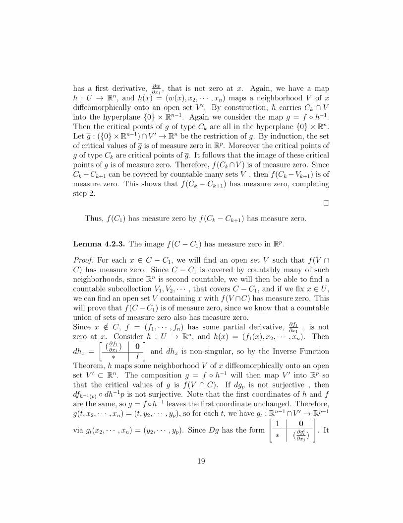
, that is not zero at x. Again, we have a maph : U → Rn, and h(x) = (w(x), x2, · · · , xn) maps a neighborhood V of xdiffeomorphically onto an open set V ′. By construction, h carries Ck ∩ Vinto the hyperplane {0} × Rn−1. Again we consider the map g = f ◦ h−1.Then the critical points of g of type Ck are all in the hyperplane {0} × Rn.Let g : ({0}×Rn−1)∩V ′ → Rn be the restriction of g. By induction, the setof critical values of g is of measure zero in Rp. Moreover the critical points ofg of type Ck are critical points of g. It follows that the image of these criticalpoints of g is of measure zero. Therefore, f(Ck∩V ) is of measure zero. SinceCk−Ck+1 can be covered by countable many sets V , then f(Ck−Vk+1) is ofmeasure zero. This shows that f(Ck − Ck+1) has measure zero, completingstep 2.

Thus, f(C1) has measure zero by f(Ck − Ck+1) has measure zero.

Lemma 4.2.3. The image f(C − C1) has measure zero in Rp.

Proof. For each x ∈ C − C1, we will find an open set V such that f(V ∩C) has measure zero. Since C − C1 is covered by countably many of suchneighborhoods, since Rn is second countable, we will then be able to find acountable subcollection V1, V2, · · · , that covers C − C1, and if we fix x ∈ U ,we can find an open set V containing x with f(V ∩C) has measure zero. Thiswill prove that f(C−C1) is of measure zero, since we know that a countableunion of sets of measure zero also has measure zero.Since x /∈ C, f = (f1, · · · , fn) has some partial derivative, ∂f1

∂x1, is not

zero at x. Consider h : U → Rn, and h(x) = (f1(x), x2, · · · , xn). Then

dhx =

[( ∂f1∂x1

) 0

∗ I

]and dhx is non-singular, so by the Inverse Function

Theorem, h maps some neighborhood V of x diffeomorphically onto an openset V ′ ⊂ Rn. The composition g = f ◦ h−1 will then map V ′ into Rp sothat the critical values of g is f(V ∩ C). If dgp is not surjective , thendfh−1(p) ◦ dh−1p is not surjective. Note that the first coordinates of h and fare the same, so g = f ◦h−1 leaves the first coordinate unchanged. Therefore,g(t, x2, · · · , xn) = (t, y2, · · · , yp), so for each t, we have gt : Rn−1∩V ′ → Rp−1

via gt(x2, · · · , xn) = (y2, · · · , yp). Since Dg has the form

[1 0

∗ (∂gti∂xj

)

]. It

19

follows that a point p ∈ Rn−1 is critical for gt if and only if {t}× p is criticalfor g.By induction, Sards theorem is true for n − 1, so the set of critical valuesof gt has measure zero. Finally applying Fubinis theorem, we see that theset of critical values of g is of measure zero. this shows that f(C − C1) hasmeasure zero, completing step 3.

Hence, we get that f(C) has measure zero.

4.3 Examples

Here are some examples.

Example 4.3.1. If X is a manifold, then the identity mapping f : X → Xhas no critical points, and therefore the set of nonregular values has measurezero.

Example 4.3.2. Let f : R2 → R, and f(x, y) = x2 + y2 is given. We havethe derivative zero only at the origin, and f(0, 0) is just a single point, whichhas measure zero in R.

Lemma 4.3.1. If a set A ⊆ Rn has measure zero, then its complement isdense.

Proof. If U is any nonempty open set in Rn, then it intersect the complementof A, otherwise it will lie completely in A. Therefore U also has measure zeroas would any cube C in U , but if C has side δ, its measure δn is positive.Hence the complement of A is dense.

Corollary 4.3.1. Let f : X → Y be a smooth map of manifolds. Then theregular values of f form a dense subset of Y .

Proof. The set of critical values of f is closed and has measure zero, andtherefore the set of regular values of f , which is the complement of the setof critical values of f in Y , and hence is dense in Y .

20

Chapter 5

Applications of Sard’s Theorem

This chapter we will discuss the applications of Sard’s Theorem, such asapplications to the Whitney Embedding and Immersion Theorems, the exis-tence of Morse functions, and Brouwer’s fixed point theorem.

Sard’s Theorem Let f : X → Y be a smooth map of manifolds, andlet C be the set of critical points of f in X. Then f(C) has measure zero in Y .

Regular Value Theorem If y is a regular value of f : X → Y , then thepreimage f−1(y) is a submanifold of X, with dim f−1(y) = dimX − dimY .

Sard’s theorem is important, since combining the Preimage Theorem withSard’s Theorem, we know that since almost all values of a mapping are regu-lar, the preimage of a mapping is almost always a manifold. There are manyother useful results which rely on Sard’s Theorem, such as the Whitney Em-bedding Theorem, the Whitney Immersion Theorem, the existence of Morsefunctions, and the Brouwer’s fixed point theorem.

5.1 Whitney Embedding Theorem

Let M be a smooth manifold of dimension n. A natural question is: whichmaniolds can be embedded into Rm as smooth submanifolds? We proceed toour first application.

21

Theorem 5.1.1. Any smooth manifold Mn ⊂ Rm has an injective immer-sion into R2n+1.

Proof. Suppose i : M → Rm embedding πa ◦ i : M → Va⊥ ∼= Rm−1. Ifm = 2n + 1, we are done, so we assume m > 2n + 1. For a ∈ Rm such thata 6= 0, the projection proja⊥v = v − ( v·a

a·a)a. Let πa be the projection of Rm

to the normal, and it suffices to show that πa|M : M → Rm−1 is an injectiveimmersion for at least one a. We will use Sard’s Theorem to show that itis true. Define g : M ×M × R → Rm, and g(x, y, t) = t(x − y), also defineh : TM → Rm with h(p, v) = (di)p(v), where (p, v) ∈ TM represents thetangent vector v ∈ Rm at the point p ∈M , and dip : TMp → TRm

i(p) = Rm. If

πa : M → Rm−1 is not injective, then we have some x, y ∈M , s ∈ R such thatx 6= y and x − y = sa. Therefore, g(x, y, 1/s) = 1/s(x − y) = 1/s(sa) = a.Furthermore, if πa is not an immersion, then d(πa ◦ i)pv = 0 = πa ◦ dip(v)where πa is the projection of Rm and dip(v) is a vector in Rm, and thus thereis some (p, v) ∈ TM such that dip(v) = s ·a for some a. Since M is immersedinto Rm, we must have s 6= 0, so h(v/s) = a. Now it is clear that if a is inneither the range of g or the range of h, then πa is the injective immersion.Since the dimensions of the domains of g and h are 2n+1 and 2n respectively,and m > 2n+1, every point in the range of these functions is a critical value.Thus we can pick almost any a ∈ Rm and get that πa : M → Rm−1 is aninjective immersion.

Note that if M is compact, then an injective immersion is an embedding,so this theorem comes very close to the weak Whitney Embedding Theorem,every manifold Mn can be embedded into R2n.

Theorem 5.1.2. (Abstract Whitney) A smooth manifold Mn embeds in RN

for some large N .

There is a proof in “Introduction to Smooth Manifolds” by Lee, John M.

5.2 Morse Functions

Our next application of Sard’s Theorem will be the existence of Morse func-tions.

22

Given a function f : M → R, a critical point x ∈ M is called non-degenerate if the Hessian matrix H of f at x, H(f)x = ( ∂2f

∂xi∂xj) is nonsin-

gular, and functions are important because f is locally quadratic at thesecritical points. If all of f ’s critical points are non-degenerate, f is called aMorse function. Morse functions say a great deal about the topology of M .

Definition 5.2.1. If H(f)x is non-singular at the critical point x ∈ M , wesay that x is a non-degenerate critical point of f .

Note that the non-degenerate critical points are isolated, because criticalpoints are the zeros of the function g = ( ∂f

∂x1+ · · ·+ ∂f

∂xn). Thus H(f)x = dgx,

so if H(f)x is non-singular, the inverse function theorem tells us that g hasa local inverse, hence g has no other zeros in some neighborhood of x.

Definition 5.2.2. A function f : M → R such that all its critical points arenon-degenerate is called a Morse function.

Example 5.2.1. Morse functions are useful in topology. For instance, atorus T 2 in R3 on its rim in the xy-plane and define the height functionh : T 2 → R by h(x, y, z) = z for (x, y, z) ∈ T 2. Then h is a Morse function.It has four critical points: a minimum at two saddle points, and a maximum.

Theorem 5.2.1. There are lots of Morse functions: given M ⊂ Rn, andf : M → R, then fa = f + a1x1 + · · · + anxn is a Morse function for almostevery a ∈ Rn.

Proof. Define g = df = ( ∂f∂x1

+ · · · + ∂f∂xn

) on M . Note that dfa = g + a, andH(fa) = H(f) = dg. Pick any a so that −a is a regular value for g. Then if xis a critical point of fa, we have g(x) = −a, and for (d(fa))x : TMx → R, andif not surjective, then it is zero. Therefore (dfa)x = g+a = 0, so H(fa)x = dgxis nonsingular. Hence fa is a Morse function.

5.3 Brouwer’s Fixed Point Theorem

The next application of Sard’s Theorem will be the Brouwer’s fixed pointtheorem.

23

A fixed point of a function f : X → X is a point x0 such that f(x0) = x0.

Example 5.3.1. The intermediate value theorem implies that every contin-uous function f : [−1, 1]→ [−1, 1] has a fixed point.

Proof. We have f : [−1, 1]→ [−1, 1]. Define g(x) = x−f(x). Then g(1) ≥ 0and g(−1) ≤ 0 so by the Intermediate Value Theorem there must be a pointx0 so that g(x0) = 0. We then have f(x0) = x0.

Theorems which establish the existence of fixed points are very useful inanalysis. One of the most famous is due to Brouwer. Let Dn = {x ∈ R :|x| ≤ 1}.

Recall the Weierstrass Approximation Theorem.

Theorem 5.3.1. (Weierstrass Approximation Theorem.) Let f ∈ C[a, b].Given any ε > 0 there exists a polynomial pn of sufficiently high degree n forwhich |f(x)− pn(x)| ≤ ε for all x ∈ [a, b].

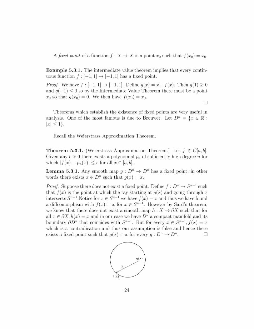
Lemma 5.3.1. Any smooth map g : Dn → Dn has a fixed point, in otherwords there exists x ∈ Dn such that g(x) = x.

Proof. Suppose there does not exist a fixed point. Define f : Dn → Sn−1 suchthat f(x) is the point at which the ray starting at g(x) and going through xintersects Sn−1.Notice for x ∈ Sn−1 we have f(x) = x and thus we have founda diffeomorphism with f(x) = x for x ∈ Sn−1. However by Sard’s theorem,we know that there does not exist a smooth map h : X → ∂X such that forall x ∈ ∂X, h(x) = x and in our case we have Dn a compact manifold and itsboundary ∂Dn that coincides with Sn−1. But for every x ∈ Sn−1, f(x) = xwhich is a contradication and thus our assumption is false and hence thereexists a fixed point such that g(x) = x for every g : Dn → Dn.

24

Theorem 5.3.2. (Brouwers Fixed Point Theorem.) Every continuous func-tion f : Dn → Dn has a fixed point, in other words there exists x ∈ Dn suchthat f(x) = x.

Proof. Approximate f by a smooth mapping. Given ε > 0, according tothe Weierstrass approximation theorem, there is a polynomial function p1 :Rn → Rn with |p1(x) − f(x)| < ε for x ∈ Dn. However, p1 may send points

of Dn into points outside of Dn. Then we let p(x) = p1(x)1+ε

, so p maps Dn

into itself and |p(x)− f(x)| < 2ε for x ∈ Dn. Suppose that f(x) 6= x for allx ∈ Dn. Then the continuous function |f(x) − x| must take on a minimumµ > 0 on Dn. Let p : Dn → Dn with |p(x) − f(x)| < µ for all x, we clearlyhave p(x) 6= x. Thus p is a smooth map from Dn to itself without a fixedpoint. This contradicts Lemma, and hence has a fixed point.

25

Chapter 6

S2 is simply connected

After the Brouwers Fixed Point Theorem, we will also use polynomial ap-proximation to prove S2 is simply connected, since any smooth map of acircle must miss a point, so we will develop this with mention of polynomialapproximation to give a full proof of the topological case.

6.1 Definitions

We define that a nonempty space X is said to be simply connected if it ispath-connected and has trivial fundamental group.

Definition 6.1.1. X is path-connected if for every p, q ∈ X, there exists acontinuous map γ : [0, 1]→ X such that γ(0) = p and γ(1) = q. The map γis called a path connecting p and q.

Definition 6.1.2. For a space X and a fixed point x0 ∈ X, The set ofhomotopy classes of loops based at x0, is called the fundamental group of Xrelative to the base point x0. We denote this group by π1(X, x0).

Example 6.1.1. The fundamental group of the closed unit disk D2, i.e.π1(D

2, x0) where x0 is any point in D2, is trivial.

Since any two points in D2 are path connected, without loss of generality,we can pick x0 = (0, 0). Then for any loop f based at x0, the following mapF : [0, 1] × [0, 1] → D2 given by F (x, t) = (1 − t)f(x) is a path homotopybetween f and the constant map. Therefore there is only one element inπ1(D

2, x0). Hence π1(D2, x0) is trivial.

26

6.2 Proof of S2 is simply connected

We will prove that S2 is simply connected, and recall S2 = {(x, y, z) ∈R3|x2 + y2 + z2 = 1}.

Proposition 6.2.1. Suppose U and V are open sets in X and X = U ∪ V ,and U∩V is nonempty and path connected. If U and V are simply connected,then X is simply connected.

Proof. Since U and V are simply connected, π1(U, x0) and π1(V, x0) are triv-ial. The homomorphisms induced by the inclusion maps take the identitiesof these two groups to the identity of the fundamental group π1(X, x0). Butsince the images of π1(U, x0) and π1(V, x0) generate π1(X, x0), so π1(X, x0)is trivial, by Van Kampen theorem. Hence X is simply connected.

We will show two proofs, one is using the Van Kampen theorem which isno differentiable topology, and the other one is by using the Sard’s theorem.

Theorem 6.2.2. S2 is simply connected.

Proof. (by Van Kampen theorem )Let a = (0, 0, 1) be the “north pole” of the sphere S2. Consider the setU = S2 \ a and we claim that U is simply connected. Define P : U → R2 bythe equation

P (x, y, z) = (x

1− z,

y

1− z)

One can verify that P is a homeomorphism and its inverse is given by theequation

P−1(x, y) = (2x

1 + x2 + y2,

2y

1 + x2 + y2,−1 + x2 + y2

1 + x2 + y2)

Therefore the fundamental group of U is isomorphic to the fundamentalgroup of R2, which is trivial. Similarly, if b = (0, 0,−1) is the “south pole”of S2, then the fundamental group of the space V = S2 \ b is also trivial.We know that U ∩V is not empty, and moreover we claim that U ∩V is pathconnected. This is because the map P is a homeomorphism between U ∩ Vand R2 \ {0}. For two points c and d in U ∩ V , P (c) and P (d) can be jointby a path g in R2 \{0} since R2 \{0} is path connected. This implies c and dcan be joint by the path P−1(g) in U ∩ V . Hence we can apply the corollaryabove and conclude that S2 is simply connected.

27

Proof. (by Sard’s theorem) Let f : S1 → S2 be a smooth map. We wouldlike to show that this is nulhomotopic. By Sards theorem, we know thatany smooth map f : S1 → S2 misses a point, and therefore we choosep ∈ S2 \ f(S1). Then we have S2 \ {p} is simply connected. Thus f(S1) isdiffeomorphic to a loop in R2, which is homotopic to a constant. Thereforethis homotopy can be pulled back along the diffeomorphism, so f(S1) issimply connected in S2 \ {p}, and thus in S2 as well. Hence S2 is simplyconnected.

Moreover, in fact, Sn is simply connected for n ≥ 2.

28

Chapter 7

Future Work

We have proved the Whitney Embedding Theorem: Any smooth manifoldMn ⊂ Rm has an injective immersion into R2n+1 by using Sard’s Theoremand Regular Value Theorem, and for future work, there is a hard versionWhitney Theorem: Any smooth manifold Mn embeds in R2n, immerses inR2n−1. We can show that there are manifolds Mn that do not embed in Rk

for k < 2n by algebraic topology.

29

Bibliography

[1] Kosinski, Antoni A. Differential Manifolds. Mineola, NY: Dover Publica-tions, 2007.

[2] Milnor, John W. Topology from the Differentiable Viewpoint. Princeton,NJ: Princeton UP, 1997.

[3] Guillemin, Victor, and Alan Pollack. Differential Topology. Providence,RI: AMS Chelsea Pub., 2010.

[4] Tu, Loring W. An Introduction to Manifolds. 2nd ed. New York: Springer,2011.

[5] Lee, John M. Introduction to Smooth Manifolds. New York: Springer,2006.

[6] Chan, Henry Y. Measure Zero The Student Mathematical Library Wind-ing Around, 2013. PDF file.

[7] Wang, Zuoqin Lecture 9: Sards Theorem 2009. PDF file.

[8] Pflueger, Nathan Math 1B, lecture 14: Taylors Theorem 2011. PDF file.

[9] Alfeld, Peter The Weierstrass Approximation Theorem 2013. PDF file.

[10] Blair, Ryan Math 600 Day 5: Sards Theorem 2010. PDF file.

[11] Weng, Daping Invariance of domain and the jordan curve theorem inR2 2009. PDF file.

[12] Caratelli, Daniele Brouwers Fixed Point Theorem 2012. PDF file.

[13] McCain, William C. Sard & Whitney 2005. PDF file.

30

[14] Bloom, Jonathan Michael The Local Sturcture of Smooth Maps of Man-ifolds 2004. PDF file.

31