i

SAS Institute Pre-sales Internship

Bruno Alexandre Zeverino António

Internship Report

Internship report presented as partial requirement for

obtaining the Master’s degree in Advanced Analytics

ii

NOVA Information Management School

Instituto Superior de Estatística e Gestão de Informação

Universidade Nova de Lisboa

INTERNSHIP REPORT

by

Bruno António

Internship report presented as partial requirement for obtaining the Master’s degree in Advanced

Analytics

Co Advisor: Miguel de Castro Neto

Co Advisor: Simone da Costa Sousa

November 2016

iii

ABSTRACT

The present document describes the work developed during the six months internship at SAS®

Institute Inc.. During the internship, the intern provided support to the Pre-Sales department by

integrating the analytic team. The intern received access to an extensive selection of courses

designed to introduce the core technologies and present the analytical tools developed by SAS®. He

was later integrated in a team working in a proof of concept dedicated to showcase the forecast

capability of SAS® Forecast Server in the beverage industry.

KEYWORDS

Forecast; Demand Planning; SAS® Forecast Server

SAS Institute Inc., SAS Campus Drive, Cary, North Carolina 27513.

SAS® and all other SAS Institute Inc. product or service names are registered trademarks or

trademarks of SAS Institute Inc. in the USA and other countries. ® indicates USA registration.

iv

INDEX

1. Introduction .................................................................................................................. 1

2. Forecasting ................................................................................................................... 2

3. Proof of concept objective ........................................................................................... 3

4. Data............................................................................................................................... 5

5. SAS® Forecast Server .................................................................................................... 6

5.1. Data requirements ................................................................................................ 6

5.2. Hierarchy ............................................................................................................... 6

5.3. Variables’ roles ...................................................................................................... 6

5.4. Missing data........................................................................................................... 7

5.5. Forecast periods .................................................................................................... 7

5.6. Modelling ............................................................................................................... 7

6. Time requirements and interpolation .......................................................................... 9

6.1. Monthly to Weekly Interpolation .......................................................................... 9

7. Results Comparison .................................................................................................... 14

8. Results......................................................................................................................... 17

8.1. Results for Weekly Data ...................................................................................... 17

8.2. Results for Monthly Data ..................................................................................... 18

8.3. Discussion of Results ........................................................................................... 20

9. Conclusions ................................................................................................................. 21

10. Bibliography.......................................................................................................... 22

11. Annexes ................................................................................................................ 23

v

LIST OF FIGURES

Figure 1: Schema of the process followed during the PoC …………………………………………………………………4

Figure 2: Forecasting view in SAS® FS ……………………………………………………………………………………...…....…8

Figure 3: Monthly forecasts used by the interpolation methods to obtain weekly forecasts.........……11

Figure 4: Forecasts obtained by interpolating the data from Figure 2 using the spline method ……….12

Figure 5: Forecasts obtained by interpolating the data from Figure 2 using the join method …………..12

Figure 6: Forecasts obtained by interpolating the data from Figure 2 using the step method ………….13

Figure 7: Scatter plot of CA vs MAPA for 45 forecast series ……………………………………………………………..16

vi

LIST OF TABLES

Table 1: Conditions of the forecast ……………………………………………..…………………………………………………….4

Table 2: Original format of the data …………………………………………………………………………………………………10

Table 3: PROC EXPAND compatible data format ………………………………………………………………………………10

Table 4: Weekly forecasts results comparison in absence and presence of holdout sample …………….18

Table 5: Interpolation methods’ results comparison for monthly data …………………………………………….19

vii

LIST OF ABBREVIATIONS AND ACRONYMS

SAS® FS SAS® Forecast Server. Software developed to provide a simple user-interface dedicated

to forecast time series.

SAS® VA SAS® Visual Analytics

PoC Proof of Concept

1

1. INTRODUCTION

The present document describes the work developed during the six months internship at SAS

Institute Inc.. The internship is a result of the cooperation between the Nova IMS and SAS Institute

Inc. with the goal of catalyzing the transition of students to the workforce. During the internship, the

intern provided support to the Pre-Sales department by integrating the analytic team. This team is

responsible for demonstrating the SAS® products’ capabilities to prospect clients, ranging from

solutions dedicated to specific industries such as banking, insurance and manufacturing to more

flexible products that can be used in a variety of contexts. It is formed by individuals with distinct

areas of expertise such as information management, insurance and even physical sciences that work

together to highlight the products’ features that can help customers improve their businesses.

The intern received access to an extensive selection of courses designed to introduce the core

technologies and present the analytical tools developed by SAS® as it is crucial that the intern has a

firm grasp of the SAS® technology. The courses covered the SAS® language and data manipulation

techniques and several SAS® products. Additionally, the SAS® data visualization products SAS® Visual

Analytics and SAS® Visual Statistics were explored. VS allows the user to intuitively use the available

data to tell a story that is easily understandable and visually appealing.

The intern was later integrated in a team working in a proof of concept dedicated to showcase the

forecast capability of SAS® Forecast Server in the beverage industry. The PoC (Proof of Concept) was

requested by the prospect to compare the capability of SAS® FS to the solution currently used that

was provided by another company. The main issues with the implemented software for forecasting is

that it is not flexible enough to be applied to new situations without external consulting and it does

not possess sophisticated models required to model complex series. Although the current software

has forecast capabilities, it was not specifically developed to produce forecasts. For this reason it

misses key features that may undermine the prospect’s ability to be proactive in their strategy.

2

2. FORECASTING

Forecasting has been used since ancient times as a survival tool. Used to improve crops’ yielding and

to prepare for battles, such in the infamous Battle of Waterloo and the D-Day, it often relied in

superstitions, astronomical observations or weather pattern recognition.1-8

In the digital age, however, we are no longer bound to the usage of unfounded and primitive forms

of forecasting. We have available centuries of mathematical knowledge that empowers us to be able

to make the decisions based on documented statistical methods. Such methods are used for more

than just predicting weather. Application range from stock trading, customer demand planning,

supply chain management and even sports betting. 9

Time series is a series of discrete data points ordered in time. In most cases, the data points is equally

spaced in time. Times series can be used to develop models to predict the values of the series in the

future according to previous observations. Time series models are usually used when reduced

information is available about the variables at play, when the number of data points is large and

when the models are to be used to forecast in small time periods. 10

3

3. PROOF OF CONCEPT OBJECTIVE

Companies are in a constant struggle to remain competitive. It is not uncommon for companies to

bankrupt because they did not adapt to a changing playing field. Marketing campaigns, price

optimization and production waste reduction are some of several strategies are devised and apply to

gain advantage over competitors. The company in contact with the Pre-sales team intends to swift

from a production-based company to a demand-based company. As with most corporative

transitions, it requires additional efforts in terms of replacing or updating technology and changing

the administration mind-set. One of the step to achieve demand-based operations is to measure,

analyze and predict demand. While the prospect already collects data regarding the sales of its

beverages it still does not use this data to improve its processes. It is quintessential to predict the

sales in the upcoming weeks as the period between production and distribution can take several

weeks. The objective of the prospect is to acquire a product that enables the production department

to have a clear notion of the amount of beverages that need to be produce at any given time. The

product has to be simple to use, scalable and the result have to be able to be used by several

departments. With this in mind the pre-sales analytics team set up to promote SAS® Forecast Server

as a tool to achieve the wanted goal. The chosen approach was to prepare a proof-of-concept to

highlight the capability of SAS® Forecast Server to tackle the prospect’s issues.

One might think that gathering the data, preparing the forecasts and show the results would be

enough to persuade a potential client. Generally this is not case as a continuous communication with

the prospect is require to make sure that the expectations are aligned. It is necessary to understand

the business model and how the forecast results are directly applied to the business. The process is

summarized in table 1 where it is clear that theoretical analysis are insufficient if the remaining steps

are ignored.

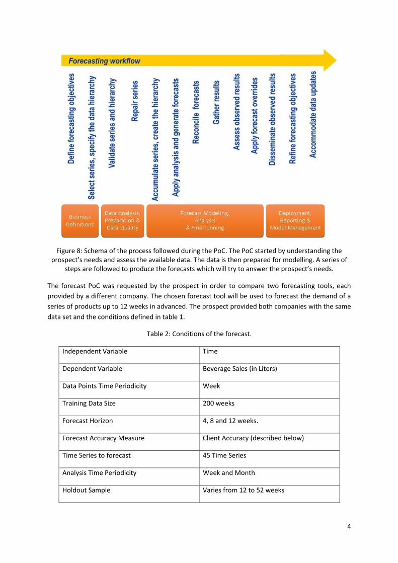
4

Figure 8: Schema of the process followed during the PoC. The PoC started by understanding the prospect’s needs and assess the available data. The data is then prepared for modelling. A series of

steps are followed to produce the forecasts which will try to answer the prospect’s needs.

The forecast PoC was requested by the prospect in order to compare two forecasting tools, each

provided by a different company. The chosen forecast tool will be used to forecast the demand of a

series of products up to 12 weeks in advanced. The prospect provided both companies with the same

data set and the conditions defined in table 1.

Table 2: Conditions of the forecast.

Independent Variable Time

Dependent Variable Beverage Sales (in Liters)

Data Points Time Periodicity Week

Training Data Size 200 weeks

Forecast Horizon 4, 8 and 12 weeks.

Forecast Accuracy Measure Client Accuracy (described below)

Time Series to forecast 45 Time Series

Analysis Time Periodicity Week and Month

Holdout Sample Varies from 12 to 52 weeks

5

4. DATA

The original data sent by the prospect has the following proprieties:

1 ID variable that identifies each products.

16 categorical variables about the product such as brand, flavor, size package that categorize

the products.

8 point of sale variables: region, manager ID, sales strategy and others.

5 date variables: date, year, month, week, first day of the month and first day of the week.

The weeks are considered to start on Sundays and are identified by that day.

Quantity sold: represents the balance between the amount sold and the amount returned to

the company inventory, in liters. Positive values indicate that the sales were superior to the

returns. Negative values indicate that the returns were superior to the sales. Most weeks the

balance is positive but can occasionally be negative.

As described before, the scope of the PoC is to produce forecasts and compare them with the ones

obtained by the competitor. To do so, the input data must be exactly the same as used by the

competitor. This required a dimension reduction operation to be performed to remove 16

categorical variables. After the removal of the categorical variables the data was aggregated as need.

For instance, the sales of the same product from different managers have to be summed together as

only the overall sales matter to the forecast. The resulting data set has the following variables:

Cluster: an ID variable that identifies each product. The cluster variable distinguishes

different beverages but also different packages materials and sizes for the same beverage.

Group_GAOV: a variable used to indicate the region where the product was sold. It can

indicate a country if the product was sold abroad or the kind of seller if it was sold within the

country.

Sales Amount: Amount of liters of beverage sold per week.

Date: a variable that indicates the date of the first day of the week.

Even though SAS® FS can perform some data preparation, it is not an ETL tool. SAS® Enterprise Guide

was used instead to process the data and prepare it for forecast as it has available more flexible data

manipulation options.

There is an intermediate phase between data preparation and forecast that focus on studying how

the overall time series behaves. The analysis of volatilities can be used to manage the prospect’s

expectations about the results that can be achieved but also to verify which series can be forecasted

and which do not meet the requirements necessary to produce meaningful forecasts.

6

5. SAS® FORECAST SERVER

After preparing the data, it was imported to SAS® FS, a software developed by SAS® Institute Inc.11

which provides a powerful Graphical User Interface (GUI) that automates the forecasting process.

The prospect requested the forecasts to be performed without using advanced techniques or

settings that could not be easily taught to an employee with no programming or statistical

background. Forecast Server is a perfect tool to be used for this purpose because it is ready to use

and with no need to code the forecast models. In order to follow the prospect’s requirements, only

the general settings were changed. These settings changes are straightforward and can be taught in a

one-day course.

The import procedure is simple and acts as a data quality control. Any issue with the data that would

prevent the software from producing forecasts needs to be fixed before proceeding. The following

section describe some of the settings that are defined during the import process.

5.1. DATA REQUIREMENTS

In order to use SAS® FS certain requirements must be fulfilled.

The data set must contain a time ID variable that identifies the time period for each

observation. This time variable must be equally spaced, meaning that successive

observations are separated by a constant interval. SAS® FS will determine the shortest time

period and will consider the inexistence of some records as missing data. It is best to verify

that, even though some missing data might exist, the time period is constant for the whole

time series.

Each time series must be represented by a data set variable.

The data set must be sorted by the time ID variable. 12-13

5.2. HIERARCHY

SAS® FS can also use categorical variables to create a hierarchy. The hierarchy allows to create a time

series for each value on every level of the hierarchy. Additionally, the hierarchy can be reconciled.

This means that the results obtained for series in a given level can either be aggregated into higher

levels of the hierarchy or disaggregated into lower levels of the hierarchy. The forecast of sales in a

higher level of the hierarchy must be equal to the aggregation of the forecasts of the series below in

the hierarchy. SAS® FS considers this while performing the analysis. 12-13

5.3. VARIABLES’ ROLES

It is required to define the role of the remaining variables. This means identifying which variables are

independent, dependent or not to be used. The dependent variables are the ones to be forecasted

while the independent variables are used to try to explain the variations of the dependent variables,

as discussed before. For each variable, the aggregation method must be chosen. Consider, for

example, that we are interested in the sales of a given product across several stores. The sales of

each store may be influenced by the product price and the maximum temperature at the store

location. If there is an upper level of hierarchy, such as region, the variables should not be

aggregated using the same method. The amount of sales of the region is computed as the sum of

sales across stores in that region. The price, however, cannot be computed as the sum of prices but

rather the mean or a similar method. The same happens with temperature where the maximum

7

temperature recorded among all stores can be considered an adequate metric, depending on the

context. 12-13

5.4. MISSING DATA

Another issue to be dealt is the existence of missing data as data sets rarely have no missing values.

Forecast Server provides several options to attend to missing data:

The missing values are replaced by 0.

The missing values are replaced by the average, median, maximum or minimum value of the

input data.

The missing data are replaced by the first or last non missing value of the series.

The missing data are replaced by the previous or next non missing value.

5.5. FORECAST PERIODS

The final step is to define the number of periods to forecast. In this case the periods are weeks and

we want to forecast up to 12 weeks.

5.6. MODELLING

With previous steps defined, SAS® FS runs a series of diagnostics to determine the characteristics of

the data (such as seasonality or intermittency) and avoids models that are inappropriate for the data.

One of the diagnostics checks if the series is intermittent or continuous. Intermittent series cannot

be modeled with continuous models, such as ARIMA, exponential smoothing or unobserved

components models, the same way that continuous series cannot be modeled by intermittent time

series model, such as the intermittent demand model.

Forecast Server uses a vast catalog of models to analyze the data and make predictions. To select the

most accurate model for each series the SAS® FS uses a selection criterion to measure the overall

accuracy of the model. The default selection criterion used by SAS® FS is the mean absolute percent

error (MAPE) which shows the size of the forecast error relative to the magnitude of the actual value.

The forecaster can select the criterion among over 40 different statistics of fit. One must be aware

that selecting the criterion after the forecast are generated may lead to forecast bias. ?ref?

Additionally, one might not only be interested in accuracy but also in the flexibility or ease of

interpretation.14 For this reason the forecaster can select any available model to replace the

automatically selected model. In this project, the MAPE was used as the criteria and the selected

models were the default. It is one of the cases where the ease of using the software is, relatively, as

important as the accuracy. In one hand, it is essential for the client that the employees can quickly

use SAS® FS and reduced resources are used in training. On the other hand it is imperative to

improve the accuracy as to boost the production efficiency.

8

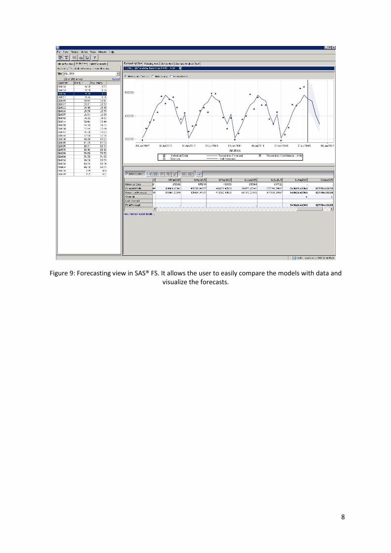
Figure 9: Forecasting view in SAS® FS. It allows the user to easily compare the models with data and visualize the forecasts.

9

6. TIME REQUIREMENTS AND INTERPOLATION

The sales management team operates mainly in weekly cycles. Although analyzing sales on a weekly

basis allows for a greater control, it presents some disadvantages over monthly cycle. The number of

weeks in a given year is not well defined and a specific week does not start in the same day in distinct

years. This can complicate the analysis of sales if the algorithms and software are not prepared to

handle the issue. Furthermore, weekly data is more susceptible to random fluctuations than monthly

data. For these reasons it was decided to use two approaches. The first approach uses weekly data to

train the forecasting models that outputs weekly forecasts. The second approach aggregates the

weekly data into monthly data that is used to train the models. The monthly forecasts are then

interpolated into weekly results to be compared with the competitor. In the next section the second

approach is discussed. Using two approaches allows to diversify and analyze the effects of

granularity.

6.1. MONTHLY TO WEEKLY INTERPOLATION

In this section the interpolation methods used on the monthly forecasts are discussed. In order to

obtain weekly forecasts, as demanded by the client, it is required to divide the monthly sales

forecasts among the weeks that belong to each month, i.e. to perform interpolation of the results.

SAS® has a procedure called PROC EXPAND that allows to change the frequency of the time series

data. The frequency of the data can either be increased or decreased according with the native

frequency and the frequency required for analysis.

The process of gathering records of higher frequency into a lower sampling is called

aggregation. The most common methods to aggregate data is summation or averaging.

These are used depending on the proprieties of the data. Take, for instance, records on oil

daily production and daily atmospheric pressure in an oil field operation. Aggregating this

data on a monthly bases requires to sum the oil production and average (or another

operation) the atmospheric pressure over the days of the month.

The estimation of higher sampling frequency observations from a time series with lower

sampling frequency is called interpolation. This is can be achieved using distinct algorithms

with different degrees of sophistication. 15

PROC EXPAND requires the data to be formatted in a specific way. The usage of the original data

would produce errors due to repeated dates. The data, therefore, was manipulated in SAS®

Enterprise Guide to achieve the required format. The data has now a column for each series and a

time column as can be seen in the Table 4.

10

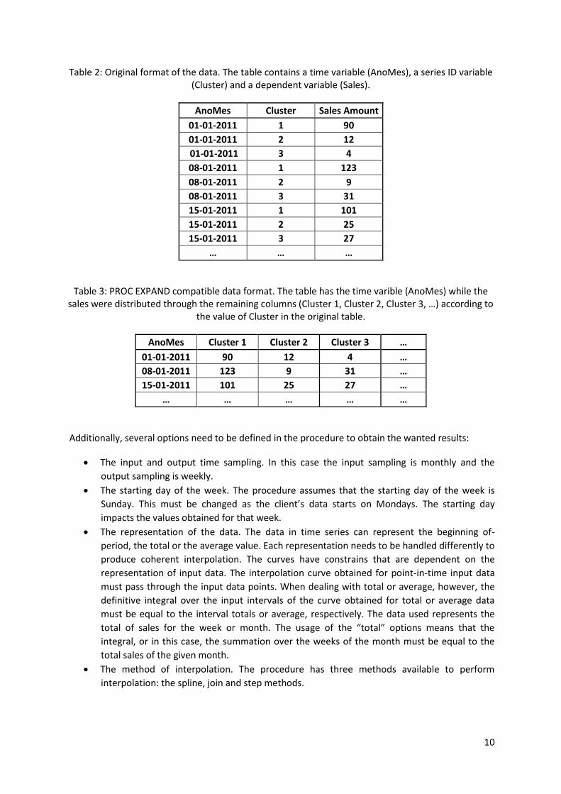
Table 2: Original format of the data. The table contains a time variable (AnoMes), a series ID variable (Cluster) and a dependent variable (Sales).

AnoMes Cluster Sales Amount

01-01-2011 1 90

01-01-2011 2 12

01-01-2011 3 4

08-01-2011 1 123

08-01-2011 2 9

08-01-2011 3 31

15-01-2011 1 101

15-01-2011 2 25

15-01-2011 3 27

… … …

Table 3: PROC EXPAND compatible data format. The table has the time varible (AnoMes) while the sales were distributed through the remaining columns (Cluster 1, Cluster 2, Cluster 3, …) according to

the value of Cluster in the original table.

AnoMes Cluster 1 Cluster 2 Cluster 3 …

01-01-2011 90 12 4 …

08-01-2011 123 9 31 …

15-01-2011 101 25 27 …

… … … … …

Additionally, several options need to be defined in the procedure to obtain the wanted results:

The input and output time sampling. In this case the input sampling is monthly and the

output sampling is weekly.

The starting day of the week. The procedure assumes that the starting day of the week is

Sunday. This must be changed as the client’s data starts on Mondays. The starting day

impacts the values obtained for that week.

The representation of the data. The data in time series can represent the beginning of-

period, the total or the average value. Each representation needs to be handled differently to

produce coherent interpolation. The curves have constrains that are dependent on the

representation of input data. The interpolation curve obtained for point-in-time input data

must pass through the input data points. When dealing with total or average, however, the

definitive integral over the input intervals of the curve obtained for total or average data

must be equal to the interval totals or average, respectively. The data used represents the

total of sales for the week or month. The usage of the “total” options means that the

integral, or in this case, the summation over the weeks of the month must be equal to the

total sales of the given month.

The method of interpolation. The procedure has three methods available to perform

interpolation: the spline, join and step methods.

11

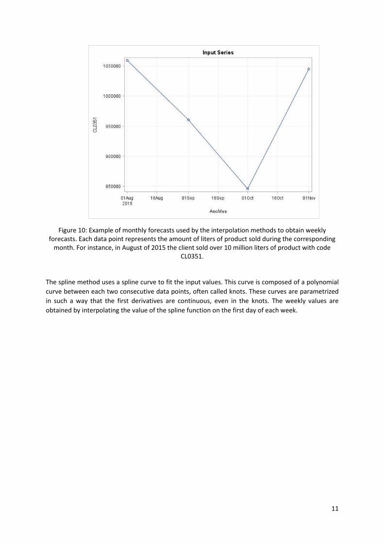
Figure 10: Example of monthly forecasts used by the interpolation methods to obtain weekly forecasts. Each data point represents the amount of liters of product sold during the corresponding

month. For instance, in August of 2015 the client sold over 10 million liters of product with code CL0351.

The spline method uses a spline curve to fit the input values. This curve is composed of a polynomial

curve between each two consecutive data points, often called knots. These curves are parametrized

in such a way that the first derivatives are continuous, even in the knots. The weekly values are

obtained by interpolating the value of the spline function on the first day of each week.

12

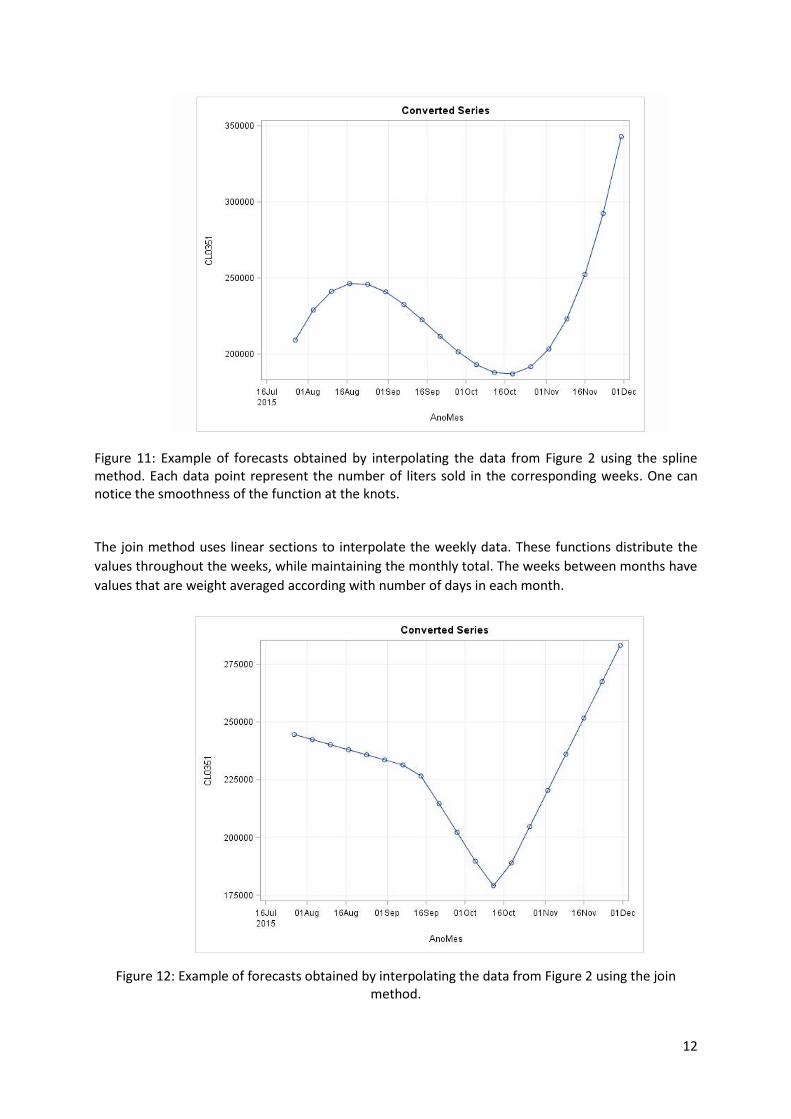
Figure 11: Example of forecasts obtained by interpolating the data from Figure 2 using the spline method. Each data point represent the number of liters sold in the corresponding weeks. One can notice the smoothness of the function at the knots.

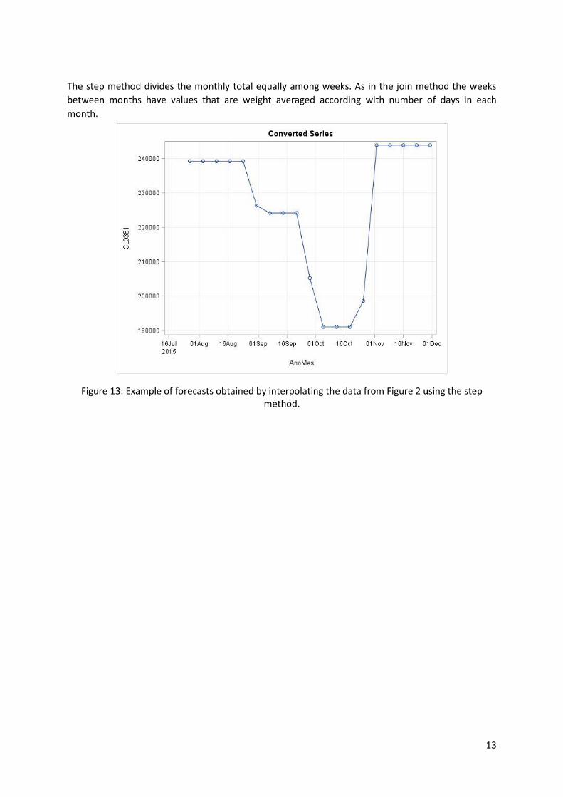
The join method uses linear sections to interpolate the weekly data. These functions distribute the

values throughout the weeks, while maintaining the monthly total. The weeks between months have

values that are weight averaged according with number of days in each month.

Figure 12: Example of forecasts obtained by interpolating the data from Figure 2 using the join method.

13

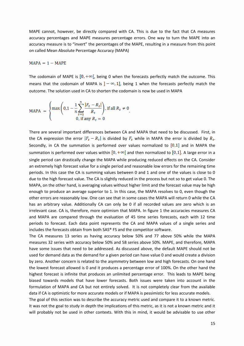
The step method divides the monthly total equally among weeks. As in the join method the weeks

between months have values that are weight averaged according with number of days in each

month.

Figure 13: Example of forecasts obtained by interpolating the data from Figure 2 using the step method.

14

7. RESULTS COMPARISON

The goal of this PoC is to compare the forecasts obtained through the process described above and

the results presented by a competitor. The comparison is achieved by using an accuracy measure

specified by the prospect that is inspired in MAPE:

where is the forecast accuracy for period , is the recorded value for period and is the

forecasted value for period . The previous equation can be rewritten as to simplify the

comprehension

Had not include the max function or the second conditional, the codomain would be . It

is most desirable to have a metric that is restricted within a certain range of values to ease the

interpretation. The max function was introduced to cut-off the codomain at 0 and the second

conditional solves the indetermination issue. The accuracy metric , as now defined, has a

codomain where 1 results when the outcome is equal to the forecast and 0 results when the

or the difference between forecast and outcome is so large that the forecast is considered to

be completely inaccurate.

The accuracy criteria for each time period is then weight averaged to get the overall accuracy of the

forecasts. The weight is defined as the forecasted value for the given time period.

where is the number of periods in which records and forecasts are compared. The evaluation of

the results was designed by the client and thus it has to be used. The accuracy measure used, let it be

called Client Accuracy (CA), is not standard and cannot be easily found in literature. For this reason, it

is appropriate to compare it with known accuracy measures to verify if it can be considered a

reasonable measure. One of the most widely used prediction accuracy measures is MAPE.16 The

default definition of MAPE is

15

MAPE cannot, however, be directly compared with CA. This is due to the fact that CA measures

accuracy percentages and MAPE measures percentage errors. One way to turn the MAPE into an

accuracy measure is to “invert” the percentages of the MAPE, resulting in a measure from this point

on called Mean Absolute Percentage Accuracy (MAPA)

The codomain of MAPE is , being 0 when the forecasts perfectly match the outcome. This

means that the codomain of MAPA is , being 1 when the forecasts perfectly match the

outcome. The solution used in CA to shorten the codomain is now be used in MAPA

There are several important differences between CA and MAPA that need to be discussed. First, in

the CA expression the error is divided by while in MAPA the error is divided by .

Secondly, in CA the summation is performed over values normalized to and in MAPA the

summation is performed over values within and then normalized to . A large error in a

single period can drastically change the MAPA while producing reduced effects on the CA. Consider

an extremely high forecast value for a single period and reasonable low errors for the remaining time

periods. In this case the CA is summing values between 0 and 1 and one of the values is close to 0

due to the high forecast value. The CA is slightly reduced in the process but not so to get value 0. The

MAPA, on the other hand, is averaging values without higher limit and the forecast value may be high

enough to produce an average superior to 1. In this case, the MAPA resolves to 0, even though the

other errors are reasonably low. One can see that in some cases the MAPA will return 0 while the CA

has an arbitrary value. Additionally CA can only be 0 if all recorded values are zero which is an

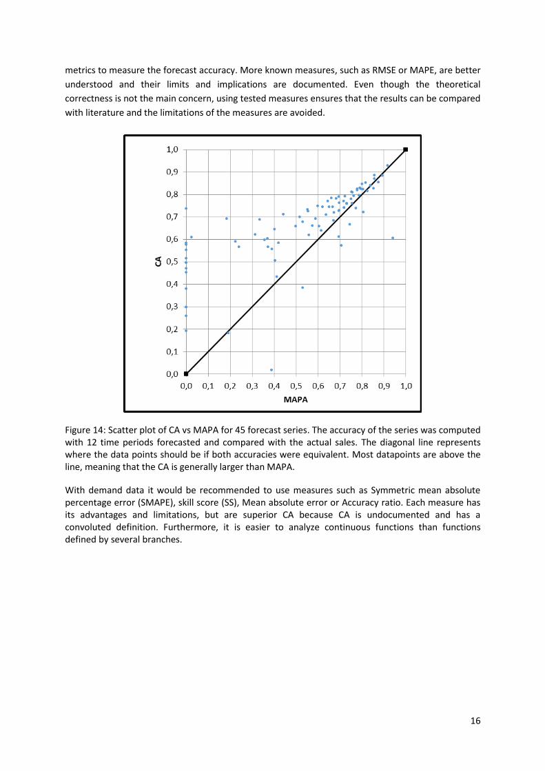
irrelevant case. CA is, therefore, more optimism that MAPA. In figure 1 the accuracies measures CA

and MAPA are compared through the evaluation of 45 time series forecasts, each with 12 time

periods to forecast. Each data point represents the CA and MAPA values of a single series and

includes the forecasts obtain from both SAS® FS and the competitor software.

The CA measures 13 series as having accuracy below 50% and 77 above 50% while the MAPA

measures 32 series with accuracy below 50% and 58 series above 50%. MAPE, and therefore, MAPA

have some issues that need to be addressed. As discussed above, the default MAPE should not be

used for demand data as the demand for a given period can have value 0 and would create a division

by zero. Another concern is related to the asymmetry between low and high forecasts. On one hand

the lowest forecast allowed is 0 and it produces a percentage error of 100%. On the other hand the

highest forecast is infinite that produces an unlimited percentage error. This leads to MAPE being

biased towards models that have lower forecasts. Both issues were taken into account in the

formulation of MAPA and CA but not entirely solved. It is not completely clear from the available

data if CA is optimistic for more accurate models or if MAPA is pessimistic for less accurate models.

The goal of this section was to describe the accuracy metric used and compare it to a known metric.

It was not the goal to study in depth the implications of this metric, as it is not a known metric and it

will probably not be used in other contexts. With this in mind, it would be advisable to use other

16

metrics to measure the forecast accuracy. More known measures, such as RMSE or MAPE, are better

understood and their limits and implications are documented. Even though the theoretical

correctness is not the main concern, using tested measures ensures that the results can be compared

with literature and the limitations of the measures are avoided.

Figure 14: Scatter plot of CA vs MAPA for 45 forecast series. The accuracy of the series was computed with 12 time periods forecasted and compared with the actual sales. The diagonal line represents where the data points should be if both accuracies were equivalent. Most datapoints are above the line, meaning that the CA is generally larger than MAPA.

With demand data it would be recommended to use measures such as Symmetric mean absolute percentage error (SMAPE), skill score (SS), Mean absolute error or Accuracy ratio. Each measure has its advantages and limitations, but are superior CA because CA is undocumented and has a convoluted definition. Furthermore, it is easier to analyze continuous functions than functions defined by several branches.

17

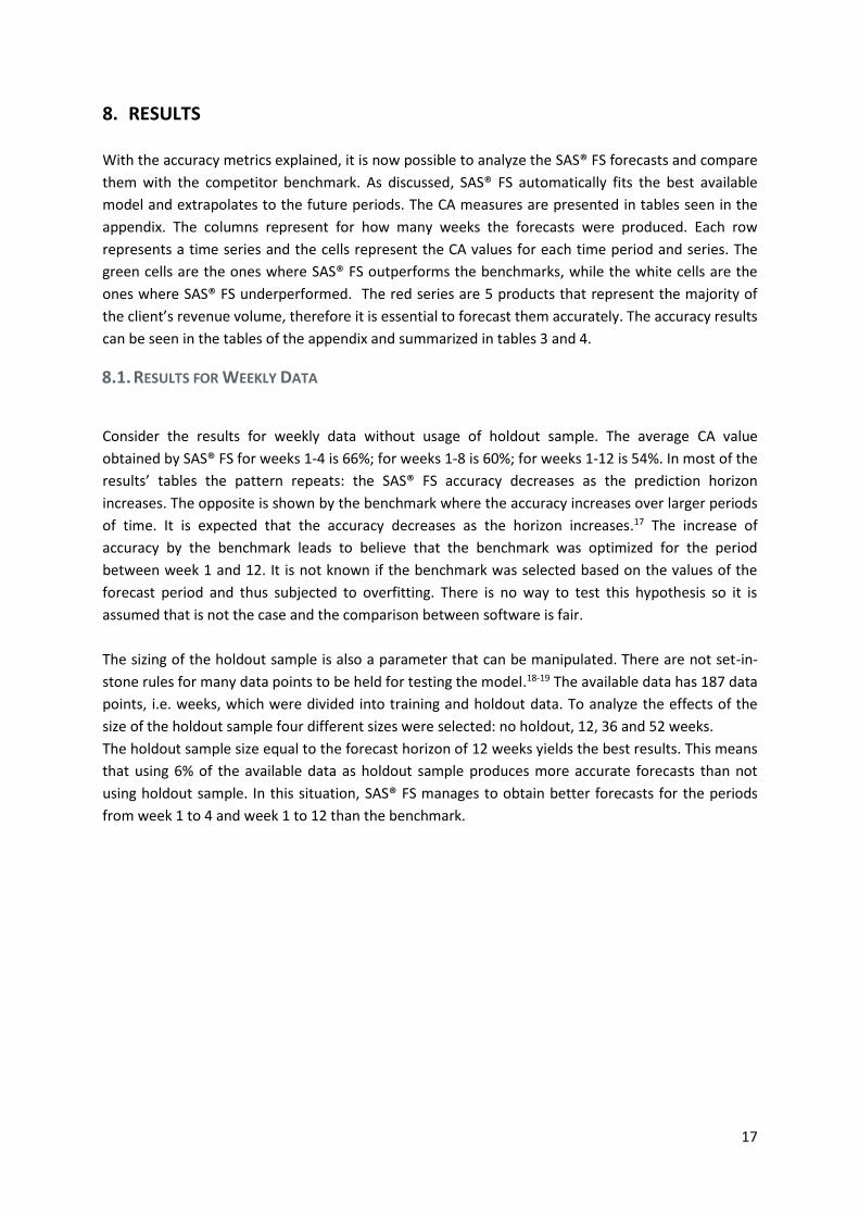
8. RESULTS

With the accuracy metrics explained, it is now possible to analyze the SAS® FS forecasts and compare

them with the competitor benchmark. As discussed, SAS® FS automatically fits the best available

model and extrapolates to the future periods. The CA measures are presented in tables seen in the

appendix. The columns represent for how many weeks the forecasts were produced. Each row

represents a time series and the cells represent the CA values for each time period and series. The

green cells are the ones where SAS® FS outperforms the benchmarks, while the white cells are the

ones where SAS® FS underperformed. The red series are 5 products that represent the majority of

the client’s revenue volume, therefore it is essential to forecast them accurately. The accuracy results

can be seen in the tables of the appendix and summarized in tables 3 and 4.

8.1. RESULTS FOR WEEKLY DATA

Consider the results for weekly data without usage of holdout sample. The average CA value

obtained by SAS® FS for weeks 1-4 is 66%; for weeks 1-8 is 60%; for weeks 1-12 is 54%. In most of the

results’ tables the pattern repeats: the SAS® FS accuracy decreases as the prediction horizon

increases. The opposite is shown by the benchmark where the accuracy increases over larger periods

of time. It is expected that the accuracy decreases as the horizon increases.17 The increase of

accuracy by the benchmark leads to believe that the benchmark was optimized for the period

between week 1 and 12. It is not known if the benchmark was selected based on the values of the

forecast period and thus subjected to overfitting. There is no way to test this hypothesis so it is

assumed that is not the case and the comparison between software is fair.

The sizing of the holdout sample is also a parameter that can be manipulated. There are not set-in-

stone rules for many data points to be held for testing the model.18-19 The available data has 187 data

points, i.e. weeks, which were divided into training and holdout data. To analyze the effects of the

size of the holdout sample four different sizes were selected: no holdout, 12, 36 and 52 weeks.

The holdout sample size equal to the forecast horizon of 12 weeks yields the best results. This means

that using 6% of the available data as holdout sample produces more accurate forecasts than not

using holdout sample. In this situation, SAS® FS manages to obtain better forecasts for the periods

from week 1 to 4 and week 1 to 12 than the benchmark.

18

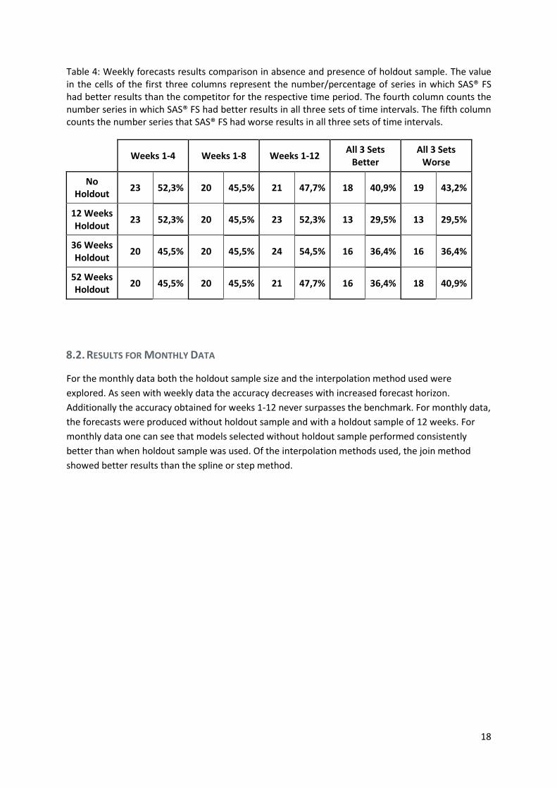
Table 4: Weekly forecasts results comparison in absence and presence of holdout sample. The value in the cells of the first three columns represent the number/percentage of series in which SAS® FS had better results than the competitor for the respective time period. The fourth column counts the number series in which SAS® FS had better results in all three sets of time intervals. The fifth column counts the number series that SAS® FS had worse results in all three sets of time intervals.

Weeks 1-4 Weeks 1-8 Weeks 1-12

All 3 Sets Better

All 3 Sets Worse

No Holdout

23 52,3% 20 45,5% 21 47,7% 18 40,9% 19 43,2%

12 Weeks Holdout

23 52,3% 20 45,5% 23 52,3% 13 29,5% 13 29,5%

36 Weeks Holdout

20 45,5% 20 45,5% 24 54,5% 16 36,4% 16 36,4%

52 Weeks Holdout

20 45,5% 20 45,5% 21 47,7% 16 36,4% 18 40,9%

8.2. RESULTS FOR MONTHLY DATA

For the monthly data both the holdout sample size and the interpolation method used were

explored. As seen with weekly data the accuracy decreases with increased forecast horizon.

Additionally the accuracy obtained for weeks 1-12 never surpasses the benchmark. For monthly data,

the forecasts were produced without holdout sample and with a holdout sample of 12 weeks. For

monthly data one can see that models selected without holdout sample performed consistently

better than when holdout sample was used. Of the interpolation methods used, the join method

showed better results than the spline or step method.

19

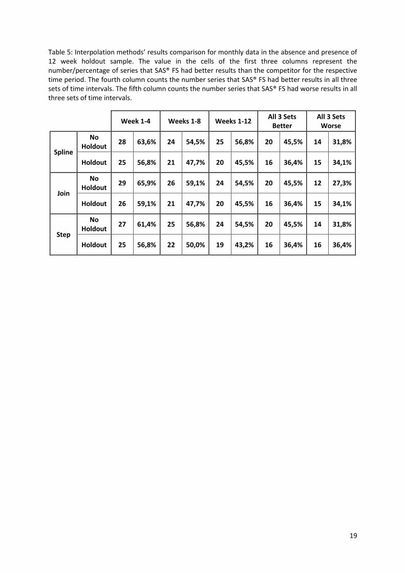
Table 5: Interpolation methods’ results comparison for monthly data in the absence and presence of 12 week holdout sample. The value in the cells of the first three columns represent the number/percentage of series that SAS® FS had better results than the competitor for the respective time period. The fourth column counts the number series that SAS® FS had better results in all three sets of time intervals. The fifth column counts the number series that SAS® FS had worse results in all three sets of time intervals.

Week 1-4 Weeks 1-8 Weeks 1-12

All 3 Sets Better

All 3 Sets Worse

Spline

No Holdout

28 63,6% 24 54,5% 25 56,8% 20 45,5% 14 31,8%

Holdout 25 56,8% 21 47,7% 20 45,5% 16 36,4% 15 34,1%

Join

No Holdout

29 65,9% 26 59,1% 24 54,5% 20 45,5% 12 27,3%

Holdout 26 59,1% 21 47,7% 20 45,5% 16 36,4% 15 34,1%

Step

No Holdout

27 61,4% 25 56,8% 24 54,5% 20 45,5% 14 31,8%

Holdout 25 56,8% 22 50,0% 19 43,2% 16 36,4% 16 36,4%

20

8.3. DISCUSSION OF RESULTS

The SAS® FS is consistently accurate for shorter forecast horizons but the accuracy does not hold for

longer periods. This might be due to several reasons. The small amount of historical data available

might not be enough to train models with large forecast horizons. Although there are no specific

rules or guidelines, if the forecaster wants to increase the forecast horizon he should have increased

historical data to fuel the models. The available data might be enough for a four week forecast

horizon but not for a twelve forecast horizon.

The lower accuracy might also be a consequence of the limited number of variables available, as no

independent variable is used. It is impossible to determine how much the addition of explanatory

variables would improve the accuracy of the models. The demand for beverages is clearly influenced

by the weather conditions at the point-of-sales. Hotter and drier conditions lead to higher

consumption of beverages comparing with colder and rainier conditions. Sales and marketing

campaigns have also a role in clients’ behavior. It is expected that sales increase during sales but

decrease afterwards due to cannibalized demand. Other events such as festivals, concerts or sports

activities increase the consumption of beverages. All these effects are not taken into account which

can compromise the effectiveness of the forecasts. One of the major advantages of SAS® FS is the

ability to use events to explain variations that are caused by known occurrences, which can reduce

the impact of demand spikes on the overall forecasts.

21

9. CONCLUSIONS

The internship provided an excellent coverage of both technical knowledge and on-hands experience

on pre-sales activities. It showcased that more than just modeling knowledge, it is require to

understand the business and how to meet with the prospect’s needs.

SAS® FS is tool capable of providing as accurate results as the competitor even in the absence of

independent variables, event data or external sources of data to complement the models. It is

advisable, however, that such variables are used when developing future forecasting models in order

to take full use of the capabilities of SAS® FS. Additionally, when comparing forecasts the prospect

should have selected a widely known accuracy measure whose advantages and biases are

understood.

22

10. BIBLIOGRAPHY

Illinois Agronomy Handbook. 1st ed. Urbana, Ill.: University of Illinois at Urbana-Champaign, College

of Agricultural, Consumer and Environmental Sciences; 2000.

Wheeler Demarée G. The weather of the Waterloo campaign 16 to 18 June 1815: did it change the

course of history?. Weather. 2005;60(6):159-164. doi:10.1256/wea.246.04.

Ross J., Stagg J. The Forecast For D-Day And The Weatherman Behind Ike's Greatest Gamble. 1st ed.

Beevor A. D-Day. 1st ed. New York: Viking; 2009.

Whitmarsh A. D-Day In Photographs. 1st ed. Stroud: History; 2009.

Butler A, Thurston H, Attwater D. Butler's Lives Of The Saints. 1st ed. New York: P.J. Kenedy & Sons;

1956.

Jenks S. Astrometeorology in the Middle Ages. Isis. 1983;74(2):185-210. doi:10.1086/353243.

Goldstein M. The Complete Idiot's Guide To Weather. 1st ed. New York: Alpha Books; 1999.

Zissis, Dimitrios; Xidias, Elias; Lekkas, Dimitrios (2015). "Real-time vessel behavior prediction".

Evolving Systems. 7: 1–12. doi:10.1007/s12530-015-9133-5

SAS Forecast Server Automates Business Forecasting. Sascom. 2016. Available at:

http://www.sas.com/en_us/software/analytics/forecastserver.html. Accessed October 22, 2016.

Introducing SAS® Forecast Studio. In: SUGI 30.; 2005. Available at:

http://www2.sas.com/proceedings/sugi30/toc.html#st. Accessed October 24, 2016.

SAS Institute Inc. 2015. SAS/ETS® 14.1 User’s Guide. Cary, NC: SAS Institute Inc.

Yokuma JArmstrong J. Beyond accuracy: Comparison of criteria used to select forecasting methods.

International Journal of Forecasting. 1995;11(4):591-597. doi:10.1016/0169-2070(95)00615-x.

Karp A. Time Series Magic: Smoothing, Interpolating, Expanding and Collapsing Time Series Data with

PROC EXPAND. Available at: http://www.lexjansen.com/nesug/nesug97/advtut/karp.pdf. Accessed

November 5, 2016.

Hyndman Rathanasopoulos G. Forecasting: Principles And Practice.; 2013.

Smith Sincich T. An Empirical Analysis of the Effect of Length of Forecast Horizon on Population

Forecast Errors. Demography. 1991;28(2):261. doi:10.2307/2061279

Picard RCook R. Cross-Validation of Regression Models. Journal of the American Statistical

Association. 1984;79(387):575. doi:10.2307/2288403.

Chatfield C. The Analysis Of Time Series. 1st ed. Boca Raton, FL: Chapman & Hall/CRC; 2004.

23

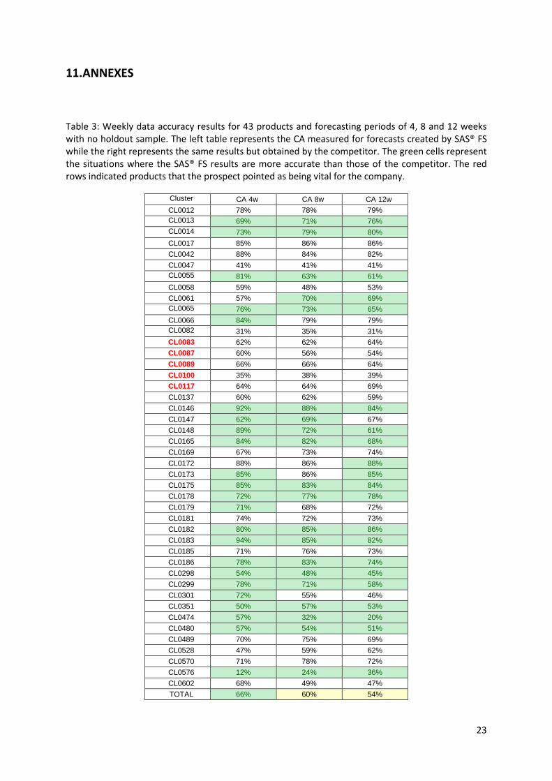
11. ANNEXES

Table 3: Weekly data accuracy results for 43 products and forecasting periods of 4, 8 and 12 weeks with no holdout sample. The left table represents the CA measured for forecasts created by SAS® FS while the right represents the same results but obtained by the competitor. The green cells represent the situations where the SAS® FS results are more accurate than those of the competitor. The red rows indicated products that the prospect pointed as being vital for the company.

Cluster CA 4w CA 8w CA 12w

CL0012 78% 78% 79%

CL0013 69% 71% 76%

CL0014 73% 79% 80%

CL0017 85% 86% 86%

CL0042 88% 84% 82%

CL0047 41% 41% 41%

CL0055 81% 63% 61%

CL0058 59% 48% 53%

CL0061 57% 70% 69%

CL0065 76% 73% 65%

CL0066 84% 79% 79%

CL0082 31% 35% 31%

CL0083 62% 62% 64%

CL0087 60% 56% 54%

CL0089 66% 66% 64%

CL0100 35% 38% 39%

CL0117 64% 64% 69%

CL0137 60% 62% 59%

CL0146 92% 88% 84%

CL0147 62% 69% 67%

CL0148 89% 72% 61%

CL0165 84% 82% 68%

CL0169 67% 73% 74%

CL0172 88% 86% 88%

CL0173 85% 86% 85%

CL0175 85% 83% 84%

CL0178 72% 77% 78%

CL0179 71% 68% 72%

CL0181 74% 72% 73%

CL0182 80% 85% 86%

CL0183 94% 85% 82%

CL0185 71% 76% 73%

CL0186 78% 83% 74%

CL0298 54% 48% 45%

CL0299 78% 71% 58%

CL0301 72% 55% 46%

CL0351 50% 57% 53%

CL0474 57% 32% 20%

CL0480 57% 54% 51%

CL0489 70% 75% 69%

CL0528 47% 59% 62%

CL0570 71% 78% 72%

CL0576 12% 24% 36%

CL0602 68% 49% 47%

TOTAL 66% 60% 54%

24

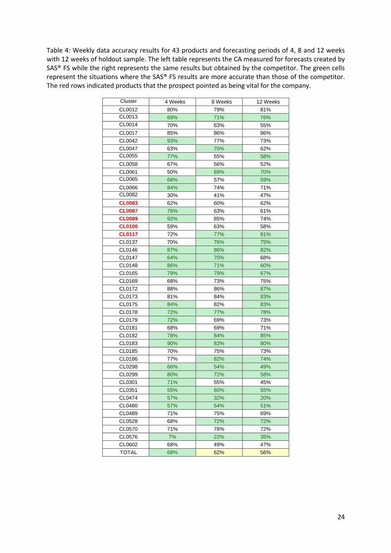
Table 4: Weekly data accuracy results for 43 products and forecasting periods of 4, 8 and 12 weeks with 12 weeks of holdout sample. The left table represents the CA measured for forecasts created by SAS® FS while the right represents the same results but obtained by the competitor. The green cells represent the situations where the SAS® FS results are more accurate than those of the competitor. The red rows indicated products that the prospect pointed as being vital for the company.

Cluster 4 Weeks 8 Weeks 12 Weeks

CL0012 80% 79% 81%

CL0013 69% 71% 76%

CL0014 70% 63% 55%

CL0017 85% 86% 86%

CL0042 93% 77% 73%

CL0047 63% 70% 62%

CL0055 77% 55% 58%

CL0058 67% 56% 52%

CL0061 50% 69% 70%

CL0065 68% 57% 59%

CL0066 84% 74% 71%

CL0082 30% 41% 47%

CL0083 62% 60% 62%

CL0087 76% 63% 61%

CL0089 92% 85% 74%

CL0100 59% 63% 58%

CL0117 72% 77% 81%

CL0137 70% 76% 75%

CL0146 87% 86% 82%

CL0147 64% 70% 68%

CL0148 86% 71% 60%

CL0165 79% 79% 67%

CL0169 68% 73% 75%

CL0172 88% 86% 87%

CL0173 81% 84% 83%

CL0175 84% 82% 83%

CL0178 72% 77% 78%

CL0179 72% 69% 73%

CL0181 68% 69% 71%

CL0182 78% 84% 85%

CL0183 90% 83% 80%

CL0185 70% 75% 73%

CL0186 77% 82% 74%

CL0298 66% 54% 49%

CL0299 80% 72% 58%

CL0301 71% 55% 45%

CL0351 55% 60% 55%

CL0474 57% 32% 20%

CL0480 57% 54% 51%

CL0489 71% 75% 69%

CL0528 68% 72% 72%

CL0570 71% 78% 72%

CL0576 7% 22% 35%

CL0602 68% 49% 47%

TOTAL 68% 62% 56%

25

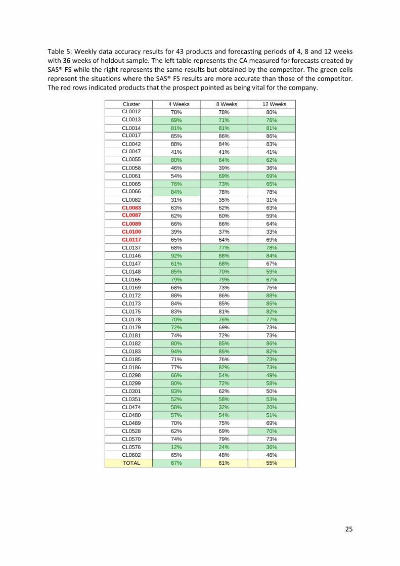
Table 5: Weekly data accuracy results for 43 products and forecasting periods of 4, 8 and 12 weeks with 36 weeks of holdout sample. The left table represents the CA measured for forecasts created by SAS® FS while the right represents the same results but obtained by the competitor. The green cells represent the situations where the SAS® FS results are more accurate than those of the competitor. The red rows indicated products that the prospect pointed as being vital for the company.

Cluster 4 Weeks 8 Weeks 12 Weeks

CL0012 78% 78% 80%

CL0013 69% 71% 76%

CL0014 81% 81% 81%

CL0017 85% 86% 86%

CL0042 88% 84% 83%

CL0047 41% 41% 41%

CL0055 80% 64% 62%

CL0058 46% 39% 36%

CL0061 54% 69% 69%

CL0065 76% 73% 65%

CL0066 84% 78% 78%

CL0082 31% 35% 31%

CL0083 63% 62% 63%

CL0087 62% 60% 59%

CL0089 66% 66% 64%

CL0100 39% 37% 33%

CL0117 65% 64% 69%

CL0137 68% 77% 78%

CL0146 92% 88% 84%

CL0147 61% 68% 67%

CL0148 85% 70% 59%

CL0165 79% 79% 67%

CL0169 68% 73% 75%

CL0172 88% 86% 88%

CL0173 84% 85% 85%

CL0175 83% 81% 82%

CL0178 70% 76% 77%

CL0179 72% 69% 73%

CL0181 74% 72% 73%

CL0182 80% 85% 86%

CL0183 94% 85% 82%

CL0185 71% 76% 73%

CL0186 77% 82% 73%

CL0298 66% 54% 49%

CL0299 80% 72% 58%

CL0301 83% 62% 50%

CL0351 52% 58% 53%

CL0474 58% 32% 20%

CL0480 57% 54% 51%

CL0489 70% 75% 69%

CL0528 62% 69% 70%

CL0570 74% 79% 73%

CL0576 12% 24% 36%

CL0602 65% 48% 46%

TOTAL 67% 61% 55%

26

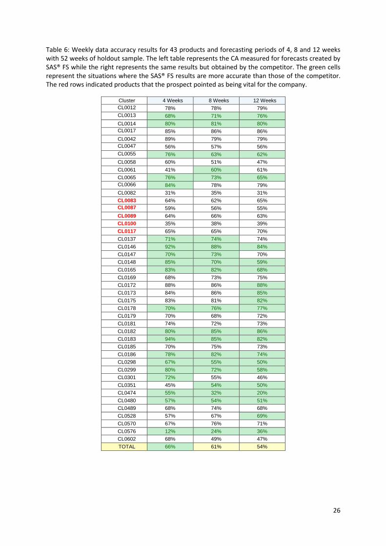
Table 6: Weekly data accuracy results for 43 products and forecasting periods of 4, 8 and 12 weeks with 52 weeks of holdout sample. The left table represents the CA measured for forecasts created by SAS® FS while the right represents the same results but obtained by the competitor. The green cells represent the situations where the SAS® FS results are more accurate than those of the competitor. The red rows indicated products that the prospect pointed as being vital for the company.

Cluster 4 Weeks 8 Weeks 12 Weeks

CL0012 78% 78% 79%

CL0013 68% 71% 76%

CL0014 80% 81% 80%

CL0017 85% 86% 86%

CL0042 89% 79% 79%

CL0047 56% 57% 56%

CL0055 76% 63% 62%

CL0058 60% 51% 47%

CL0061 41% 60% 61%

CL0065 76% 73% 65%

CL0066 84% 78% 79%

CL0082 31% 35% 31%

CL0083 64% 62% 65%

CL0087 59% 56% 55%

CL0089 64% 66% 63%

CL0100 35% 38% 39%

CL0117 65% 65% 70%

CL0137 71% 74% 74%

CL0146 92% 88% 84%

CL0147 70% 73% 70%

CL0148 85% 70% 59%

CL0165 83% 82% 68%

CL0169 68% 73% 75%

CL0172 88% 86% 88%

CL0173 84% 86% 85%

CL0175 83% 81% 82%

CL0178 70% 76% 77%

CL0179 70% 68% 72%

CL0181 74% 72% 73%

CL0182 80% 85% 86%

CL0183 94% 85% 82%

CL0185 70% 75% 73%

CL0186 78% 82% 74%

CL0298 67% 55% 50%

CL0299 80% 72% 58%

CL0301 72% 55% 46%

CL0351 45% 54% 50%

CL0474 55% 32% 20%

CL0480 57% 54% 51%

CL0489 68% 74% 68%

CL0528 57% 67% 69%

CL0570 67% 76% 71%

CL0576 12% 24% 36%

CL0602 68% 49% 47%

TOTAL 66% 61% 54%

27

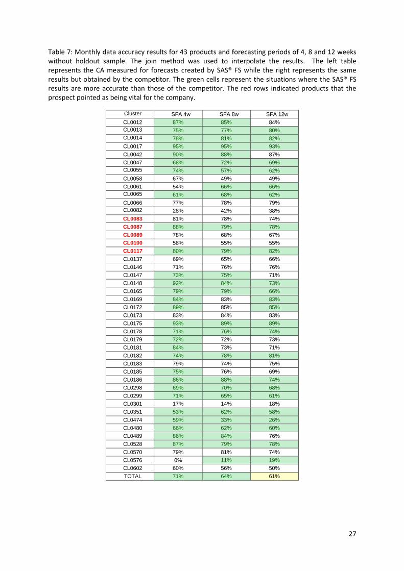
Table 7: Monthly data accuracy results for 43 products and forecasting periods of 4, 8 and 12 weeks without holdout sample. The join method was used to interpolate the results. The left table represents the CA measured for forecasts created by SAS® FS while the right represents the same results but obtained by the competitor. The green cells represent the situations where the SAS® FS results are more accurate than those of the competitor. The red rows indicated products that the prospect pointed as being vital for the company.

Cluster SFA 4w SFA 8w SFA 12w

CL0012 87% 85% 84%

CL0013 75% 77% 80%

CL0014 78% 81% 82%

CL0017 95% 95% 93%

CL0042 90% 88% 87%

CL0047 68% 72% 69%

CL0055 74% 57% 62%

CL0058 67% 49% 49%

CL0061 54% 66% 66%

CL0065 61% 68% 62%

CL0066 77% 78% 79%

CL0082 28% 42% 38%

CL0083 81% 78% 74%

CL0087 88% 79% 78%

CL0089 78% 68% 67%

CL0100 58% 55% 55%

CL0117 80% 79% 82%

CL0137 69% 65% 66%

CL0146 71% 76% 76%

CL0147 73% 75% 71%

CL0148 92% 84% 73%

CL0165 79% 79% 66%

CL0169 84% 83% 83%

CL0172 89% 85% 85%

CL0173 83% 84% 83%

CL0175 93% 89% 89%

CL0178 71% 76% 74%

CL0179 72% 72% 73%

CL0181 84% 73% 71%

CL0182 74% 78% 81%

CL0183 79% 74% 75%

CL0185 75% 76% 69%

CL0186 86% 88% 74%

CL0298 69% 70% 68%

CL0299 71% 65% 61%

CL0301 17% 14% 18%

CL0351 53% 62% 58%

CL0474 59% 33% 26%

CL0480 66% 62% 60%

CL0489 86% 84% 76%

CL0528 87% 79% 78%

CL0570 79% 81% 74%

CL0576 0% 11% 19%

CL0602 60% 56% 50%

TOTAL 71% 64% 61%

28

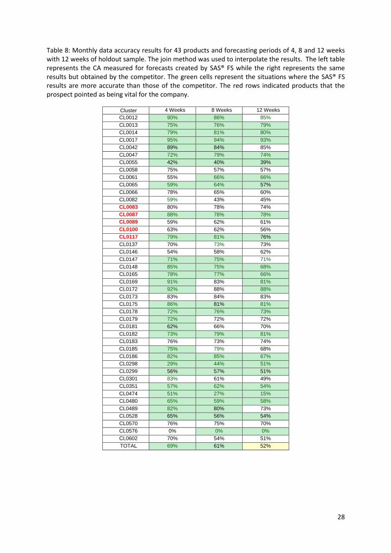
Table 8: Monthly data accuracy results for 43 products and forecasting periods of 4, 8 and 12 weeks with 12 weeks of holdout sample. The join method was used to interpolate the results. The left table represents the CA measured for forecasts created by SAS® FS while the right represents the same results but obtained by the competitor. The green cells represent the situations where the SAS® FS results are more accurate than those of the competitor. The red rows indicated products that the prospect pointed as being vital for the company.

Cluster 4 Weeks 8 Weeks 12 Weeks

CL0012 90% 86% 85%

CL0013 75% 76% 79%

CL0014 79% 81% 80%

CL0017 95% 94% 93%

CL0042 89% 84% 85%

CL0047 72% 79% 74%

CL0055 42% 40% 39%

CL0058 75% 57% 57%

CL0061 55% 66% 66%

CL0065 59% 64% 57%

CL0066 78% 65% 60%

CL0082 59% 43% 45%

CL0083 80% 78% 74%

CL0087 88% 78% 78%

CL0089 59% 62% 61%

CL0100 63% 62% 56%

CL0117 79% 81% 76%

CL0137 70% 73% 73%

CL0146 54% 58% 62%

CL0147 71% 75% 71%

CL0148 85% 75% 68%

CL0165 78% 77% 66%

CL0169 91% 83% 81%

CL0172 92% 88% 88%

CL0173 83% 84% 83%

CL0175 86% 81% 81%

CL0178 72% 76% 73%

CL0179 72% 72% 72%

CL0181 62% 66% 70%

CL0182 73% 79% 81%

CL0183 76% 73% 74%

CL0185 75% 79% 68%

CL0186 82% 85% 67%

CL0298 29% 44% 51%

CL0299 56% 57% 51%

CL0301 83% 61% 49%

CL0351 57% 62% 54%

CL0474 51% 27% 15%

CL0480 65% 59% 58%

CL0489 82% 80% 73%

CL0528 65% 56% 54%

CL0570 76% 75% 70%

CL0576 0% 0% 0%

CL0602 70% 54% 51%

TOTAL 69% 61% 52%

29

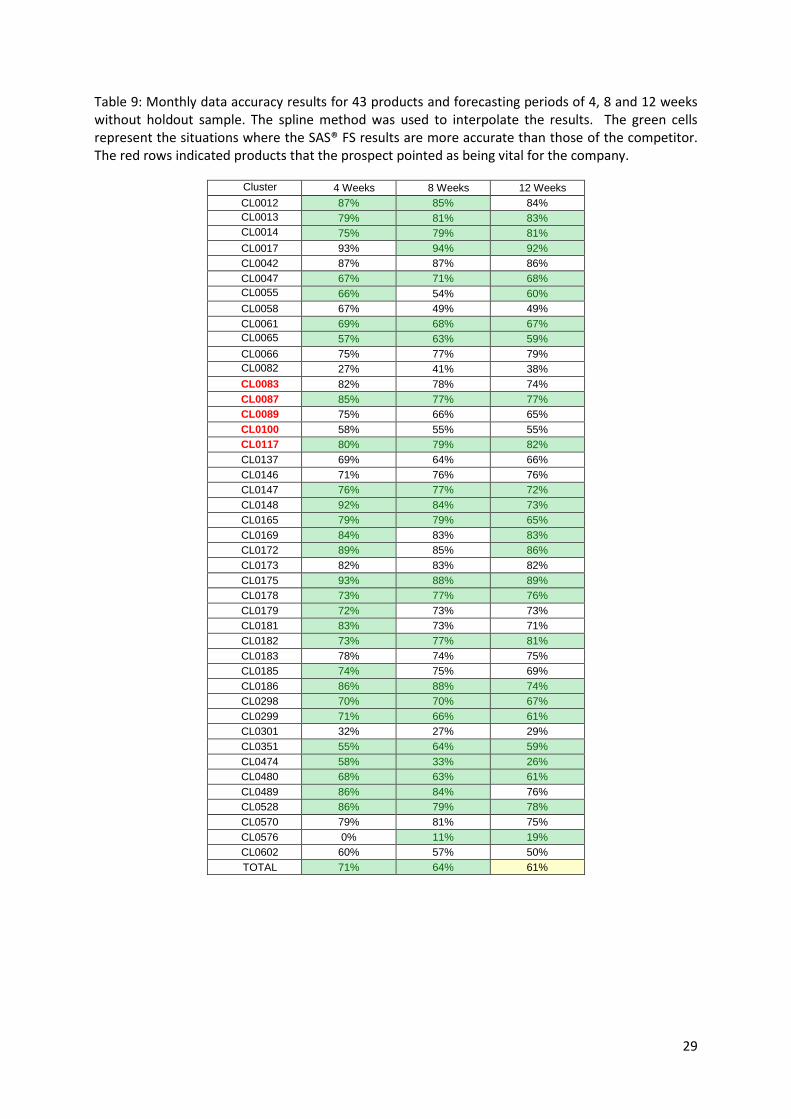
Table 9: Monthly data accuracy results for 43 products and forecasting periods of 4, 8 and 12 weeks without holdout sample. The spline method was used to interpolate the results. The green cells represent the situations where the SAS® FS results are more accurate than those of the competitor. The red rows indicated products that the prospect pointed as being vital for the company.

Cluster 4 Weeks 8 Weeks 12 Weeks

CL0012 87% 85% 84%

CL0013 79% 81% 83%

CL0014 75% 79% 81%

CL0017 93% 94% 92%

CL0042 87% 87% 86%

CL0047 67% 71% 68%

CL0055 66% 54% 60%

CL0058 67% 49% 49%

CL0061 69% 68% 67%

CL0065 57% 63% 59%

CL0066 75% 77% 79%

CL0082 27% 41% 38%

CL0083 82% 78% 74%

CL0087 85% 77% 77%

CL0089 75% 66% 65%

CL0100 58% 55% 55%

CL0117 80% 79% 82%

CL0137 69% 64% 66%

CL0146 71% 76% 76%

CL0147 76% 77% 72%

CL0148 92% 84% 73%

CL0165 79% 79% 65%

CL0169 84% 83% 83%

CL0172 89% 85% 86%

CL0173 82% 83% 82%

CL0175 93% 88% 89%

CL0178 73% 77% 76%

CL0179 72% 73% 73%

CL0181 83% 73% 71%

CL0182 73% 77% 81%

CL0183 78% 74% 75%

CL0185 74% 75% 69%

CL0186 86% 88% 74%

CL0298 70% 70% 67%

CL0299 71% 66% 61%

CL0301 32% 27% 29%

CL0351 55% 64% 59%

CL0474 58% 33% 26%

CL0480 68% 63% 61%

CL0489 86% 84% 76%

CL0528 86% 79% 78%

CL0570 79% 81% 75%

CL0576 0% 11% 19%

CL0602 60% 57% 50%

TOTAL 71% 64% 61%

30

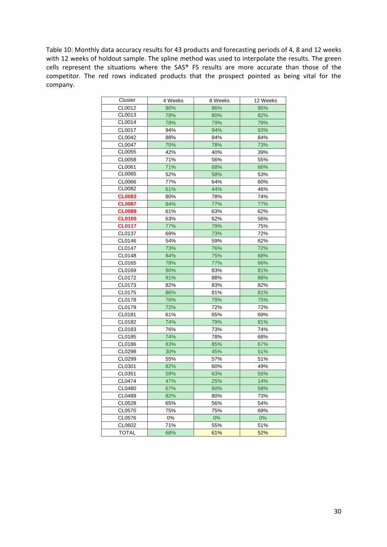
Table 10: Monthly data accuracy results for 43 products and forecasting periods of 4, 8 and 12 weeks with 12 weeks of holdout sample. The spline method was used to interpolate the results. The green cells represent the situations where the SAS® FS results are more accurate than those of the competitor. The red rows indicated products that the prospect pointed as being vital for the company.

Cluster 4 Weeks 8 Weeks 12 Weeks

CL0012 90% 86% 85%

CL0013 78% 80% 82%

CL0014 78% 79% 79%

CL0017 94% 94% 93%

CL0042 88% 84% 84%

CL0047 70% 78% 73%

CL0055 42% 40% 39%

CL0058 71% 56% 55%

CL0061 71% 68% 66%

CL0065 52% 58% 53%

CL0066 77% 64% 60%

CL0082 61% 44% 46%

CL0083 80% 78% 74%

CL0087 84% 77% 77%

CL0089 61% 63% 62%

CL0100 63% 62% 56%

CL0117 77% 79% 75%

CL0137 69% 73% 72%

CL0146 54% 59% 62%

CL0147 73% 76% 72%

CL0148 84% 75% 68%

CL0165 78% 77% 66%

CL0169 90% 83% 81%

CL0172 91% 88% 88%

CL0173 82% 83% 82%

CL0175 86% 81% 81%

CL0178 76% 79% 75%

CL0179 72% 72% 72%

CL0181 61% 65% 69%

CL0182 74% 79% 81%

CL0183 76% 73% 74%

CL0185 74% 78% 68%

CL0186 83% 85% 67%

CL0298 30% 45% 51%

CL0299 55% 57% 51%

CL0301 82% 60% 49%

CL0351 59% 63% 55%

CL0474 47% 25% 14%

CL0480 67% 60% 58%

CL0489 82% 80% 73%

CL0528 65% 56% 54%

CL0570 75% 75% 69%

CL0576 0% 0% 0%

CL0602 71% 55% 51%

TOTAL 68% 61% 52%

31

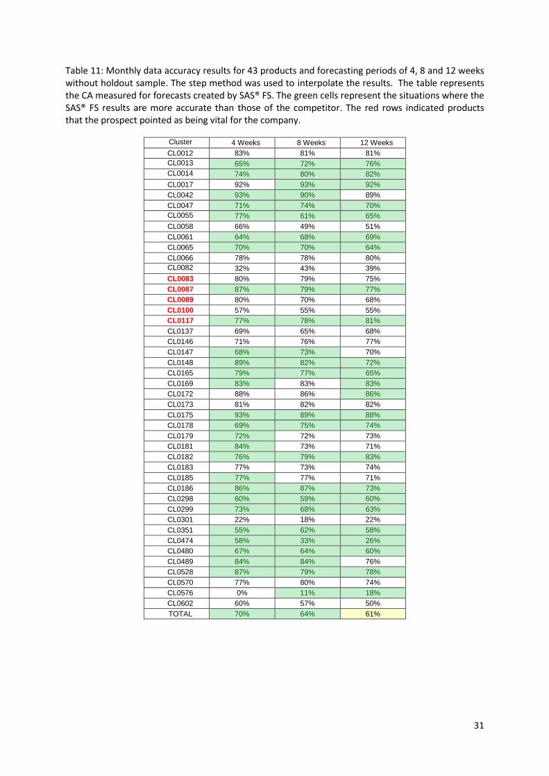
Table 11: Monthly data accuracy results for 43 products and forecasting periods of 4, 8 and 12 weeks without holdout sample. The step method was used to interpolate the results. The table represents the CA measured for forecasts created by SAS® FS. The green cells represent the situations where the SAS® FS results are more accurate than those of the competitor. The red rows indicated products that the prospect pointed as being vital for the company.

Cluster 4 Weeks 8 Weeks 12 Weeks

CL0012 83% 81% 81%

CL0013 65% 72% 76%

CL0014 74% 80% 82%

CL0017 92% 93% 92%

CL0042 93% 90% 89%

CL0047 71% 74% 70%

CL0055 77% 61% 65%

CL0058 66% 49% 51%

CL0061 64% 68% 69%

CL0065 70% 70% 64%

CL0066 78% 78% 80%

CL0082 32% 43% 39%

CL0083 80% 79% 75%

CL0087 87% 79% 77%

CL0089 80% 70% 68%

CL0100 57% 55% 55%

CL0117 77% 78% 81%

CL0137 69% 65% 68%

CL0146 71% 76% 77%

CL0147 68% 73% 70%

CL0148 89% 82% 72%

CL0165 79% 77% 65%

CL0169 83% 83% 83%

CL0172 88% 86% 86%

CL0173 81% 82% 82%

CL0175 93% 89% 88%

CL0178 69% 75% 74%

CL0179 72% 72% 73%

CL0181 84% 73% 71%

CL0182 76% 79% 83%

CL0183 77% 73% 74%

CL0185 77% 77% 71%

CL0186 86% 87% 73%

CL0298 60% 59% 60%

CL0299 73% 68% 63%

CL0301 22% 18% 22%

CL0351 55% 62% 58%

CL0474 58% 33% 26%

CL0480 67% 64% 60%

CL0489 84% 84% 76%

CL0528 87% 79% 78%

CL0570 77% 80% 74%

CL0576 0% 11% 18%

CL0602 60% 57% 50%

TOTAL 70% 64% 61%

32

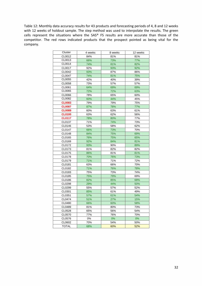
Table 12: Monthly data accuracy results for 43 products and forecasting periods of 4, 8 and 12 weeks with 12 weeks of holdout sample. The step method was used to interpolate the results. The green cells represent the situations where the SAS® FS results are more accurate than those of the competitor. The red rows indicated products that the prospect pointed as being vital for the company.

Cluster 4 weeks 8 weeks 12 weeks

CL0012 84% 81% 81%

CL0013 66% 73% 77%

CL0014 74% 81% 82%

CL0017 92% 93% 92%

CL0042 93% 87% 86%

CL0047 74% 81% 75%

CL0055 42% 40% 39%

CL0058 73% 57% 57%

CL0061 64% 69% 69%

CL0065 72% 72% 63%

CL0066 78% 65% 60%

CL0082 60% 44% 45%

CL0083 79% 79% 75%

CL0087 87% 78% 77%

CL0089 60% 63% 61%

CL0100 63% 62% 56%

CL0117 78% 80% 77%

CL0137 71% 74% 73%

CL0146 53% 58% 62%

CL0147 66% 73% 70%

CL0148 84% 75% 69%

CL0165 76% 75% 65%

CL0169 92% 84% 81%

CL0172 93% 90% 89%

CL0173 81% 82% 82%

CL0175 86% 81% 81%

CL0178 70% 76% 73%

CL0179 71% 71% 72%

CL0181 63% 66% 70%

CL0182 71% 76% 78%

CL0183 75% 73% 74%

CL0185 75% 79% 69%

CL0186 82% 85% 68%

CL0298 29% 44% 50%

CL0299 55% 57% 52%

CL0301 85% 61% 49%

CL0351 57% 61% 54%

CL0474 51% 27% 15%

CL0480 66% 60% 58%

CL0489 81% 80% 73%

CL0528 65% 56% 54%

CL0570 77% 76% 70%

CL0576 0% 0% 0%

CL0602 70% 54% 50%

TOTAL 68% 60% 52%