Embed Size (px)
Citation preview
LAB SESSION INTRODUCTION LIS Summer Workshop 2009
Lab Session Exercises Summer Workshop 2010
SAS version
Luxembourg Income Study
June 27th – July 3rd 2010

CONTENTS
1. INTRODUCTION
Ex. 1: Accessing the LIS Database: the Job Submission Interface (JSI)
2. BASICS I
Ex. 2: Running Descriptive Statistics: Sample and Population Values
3. BASICS II
Ex. 3: Using Subroutines and Loops to Simplify Submissions Involving Several Datasets
Ex. 4: Combining Datasets
4. DEMOGRAPHICS AND EDUCATION
Ex. 5: Children (Household Level)
Ex. 6: Gender (Person Level)
Ex. 7: Comparing educ and peduc
Ex. 8: Comparing Educational Outcomes
5. INCOME DISTRIBUTION I
Ex. 9: Equivalence Scales
Ex. 10: Poverty Lines and Poverty Rates
Ex. 11: Elderly and Child Poverty Rates
6. INCOME DISTRIBUTION II
Ex. 12: Dealing with Extreme Values: Trimming and Bottom- / Top- coding
Ex. 13: Inequality: the Gini Index
Ex. 14: Sensitivity Analysis Using Different Concepts of Income
Ex. 15: Sensitivity Analysis Using Different Equivalence Scales
7. LABOUR MARKET
Ex. 16: Calculating Employment Rates
Ex. 17: Calculating Unemployment Rates
Ex. 18: Person- and Job-specific Characteristics of Employment
8. STACKED DATA
Ex. 19: A Cross-national Comparison Using Stacked Data
9. LWS BASICS
Ex. 20: Differences in Concepts of Net Worth
Ex. 21: Asset Participation
INTRODUCTION
Ex. 1: Accessing the LIS Database: the Job Submission Interface (JSI)


LAB SESSION INTRODUCTION LIS Summer Workshop 2010
1. Accessing the LIS Database: the Job Submission Interface (JSI)
Goal
The Job Submission Interface (JSI) is a secure Java application that allows researchers to:
- write, submit and view job requests (and corresponding outputs); - track the status of the job requests in process ('received', 'processing', 'set for review',
‘refused’, etc.); and - access the history of all job requests ever sent.
The first exercise is an introduction to the JSI to ensure the ability to launch and use it successfully.
Activity
Launch the Job Submission Interface (JSI) application and logon to it with your LIS account.
Submit a simple program to display the following text in your output (or listing): “Your program has run successfully”.
Track the status of your job.
View the resulting listing.
Go to the Job Library window and discard the job; use the advanced search tool to get it back.
Guidelines
Once connected to the Job submission Interface, there are three main tasks that may be carried out:
� Submit jobs through the Job Session window.
- Select a project (LIS, LWS or LES). - Select a statistical package (SAS, SPSS or Stata). - When submitting a job (Job Session window), always add a subject line. - Write your code. - Click on the submit button. - Note that for security reasons, the output of all job requests will be returned to the email
registered in LISSY even if the submission is processed through the JSI. That way, each LIS user will be informed if someone is using his/her userid and password.
� Work with Today's Jobs (Today Jobs window.)
- Watch the status of jobs currently sent to LISSY in the 'jobs in process' panel (top-left). - View the jobs returned by LISSY. - Click on a job in the 'jobs returned' panel (bottom-left). - Click on the 'view job' button. - Click on the 'job text' or 'listing' tabs, respectively, of the right panel to see the request and
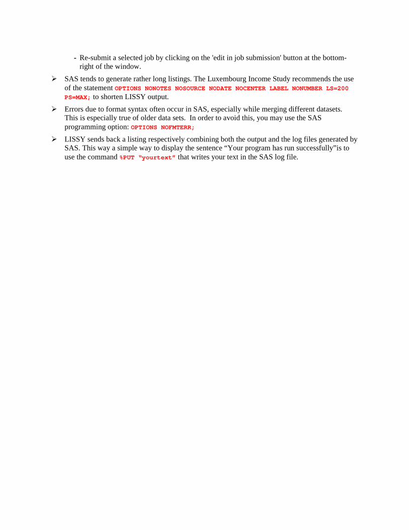
its output. - Re-submit a selected job by clicking on the 'edit in job submission' button at the bottom-
right of the window. � Manage (view, clean and search) all job requests ever sent in the Job Library window.
- View jobs sent over a specific time period. - Clean the library by discarding useless job requests ('discard' button). - Search jobs by keywords.
- Re-submit a selected job by clicking on the 'edit in job submission' button at the bottom-right of the window.
� SAS tends to generate rather long listings. The Luxembourg Income Study recommends the use of the statement OPTIONS NONOTES NOSOURCE NODATE NOCENTER LABEL NONUMBER LS=200
PS=MAX; to shorten LISSY output.
� Errors due to format syntax often occur in SAS, especially while merging different datasets. This is especially true of older data sets. In order to avoid this, you may use the SAS programming option: OPTIONS NOFMTERR;
� LISSY sends back a listing respectively combining both the output and the log files generated by SAS. This way a simple way to display the sentence “Your program has run successfully”is to use the command %PUT “yourtext” that writes your text in the SAS log file.

LAB SESSION INTRODUCTION LIS Summer Workshop 2010
Program
OPTIONS NONOTES NOSOURCE;
%PUT "Congratulations! Your message was received.";
Comments
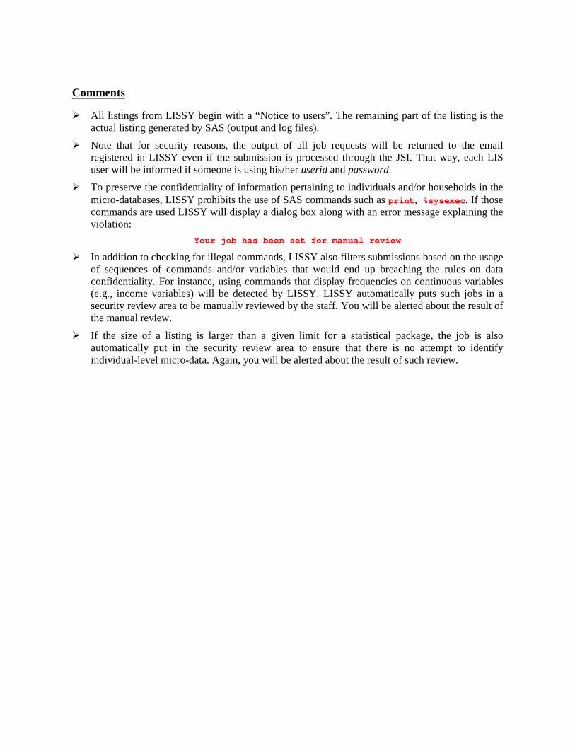
� All listings from LISSY begin with a “Notice to users”. The remaining part of the listing is the actual listing generated by SAS (output and log files).
� Note that for security reasons, the output of all job requests will be returned to the email registered in LISSY even if the submission is processed through the JSI. That way, each LIS user will be informed if someone is using his/her userid and password.
� To preserve the confidentiality of information pertaining to individuals and/or households in the micro-databases, LISSY prohibits the use of SAS commands such as print , %sysexec . If those commands are used LISSY will display a dialog box along with an error message explaining the violation:
Your job has been set for manual review
� In addition to checking for illegal commands, LISSY also filters submissions based on the usage of sequences of commands and/or variables that would end up breaching the rules on data confidentiality. For instance, using commands that display frequencies on continuous variables (e.g., income variables) will be detected by LISSY. LISSY automatically puts such jobs in a security review area to be manually reviewed by the staff. You will be alerted about the result of the manual review.
� If the size of a listing is larger than a given limit for a statistical package, the job is also automatically put in the security review area to ensure that there is no attempt to identify individual-level micro-data. Again, you will be alerted about the result of such review.
BASICS I
Ex. 2: Running Descriptive Statistics: Sample and Population Values

LAB SESSION BASICS I LIS Summer Workshop 2010
2. Running Descriptive Statistics: Sample and Population Values
Goal
This exercise is an introduction to a few of the variables in the household- and person-level LIS data sets. The exercise concentrates on job syntax, basic descriptive statistics and the use of the weight.
Comparative researchers are typically interested in the characteristics of national populations, not the samples provided. It is very important to understand and use sample weights correctly in order to get representative results for the total underlying population. This exercise shows the differences in statistics between the unweighted sample and the weighted population.
Activity
For Luxembourg 2004 (LU04), create a household-level dataset containing: the household identifier (casenum), household weight (hweight), number of earners in the household (d6), number of children under 18 (d27), whether the head of the household is living in a couple (married), age of the household head (d1), gender of household head (d3), gender of the spouse of the household head (sexsp), and the household net disposable income (dpi).
Find the unweighted and weighted number of observations, mean, median, minimum, and maximum for the continuous variables (including casenum and hweight) and the unweighted and weighted frequencies of the categorical variables.
For the same country, use the person-level data to create a dataset containing: the household identifier (casenum); the person identifier (ppnum); person weight (pweight); age (page); gender (psex); marital status (pmart); relationship to the head of the household (prel); gross wages and salaries (pgwage); and gross wages per unit of time (pgwtime).
Find the unweighted and weighted number of observations, mean, median, minimum, and maximum for the continuous variables (including casenum, ppnum, pweight and page) and the unweighted and weighted frequencies of the categorical variables.
Use the information from your output to answer the following questions:
1. Why can sexsp have a value of -1, but d3 can never be -1?
_____________________________________________________________________________
_____________________________________________________________________________
_____________________________________________________________________________
2. Why do the values of pgwage and pgwtime differ (check the Variables Definition List and the Lissification Table for LU04 on line)?
_____________________________________________________________________________
_____________________________________________________________________________
_____________________________________________________________________________
_____________________________________________________________________________
Guidelines
� When you open a LIS dataset, use the correct alias for the country/year you wish to use. For example:
SET &lu04p;
For more information about the syntax of country/year macros, see the job submission instructions on the LIS web site (Micro-Databases Access � Job Submission Instructions). For a list of available data sets and their 2-digit country codes, go to:
Luxembourg Income Study (LIS) � List of Datasets.
� Only keep the variables you will be using:
(KEEP= casenum d6 d27 married d1 d3 dpi);
This avoids unnecessary burden on the machine so that submitted jobs will run faster.
If you need help determining which variables are categorical, go to the LIS web site and click on Luxembourg Income Study (LIS) � Luxembourg � 2004 (column: Lissification Tables; row: Wave VI). The “Value Labels” column of the Lissification Table delineates the values of categorical variables.
� For this dataset, the weight inflates to the total population in Luxembourg in 2004. This means you can find the population size by looking at the “Sum of Weight.”. Information about sample size and weighted population estimates can be found at Luxembourg Income Study (LIS) � <country> � Weighting Procedures.
� SAS reminder: to run descriptive statistics, use these procedures:
PROC MEANS DATA=dataset <statistics>; VAR variablelist ; WEIGHT yourweight ; RUN;
PROC FREQ DATA=dataset ; TABLES variablelist / < OPTION> WEIGHT yourweight ; RUN;
- By default, SAS generates cumulative frequencies. Add the NOCUM option to the “tables” statement. It suppresses display of cumulative frequencies and cumulative percentages in one-way frequency tables and in list format. Add also the MISSPRINT option to the “tables” statement in order to display missing value frequencies.
� SAS reminder
Descriptive and frequencies can be run by classification variable(s) adding the statement BY
variable . Prior to use it, the dataset must be sorted. To sort the dataset, apply the following procedure:
PROC SORT DATA=dataset ; BY variable ; RUN;
� IMPORTANT: Wait to get your results before sending a new job!
LAB SESSION BASICS I LIS Summer Workshop 2010
Program
OPTIONS NOSOURCE NONOTES NOFMTERR NODATE NOCENTER LABEL NONUMBER LS=200 PS=MAX; DATA lu4h; SET &lu04h (KEEP=casenum d1 hweight dpi d6 married d27 d3 sexsp); RUN; TITLE "LU04H – Run unweighted descriptives – Contin uous household variables"; PROC MEANS DATA=lu4h N MEAN MIN MAX MEDIAN; VAR casenum d1 hweight dpi; RUN; TITLE "LU04H – Run weighted descriptives – Continuo us household variables"; PROC MEANS DATA=lu4h N MEAN MIN MAX MEDIAN SUMWGT; VAR casenum d1 hweight dpi; WEIGHT hweight ; RUN; TITLE "LU04H – Run unweighted descriptives – Catego rical household variables"; PROC FREQ DATA=lu4h; TABLES d6 married d27 d3 sexsp / MISSPRINT NOCUM; RUN; TITLE "LU04H – Run weighted descriptives – Categori cal household variables"; PROC FREQ DATA=lu4h; TABLES d6 married d27 d3 sexsp / MISSPRINT NOCUM; WEIGHT hweight ; RUN; DATA lu4p; SET &lu04p (KEEP=casenum ppnum pweight page pgwage pgwtime psex pmart prel); RUN; TITLE "LU04P – Run unweighted descriptives – Contin uous person-level variables"; PROC MEANS DATA=lu4p N MEAN MIN MAX MEDIAN SUMWGT; VAR casenum ppnum pweight page pgwage pgwtime; RUN; TITLE "LU04P – Run weighted descriptives – Continuo us person-level variables"; PROC MEANS DATA=lu4p N MEAN MIN MAX MEDIAN; VAR casenum ppnum pweight page pgwage pgwtime; WEIGHT pweight; RUN; TITLE "LU04P – Run unweighted descriptives – Catego rical person-level variables"; PROC FREQ DATA=lu4p; TABLES psex pmart prel / MISSPRINT NOCUM; RUN; TITLE "LU04P – Run weighted descriptives – Categori cal person-level variables"; PROC FREQ DATA=lu4p; TABLES psex pmart prel / MISSPRINT NOCUM; WEIGHT pweight; RUN; TITLE;
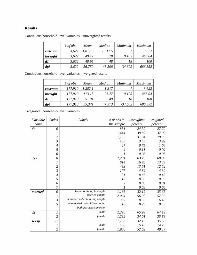
Results
Continuous household-level variables – unweighted results
Continuous household-level variables – weighted results
Categorical household-level variables
# of obs Mean Median Minimum Maximum
casenum 3,622 1,811.5 1,811.5 1 3,622
hweight 3,622 49.12 28 0.105 466.04
d1 3,622 48.95 48 18 100
dpi 3,622 56,750 48,598 -34,602 686,352
# of obs Mean Median Minimum Maximum
casenum 177,910 1,282.1 1,317 1 3,622
hweight 177,910 113.15 96.77 0.105 466.04
d1 177,910 51.04 49 18 100
dpi 177,910 55,371 47,373 -34,602 686,352
Variable name
Codes Labels # of obs in the sample
unweighted percent
weighted percent
d6 0 1 2 3 4 5 6
881 1,444 1,135
130 27 4 1
24.32 39.87 31.34 3.59 0.75 0.11 0.03
27.70 37.92 29.35 3.92 1.04 0.02 0.05
d27 0 1 2 3 4 5 6 7
2,291 614 493 177 31 13 2 1
63.25 16.95 13.61 4.89 0.86 0.36 0.06 0.03
68.96 13.39 12.52 4.30 0.42 0.35 0.01 0.05
married 0 1 3 5
head not living in couple married couple
non-married cohabiting couple
non-married cohabiting couple,
both partners same sex
1,166 2,064
382 10
32.19 56.99 10.55 0.28
35.68 57.35 6.48 0.49
d3 1 2
male
female 2,390 1,232
65.99 34.01
64.12 35.88
sexsp -1 1 2
male
female
1,166 550
1,906
32.19 15.18 52.62
35.68 14.75 49.57
LAB SESSION BASICS I LIS Summer Workshop 2010
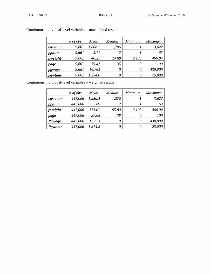
Continuous individual-level variables – unweighted results
Continuous individual-level variables – weighted results
# of obs Mean Median Minimum Maximum
casenum 9,661 1,808.2 1,796 1 3,622
ppnum 9,661 3.11 2 1 63
pweight 9,661 46.27 24.08 0.105 466.04
page 9,661 35.47 35 0 100
pgwage 9,661 16,763 0 0 430,000
pgwtime 9,661 1,234.6 0 0 25,000
# of obs Mean Median Minimum Maximum
casenum 447,006 1,250.4 1,276 1 3,622
ppnum 447,006 2.89 2 1 63
pweight 447,006 113.01 95.80 0.105 466.04
page 447,006 37.65 38 0 100
Pgwage 447,006 17,723 0 0 430,000
Pgwtime 447,006 1,314.2 0 0 25,000
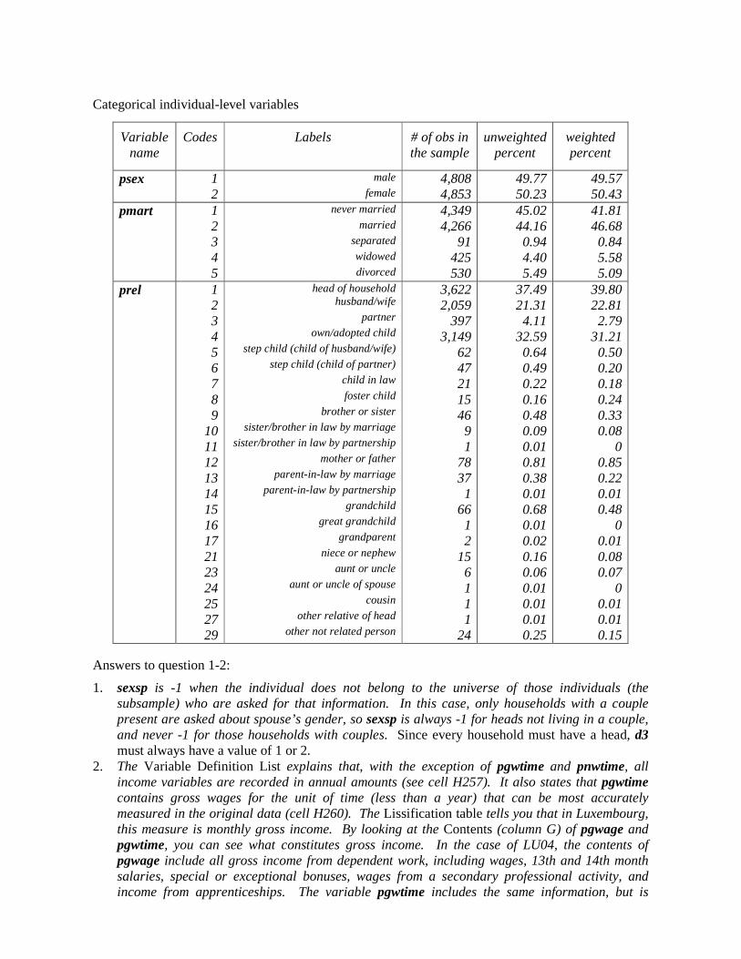
Categorical individual-level variables
Answers to question 1-2:
1. sexsp is -1 when the individual does not belong to the universe of those individuals (the subsample) who are asked for that information. In this case, only households with a couple present are asked about spouse’s gender, so sexsp is always -1 for heads not living in a couple, and never -1 for those households with couples. Since every household must have a head, d3 must always have a value of 1 or 2.
2. The Variable Definition List explains that, with the exception of pgwtime and pnwtime, all income variables are recorded in annual amounts (see cell H257). It also states that pgwtime contains gross wages for the unit of time (less than a year) that can be most accurately measured in the original data (cell H260). The Lissification table tells you that in Luxembourg, this measure is monthly gross income. By looking at the Contents (column G) of pgwage and pgwtime, you can see what constitutes gross income. In the case of LU04, the contents of pgwage include all gross income from dependent work, including wages, 13th and 14th month salaries, special or exceptional bonuses, wages from a secondary professional activity, and income from apprenticeships. The variable pgwtime includes the same information, but is
Variable name
Codes Labels # of obs in the sample
unweighted percent
weighted percent
psex 1 2
male
female 4,808 4,853
49.77 50.23
49.57 50.43
pmart 1 2 3 4 5
never married
married
separated
widowed
divorced
4,349 4,266
91 425 530
45.02 44.16 0.94 4.40 5.49
41.81 46.68 0.84 5.58 5.09
prel 1 2 3 4 5 6 7 8 9
10 11 12 13 14 15 16 17 21 23 24 25 27 29
head of household husband/wife
partner
own/adopted child
step child (child of husband/wife)
step child (child of partner)
child in law
foster child
brother or sister
sister/brother in law by marriage
sister/brother in law by partnership
mother or father
parent-in-law by marriage
parent-in-law by partnership
grandchild
great grandchild
grandparent
niece or nephew
aunt or uncle
aunt or uncle of spouse
cousin
other relative of head
other not related person
3,622 2,059
397 3,149
62 47 21 15 46 9 1
78 37 1
66 1 2
15 6 1 1 1
24
37.49 21.31 4.11
32.59 0.64 0.49 0.22 0.16 0.48 0.09 0.01 0.81 0.38 0.01 0.68 0.01 0.02 0.16 0.06 0.01 0.01 0.01 0.25
39.80 22.81 2.79
31.21 0.50 0.20 0.18 0.24 0.33 0.08
0 0.85 0.22 0.01 0.48
0 0.01 0.08 0.07
0 0.01 0.01 0.15
LAB SESSION BASICS I LIS Summer Workshop 2010
adjusted by the data provider to account for the number of months worked (e.g., if 2 individuals have the same value for pgwage, the individual with the fewest months worked will have a higher value for pgwtime.)
Comments
� File composition
There are 9,661 observations of the identifier, casenum, which gives us the total sample size (number of persons in this case).
Without opening the household-level files, we can get the total number of households in the sample by looking at the number of household heads (prel=1). In Luxembourg 2004, there are 3,622 household heads. In many cases, you can also find the number of households by looking at the maximum value of casenum (which here is also 3,622). If these two values differ, then some of the original households have been removed from the main file and have been either included in the shadow file or dropped completely. (Go to Luxembourg Income Study (LIS) � LIS Policy on the Treatment of Missing Information and Luxembourg Income Study (LIS) � LIS Policy on the Treatment of Shadow Files for a discussion about the LIS sample composition and shadow files.)
� Remember that the income variables are the nominal value of the national currency.
� Married variable
As of Wave V, pmart is always coded as 2 if married. If more detailed marital information is given by the data provider, never married will be coded as 1 and other marital information (e.g., divorced, separated, widowed) are given codes above 2.
Please be aware that when information about cohabiting status is not available for each person in the original dataset, a head with a cohabiting partner could be coded in pmart as single (if never civically married). See pparsta and prel for more information about cohabiting status.
� For this dataset, unweighted results on age (as well as other variables) are lower than the weighted ones. This means that younger individuals are over-represented in the sample. The sample (person) weight corrected for this by giving those individuals a lower weight. The unweighted result gives the average for the survey sample, not the Luxembourg average in 2004.
� Size of Population
For this dataset, the weight also inflates to total population. This means you can find the population size by looking at the “Sum of Wgt.” In the weighted summary.
- In some datasets, the average weight is equal to 1. In this case, the “Sum of Wgt.” Is equal to the number of observations in the sample.
- In other datasets, the weight “inflates to the population”, i.e. the weight for each unit in the sample is equal to the number of units he/she represents in the population (a “unit” could be a household or an individual). In other words, the average weight multiplied by the sample size gives the total population in the country.
� The person-level LIS weight is pweight. In some cases pweight is given directly by the data provider and is the inverse of the probability of the individual being included in the sample. In cases where pweight is not provided (e.g., most household surveys), pweight for each member in the household is equivalent to the household weight, hweight.

BASICS II
Ex. 3: Using Subroutines and Loops to Simplify Submissions Involving Several Datasets
Ex. 4: Combining Datasets

LAB SESSION BASICS II LIS Summer Workshop 2010
3. Using Subroutines and Loops to Simplify Submissions Involving Several Datasets
When doing comparative research, it is natural to want to run the same routine across several different countries or across different waves. This approach can be simplified by the use of macros, subprograms/subroutines, and loops. These are easy ways to repeat program commands without having to retype them each time.
Activity
Compare the median (weighted) labour earnings for the United States and Mexico (2000), and the United Kingdom (1999) by looking separately at gross wage earnings (pgwage), net wage earnings (pnwage) and self-employment earnings (pself). Your sample should only include those with positive labour earnings (from either paid or self-employment) who are 16 years of age or older. For this comparison, you should write a subroutine to run for each dataset.
Now repeat the same analysis for the five new Latin American datasets (BR06, CO04, GT06, PE04 and UY04). In order to shorten the code, loop the subroutine created above over the 5 datasets.
Use the information from your output to answer the following questions:
1. Which country had the highest median wages from employment?
_____________________________________________________________________________
_____________________________________________________________________________
_____________________________________________________________________________
2. Are the income variables analysed above expressed in net or gross terms (i.e. before or after deduction of income taxes and mandatory social contributions)?
_____________________________________________________________________________
_____________________________________________________________________________
_____________________________________________________________________________
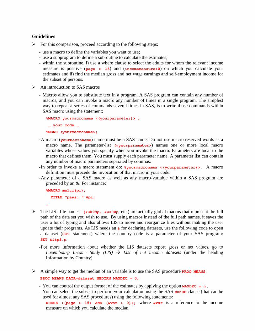
Guidelines
� For this comparison, proceed according to the following steps:
- use a macro to define the variables you want to use; - use a subprogram to define a subroutine to calculate the estimates; - within the subroutine, i) use a where clause to select the adults for whom the relevant income
measure is positive (page > 15 ) and (incomemeasure>0 ) on which you calculate your estimates and ii) find the median gross and net wage earnings and self-employment income for the subset of persons.
� An introduction to SAS macros
- Macros allow you to substitute text in a program. A SAS program can contain any number of macros, and you can invoke a macro any number of times in a single program. The simplest way to repeat a series of commands several times in SAS, is to write those commands within SAS macro using the statement:
%MACRO yourmacroname <(yourparameter)> ;
… your code …
%MEND <yourmacroname >;
- A macro (yourmacroname ) name must be a SAS name. Do not use macro reserved words as a macro name. The parameter-list (< yourparameter >) names one or more local macro variables whose values you specify when you invoke the macro. Parameters are local to the macro that defines them. You must supply each parameter name. A parameter list can contain any number of macro parameters separated by commas.
- In order to invoke a macro statement do: %yourmacroname <( yourparameter )>. A macro definition must precede the invocation of that macro in your code.
- Any parameter of a SAS macro as well as any macro-variable within a SAS program are preceded by an &. For instance:
%MACRO multi(pi);
TITLE “pays: “ π
…
� The LIS “file names” (&uk99p, &us00p , etc.) are actually global macros that represent the full path of the data set you wish to use. By using macros instead of the full path names, it saves the user a lot of typing and also allows LIS to move and reorganize files without making the user update their programs. As LIS needs an & for declaring datasets, use the following code to open a dataset (SET statement) where the country code is a parameter of your SAS program: SET &&&pi.p .
- For more information about whether the LIS datasets report gross or net values, go to Luxembourg Income Study (LIS) � List of net income datasets (under the heading Information by Country).
� A simple way to get the median of an variable is to use the SAS procedure PROC MEANS:
PROC MEANS DATA=dataset MEDIAN MAXDEC = 0;
- You can control the output format of the estimates by applying the option MAXDEC = n . - You can select the subset to perform your calculation using the SAS WHERE clause (that can be
used for almost any SAS procedures) using the following statements: WHERE ((page > 15) AND (&var > 0)); where &var is a reference to the income measure on which you calculate the median
LAB SESSION BASICS II LIS Summer Workshop 2010
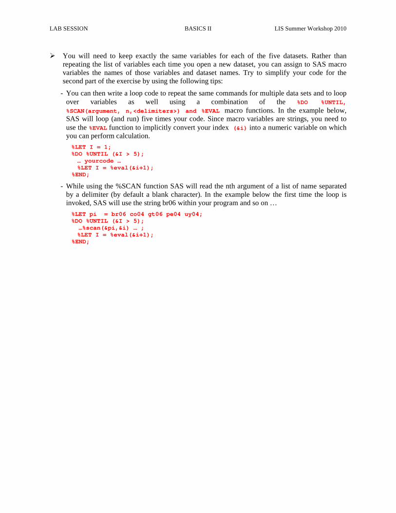
� You will need to keep exactly the same variables for each of the five datasets. Rather than repeating the list of variables each time you open a new dataset, you can assign to SAS macro variables the names of those variables and dataset names. Try to simplify your code for the second part of the exercise by using the following tips:
- You can then write a loop code to repeat the same commands for multiple data sets and to loop over variables as well using a combination of the %DO %UNTIL, %SCAN(argument, n,<delimiters>) and %EVAL macro functions. In the example below, SAS will loop (and run) five times your code. Since macro variables are strings, you need to use the %EVAL function to implicitly convert your index (&i) into a numeric variable on which you can perform calculation.
%LET I = 1; %DO %UNTIL (&I > 5); … yourcode …
%LET I = %eval(&i+1); %END;
- While using the %SCAN function SAS will read the nth argument of a list of name separated by a delimiter (by default a blank character). In the example below the first time the loop is invoked, SAS will use the string br06 within your program and so on …
%LET pi = br06 co04 gt06 pe04 uy04; %DO %UNTIL (&I > 5); …%scan(&pi,&i) … ;
%LET I = %eval(&i+1); %END;
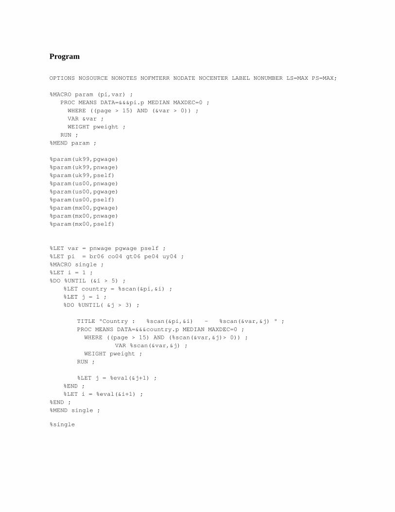
Program
OPTIONS NOSOURCE NONOTES NOFMTERR NODATE NOCENTER LABEL NONUMBER LS=MAX PS=MAX;
%MACRO param (pi,var) ;
PROC MEANS DATA=&&&pi.p MEDIAN MAXDEC=0 ;
WHERE ((page > 15) AND (&var > 0)) ;
VAR &var ;
WEIGHT pweight ;
RUN ;
%MEND param ;
%param(uk99,pgwage)
%param(uk99,pnwage)
%param(uk99,pself)
%param(us00,pnwage)
%param(us00,pgwage)
%param(us00,pself)
%param(mx00,pgwage)
%param(mx00,pnwage)
%param(mx00,pself)
%LET var = pnwage pgwage pself ;
%LET pi = br06 co04 gt06 pe04 uy04 ;
%MACRO single ;
%LET i = 1 ;
%DO %UNTIL (&i > 5) ;
%LET country = %scan(&pi,&i) ;
%LET j = 1 ;
%DO %UNTIL( &j > 3) ;
TITLE "Country : %scan(&pi,&i) – %scan(&var ,&j) " ;
PROC MEANS DATA=&&&country.p MEDIAN MAXDEC=0 ;
WHERE ((page > 15) AND (%scan(&var,&j)> 0)) ;
VAR %scan(&var,&j) ;
WEIGHT pweight ;
RUN ;
%LET j = %eval(&j+1) ;
%END ;
%LET i = %eval(&i+1) ;
%END ;
%MEND single ;
%single
LAB SESSION BASICS II LIS Summer Workshop 2010
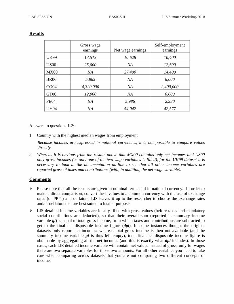
Results
Gross wage earnings Net wage earnings
Self-employment earnings
UK99 13,513 10,628 10,400
US00 25,000 NA 12,500
MX00 NA 27,400 14,400
BR06 5,865 NA 6,000
CO04 4,320,000 NA 2,400,000
GT06 12,000 NA 6,000
PE04 NA 5,986 2,980
UY04 NA 54,042 42,577
Answers to questions 1-2:
1. Country with the highest median wages from employment
Because incomes are expressed in national currencies, it is not possible to compare values directly.
2. Whereas it is obvious from the results above that MX00 contains only net incomes and US00 only gross incomes (as only one of the two wage variables is filled), for the UK99 dataset it is necessary to look at the documentation on-line to see that all other income variables are reported gross of taxes and contributions (with, in addition, the net wage variable).
Comments
� Please note that all the results are given in nominal terms and in national currency. In order to make a direct comparison, convert these values to a common currency with the use of exchange rates (or PPPs) and deflators. LIS leaves it up to the researcher to choose the exchange rates and/or deflators that are best suited to his/her purpose.
� LIS detailed income variables are ideally filled with gross values (before taxes and mandatory social contributions are deducted), so that their overall sum (reported in summary income variable gi) is equal to total gross income, from which taxes and contributions are subtracted to get to the final net disposable income figure (dpi). In some instances though, the original datasets only report net incomes: whereas total gross income is then not available (and the summary income variable gi is thus left empty), total final net disposable income figure is obtainable by aggregating all the net incomes (and this is exactly what dpi includes). In those cases, each LIS detailed income variable will contain net values instead of gross; only for wages there are two separate variables for those two amounts. For all other variables you need to take care when comparing across datasets that you are not comparing two different concepts of income.

LAB SESSION BASICS II LIS Summer Workshop 2010
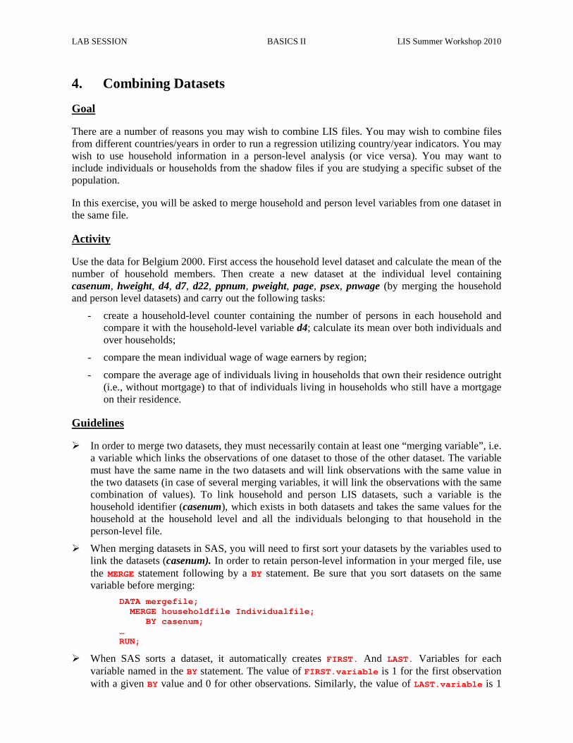
4. Combining Datasets
Goal
There are a number of reasons you may wish to combine LIS files. You may wish to combine files from different countries/years in order to run a regression utilizing country/year indicators. You may wish to use household information in a person-level analysis (or vice versa). You may want to include individuals or households from the shadow files if you are studying a specific subset of the population.
In this exercise, you will be asked to merge household and person level variables from one dataset in the same file.
Activity
Use the data for Belgium 2000. First access the household level dataset and calculate the mean of the number of household members. Then create a new dataset at the individual level containing casenum, hweight, d4, d7, d22, ppnum, pweight, page, psex, pnwage (by merging the household and person level datasets) and carry out the following tasks:
- create a household-level counter containing the number of persons in each household and compare it with the household-level variable d4; calculate its mean over both individuals and over households;
- compare the mean individual wage of wage earners by region;
- compare the average age of individuals living in households that own their residence outright (i.e., without mortgage) to that of individuals living in households who still have a mortgage on their residence.
Guidelines
� In order to merge two datasets, they must necessarily contain at least one “merging variable”, i.e. a variable which links the observations of one dataset to those of the other dataset. The variable must have the same name in the two datasets and will link observations with the same value in the two datasets (in case of several merging variables, it will link the observations with the same combination of values). To link household and person LIS datasets, such a variable is the household identifier (casenum), which exists in both datasets and takes the same values for the household at the household level and all the individuals belonging to that household in the person-level file.
� When merging datasets in SAS, you will need to first sort your datasets by the variables used to link the datasets (casenum). In order to retain person-level information in your merged file, use the MERGE statement following by a BY statement. Be sure that you sort datasets on the same variable before merging:
DATA mergefile ; MERGE householdfile Individualfile ; BY casenum; … RUN;
� When SAS sorts a dataset, it automatically creates FIRST. And LAST. Variables for each variable named in the BY statement. The value of FIRST. variable is 1 for the first observation with a given BY value and 0 for other observations. Similarly, the value of LAST. variable is 1
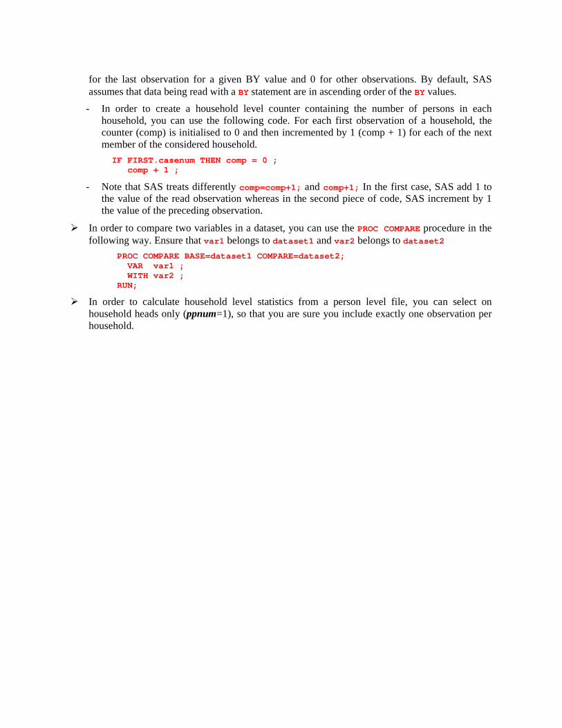
for the last observation for a given BY value and 0 for other observations. By default, SAS assumes that data being read with a BY statement are in ascending order of the BY values.
- In order to create a household level counter containing the number of persons in each household, you can use the following code. For each first observation of a household, the counter (comp) is initialised to 0 and then incremented by 1 (comp + 1) for each of the next member of the considered household.
IF FIRST.casenum THEN comp = 0 ; comp + 1 ;
- Note that SAS treats differently comp=comp+1; and comp+1; In the first case, SAS add 1 to the value of the read observation whereas in the second piece of code, SAS increment by 1 the value of the preceding observation.
� In order to compare two variables in a dataset, you can use the PROC COMPARE procedure in the following way. Ensure that var1 belongs to dataset1 and var2 belongs to dataset2
PROC COMPARE BASE=dataset1 COMPARE=dataset2 ; VAR var1 ; WITH var2 ; RUN;
� In order to calculate household level statistics from a person level file, you can select on household heads only (ppnum=1), so that you are sure you include exactly one observation per household.
LAB SESSION BASICS II LIS Summer Workshop 2010
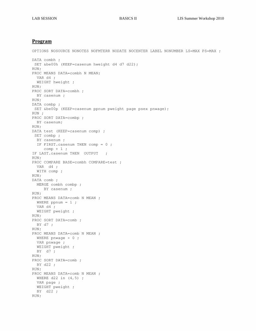
Program
OPTIONS NOSOURCE NONOTES NOFMTERR NODATE NOCENTER LABEL NONUMBER LS=MAX PS=MAX ; DATA combh ; SET &be00h (KEEP=casenum hweight d4 d7 d22); RUN; PROC MEANS DATA=combh N MEAN; VAR d4 ; WEIGHT hweight ; RUN; PROC SORT DATA=combh ; BY casenum ; RUN; DATA combp ; SET &be00p (KEEP=casenum ppnum pweight page psex p nwage); RUN ; PROC SORT DATA=combp ; BY casenum; RUN; DATA test (KEEP=casenum comp) ; SET combp ; BY casenum ; IF FIRST.casenum THEN comp = 0 ; comp + 1 ; IF LAST.casenum THEN OUTPUT ; RUN; PROC COMPARE BASE=combh COMPARE=test ; VAR d4 ; WITH comp ; RUN; DATA comb ; MERGE combh combp ; BY casenum ; RUN; PROC MEANS DATA=comb N MEAN ; WHERE ppnum = 1 ; VAR d4 ; WEIGHT pweight ; RUN; PROC SORT DATA=comb ; BY d7 ; RUN; PROC MEANS DATA=comb N MEAN ; WHERE pnwage > 0 ; VAR pnwage ; WEIGHT pweight ; BY d7 ; RUN; PROC SORT DATA=comb ; BY d22 ; RUN; PROC MEANS DATA=comb N MEAN ; WHERE d22 in (4,5) ; VAR page ; WEIGHT pweight ; BY d22 ; RUN;
Results
Comments
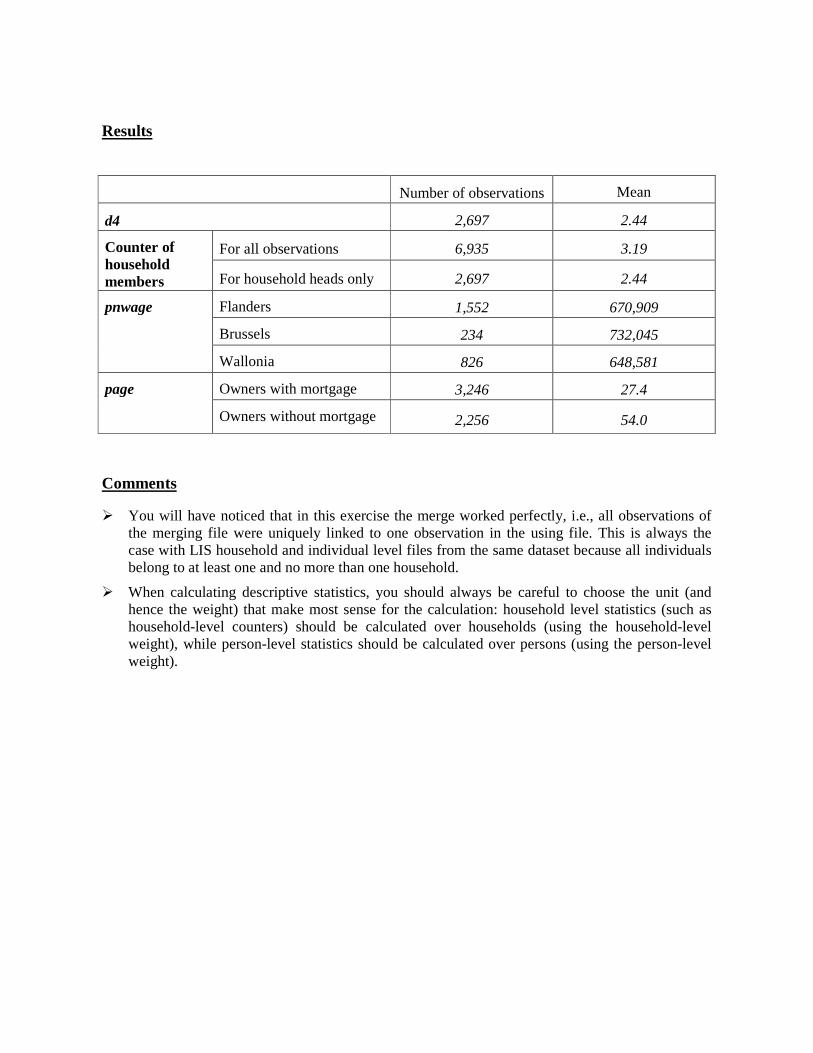
� You will have noticed that in this exercise the merge worked perfectly, i.e., all observations of the merging file were uniquely linked to one observation in the using file. This is always the case with LIS household and individual level files from the same dataset because all individuals belong to at least one and no more than one household.
� When calculating descriptive statistics, you should always be careful to choose the unit (and hence the weight) that make most sense for the calculation: household level statistics (such as household-level counters) should be calculated over households (using the household-level weight), while person-level statistics should be calculated over persons (using the person-level weight).
Number of observations Mean
d4 2,697 2.44
Counter of household members
For all observations 6,935 3.19
For household heads only 2,697 2.44
pnwage Flanders 1,552 670,909
Brussels 234 732,045
Wallonia 826 648,581
page Owners with mortgage 3,246 27.4
Owners without mortgage 2,256 54.0

DEMOGRAPHICS AND EDUCATION
Ex. 5: Children (Household Level)
Ex. 6: Gender (Person Level)
Ex. 7: Comparing educ and peduc
Ex. 8: Comparing Educational Outcomes

LAB SESSION DEMOGRAPHICS AND EDUCATION LIS Summer Workshop 2010
5. Children (Household Level)
Goal
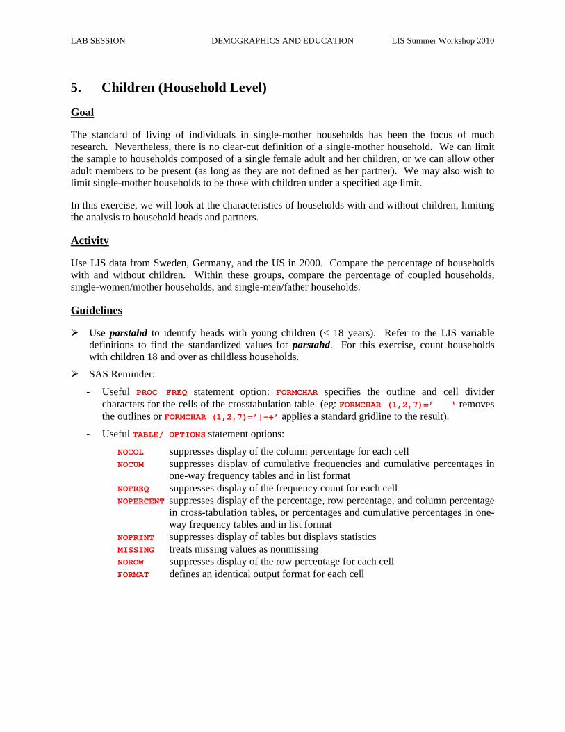
The standard of living of individuals in single-mother households has been the focus of much research. Nevertheless, there is no clear-cut definition of a single-mother household. We can limit the sample to households composed of a single female adult and her children, or we can allow other adult members to be present (as long as they are not defined as her partner). We may also wish to limit single-mother households to be those with children under a specified age limit.
In this exercise, we will look at the characteristics of households with and without children, limiting the analysis to household heads and partners.
Activity
Use LIS data from Sweden, Germany, and the US in 2000. Compare the percentage of households with and without children. Within these groups, compare the percentage of coupled households, single-women/mother households, and single-men/father households.
Guidelines
� Use parstahd to identify heads with young children (< 18 years). Refer to the LIS variable definitions to find the standardized values for parstahd. For this exercise, count households with children 18 and over as childless households.
� SAS Reminder:
- Useful PROC FREQ statement option: FORMCHAR specifies the outline and cell divider characters for the cells of the crosstabulation table. (eg: FORMCHAR (1,2,7)=’ ‘ removes the outlines or FORMCHAR (1,2,7)=’|-+’ applies a standard gridline to the result).
- Useful TABLE/ OPTIONS statement options:
NOCOL suppresses display of the column percentage for each cell NOCUM suppresses display of cumulative frequencies and cumulative percentages in
one-way frequency tables and in list format NOFREQ suppresses display of the frequency count for each cell NOPERCENT suppresses display of the percentage, row percentage, and column percentage
in cross-tabulation tables, or percentages and cumulative percentages in one-way frequency tables and in list format
NOPRINT suppresses display of tables but displays statistics MISSING treats missing values as nonmissing NOROW suppresses display of the row percentage for each cell FORMAT defines an identical output format for each cell
Program
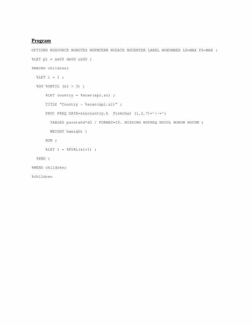
OPTIONS NOSOURCE NONOTES NOFMTERR NODATE NOCENTER LABEL NONUMBER LS=MAX PS=MAX ;
%LET pi = se00 de00 us00 ;
%MACRO children;
%LET i = 1 ;
%DO %UNTIL (&i > 3) ;
%LET country = %scan(&pi,&i) ;
TITLE “Country – %scan(&pi,&i)” ;
PROC FREQ DATA=&&&country.h formchar (1,2,7) ='|-+';
TABLES parstahd*d3 / FORMAT=10. MISSING NOF REQ NOCOL NOROW NOCUM ;
WEIGHT hweight ;
RUN ;
%LET i = %EVAL(&i+1) ;
%END ;
%MEND children;
%children
LAB SESSION DEMOGRAPHICS AND EDUCATION LIS Summer Workshop 2010
Results
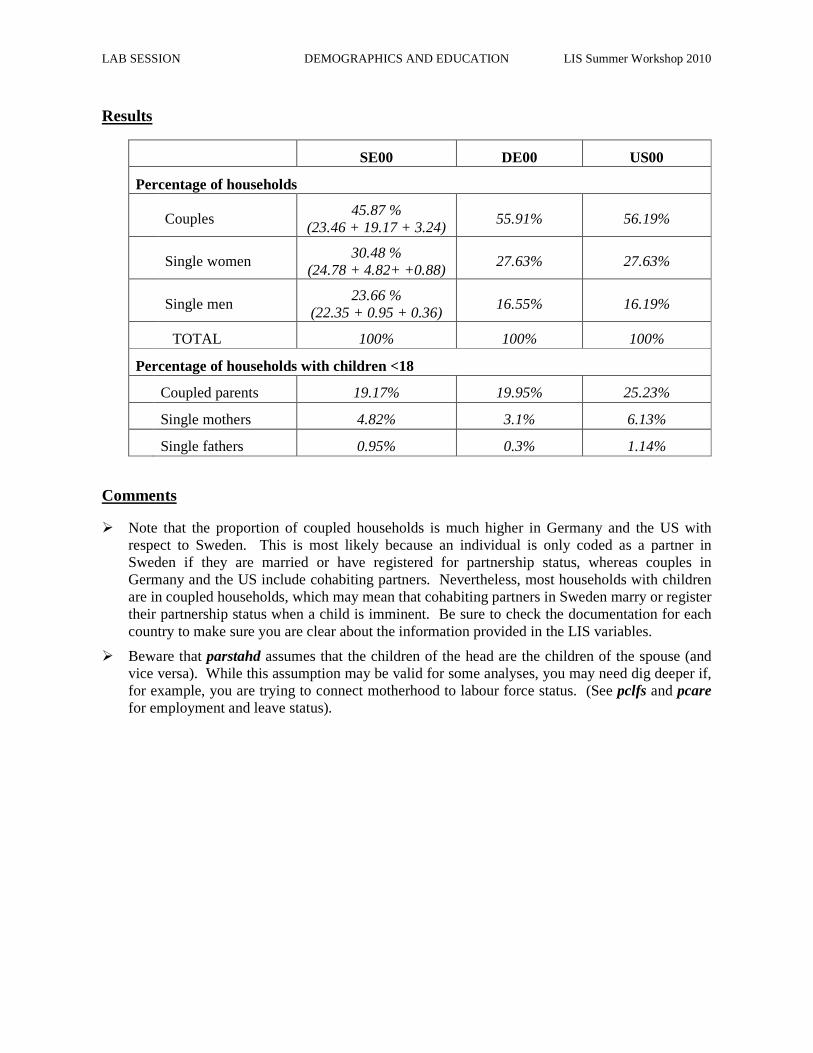
SE00 DE00 US00
Percentage of households
Couples 45.87 %
(23.46 + 19.17 + 3.24) 55.91% 56.19%
Single women 30.48 %
(24.78 + 4.82+ +0.88) 27.63% 27.63%
Single men 23.66 %
(22.35 + 0.95 + 0.36) 16.55% 16.19%
TOTAL 100% 100% 100%
Percentage of households with children <18
Coupled parents 19.17% 19.95% 25.23%
Single mothers 4.82% 3.1% 6.13%
Single fathers 0.95% 0.3% 1.14%
Comments
� Note that the proportion of coupled households is much higher in Germany and the US with respect to Sweden. This is most likely because an individual is only coded as a partner in Sweden if they are married or have registered for partnership status, whereas couples in Germany and the US include cohabiting partners. Nevertheless, most households with children are in coupled households, which may mean that cohabiting partners in Sweden marry or register their partnership status when a child is imminent. Be sure to check the documentation for each country to make sure you are clear about the information provided in the LIS variables.
� Beware that parstahd assumes that the children of the head are the children of the spouse (and vice versa). While this assumption may be valid for some analyses, you may need dig deeper if, for example, you are trying to connect motherhood to labour force status. (See pclfs and pcare for employment and leave status).

LAB SESSION DEMOGRAPHICS AND EDUCATION LIS Summer Workshop 2010
6. Gender (Person Level)
Goal
In doing any estimation, it is important to be careful about the unit of analysis. In research focusing on women, you must take into account whether the data you are using are individual- or household-specific.
Using individual-level data allows you to identify individual-specific income, but problems may arise in estimation depending on your research question. Some of these issues are general, but others are specific to the LIS database. First, some income sources are common to the household (such as child benefits or housing allowances) and are not available at the individual level. In LIS, certain individual income sources (invalidity and work accident pensions, sickness and maternity allowances, means-tested benefits, social transfers) are reported in detail only in the household file. The information is present in the person-level file in an aggregated form.
In this exercise, we introduce income analysis by gender. Using the person-level file, we will focus only on earned income amounts, not considering social transfers.
Activity
Examine the working-aged population (25 to 60, inclusive) in the UK in 1999 and the US in 2000. Compare the percentage of working men to that of working women (defined as those with positive earnings from any employment). Calculate the average total income by gender of both the total working-aged population and the working population. Estimate the gender earnings gap for both the working-aged population and for those who work.
Guidelines
� For this exercise, define the “working-aged” population as those aged 25 to 60, inclusive, and the “working” population as those with positive earnings from paid and/or self-employment (pgwage + pself).
� The gender income gap is defined as the ratio of average total earnings (pgwage+pself) of males to females.
� To simplify the analysis in this exercise, set negative values of pself to missing before calculating the “working” population. Failure to do so may result in self-employed with negative incomes being counted as not working, or negative incomes being considered in the average for the population.
� SAS reminder:
- Only keep the variables you will be using. This avoids unnecessary burden on the machine so that submitted jobs will run faster.
(KEEP=casenum d6 d27 married d1 d3 dpi);
- To keep observations that pertain to a certain group of persons, use the statement IF <expression> . The expression is assessed by SAS as a Boolean (getting the value either true or false). Only observations that receive a true assessment are kept.
- IF ((page>15) AND (pgwage>0)); this expression allows you to select earners. - IF condition THEN action ;
<ELSE action ;>
This piece of code tests whether the condition is true; if so, the action in the THEN clause is carried out. If the condition is false and an ELSE statement is present, then the ELSE action is carried out. If the condition is false and no ELSE statement is present, then the next statement in the DATA step is processed. The condition is one or more numeric or character comparisons. The action must be an executable statement; that is, one that can be processed in an individual iteration of the DATA step. In SAS processing, any numeric value other than 0 or missing is true; 0 and missing are false. Therefore, a numeric value can stand alone in a comparison. If its value is 0 or missing, then the comparison is false; otherwise, the comparison is true.
- Useful PROC MEANS statement options:
SUMWGT Calculate separate statistics for each BY group MISSING Use missing values as valid values to create combinations of class variables
- Useful PROC MEANS statements:
BY Calculate separate statistics for each BY group CLASS Identify variables whose values define subgroups for the analysis TYPES Identify specific combinations of class variables to use to subdivide the data
PROC MEANS DATA=youroutput MEAN SUMWGT MISSING; CLASS wap wp psex; TYPES wap*psex wp*psex ; VAR yourtotalincome ; WEIGHT pweight; RUN ;
Where the dummy variable wap represents the “working-aged population” and wp the ”working population” for instance.
LAB SESSION DEMOGRAPHICS AND EDUCATION LIS Summer Workshop 2010
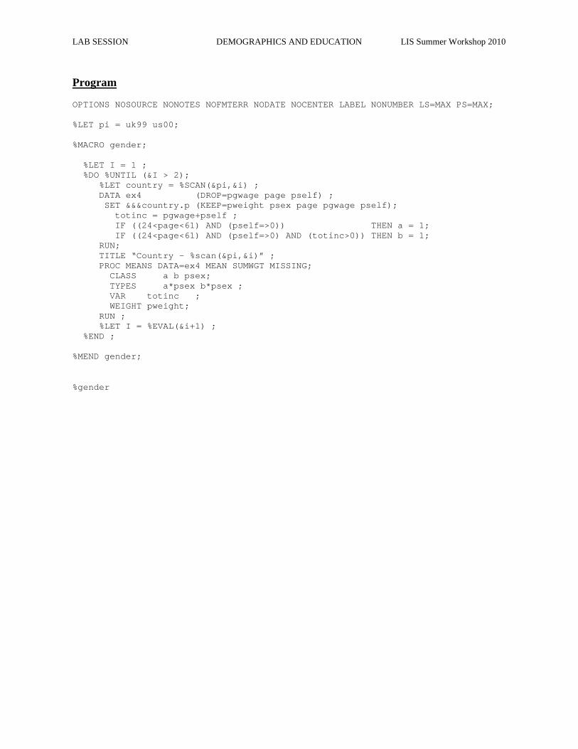
Program
OPTIONS NOSOURCE NONOTES NOFMTERR NODATE NOCENTER LABEL NONUMBER LS=MAX PS=MAX; %LET pi = uk99 us00; %MACRO gender; %LET I = 1 ; %DO %UNTIL (&I > 2); %LET country = %SCAN(&pi,&i) ; DATA ex4 (DROP=pgwage page pself) ; SET &&&country.p (KEEP=pweight psex page pgwa ge pself); totinc = pgwage+pself ; IF ((24<page<61) AND (pself=>0)) THEN a = 1; IF ((24<page<61) AND (pself=>0) AND (totinc >0)) THEN b = 1; RUN; TITLE “Country – %scan(&pi,&i)” ; PROC MEANS DATA=ex4 MEAN SUMWGT MISSING; CLASS a b psex; TYPES a*psex b*psex ; VAR totinc ; WEIGHT pweight; RUN ; %LET I = %EVAL(&i+1) ; %END ; %MEND gender;
%gender
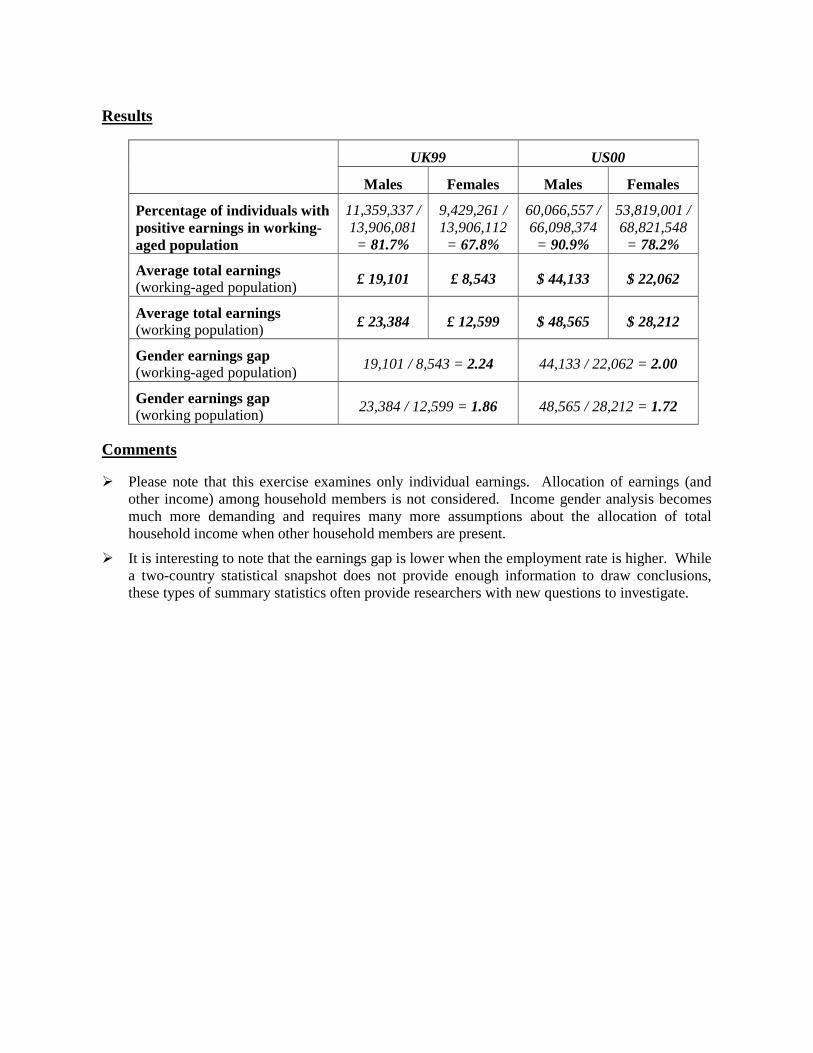
Results
UK99 US00
Males Females Males Females
Percentage of individuals with positive earnings in working-aged population
11,359,337 / 13,906,081 = 81.7%
9,429,261 / 13,906,112 = 67.8%
60,066,557 / 66,098,374 = 90.9%
53,819,001 / 68,821,548 = 78.2%
Average total earnings (working-aged population) £ 19,101 £ 8,543 $ 44,133 $ 22,062
Average total earnings (working population) £ 23,384 £ 12,599 $ 48,565 $ 28,212
Gender earnings gap (working-aged population)
19,101 / 8,543 = 2.24 44,133 / 22,062 = 2.00
Gender earnings gap (working population)
23,384 / 12,599 = 1.86 48,565 / 28,212 = 1.72
Comments
� Please note that this exercise examines only individual earnings. Allocation of earnings (and other income) among household members is not considered. Income gender analysis becomes much more demanding and requires many more assumptions about the allocation of total household income when other household members are present.
� It is interesting to note that the earnings gap is lower when the employment rate is higher. While a two-country statistical snapshot does not provide enough information to draw conclusions, these types of summary statistics often provide researchers with new questions to investigate.
LAB SESSION DEMOGRAPHICS AND EDUCATION LIS Summer Workshop 2010
7. Comparing educ and peduc
Goal
Education information can vary substantially between datasets. This results mainly from the different educational systems in the various countries, but can also be the result of different ways of surveying the topic. (Some surveys allow for very detailed answers, while others ask only for categories of education). LIS harmonises, but does not standardise this information; that is, the original survey information is coded into the same variable for every country, but as much country-specific detail as possible remains.
Nevertheless, since measures of comparable education are used in many areas of research, LIS has created a standardisation routine for the education variables that transforms each country-specific educational label into a new standardised variable based on the International Standard Classification of Education (ISCED). This exercise compares the country-specific education information to the ISCED recoding using that routine.
Activity
Using data from the United States and Luxembourg in 2000, run the education recode program to create the standardized education variable (educ). Tabulate the country-specific education variable (peduc) with the LIS standardized education variable (educ).
Guidelines
� When running the education recode file, remember to include the variables country, ptocc, and peduc when calling your country file.
� To run the education standardization program, include the following line in your program:
%include “&myincl.educrecodepp.sas”;
� For more information about how education levels are recoded in each country, see http://www.lisproject.org/techdoc/education-level/education-level.htm.
� To compare peduc and educ, use a PROC FREQ procedure.
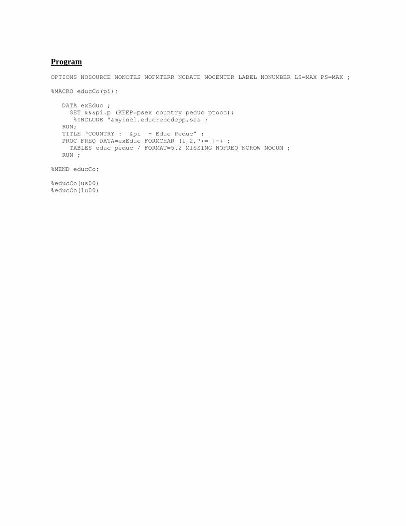
Program
OPTIONS NOSOURCE NONOTES NOFMTERR NODATE NOCENTER LABEL NONUMBER LS=MAX PS=MAX ; %MACRO educCo(pi); DATA exEduc ; SET &&&pi.p (KEEP=psex country peduc ptocc); %INCLUDE "&myincl.educrecodepp.sas"; RUN; TITLE “COUNTRY : &pi – Educ Peduc” ; PROC FREQ DATA=exEduc FORMCHAR (1,2,7)='|-+'; TABLES educ peduc / FORMAT=5.2 MISSING NOFREQ NOROW NOCUM ; RUN ; %MEND educCo; %educCo(us00) %educCo(lu00)
LAB SESSION DEMOGRAPHICS AND EDUCATION LIS Summer Workshop 2010
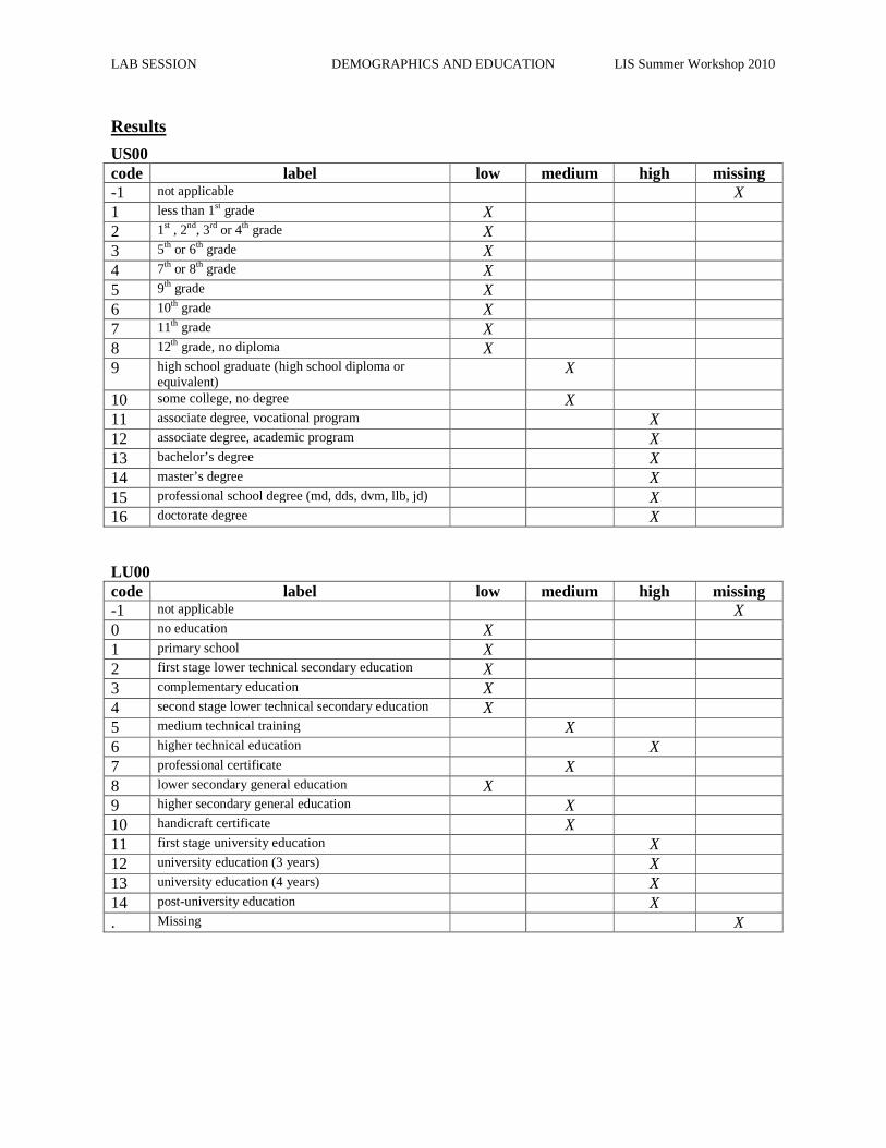
Results
US00 code label low medium high missing -1 not applicable X 1 less than 1st grade X 2 1st , 2nd, 3rd or 4th grade X 3 5th or 6th grade X 4 7th or 8th grade X 5 9th grade X 6 10th grade X 7 11th grade X 8 12th grade, no diploma X 9 high school graduate (high school diploma or
equivalent) X
10 some college, no degree X 11 associate degree, vocational program X 12 associate degree, academic program X 13 bachelor’s degree X 14 master’s degree X 15 professional school degree (md, dds, dvm, llb, jd) X 16 doctorate degree X
LU00 code label low medium high missing -1 not applicable X 0 no education X 1 primary school X 2 first stage lower technical secondary education X 3 complementary education X 4 second stage lower technical secondary education X 5 medium technical training X 6 higher technical education X 7 professional certificate X 8 lower secondary general education X 9 higher secondary general education X 10 handicraft certificate X 11 first stage university education X 12 university education (3 years) X 13 university education (4 years) X 14 post-university education X . Missing X

LAB SESSION DEMOGRAPHICS AND EDUCATION LIS Summer Workshop 2010
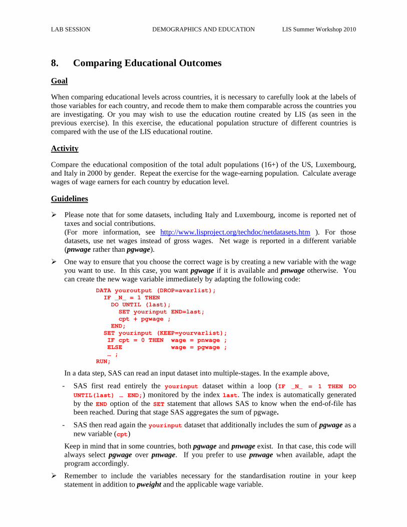
8. Comparing Educational Outcomes
Goal
When comparing educational levels across countries, it is necessary to carefully look at the labels of those variables for each country, and recode them to make them comparable across the countries you are investigating. Or you may wish to use the education routine created by LIS (as seen in the previous exercise). In this exercise, the educational population structure of different countries is compared with the use of the LIS educational routine.
Activity
Compare the educational composition of the total adult populations (16+) of the US, Luxembourg, and Italy in 2000 by gender. Repeat the exercise for the wage-earning population. Calculate average wages of wage earners for each country by education level.
Guidelines
� Please note that for some datasets, including Italy and Luxembourg, income is reported net of taxes and social contributions. (For more information, see http://www.lisproject.org/techdoc/netdatasets.htm ). For those datasets, use net wages instead of gross wages. Net wage is reported in a different variable (pnwage rather than pgwage).
� One way to ensure that you choose the correct wage is by creating a new variable with the wage you want to use. In this case, you want pgwage if it is available and pnwage otherwise. You can create the new wage variable immediately by adapting the following code:
DATA youroutput (DROP=avarlist ); IF _N_ = 1 THEN DO UNTIL (last); SET yourinput END=last; cpt + pgwage ; END; SET yourinput (KEEP= yourvarlist ); IF cpt = 0 THEN wage = pnwage ; ELSE wage = pgwage ; … ; RUN;
In a data step, SAS can read an input dataset into multiple-stages. In the example above,
- SAS first read entirely the yourinput dataset within a loop (IF _N_ = 1 THEN DO UNTIL(last) … END; ) monitored by the index last . The index is automatically generated by the END option of the SET statement that allows SAS to know when the end-of-file has been reached. During that stage SAS aggregates the sum of pgwage.
- SAS then read again the yourinput dataset that additionally includes the sum of pgwage as a new variable (cpt )
Keep in mind that in some countries, both pgwage and pnwage exist. In that case, this code will always select pgwage over pnwage. If you prefer to use pnwage when available, adapt the program accordingly.
� Remember to include the variables necessary for the standardisation routine in your keep statement in addition to pweight and the applicable wage variable.
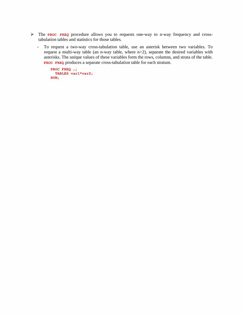
� The PROC FREQ procedure allows you to requests one-way to n-way frequency and cross-tabulation tables and statistics for those tables.
- To request a two-way cross-tabulation table, use an asterisk between two variables. To request a multi-way table (an n-way table, where n>2), separate the desired variables with asterisks. The unique values of these variables form the rows, columns, and strata of the table. PROC FREQ produces a separate cross-tabulation table for each stratum.
PROC FREQ …; TABLES var1*var2 ; RUN;
LAB SESSION DEMOGRAPHICS AND EDUCATION LIS Summer Workshop 2010
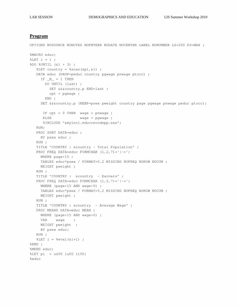
Program
OPTIONS NOSOURCE NONOTES NOFMTERR NODATE NOCENTER LABEL NONUMBER LS=200 PS=MAX ;
%MACRO educ;
%LET i = 1 ;
%DO %UNTIL (&i > 3) ;
%LET country = %scan(&pi,&i) ;
DATA educ (DROP=peduc country pgwage pnwage ptoc c) ;
IF _N_ = 1 THEN
DO UNTIL (last) ;
SET &&&country.p END=last ;
cpt + pgwage ;
END ;
SET &&&country.p (KEEP=psex pweight country pa ge pgwage pnwage peduc ptocc);
IF cpt = 0 THEN wage = pnwage ;
ELSE wage = pgwage ;
%INCLUDE "&myincl.educrecodepp.sas";
RUN;
PROC SORT DATA=educ ;
BY psex educ ;
RUN ;
TITLE "COUNTRY : &country - Total Population" ;
PROC FREQ DATA=educ FORMCHAR (1,2,7)='|-+';
WHERE page>15 ;
TABLES educ*psex / FORMAT=5.2 MISSING NOFREQ N OROW NOCUM ;
WEIGHT pweight ;
RUN ;
TITLE "COUNTRY : &country - Earners" ;
PROC FREQ DATA=educ FORMCHAR (1,2,7)='|-+';
WHERE (page>15 AND wage>0) ;
TABLES educ*psex / FORMAT=5.2 MISSING NOFREQ N OROW NOCUM ;
WEIGHT pweight ;
RUN ;
TITLE "COUNTRY : &country - Average Wage" ;
PROC MEANS DATA=educ MEAN ;
WHERE (page>15 AND wage>0) ;
VAR wage ;
WEIGHT pweight ;
BY psex educ;
RUN ;
%LET i = %eval(&i+1) ;
%END ;
%MEND educ;
%LET pi = us00 lu00 it00;
%educ
Results
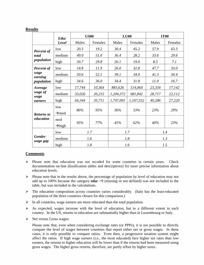
Educ Level
US00 LU00 IT00
Males Females Males Females Males Females
Percent of total population
low 20.3 19.2 30.4 45.2 57.9 63.3
medium 49.0 51.0 36.4 28.2 33.6 29.6
high 30.7 29.8 26.1 19.0 8.5 7.1
Percent of wage earning population
low 14.8 11.9 26.0 32.8 47.7 33.0
medium 50.6 52.1 39.1 34.9 41.3 50.4
high 34.6 36.0 34.4 31.8 11.0 16.7
Average wage of wage earners
low 17,744 10,364 883,626 514,064 23,334 17,142
medium 33,026 20,215 1,204,372 681,842 28,717 22,112
high 64,344 35,711 1,747,091 1,107,552 40,286 27,220
Returns to education
low
�med 86% 95% 36% 33% 23% 29%
med
�high 95% 77% 45% 62% 40% 23%
Gender wage gap
low 1.7 1.7 1.4
medium 1.6 1.8 1.3
high 1.8 1.6 1.5
Comments
� Please note that education was not recoded for some countries in certain years. Check documentation on-line (lissification tables and descriptives) for more precise information about education levels.
� Please note that in the results above, the percentage of population by level of education may not add up to 100% because the category educ =9 (missing or not defined) was not included in the table, but was included in the calculations.
� The education composition across countries varies considerably. (Italy has the least-educated population of the three countries chosen for this comparison.)
� In all countries, wage earners are more educated than the total population.
� As expected, wages increase with the level of education, but to a different extent in each country. In the US, returns to education are substantially higher than in Luxembourg or Italy.
� Net versus Gross wages:
Please note that, even when considering exchange rates (or PPPs), it is not possible to directly compare the level of wages between countries that report either net or gross wages. In these cases, it is only possible to compare ratios. Even then, a progressive taxation system might affect the ratios. If high wage earners (i.e., the most educated) face higher tax rates than low earners, the returns to higher education will be lower than if the returns had been measured using gross wages. The higher gross returns, therefore, are partly offset by higher taxes.
INCOME DISTRIBUTION I
Ex. 9: Equivalence Scales
Ex. 10: Poverty Lines and Poverty Rates
Ex. 11: Elderly and Child Poverty Rates

LAB SESSION INCOME DISTRIBUTION I LIS Summer Workshop 2010
9. Equivalence Scales
Goal
In order to get measures of poverty and/or income inequality in a population, it is necessary to compare income across different types of households. It is not logical to directly compare total household income between households of different sizes and composition.
Suppose you observe three levels of income (A, B, and C), where A>B>C. You cannot state that a household earning A is better off than one earning B unless you know the two households are similar in composition. For example, a family of 4 adult members receiving A is not necessarily better off than a couple with 2 children who receive B, and the family receiving B may not be better off than the childless couple receiving C.
For this reason, total household income needs to be adjusted to make it comparable across different households. This exercise gives one example of “equalizing” households using one specific equivalence scale.
Activity
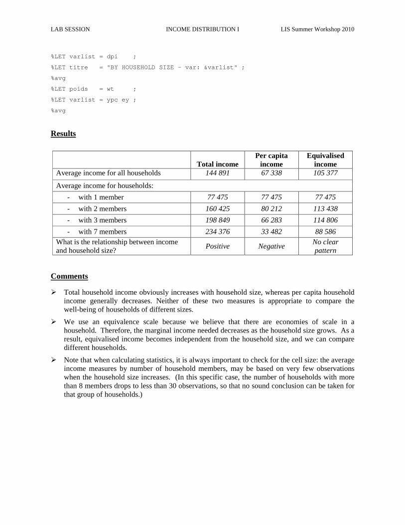
Summarise total disposable income, per capita disposable income, and equivalised disposable income using the “LIS equivalence scale” (i.e., the square root of the number of household members) in Finland in 2000. First calculate the averages for the total population. Then recalculate the same averages by the number of household members. Print your results only for households with 7 or fewer household members. Be sure to eliminate observations with zero or missing dpi and to use the appropriate weights.
Guidelines
� Do not forget to “clean” the data. As always, it is important to be vigilant about missing values. Prior to Wave V, no distinction was made between 0 and missing values. Starting from Wave V, the lissification process consistently coded missing values with a “dot” and genuine 0 values by 0. Nevertheless, to be able to cover all the waves consistently we advise you to drop both missing and 0 values of dpi.
Warning! When you start working with smaller sub-samples, dropping observations may significantly affect your results if dropped observations all belong to one group that is central to your analysis (e.g., older immigrants, or low-educated blue-collar workers). Be careful about what you are doing. Understand your data.
� To equivalise income, divide the total household income by the value of the equivalence scale for each observation. To generate LIS equivalised income:
ey = dpi /SQRT(d4);
� Be careful when using weights. Make sure that the weight matches your unit of analysis. Weigh by hweight for variables which are intrinsically at the household level (e.g., dpi) and by hweight*d4 (to account for household size) for variables that are conceptually meaningful at the person level (e.g., per capita and equivalised income).
Program
OPTIONS NONOTES NOSOURCE NOFMTERR NODATE NONUMBER NOCENTER LABEL LS=MAX PS=MAX;
/** MACRO DECLARATION **/
%MACRO avg ;
TITLE &titre ;
PROC MEANS DATA=eq MEAN;
&where ;
&by ;
WEIGHT &poids ;
VAR &varlist ;
RUN;
%MEND avg ;
/** START PROGRAM **/
DATA eq ;
SET &fi00h (KEEP=casenum hweight d4 dpi);
* Cleaning data;
IF dpi in (. 0) THEN DELETE;
* Income per capita;
ypc = dpi / d4;
* Equivalised income;
ey = dpi /SQRT(d4);
* Individual weight;
wt=hweight * d4 ;
RUN;
PROC SORT DATA=eq;
BY d4;
RUN;
%LET where ;
%LET by ;
%LET poids = hweight ;
%LET varlist = dpi ;
%LET titre = "TOTAL POPULATION - var: &varlist" ;
%avg
%LET poids = wt ;
%LET varlist = ypc ey ;
%avg
%LET where = WHERE d4 LE 7 ;
%LET by = BY d4 ;
%LET poids = hweight;
LAB SESSION INCOME DISTRIBUTION I LIS Summer Workshop 2010
%LET varlist = dpi ;
%LET titre = "BY HOUSEHOLD SIZE - var: &varlist" ;
%avg
%LET poids = wt ;
%LET varlist = ypc ey ;
%avg
Results
Total income Per capita
income Equivalised
income Average income for all households 144 891 67 338 105 377
Average income for households:
- with 1 member 77 475 77 475 77 475
- with 2 members 160 425 80 212 113 438
- with 3 members 198 849 66 283 114 806
- with 7 members 234 376 33 482 88 586 What is the relationship between income and household size?
Positive Negative No clear pattern
Comments
� Total household income obviously increases with household size, whereas per capita household income generally decreases. Neither of these two measures is appropriate to compare the well-being of households of different sizes.
� We use an equivalence scale because we believe that there are economies of scale in a household. Therefore, the marginal income needed decreases as the household size grows. As a result, equivalised income becomes independent from the household size, and we can compare different households.
� Note that when calculating statistics, it is always important to check for the cell size: the average income measures by number of household members, may be based on very few observations when the household size increases. (In this specific case, the number of households with more than 8 members drops to less than 30 observations, so that no sound conclusion can be taken for that group of households.)

LAB SESSION INCOME DISTRIBUTION I LIS Summer Workshop 2010
10. Poverty Lines and Poverty Rates
Goal
In order to get any measure of poverty, it is essential to make some assumptions concerning the criteria based on which to define poverty. The approach used by LIS (and most commonly adopted in the literature), is that of creating a relative poverty line based on the level and distribution of household disposable (equivalised) income in the total population. Households are classified as poor or non-poor on the basis of whether their income is lower or higher than the relative poverty line.
Once poor households are identified, you can create an indicator to help identify the proportion of poor households (or individuals) and to measure the level of poverty. The choice of indicator used will mainly depend on the purpose of the research. In this exercise, we will calculate the main indicator of poverty incidence, the head count ratio, and the income gap ratio (an important indicator of poverty intensity).
Activity
Using the 2000 Finnish data, run the same data cleaning procedures and create the equivalence scale introduced in the previous exercise. Define the poverty line as 50% of the median equivalised income. Calculate the head count ratio (defined as the percentage of individuals living in poor households) and the income gap ratio (as explained in the guidelines).
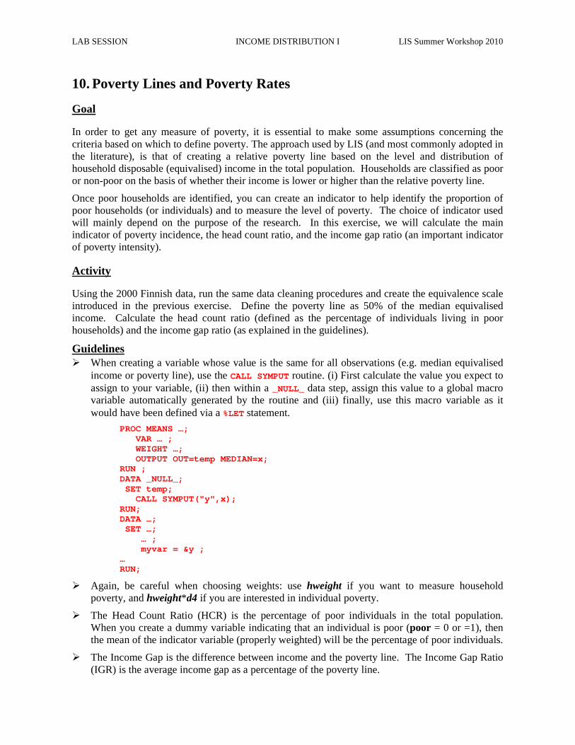
Guidelines � When creating a variable whose value is the same for all observations (e.g. median equivalised
income or poverty line), use the CALL SYMPUT routine. (i) First calculate the value you expect to assign to your variable, (ii) then within a _NULL_ data step, assign this value to a global macro variable automatically generated by the routine and (iii) finally, use this macro variable as it would have been defined via a %LET statement.
PROC MEANS …; VAR … ; WEIGHT …; OUTPUT OUT=temp MEDIAN= x ; RUN ; DATA _NULL_; SET temp; CALL SYMPUT("y", x ); RUN; DATA …; SET …; … ; myvar = &y ; … RUN;
� Again, be careful when choosing weights: use hweight if you want to measure household poverty, and hweight*d4 if you are interested in individual poverty.
� The Head Count Ratio (HCR) is the percentage of poor individuals in the total population. When you create a dummy variable indicating that an individual is poor (poor = 0 or =1), then the mean of the indicator variable (properly weighted) will be the percentage of poor individuals.
� The Income Gap is the difference between income and the poverty line. The Income Gap Ratio (IGR) is the average income gap as a percentage of the poverty line.

� To compute the number of households considered poor in the population, use the option SUMWGT of the PROC MEANS statement.
LAB SESSION INCOME DISTRIBUTION I LIS Summer Workshop 2010
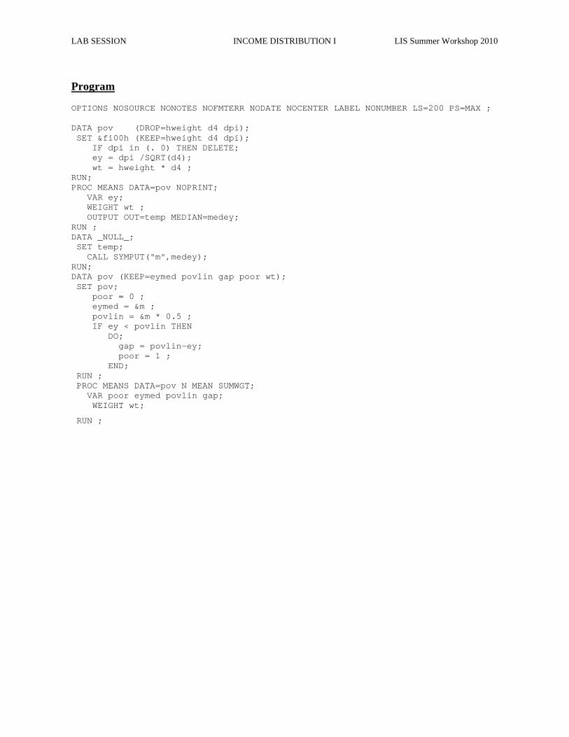
Program
OPTIONS NOSOURCE NONOTES NOFMTERR NODATE NOCENTER LABEL NONUMBER LS=200 PS=MAX ; DATA pov (DROP=hweight d4 dpi); SET &fi00h (KEEP=hweight d4 dpi); IF dpi in (. 0) THEN DELETE; ey = dpi /SQRT(d4); wt = hweight * d4 ; RUN; PROC MEANS DATA=pov NOPRINT; VAR ey; WEIGHT wt ; OUTPUT OUT=temp MEDIAN=medey; RUN ; DATA _NULL_; SET temp; CALL SYMPUT("m",medey); RUN; DATA pov (KEEP=eymed povlin gap poor wt); SET pov; poor = 0 ; eymed = &m ; povlin = &m * 0.5 ; IF ey < povlin THEN DO; gap = povlin-ey; poor = 1 ; END; RUN ; PROC MEANS DATA=pov N MEAN SUMWGT; VAR poor eymed povlin gap; WEIGHT wt;
RUN ;
Results
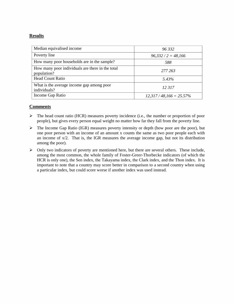
Median equivalised income 96 332 Poverty line 96,332 / 2 = 48,166 How many poor households are in the sample? 588 How many poor individuals are there in the total population?
277 263
Head Count Ratio 5.43% What is the average income gap among poor individuals?
12 317
Income Gap Ratio 12,317 / 48,166 = 25.57%
Comments
� The head count ratio (HCR) measures poverty incidence (i.e., the number or proportion of poor people), but gives every person equal weight no matter how far they fall from the poverty line.
� The Income Gap Ratio (IGR) measures poverty intensity or depth (how poor are the poor), but one poor person with an income of an amount x counts the same as two poor people each with an income of x/2. That is, the IGR measures the average income gap, but not its distribution among the poor).
� Only two indicators of poverty are mentioned here, but there are several others. These include, among the most common, the whole family of Foster-Greer-Thorbecke indicators (of which the HCR is only one), the Sen index, the Takayama index, the Clark index, and the Thon index. It is important to note that a country may score better in comparison to a second country when using a particular index, but could score worse if another index was used instead.
LAB SESSION INCOME DISTRIBUTION I LIS Summer Workshop 2010
11. Elderly and Child Poverty Rates
Goal
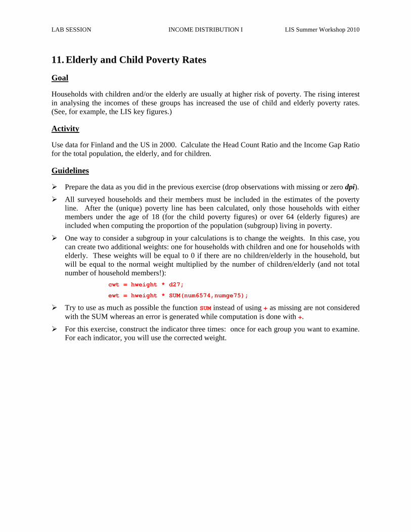
Households with children and/or the elderly are usually at higher risk of poverty. The rising interest in analysing the incomes of these groups has increased the use of child and elderly poverty rates. (See, for example, the LIS key figures.)
Activity
Use data for Finland and the US in 2000. Calculate the Head Count Ratio and the Income Gap Ratio for the total population, the elderly, and for children.
Guidelines
� Prepare the data as you did in the previous exercise (drop observations with missing or zero dpi).
� All surveyed households and their members must be included in the estimates of the poverty line. After the (unique) poverty line has been calculated, only those households with either members under the age of 18 (for the child poverty figures) or over 64 (elderly figures) are included when computing the proportion of the population (subgroup) living in poverty.
� One way to consider a subgroup in your calculations is to change the weights. In this case, you can create two additional weights: one for households with children and one for households with elderly. These weights will be equal to 0 if there are no children/elderly in the household, but will be equal to the normal weight multiplied by the number of children/elderly (and not total number of household members!):
cwt = hweight * d27;
ewt = hweight * SUM(num6574,numge75);
� Try to use as much as possible the function SUM instead of using + as missing are not considered with the SUM whereas an error is generated while computation is done with +.
� For this exercise, construct the indicator three times: once for each group you want to examine. For each indicator, you will use the corrected weight.
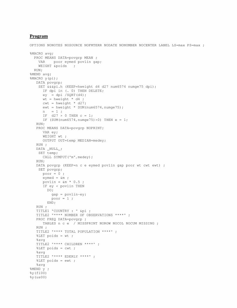
Program
OPTIONS NONOTES NOSOURCE NOFMTERR NODATE NONUMBER NOCENTER LABEL LS=max PS=max ; %MACRO avg; PROC MEANS DATA=povgrp MEAN ; VAR poor eymed povlin gap; WEIGHT &poids ; RUN; %MEND avg; %MACRO y(pi); DATA povgrp; SET &&&pi.h (KEEP=hweight d4 d27 num6574 numge7 5 dpi); IF dpi in (. 0) THEN DELETE; ey = dpi /SQRT(d4); wt = hweight * d4 ; cwt = hweight * d27; ewt = hweight * SUM(num6574,numge75); n = 1 ; IF d27 > 0 THEN c = 1; IF (SUM(num6574,numge75)>0) THEN e = 1; RUN; PROC MEANS DATA=povgrp NOPRINT; VAR ey; WEIGHT wt ; OUTPUT OUT=temp MEDIAN=medey; RUN ; DATA _NULL_; SET temp; CALL SYMPUT("m",medey); RUN; DATA povgrp (KEEP=n c e eymed povlin gap poor wt cwt ewt) ; SET povgrp; poor = 0 ; eymed = &m ; povlin = &m * 0.5 ; IF ey < povlin THEN DO; gap = povlin-ey; poor = 1 ; END; RUN ; TITLE1 "COUNTRY : " &pi ; TITLE2 "**** NUMBER OF OBSERVATIONS ****" ; PROC FREQ DATA=povgrp ; TABLES n c e / MISSPRINT NOROW NOCOL NOCUM M ISSING ; RUN ; TITLE2 "**** TOTAL POPULATION ****" ; %LET poids = wt ; %avg TITLE2 "**** CHILDREN ****" ; %LET poids = cwt ; %avg TITLE2 "**** EDERLY ****" ; %LET poids = ewt ; %avg %MEND y ; %y(fi00) %y(us00)
LAB SESSION INCOME DISTRIBUTION I LIS Summer Workshop 2010
Results
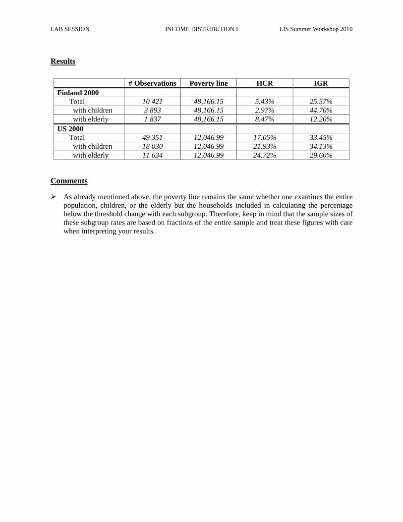
# Observations Poverty line HCR IGR
Finland 2000 Total 10 421 48,166.15 5.43% 25.57% with children 3 893 48,166.15 2.97% 44.70% with elderly 1 837 48,166.15 8.47% 12.20% US 2000 Total 49 351 12,046.99 17.05% 33.45% with children 18 030 12,046.99 21.93% 34.13% with elderly 11 634 12,046.99 24.72% 29.60%
Comments
� As already mentioned above, the poverty line remains the same whether one examines the entire population, children, or the elderly but the households included in calculating the percentage below the threshold change with each subgroup. Therefore, keep in mind that the sample sizes of these subgroup rates are based on fractions of the entire sample and treat these figures with care when interpreting your results.

INCOME DISTRIBUTION II
Ex. 12: Dealing with Extreme Values: Trimming & Bottom- /Top-coding
Ex. 13: Inequality: the Gini Index
Ex. 14: Sensitivity Analysis Using Different Concepts of Income
Ex. 15: Sensitivity Analysis Using Different Equivalence Scales

LAB SESSION INCOME DISTRIBUTION II LIS Summer Workshop 2010
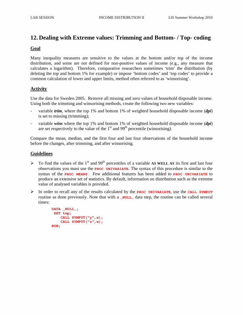
12. Dealing with Extreme values: Trimming and Bottom- / Top- coding
Goal
Many inequality measures are sensitive to the values at the bottom and/or top of the income distribution, and some are not defined for non-positive values of income (e.g., any measure that calculates a logarithm). Therefore, comparative researchers sometimes ‘trim’ the distribution (by deleting the top and bottom 1% for example) or impose ‘bottom codes’ and ‘top codes’ to provide a common calculation of lower and upper limits, method often referred to as ‘winsorising’.
Activity
Use the data for Sweden 2005. Remove all missing and zero values of household disposable income. Using both the trimming and winsorising methods, create the following two new variables:
- variable trim, where the top 1% and bottom 1% of weighted household disposable income (dpi) is set to missing (trimming);
- variable wins where the top 1% and bottom 1% of weighted household disposable income (dpi) are set respectively to the value of the 1st and 99th percentile (winsorising).
Compare the mean, median, and the first four and last four observations of the household income before the changes, after trimming, and after winsorising.
Guidelines
� To find the values of the 1st and 99th percentiles of a variable AS WELL AS its first and last four observations you must use the PROC UNIVARIATE. The syntax of this procedure is similar to the syntax of the PROC MEANS. Few additional features has been added to PROC UNIVARIATE to produce an extensive set of statistics. By default, information on distribution such as the extreme value of analysed variables is provided.
� In order to recall any of the results calculated by the PROC UNIVARIATE, use the CALL SYMPUT routine as done previously. Note that with a _NULL_ data step, the routine can be called several times:
DATA _NULL_; SET tmp; CALL SYMPUT("y",x); CALL SYMPUT("z",w); RUN;
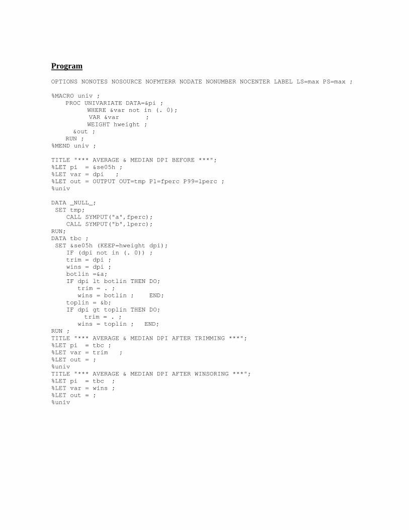
Program
OPTIONS NONOTES NOSOURCE NOFMTERR NODATE NONUMBER NOCENTER LABEL LS=max PS=max ; %MACRO univ ; PROC UNIVARIATE DATA=&pi ; WHERE &var not in (. 0); VAR &var ; WEIGHT hweight ; &out ; RUN ; %MEND univ ; TITLE "*** AVERAGE & MEDIAN DPI BEFORE ***"; %LET pi = &se05h ; %LET var = dpi ; %LET out = OUTPUT OUT=tmp P1=fperc P99=lperc ; %univ DATA _NULL_; SET tmp; CALL SYMPUT("a",fperc); CALL SYMPUT("b",lperc); RUN; DATA tbc ; SET &se05h (KEEP=hweight dpi); IF (dpi not in (. 0)) ; trim = dpi ; wins = dpi ; botlin =&a; IF dpi lt botlin THEN DO; trim = . ; wins = botlin ; END; toplin = &b; IF dpi gt toplin THEN DO; trim = . ; wins = toplin ; END; RUN ; TITLE "*** AVERAGE & MEDIAN DPI AFTER TRIMMING ***" ; %LET pi = tbc ; %LET var = trim ; %LET out = ; %univ TITLE "*** AVERAGE & MEDIAN DPI AFTER WINSORING *** "; %LET pi = tbc ; %LET var = wins ; %LET out = ; %univ
LAB SESSION INCOME DISTRIBUTION II LIS Summer Workshop 2010
Results
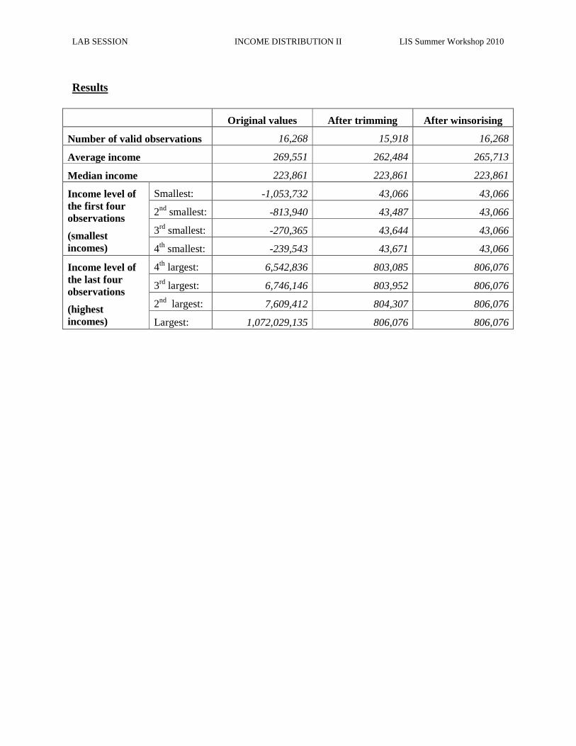
Original values After trimming After winsorising
Number of valid observations 16,268 15,918 16,268
Average income 269,551 262,484 265,713
Median income 223,861 223,861 223,861
Income level of the first four observations
(smallest incomes)
Smallest: -1,053,732 43,066 43,066
2nd smallest: -813,940 43,487 43,066
3rd smallest: -270,365 43,644 43,066
4th smallest: -239,543 43,671 43,066
Income level of the last four observations
(highest incomes)
4th largest: 6,542,836 803,085 806,076
3rd largest: 6,746,146 803,952 806,076
2nd largest: 7,609,412 804,307 806,076
Largest: 1,072,029,135 806,076 806,076

LAB SESSION INCOME DISTRIBUTION II LIS Summer Workshop 2010
13. Inequality: the Gini Index
Goal
This exercise introduces the Gini index, which is one of the most commonly used income inequality indicators.
Activity
Calculate the Gini index on total disposable income for Finland and the US in 2000, after bottom-coding disposable income at 1 percent of its equivalised mean and top-coding at 10 times the unequivalised median.
Guidelines
� Prepare the data as you did in the previous exercise (drop observations with missing or zero dpi).
� In the previous exercise you have seen two different methods of dealing with extreme values, trimming and winsorising (or bottom-/top-coding). The LIS key figures are calculated using a particular type of bottom-/top-coding, which we will replicate in this exercise. The bottom-coding is carried out after the equivalisation of income (on the equivalised income distribution), while the top-coding is carried out before (on the unequivalised distribution) in the following way:
- at the bottom of the distribution, equivalised income is bottom-coded at 1 percent of its equivalised mean, i.e., all observations for which equivalised income is lower than 1% of the average equivalised income are set to that value.
- at the top of the distribution, income is top-coded at 10 times the unequivalised median, i.e., all observations for which unequivalised income (or dpi) is higher than 10 times the median unequivalised income are set to that value.
- Use the same frame as the one created in the previous exercise and adapts it to comply with the LIS definition.
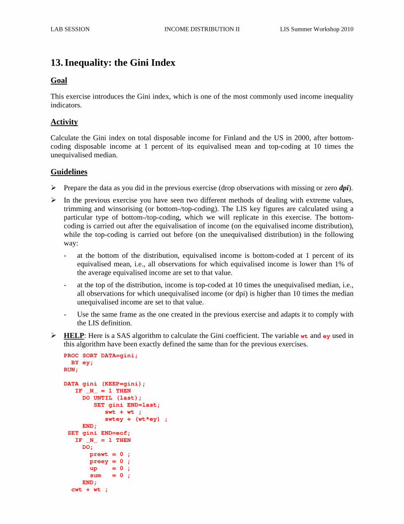
� HELP : Here is a SAS algorithm to calculate the Gini coefficient. The variable wt and ey used in this algorithm have been exactly defined the same than for the previous exercises.
PROC SORT DATA=gini; BY ey; RUN; DATA gini (KEEP=gini); IF _N_ = 1 THEN DO UNTIL (last); SET gini END=last; swt + wt ; swtey + (wt*ey) ; END; SET gini END=eof; IF _N_ = 1 THEN DO; prewt = 0 ; preey = 0 ; up = 0 ; sum = 0 ; END; cwt + wt ;
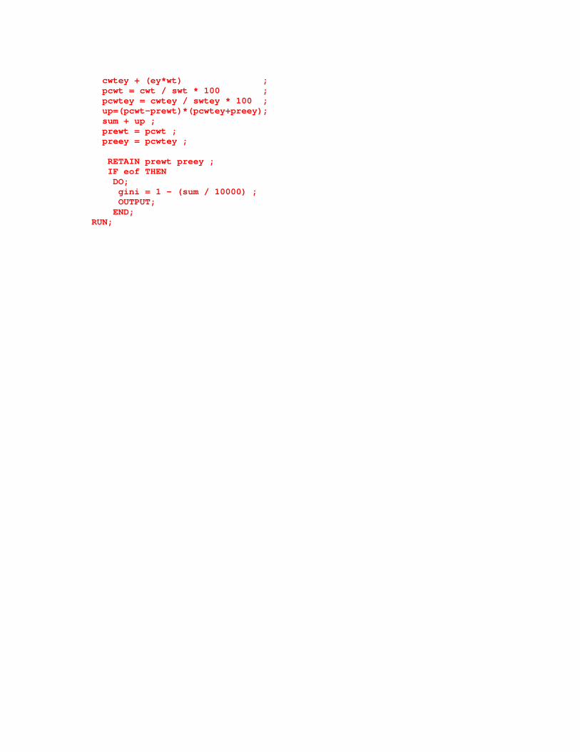
cwtey + (ey*wt) ; pcwt = cwt / swt * 100 ; pcwtey = cwtey / swtey * 100 ; up=(pcwt-prewt)*(pcwtey+preey); sum + up ; prewt = pcwt ; preey = pcwtey ; RETAIN prewt preey ; IF eof THEN DO; gini = 1 - (sum / 10000) ; OUTPUT; END; RUN;
LAB SESSION INCOME DISTRIBUTION II LIS Summer Workshop 2010
Program
OPTIONS NOSOURCE NONOTES NOFMTERR NODATE NOCENTER LABEL NONUMBER LS=MAX PS=MAX ; %MACRO prep ; DATA prep (DROP=hweight); SET &&&pi.h (KEEP=hweight d4 dpi); IF dpi in (. 0) THEN DELETE; ey = &var / SQRT(d4); wt = hweight * d4; RUN; PROC UNIVARIATE DATA=prep NOPRINT; VAR ey dpi ; WEIGHT wt ; OUTPUT OUT=temp MEAN=aveey MEDIAN=medey medpi ; RUN ; DATA _NULL_; SET temp; CALL SYMPUT("a",aveey); CALL SYMPUT("m",medpi); RUN; DATA prep (DROP= botlin toplin); SET prep ; botlin = 0.01 * &a; IF ey < botlin THEN ey = botlin ; toplin = 10 * &m; IF &var > toplin THEN ey = (toplin/(SQRT(d4))) ; RUN ; PROC SORT DATA=prep; BY ey ; RUN ; %MEND prep; %MACRO Gini ; DATA Gini (KEEP=gini) ; IF _N_ = 1 THEN DO UNTIL (last) ; SET prep END=last; swt + wt ; swtey + (wt*ey) ; END ; SET prep END=eof; IF _N_ = 1 THEN DO ; prewt = 0 ; preey = 0 ; up = 0 ; sum = 0 ; END ; cwt + wt ; cwtey + (ey*wt); pcwt = cwt / swt * 100; pcwtey = cwtey / swtey * 100; up = (pcwt-prewt) * (pcwtey+preey) ; sum + up ; prewt = pcwt ; preey = pcwtey ; RETAIN prewt preey ; IF eof THEN DO ; gini=1-(sum / 10000) ;
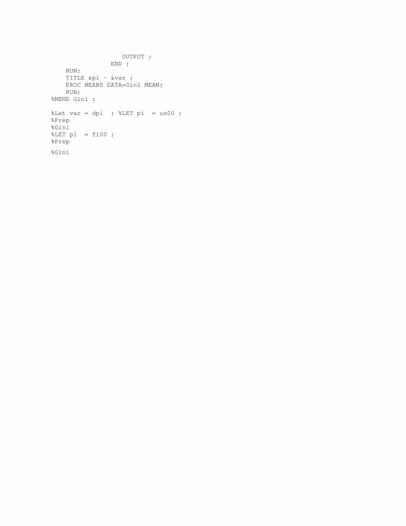
OUTPUT ; END ; RUN; TITLE &pi - &var ; PROC MEANS DATA=Gini MEAN; RUN; %MEND Gini ; %Let var = dpi ; %LET pi = us00 ; %Prep %Gini %LET pi = fi00 ; %Prep
%Gini
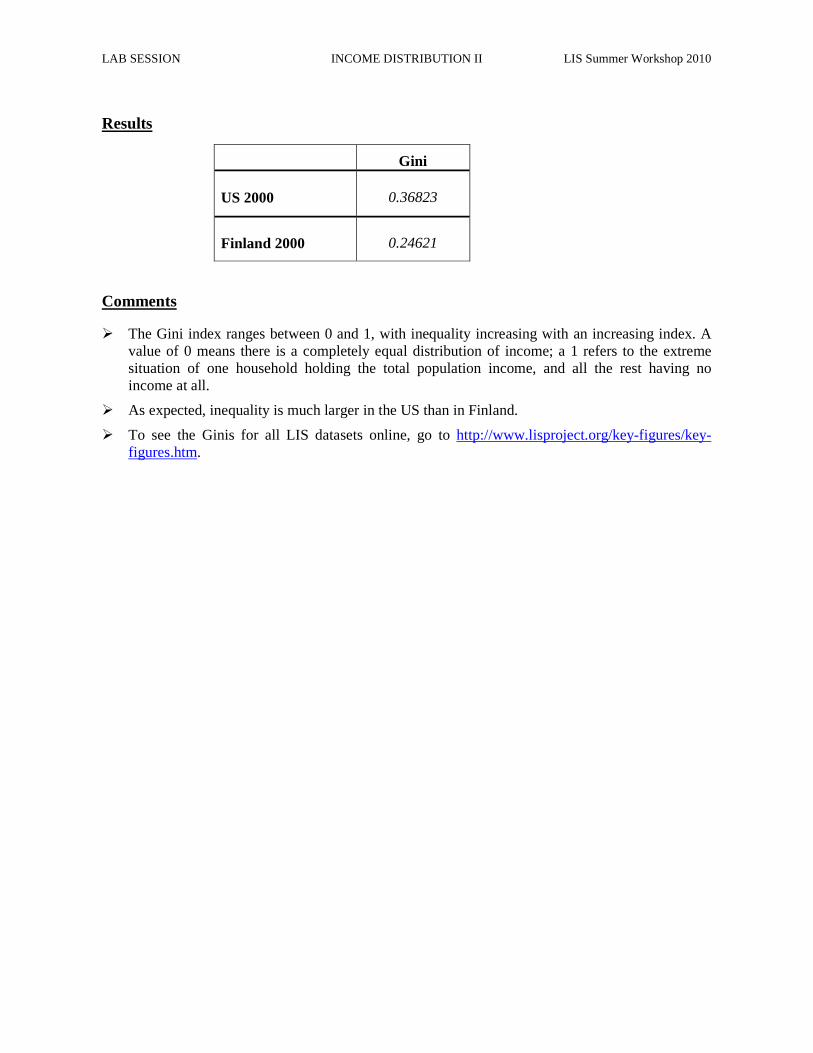
LAB SESSION INCOME DISTRIBUTION II LIS Summer Workshop 2010
Results
Comments
� The Gini index ranges between 0 and 1, with inequality increasing with an increasing index. A value of 0 means there is a completely equal distribution of income; a 1 refers to the extreme situation of one household holding the total population income, and all the rest having no income at all.
� As expected, inequality is much larger in the US than in Finland.
� To see the Ginis for all LIS datasets online, go to http://www.lisproject.org/key-figures/key-figures.htm.
Gini
US 2000 0.36823
Finland 2000 0.24621

LAB SESSION INCOME DISTRIBUTION II LIS Summer Workshop 2010
14. Sensitivity Analysis Using Different Concepts of Income
Goal
When analysing inequality, you should always utilise multiple methods when comparing different countries. Inequality measures can be affected by the indicator used or by the measure of income.
The Gini index may change enormously when it is calculated on income concepts other than disposable income (dpi), which is calculated after transfers and taxes. Instead, you may want to look at market income (mi), which is calculated before taxes and transfers. By computing a Gini index on both income concepts, you can analyse the effect of government influence on the income distribution.
Activity
Calculate the Gini index for Finland and the US in 2000 for both market income and total disposable income, after bottom and top coding as in the previous exercise.
Guidelines
� Prepare the data as you did in the previous exercise. Be careful when choosing your sample. For each of the two income concepts, there will be a different sample of “valid” values (i.e., not missing and not zero). Since we are comparing the two final measures, we want to use the same sample in the two cases. In this exercise, use the sample that drops observations for which dpi is zero or missing. In this case, observations with zero mi but “valid” dpi are kept.
� In this exercise, you will need to create two measures of income: an equivalised disposable income (dpi) as well as an equivalised market income (mi).
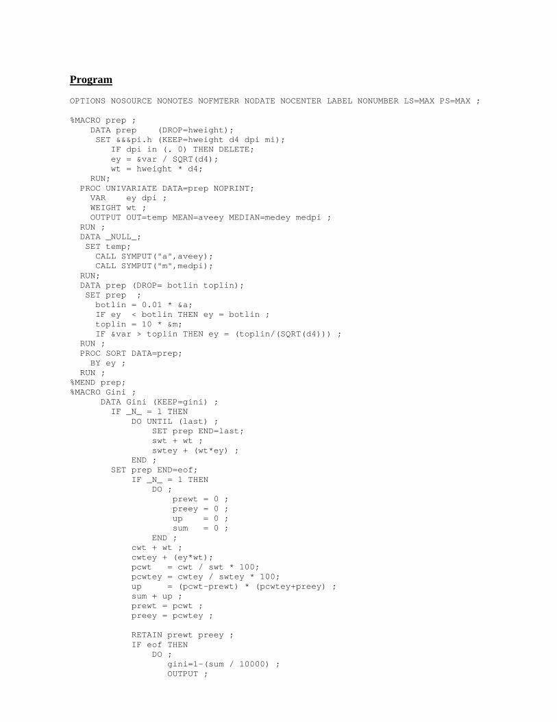
Program
OPTIONS NOSOURCE NONOTES NOFMTERR NODATE NOCENTER LABEL NONUMBER LS=MAX PS=MAX ; %MACRO prep ; DATA prep (DROP=hweight); SET &&&pi.h (KEEP=hweight d4 dpi mi); IF dpi in (. 0) THEN DELETE; ey = &var / SQRT(d4); wt = hweight * d4; RUN; PROC UNIVARIATE DATA=prep NOPRINT; VAR ey dpi ; WEIGHT wt ; OUTPUT OUT=temp MEAN=aveey MEDIAN=medey medpi ; RUN ; DATA _NULL_; SET temp; CALL SYMPUT("a",aveey); CALL SYMPUT("m",medpi); RUN; DATA prep (DROP= botlin toplin); SET prep ; botlin = 0.01 * &a; IF ey < botlin THEN ey = botlin ; toplin = 10 * &m; IF &var > toplin THEN ey = (toplin/(SQRT(d4))) ; RUN ; PROC SORT DATA=prep; BY ey ; RUN ; %MEND prep; %MACRO Gini ; DATA Gini (KEEP=gini) ; IF _N_ = 1 THEN DO UNTIL (last) ; SET prep END=last; swt + wt ; swtey + (wt*ey) ; END ; SET prep END=eof; IF _N_ = 1 THEN DO ; prewt = 0 ; preey = 0 ; up = 0 ; sum = 0 ; END ; cwt + wt ; cwtey + (ey*wt); pcwt = cwt / swt * 100; pcwtey = cwtey / swtey * 100; up = (pcwt-prewt) * (pcwtey+preey) ; sum + up ; prewt = pcwt ; preey = pcwtey ; RETAIN prewt preey ; IF eof THEN DO ; gini=1-(sum / 10000) ; OUTPUT ;
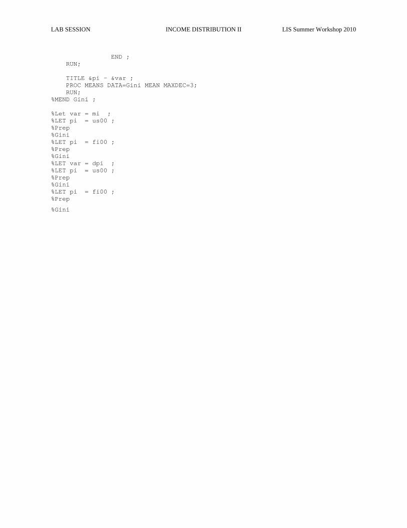
LAB SESSION INCOME DISTRIBUTION II LIS Summer Workshop 2010
END ; RUN; TITLE &pi - &var ; PROC MEANS DATA=Gini MEAN MAXDEC=3; RUN; %MEND Gini ; %Let var = mi ; %LET pi = us00 ; %Prep %Gini %LET pi = fi00 ; %Prep %Gini %LET var = dpi ; %LET pi = us00 ; %Prep %Gini %LET pi = fi00 ; %Prep
%Gini
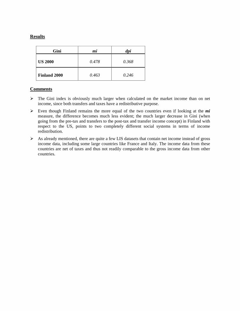
Results
Comments
� The Gini index is obviously much larger when calculated on the market income than on net income, since both transfers and taxes have a redistributive purpose.
� Even though Finland remains the more equal of the two countries even if looking at the mi measure, the difference becomes much less evident; the much larger decrease in Gini (when going from the pre-tax and transfers to the post-tax and transfer income concept) in Finland with respect to the US, points to two completely different social systems in terms of income redistribution.
� As already mentioned, there are quite a few LIS datasets that contain net income instead of gross income data, including some large countries like France and Italy. The income data from these countries are net of taxes and thus not readily comparable to the gross income data from other countries.
Gini mi dpi
US 2000 0.478 0.368
Finland 2000 0.463 0.246
LAB SESSION INCOME DISTRIBUTION II LIS Summer Workshop 2010
15. Sensitivity Analysis Using Different Equivalence Scales
Goal
The LIS equivalence scale (square root of the number of household members) is just one among many possible equivalence scales. Obviously, the choice of the scale will have an impact on the measure calculated. The difference is all the more important when you are considering specific subgroups of the population that are treated differently by the different equivalence scales. In this exercise we will see how the head count ratio (HCR) changes when using the OECD equivalence scales (modified and original) with respect to the LIS equivalence scale.
Activity
Calculate the head count ratio (HCR) for the total population, the child population, and the elderly population in Finland in 2000. Use the LIS equivalence scale, the OECD modified scale, and the OECD original scale to calculate three different measures of equivalised income.
Guidelines
� This exercise utilizes three different equivalence scales:
- LIS scale = square root of the number of persons;
- OECD modified scale = 1 + 0.5*number of other adult members + 0.3 * number of children below 14;
- OECD original scale = 1 + 0.7*number of other adult members + 0.5 * number of children below 14.
� To calculate the head count ratio with the three equivalence scales for the three population groups:
- Calculate three different equivalised incomes:
%LET scale = dpi/SQRT(d4);
%LET scale = dpi/(1 + 0.5*(d4-1-d29) + 0.3*d29);
%LET scale = dpi/(1 + 0.7*(d4-1-d29) + 0.5*d29);
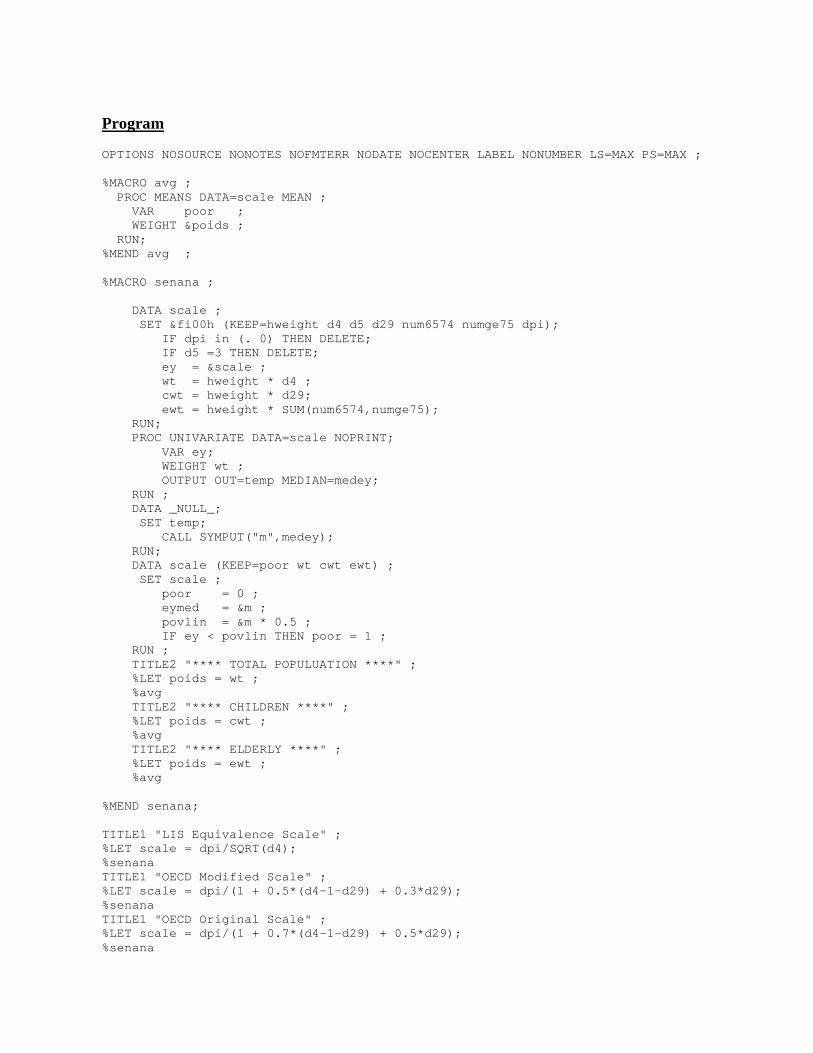
Program
OPTIONS NOSOURCE NONOTES NOFMTERR NODATE NOCENTER LABEL NONUMBER LS=MAX PS=MAX ; %MACRO avg ; PROC MEANS DATA=scale MEAN ; VAR poor ; WEIGHT &poids ; RUN; %MEND avg ; %MACRO senana ; DATA scale ; SET &fi00h (KEEP=hweight d4 d5 d29 num6574 num ge75 dpi); IF dpi in (. 0) THEN DELETE; IF d5 =3 THEN DELETE; ey = &scale ; wt = hweight * d4 ; cwt = hweight * d29; ewt = hweight * SUM(num6574,numge75); RUN; PROC UNIVARIATE DATA=scale NOPRINT; VAR ey; WEIGHT wt ; OUTPUT OUT=temp MEDIAN=medey; RUN ; DATA _NULL_; SET temp; CALL SYMPUT("m",medey); RUN; DATA scale (KEEP=poor wt cwt ewt) ; SET scale ; poor = 0 ; eymed = &m ; povlin = &m * 0.5 ; IF ey < povlin THEN poor = 1 ; RUN ; TITLE2 "**** TOTAL POPULUATION ****" ; %LET poids = wt ; %avg TITLE2 "**** CHILDREN ****" ; %LET poids = cwt ; %avg TITLE2 "**** ELDERLY ****" ; %LET poids = ewt ; %avg %MEND senana; TITLE1 "LIS Equivalence Scale" ; %LET scale = dpi/SQRT(d4); %senana TITLE1 "OECD Modified Scale" ; %LET scale = dpi/(1 + 0.5*(d4-1-d29) + 0.3*d29); %senana TITLE1 "OECD Original Scale" ; %LET scale = dpi/(1 + 0.7*(d4-1-d29) + 0.5*d29); %senana
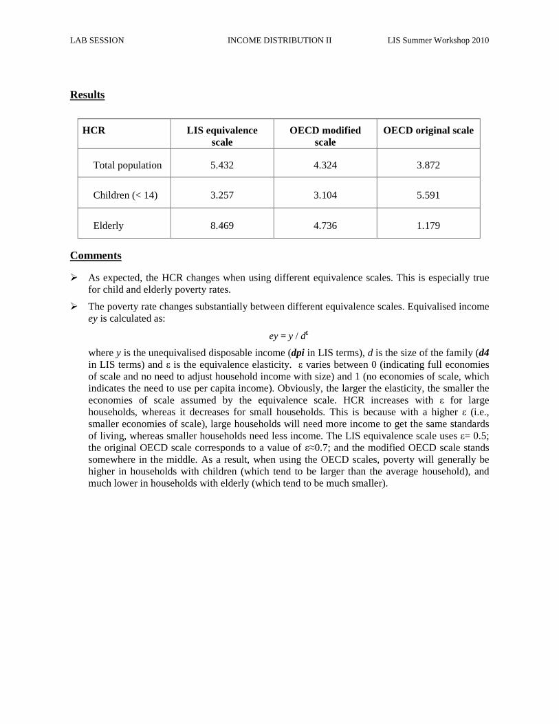
LAB SESSION INCOME DISTRIBUTION II LIS Summer Workshop 2010
Results
HCR LIS equivalence scale
OECD modified scale
OECD original scale
Total population 5.432 4.324 3.872
Children (< 14) 3.257 3.104 5.591
Elderly 8.469 4.736 1.179
Comments
� As expected, the HCR changes when using different equivalence scales. This is especially true for child and elderly poverty rates.
� The poverty rate changes substantially between different equivalence scales. Equivalised income ey is calculated as:
ey = y / dε
where y is the unequivalised disposable income (dpi in LIS terms), d is the size of the family (d4 in LIS terms) and ε is the equivalence elasticity. ε varies between 0 (indicating full economies of scale and no need to adjust household income with size) and 1 (no economies of scale, which indicates the need to use per capita income). Obviously, the larger the elasticity, the smaller the economies of scale assumed by the equivalence scale. HCR increases with ε for large households, whereas it decreases for small households. This is because with a higher ε (i.e., smaller economies of scale), large households will need more income to get the same standards of living, whereas smaller households need less income. The LIS equivalence scale uses ε= 0.5; the original OECD scale corresponds to a value of ε≈0.7; and the modified OECD scale stands somewhere in the middle. As a result, when using the OECD scales, poverty will generally be higher in households with children (which tend to be larger than the average household), and much lower in households with elderly (which tend to be much smaller).


LABOUR MARKET
Ex. 16: Calculating Employment Rates
Ex. 17: Calculating Unemployment Rates
Ex. 18: Person- and Job-specific Characteristics of Employment

LAB SESSION LABOUR MARKET LIS Summer Workshop 2010
16. Calculating Employment Rates
Goal
The employed population can be defined differently depending on the research purpose. In labour market analysis, you may wish to calculate employment rates or run wage regressions. In this case, you may want to identify persons working at a certain moment in time. Within the framework of this strict reference period, a person may be considered as employed as soon as he/she has carried out any work (i.e., the International Labour Organisation (ILO) definition of employment, LIS variable pclfs). Those more interested in the primary employment status at a certain moment in time should not use the ILO definition, but rather look at those whose main activity is employment (LIS variable pcmas).
Those wishing to perform income distribution analyses according to the activity status of individuals (e.g., calculation of poverty rates for the working poor), may choose to focus on employment over a longer reference period. In this case, you need to be able to identify an individual’s primary activity over the income reference period (which in LIS is normally one year, LIS variable pumas).
In this exercise, we identify the employed population according to these three different concepts of employment.
Activity
Calculate employment rates in the US and Germany in 2000 using the three different employment measures. Use the sample of individuals 18 years of age and older. Recode all of those with unclear employment attachment (coded in 900s) to missing.
Guidelines
� The employment rate is the percentage of employed persons in the adult population, which we define here as 18 years of age or older.
� There are three different LIS variables that coincide with the definitions of employment described above:
- persons carrying out any work at present can be identified using pclfs; - persons for whom work is the main activity at present are in pcmas; - persons who are mainly employed during a longer reference period can be found in pumas.
� By definition, those coded in the 900s may have some employment attachment, but the information is too ambiguous to either define them either as “employed” or “not employed”. These individuals were kept in separate detailed categories to allow users to redefine them based on the specific research project. Always check the country-level documentation to determine how you wish to recode those assigned to the 900 (and 400, in pclfs) category.
� In order to measure employment, create dummy variables for employment status, by recoding the original variables into indicators of dichotomous employment status (yes=1 & no=0).
- The generic syntax for this statement is as shown below. NOTE that here the code is kept as simple as possible. In the long run, try to use this statement more often:
ARRAY emp {*} emp1-emp3;
- Use a loop statement to apply similar code on each array elements at the same time.
DO i = 1 TO 3;
IF (900 <= emp(i) <= 999) THEN emp(i) = 1; END;
- The index i starts with the value 1, is then incremented by the increment value each time. The iterations continue as long as the index i is less than or equal to the stop value (here the dimension of the array). If a negative increment is used, then the rules reverse so that the index i decrements to a lower bound. If you don’t use the BY statement the increment is by default equal to 1.
- Note that the index is stored as a variable in your output dataset. Don’t forget to drop it in your output dataset.
DATA emp (DROP=page pclfs pcmas pumas i);
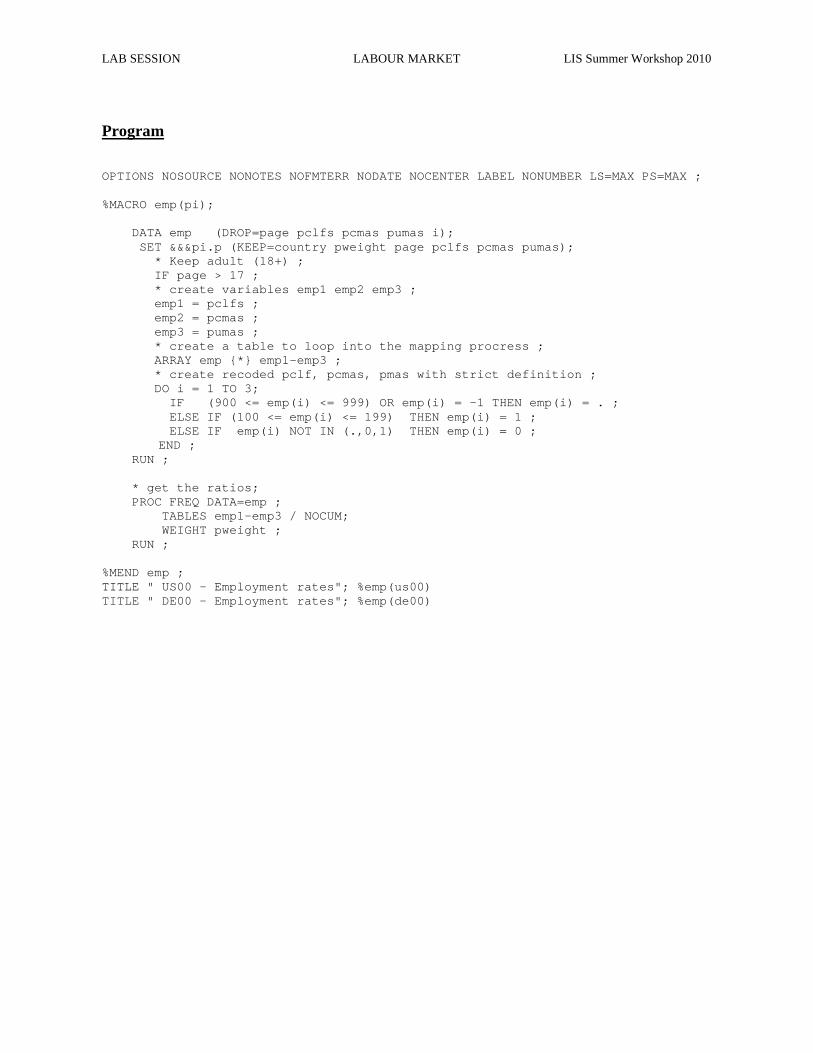
LAB SESSION LABOUR MARKET LIS Summer Workshop 2010
Program
OPTIONS NOSOURCE NONOTES NOFMTERR NODATE NOCENTER LABEL NONUMBER LS=MAX PS=MAX ; %MACRO emp(pi); DATA emp (DROP=page pclfs pcmas pumas i); SET &&&pi.p (KEEP=country pweight page pclfs p cmas pumas); * Keep adult (18+) ; IF page > 17 ; * create variables emp1 emp2 emp3 ; emp1 = pclfs ; emp2 = pcmas ; emp3 = pumas ; * create a table to loop into the mapping pr ocress ; ARRAY emp {*} emp1-emp3 ; * create recoded pclf, pcmas, pmas with stri ct definition ; DO i = 1 TO 3; IF (900 <= emp(i) <= 999) OR emp(i) = -1 THEN emp(i) = . ; ELSE IF (100 <= emp(i) <= 199) THEN emp(i ) = 1 ; ELSE IF emp(i) NOT IN (.,0,1) THEN emp(i ) = 0 ;
END ; RUN ; * get the ratios; PROC FREQ DATA=emp ; TABLES emp1-emp3 / NOCUM; WEIGHT pweight ; RUN ; %MEND emp ; TITLE " US00 - Employment rates"; %emp(us00) TITLE " DE00 - Employment rates"; %emp(de00)
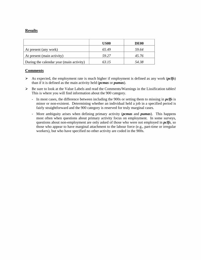
Results
US00 DE00
At present (any work) 65.49 59.64
At present (main activity) 59.27 45.76
During the calendar year (main activity) 63.15 54.38
Comments
� As expected, the employment rate is much higher if employment is defined as any work (pclfs) than if it is defined as the main activity held (pcmas or pumas).
� Be sure to look at the Value Labels and read the Comments/Warnings in the Lissification tables! This is where you will find information about the 900 category.
- In most cases, the difference between including the 900s or setting them to missing in pclfs is minor or non-existent. Determining whether an individual held a job in a specified period is fairly straightforward and the 900 category is reserved for truly marginal cases.
- More ambiguity arises when defining primary activity (pcmas and pumas). This happens most often when questions about primary activity focus on employment. In some surveys, questions about non-employment are only asked of those who were not employed in pclfs, so those who appear to have marginal attachment to the labour force (e.g., part-time or irregular workers), but who have specified no other activity are coded in the 900s.
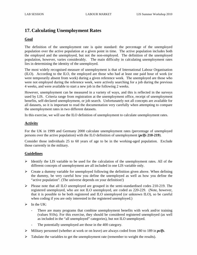
LAB SESSION LABOUR MARKET LIS Summer Workshop 2010
17. Calculating Unemployment Rates
Goal
The definition of the unemployment rate is quite standard: the percentage of the unemployed population over the active population at a given point in time. The active population includes both the employed and the unemployed, but not the non-employed. The definition of the unemployed population, however, varies considerably. The main difficulty in calculating unemployment rates lies in determining the identity of the unemployed.
The most widely recognised measure of unemployment is that of International Labour Organisation (ILO). According to the ILO, the employed are those who had at least one paid hour of work (or were temporarily absent from work) during a given reference week. The unemployed are those who were not employed during the reference week, were actively searching for a job during the previous 4 weeks, and were available to start a new job in the following 2 weeks.
However, unemployment can be measured in a variety of ways, and this is reflected in the surveys used by LIS. Criteria range from registration at the unemployment office, receipt of unemployment benefits, self-declared unemployment, or job search. Unfortunately not all concepts are available for all datasets, so it is important to read the documentation very carefully when attempting to compare the unemployment rates in two different datasets.
In this exercise, we will use the ILO definition of unemployment to calculate unemployment rates.
Activity
For the UK in 1999 and Germany 2000 calculate unemployment rates (percentage of unemployed persons over the active population) with the ILO definition of unemployment (pclfs 210-219).
Consider those individuals 25 to 60 years of age to be in the working-aged population. Exclude those currently in the military.
Guidelines
� Identify the LIS variable to be used for the calculation of the unemployment rates. All of the different concepts of unemployment are all included in one LIS variable only.
� Create a dummy variable for unemployed following the definition given above. When defining the dummy, be very careful how you define the unemployed as well as how you define the “active population”. (The universe depends on your definition!)
� Please note that all ILO unemployed are grouped in the semi-standardised codes 210-219. The registered unemployed, who are not ILO unemployed, are coded as 220-229. (Note, however, that it is possible to be both registered and ILO unemployed (or unknown ILO), so be careful when coding if you are only interested in the registered unemployed.)
� In the UK:
- There are many programs that combine unemployment benefits with work and/or training (values 910s). For this exercise, they should be considered registered unemployed (as well as included in the “all unemployed” categories), but not ILO unemployed.
- The potentially unemployed are those in the 400 category.
� Military personnel (whether at work or on leave) are always coded from 180 to 189 in pclfs.
� Tabulate the variables to get the unemployment rate (remember to weight the results).
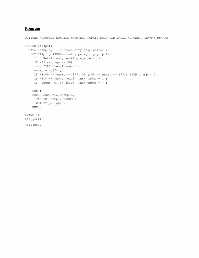
Program OPTIONS NOSOURCE NONOTES NOFMTERR NODATE NOCENTER LABEL NONUMBER LS=MAX PS=MAX;
%MACRO lfc(pi);
DATA unemploy (DROP=country page pclfs) ;
SET &&&pi.p (KEEP=country pweight page pclfs);
*--- Retain only working age persons ;
IF (25 <= page <= 60) ;
*--- "ILO Unemployment" ;
unemp = pclfs ;
IF ((100 <= unemp <= 179) OR (190 <= unemp <= 199)) THEN unemp = 0 ;
IF (210 <= unemp <=219) THEN unemp = 1 ;
IF unemp NOT IN (0,1) THEN unemp = . ;
RUN ;
PROC FREQ DATA=unemploy ;
TABLES unemp / NOCUM ;
WEIGHT pweight ;
RUN ;
%MEND lfc ;
%lfc(uk99)
%lfc(de00)
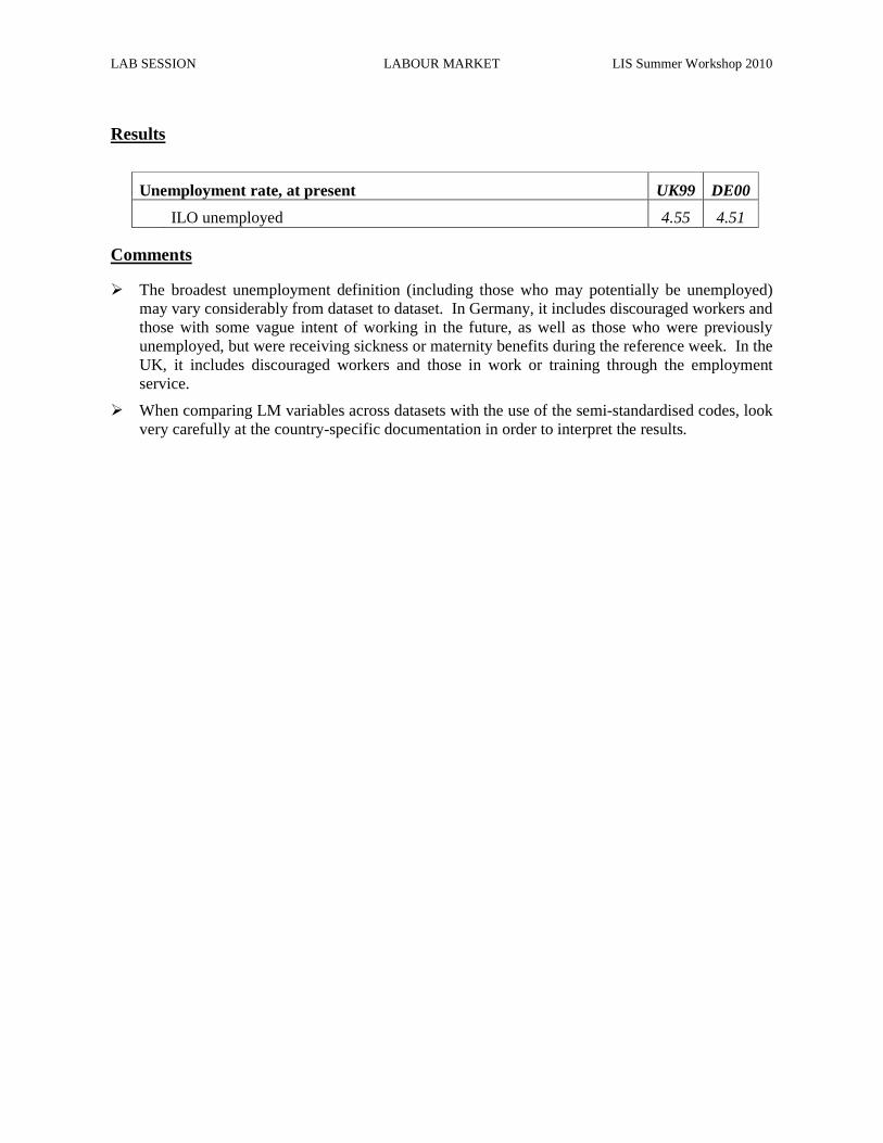
LAB SESSION LABOUR MARKET LIS Summer Workshop 2010
Results
Unemployment rate, at present UK99 DE00
ILO unemployed 4.55 4.51
Comments
� The broadest unemployment definition (including those who may potentially be unemployed) may vary considerably from dataset to dataset. In Germany, it includes discouraged workers and those with some vague intent of working in the future, as well as those who were previously unemployed, but were receiving sickness or maternity benefits during the reference week. In the UK, it includes discouraged workers and those in work or training through the employment service.
� When comparing LM variables across datasets with the use of the semi-standardised codes, look very carefully at the country-specific documentation in order to interpret the results.

LAB SESSION LABOUR MARKET LIS Summer Workshop 2010
18. Person- and Job-specific Characteristics of Employment
Goal
There are a number of employment characteristics that may interest researchers. This exercise introduces you to a few of the person- and job-specific variables that are available from LIS.
Activity
For Spain in 2000, create a SAS dataset containing page, pweight, pclfs, and the following:
- Characteristics of the Individual � continuous: phoursu, pweektl � categorical: psecjob, psearch, pcare
- Characteristics of the Primary Job � categorical: pactiv, pind, ptypewk, pfulpar
This exercise uses a sample of adults (16 and over). From pclfs create a dummy variable (emp) that will be coded 0 for individuals that are not employed and 1 for individuals that are employed. Using the characteristics of the individual (continuous variables phoursu, pweektl as well as the newly created employment dummy variable, emp), find the weighted mean, minimum, and maximum. Repeat the same calculations (for the same variables) after you “clean” the data (see the Guidelines for instructions).
Finally, tabulate the dummy variable (emp) with each categorical variable. Run this tabulation twice: (1) without weights and with those individuals who are coded -1; (2) with weights and excluding those who are coded -1.
Use the information from your output and/or the documentation to answer the following questions:
1. What are the minimum and maximum numbers of usual weekly hours for the employed?
_____________________________________________________________________________
Explain these results.
_____________________________________________________________________________
_____________________________________________________________________________
What are the implications for interpreting the average hours worked reported above?
_____________________________________________________________________________
_____________________________________________________________________________
_____________________________________________________________________________
2. Why does phoursu equal 0 for all observations of those not employed? When is it possible for phoursu to equal to 0 for some of those employed?
_____________________________________________________________________________
_____________________________________________________________________________
_____________________________________________________________________________
3. How is it possible that some of those who are not employed reported 52 weeks of employment?
_____________________________________________________________________________
_____________________________________________________________________________
_____________________________________________________________________________
4. Which variables have no observations equal to -1 among the employed and all observations equal to -1 among those not employed?
_____________________________________________________________________________
What does this tell us about the universe of those variables?
_____________________________________________________________________________
_____________________________________________________________________________
5. Why does ptypewk have some observations equal to -1 among the employed?
_____________________________________________________________________________
_____________________________________________________________________________
_____________________________________________________________________________
6. Which variables have no observations equal to -1 for either group?
_____________________________________________________________________________
What does this tell us about the universe of those variables?
_____________________________________________________________________________
_____________________________________________________________________________
Guidelines
� When creating your employment dummy variable, be sure to include only those you can clearly identify as being either employed or not employed. In other words, be careful what you do with the 900s codes in pclfs.
� The variables phoursu and pweektl (as well as all other time variables), are peculiar in that they may be continuous and discrete at the same time: all the values between 0 and 999 are normal continuous values, representing the duration of time (either hours of weeks), but on top of those there may be some discrete values, notably:
- the value -9 for phoursu and phoursa stands for “hours vary”;
- all the values greater or equal to 1000 indicate partial or incomplete information, where the 1000 is a flag and stands for “at least xx number of hours” (see Section D of the introduction of the Labour Market Variables Guidelines).
As a consequence, none of these values should be used as such (as they do not represent actual numbers of hours / weeks), and they should be excluded from the sample unless recoded to a valid value.
� The syntax of the SAS procedure is standardized. To avoid repeating several times, the same code with different parameters (e.g.: different analytical variable), you can create a generic SAS macro that allows you to only call the relevant parameter each time you invoke the macro. Find
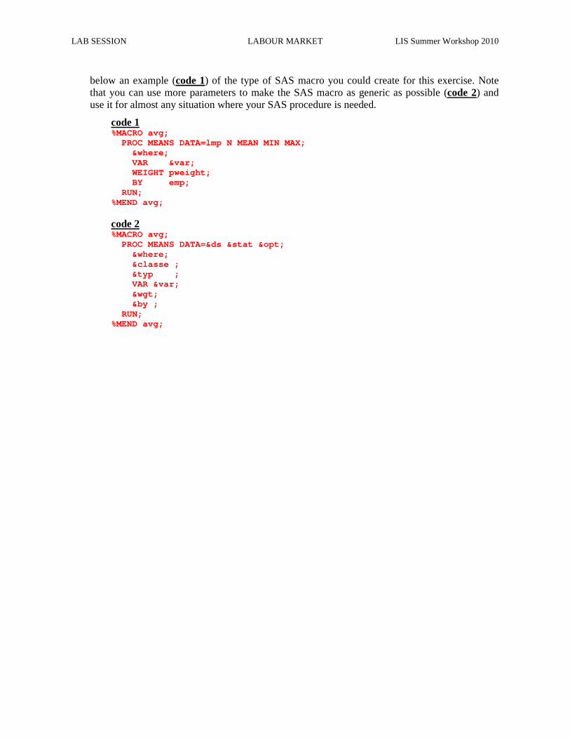
LAB SESSION LABOUR MARKET LIS Summer Workshop 2010
below an example (code 1) of the type of SAS macro you could create for this exercise. Note that you can use more parameters to make the SAS macro as generic as possible (code 2) and use it for almost any situation where your SAS procedure is needed.
code 1 %MACRO avg; PROC MEANS DATA=lmp N MEAN MIN MAX; &where; VAR &var; WEIGHT pweight; BY emp; RUN; %MEND avg;
code 2 %MACRO avg; PROC MEANS DATA=&ds &stat &opt; &where; &classe ; &typ ; VAR &var; &wgt; &by ; RUN; %MEND avg;
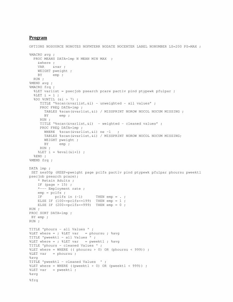
Program
OPTIONS NOSOURCE NONOTES NOFMTERR NODATE NOCENTER LABEL NONUMBER LS=200 PS=MAX ; %MACRO avg ; PROC MEANS DATA=lmp N MEAN MIN MAX ; &where ; VAR &var ; WEIGHT pweight ; BY emp ; RUN ; %MEND avg ; %MACRO frq ; %LET varlist = psecjob psearch pcare pactiv pind ptypewk pfulpar ; %LET i = 1 ; %DO %UNTIL (&i > 7) ; TITLE “%scan(&varlist,&i) - unweighted - all v alues” ; PROC FREQ DATA=lmp ; TABLES %scan(&varlist,&i) / MISSPRINT NOROW NOCOL NOCUM MISSING ; BY emp ; RUN ; TITLE “%scan(&varlist,&i) - weighted - cleane d values” ; PROC FREQ DATA=lmp ; WHERE %scan(&varlist,&i) ne -1 ; TABLES %scan(&varlist,&i) / MISSPRINT NOROW NOCOL NOCUM MISSING; WEIGHT pweight ; BY emp ; RUN ; %LET i = %eval(&i+1) ; %END ; %MEND frq ; DATA lmp ; SET &es00p (KEEP=pweight page pclfs pactiv pind pt ypewk pfulpar phoursu pweektl psecjob psearch pcare); * Retain Adults ; IF (page > 15) ; *--- Employment rate ; emp = pclfs ; IF pclfs in (-1) THEN emp = . ; ELSE IF (100<=pclfs<=199) THEN emp = 1 ; ELSE IF (200<=pclfs<=999) THEN emp = 0 ; RUN ; PROC SORT DATA=lmp ; BY emp ; RUN ; TITLE "phours - all Values " ; %LET where = ; %LET var = phoursu ; %avg TITLE "pweektl - all Values " ; %LET where = ; %LET var = pweektl ; %avg TITLE "phours - cleaned Values " ; %LET where = WHERE (( phoursu > 0) OR (phoursu < 99 9)) ; %LET var = phoursu ; %avg TITLE "pweektl - cleaned Values " ; %LET where = WHERE ((pweektl > 0) OR (pweektl < 999 )) ; %LET var = pweektl ; %avg
%frq
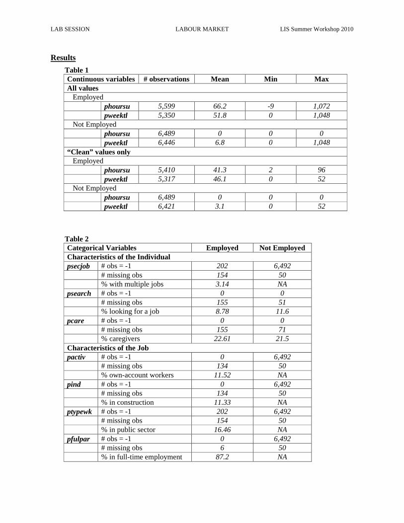
LAB SESSION LABOUR MARKET LIS Summer Workshop 2010
Results
Table 1 Continuous variables # observations Mean Min Max All values Employed phoursu 5,599 66.2 -9 1,072 pweektl 5,350 51.8 0 1,048 Not Employed phoursu 6,489 0 0 0 pweektl 6,446 6.8 0 1,048 “Clean” values only Employed phoursu 5,410 41.3 2 96 pweektl 5,317 46.1 0 52 Not Employed phoursu 6,489 0 0 0 pweektl 6,421 3.1 0 52
Table 2 Categorical Variables Employed Not Employed Characteristics of the Individual psecjob # obs = -1 202 6,492 # missing obs 154 50 % with multiple jobs 3.14 NA psearch # obs = -1 0 0 # missing obs 155 51 % looking for a job 8.78 11.6 pcare # obs = -1 0 0 # missing obs 155 71 % caregivers 22.61 21.5 Characteristics of the Job pactiv # obs = -1 0 6,492 # missing obs 134 50 % own-account workers 11.52 NA pind # obs = -1 0 6,492 # missing obs 134 50 % in construction 11.33 NA ptypewk # obs = -1 202 6,492 # missing obs 154 50 % in public sector 16.46 NA pfulpar # obs = -1 0 6,492 # missing obs 6 50 % in full-time employment 87.2 NA
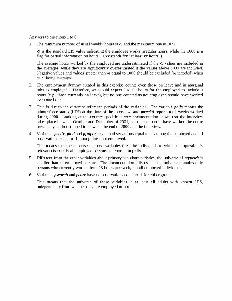
Answers to questions 1 to 6:
1. The minimum number of usual weekly hours is -9 and the maximum one is 1072.
-9 is the standard LIS value indicating the employee works irregular hours, while the 1000 is a flag for partial information on hours (10xx stands for “at least xx hours”).
The average hours worked by the employed are underestimated if the -9 values are included in the averages, while they are significantly overestimated if the values above 1000 are included. Negative values and values greater than or equal to 1000 should be excluded (or recoded) when calculating averages.
2. The employment dummy created in this exercise counts even those on leave and in marginal jobs as employed. Therefore, we would expect “usual” hours for the employed to include 0 hours (e.g., those currently on leave), but no one counted as not employed should have worked even one hour.
3. This is due to the different reference periods of the variables. The variable pclfs reports the labour force status (LFS) at the time of the interview, and pweektl reports total weeks worked during 2000. Looking at the country-specific survey documentation shows that the interview takes place between October and December of 2001, so a person could have worked the entire previous year, but stopped in between the end of 2000 and the interview.
4. Variables pactiv, pind and pfulpar have no observations equal to -1 among the employed and all observations equal to -1 among those not employed.
This means that the universe of those variables (i.e., the individuals to whom this question is relevant) is exactly all employed persons as reported in pclfs.
5. Different from the other variables about primary job characteristics, the universe of ptypewk is smaller than all employed persons. The documentation tells us that the universe contains only persons who currently work at least 15 hours per week, not all employed individuals.
6. Variables psearch and pcare have no observations equal to -1 for either group.
This means that the universe of those variables is at least all adults with known LFS, independently from whether they are employed or not.

STACKED DATA
(OPTION 1)
Ex. 19: A Cross-national Comparison Using Stacked Data

LAB SESSION STACKED DATA LIS Summer Workshop 2010
19. A Cross-national Comparison Using Stacked Data
Goal
In this exercise, we combine household- and person-level files across countries to run a regression estimating the usual hours of the working-aged civilian population, utilizing a number of the techniques learned in earlier exercises. In addition, we show the importance of weighting correctly when combining files with very diverse sample sizes and weighting structures.
Activity
For Ireland and Austria in 2000, do the following:
1. Using the household-level file:
a. Create a sample containing casenum, hweight, d4, d5, and dpi.
b. Create a dummy variable (poorhh) indicating that a household is poor (as defined by having less than 50 percent of median equivalised disposable income).
c. Create a variable (count) containing the number of households in the sample (that is the same for all observations within the country).
d. Create a new weight that normalizes the household weight to 1.
e. Save your file in the temporary LIS directory for later use. (See Guidelines below for details.)
2. Using the person-level file, create a sample of non-military working-aged adults (25 through 60).
a. Include the variables country, casenum, pweight, page, psex, peduc, ptocc, phoursu, pclfs, and pcare.
b. Using pclfs, drop any individuals who are in the military (both regular armed forces and conscripts).
c. Run the LIS include program to recode education. Recode educ to missing if education is not in one of the major classifications (1 to 3).
d. Using pcare, create a dummy variable (ccare) that indicates care of children.
e. Recode phoursu to missing if the usual hours worked vary.
f. Create dummy variables for gender (female) and country (at00).
3. For each country, merge the person- and household-level files keeping only working-age civilian adults in households without missing or zero dpi.
a. Note: Your final file will be at the person level. You should only retain observations that include information from both of the two samples you created above.)
b. Save the merged file with the same temporary file name as you used when saving the household data.
4. Create your final sample by appending all of your country-level merged files.
a. Create a variable that defines each household in your combined sample (i.e., every combination of country and casenum will have a unique value).
b. Save your final combined file to the temporary directory.
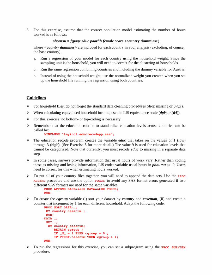
5. For this exercise, assume that the correct population model estimating the number of hours worked is as follows:
phoursu = f(page educ poorhh female ccare <country dummies>)
where <country dummies> are included for each country in your analysis (excluding, of course, the base country).
a. Run a regression of your model for each country using the household weight. Since the sampling unit is the household, you will need to correct for the clustering of households.
b. Run the same regression combining countries and including the dummy variable for Austria.
c. Instead of using the household weight, use the normalized weight you created when you set up the household file running the regression using both countries.
Guidelines
� For household files, do not forget the standard data cleaning procedures (drop missing or 0 dpi).
� When calculating equivalised household income, use the LIS equivalence scale (dpi/sqrt(d4)).
� For this exercise, no bottom- or top-coding is necessary.
� Remember that the education routine to standardize education levels across countries can be called by:
%INCLUDE "&myincl.educrecodepp.sas";
� The education recode program creates the variable educ that takes on the values of 1 (low) through 3 (high). (See Exercise 8 for more detail.) The value 9 is used for education levels that cannot be categorized. Note that currently, you must recode educ to missing in a separate data step.
� In some cases, surveys provide information that usual hours of work vary. Rather than coding these as missing and losing information, LIS codes variable usual hours in phoursu as -9. Users need to correct for this when estimating hours worked.
� To put all of your country files together, you will need to append the data sets. Use the PROC
APPEND procedure and use the option FORCE to avoid any SAS format errors generated if two different SAS formats are used for the same variables.
PROC APPEND BASE=ie00 DATA=at00 FORCE; RUN;
� To create the cgroup variable (i) sort your dataset by country and casenum, (ii) and create a counter that increment by 1 for each different household. Adapt the following code.
PROC SORT DATA=…; BY country casenum ; RUN; DATA …; SET …; BY country casenum; RETAIN cgroup ; IF _N_ = 1 THEN cgroup = 0 ; IF FIRST.casenum THEN cgroup + 1; RUN;
� To run the regressions for this exercise, you can set a subprogram using the PROC SURVGEN procedure.
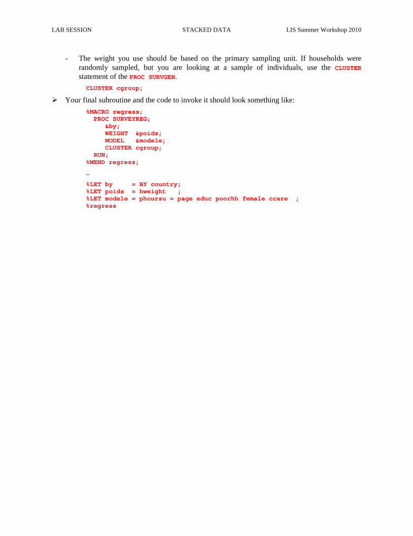
LAB SESSION STACKED DATA LIS Summer Workshop 2010
- The weight you use should be based on the primary sampling unit. If households were randomly sampled, but you are looking at a sample of individuals, use the CLUSTER statement of the PROC SURVGEN.
CLUSTER cgroup;
� Your final subroutine and the code to invoke it should look something like:
%MACRO regress; PROC SURVEYREG; &by; WEIGHT &poids; MODEL &modele; CLUSTER cgroup; RUN; %MEND regress;
…
%LET by = BY country; %LET poids = hweight ; %LET modele = phoursu = page educ poorhh female cca re ; %regress
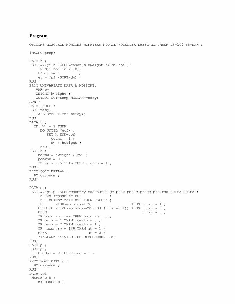
Program
OPTIONS NOSOURCE NONOTES NOFMTERR NODATE NOCENTER LABEL NONUMBER LS=200 PS=MAX ; %MACRO prep; DATA h ; SET &&&pi.h (KEEP=casenum hweight d4 d5 dpi ); IF dpi not in (. 0); IF d5 ne 3 ; ey = dpi /SQRT(d4) ; RUN; PROC UNIVARIATE DATA=h NOPRINT; VAR ey; WEIGHT hweight ; OUTPUT OUT=temp MEDIAN=medey; RUN ; DATA _NULL_; SET temp; CALL SYMPUT("m",medey); RUN; DATA h ; IF _N_ = 1 THEN DO UNTIL (eof) ; SET h END=eof; count + 1 ; sw + hweight ; END ; SET h ; normw = hweight / sw ; poorhh = 0 ; IF ey < 0.5 * &m THEN poorhh = 1 ; RUN ; PROC SORT DATA=h ; BY casenum ; RUN; DATA p ; SET &&&pi.p (KEEP=country casenum page psex peduc ptocc phoursu pclfs pcare); IF (25 <=page <= 60) ; IF (180<=pclfs<=189) THEN DELETE ; IF (100<=pcare<=119) THEN ccare = 1 ; ELSE IF ((120<=pcare<=299) OR (pcare=901)) THEN ccare = 0 ; ELSE ccare = . ; IF phoursu = -9 THEN phoursu = . ; IF psex = 1 THEN female = 0 ; IF psex = 2 THEN female = 1 ; IF country = 139 THEN at = 1 ; ELSE at = 0 ; %INCLUDE "&myincl.educrecodepp.sas"; RUN; DATA p ; SET p ; IF educ = 9 THEN educ = . ; RUN; PROC SORT DATA=p ; BY casenum ; RUN; DATA &pi ; MERGE p h ; BY casenum ;
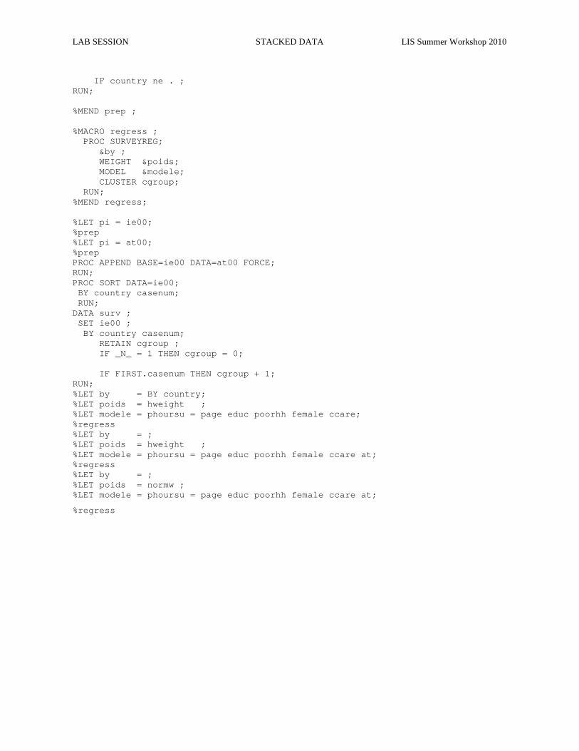
LAB SESSION STACKED DATA LIS Summer Workshop 2010
IF country ne . ; RUN; %MEND prep ; %MACRO regress ; PROC SURVEYREG; &by ; WEIGHT &poids; MODEL &modele; CLUSTER cgroup; RUN; %MEND regress; %LET pi = ie00; %prep %LET pi = at00; %prep PROC APPEND BASE=ie00 DATA=at00 FORCE; RUN; PROC SORT DATA=ie00; BY country casenum; RUN; DATA surv ; SET ie00 ; BY country casenum; RETAIN cgroup ; IF _N_ = 1 THEN cgroup = 0; IF FIRST.casenum THEN cgroup + 1; RUN; %LET by = BY country; %LET poids = hweight ; %LET modele = phoursu = page educ poorhh female cca re; %regress %LET by = ; %LET poids = hweight ; %LET modele = phoursu = page educ poorhh female cca re at; %regress %LET by = ; %LET poids = normw ; %LET modele = phoursu = page educ poorhh female cca re at;
%regress
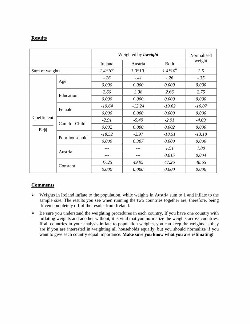
Results
Weighted by hweight Normalised
weight Ireland Austria Both
Sum of weights 1.4*106 3.0*103 1.4*106 2.5
Coefficient _________
P>|t|
Age -.26 -.41 -.26 -.35
0.000 0.000 0.000 0.000
Education 2.66 3.38 2.66 2.75
0.000 0.000 0.000 0.000
Female -19.64 -12.24 -19.62 -16.07
0.000 0.000 0.000 0.000
Care for Child -2.91 -5.49 -2.91 -4.09
0.002 0.000 0.002 0.000
Poor household -18.52 -2.97 -18.51 -13.18
0.000 0.307 0.000 0.000
Austria --- --- 1.51 1.80
--- --- 0.015 0.004
Constant 47.25 49.95 47.26 48.65
0.000 0.000 0.000 0.000
Comments
� Weights in Ireland inflate to the population, while weights in Austria sum to 1 and inflate to the sample size. The results you see when running the two countries together are, therefore, being driven completely off of the results from Ireland.
� Be sure you understand the weighting procedures in each country. If you have one country with inflating weights and another without, it is vital that you normalize the weights across countries. If all countries in your analysis inflate to population weights, you can keep the weights as they are if you are interested in weighting all households equally, but you should normalize if you want to give each country equal importance. Make sure you know what you are estimating!
LWS BASICS
(OPTION 2)
Ex. 20: Differences in Concepts of Net Worth
Ex. 21: Asset Participation

LAB SESSION FINAL EXERCISE LIS Summer Workshop 2010
20. Differences in Concepts of Net Worth
Goal
Estimates of net worth can differ substantially depending on the wealth measure you use. In this exercise, you will begin to familiarize yourself with the summary measures in LWS and determine the differences in portfolio compositions for the whole population using two different definitions of net worth.
Activity
Calculate summary statistics (mean and median) for two LWS net worth concepts, nw1 and nw2, as defined in the LWS Quick Reference Guide. Determine the differences in portfolio compositions for these two measures in Italy and Sweden in 2002.
Guidelines
� Don’t forget to change the project in your job submission panel to LWS.
� Use the LWS Quick Reference Guide to identify the components of nw1 and nw2.
� For the first part of the exercise calculate the means and medians for the two net worth measures.
� For the second part of the exercise calculate the means of the components and take the appropriate ratios to find the shares.
� For business holdings, use the measure for business equity, if available. Otherwise, use business assets. In order to do this, you will need to check the country-specific documentation for the availability of business assets, business debt, and business equity.
� Use the country documentation to check for differences in variable construction.
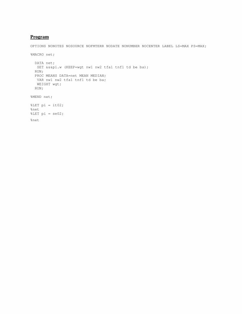
Program
OPTIONS NONOTES NOSOURCE NOFMTERR NODATE NONUMBER NOCENTER LABEL LS=MAX PS=MAX; %MACRO net; DATA net; SET &&&pi.w (KEEP=wgt nw1 nw2 tfa1 tnf1 td be ba ); RUN; PROC MEANS DATA=net MEAN MEDIAN; VAR nw1 nw2 tfa1 tnf1 td be ba; WEIGHT wgt; RUN; %MEND net; %LET pi = it02; %net %LET pi = se02;
%net
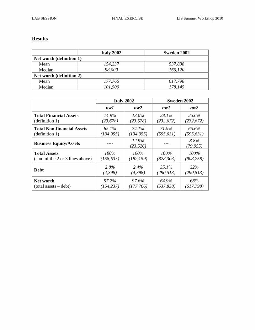
LAB SESSION FINAL EXERCISE LIS Summer Workshop 2010
Results
Italy 2002 Sweden 2002 Net worth (definition 1)
Mean 154,237 537,838 Median 98,000 165,120
Net worth (definition 2) Mean 177,766 617,798 Median 101,500 178,145
Italy 2002 Sweden 2002
nw1 nw2 nw1 nw2
Total Financial Assets (definition 1)
14.9% (23,678)
13.0% (23,678)
28.1% (232,672)
25.6% (232,672)
Total Non-financial Assets (definition 1)
85.1% (134,955)
74.1% (134,955)
71.9% (595,631)
65.6% (595,631)
Business Equity/Assets ---- 12.9%
(23,526) ---
8.8% (79,955)
Total Assets (sum of the 2 or 3 lines above)
100% (158,633)
100% (182,159)
100% (828,303)
100% (908,258)
Debt 2.8%
(4,398) 2.4%
(4,398) 35.1%
(290,513) 32%
(290,513)
Net worth (total assets – debt)
97.2% (154,237)
97.6% (177,766)
64.9% (537,838)
68% (617,798)

LAB SESSION FINAL EXERCISE LIS Summer Workshop 2010
21. Asset Participation
Goal
The goal of this exercise is to become familiar with different types of assets in the LWS data and to compare asset participation of the elderly with the population as a whole.
Activity
Calculate participation in the three assets (deposit accounts, stocks, investment real estate, business assets/equity) for the total population, and the elderly population in Finland in 1998, Italy 2002 and Sweden 2002.
Use the information from your output and/or the documentation to answer the following questions:
1. In which country are households more inclined to have risky portfolios?
_____________________________________________________________________________
_____________________________________________________________________________
_____________________________________________________________________________
2. What happens to deposit accounts as the population ages?
_____________________________________________________________________________
_____________________________________________________________________________
___________________________________________________________________
Guidelines
� Use the LWS Quick Reference Guide to help you with the job submission.
� Identify the wealth variables needed to calculate the participation rates using the documentation to check whether each of these components exists in each of these countries.
� Create dummy variables for each of the wealth components to indicate that a household is holding a particular asset. Here is an example of the dummy generation:
dda = 0 ;
IF ((da > 0 ) OR (da = .)) THEN dda = 1 ;
� For business holdings, use the measure for business equity, if available. Otherwise, use business assets. In order to do this, you will need to check the country-specific documentation for the availability of business assets, business debt, and business equity.
� When measuring assets of the elderly population, define elderly households as those with a head or spouse 65 years of age or older.
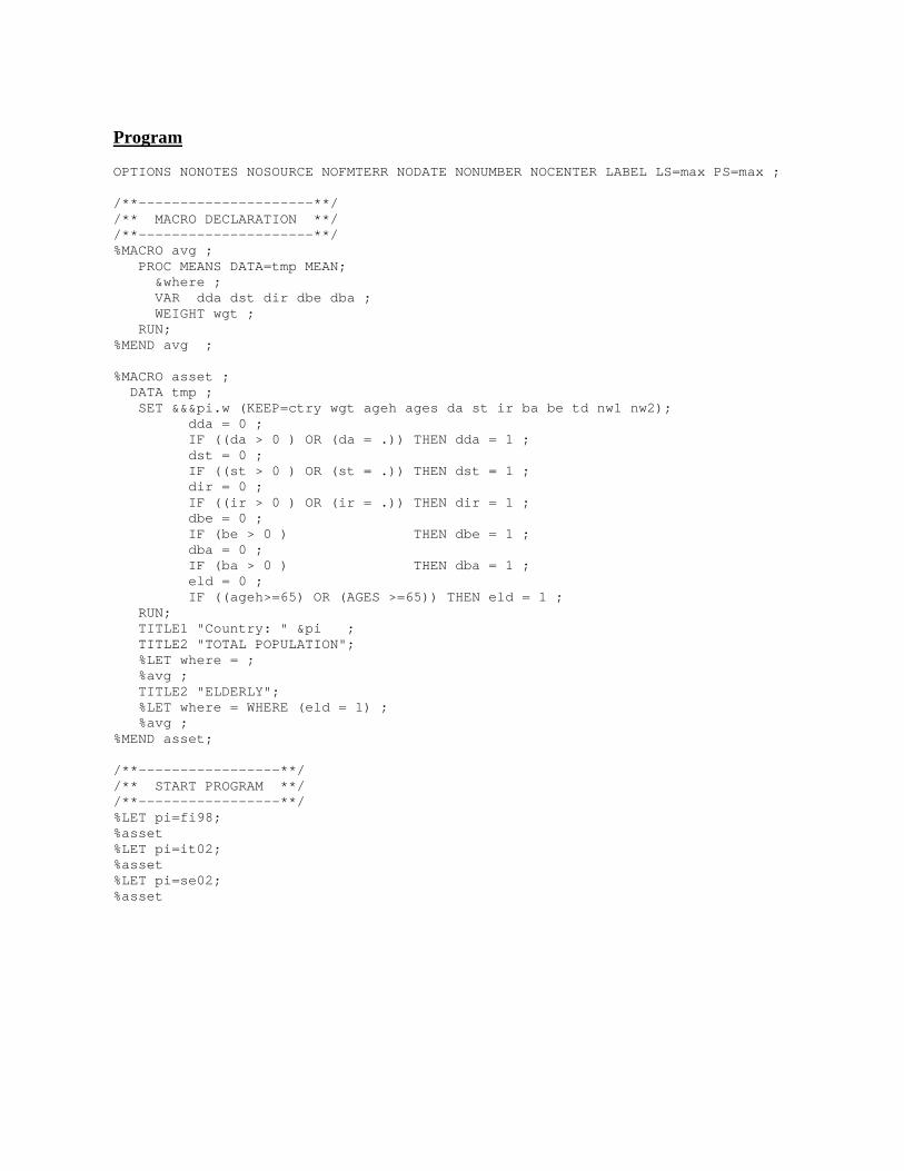
Program
OPTIONS NONOTES NOSOURCE NOFMTERR NODATE NONUMBER NOCENTER LABEL LS=max PS=max ; /**---------------------**/ /** MACRO DECLARATION **/ /**---------------------**/ %MACRO avg ; PROC MEANS DATA=tmp MEAN; &where ; VAR dda dst dir dbe dba ; WEIGHT wgt ; RUN; %MEND avg ; %MACRO asset ; DATA tmp ; SET &&&pi.w (KEEP=ctry wgt ageh ages da st ir ba be td nw1 nw2); dda = 0 ; IF ((da > 0 ) OR (da = .)) THEN dda = 1 ; dst = 0 ; IF ((st > 0 ) OR (st = .)) THEN dst = 1 ; dir = 0 ; IF ((ir > 0 ) OR (ir = .)) THEN dir = 1 ; dbe = 0 ; IF (be > 0 ) THEN dbe = 1 ; dba = 0 ; IF (ba > 0 ) THEN dba = 1 ; eld = 0 ; IF ((ageh>=65) OR (AGES >=65)) THEN eld = 1 ; RUN; TITLE1 "Country: " &pi ; TITLE2 "TOTAL POPULATION"; %LET where = ; %avg ; TITLE2 "ELDERLY"; %LET where = WHERE (eld = 1) ; %avg ; %MEND asset; /**-----------------**/ /** START PROGRAM **/ /**-----------------**/ %LET pi=fi98; %asset %LET pi=it02; %asset %LET pi=se02; %asset
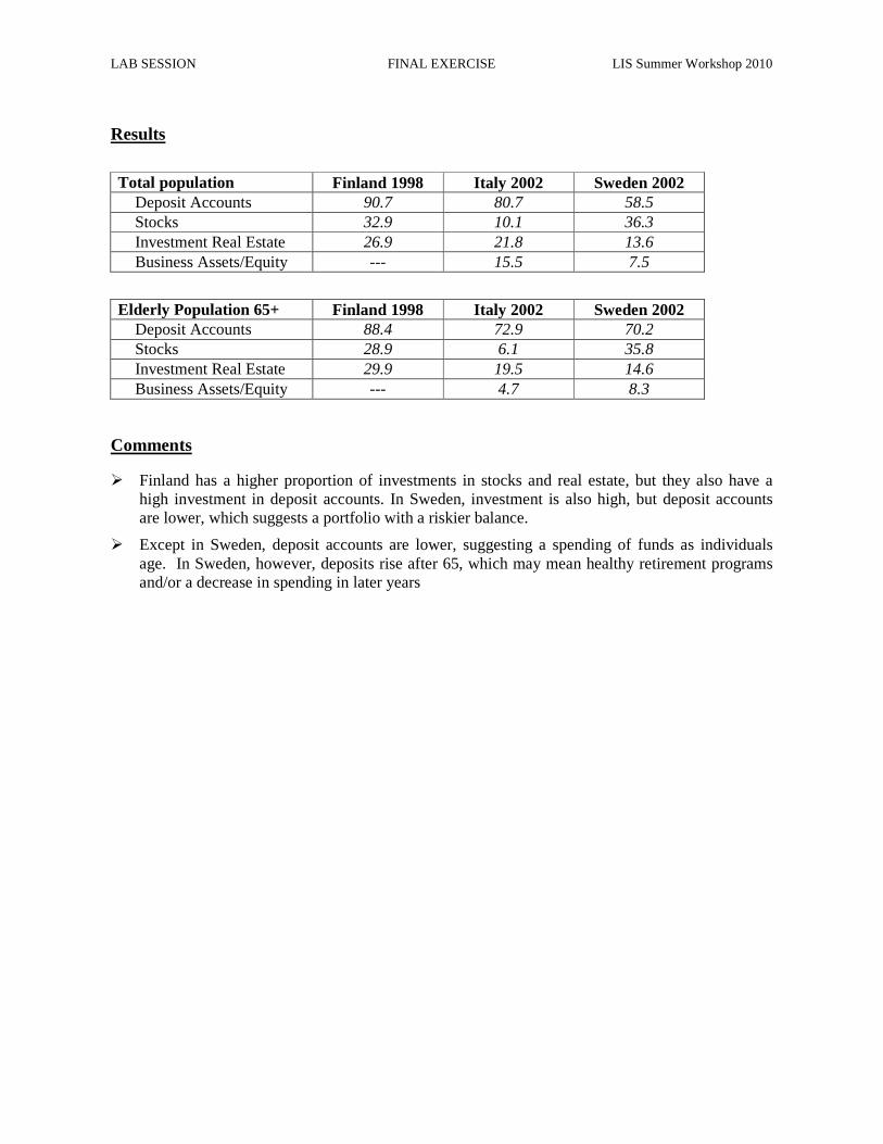
LAB SESSION FINAL EXERCISE LIS Summer Workshop 2010
Results
Total population Finland 1998 Italy 2002 Sweden 2002
Deposit Accounts 90.7 80.7 58.5 Stocks 32.9 10.1 36.3 Investment Real Estate 26.9 21.8 13.6 Business Assets/Equity --- 15.5 7.5
Elderly Population 65+ Finland 1998 Italy 2002 Sweden 2002
Deposit Accounts 88.4 72.9 70.2 Stocks 28.9 6.1 35.8 Investment Real Estate 29.9 19.5 14.6 Business Assets/Equity --- 4.7 8.3
Comments
� Finland has a higher proportion of investments in stocks and real estate, but they also have a high investment in deposit accounts. In Sweden, investment is also high, but deposit accounts are lower, which suggests a portfolio with a riskier balance.
� Except in Sweden, deposit accounts are lower, suggesting a spending of funds as individuals age. In Sweden, however, deposits rise after 65, which may mean healthy retirement programs and/or a decrease in spending in later years


![Introduction to SASmwatnik/sas_all2.pdf · Introduction to SAS The Statistical Analysis System [7], or SAS, is the package of record, as it is probably the most widely-used statistical](https://img.pdfslide.net/doc/110x75/5ec45c86e8f156666a719d1b/introduction-to-mwatniksasall2pdf-introduction-to-sas-the-statistical-analysis.jpg)