Embed Size (px)
DESCRIPTION
ymjlsdjfsdlifj jqwrhqureq3teyqwjrkle jweofjdslkjfjf dlfjsj wlej djf klsfjslfj s;dfn ejroe joejf e jfosejfoefjo gjdlgfgmkghj josejf sdlmfksdjfds fsdnkgj fjgojgodjgort7439uwoerg
Citation preview

------------------------------------------------------------------
Group members:
AINIL AFIQAH BT. MOHD HAMDANAUWATIF BT. U-UDEEB MAHFOUZ JAZOULY
NUR HAYATUL NISAB BT. MAT SARIP
Prepared for :
MR. MOHD NOOR AZAM B. NAFI
Group :
D2 CS221 5A

Introduction :
STA 610SAS Programming
• Source of Dataset : Journal of Statistics Education - Data Archive. (http://www.amstat.org/publications/jse/jse_data_archive.htm)
• This data set contains information for individual residential properties sold in Ames, Iowa from 2006 to 2010.
• Description of Dataset : See table
Introduction
Methodology
Result &
Analysis
Conclusion
Reference

Introduction :
STA 610SAS Programming
In order to conduct this project, we have set several
objectives:
a) To check model adequacy: normality, homogeneity
of variance and independency assumption.
b) To check the significance level of the model.
c) To identify if there is relationship between
dependent variable and independent variable.
Objectives :
Introduction
Methodology
Result &
Analysis
Conclusion
Reference
Introduction :
STA 610SAS Programming
In order to conduct this project, we have set several
objectives:
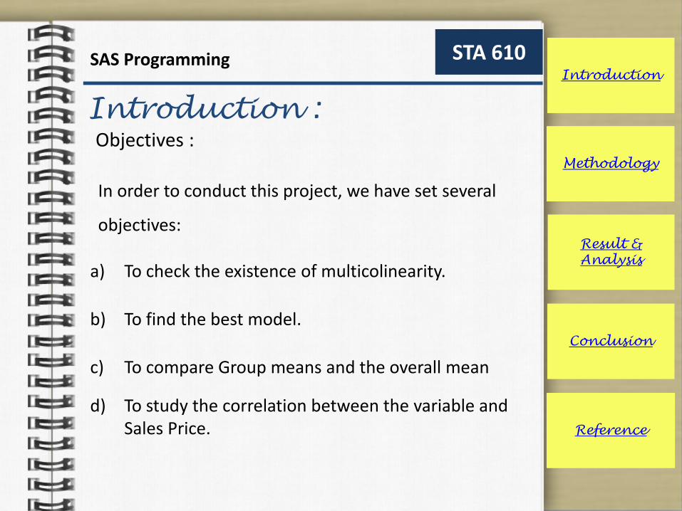
a) To check the existence of multicolinearity.
b) To find the best model.
c) To compare Group means and the overall mean
d) To study the correlation between the variable and Sales Price.
Objectives :
Introduction
Methodology
Result &
Analysis
Conclusion
Reference
Methodology :
Introduction
Methodology
STA 610SAS Programming
Result &
Analysis
Conclusion
Reference
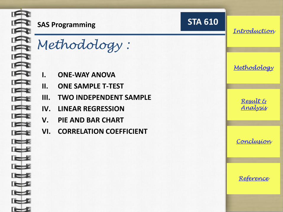
I. ONE-WAY ANOVA
II. ONE SAMPLE T-TEST
III. TWO INDEPENDENT SAMPLE
IV. LINEAR REGRESSION
V. PIE AND BAR CHART
VI. CORRELATION COEFFICIENT
Introduction
Methodology
Result &
Analysis
Conclusion
Reference
Result & Analysis :
Introduction
Methodology
STA 610SAS Programming
Result &
Analysis
Conclusion
Reference
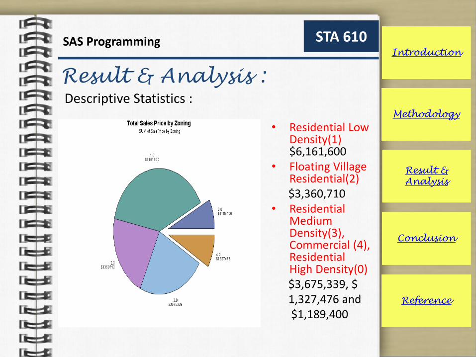
Descriptive Statistics :
• Residential Low Density(1) $6,161,600
• Floating Village Residential(2)$3,360,710
• Residential Medium Density(3), Commercial (4), Residential High Density(0)$3,675,339, $ 1,327,476 and $1,189,400
Introduction
Methodology
Result &
Analysis
Conclusion
Reference
Result & Analysis :
Introduction
Methodology
STA 610SAS Programming
Result &
Analysis
Conclusion
Reference
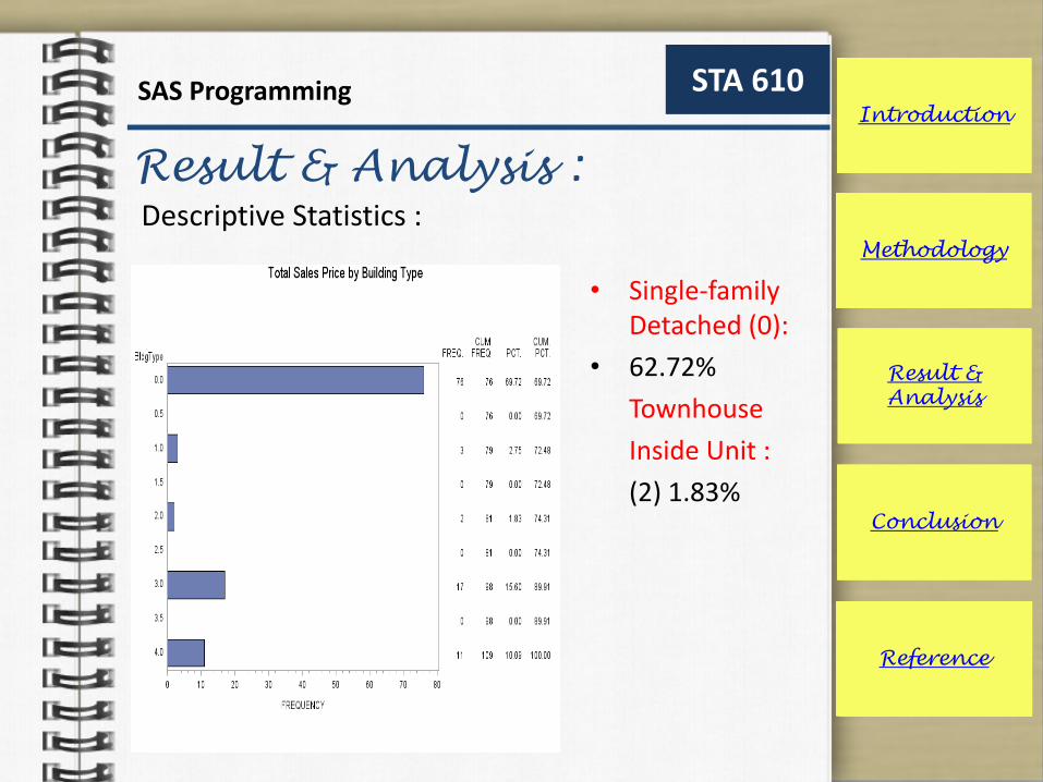
Descriptive Statistics :
• Single-family Detached (0):
• 62.72%
Townhouse
Inside Unit :
(2) 1.83%
Introduction
Methodology
Result &
Analysis
Conclusion
Reference

Result & Analysis :
Introduction
Methodology
STA 610SAS Programming
Result &
Analysis
Conclusion
Reference
Descriptive Statistics :
• Single-family Detached (0):
• 62.72%
Townhouse
Inside Unit :
(2) 1.83%
Introduction
Methodology
Result &
Analysis
Conclusion
Reference

Result & Analysis :
Introduction
Methodology
STA 610SAS Programming
Result &
Analysis
Conclusion
Reference
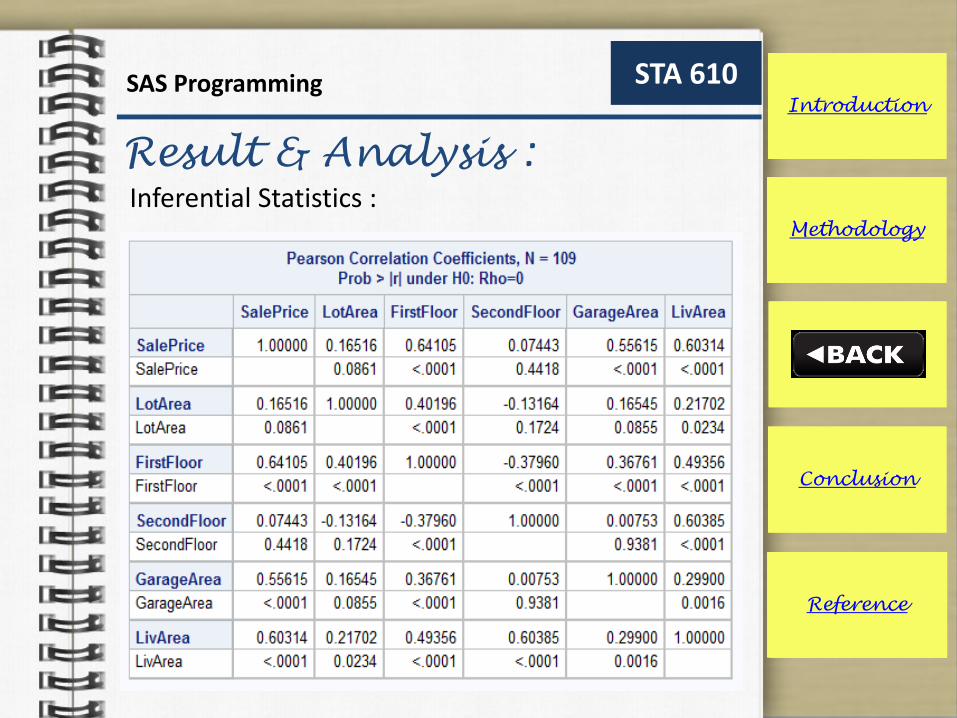
Inferential Statistics :
• to study the effect of Zoning, LotArea, FirstFloor, SecondFloor, GarageArea, LivArea, KitQual, BldgType variables on the SalesPrice.
• CORR procedure is required : computed Pearson correlation
• See output
Introduction
Methodology
Result &
Analysis
Conclusion
Reference
Result & Analysis :
Introduction
Methodology
STA 610SAS Programming
Result &
Analysis
Conclusion
Reference
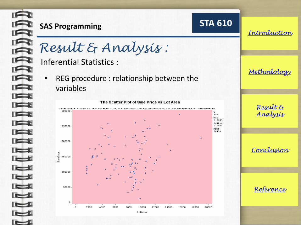
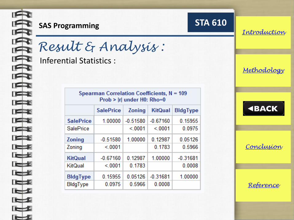
Inferential Statistics :
• REG procedure : relationship between the variables
Introduction
Methodology
Result &
Analysis
Conclusion
Reference

Result & Analysis :
Introduction
Methodology
STA 610SAS Programming
Result &
Analysis
Conclusion
Reference
Inferential Statistics :
• REG procedure : relationship between the variables
Introduction
Methodology
Result &
Analysis
Conclusion
Reference

Result & Analysis :
Introduction
Methodology
STA 610SAS Programming
Result &
Analysis
Conclusion
Reference
Inferential Statistics :
• REG procedure : relationship between the variables
Introduction
Methodology
Result &
Analysis
Conclusion
Reference

Result & Analysis :
Introduction
Methodology
STA 610SAS Programming
Result &
Analysis
Conclusion
Reference
Inferential Statistics :
• REG procedure : relationship between the variables
Introduction
Methodology
Result &
Analysis
Conclusion
Reference

Result & Analysis :
Introduction
Methodology
STA 610SAS Programming
Result &
Analysis
Conclusion
Reference
Inferential Statistics :
• REG procedure : relationship between the variables
Introduction
Methodology
Result &
Analysis
Conclusion
Reference

Result & Analysis :
Introduction
Methodology
STA 610SAS Programming
Result &
Analysis
Conclusion
Reference
Inferential Statistics :
• REG procedure : able to check the multicollinearity in the model .
• See ouput
Introduction
Methodology
Result &
Analysis
Conclusion
Reference

Result & Analysis :
Introduction
Methodology
STA 610SAS Programming
Result &
Analysis
Conclusion
Reference
Inferential Statistics :
• REG procedure : to check the model adequacy.
Normality Assumption :
Introduction
Methodology
Result &
Analysis
Conclusion
Reference
Result & Analysis :
Introduction
Methodology
STA 610SAS Programming
Result &
Analysis
Conclusion
Reference
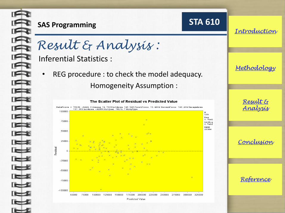
Inferential Statistics :
• REG procedure : to check the model adequacy.
Homogeneity Assumption :
Introduction
Methodology
Result &
Analysis
Conclusion
Reference

Result & Analysis :
Introduction
Methodology
STA 610SAS Programming
Result &
Analysis
Conclusion
Reference
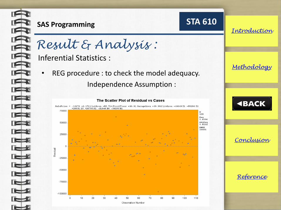
Inferential Statistics :
• REG procedure : to check the model adequacy.
Independence Assumption :
Introduction
Methodology
Result &
Analysis
Conclusion
Reference
Result & Analysis :
Introduction
Methodology
STA 610SAS Programming
Result &
Analysis
Conclusion
Reference
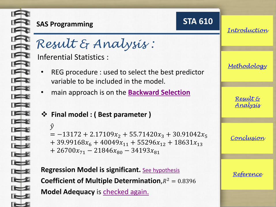
Inferential Statistics :
• REG procedure : used to select the best predictor variable to be included in the model.
• main approach is on the Backward Selection
Final model : ( Best parameter )
Regression Model is significant. See hypothesis
Coefficient of Multiple Determination,𝑅2 = 0.8396
Model Adequacy is checked again.
𝑦= −13172 + 2.17109𝑥2 + 55.71420𝑥3 + 30.91042𝑥5
+ 39.99168𝑥6 + 40049𝑥11 + 55296𝑥12 + 18631𝑥13
+ 26700𝑥71 − 21846𝑥80 − 34193𝑥81
Introduction
Methodology
Result &
Analysis
Conclusion
Reference
Result & Analysis :
Introduction
Methodology
STA 610SAS Programming
Result &
Analysis
Conclusion
Reference
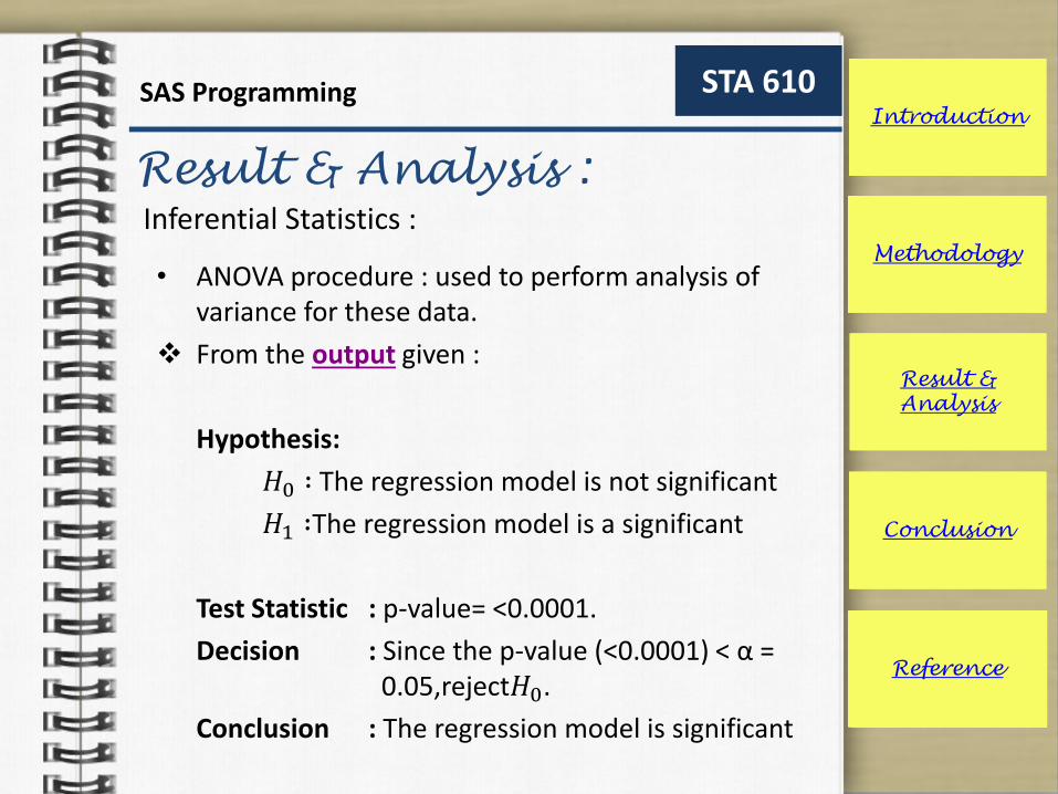
Inferential Statistics :
• ANOVA procedure : used to perform analysis of variance for these data.
From the output given :
Hypothesis:
𝐻0 ∶ The regression model is not significant
𝐻1 ∶The regression model is a significant
Test Statistic : p-value= <0.0001.
Decision : Since the p-value (<0.0001) < α = 0.05,reject𝐻0.
Conclusion : The regression model is significant
Introduction
Methodology
Result &
Analysis
Conclusion
Reference
Result & Analysis :
Introduction
Methodology
STA 610SAS Programming
Result &
Analysis
Conclusion
Reference
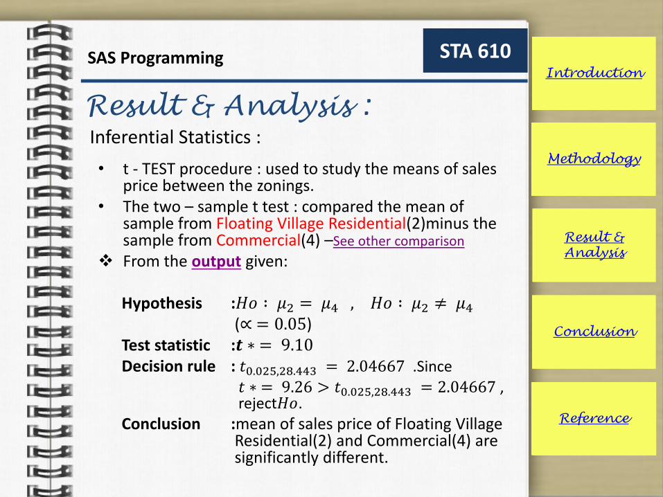
Inferential Statistics :
• t - TEST procedure : used to study the means of sales price between the zonings.
• The two – sample t test : compared the mean of sample from Floating Village Residential(2)minus the sample from Commercial(4) –See other comparison
From the output given:
Hypothesis :𝐻𝑜 ∶ 𝜇2 = 𝜇4 , 𝐻𝑜 ∶ 𝜇2 ≠ 𝜇4
(∝ = 0.05)Test statistic :𝒕 ∗ = 9.10Decision rule : 𝑡0.025,28.443 = 2.04667 .Since
𝑡 ∗ = 9.26 > 𝑡0.025,28.443 = 2.04667 , reject𝐻𝑜.
Conclusion :mean of sales price of Floating Village Residential(2) and Commercial(4) are significantly different.
Introduction
Methodology
Result &
Analysis
Conclusion
Reference

Result & Analysis :
Introduction
Methodology
STA 610SAS Programming
Result &
Analysis
Conclusion
Reference
Inferential Statistics :
• t - TEST procedure : used to study the overall mean given by the zonings – One Sampled t – Test
From the output given :
Hypothesis :𝐻𝑜: 𝜇 = $200,000 , 𝐻𝑜: 𝜇 ≠ $200,000(∝ = 0.05)
Test statistic :𝑝 − 𝑣𝑎𝑙𝑢𝑒 = < .0001
Decision rule : 𝑡0.025,228 = 2.05169 (Interpolation)
Since 𝑝 − 𝑣𝑎𝑙𝑢𝑒 = < .0001 < ∝ = 0.05, reject𝐻𝑜.
Conclusion : Mean of sales price is significantly different from $200,000.
Introduction
Methodology
Result &
Analysis
Conclusion
Reference
Conclusion :
Introduction
Methodology
STA 610SAS Programming
Result &
Analysis
Conclusion
Reference
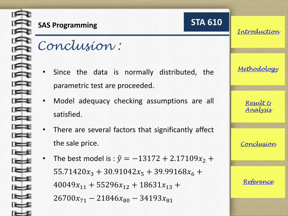
• Since the data is normally distributed, the
parametric test are proceeded.
• Model adequacy checking assumptions are all
satisfied.
• There are several factors that significantly affect
the sale price.
• The best model is : 𝑦 = −13172 + 2.17109𝑥2 +
55.71420𝑥3 + 30.91042𝑥5 + 39.99168𝑥6 +
40049𝑥11 + 55296𝑥12 + 18631𝑥13 +
26700𝑥71 − 21846𝑥80 − 34193𝑥81
Introduction
Methodology
Result &
Analysis
Conclusion
Reference

Reference :
Introduction
Methodology
STA 610SAS Programming
Result &
Analysis
Conclusion
Reference
• Buchecker, M., Calhoun, S. and Repole, W. (2004).
SAS Programming I: Essentials. USA: SAS Institute
Inc.
• Kutner, M. H.,Nachtsheim, C. J., Neter, J. and Li, W.
(2005). Applied Linear Statistical Models. New
York: McGraw Hill.
• Daniel W. W. (1990). Applied Nonparametric
Statistics. USA: Brooks/Cole Cengage Learning.

The End
Question & Answer

Output

Introduction :
Methodology
STA 610SAS Programming
Result &
Analysis
Conclusion
Reference
Variable Description Unit
X1=ZoningThe general zoning classification of the
sale.0 Residential High Density
1 Residential Low Density
2 Floating Village Residential
3 Residential Medium Density
4 Commercial
X2=LotArea Lot size Square feet (sqft)
X3=FirstFloor Area of First Floor Square feet (sqft)
X4=SecondFloor Area of Second Floor Square feet (sqft)
X5=GarageArea Area of garage Square feet (sqft)
X6=LivArea Size of living area Square feet (sqft)
X7=KitQual Kitchen quality 0 Excellent
1 Good
2 Typical/Average
X8=BldgType Type of building 0 Single-family Detached
1 Townhouse End Unit
2 Townhouse Inside Unit
3 Duplex
4 Two-family Conversion
Y=SalePrice Selling price Dollar ($)
Result & Analysis :
Introduction
Methodology
STA 610SAS Programming
Result &
Analysis
Conclusion
Reference
Inferential Statistics :
Introduction
Methodology
Conclusion
Reference
Result & Analysis :
Introduction
Methodology
STA 610SAS Programming
Result &
Analysis
Conclusion
Reference
Inferential Statistics :
Introduction
Methodology
Conclusion
Reference

Result & Analysis :
Introduction
Methodology
STA 610SAS Programming
Result &
Analysis
Conclusion
Reference
Inferential Statistics :
Introduction
Methodology
Conclusion
Reference
Result & Analysis :
Introduction
Methodology
STA 610SAS Programming
Result &
Analysis
Conclusion
Reference
Inferential Statistics :
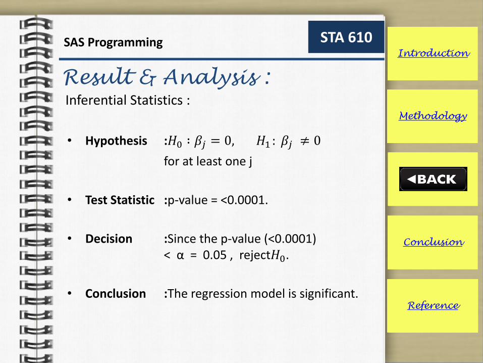
• Hypothesis :𝐻0 ∶ 𝛽𝑗 = 0, 𝐻1 : 𝛽𝑗 ≠ 0
for at least one j
• Test Statistic :p-value = <0.0001.
• Decision :Since the p-value (<0.0001) < α = 0.05 , reject𝐻0.
• Conclusion :The regression model is significant.
Introduction
Methodology
Result &
Analysis
Conclusion
Reference

Result & Analysis :
Introduction
Methodology
STA 610SAS Programming
Result &
Analysis
Conclusion
Reference
Inferential Statistics :
• REG procedure : to check the model adequacy.
Normality Assumption :
Introduction
Methodology
Conclusion
Reference

Result & Analysis :
Introduction
Methodology
STA 610SAS Programming
Result &
Analysis
Conclusion
Reference
Inferential Statistics :
• REG procedure : to check the model adequacy.
Homogeneity Assumption :
Introduction
Methodology
Conclusion
Reference
Result & Analysis :
Introduction
Methodology
STA 610SAS Programming
Result &
Analysis
Conclusion
Reference
Inferential Statistics :
• REG procedure : to check the model adequacy.
Independence Assumption :
Introduction
Methodology
Result &
Analysis
Conclusion
Reference

Result & Analysis :
Introduction
Methodology
STA 610SAS Programming
Result &
Analysis
Conclusion
Reference
Inferential Statistics :
Introduction
Methodology
Conclusion
Reference
The SAS System
The TTEST Procedure
Variable: SalePrice (SalePrice)
Zoning Method Mean 95% CL Mean Std Dev 95% CL StdDev
2 197689 174778 220600 44560.9 33187.6 67818.6
4 78086.8 62254.6 93919.0 30792.8 22933.5 46864.4
Diff (1-2) Pooled 119602 92842.8 146361 38300.6 30800.9 50659.9
Diff (1-2) Satterthwaite 119602 92711.0 146493
Method Variances DF t Value Pr > |t|
Pooled Equal 32 9.10 <.0001
Satterthwaite Unequal 28.443 9.10 <.0001
Cochran Unequal 16 9.10 <.0001

Result & Analysis :
Introduction
Methodology
STA 610SAS Programming
Result &
Analysis
Conclusion
Reference
Inferential Statistics :
Introduction
Methodology
Conclusion
Reference
Zoning t- value dft – tabulated
∝𝟐 = 𝟎. 𝟎𝟐𝟓
Decision Conclusion
0 and 1 -4.44 17.86 -2.10226Failed to
reject
𝐻𝑜
There are no
significant
differences
0 and 2 -4.95 21.99 -2.07406
0 and 3 0.03 15.642 2.12394
0 and 4 2.95 16.359 2.11641
Reject
𝐻𝑜
There are
significant
differences
1 and 2 -1.24 32.656 -2.03642
1 and 3 6.06 62.535 1.99916
1 and 4 9.56 44.307 2.01648
2 and 3 6.20 28.793 2.04562
2 and 4 9.10 28.443 2.04667
3 and 4 4.01 39.196 2.02269

Result & Analysis :
Introduction
Methodology
STA 610SAS Programming
Result &
Analysis
Conclusion
Reference
Inferential Statistics :
Introduction
Methodology
Conclusion
Reference
One - Mean Comparison of Sale Price Given BY Zoning
The TTEST Procedure
Variable: SalePrice (SalePrice)
Frequency: Zoning Zoning
N Mean Std Dev Std Err Minimum Maximum
229 127594 57758.0 3816.8 12789.0 289000
Mean 95% CL Mean Std Dev 95% CL StdDev
127594 120073 135114 57758.0 52908.2 63594.2
DF t Value Pr > |t|
228 -18.97 <.0001