Embed Size (px)
Citation preview
SATELLITE IMAGERY AND REMOTE SENSING METHODOLOGY:
APPLIED TO CHANGE DETECTION ALONG FOUNTAIN CREEK
by
Kristen Gilbert
;fefe.. '■^ZiSQ
Creative Investigation/Mini Thesis
April 17,1998
REPORT DOCUMENTATION PAGE Form Approved
OMB No. 0704-0188
Public reporting burden for this collection of information is estimated to average 1 hour per response, including the time for reviewing instructions, searching existing data sources, gathering and maintaining the data needed, and completing and reviewing the collection of information. Send comments regarding this burdBn estimate or any other aspect of this collection of information, including suggestions for reducing this burden, to Washington Headquarters Services, Directorate for Information Operations and Reports, 1215 JeffBrson Davis Highway, Suite 1204, Arlington, VA 222024302, and to the Office of Management and Budget, Paperwork Reduction Project (0704-0188), Washington, DC 20503.
1. AGENCY USE ONLY (Leaveblank) 2. REPORT DATE
26.Oct.98
3. REPORT TYPE AND DATES COVERED
MAJOR REPORT 4. TITLE AND SUBTITLE
SATELLITE IMAGERY AND REMOTE SENSING METHODOLOGY APPLIED TO CHANGE DETECTION ALONG FOUNTAIN CREEK
6. AUTHOR(S)
2D LT GILBERT KRISTEN L
5. FUNDING NUMBERS
7. PERFORMING ORGANIZATION NAME(S) AND ADDRESS(ES)
UNIVERSITY OF COLORADO AT COLORADO SPRINGS 8. PERFORMING ORGANIZATION
REPORT NUMBER
9. SPONSORING/MONITORING AGENCY NAME(S) AND ADDRESS(ES)
THE DEPARTMENT OF THE AIR FORCE AFIT/CIA, BLDG 125 2950 P STREET WPAFB OH 45433
10. SPONSORING/MONITORING AGENCY REPORT NUMBER
98-010
11. SUPPLEMENTARY NOTES
12a. DISTRIBUTION AVAILABILITY STATEMENT
Unlimited distribution In Accordance With AFI 35-205/AFIT Sup 1
12b. DISTRIBUTION CODE
13. ABSTRACT {Maximum 200 words!
14. SUBJECT TERMS 15. NUMBER OF PAGES
16. PRICE CODE
17. SECURITY CLASSIFICATION OF REPORT
18. SECURITY CLASSIFICATION OF THIS PAGE
19. SECURITY CLASSIFICATION OF ABSTRACT
20. LIMITATION OF ABSTRACT
Standard Form 298 (Rev. 2-89) (EG) Prescribed by ANSI Std. 239.18 Designed using Perform Pro, WHS/DIOR, Oct 94
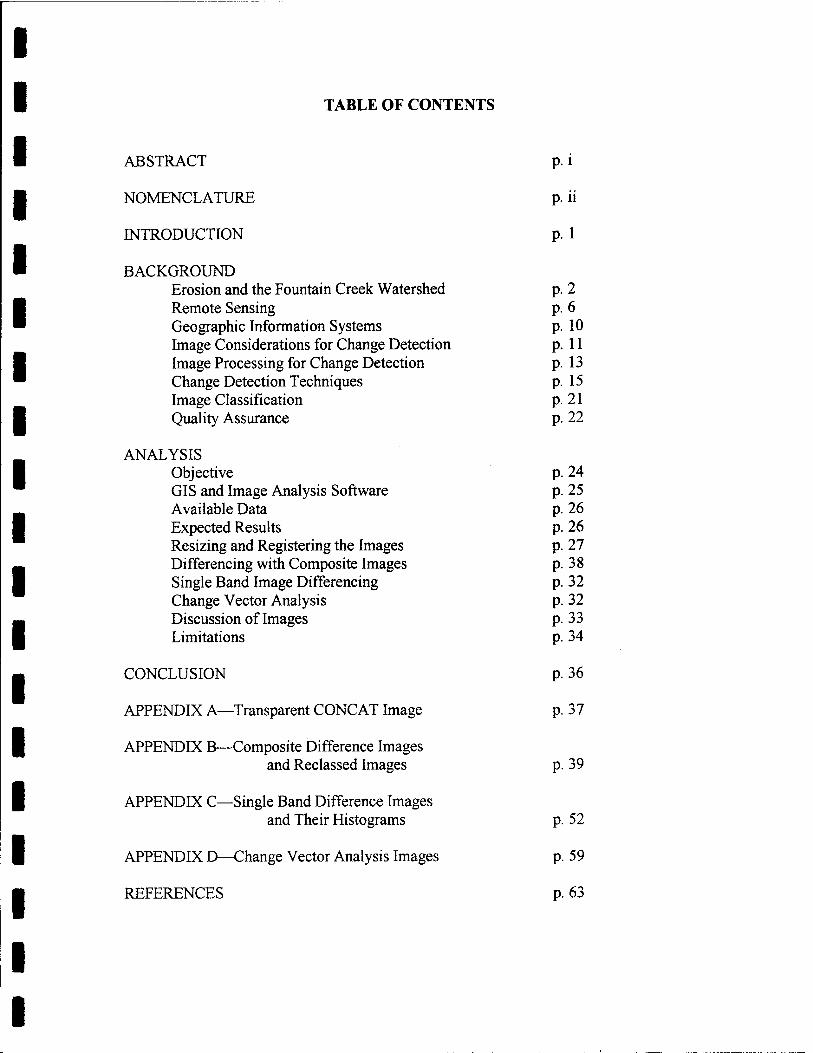
1 TABLE OF CONTENTS
1 ABSTRACT P-i
■ NOMENCLATURE p. ii
INTRODUCTION P-l
■ BACKGROUND Erosion and the Fountain Creek Watershed p. 2
I Remote Sensing p. 6 ■ Geographic Information Systems p. 10
Image Considerations for Change Detection p. 11 1 Image Processing for Change Detection p. 13 ™ Change Detection Techniques p. 15
Image Classification p. 21 ■ Quality Assurance p. 22
ANALYSIS I Objective p. 24
GIS and Image Analysis Software p. 25 _ Available Data p. 26 I Expected Results p. 26
Resizing and Registering the Images p. 27 — Differencing with Composite Images p. 38 ■ Single Band Image Differencing p. 32
Change Vector Analysis p. 32 B Discussion of Images p. 33 ■ Limitations p. 34
_ CONCLUSION p. 36
APPENDIX A—Transparent CONCAT Image p. 37
| APPENDIX B—Composite Difference Images and Reclassed Images p. 39
1 APPENDIX C—Single Band Difference Images and Their Histograms p. 52
| APPENDIX D—Change Vector Analysis Images p. 59
■ REFERENCES p. 63
ABSTRACT
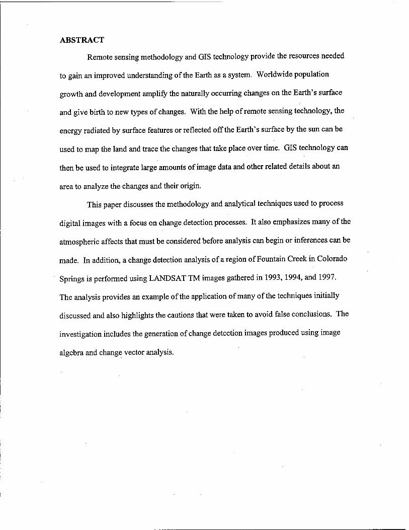
Remote sensing methodology and GIS technology provide the resources needed
to gain an improved understanding of the Earth as a system. Worldwide population
growth and development amplify the naturally occurring changes on the Earth's surface
and give birth to new types of changes. With the help of remote sensing technology, the
energy radiated by surface features or reflected off the Earth's surface by the sun can be
used to map the land and trace the changes that take place over time. GIS technology can
then be used to integrate large amounts of image data and other related details about an
area to analyze the changes and their origin.
This paper discusses the methodology and analytical techniques used to process
digital images with a focus on change detection processes. It also emphasizes many of the
atmospheric affects that must be considered before analysis can begin or inferences can be
made. In addition, a change detection analysis of a region of Fountain Creek in Colorado
Springs is performed using LANDSAT TM images gathered in 1993, 1994, and 1997.
The analysis provides an example of the application of many of the techniques initially
discussed and also highlights the cautions that were taken to avoid false conclusions. The
investigation includes the generation of change detection images produced using image
algebra and change vector analysis.
NOMENCLATURE
C-CAP Coastal Change Analysis Program
DEM Digital Elevation Model
DN Digital Number
FCWP Fountain Creek Watershed Project
GCP Ground Control Point
GIS Geographic Information System
IFOV Instantaneous Field of View
MSS Multispectral Scanner
NASA National Aeronautics and Space Administration
TM Thematic Mapper
USGS United States Geological Survey
INTRODUCTION
Humans have roamed the Earth for many years, forming habitats and
experiencing, if not causing, an innumerable amount of changes in the Earth's surface
features. Thus, it is only natural to wonder how the surface changes and to analyze the
occurrences and causes of that change.
The integration of remote sensing and GIS technology provides a unique and
effective method of monitoring and analyzing the changes that occur on the Earth's
surface. While some features remain relatively stable over time, much of the Earth's
surface constantly changes due to natural processes or man-made disturbances.
Therefore, an accurate and consistent inventory of the changes, in the form of images,
helps illustrate the dynamics of the change and clarifies its source. A multitude of
information gathering tools and analysis techniques exist to perform investigations of the
physical processes at work. Images can be created to facilitate the evaluation of
deforestation, desertification, contamination, and erosion and help clarify the possible
causes of such change. Furthermore, the information gathered from remotely sensed
images aids the decision-making processes related to crop yields and health, land use,
project site evaluation, forest management, and hydrology. These research techniques
provide one focus of this investigative report. This paper also demonstrates the use of
several of these techniques as they apply to the analysis of the erosion along Fountain
Creek.
BACKGROUND
Erosion and the Fountain Creek Watershed
The Fountain Creek region of Colorado is one of many areas in the United States
and foreign nations that faces challenges due to flooding and erosion. As a result of the
concerns, several government and private organizations have been developed to improve
the management of streams, rivers, and floodplains, and to pursue the restoration of such
areas when and if possible. The Interagency Floodplain Management Committee and the
Coalition to Restore Aquatic Ecosystems are examples of such organizations. In
addition, local advocacy groups for rivers and streams have surfaced, such as River
Watch in Illinois and the Stream Teams in Missouri, and now receive funding and
technical assistance from regional or state programs. Likewise, the Fountain Creek
Watershed Project, made up of concerned residents, professionals, and government
officials, currently works to resolve the issues created by the Fountain Creek
transformation.
Like the Fountain Creek area, numerous countries worldwide suffer from the
challenges related to watersheds. The following two examples demonstrate the
prevalence of the problem worldwide and the similarity of the underlying causes as
compared to Fountain Creek. The first case occurs in the Jhiku Khola watershed in
Nepal. The problems of the Jhiku Khola watershed originate with its erosion prone red
soil, typical of the Middle Mountains. On top ofthat, increased farming and grazing, and
influx of migrants during the monsoon season augment the dilemma. The presence of
human activities in the area causes soil erosion, sedimentation, deforestation, and a
reduction in the fertility of the soil. [1]
Similarly, a study of the Missouri River Floodplain, conducted in 1983, concluded
that the many human activities in the floodplain contribute to the damage that the area
encounters. Bank stabilization and navigation structures along the river constrict the
floodplain and lead to the accretion of land along the channel. Furthermore, development
projects and highway and railway embankments in the floodplain introduce unnatural
environmental conditions that magnify the flooding and erosion problems. [2]
The cases above introduce three of the major factors contributing to the watershed
dilemma—growing populations, forest clearing, and land development. These
interrelated circumstances send large amounts of sediment and other pollutants into the
waterway and facilitate the process of erosion. A quantitative analysis of this relationship
shows that once ten percent of a watershed (particularly the upper region) is paved over
or compacted, the waterway progressively degrades. The river channels are cut deeper
and deeper by increased water loads and flooding becomes more frequent [3]. These
same factors are exactly what make Fountain Creek "one of the worst creeks in the state
[of Colorado] for bank erosion [4]."
The city of Colorado Springs and the surrounding area, including the Pikes Peak
region and extending south towards Pueblo, has undergone a transformation in recent
years leading to a magnification of the erosive processes along Fountain Creek. Before
the 1950's, when there were fewer people and fewer developed areas, Fountain Creek
flowed for part of the year, drying up late in the summer and staying dry during the
winter. Now, the creek flows nonstop. It started rising as a result of more water flowing
into the creek from booming development, more paved streets and accompanying
drainage systems, and increasing amounts of household water pumped into the area [4].
Increased rainwater and the region's fragile sandy soils add to the dilemma. Currently,
the water flowing through Fountain Creek carries approximately 70 truckloads of
sediment into the Arkansas River daily. The creek's water flow has the power to rip soils
from its banks and its bottom, as well as destroy pipelines, trails, homes, bridges, roads,
and railroad tracks. In fact, the creek's path can move up to 100 feet per year in some
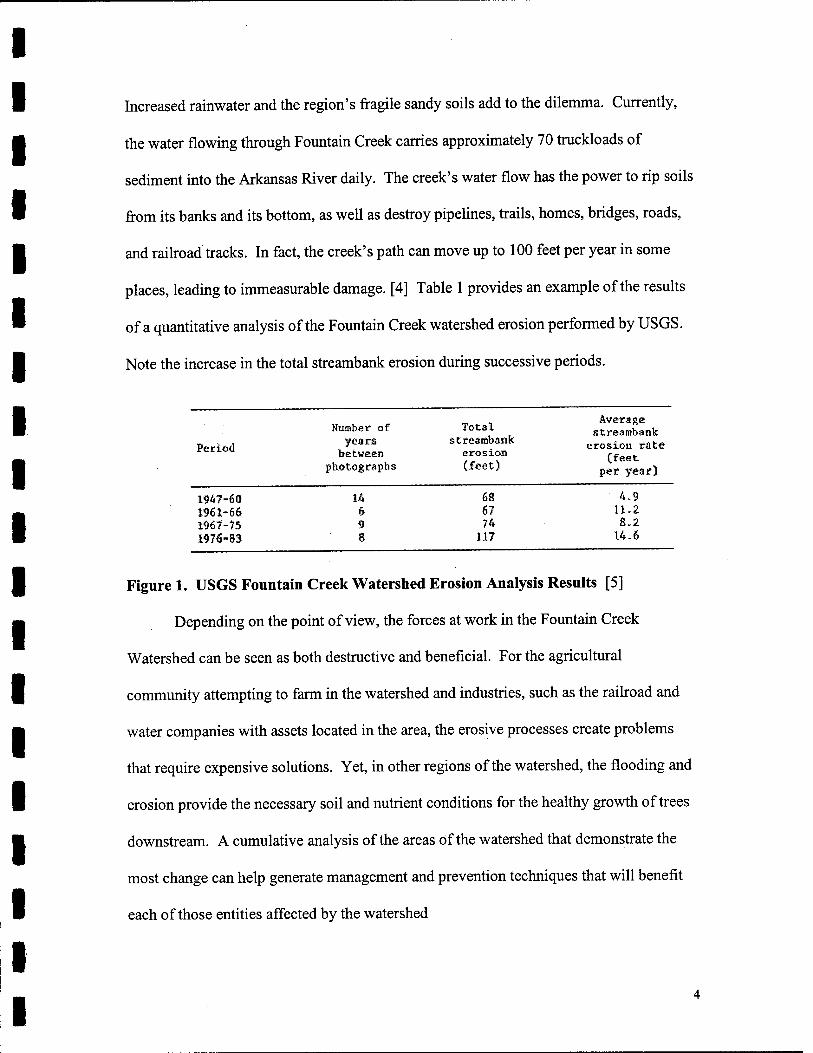
places, leading to immeasurable damage. [4] Table 1 provides an example of the results
of a quantitative analysis of the Fountain Creek watershed erosion performed by USGS.
Note the increase in the total streambank erosion during successive periods.
Average streambank
peri0(i , J™1" """'T* erosion rate
Number of Total years streambank
between erosion photographs (feet)
(feet per year)
1947-60 1961-66 1967-75 I976-S3
14 68 4,9 6 67 11.2 9 74 8.2 8 117 14.6
Figure 1. USGS Fountain Creek Watershed Erosion Analysis Results [5]
Depending on the point of view, the forces at work in the Fountain Creek
Watershed can be seen as both destructive and beneficial. For the agricultural
community attempting to farm in the watershed and industries, such as the railroad and
water companies with assets located in the area, the erosive processes create problems
that require expensive solutions. Yet, in other regions of the watershed, the flooding and
erosion provide the necessary soil and nutrient conditions for the healthy growth of trees
downstream. A cumulative analysis of the areas of the watershed that demonstrate the
most change can help generate management and prevention techniques that will benefit
each of those entities affected by the watershed
Controversy over how to deal with watershed issues arises from the numerous
individuals affected by the disastrous flooding and erosion and the economic predicament
that ensues. In one case, 201 farmers in the Minnesota River watershed were paid a total
of $7.6 million after the floods in 1993 to convert 9200 acres of their low lying farmland
into permanent conservation easements. Now the land that was once planted in crops is
covered with grasses and trees that are less vulnerable to erosion and, hence, the risk of
expensive losses has been greatly reduced [6]. Regardless, the government had to dish
out a large sum of money to correct the problem. In the case of Fountain Creek, a gas
company spent $500,000 trying to protect a pipeline from bank erosion, but eventually
had to remove it. Likewise, a railroad company spent $500,000 to rebuild a creek bank
after water eroded the track's supporting soil. These examples clearly illustrate the
economic burden and hardship that some industries face in regions like the Fountain
Creek Watershed, but how to resolve the problems remains a mystery.
Many proposals have been made to suggest methods for curbing the erosion along
rivers and creeks. Two of these include lining the creek with boulders and trees, and
building expensive reservoir systems to help reduce the abrupt flow of stormwater into
the creek. The planting of trees along riverbeds has been tried and proven worldwide.
The network of roots that trees provide helps control erosion and removes excess
nutrients and sediments from incoming groundwater [7]. Unfortunately, in the case of
Fountain Creek, the results were not so impressive. Tom Johnson, director of FCWP,
planted trees along a portion of the creek to test the feasibility of the option. He chose a
type of tree that develops extensive root systems and grows unusually quickly, hoping
that the trees would withstand the creek's power and stabilize the fragile soils. However,
the trees could not combat the compound forces present along Fountain Creek. Likewise,
while placing boulders along the creek's edge protects the immediate stream bank from
strong currents, future problems arise when the water inevitably displaces the boulders.
Flowing water then bounces off the large objects in its path, giving it more energy and
causing more intense erosion downstream [4]. Other preventative techniques that have
been suggested, such as lining the creek with concrete, also prove to be either more
destructive or impractical. Hence, the search for a steadfast solution continues.
Investigations such as this one may set a foundation to help prevent any further
wastes of money and resources due to the erosive processes in watershed regions.
Consequently, the FCWP hopes to benefit from the results of this study by gaining more
insight into their problem and bringing them one step closer to a possible solution. In
addition, the scientific community may be interested in the results of this investigation as
it provides another example of the information that can be derived by integrating
remotely sensed images with GIS technology.
Remote Sensing
Remote sensing is defined as the process of obtaining information about an object
by acquiring data with a device that is not in contact with that object [8], e.g. satellites,
cameras, the human eye. Before the advent of remote sensing, there was no efficient
method of gathering a clear, consistent record of ground features and observable surface
changes. Yet, satellite imagery and aerial photography now provide the means to make
comparisons of images over time.
Both the remote sensing methodology and the imagery data offer several benefits
when used as analytical tools for the study of the Earth's changing surface features. First,
satellites provide the vehicle necessary to carry large sensors over large coverage areas
on a repetitive basis. This means that satellite imagery is internally consistent through
time-the same location can be re-examined by a sensor at different known intervals [9],
depending on the satellite's orbit. This repetitive coverage permits the tracking of
changes over a desired region or time frame. Furthermore, simulation models such as
ADAPT and WEPP, which were often used in the past, get the job done, but are time
consuming, labor intensive, and costly [10]. The simulation models also require
destructive sampling to acquire ground truth data. Remote sensing techniques, on the
other hand, provide fast, low cost information and are non-destructive; although ground
sampling may improve analysis, it is not required. Furthermore, the wide-area coverage
of satellites is a particularly important advantage when studying large areas, such as
lengthy waterways. All in all, remote sensing technology cuts data-gathering costs and
improves forecasting of long-term consequences of urban development [11]. As a result,
many county and state governments currently use LANDSAT and SPOT satellite data for
change analyses.
There are two types of remote sensing data that can be gathered: active and
passive. Active remote sensing involves the use of radar satellites. A radar satellite
sends a known signal to Earth and then another sensor on board the satellite measures the
return signal, which it uses to create a map of ground features. On the other hand,
passive remote sensing equipment measures incoming energy reflected from the sun off
an object or the energy emitted by the object itself to create an image. Since all objects
emit electromagnetic energy, passive remote sensing provides an efficient means of
gathering spectral data and will be the type of data used in the investigation of Fountain
Creek.
Besides the type of data, three attributes of remote sensing systems must be
considered to determine the most advantageous system for a given analysis. (1) Spatial
resolution is the level of detail or the size of the smallest identifiable object. Present
sensors for use by the public generally provide between 30-meter and 4-kilometer
resolution. Most of the imagery used in this study has 30-meter resolution. (2) The
number of different colors or parts of the spectrum that a system measures defines its
spectral coverage. Today's systems are capable of supplying one to seven
measurements. Since electromagnetic energy measured at different wavelengths reveals
more details than only visible light, multispectral satellite images are often preferred over
aerial photographs. As such, this study will use LANDSAT multispectral images. (3)
Temporal frequency describes how often a sensor collects data over the desired region.
Current systems' cycles range from one image per month to two images per day. [8] The
imagery from the LANDSAT TM sensor will be the primary sensor of concern for the
remainder of the report since the Fountain Creek analysis employs such data.
The LANDSAT TM sensor was designed to improve upon the shortcomings of
the LANDSAT MSS equipment. The TM sensor images a 185 kilometer swath and
returns to a given area every 16 days. Furthermore, LANDSAT TM images provide 30-
meter ground resolution, except for the thermal band which has a resolution of 120-
meters. More importantly, TM sensors provide information from seven different spectral
bands. The wavelength range and location of the bands were chosen to improve the
capability to discriminate between major Earth surface features. Table 2 shows the
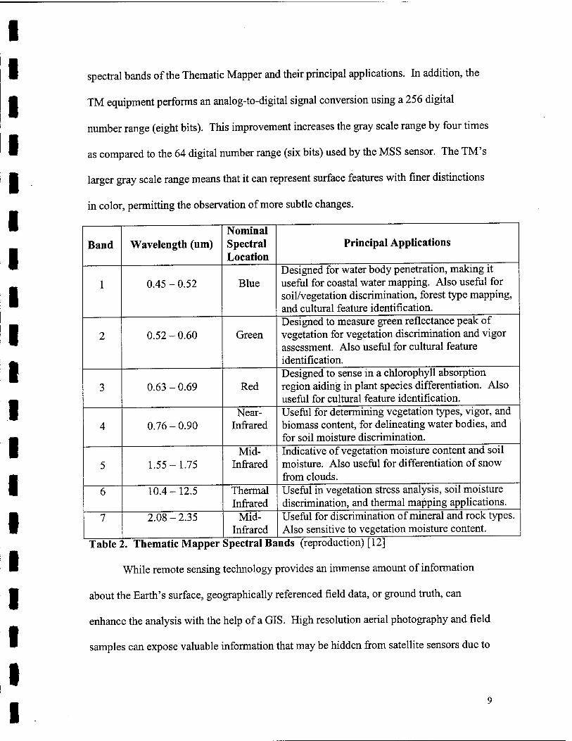
spectral bands of the Thematic Mapper and their principal applications. In addition, the
TM equipment performs an analog-to-digital signal conversion using a 256 digital
number range (eight bits). This improvement increases the gray scale range by four times
as compared to the 64 digital number range (six bits) used by the MSS sensor. The TM's
larger gray scale range means that it can represent surface features with finer distinctions
in color, permitting the observation of more subtle changes.
Band Wavelength (um) Nominal Spectral Location
Principal Applications
1 0.45 - 0.52 Blue Designed for water body penetration, making it useful for coastal water mapping. Also useful for soil/vegetation discrimination, forest type mapping, and cultural feature identification.
2 0.52 - 0.60 Green Designed to measure green reflectance peak of vegetation for vegetation discrimination and vigor assessment. Also useful for cultural feature identification.
3 0.63-0.69 Red Designed to sense in a chlorophyll absorption region aiding in plant species differentiation. Also useful for cultural feature identification.
4 0.76 - 0.90 Near-
Infrared Useful for determining vegetation types, vigor, and biomass content, for delineating water bodies, and for soil moisture discrimination.
5 1.55-1.75 Mid-
Infrared Indicative of vegetation moisture content and soil moisture. Also useful for differentiation of snow from clouds.
6 10.4-12.5 Thermal Infrared
Useful in vegetation stress analysis, soil moisture discrimination, and thermal mapping applications.
7 2.08-2.35 Mid- Infrared
Useful for discrimination of mineral and rock types. Also sensitive to vegetation moisture content.
Table 2. Thematic Mapper Spectral Bands (reproduction) [12]
While remote sensing technology provides an immense amount of information
about the Earth's surface, geographically referenced field data, or ground truth, can
enhance the analysis with the help of a GIS. High resolution aerial photography and field
samples can expose valuable information that may be hidden from satellite sensors due to
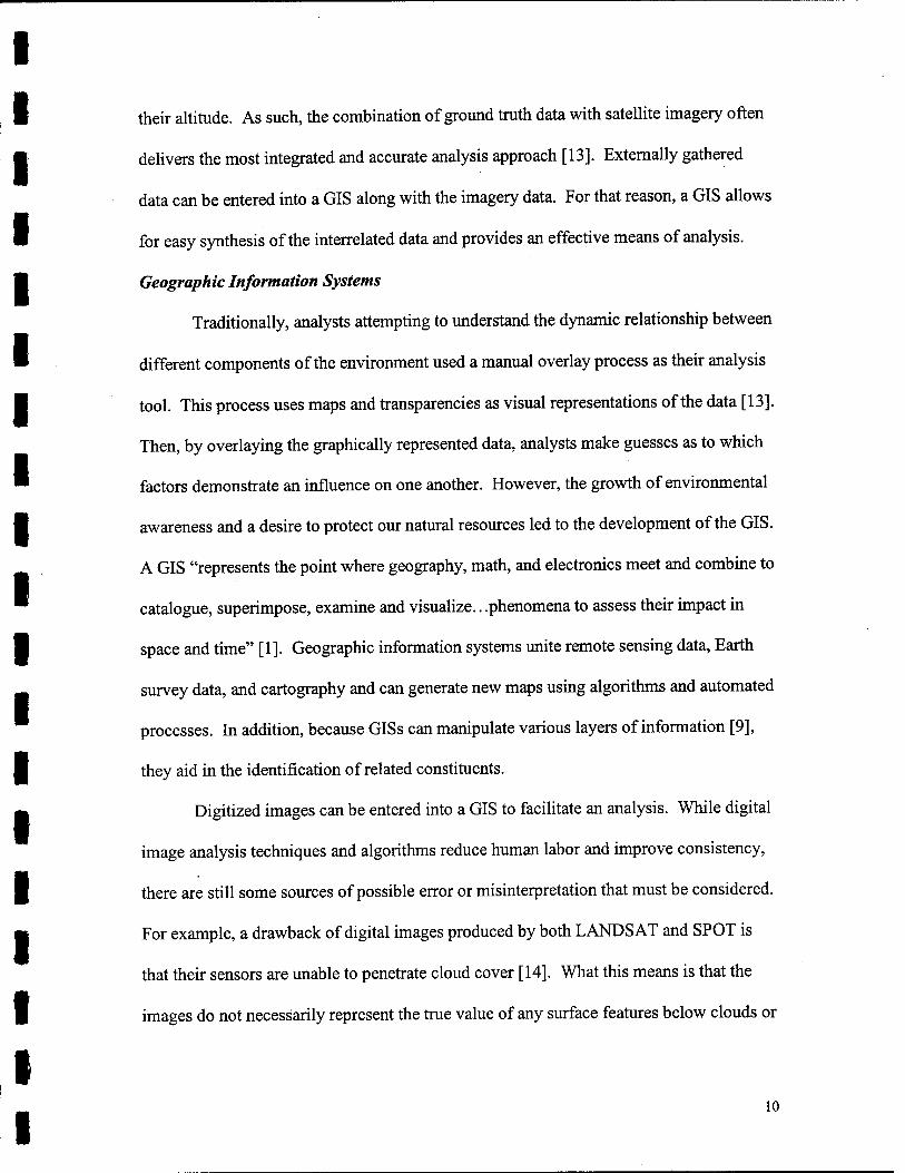
their altitude. As such, the combination of ground truth data with satellite imagery often
delivers the most integrated and accurate analysis approach [13]. Externally gathered
data can be entered into a GIS along with the imagery data. For that reason, a GIS allows
for easy synthesis of the interrelated data and provides an effective means of analysis.
Geographic Information Systems
Traditionally, analysts attempting to understand the dynamic relationship between
different components of the environment used a manual overlay process as their analysis
tool. This process uses maps and transparencies as visual representations of the data [13].
Then, by overlaying the graphically represented data, analysts make guesses as to which
factors demonstrate an influence on one another. However, the growth of environmental
awareness and a desire to protect our natural resources led to the development of the GIS.
A GIS "represents the point where geography, math, and electronics meet and combine to
catalogue, superimpose, examine and visualize.. .phenomena to assess their impact in
space and time" [1]. Geographic information systems unite remote sensing data, Earth
survey data, and cartography and can generate new maps using algorithms and automated
processes. In addition, because GISs can manipulate various layers of information [9],
they aid in the identification of related constituents.
Digitized images can be entered into a GIS to facilitate an analysis. While digital
image analysis techniques and algorithms reduce human labor and improve consistency,
there are still some sources of possible error or misinterpretation that must be considered.
For example, a drawback of digital images produced by both LANDS AT and SPOT is
that their sensors are unable to penetrate cloud cover [14]. What this means is that the
images do not necessarily represent the true value of any surface features below clouds or
10
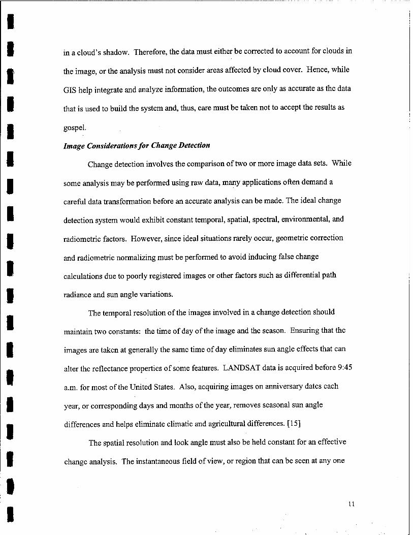
in a cloud's shadow. Therefore, the data must either be corrected to account for clouds in
the image, or the analysis must not consider areas affected by cloud cover. Hence, while
GIS help integrate and analyze information, the outcomes are only as accurate as the data
that is used to build the system and, thus, care must be taken not to accept the results as
gospel.
Image Considerations for Change Detection
Change detection involves the comparison of two or more image data sets. While
some analysis may be performed using raw data, many applications often demand a
careful data transformation before an accurate analysis can be made. The ideal change
detection system would exhibit constant temporal, spatial, spectral, environmental, and
radiometric factors. However, since ideal situations rarely occur, geometric correction
and radiometric normalizing must be performed to avoid inducing false change
calculations due to poorly registered images or other factors such as differential path
radiance and sun angle variations.
The temporal resolution of the images involved in a change detection should
maintain two constants: the time of day of the image and the season. Ensuring that the
images are taken at generally the same time of day eliminates sun angle effects that can
alter the reflectance properties of some features. LANDSAT data is acquired before 9:45
a.m. for most of the United States. Also, acquiring images on anniversary dates each
year, or corresponding days and months of the year, removes seasonal sun angle
differences and helps eliminate climatic and agricultural differences. [15]
The spatial resolution and look angle must also be held constant for an effective
change analysis. The instantaneous field of view, or region that can be seen at any one
11
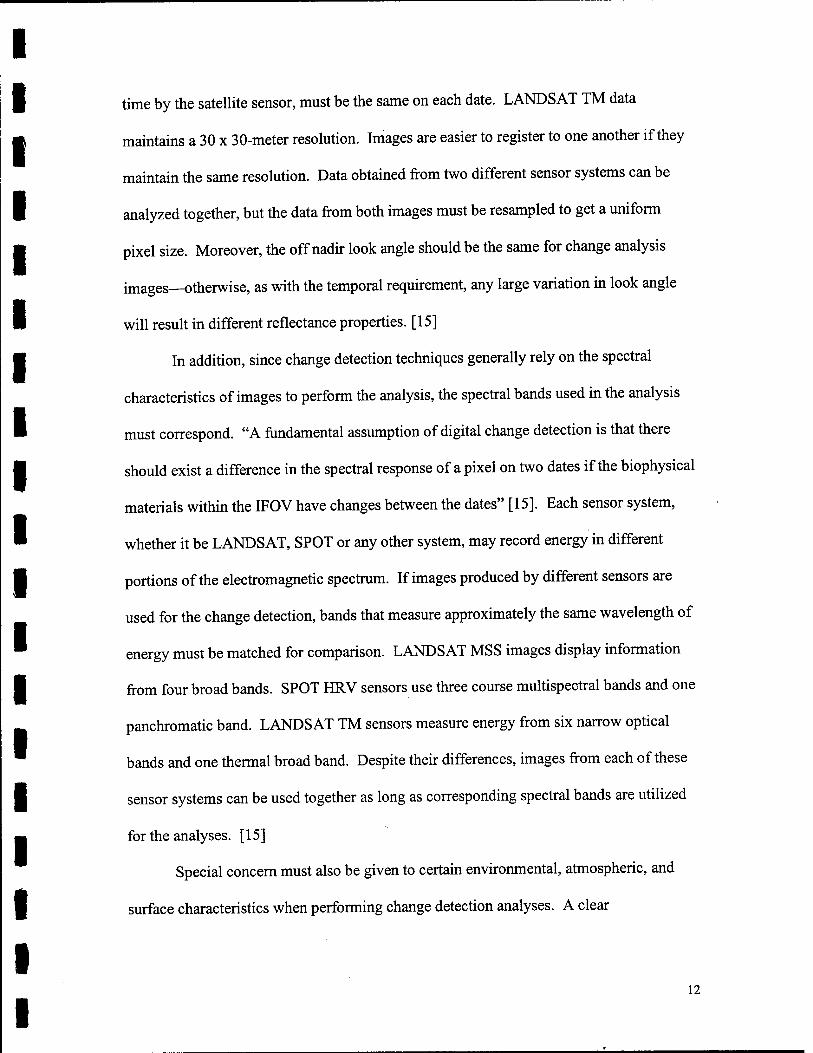
time by the satellite sensor, must be the same on each date. LANDSAT TM data
maintains a 30 x 30-meter resolution. Images are easier to register to one another if they
maintain the same resolution. Data obtained from two different sensor systems can be
analyzed together, but the data from both images must be resampled to get a uniform
pixel size. Moreover, the off nadir look angle should be the same for change analysis
images—otherwise, as with the temporal requirement, any large variation in look angle
will result in different reflectance properties. [15]
In addition, since change detection techniques generally rely on the spectral
characteristics of images to perform the analysis, the spectral bands used in the analysis
must correspond. "A fundamental assumption of digital change detection is that there
should exist a difference in the spectral response of a pixel on two dates if the biophysical
materials within the IFOV have changes between the dates" [15]. Each sensor system,
whether it be LANDSAT, SPOT or any other system, may record energy in different
portions of the electromagnetic spectrum. If images produced by different sensors are
used for the change detection, bands that measure approximately the same wavelength of
energy must be matched for comparison. LANDSAT MSS images display information
from four broad bands. SPOT HRV sensors use three course multispectral bands and one
panchromatic band. LANDSAT TM sensors measure energy from six narrow optical
bands and one thermal broad band. Despite their differences, images from each of these
sensor systems can be used together as long as corresponding spectral bands are utilized
for the analyses. [15]
Special concern must also be given to certain environmental, atmospheric, and
surface characteristics when performing change detection analyses. A clear
12
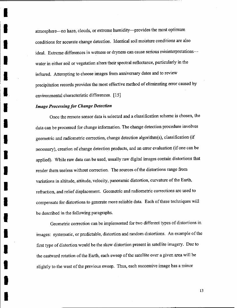
atmosphere—no haze, clouds, or extreme humidity—provides the most optimum
conditions for accurate change detection. Identical soil moisture conditions are also
ideal. Extreme differences in wetness or dryness can cause serious misinterpretations—
water in either soil or vegetation alters their spectral reflectance, particularly in the
infrared. Attempting to choose images from anniversary dates and to review
precipitation records provides the most effective method of eliminating error caused by
environmental characteristic differences. [15]
Image Processing for Change Detection
Once the remote sensor data is selected and a classification scheme is chosen, the
data can be processed for change information. The change detection procedure involves
geometric and radiometric correction, change detection algorithm(s), classification (if
necessary), creation of change detection products, and an error evaluation (if one can be
applied). While raw data can be used, usually raw digital images contain distortions that
render them useless without correction. The sources of the distortions range from
variations in altitude, attitude, velocity, panoramic distortion, curvature of the Earth,
refraction, and relief displacement. Geometric and radiometric corrections are used to
compensate for distortions to generate more reliable data. Each of these techniques will
be described in the following paragraphs.
Geometric correction can be implemented for two different types of distortions in
images: systematic, or predictable, distortion and random distortions. An example of the
first type of distortion would be the skew distortion present in satellite imagery. Due to
the eastward rotation of the Earth, each sweep of the satellite over a given area will be
slightly to the west of the previous sweep. Thus, each successive image has a minor
13
offset that must be corrected before an accurate analysis can be made. This type of
systematic offset is easily correctable using mathematical relationships.
Ground control points provide a basis for correcting random distortions. Ground
control points are "features of known ground location that can be accurately located on
the digital imagery" [12], such as buildings, highway intersections, and distinct
shorelines. A least squares regression analysis is accomplished using the GCPs digital
coordinates and their known geographic coordinates. The result of the least squares
yields the coefficients of the coordinate transformation equations necessary for realigning
the distorted image [12]. The Fountain Creek analysis will also demonstrate how GCPs
can be used for registering or aligning different images to one another.
Depending on the application at hand, radiometric correction may be necessary if
the radiance measured by the sensor varies due to scene illumination, atmospheric
conditions, viewing geometry, or inaccurate instrumentation. The radiometric correction
technique presented here provides an example of how to correct for the change in
reflectance of ground features at different times or locations [12]. First, the brightness of
each pixel is calculated based on a zenith sun angle for each image. Then, each pixel is
divided by the sine of the solar elevation angle for the appropriate time and location of a
given image to provide a better representation of the true radiance. Again, this simple
technique specifically accounts for seasonal variations in the sun angle.
Several resampling algorithms can also be used to correct multi-date data:
bilinear interpolation, nearest neighbor, and cubic convolution. Each of these methods
provides a means for registering imagery data in a GIS and can be used to prepare multi-
14
date images for overlay analysis. The algorithms are described in the following
paragraphs.
The popularity of the nearest neighbor technique emanates from the simplicity of
its calculations. This algorithm assigns any unknown pixel the value of the closest pixel
in the sampling grid. This method of reassignment retains the original pixel brightness
values throughout the transformation of the image. However, the algorithm can produce
images with less precise spatial correlation than cubic convolution, and may contain a
spatial offset of up to Vi pixel [12]. Nevertheless, C-CAP recommends the nearest
neighbor technique [15], probably because of its simplicity and preservation of pixel
brightness.
Of the three resampling techniques, cubic convolution employs the most
complicated process. The process uses a 16-pixel matrix surrounding the pixel in
question to generate an average value. This resampling method generates sharper
images, but unfortunately loses accuracy by averaging pixel brightness.
Like cubic convolution, bilinear interpolation has the disadvantage of averaging
pixel brightness—the algorithm uses a distance-weighted average of the values of the
four nearest pixels to assign pixel brightness. The resampled images have a smoother
looking appearance, however the averaging technique alters the contents of the original
image. Yet, bilinear interpolation does offer more simplicity than cubic convolution.
Change Detection Techniques
In general, change detection can be defined as a process of identifying variations
in the condition of objects or phenomena by observing the items at different times. In
remote sensing, change detection relies on radiance values to change in order to identify
15
significant change in the features of the image. The focus of this study involves the use
of satellite imagery for change detection. A number of approaches have been developed
to accomplish this task. The following list names seven of the most common and useful
change detection algorithms: write function memory insertion, multi-date composite
image, image algebra, post-classification comparison, binary mask, ancillary data,
manual (on-screen) digitization. The needs of the application at hand will determine the
most appropriate algorithm to use. Moreover, the target and terrain type often dictate
which method will generate the most accurate results.
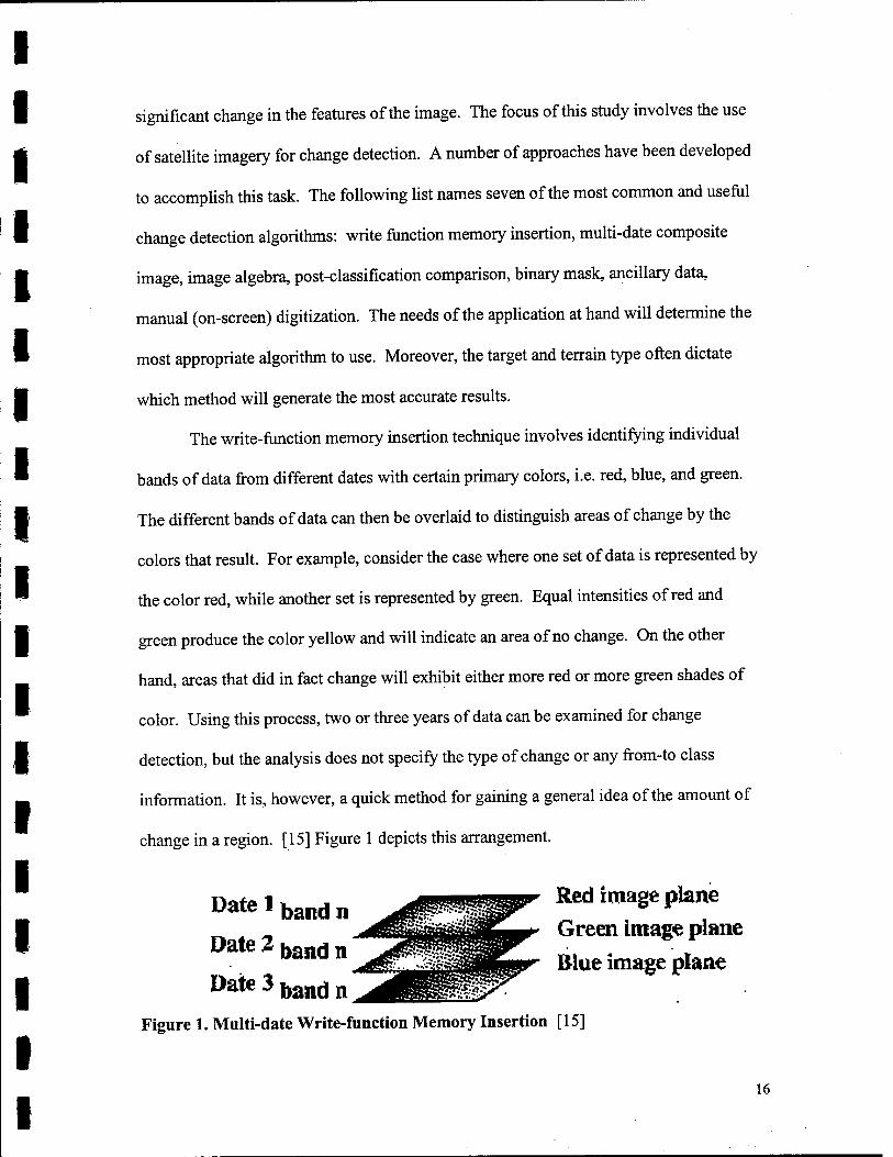
The write-function memory insertion technique involves identifying individual
bands of data from different dates with certain primary colors, i.e. red, blue, and green.
The different bands of data can then be overlaid to distinguish areas of change by the
colors that result. For example, consider the case where one set of data is represented by
the color red, while another set is represented by green. Equal intensities of red and
green produce the color yellow and will indicate an area of no change. On the other
hand, areas that did in fact change will exhibit either more red or more green shades of
color. Using this process, two or three years of data can be examined for change
detection, but the analysis does not specify the type of change or any from-to class
information. It is, however, a quick method for gaining a general idea of the amount of
change in a region. [15] Figure 1 depicts this arrangement.
Date IK H ,dpi§«r ft"! image plane ^^^^j» Green image plane
Date 2 band n ^^^^^^ „, . t ^rf^^ffipaapfcpr- Blue image plane
Figure 1. Multi-date Write-function Memory Insertion [15]
16
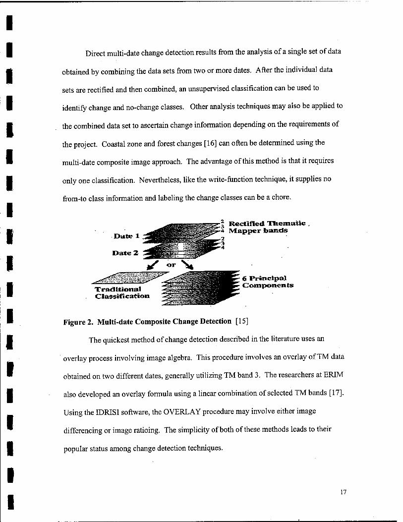
Direct multi-date change detection results from the analysis of a single set of data
obtained by combining the data sets from two or more dates. After the individual data
sets are rectified and then combined, an unsupervised classification can be used to
identify change and no-change classes. Other analysis techniques may also be applied to
the combined data set to ascertain change information depending on the requirements of
the project. Coastal zone and forest changes [16] can often be determined using the
multi-date composite image approach. The advantage of this method is that it requires
only one classification. Nevertheless, like the write-fünction technique, it supplies no
from-to class information and labeling the change classes can be a chore.
;| Rectified Thematic -4 Mapper bands
Traditional Cl assifi cation
6 Principal Componen ts
Figure 2. Multi-date Composite Change Detection [15]
The quickest method of change detection described in the literature uses an
overlay process involving image algebra. This procedure involves an overlay of TM data
obtained on two different dates, generally utilizing TM band 3. The researchers at ERIM
also developed an overlay formula using a linear combination of selected TM bands [17].
Using the IDRISI software, the OVERLAY procedure may involve either image
differencing or image ratioing. The simplicity of both of these methods leads to their
popular status among change detection techniques.
17
Image differencing relies upon the differences between corresponding pixel
values to indicate areas of change. Large values that result from calculating the absolute
value of the difference between corresponding pixels point to regions of change. When
graphed, the pixel values displaying significant change should lie in the tails of the
distribution, while all other values group around the mean [16]. Image differencing can
be applied to both single and multiple bands of data. However, if necessary, radiometric
corrections must be applied to the images before using the differencing technique. Land
erosion, deforestation, and urban growth provide examples of subjects that lend
themselves nicely to image differencing change detection.
Determining an appropriate difference map threshold embodies the true challenge
of image differencing. A difference map threshold is a pre-determined value or range of
values that measure whether the calculated difference in pixels indicates a change or no
change. When choosing the threshold value the analyst must consider factors, such as
fluctuating camera levels and viewing conditions, that may affect the outcome of the
differencing. If the threshold is too low, the results of the change detection will be
plagued by spurious changes. Likewise, an excessively high value may suppress
significant changes. Therefore, choosing a threshold is a critical task when using image
differencing.
Image ratioing resembles the differencing technique in its general simplicity;
however, this technique calculates a ratio of the values of corresponding pixels from
different images. If no significant change has occurred between two pixels, their values
should be similar and the ratio will be approximately equal to one. If significant change
has occurred, the ratio will be either much larger or much less than one. The advantage
18
of this technique is that, regardless of scene illumination variations, the image of ratios
will still convey spectral or color characteristics of the features in the image. However,
Lillesand and Kiefer caution the analyst to remember that images produced by ratioing
are "intensity blind." This means that materials that actually have distinct absolute
radiances may appear similar if the ratio of their spectral values is similar—this occurs
when the slope of their spectral reflectance curves are alike. [12] Therefore, as with all of
the techniques described here, care must be taken to avoid making unfounded
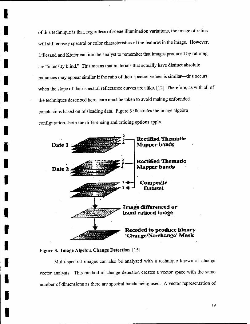
conclusions based on misleading data. Figure 3 illustrates the image algebra
configuration-both the differencing and ratioing options apply.
Date 1
Date 2
Rectified Thematic Mapper bands
Rectified Thematic Mapper bands
Composite Dataret
Image differenced or band ratfoed image
Recoded to produce binary 'Changc/No-change' Mask
Figure 3. Image Algebra Change Detection [15]
Multi-spectral images can also be analyzed with a technique known as change
vector analysis. This method of change detection creates a vector space with the same
number of dimensions as there are spectral bands being used. A vector representation of
19
each pixel can then be created using the brightness values of the pixels in each spectral
dimension as their coordinates. If a pixel changes between the first and second image,
the spectral change vector can be found by subtracting the two vectors that represent the
pixel at the two times [18]. This technique allows for the calculation of both the
magnitude and the direction of the change vector. However, the direction can only be
determined if two spectral bands are involved in the analysis. Like image algebra, this
technique also requires the determination of a threshold for the magnitude of the
calculated change vector in order to define whether change has or has not occurred.
Change detection using the post-classification technique requires the classification
of each image that will be used in the analysis. After classifying each image
independently, a comparison can be made either visually or using a computer to identify
areas of significant change. Visual interpretation may reduce registration errors since the
human eye can discriminate patterns and shapes; however, a computer may provide a
better quantitative analysis [16]. The analyst must decide which method best fits the
given study. The overriding disadvantage of this method is the possibility of
compounded errors due to multiple classifications. Any misclassification that occurs in
the preliminary classifications will be compounded with subsequent applications. In fact,
the overall accuracy can be calculated by multiplying the accuracy of each individual
classified image. The advantage of making individual classifications, however, is that the
analysis provides from-to class information. Examples of post-classification analysis
applications include urban changes, forest to crop land changes, and general land use
changes.
20
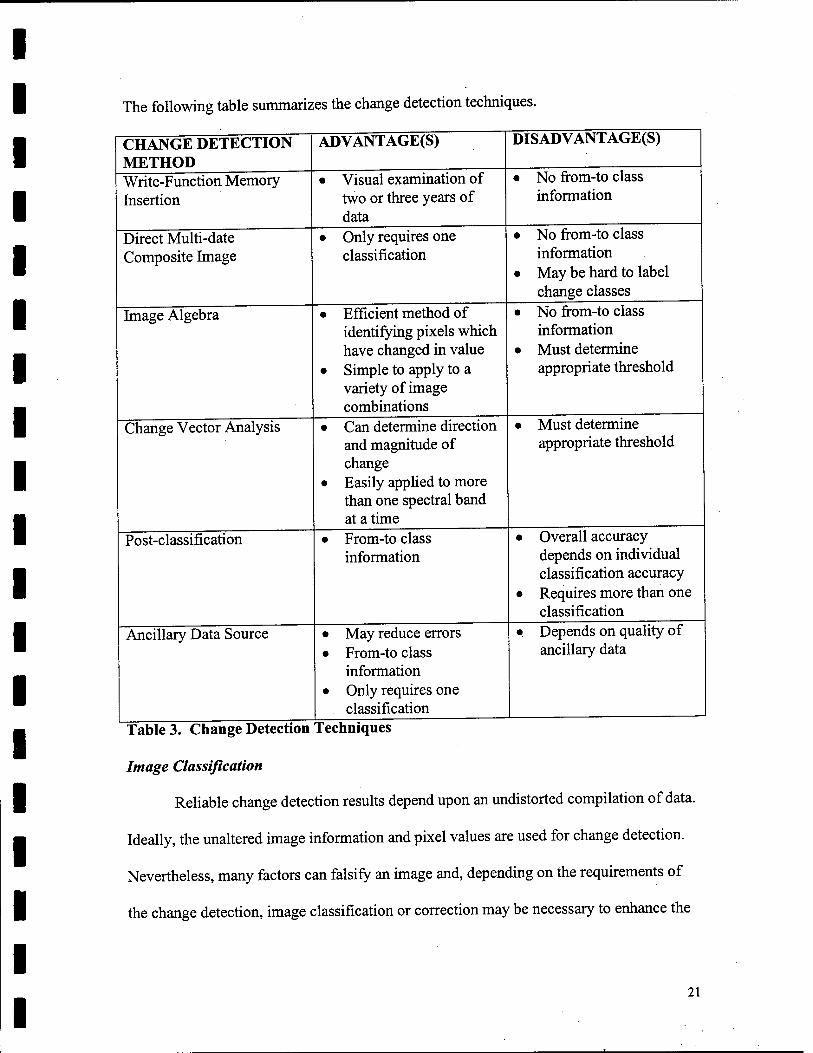
The following table summarizes the change detection techniques.
CHANGE DETECTION METHOD Write-Function Memory Insertion
Direct Multi-date Composite Image
Image Algebra
Change Vector Analysis
Post-classification
Ancillary Data Source
ADVANTAGE(S)
Visual examination of two or three years of data Only requires one classification
Efficient method of identifying pixels which have changed in value Simple to apply to a variety of image combinations
• Can determine direction and magnitude of change
• Easily applied to more than one spectral band at a time
DISADVANTAGE(S)
No from-to class information
• No from-to class information
• May be hard to label change classes
• No from-to class information
• Must determine appropriate threshold
From-to class information
• May reduce errors • From-to class
information • Only requires one
classification
• Must determine appropriate threshold
Overall accuracy depends on individual classification accuracy Requires more than one classification
• Depends on quality of ancillary data
Table 3. Change Detection Techniques
Image Classification
Reliable change detection results depend upon an undistorted compilation of data.
Ideally, the unaltered image information and pixel values are used for change detection.
Nevertheless, many factors can falsify an image and, depending on the requirements of
the change detection, image classification or correction may be necessary to enhance the
21
original data to create the change detection database. The goal of image classification is
to employ any algorithm or collateral data, such as DEM's or soil maps, to improve the
accuracy of the image [15]. There are two main types of image classification that will be
described in further detail: supervised and unsupervised.
Supervised classification involves a training stage, when the analyst "trains" the
classifier by supplying the criteria necessary for pixels from a single date to belong to
known phenomena. A minimum-distance-to-means algorithm then places the pixels in
their appropriate category and assigns unknown pixels to the nearest class or the class to
which they have the highest probability of belonging. The training stage is of supreme
importance because it is the building block of the classification and ultimately the change
detection process. If the classified data are faulty, the change detection will also be
incorrect.
Unsupervised classification relies upon the computer to inspect the data and
identify a specified number of mutually exclusive clusters—groups of pixels that appear
to exhibit the same spectral characteristics. Then, the analyst is left to determine the
classes to which those clusters belong based on ancillary data or ground truth. This
method of classification generally produces less accurate classifications than the
supervised method; however, some studies may not have enough preliminary
information to perform a supervised classification.
Quality Assurance
As with most scientific analyses, accuracy assessments often supplement remote
sensing investigations to account for and analyze sources of error. To produce an
accuracy assessment for a remote sensing application, the procedure generally requires
22
obtaining a "source of higher accuracy" [15] other than the remotely sensed images.
Examples of sources include higher resolution photographs, verified field maps, or
ground truth. Due to the inherent nature of change detection, accuracy assessments can
often be impractical or unfeasible. Change detection usually involves images acquired
over a length of time and, thus, actual field verification is often unavailable for past dates.
Nevertheless, several quality assurance gauges will be described below since they may be
applicable to change detection projects under the correct circumstances. Each of these
accuracy measures is discussed in the C-CAP manual, along with others.
Lineage refers to the type of data sources used in the analysis and the operations
involved in creating the database. As previously mentioned, the resolutions of the images
and the dates of the materials should coincide. Using the same source of information and
sensor type generally provides the easiest way to create these necessary conditions and
reduce errors caused by lineage differences.
The completeness of an analysis refers to the extent to which the data addresses
all possible combinations and conclusions. Classification data, for example, should
include all categories present in the image. Furthermore, every pixel in an image should
be assigned to one of the classes. Any missing data can potentially alter the results of a
change detection analysis due to a lack of completeness.
The fitness for use gauge measures the degree to which the image and ancillary
data actually relate to the application at hand. One of the first tasks before beginning any
analysis requires that the data be assessed for its applicability to the study. Although a
set of data may provide results, the results might not address the matter of concern and
therefore are not fit for use.
23
Attribute accuracy estimates the probability that the land cover types given to
each class in the image properly identify the actual land cover. According to the C-CAP
manual, this accuracy measurement works best for studies involving current time periods
and relatively small areas. The reason for these stipulations relates back to the earlier
discussion of the applicability of accuracy measurements to change detection analyses in
general. (Field verification cannot usually be obtained and large areas demand extensive,
in-depth verification to be accurate.) Specifically, "accuracy assessments of large change
databases are infeasible due to the combination of past time periods, large areas, and
excessive from-to classes" [15]. Hence, when accuracy assessments prove to be
impractical, the objective should be to strive for consistency of technique more than
accuracy.
ANALYSIS
Objective
The aim of this investigation is to identify areas of significant change along
Fountain Creek using satellite imagery and remote sensing methodology. For the
purposes of this analysis, areas of significant change are areas where satellite sensors
detect large differences in electromagnetic energy, resulting in large deviations in pixel
values over time. The deliverables of the analysis will consist of images that offer a
visual representation of the changes along Fountain Creek and in the surrounding study
area.
The study area spans a stretch of Fountain Creek located just south of the
metropolitan Colorado Springs area, to the west of the Colorado Springs airport, and to
24
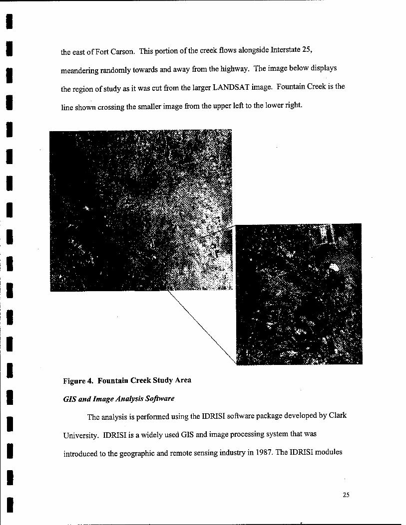
the east of Fort Carson. This portion of the creek flows alongside Interstate 25,
meandering randomly towards and away from the highway. The image below displays
the region of study as it was cut from the larger LANDS AT image. Fountain Creek is the
line shown crossing the smaller image from the upper left to the lower right.
Figure 4. Fountain Creek Study Area
GIS and Image Analysis Software
The analysis is performed using the IDRISI software package developed by Clark
University. IDRISI is a widely used GIS and image processing system that was
introduced to the geographic and remote sensing industry in 1987. The IDRISI modules
25
utilized to register the images and perform the calculations include: WINDOW,
COMPOSIT, CONCAT, OVERLAY, HISTO, SCALAR, RECLASS, and TRANSFOR.
These modules permit a variety of image processing techniques, two of which will be
presented here: image differencing and change vector analysis.
Available Data
Thematic Mapper imagery is collected regularly by LANDSAT satellites and
provides a convenient source of data to detect changes over large areas. The following
list describes the digital satellite imagery from LANDSAT that was used for the Fountain
Creek analysis:
• Three sets of LANDSAT TM data including files for all seven spectral bands- blue, green, red, near infrared, two mid-infrared, and one thermal infrared--for each image.
• First Set: April 1993 • Second Set: 4 July 1994 • Third Set: 26 June 1997 • The LANDSAT 5 (L5) satellite acquired each image.
A USGS map of the Colorado Springs area was also used to locate landmark sites
to help verify the location of Fountain Creek and to gain a perspective for resizing the
images for analysis.
Expected Results
Based on past research of the Fountain Creek region and the written and visual
information provided by the Fountain Creek Watershed Project and the United States
Geological Survey, significant areas of change should be visible along Fountain Creek.
Case studies suggest that certain stretches of land along the creek demonstrate more
vulnerability to erosion than others and, in fact, have the potential to change drastically
overnight. The most vulnerable regions should therefore exhibit the most visible changes
26
in the change detection process and, because the analysis utilizes differences in raw pixel
values, those areas should provide the best opportunity for accurate change assessments.
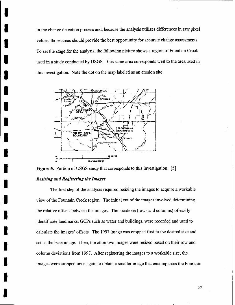
To set the stage for the analysis, the following picture shows a region of Fountain Creek
used in a study conducted by USGS—this same area corresponds well to the area used in
this investigation. Note the dot on the map labeled as an erosion site.
COLORADO
|«>'S«3s.,\. fi J5?Y / //f_
Js r
\ -I
5 _j 1_
19 <it>vf Trnr:
Figure 5. Portion of USGS study that corresponds to this investigation. [5]
Resizing and Registering the Images
The first step of the analysis required resizing the images to acquire a workable
view of the Fountain Creek region. The initial cut of the images involved determining
the relative offsets between the images. The locations (rows and columns) of easily
identifiable landmarks, GCPs such as water and buildings, were recorded and used to
calculate the images' offsets. The 1997 image was cropped first to the desired size and
set as the base image. Then, the other two images were resized based on their row and
column deviations from 1997. After registering the images to a workable size, the
images were cropped once again to obtain a smaller image that encompasses the Fountain
27
Creek region of interest. The selected area provides a region where the creek can be
easily distinguished from its surroundings (See Figure 4).
Ideally, no more than a VA to Vi pixel offset should exist between registered images
for accurate results. Therefore, to ensure that the images were registered with minimal
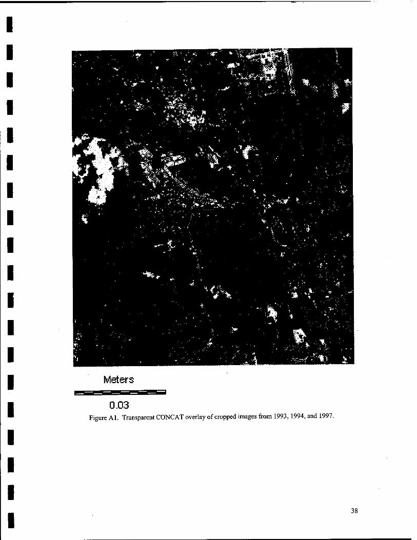
pixel offsets, the CONCAT function was used to overlay the images as if they were
transparencies. The resulting image, shown in Appendix A, provides a visual
representation of the deviations in the original images. The CONCAT image shows
minimal distortion, with clearly visible landscape features, indicating that the cropped
images correspond well. If the images did not correspond, the CONCAT image would
have appeared more skewed and distorted.
The image enhancement and image correction capabilities of IDRISI were also
explored, using the RADIANCE and RESAMPLE modules, respectively, but the altered
images were not used in the analysis for several reasons. First, the resource that discusses
the radiance correction module gives a very brief description of its use, with no reference
to the actual calculations performed. Furthermore, the descriptive information provided
with the images affirms that the images were acquired with similar sun angles, reducing
the effects of sun angle variations. Above all, however, the desire to maintain the
original pixel values for the calculations in order to avoid altering the data and skewing
the results drove the decision to use the raw images.
Differencing with Composite Images
The first set of difference images was created using a combination of three
corresponding spectral bands from each date. The combination of bands enhances the
visibility of the creek without altering the pixel values. Three different composite images
28
for each date were created using the COMPOSIT module. The first composite set
involves bands 3,4, and 5. The IDRISI handbook suggests using this combination of
bands for any general analysis. The second composite image involves bands 4, 5, and 7,
and the third combination is made up of bands 3, 5, and 7. All of the composite
combinations correspond to the blue, green, and red bands, in that order.
One reason for choosing the given combinations is that water strongly absorbs
infrared wavelengths making it highly distinguishable in that region. The infrared bands
therefore highlight the creek since its water reflects less light than the surrounding soil,
vegetation, and concrete. It should be noted however that extra sediment in the water on
any given date reflects more light than clear water. Also, the turbidity of the water
affects the water's reflectance properties. Furthermore, while LANDSAT TM Band 5 is
placed between two water absorption bands making it very useful in determining soil
moisture differences, the calculated changes may be based on soil moisture rather than
actual differences in landscape due to erosion. Thus, while the band combinations were
chosen for their beneficial characteristics, the potential sources of error that they present
must not be overlooked. For further clarification of the combination choices, refer back
to Table 2.
Once the composite images were created, the OVERLAY module was used to
perform the image differencing. Difference images were created for each pair of dates—
1997/1994,1994/1993,1997/1993 (subtracting the earlier date from the later date)—with
all three composite combinations. A histogram of each difference image was created
using the HISTO module to display the spread of pixel values that resulted from the
differencing procedure. For each of the images, the pixel values generally spread from
29
-215 to +215. Then, for display purposes, the SCALAR module was used to generate all
positive DNs. This module simply adds a specified integer value to each of the original
DNs. The final difference images, displayed with the gray 256 palette, and several of
their corresponding histograms are shown in Appendix B. Note that the histograms for
the composite images show several peaks in the data distribution, but the overall shape
resembles a normal distribution around the mean. The various peaks are believed to be a
result of using more than one band of data.
At this point in the study, the gray scale images display the areas of change based
on the relative values of the pixels. The highest DNs correspond to the lightest areas in
the image. These areas signify that the values from the earlier date were relatively small
compared to the later date's values. Likewise, regions with the lowest DNs correspond to
the darkest areas in the image, and indicate that the pixel values on the earlier image were
much higher than the values on the later image in that region.
The next step was to calculate threshold values for the change in each image.
There are no distinct guidelines for selecting threshold values, however image histograms
are often used as an aid. The histograms provide statistical data about the images such as
the mean and standard deviation of the pixel values. While the needs of each application
may vary, one standard deviation is generally considered to be a reasonable threshold for
determining positive, negative, and no change conditions. As such, the threshold values
used in this study were one standard deviation on either side of the mean.
With the threshold values determined, the RECLASS module was used to create
images that display the three levels of change. A value of zero was assigned to all DNs
in the difference images that were within one standard deviation of the mean. This means
30
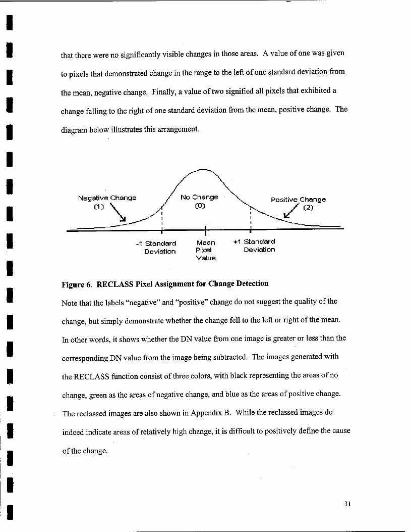
that there were no significantly visible changes in those areas. A value of one was given
to pixels that demonstrated change in the range to the left of one standard deviation from
the mean, negative change. Finally, a value of two signified all pixels that exhibited a
change falling to the right of one standard deviation from the mean, positive change. The
diagram below illustrates this arrangement.
Negative Change Positive Change
7™ -1 Standard
Deviation Mean Pixel Value
1-1 Standard Deviation
Figure 6. RECLASS Pixel Assignment for Change Detection
Note that the labels "negative" and "positive" change do not suggest the quality of the
change, but simply demonstrate whether the change fell to the left or right of the mean.
In other words, it shows whether the DN value from one image is greater or less than the
corresponding DN value from the image being subtracted. The images generated with
the RECLASS function consist of three colors, with black representing the areas of no
change, green as the areas of negative change, and blue as the areas of positive change.
The reclassed images are also shown in Appendix B. While the reclassed images do
indeed indicate areas of relatively high change, it is difficult to positively define the cause
of the change.
31
Single Band Image Differencing
Single band difference images were also created to compare to the composite
difference images. Bands 5 and 7 were used to create individual band difference images
between the three dates. The same steps as described for the composite images—using
the OVERLAY, WINDOW, HISTO, SCALAR, and RECLASS modules—were used,
but with only one band from each date instead of three. The single band difference
images and their histograms are given in Appendix C. Like the histograms for the
composite images, the histograms for the single band images take on the shape of a
normal distribution about the mean. However, for the single band difference images,
there are only single peaks in the data distributions—likely the result of comparing only
one band.
The single band difference images can be interpreted the same as the composite
images. No new information is revealed in these images, but they do provide a broken
down view of the changes by spectral band.
Change Vector Analysis
Change vector images were created using two bands—Bands 5 and 7—from each
date. First, the single band difference images were squared using the TRANSFOR
function, working with only two of the dates at a time. Those images were then added
using OVERLAY. The final image resulted from taking the square root of the image sum
using the TRANSFOR function once again. See the change vector images in Appendix
D. The colors in the change vector images—displayed using the Idrisi 256 palette-
represent the magnitude of the change vector. Dark blacks and blues signify areas of low
32
I I
change. Shades of red show intermediate change, and yellows and greens indicate areas
with a high magnitude of change.
Discussion of Images
The main area of concern for this investigation is the creek that flows diagonally
from upper left to lower right in the images. While inferences can be made about other
areas appearing in the images, they will not be addressed here. Also note that the clouds
in the 1997 image, which appear on the left side of the images involving 1997 in the
calculations, must not be considered in the analysis. In addition, due to the many factors
that can skew the results of a purely mathematical analysis, many of the inferences made
from the images result from a purely visual comparison and interpretation.
The images created with the differencing procedure do indeed display the
expected change along Fountain Creek and expose areas that demonstrate the greatest
relative change. The light and dark shades in the gray scale images indicate the degree to
which regions of the creek have changed according to raw pixel values. The reclassed
images, on the other hand, provide a more clear cut representation of the areas that
demonstrate the greatest probability to have changed and the general direction of the
change, i.e. whether the smaller DN came from the earlier date or the later date. Smaller
DNs could be the result of wetter soil since water reflects less in the infrared. Hence, if
the smaller DN came from the earlier date—resulting in positive change-the soil could
have become drier as the creek cut further into the land and away from the area,
increasing the DN value on the later date. On the other hand, if the smaller DN came
from the later date—resulting in a negative change—the creek may have eroded the land
and started to flow over it. Nevertheless, the exact cause of the detected change is
33
uncertain due to the many factors detailed throughout the paper that affect pixel values.
The suggestions presented here offer just one possible interpretation.
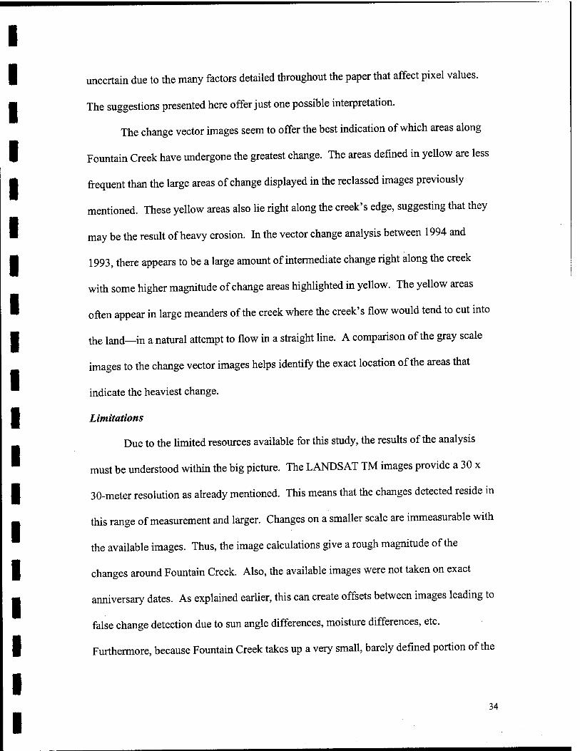
The change vector images seem to offer the best indication of which areas along
Fountain Creek have undergone the greatest change. The areas defined in yellow are less
frequent than the large areas of change displayed in the reclassed images previously
mentioned. These yellow areas also lie right along the creek's edge, suggesting that they
may be the result of heavy erosion. In the vector change analysis between 1994 and
1993, there appears to be a large amount of intermediate change right along the creek
with some higher magnitude of change areas highlighted in yellow. The yellow areas
often appear in large meanders of the creek where the creek's flow would tend to cut into
the land—in a natural attempt to flow in a straight line. A comparison of the gray scale
images to the change vector images helps identify the exact location of the areas that
indicate the heaviest change.
Limitations
Due to the limited resources available for this study, the results of the analysis
must be understood within the big picture. The LANDSAT TM images provide a 30 x
30-meter resolution as already mentioned. This means that the changes detected reside in
this range of measurement and larger. Changes on a smaller scale are immeasurable with
the available images. Thus, the image calculations give a rough magnitude of the
changes around Fountain Creek. Also, the available images were not taken on exact
anniversary dates. As explained earlier, this can create offsets between images leading to
false change detection due to sun angle differences, moisture differences, etc.
Furthermore, because Fountain Creek takes up a very small, barely defined portion of the
34
raw images provided by LANDS AT, the images were cropped to facilitate the analysis of
the specified region. The locations of major landmarks in the three sets of images did not
correspond pixel for pixel. Hence, the cropping procedure involved cutting the images to
the closest pixel to pixel correspondence possible. This means that error may have been
introduced in the image registration process if the pixels from each date do not perfectly
coincide. Much care was taken to ensure the best fit; however, more care must be taken
not to overlook this possible source of error.
With a more in-depth analysis of the geography and ground cover of the region,
these images may help verify which zones along the creek demonstrate more
vulnerability to erosion. Unfortunately, digital elevation models were unavailable to
perform a change analysis on the elevations in the area. This type of analysis would help
verify if the changes detected in the spectral analysis are due to changes in ground
elevation caused by erosion or whether other factors affected the results of the change
analysis. Furthermore, the many external factors that influence the image processing
calculations complicate the calculation of reliable figures to describe the changes along
Fountain Creek. In addition, because the changes along Fountain Creek could potentially
go undetected within the resolution of LANDS AT TM imagery, a more specific
quantitative analysis of the change would be counterproductive. However, while aerial
photography, which can also be used for remote sensing analyses, is less convenient to
use, is not collected on a regular basis, and is more costly, it may provide the means to
perform a more quantitative analysis in the future.
35
CONCLUSION
Satellite remote sensing and GIS technology are the key to gaining a keener
insight into the erosive processes at work on the Earth's surface. Analyses that are
committed to taking full advantage of the enhanced satellite and GIS technology can help
explain how human activities throw the Earth's natural processes out of balance.
Moreover, a better understanding of erosion may aid in the careful placement of new
pavement and buildings as well as improve the current resource management procedures.
This could ultimately lead to a fewer number of dilemmas in the future.
This investigation in particular was performed as a part of a research proposal
submitted to NASA for the study of the erosion and pollution problems of the Fountain
Creek Watershed. The images presented in the analysis provide a visual representation of
the areas that display the greatest change. Although the results of this study do not
provide solutions to the erosion problem, the information provided and the images
generated act as a stepping stone to support further studies of the area.
36
APPENDIX A
TRANSPARENT CONCAT IMAGE
37
Meters
0.03 Figure Al. Transparent CONCAT overlay of cropped images from 1993, 1994, and 1997.
38
APPENDIX B
COMPOSITE DIFFERENCE IMAGES
AND RECLASSED IMAGES
39
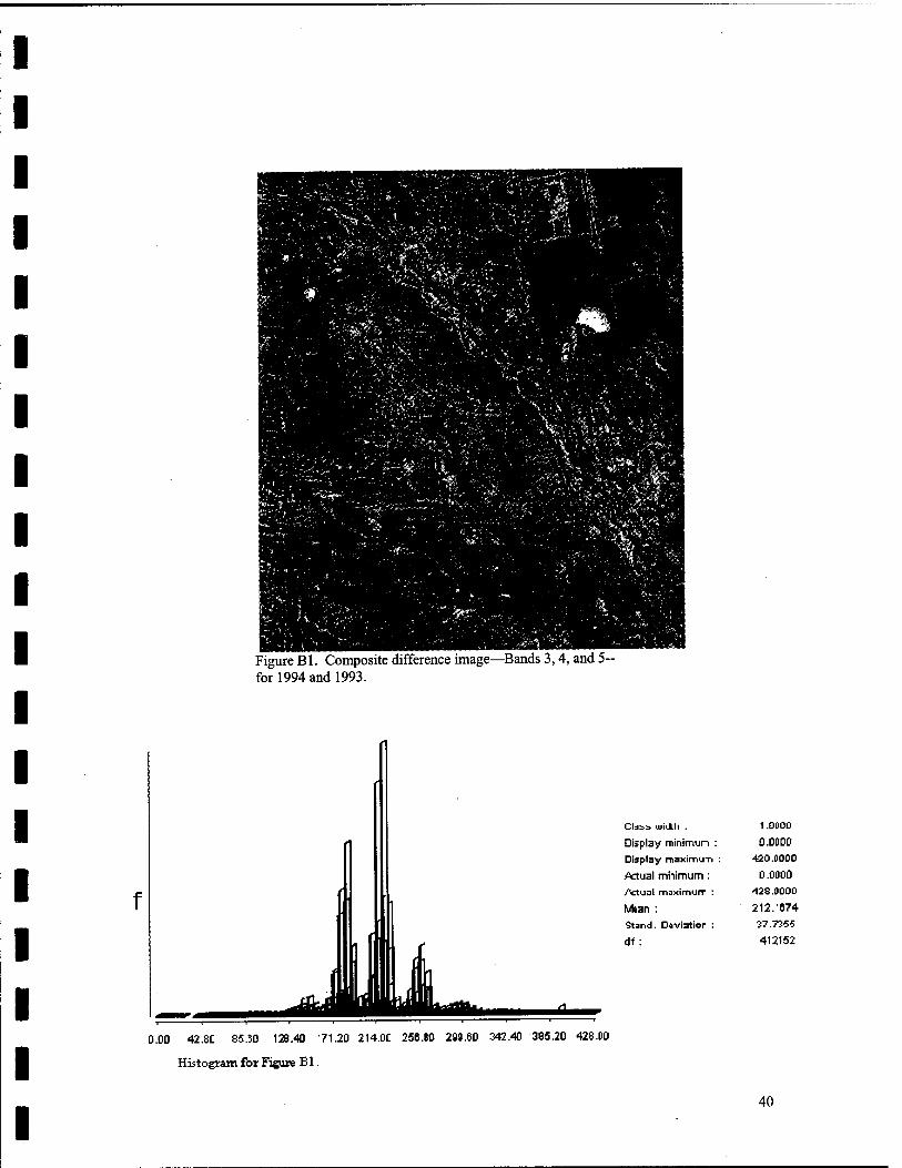
Figure Bl. Composite difference image—Bands 3,4, and 5- for 1994 and 1993.
f
O.DD 42.8C 85.30 128.40 71.20 214.0C 256.:
Histogram for Figure Bl.
299.60 342.40 385.20 428.00
CldiS UjiiJ.ll . 1.0000
Display minimun : 0.0000 Display maximu-n : 420.0000
A3ual mhimum : 0.0D00 /"ctual maximurr : 129.0000
Mean : 212.674 Stand. Deviatior : •27.7355
df : 412152
40
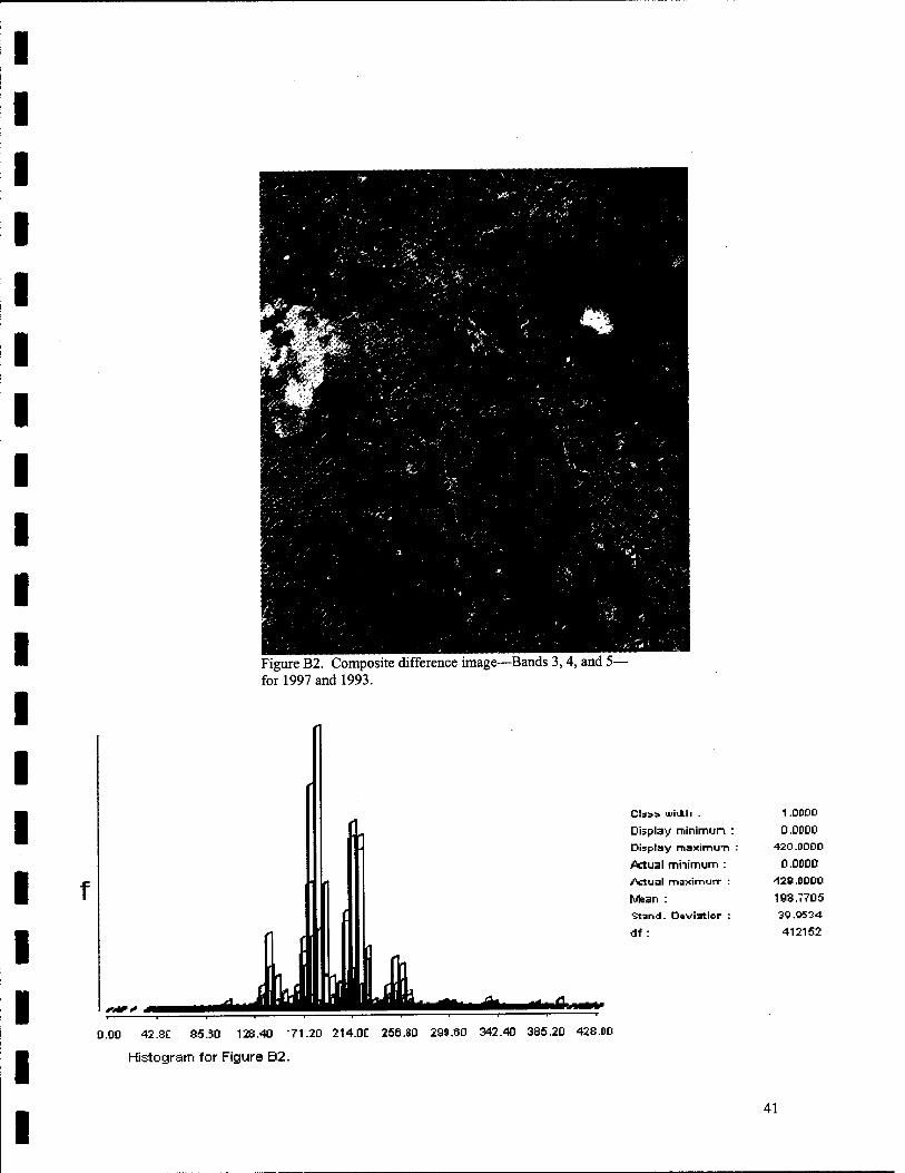
Figure B2. Composite difference image—Bands 3,4, and 5- for 1997 and 1993.
0.D0 42.8C 85.30 128.40 71.20 214.0C 256.80 299.80 342.40 385.20 428.00
Histogram for Figure B2.
CldiS uuiij.ll . 1.0000
Display minimun : 0.0Ü00 Display maximuTi : 420 .DODO
actual mhimum : 0.0D00 /Vtual maximurr : 128.0000
Mean : 198.7705
Stand. O«viatior : 30. 0534
df : 412152
41
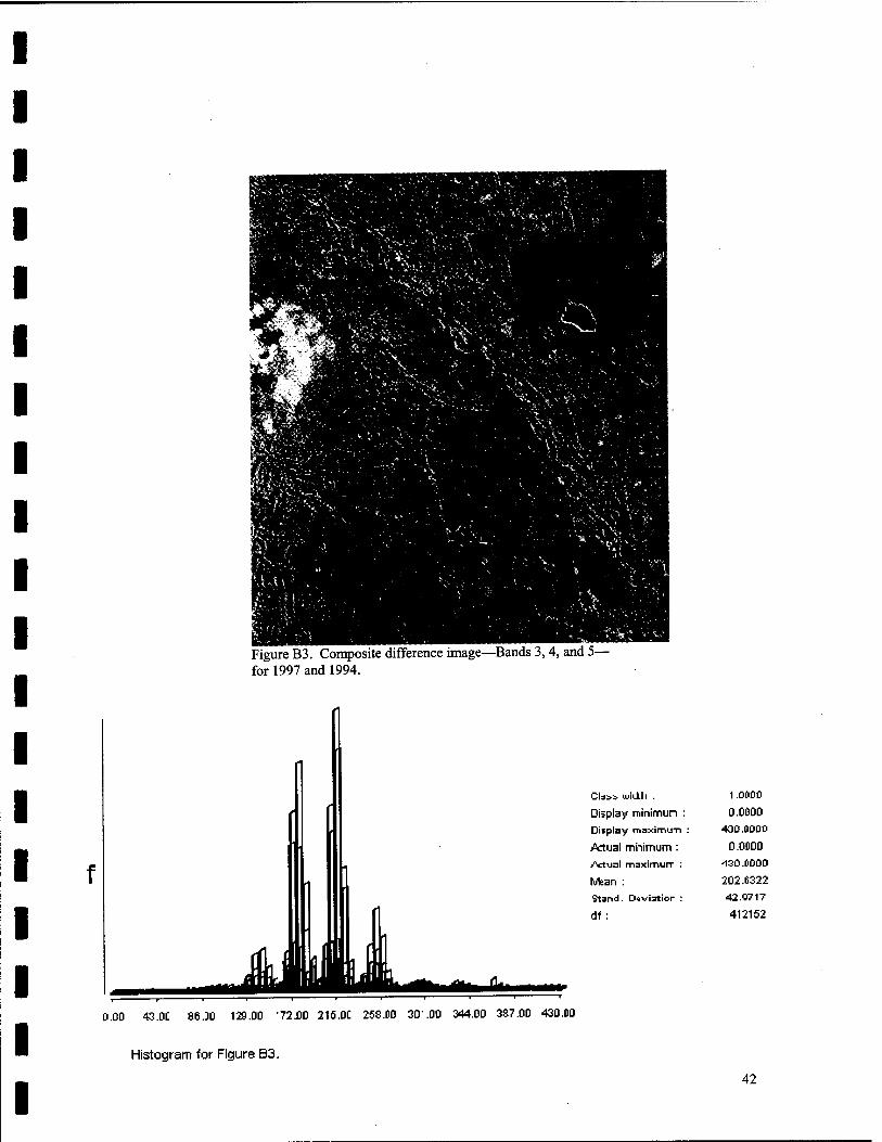
Figure B3. Composite difference image—Bands 3,4, and 5- for 1997 and 1994.
f
Clds-i wid.il . 1.0000
Display minimun : 0.DDD0
Display maximuTi : 400 .DODO
actual mhimum: O.D0OD
/actual maximurr : -130.0000
Mean : 202.6322
Stand. Dtviatior : 42.0717
df : 412152
D.DD 43.DC 86.30 129.Ü0 72.00 215.0C 258.D0 30".00 344.00 387.00 430.00
Histogram for Figure B3.
42
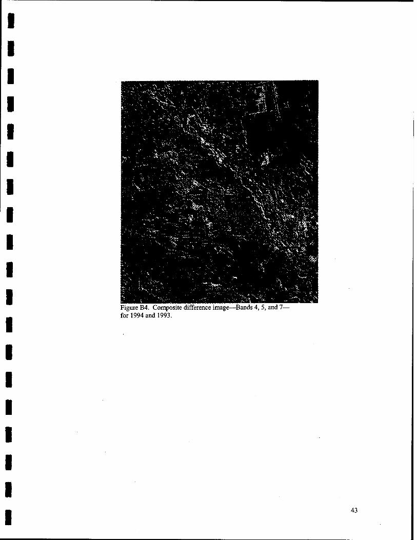
Figure B4. Composite difference image- for 1994 and 1993.
-Bands 4, 5, and 7—
43
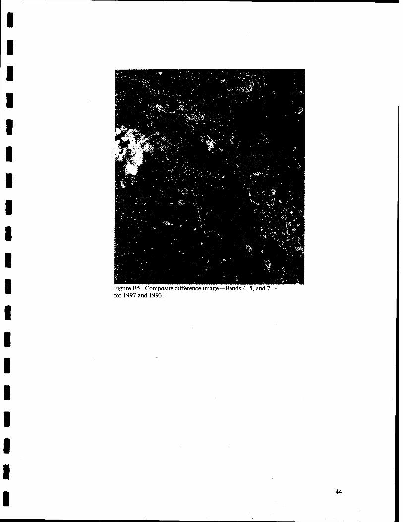
Figure B5. Composite difference image- for 1997 and 1993.
-Bands 4, 5, and 7-
44
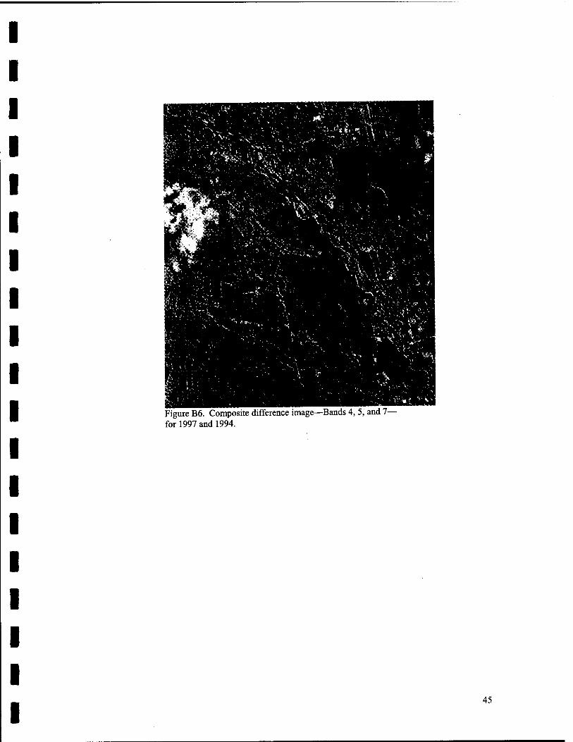
Figure B6. Composite difference image—Bands 4, 5, and 7— for 1997 and 1994.
45
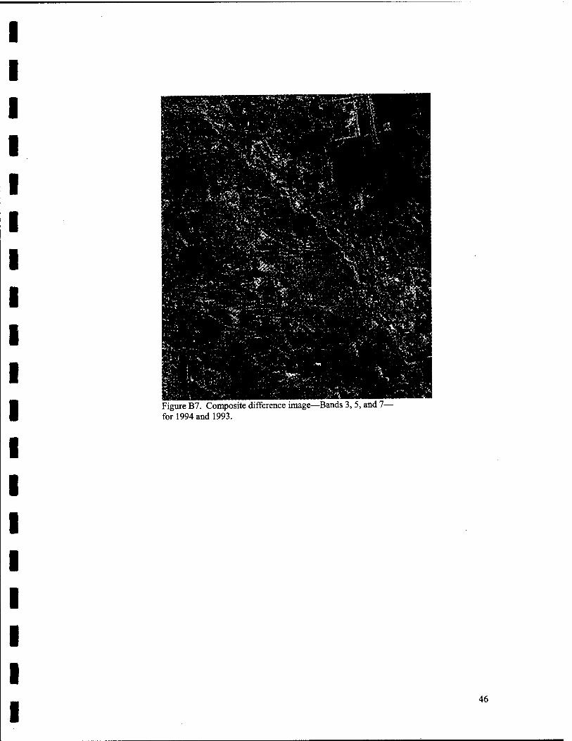
Figure B7. Composite difference image—Bands 3, 5, and 7— for 1994 and 1993.
46
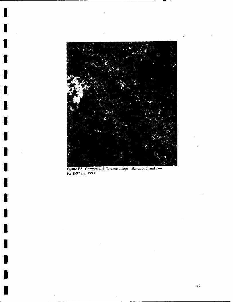
Figure B8. Composite difference image—Bands 3, 5, and 7— for 1997 and 1993.
47
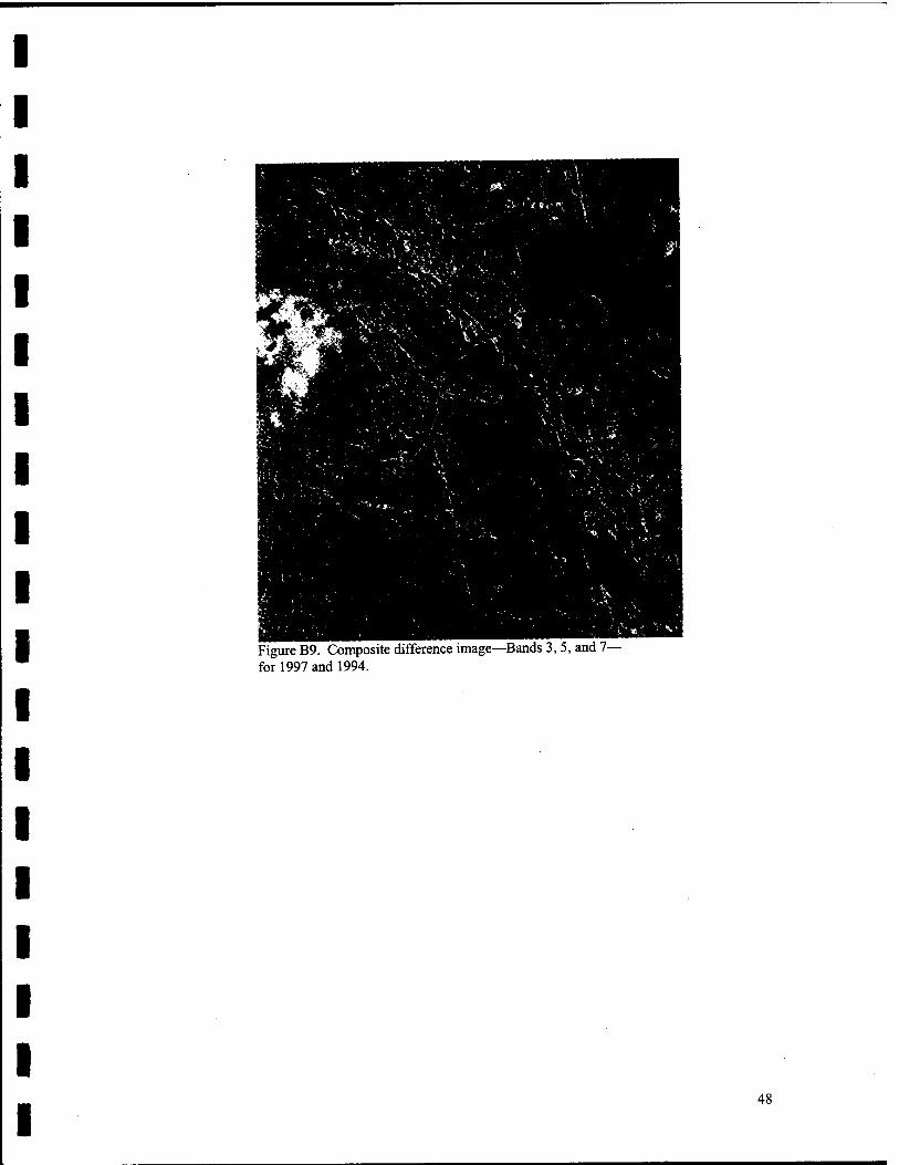
Figure B9. Composite difference image—Bands 3, 5, and 7— for 1997 and 1994.
48
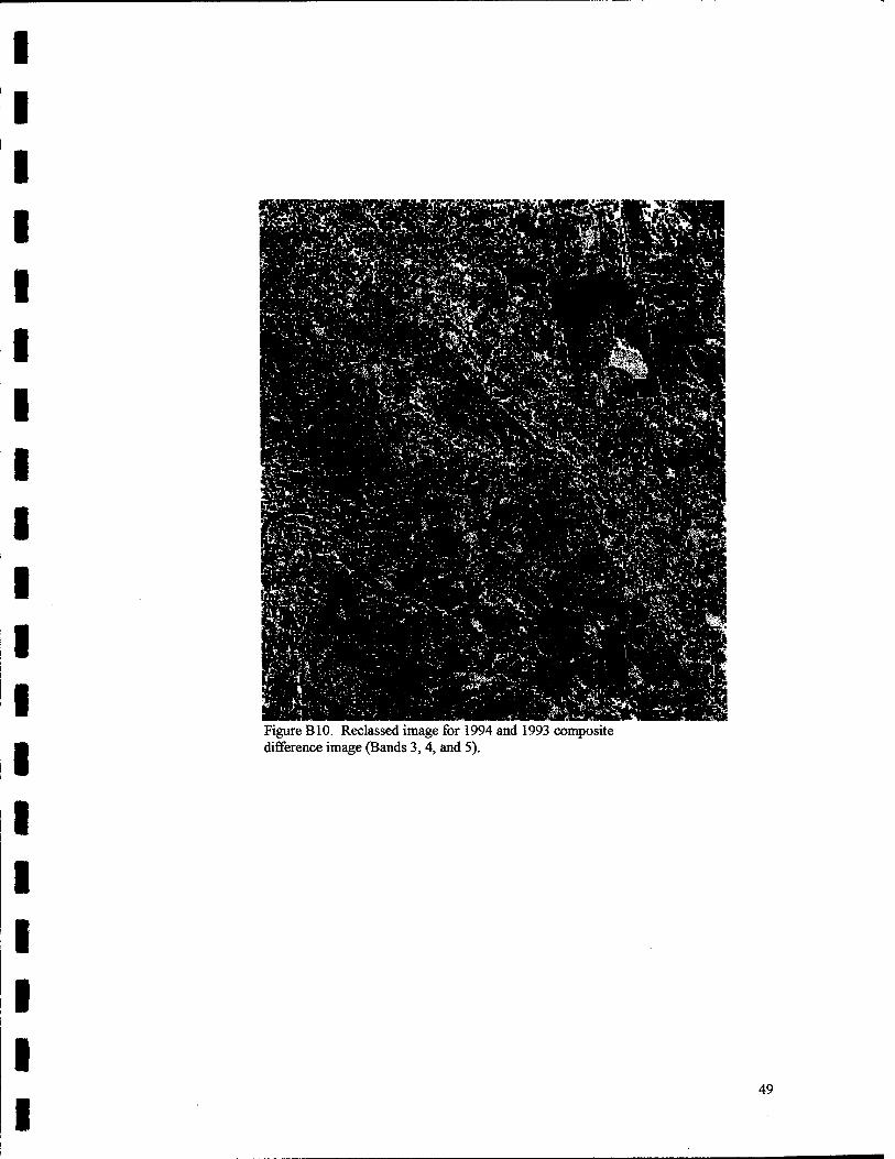
Figure BIO. Reclassed image for 1994 and 1993 composite difference image (Bands 3, 4, and 5).
49
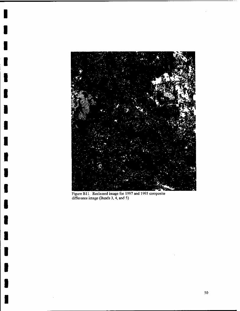
Figure Bll. Reclassed image for 1997 and 1993 composite difference image (Bands 3, 4, and 5)
50
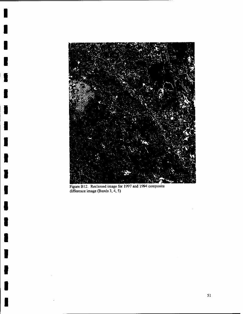
Figure B12. Reclassed image for 1997 and 1994 composite difference image (Bands 3, 4, 5)
51
APPENDIX C
SINGLE BAND DIFFERENCE IMAGES
AND THEIR HISTOGRAMS
52
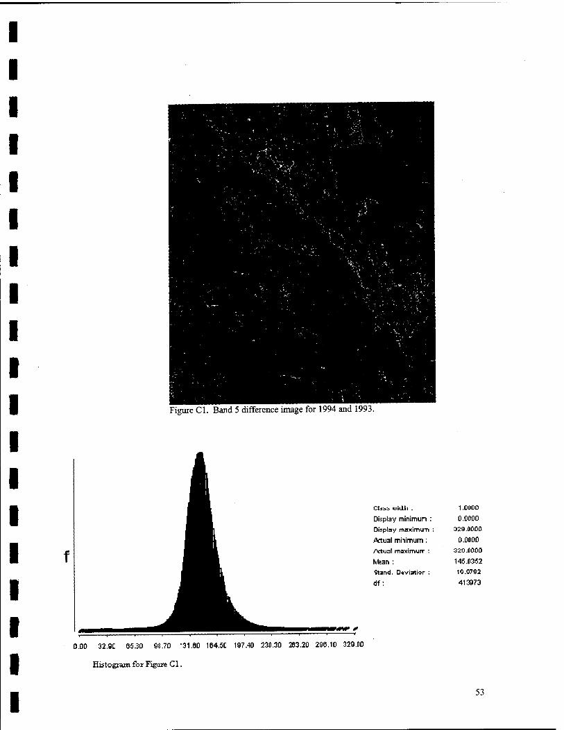
Figure Cl. Band 5 difference image for 1994 and 1993.
f
Cbii wiii.li . 1.0000
Display minimun : D.0D0D
Display maximu-n : 029.0000
.Actual minimum: D.ODDD
/actual maximurr : 320.0000
Mean : 145.0352
Stand. Dtviatior : 10.0782
df: 413973
D.0D 32.9t 65.30 98.70 "31.80 164.5C 197.40 230.30 263.20 296.10 329.00
Histogram for Figure Cl.
53
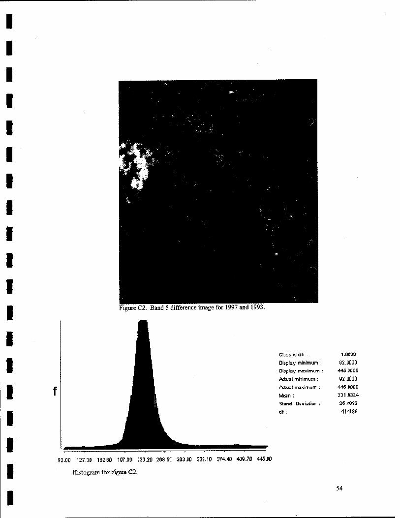
Figure C2. Band 5 difference image for 1997 and 1993.
f
Cldib wiU.ll . 1.0000
Display minimun : 92.0000
Display maximim : 445.0000
actual mhimum: 92.0000
/"ctual maxirnurr : 115.0000
Mian : 231.9334
Stand. Dtviatior : 25.««
df: 414189
92.00 127.30 162 60 197.90 233.20 268.5C 303.S0 339.10 374.40 409.70 445.00
Histogram for Figvure C2.
54
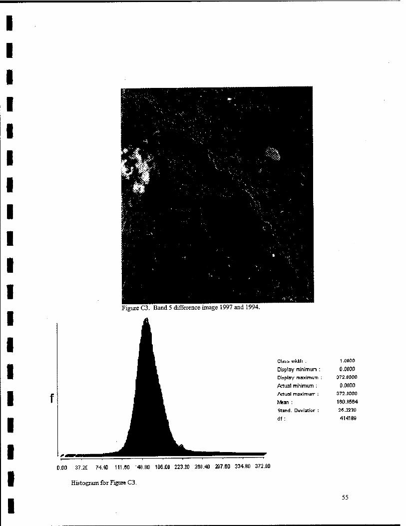
Figure C3. Band 5 difference image 1997 and 1994.
f
Cbsi luiilh . 1.0000
Display minimun : 0.0000
Display maximum : 072.0000
A^ual mhimum : 0.0D00
Actual maximurr : 372.0000
Mean : 160.8564
Stand. Daviatior : 25.22-30
df: 414189
D.ÜD 37.2C 74.40 111.60 '48.80 186.00 223.20 260.40 297.60 334.80 372.00
Histogram for Figure C3.
55
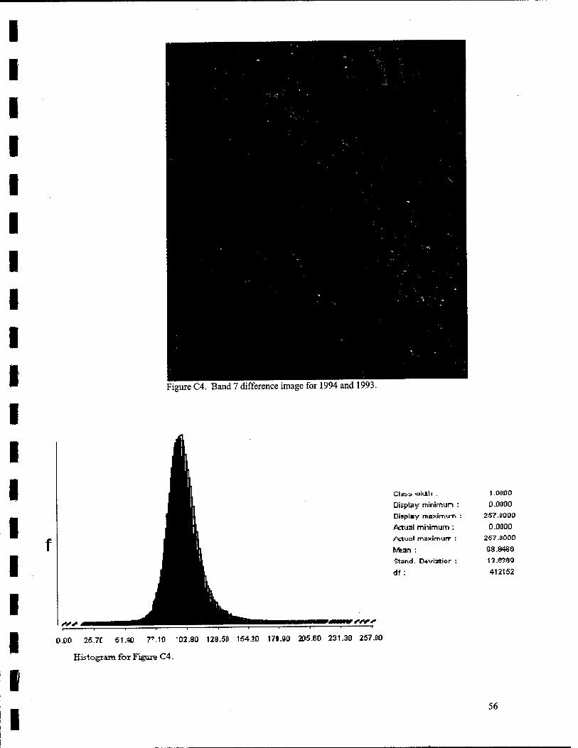
Figure C4. Band 7 difference image for 1994 and 1993.
0.00 25.7t SI.» 77.10 02.80 128.50 154.20 179.90 205.60 231.30 257.DO
Histogram for Figure C4.
I I
Cldi-i (JUiJ.il . 1 .DDDO
Display minimun : 0.0D00
Display maximuTi : 257.DODO
.Actual mhimum : 0.0D00
/actual maximurr : 267 .D000
Mean : 98.8486
Stand. D*viatior : 13.6580
df : 412152
56
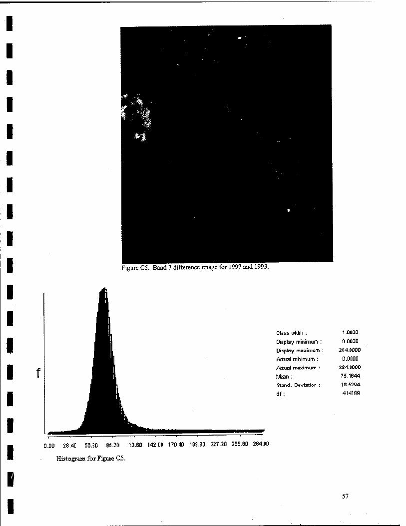
Figure C5. Band 7 difference image for 1997 and 1993.
f
0.00 28.4C 56.30 85.20 13.60 142.00 170.40 198.80 227.20 255.60 284.D0
Histogram for Figure C5.
CldS-i willll . 1 .D0OO
Display minimun : 0.0D00
Display maximuTi : 204.0000
Actual mhimum : 0.0D00
/■dual maximurr : 284.0000
Mean : 75.1644
Stand. Daviatior : 18.5204
df: 414189
57
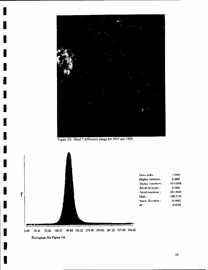
Figure C6. Band 7 difference image for 1997 and 1994.
f
CldiS Uliklll . 1 .DDOO
Display minimun : O.DDOD
Display maximum : 064.Ü0D0
actual mhimum: O.DDOD
.Actual maximurr : ae-UDoo
Mean : 146.3135
Stand. Daviatior : 10.6402
df : 414189
0.0D 36.4C 72.30 109.20 40.60 182.DC 218.40 25+.80 291.20 327.60 364.00
Histogram for Figure C6.
58
APPENDIX D
CHANGE VECTOR ANALYSIS IMAGES
59
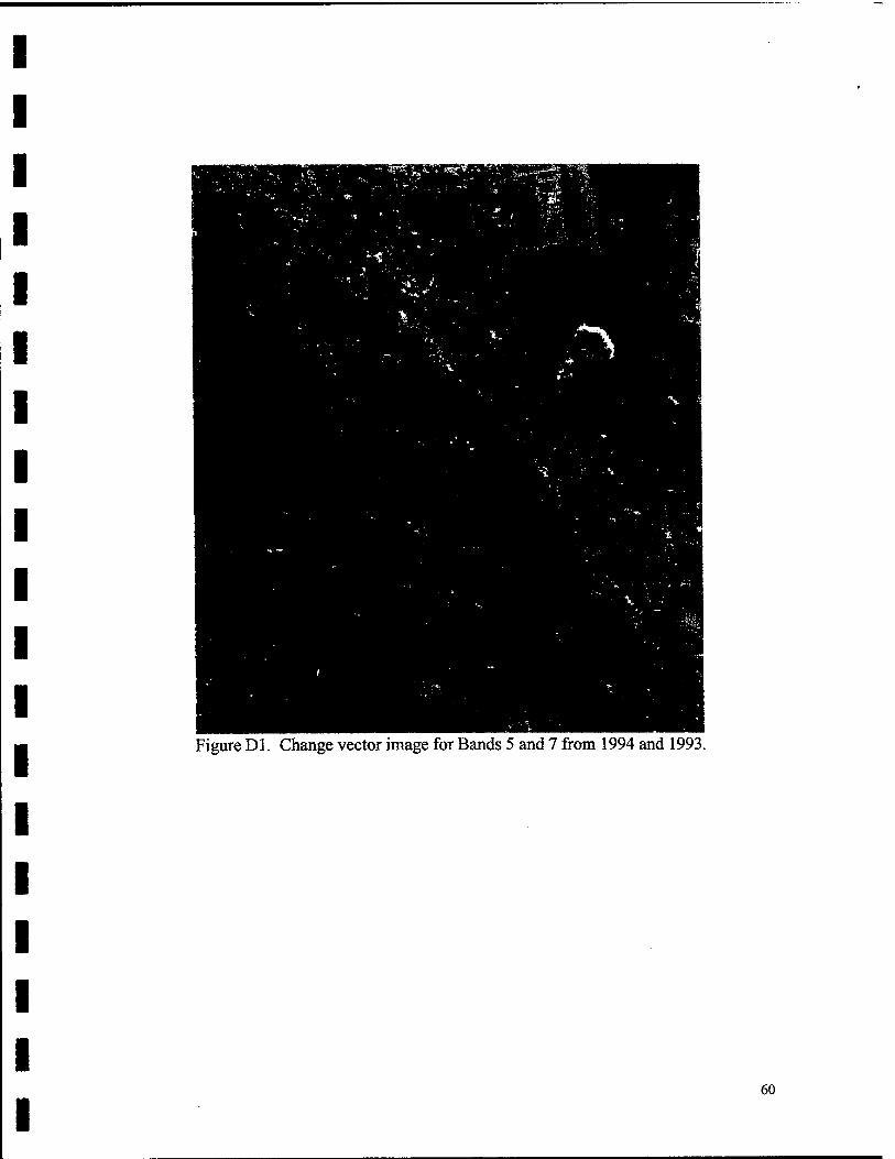
Figure Dl. Change vector image for Bands 5 and 7 from 1994 and 1993
60
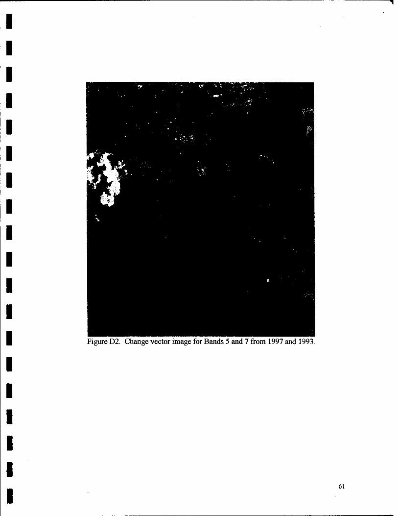
Figure D2. Change vector image for Bands 5 and 7 from 1997 and 1993.
61
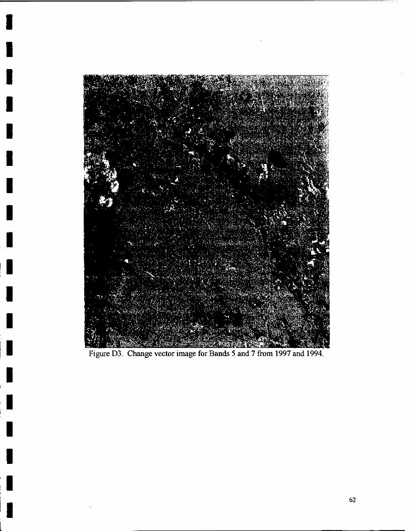
Figure D3. Change vector image for Bands 5 and 7 from 1997 and 1994.
62
REFERENCES
1. Benmouffok, Djilali. "Information for Decision Making." IDRC Reports (Ottowa,
Canada). January 1993, pp. 4-15.
2. Sparks, Richard E. and Ruth. "America Under Water—After Floods: Restoring
Ecosystems." USA Today. July 1994, pp. 40-42.
3. McKibben, Bill. "What Good is a Forest?" Audubon. May/June 1996, pp. 54+.
4. Hartman, Todd. "Creek Creating Havoc: Groups Pouring Resources into Combating
Erosion." Colorado Springs Gazette Telegraph. 30 June 1996, p. Bl.
5. von Guerard, Paul. Suspended Sediment and Sediment-source Areas in the Fountain
Creek Drainage Basin Upstream from Widefield, Southeastern Colorado. U.S.
Geological Survey, Denver, 1989.
6. Rebuffoni, Dean. "Retiring Land Could Help Control Future Damage." Star
Tribune (Minneapolis, Minnesota). May 6,1997, p. Al2.
7. Blankenship, Karl. "Streamside Forests: Keys to the Living Landscape." American
Forests. Spring 1996, pp. 13+.
8. http://www.spaceimage.com/home/overview/profile/si_profile.html
"The Next Generation System."
9. Jessup, Shelby P. and Ernestine Cary. "Geographic Information Systems: What They
Are and How They Work." Focus. Summer 1989. pp. 10-12.
10. Photogrammetric Engineering and Remote Sensing. Vol. 63, January 1997,
pp. 87-93.
11. Constance, Paul. "Remote Sensing Use Expands to City Planning." Aviation Week
and Space Technology. 19 September 1994, pp. 54-55.
63
12. Kiefer, Ralph W. and Thomas M. Lillesand. Remote Sensing and Image
Interpretation. John Wiley and Sons, Inc., New York, 1994.
13. Blaszczynski, Jacek S. "Landform Characterization with GIS." Photogrammetric
Engineering and Remote Sensing. Vol. 63, February 1997, pp. 183-191.
14. Bhatt, Gita. "Remote Sensing in Economic Development." Finance and
Development. June 1992, pp. 45-47.
15. http://www.csc.noaa.gov/ccap/text/protocol.html
"NOAA Coastal Change Analysis Program (C-CAP)."
16. http://ltpwww.gsfc.nasa.gov/ISSSR-95/digitalc.htm
17. http://eol5a.erim.org/EIT/chgdet/chgdet.html
"Change Detection at ERTM."
18. http://157.182.168.10/geog455/spring97/06methods.htm
64
ABSTRACT
Remote sensing methodology and GIS technology provide the resources needed
to gain an improved understanding of the Earth as a system. Worldwide population
growth and development amplify the naturally occurring changes on the Earth's surface
and give birth to new types of changes. With the help of remote sensing technology, the
energy radiated by surface features or reflected off the Earth's surface by the sun can be
used to map the land and trace the changes that take place over time. GIS technology can
then be used to integrate large amounts of image data and other related details about an
area to analyze the changes and their origin.
This paper discusses the methodology and analytical techniques used to process
digital images with a focus on change detection processes. It also emphasizes many of the
atmospheric affects that must be considered before analysis can begin or inferences can be
made. In addition, a change detection analysis of a region of Fountain Creek in Colorado
Springs is performed using LANDSAT TM images gathered in 1993,1994, and 1997.
The analysis provides an example of the application of many of the techniques initially
discussed and also highlights the cautions that were taken to avoid false conclusions. The
investigation includes the generation of change detection images produced using image
algebra and change vector analysis.
ABSTRACT
Remote sensing methodology and GIS technology provide the resources needed
to gain an improved understanding of the Earth as a system. Worldwide population
growth and development amplify the naturally occurring changes on the Earth's surface
and give birth to new types of changes. With the help of remote sensing technology, the
energy radiated by surface features or reflected off the Earth's surface by the sun can be
used to map the land and trace the changes that take place over time. GIS technology can
then be used to integrate large amounts of image data and other related details about an
area to analyze the changes and their origin.
This paper discusses the methodology and analytical techniques used to process
digital images with a focus on change detection processes. It also emphasizes many of the
atmospheric affects that must be considered before analysis can begin or inferences can be
made. In addition, a change detection analysis of a region of Fountain Creek in Colorado
Springs is performed using LANDS AT TM images gathered in 1993,1994, and 1997.
The analysis provides an example of the application of many of the techniques initially
discussed and also highlights the cautions that were taken to avoid false conclusions. The
investigation includes the generation of change detection images produced using image
algebra and change vector analysis.
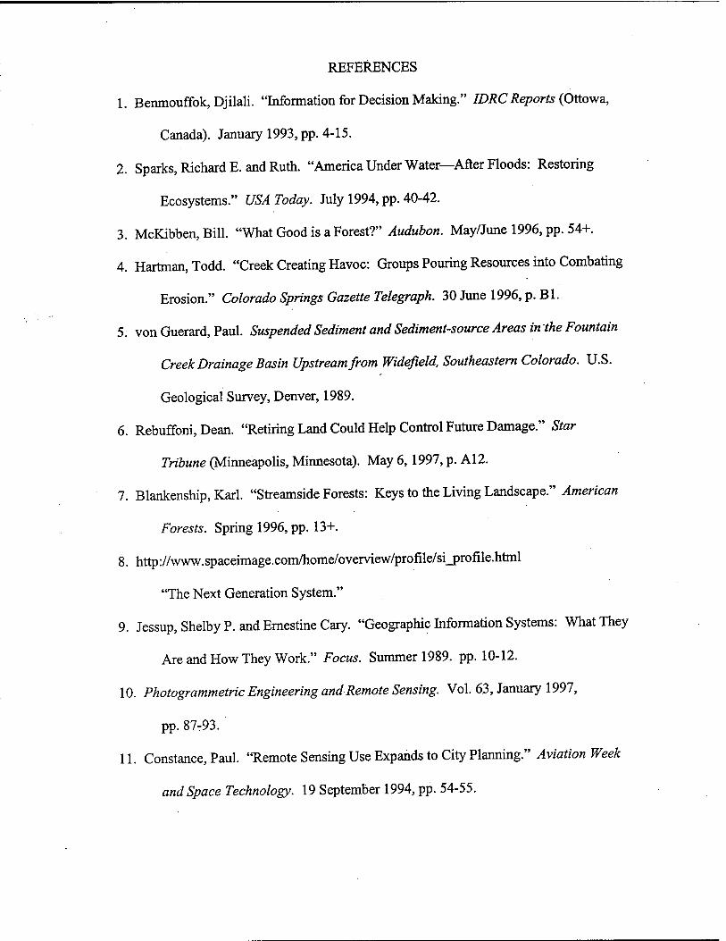
REFERENCES
1. Benmouffok, Djilali. "Information for Decision Making." IDRC Reports (Ottawa,
Canada). January 1993, pp. 4-15.
2. Sparks, Richard E. and Ruth. "America Under Water—After Floods: Restoring
Ecosystems." USA Today. July 1994, pp. 40-42.
3. McKibben, Bill. "What Good is a Forest?" Audubon. May/June 1996, pp. 54+.
4. Hartman, Todd. "Creek Creating Havoc: Groups Pouring Resources into Combating
Erosion." Colorado Springs Gazette Telegraph. 30 June 1996, p. Bl.
5. von Guerard, Paul. Suspended Sediment and Sediment-source Areas in the Fountain
Creek Drainage Basin Upstream from Widefield, Southeastern Colorado. U.S.
Geological Survey, Denver, 1989.
6. Rebuffoni, Dean. "Retiring Land Could Help Control Future Damage." Star
Tribune (Minneapolis, Minnesota). May 6,1997, p. A12.
7. Blankenship, Karl. "Streamside Forests: Keys to the Living Landscape." American
Forests. Spring 1996, pp. 13+.
8. http://www.spaceimage.com/home/overview/profile/sijprofile.html
"The Next Generation System."
9. Jessup, Shelby P. and Ernestine Cary. "Geographic Information Systems: What They
Are and How They Work." Focus. Summer 1989. pp. 10-12.
10. Photogrammetric Engineering and Remote Sensing. Vol. 63, January 1997,
pp.87-93.
11. Constance, Paul. "Remote Sensing Use Expands to City Planning." Aviation Week
and Space Technology. 19 September 1994, pp. 54-55.

12. Kiefer, Ralph W. and Thomas M. Lillesand. Remote Sensing and Image
Interpretation. John Wiley and Sons, Inc., New York, 1994.
13. Blaszczynski, Jacek S. "Landform Characterization with GIS." Photogrammetric
Engineering and Remote Sensing. Vol. 63, February 1997, pp. 183-191.
14. Bhatt, Gita. "Remote Sensing in Economic Development." Finance and
Development. June 1992, pp. 45-47.
15. http://www.csc.noaa.gov/ccap/text/protocol.html
"NOAA Coastal Change Analysis Program (C-CAP)."
16. http://ltpwww.gsfc.nasa.gov/ISSSR-95/digitalc.htm
17. http://eol5a.erim.org/EIT/chgdet/chgdet.html
"Change Detection at ERTM."
18. http://157.182.168.10/geog455/spring97/06methods.htm
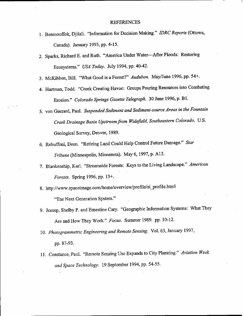
REFERENCES
1. Benmouffok, Djilali. "Information for Decision Making." IDRC Reports (Ottawa,
Canada). January 1993, pp. 4-15.
2. Sparks, Richard E. and Ruth. "America Under Water—After Floods: Restoring
Ecosystems." USA Today. July 1994, pp. 40-42.
3. McKibben, Bill. "What Good is a Forest?" Audubon. May/June 1996, pp. 54+.
4. Hartman, Todd. "Creek Creating Havoc: Groups Pouring Resources into Combating
Erosion." Colorado Springs Gazette Telegraph. 30 June 1996, p. Bl.
5. von Guerard, Paul. Suspended Sediment and Sediment-source Areas in the Fountain
Creek Drainage Basin Upstream from Widefield, Southeastern Colorado. U.S.
Geological Survey, Denver, 1989.
6. Rebuffoni, Dean. "Retiring Land Could Help Control Future Damage." Star
Tribune (Minneapolis, Minnesota). May 6,1997, p. A12.
7. Blankenship, Karl. "Streamside Forests: Keys to the Living Landscape." American
Forests. Spring 1996, pp. 13+.
8. http://www.spaceimage.com/home/overview/profile/si_profile.html
"The Next Generation System."
9. Jessup, Shelby P. and Ernestine Cary. "Geographic Information Systems: What They
Are and How They Work." Focus. Summer 1989. pp. 10-12.
10. Photogrammetric Engineering and Remote Sensing. Vol. 63, January 1997,
pp. 87-93.
11. Constance, Paul. "Remote Sensing Use Expands to City Planning." Aviation Week
and Space Technology. 19 September 1994, pp. 54-55.
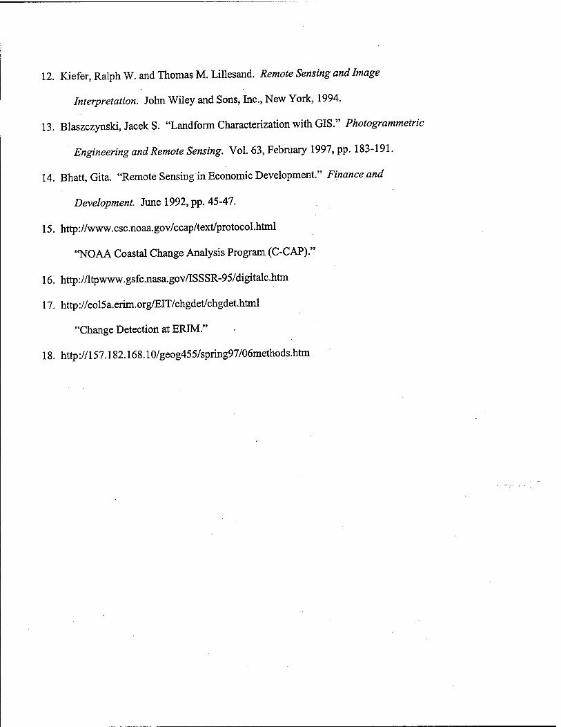
12. Kiefer, Ralph W. and Thomas M. Lillesand. Remote Sensing and Image
Interpretation. John Wiley and Sons, Inc., New York, 1994.
13. Blaszczynski, Jacek S. "Landform Characterization with GIS." Photogrammetric
Engineering and Remote Sensing. Vol. 63, February 1997, pp. 183-191.
14. Bhatt, Gita. "Remote Sensing in Economic Development." Finance and
Development. June 1992, pp. 45-47.
15. http://www.csc.noaa.gov/ccap/text/protocol.html
"NOAA Coastal Change Analysis Program (C-CAP)."
16. http://ltpwww.gsfc.nasa.gov/ISSSR-95/digitalc.htm
17. http://eol5a.erim.org/EIT/chgdet/chgdet.html
"Change Detection at ERIM."
18. http://157.182.168.10/geog455/spring97/06methods.htm


![Satellite Imagery Product Specificationslps16.esa.int/posterfiles/paper1213/[RD16]_RE_Product... · 2016-04-22 · Satellite Imagery Product Specifications 6 2 RAPIDEYE SATELLITE](https://img.pdfslide.net/doc/110x75/5eba16697328255ddd5746a8/satellite-imagery-product-rd16reproduct-2016-04-22-satellite-imagery-product.jpg)