Embed Size (px)
Citation preview
11 - 1Fundamentals of Kalman Filtering:A Practical Approach
Satellite Navigation
11 - 2Fundamentals of Kalman Filtering:A Practical Approach
Satellite NavigationOverview
• Solving for receiver location based on perfect rangemeasurements from two satellites• Solving for receiver location based on noisy rangemeasurements from two satellites (no filtering)• Improvements with linear filtering of range• Using extended Kalman filter• Using extended Kalman filter with measurements from only onesatellite• Moving receiver
- Constant velocity- Variable velocity
11 - 3Fundamentals of Kalman Filtering:A Practical Approach
Solving for Receiver Location Based on PerfectRange Measurements From Two Satellites
11 - 4Fundamentals of Kalman Filtering:A Practical Approach
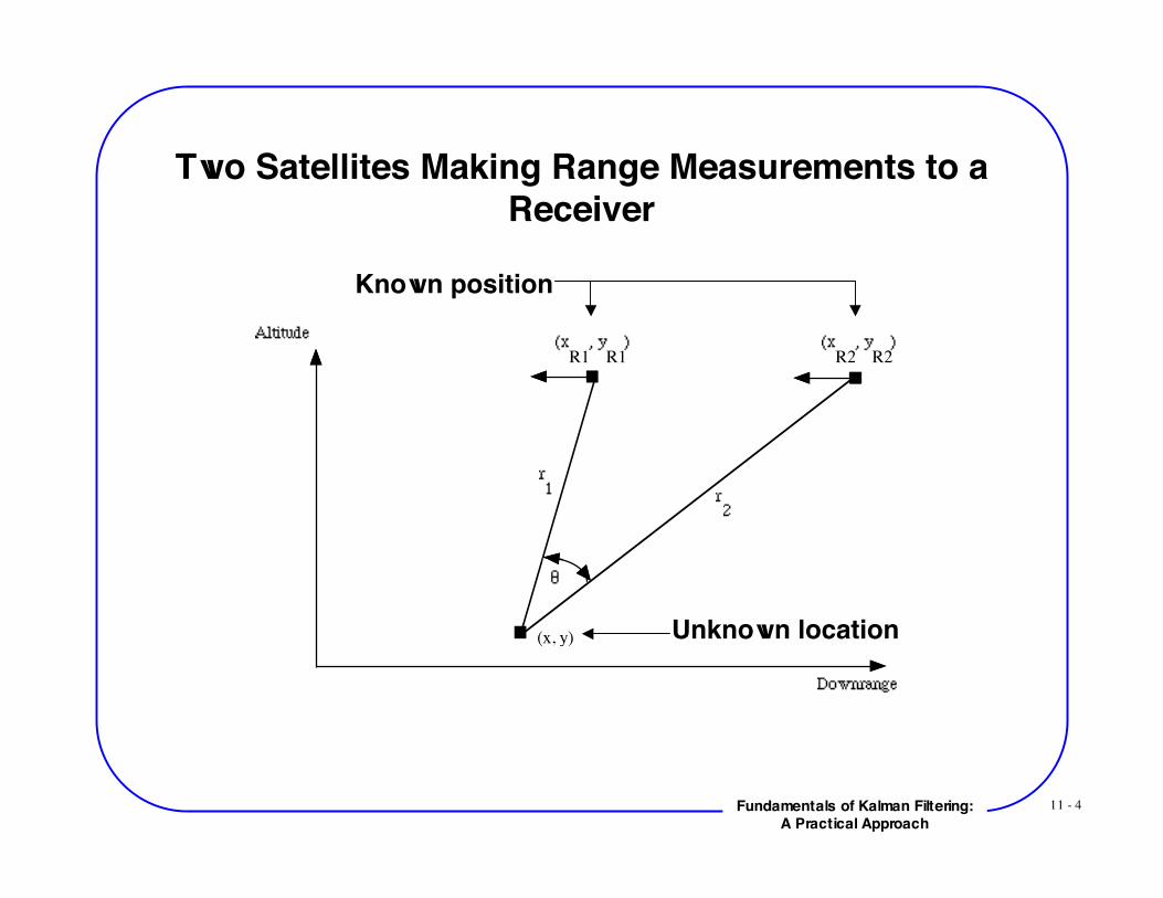
Two Satellites Making Range Measurements to aReceiver
R1 R1 R2R2
(x, y)
Known position
Unknown location
11 - 5Fundamentals of Kalman Filtering:A Practical Approach
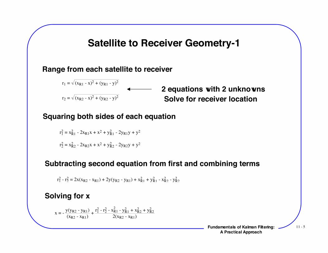
Satellite to Receiver Geometry-1
r1 = (xR1 - x)2 + (yR1 - y)2
Range from each satellite to receiver
r2 = (xR2 - x)2 + (yR2 - y)2
2 equations with 2 unknowns
Squaring both sides of each equation
r12 = xR1
2 - 2xR1x + x2 + yR12 - 2yR1y + y2
Solve for receiver location
r22 = xR2
2 - 2xR2x + x2 + yR22 - 2yR2y + y2
Subtracting second equation from first and combining terms
r12 - r2
2 = 2x(xR2 - xR1) + 2y(yR2 - yR1) + xR12 + yR1
2 - xR22 - yR2
2
Solving for x
x = - y(yR2 - yR1)
(xR2 - xR1) +
r12 - r2
2 - xR12
- yR12 + xR2
2 + yR22
2(xR2 - xR1)
11 - 6Fundamentals of Kalman Filtering:A Practical Approach
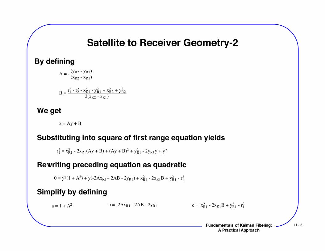
Satellite to Receiver Geometry-2By defining
A = - (yR2 - yR1)
(xR2 - xR1)
B = r12 - r2
2 - xR12
- yR12 + xR2
2 + yR22
2(xR2 - xR1)
We getx = Ay + B
Substituting into square of first range equation yieldsr12 = xR1
2 - 2xR1(Ay + B) + (Ay + B)2 + yR12 - 2yR1y + y2
Rewriting preceding equation as quadratic0 = y2(1 + A2) + y(-2AxR1+ 2AB - 2yR1) + xR1
2 - 2xR1B + yR12 - r1
2
Simplify by defininga = 1 + A2 b = -2AxR1+ 2AB - 2yR1 c = xR1
2 - 2xR1B + yR12 - r1
2
11 - 7Fundamentals of Kalman Filtering:A Practical Approach
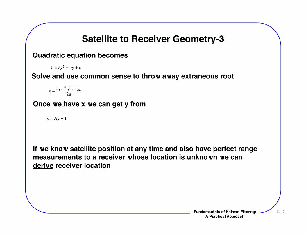
Satellite to Receiver Geometry-3Quadratic equation becomes
0 = ay2 + by + c
Solve and use common sense to throw away extraneous root
y = -b - b2 - 4ac2a
Once we have x we can get y from
x = Ay + B
If we know satellite position at any time and also have perfect rangemeasurements to a receiver whose location is unknown we canderive receiver location
11 - 8Fundamentals of Kalman Filtering:A Practical Approach
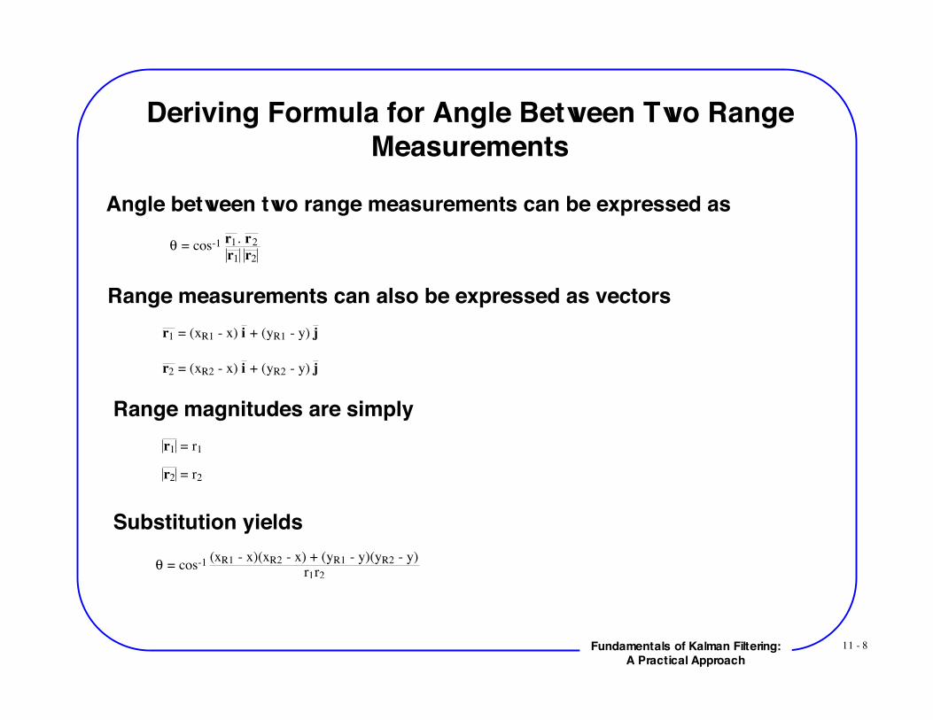
Deriving Formula for Angle Between Two RangeMeasurements
Angle between two range measurements can be expressed as! = cos-1
r1. r2
r1 r2
Range measurements can also be expressed as vectorsr1 = (xR1 - x) i + (yR1 - y) j
r2 = (xR2 - x) i + (yR2 - y) j
Range magnitudes are simplyr1 = r1
r2 = r2
Substitution yields
! = cos-1 (xR1 - x)(xR2 - x) + (yR1 - y)(yR2 - y)r1r2
11 - 9Fundamentals of Kalman Filtering:A Practical Approach
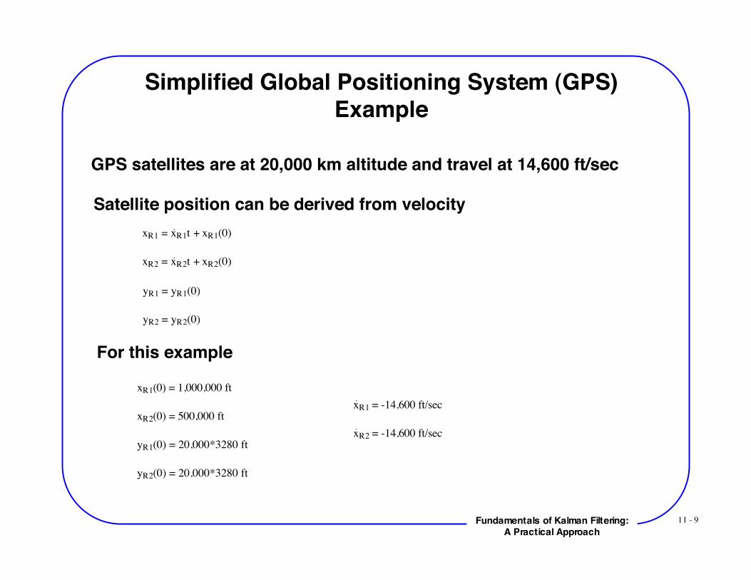
Simplified Global Positioning System (GPS)Example
GPS satellites are at 20,000 km altitude and travel at 14,600 ft/sec
Satellite position can be derived from velocity
yR1 = yR1(0)
yR2 = yR2(0)
For this example
xR1(0) = 1,000,000 ft
xR2(0) = 500,000 ft
yR1(0) = 20,000*3280 ft
yR2(0) = 20,000*3280 ft
xR1 = -14,600 ft/sec
xR2 = -14,600 ft/sec
xR1 = xR1t + xR1(0)
xR2 = xR2t + xR2(0)
11 - 10Fundamentals of Kalman Filtering:A Practical Approach
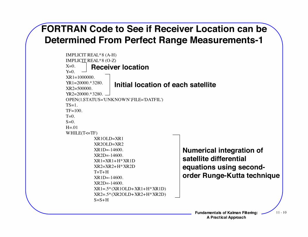
FORTRAN Code to See if Receiver Location can beDetermined From Perfect Range Measurements-1
IMPLICIT REAL*8 (A-H)IMPLICIT REAL*8 (O-Z)X=0.Y=0.XR1=1000000.YR1=20000.*3280.XR2=500000.YR2=20000.*3280.OPEN(1,STATUS='UNKNOWN',FILE='DATFIL')TS=1.TF=100.T=0.S=0.H=.01WHILE(T<=TF)
XR1OLD=XR1XR2OLD=XR2
XR1D=-14600.XR2D=-14600.
XR1=XR1+H*XR1DXR2=XR2+H*XR2D
T=T+HXR1D=-14600.XR2D=-14600.
XR1=.5*(XR1OLD+XR1+H*XR1D)XR2=.5*(XR2OLD+XR2+H*XR2D)
S=S+H
Receiver location
Initial location of each satellite
Numerical integration ofsatellite differentialequations using second-order Runge-Kutta technique
11 - 11Fundamentals of Kalman Filtering:A Practical Approach
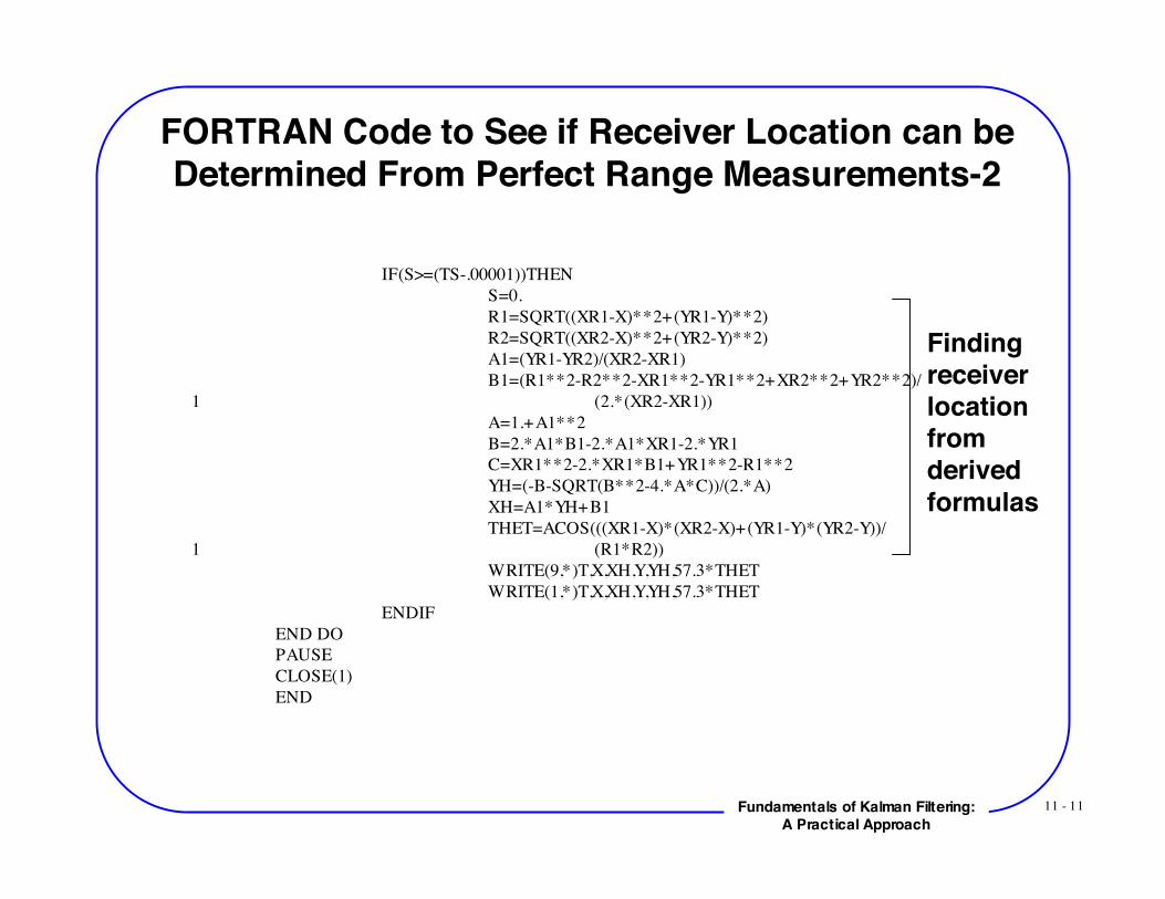
FORTRAN Code to See if Receiver Location can beDetermined From Perfect Range Measurements-2
IF(S>=(TS-.00001))THENS=0.R1=SQRT((XR1-X)**2+(YR1-Y)**2)R2=SQRT((XR2-X)**2+(YR2-Y)**2)A1=(YR1-YR2)/(XR2-XR1)B1=(R1**2-R2**2-XR1**2-YR1**2+XR2**2+YR2**2)/
1 (2.*(XR2-XR1))A=1.+A1**2B=2.*A1*B1-2.*A1*XR1-2.*YR1C=XR1**2-2.*XR1*B1+YR1**2-R1**2YH=(-B-SQRT(B**2-4.*A*C))/(2.*A)XH=A1*YH+B1THET=ACOS(((XR1-X)*(XR2-X)+(YR1-Y)*(YR2-Y))/
1 (R1*R2))WRITE(9,*)T,X,XH,Y,YH,57.3*THETWRITE(1,*)T,X,XH,Y,YH,57.3*THET
ENDIFEND DO
PAUSECLOSE(1)END
Findingreceiverlocationfromderivedformulas
11 - 12Fundamentals of Kalman Filtering:A Practical Approach
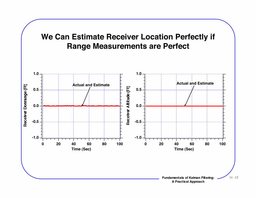
We Can Estimate Receiver Location Perfectly ifRange Measurements are Perfect
-1.0
-0.5
0.0
0.5
1.0
100806040200
Time (Sec)
Actual and Estimate
-1.0
-0.5
0.0
0.5
1.0
100806040200
Time (Sec)
Actual and Estimate
11 - 13Fundamentals of Kalman Filtering:A Practical Approach
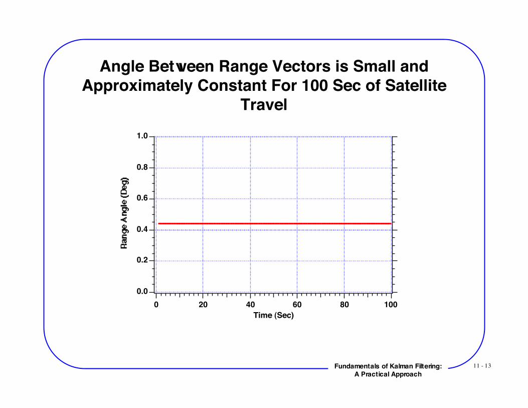
Angle Between Range Vectors is Small andApproximately Constant For 100 Sec of Satellite
Travel1.0
0.8
0.6
0.4
0.2
0.0
100806040200
Time (Sec)

11 - 14Fundamentals of Kalman Filtering:A Practical Approach
Solving for Receiver Location Based on NoisyRange Measurements From Two Satellites (No
Filtering)
11 - 15Fundamentals of Kalman Filtering:A Practical Approach
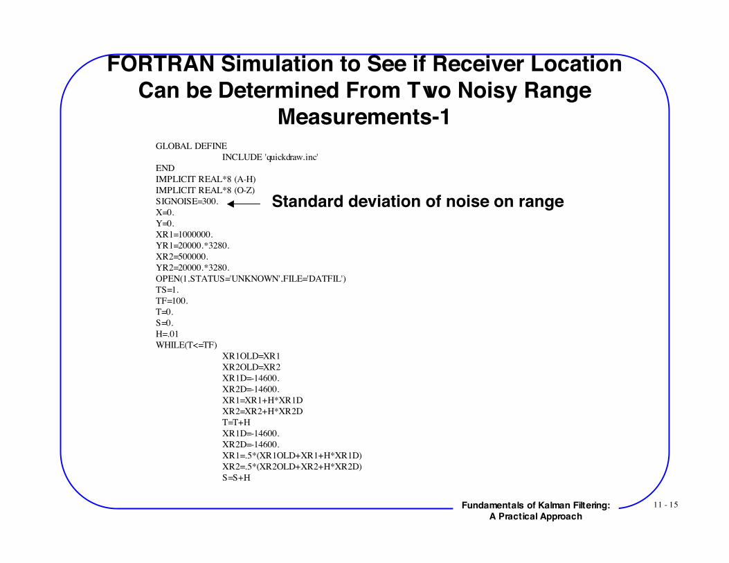
FORTRAN Simulation to See if Receiver LocationCan be Determined From Two Noisy Range
Measurements-1GLOBAL DEFINE
INCLUDE 'quickdraw.inc' END
IMPLICIT REAL*8 (A-H)IMPLICIT REAL*8 (O-Z)SIGNOISE=300.X=0.Y=0.XR1=1000000.YR1=20000.*3280.XR2=500000.YR2=20000.*3280.OPEN(1,STATUS='UNKNOWN',FILE='DATFIL')TS=1.TF=100.T=0.S=0.H=.01WHILE(T<=TF)
XR1OLD=XR1XR2OLD=XR2XR1D=-14600.XR2D=-14600.
XR1=XR1+H*XR1DXR2=XR2+H*XR2D
T=T+HXR1D=-14600.XR2D=-14600.
XR1=.5*(XR1OLD+XR1+H*XR1D)XR2=.5*(XR2OLD+XR2+H*XR2D)
S=S+H
Standard deviation of noise on range

11 - 16Fundamentals of Kalman Filtering:A Practical Approach
FORTRAN Simulation to See if Receiver LocationCan be Determined From Two Noisy Range
Measurements-2
IF(S>=(TS-.00001))THENS=0.CALL GAUSS(R1NOISE,SIGNOISE)CALL GAUSS(R2NOISE,SIGNOISE)R1=SQRT((XR1-X)**2+(YR1-Y)**2)R2=SQRT((XR2-X)**2+(YR2-Y)**2)R1S=R1+R1NOISER2S=R2+R2NOISEA1=(YR1-YR2)/(XR2-XR1)B1=(R1S**2-R2S**2-XR1**2-YR1**2+XR2**2+YR2**2)/
1 (2.*(XR2-XR1))A=1.+A1**2B=2.*A1*B1-2.*A1*XR1-2.*YR1C=XR1**2-2.*XR1*B1+YR1**2-R1S**2YH=(-B-SQRT(B**2-4.*A*C))/(2.*A)XH=A1*YH+B1THET=ACOS(((XR1-X)*(XR2-X)+(YR1-Y)*(YR2-Y))/
1 (R1*R2))WRITE(9,*)T,X,XH,Y,YH,57.3*THET,R1,R2WRITE(1,*)T,X,XH,Y,YH,57.3*THET,R1,R2
ENDIFEND DO
PAUSECLOSE(1)END
Noisy rangemeasurements
11 - 17Fundamentals of Kalman Filtering:A Practical Approach
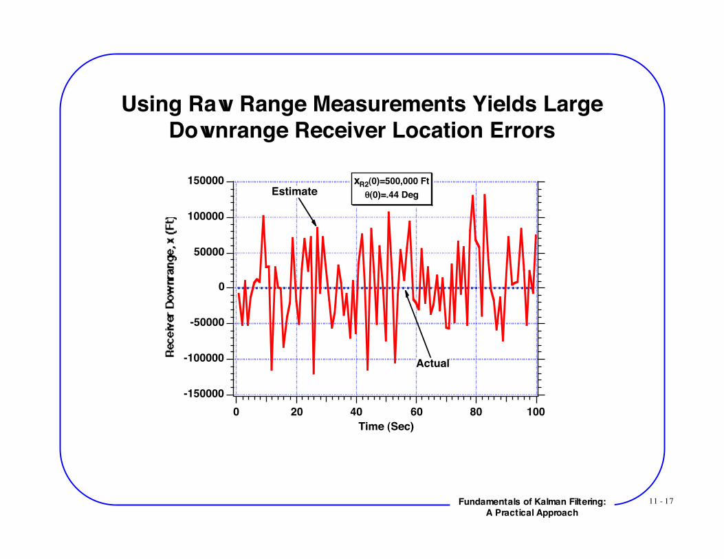
Using Raw Range Measurements Yields LargeDownrange Receiver Location Errors
-150000
-100000
-50000
0
50000
100000
150000
100806040200
Time (Sec)
Actual
EstimatexR2(0)=500,000 Ft
!(0)=.44 Deg
11 - 18Fundamentals of Kalman Filtering:A Practical Approach
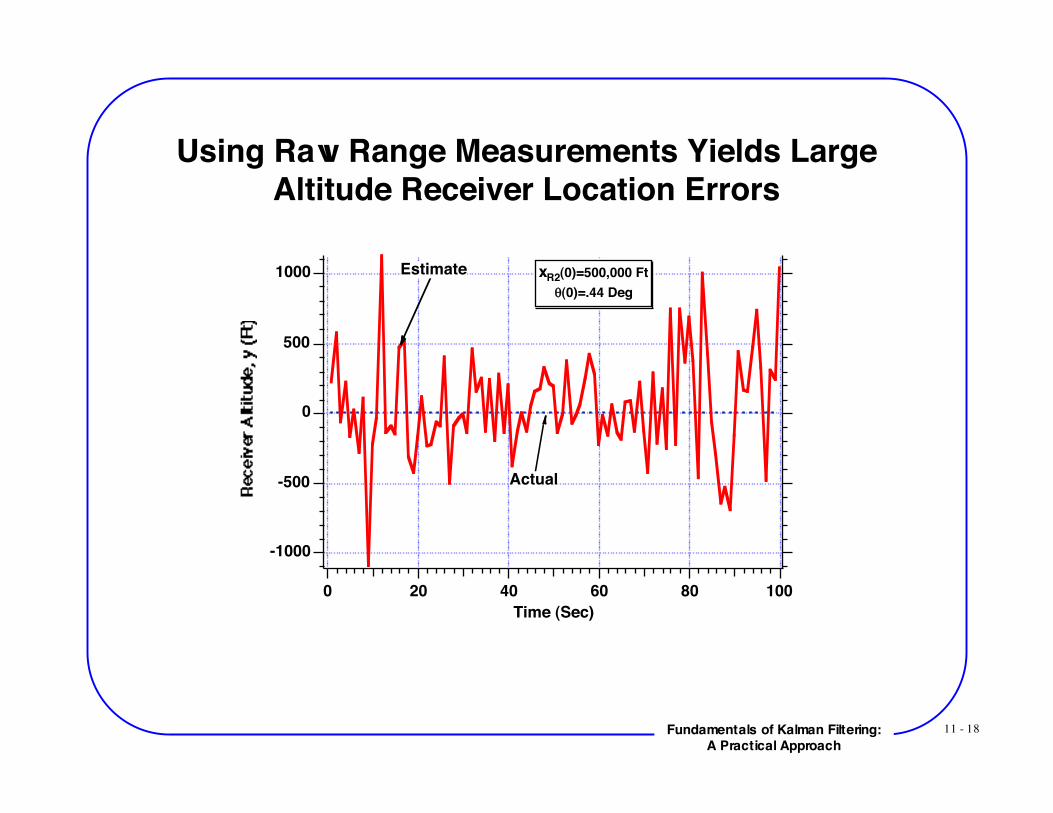
Using Raw Range Measurements Yields LargeAltitude Receiver Location Errors
1000
500
0
-500
-1000
100806040200
Time (Sec)
xR2(0)=500,000 Ft
!(0)=.44 Deg
Actual
Estimate
11 - 19Fundamentals of Kalman Filtering:A Practical Approach
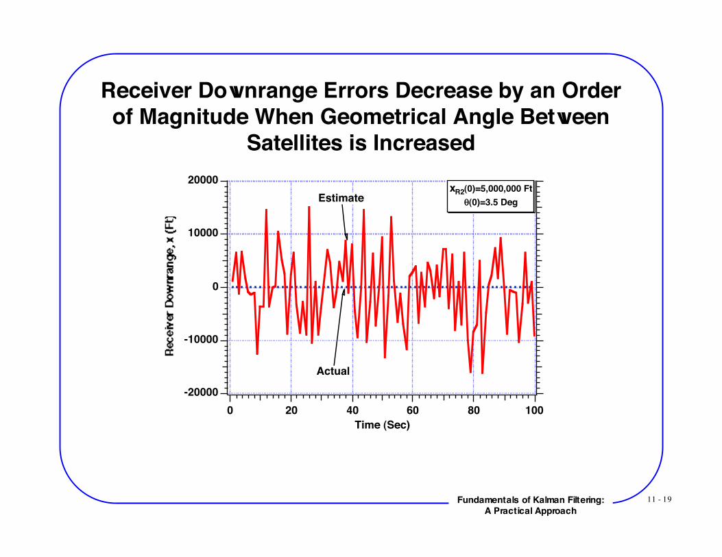
Receiver Downrange Errors Decrease by an Orderof Magnitude When Geometrical Angle Between
Satellites is Increased
-20000
-10000
0
10000
20000
100806040200
Time (Sec)
xR2(0)=5,000,000 Ft
!(0)=3.5 Deg
Actual
Estimate
11 - 20Fundamentals of Kalman Filtering:A Practical Approach
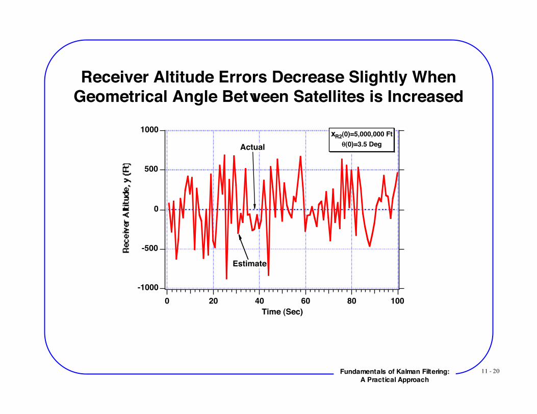
Receiver Altitude Errors Decrease Slightly WhenGeometrical Angle Between Satellites is Increased
-1000
-500
0
500
1000
100806040200
Time (Sec)
xR2(0)=5,000,000 Ft
!(0)=3.5 DegActual
Estimate
11 - 21Fundamentals of Kalman Filtering:A Practical Approach
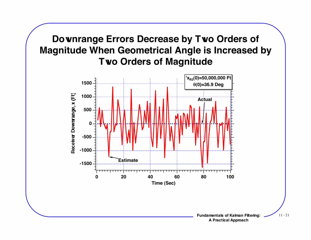
Downrange Errors Decrease by Two Orders ofMagnitude When Geometrical Angle is Increased by
Two Orders of Magnitude
-1500
-1000
-500
0
500
1000
1500
100806040200
Time (Sec)
'xR2(0)=50,000,000 Ft
!(0)=36.9 Deg
Actual
Estimate
11 - 22Fundamentals of Kalman Filtering:A Practical Approach
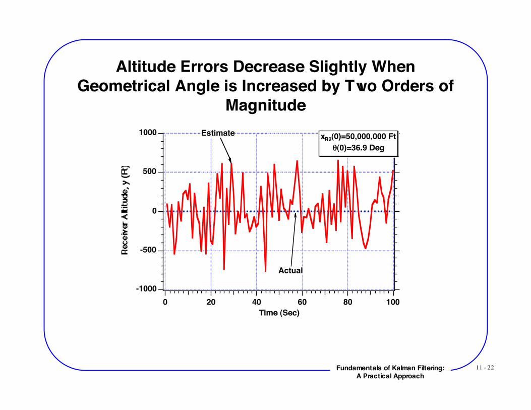
Altitude Errors Decrease Slightly WhenGeometrical Angle is Increased by Two Orders of
Magnitude
-1000
-500
0
500
1000
100806040200
Time (Sec)
xR2(0)=50,000,000 Ft
!(0)=36.9 Deg
Actual
Estimate
11 - 23Fundamentals of Kalman Filtering:A Practical Approach
Summary When Filtering is Not Used
• Downrange errors decrease when range angle increases• Altitude errors have weak dependence on range angle• In best geometry range angle approaches 90 deg
11 - 24Fundamentals of Kalman Filtering:A Practical Approach
Improvements With Linear Filtering of Range
11 - 25Fundamentals of Kalman Filtering:A Practical Approach
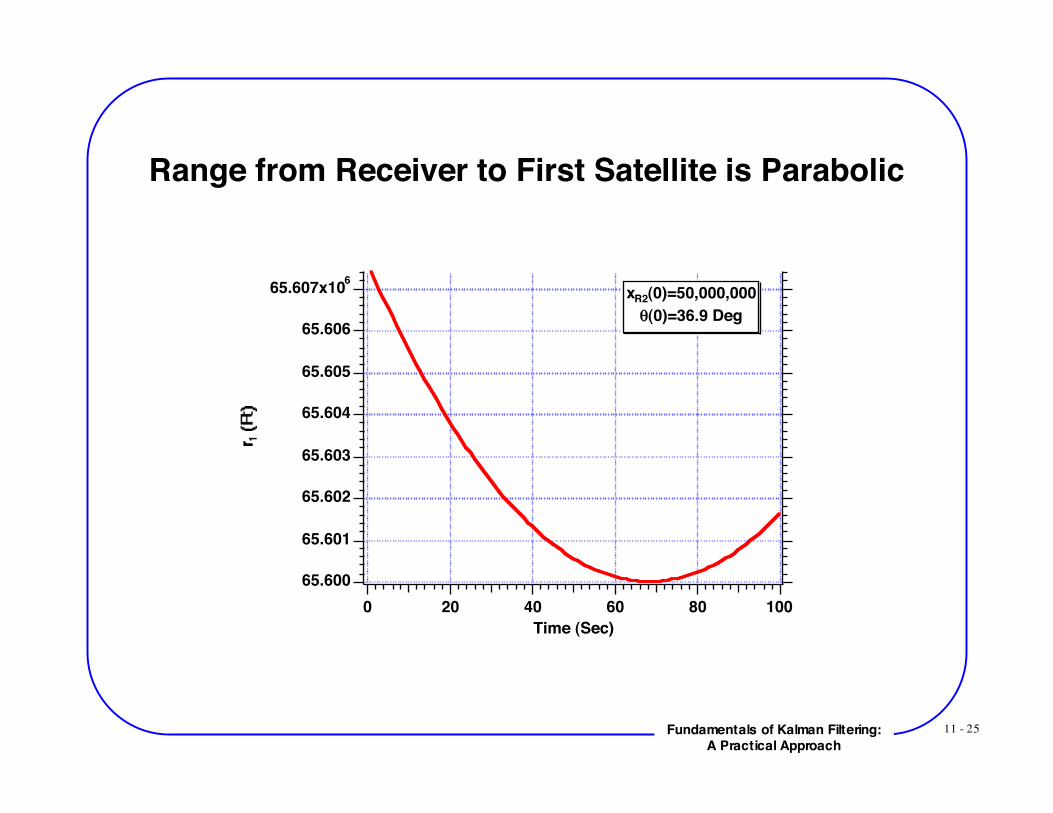
Range from Receiver to First Satellite is Parabolic
65.607x10⁶
65.606
65.605
65.604
65.603
65.602
65.601
65.600100806040200
Time (Sec)
xR2(0)=50,000,000θ(0)=36.9 Deg

11 - 26Fundamentals of Kalman Filtering:A Practical Approach
Range From Receiver to Second Satellite is aStraight Line
We will play it safe and use second-order recursive least squaresfilter on each set of range measurements
82.4x10⁶
82.2
82.0
81.8
100806040200Time (Sec)
xR2(0)=50,000,000θ(0)=36.9 Deg
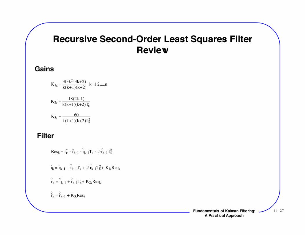
11 - 27Fundamentals of Kalman Filtering:A Practical Approach
Recursive Second-Order Least Squares FilterReview
Gains
K1k =
3(3k2-3k+2)
k(k+1)(k+2) k=1,2,...,n
K2k =
18(2k-1)
k(k+1)(k+2)Ts
K3k = 60
k(k+1)(k+2)Ts2
Filter
Resk = rk* - rk-1 - rk-1Ts - .5rk-1Ts
2
rk = rk-1 + rk-1Ts + .5rk-1Ts2+ K1k
Resk
rk = rk-1 + rk-1Ts+ K2kResk
rk = rk-1 + K3kResk
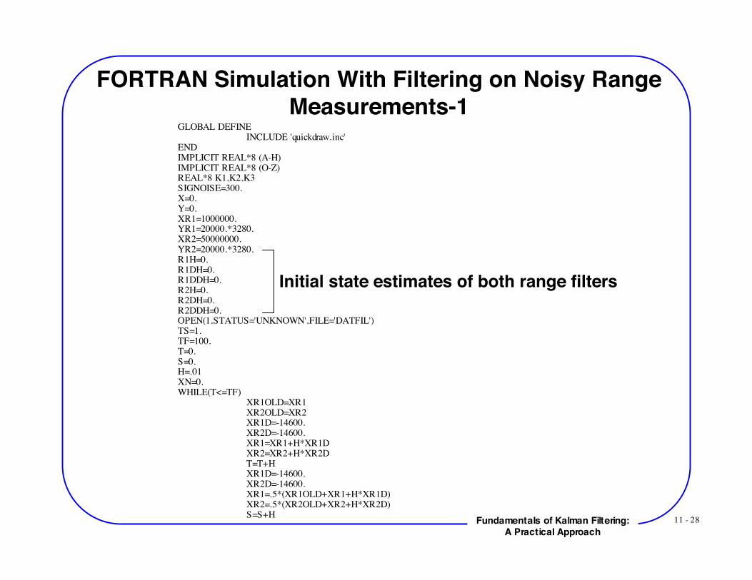
11 - 28Fundamentals of Kalman Filtering:A Practical Approach
FORTRAN Simulation With Filtering on Noisy RangeMeasurements-1
GLOBAL DEFINE INCLUDE 'quickdraw.inc' END
IMPLICIT REAL*8 (A-H)IMPLICIT REAL*8 (O-Z)REAL*8 K1,K2,K3SIGNOISE=300.X=0.Y=0.XR1=1000000.YR1=20000.*3280.XR2=50000000.YR2=20000.*3280.R1H=0.R1DH=0.R1DDH=0.R2H=0.R2DH=0.R2DDH=0.OPEN(1,STATUS='UNKNOWN',FILE='DATFIL')TS=1.TF=100.T=0.S=0.H=.01XN=0.WHILE(T<=TF)
XR1OLD=XR1XR2OLD=XR2XR1D=-14600.XR2D=-14600.
XR1=XR1+H*XR1DXR2=XR2+H*XR2D
T=T+HXR1D=-14600.XR2D=-14600.
XR1=.5*(XR1OLD+XR1+H*XR1D)XR2=.5*(XR2OLD+XR2+H*XR2D)
S=S+H
Initial state estimates of both range filters
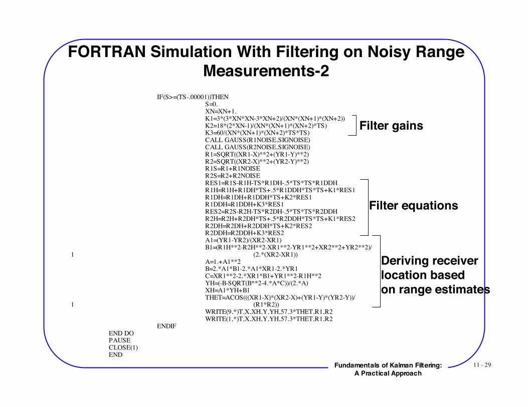
11 - 29Fundamentals of Kalman Filtering:A Practical Approach
FORTRAN Simulation With Filtering on Noisy RangeMeasurements-2
IF(S>=(TS-.00001))THENS=0.XN=XN+1.K1=3*(3*XN*XN-3*XN+2)/(XN*(XN+1)*(XN+2))K2=18*(2*XN-1)/(XN*(XN+1)*(XN+2)*TS)K3=60/(XN*(XN+1)*(XN+2)*TS*TS)CALL GAUSS(R1NOISE,SIGNOISE)CALL GAUSS(R2NOISE,SIGNOISE)R1=SQRT((XR1-X)**2+(YR1-Y)**2)R2=SQRT((XR2-X)**2+(YR2-Y)**2)R1S=R1+R1NOISER2S=R2+R2NOISERES1=R1S-R1H-TS*R1DH-.5*TS*TS*R1DDHR1H=R1H+R1DH*TS+.5*R1DDH*TS*TS+K1*RES1R1DH=R1DH+R1DDH*TS+K2*RES1R1DDH=R1DDH+K3*RES1RES2=R2S-R2H-TS*R2DH-.5*TS*TS*R2DDHR2H=R2H+R2DH*TS+.5*R2DDH*TS*TS+K1*RES2R2DH=R2DH+R2DDH*TS+K2*RES2R2DDH=R2DDH+K3*RES2A1=(YR1-YR2)/(XR2-XR1)B1=(R1H**2-R2H**2-XR1**2-YR1**2+XR2**2+YR2**2)/
1 (2.*(XR2-XR1))A=1.+A1**2B=2.*A1*B1-2.*A1*XR1-2.*YR1C=XR1**2-2.*XR1*B1+YR1**2-R1H**2YH=(-B-SQRT(B**2-4.*A*C))/(2.*A)XH=A1*YH+B1THET=ACOS(((XR1-X)*(XR2-X)+(YR1-Y)*(YR2-Y))/
1 (R1*R2))WRITE(9,*)T,X,XH,Y,YH,57.3*THET,R1,R2WRITE(1,*)T,X,XH,Y,YH,57.3*THET,R1,R2
ENDIFEND DO
PAUSECLOSE(1)END
Filter gains
Filter equations
Deriving receiverlocation basedon range estimates

11 - 30Fundamentals of Kalman Filtering:A Practical Approach
Filtering Range Reduces Receiver DownrangeLocation Errors
-800
-600
-400
-200
0
200
400
600
100806040200
Time (Sec)
xR2(0)=50,000,000
!(0)=36.9 Deg
Actual
Estimate
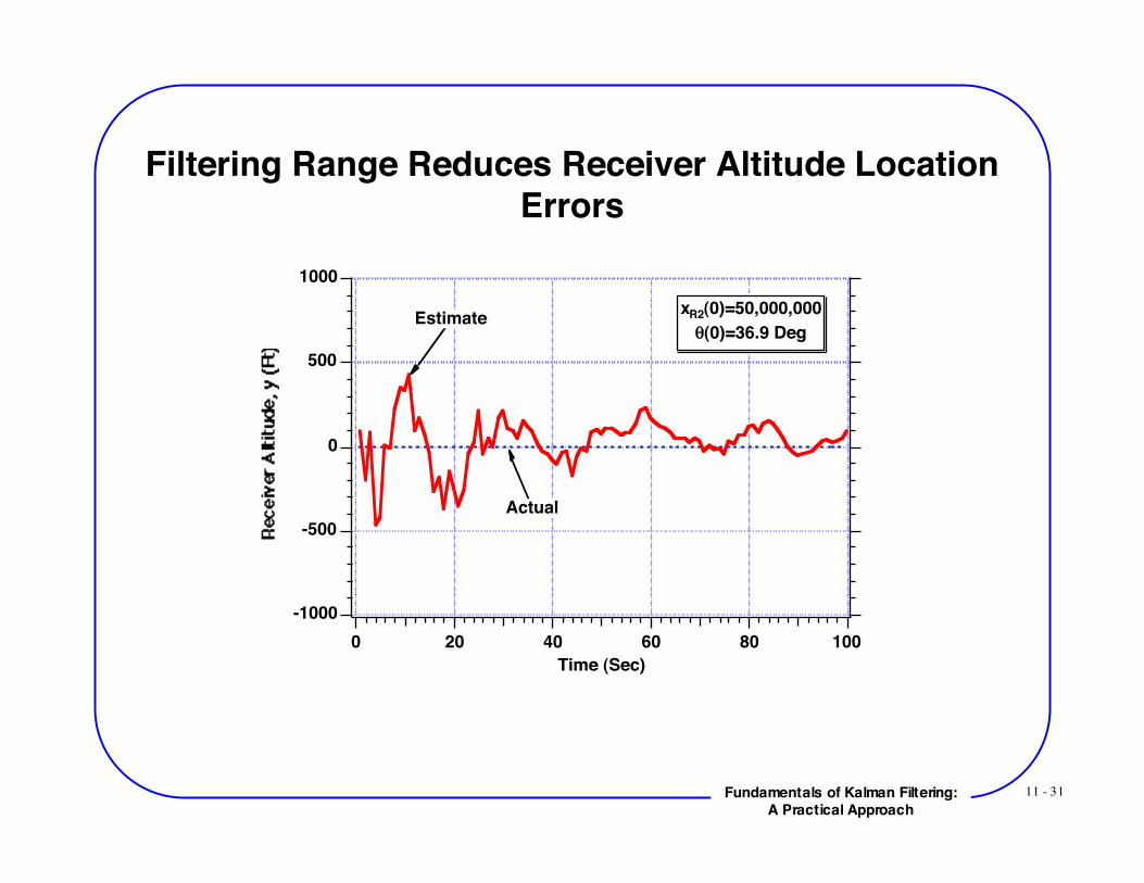
11 - 31Fundamentals of Kalman Filtering:A Practical Approach
Filtering Range Reduces Receiver Altitude LocationErrors
-1000
-500
0
500
1000
100806040200
Time (Sec)
xR2(0)=50,000,000
!(0)=36.9 Deg
Actual
Estimate

11 - 32Fundamentals of Kalman Filtering:A Practical Approach
Using Extended Kalman Filtering

11 - 33Fundamentals of Kalman Filtering:A Practical Approach
Setting Up Problem-1Receiver is stationary
x = 0
y = 0
Or in state space form without process noisex
y = 0 0
0 0
x
y
Therefore systems dynamics matrix is zeroF =
0 0
0 0
Fundamental matrix is identity matrix
!k = 1 0
0 1
Ranges from each satellite to receiverr1 = (xR1 - x)2 + (yR1 - y)2
r2 = (xR2 - x)2 + (yR2 - y)2
11 - 34Fundamentals of Kalman Filtering:A Practical Approach
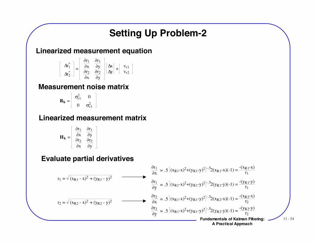
Setting Up Problem-2Linearized measurement equation
!r1*
!r2*
=
"r1
"x
"r1
"y"r2
"x
"r2
"y
!x
!y +
vr1
vr2
Measurement noise matrixRk =
!r1
20
0 !r2
2
Linearized measurement matrix
Hk =
!r1
!x
!r1
!y!r2
!x
!r2
!y
Evaluate partial derivatives
r1 = (xR1 - x)2 + (yR1 - y)2
!r1
!x = .5 (xR1-x)2+(yR1-y)2 -.5
2(xR1-x)(-1) = -(xR1-x)
r1
!r1
!y = .5 (xR1-x)2+(yR1-y)2 -.5
2(yR1-y)(-1) = -(yR1-y)
r1
r2 = (xR2 - x)2 + (yR2 - y)2
!r2
!x = .5 (xR1-x)2+(yR1-y)2 -.5
2(xR2-x)(-1) = -(xR2-x)
r2
!r2
!y = .5 (xR1-x)2+(yR1-y)2 -.5
2(yR2-y)(-1) = -(yR2-y)
r2
11 - 35Fundamentals of Kalman Filtering:A Practical Approach
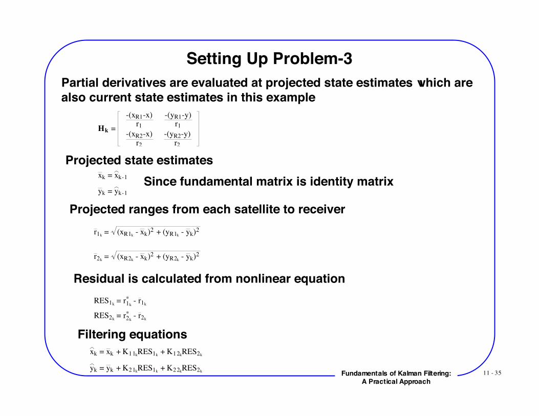
Setting Up Problem-3Partial derivatives are evaluated at projected state estimates which arealso current state estimates in this example
Hk =
-(xR1-x)r1
-(yR1-y)
r1
-(xR2-x)r2
-(yR2-y)r2
Projected state estimatesxk = xk-1
yk = yk-1
Since fundamental matrix is identity matrix
Projected ranges from each satellite to receiverr1k
= (xR1k - xk)2 + (yR1k
- yk)2
r2k = (xR2k
- xk)2 + (yR2k - yk)2
Residual is calculated from nonlinear equationRES1k
= r1k
* - r1k
RES2k = r2k
* - r2k
Filtering equationsxk = xk + K11k
RES1k + K12k
RES2k
yk = yk + K21kRES1k
+ K22kRES2k
11 - 36Fundamentals of Kalman Filtering:A Practical Approach
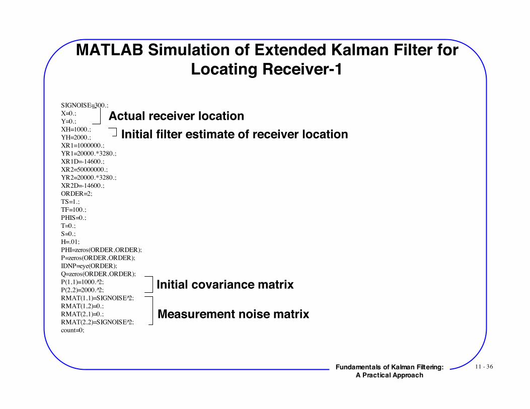
MATLAB Simulation of Extended Kalman Filter forLocating Receiver-1
SIGNOISE=300.;X=0.;Y=0.;XH=1000.;YH=2000.;XR1=1000000.;YR1=20000.*3280.;XR1D=-14600.;XR2=50000000.;YR2=20000.*3280.;XR2D=-14600.;ORDER=2;TS=1.;TF=100.;PHIS=0.;T=0.;S=0.;H=.01;PHI=zeros(ORDER,ORDER);P=zeros(ORDER,ORDER);IDNP=eye(ORDER);Q=zeros(ORDER,ORDER);P(1,1)=1000. 2̂;P(2,2)=2000. 2̂;RMAT(1,1)=SIGNOISE 2̂;RMAT(1,2)=0.;RMAT(2,1)=0.;RMAT(2,2)=SIGNOISE 2̂;count=0;
Initial covariance matrix
Measurement noise matrix
Actual receiver locationInitial filter estimate of receiver location
11 - 37Fundamentals of Kalman Filtering:A Practical Approach
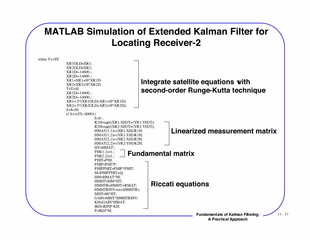
MATLAB Simulation of Extended Kalman Filter forLocating Receiver-2
while T<=TFXR1OLD=XR1;XR2OLD=XR2;
XR1D=-14600.;XR2D=-14600.;
XR1=XR1+H*XR1D;XR2=XR2+H*XR2D;
T=T+H;XR1D=-14600.;XR2D=-14600.;
XR1=.5*(XR1OLD+XR1+H*XR1D);XR2=.5*(XR2OLD+XR2+H*XR2D);
S=S+H;if S>=(TS-.00001)
S=0.;R1H=sqrt((XR1-XH) 2̂+(YR1-YH) 2̂);R2H=sqrt((XR2-XH) 2̂+(YR2-YH) 2̂);HMAT(1,1)=-(XR1-XH)/R1H;HMAT(1,2)=-(YR1-YH)/R1H;HMAT(2,1)=-(XR2-XH)/R2H;HMAT(2,2)=-(YR2-YH)/R2H;HT=HMAT';PHI(1,1)=1.;PHI(2,2)=1.;PHIT=PHI;
PHIP=PHI*P; PHIPPHIT=PHIP*PHIT; M=PHIPPHIT+Q; HM=HMAT*M; HMHT=HM*HT; HMHTR=HMHT+RMAT;
HMHTRINV=inv(HMHTR);MHT=M*HT;
GAIN=MHT*HMHTRINV;KH=GAIN*HMAT;
IKH=IDNP-KH; P=IKH*M;
Integrate satellite equations withsecond-order Runge-Kutta technique
Linearized measurement matrix
Fundamental matrix
Riccati equations
11 - 38Fundamentals of Kalman Filtering:A Practical Approach
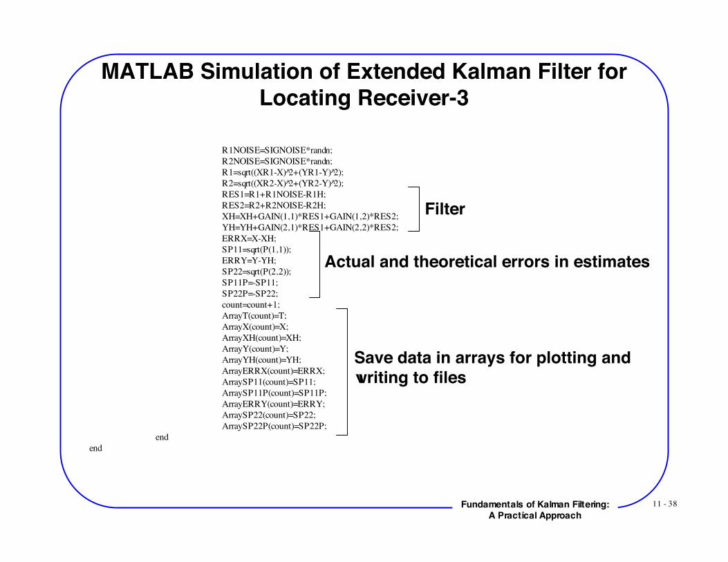
MATLAB Simulation of Extended Kalman Filter forLocating Receiver-3
R1NOISE=SIGNOISE*randn; R2NOISE=SIGNOISE*randn;
R1=sqrt((XR1-X) 2̂+(YR1-Y) 2̂);R2=sqrt((XR2-X) 2̂+(YR2-Y) 2̂);RES1=R1+R1NOISE-R1H;RES2=R2+R2NOISE-R2H;XH=XH+GAIN(1,1)*RES1+GAIN(1,2)*RES2;YH=YH+GAIN(2,1)*RES1+GAIN(2,2)*RES2;ERRX=X-XH;SP11=sqrt(P(1,1));ERRY=Y-YH;SP22=sqrt(P(2,2));SP11P=-SP11;SP22P=-SP22;count=count+1;ArrayT(count)=T;ArrayX(count)=X;ArrayXH(count)=XH;ArrayY(count)=Y;ArrayYH(count)=YH;ArrayERRX(count)=ERRX;ArraySP11(count)=SP11;ArraySP11P(count)=SP11P;ArrayERRY(count)=ERRY;ArraySP22(count)=SP22;ArraySP22P(count)=SP22P;
endend
Filter
Actual and theoretical errors in estimates
Save data in arrays for plotting andwriting to files
11 - 39Fundamentals of Kalman Filtering:A Practical Approach
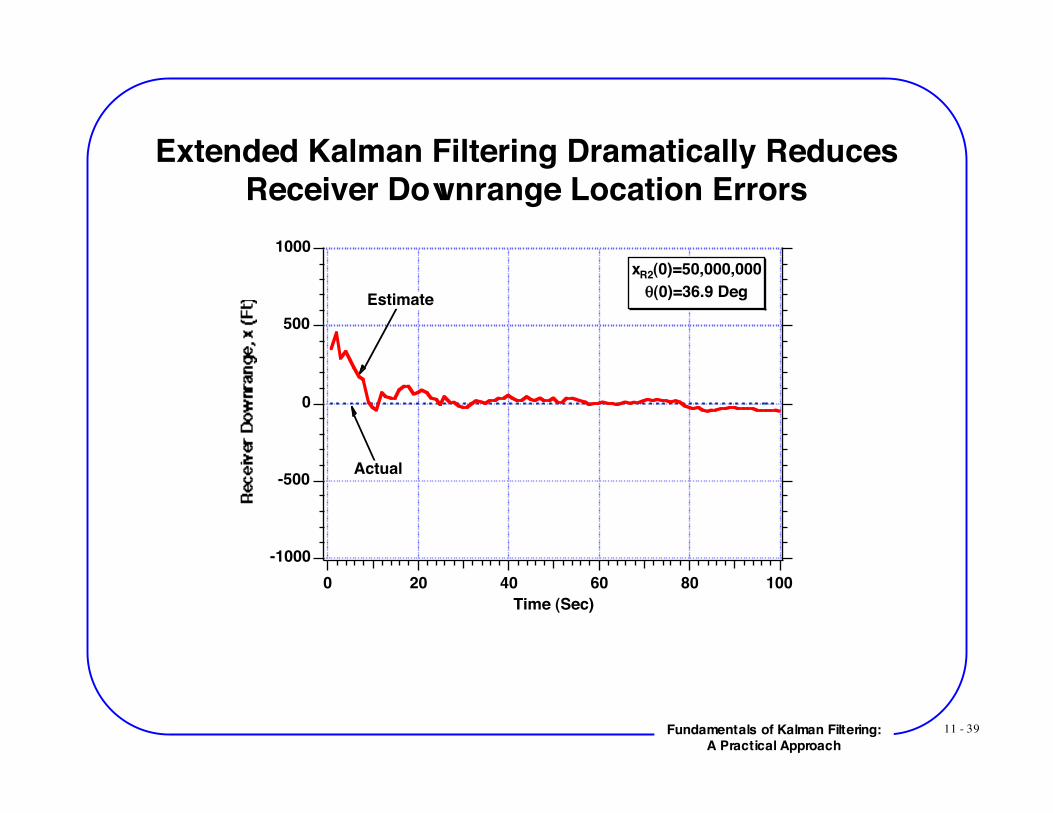
Extended Kalman Filtering Dramatically ReducesReceiver Downrange Location Errors
-1000
-500
0
500
1000
100806040200
Time (Sec)
xR2(0)=50,000,000
!(0)=36.9 Deg
Actual
Estimate
11 - 40Fundamentals of Kalman Filtering:A Practical Approach
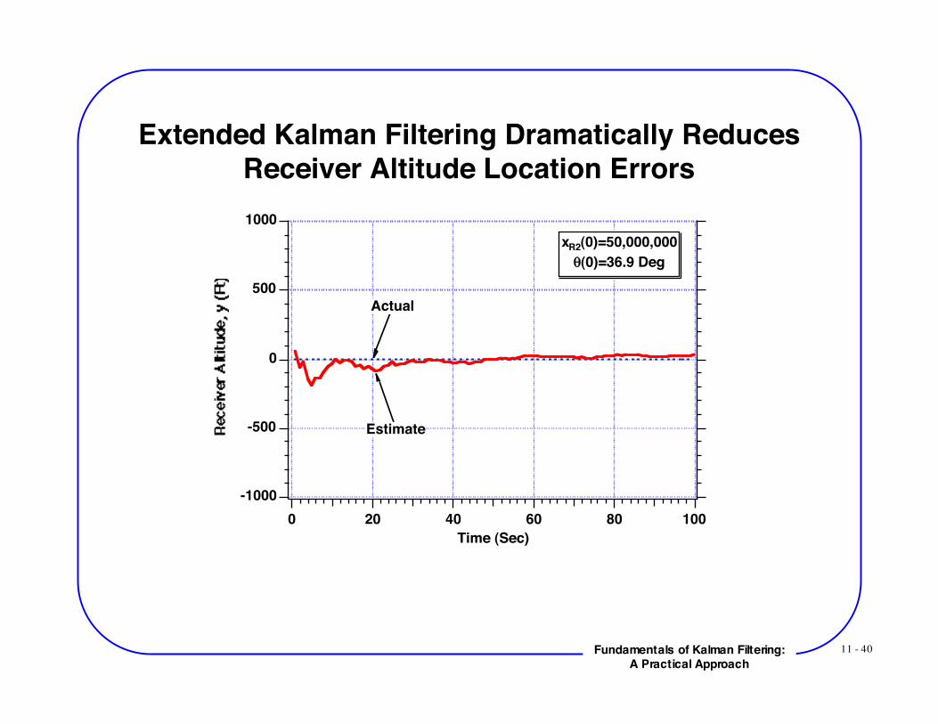
Extended Kalman Filtering Dramatically ReducesReceiver Altitude Location Errors
-1000
-500
0
500
1000
100806040200
Time (Sec)
xR2(0)=50,000,000
!(0)=36.9 Deg
Actual
Estimate
11 - 41Fundamentals of Kalman Filtering:A Practical Approach
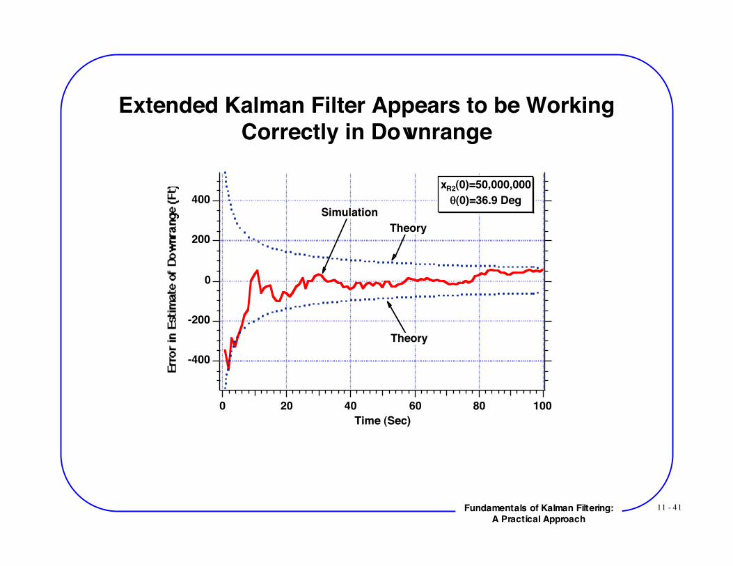
Extended Kalman Filter Appears to be WorkingCorrectly in Downrange
-400
-200
0
200
400
100806040200
Time (Sec)
xR2(0)=50,000,000
!(0)=36.9 DegSimulation
Theory
Theory
11 - 42Fundamentals of Kalman Filtering:A Practical Approach
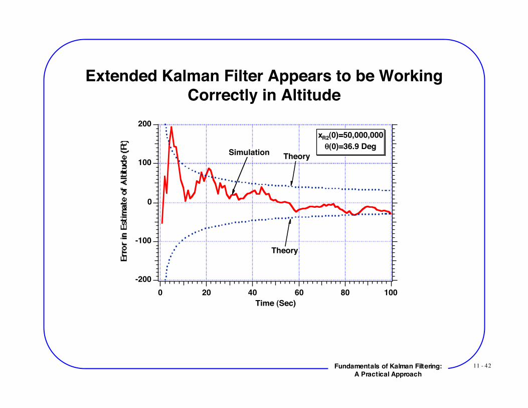
Extended Kalman Filter Appears to be WorkingCorrectly in Altitude
-200
-100
0
100
200
100806040200
Time (Sec)
xR2(0)=50,000,000
!(0)=36.9 DegSimulation
Theory
Theory
11 - 43Fundamentals of Kalman Filtering:A Practical Approach
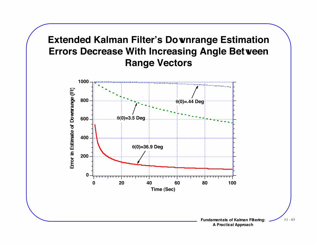
Extended Kalman Filter’s Downrange EstimationErrors Decrease With Increasing Angle Between
Range Vectors1000
800
600
400
200
0
100806040200
Time (Sec)
!(0)=.44 Deg
!(0)=3.5 Deg
!(0)=36.9 Deg

11 - 44Fundamentals of Kalman Filtering:A Practical Approach
Extended Kalman Filter’s Altitude Estimation ErrorsRemain Approximately Constant With Increasing
Angle Between Range Vectors
300
250
200
150
100
50
0
100806040200
Time (Sec)
!(0)=.44 Deg
!(0)=3.5 Deg
!(0)=36.9 Deg
11 - 45Fundamentals of Kalman Filtering:A Practical Approach
Using Extended Kalman Filtering With One Satellite
11 - 46Fundamentals of Kalman Filtering:A Practical Approach
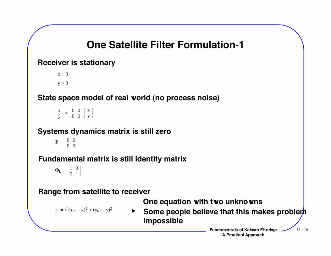
One Satellite Filter Formulation-1Receiver is stationary
x = 0
y = 0
State space model of real world (no process noise)x
y = 0 0
0 0
x
y
Systems dynamics matrix is still zeroF =
0 0
0 0
Fundamental matrix is still identity matrix!k =
1 0
0 1
Range from satellite to receiver
r1 = (xR1 - x)2 + (yR1 - y)2
One equation with two unknownsSome people believe that this makes problemimpossible

11 - 47Fundamentals of Kalman Filtering:A Practical Approach
One Satellite Filter Formulation-2
New linearized measurement equation!r1
* = "r1
"x
"r1
"y !x
!y +vr1
New measurement noise matrix is a scalarRk =!
r1
2
New linearized measurement matrixHk =
!r1
!x
!r1
!y
Evaluating partial derivatives
r1 = (xR1 - x)2 + (yR1 - y)2
!r1
!x = .5 (xR1-x)2+(yR1-y)2 -.5
2(xR1-x)(-1) = -(xR1-x)
r1
!r1
!y = .5 (xR1-x)2+(yR1-y)2 -.5
2(yR1-y)(-1) = -(yR1-y)
r1
Linearized measurement matrix
Hk = -(xR1-x)
r1 -(yR1-y)
r1
11 - 48Fundamentals of Kalman Filtering:A Practical Approach
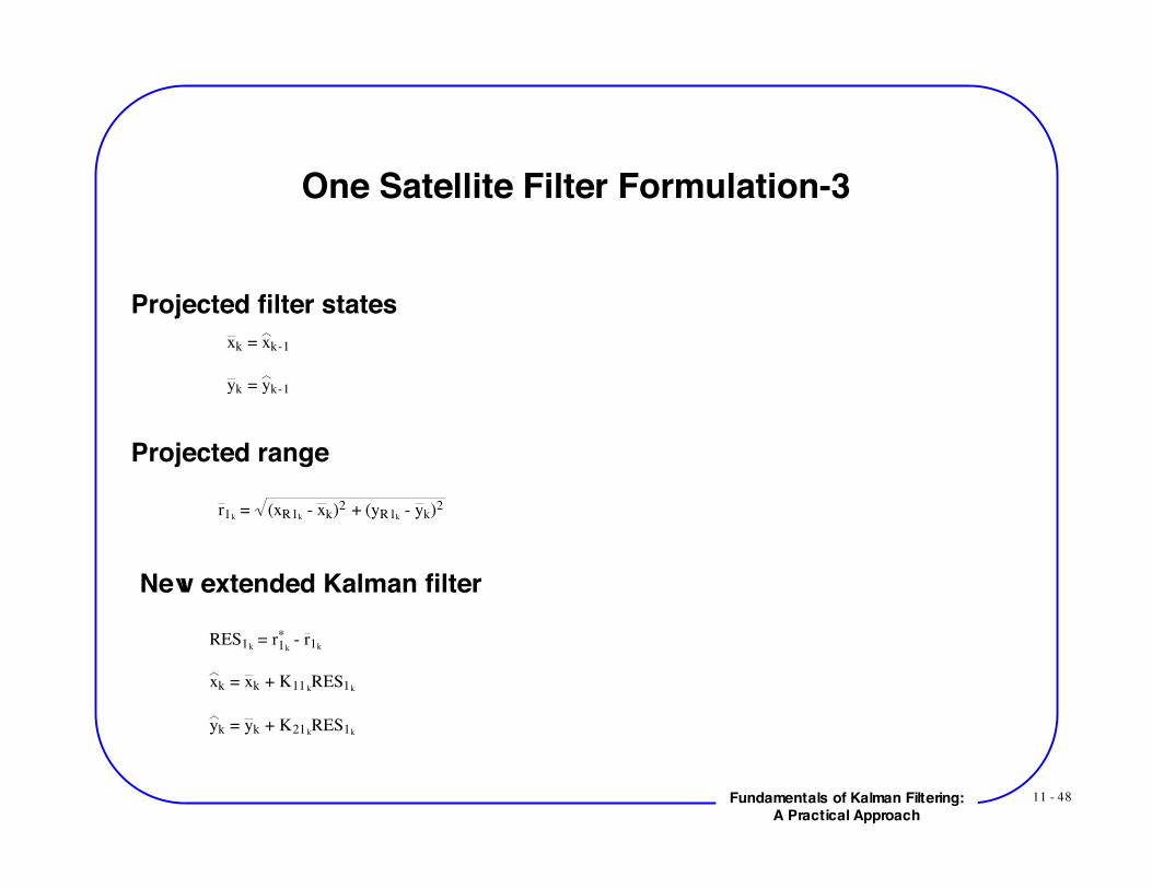
One Satellite Filter Formulation-3
Projected filter statesxk = xk-1
yk = yk-1
Projected range
r1k = (xR1k
- xk)2 + (yR1k - yk)2
New extended Kalman filter
RES1k = r1k
* - r1k
xk = xk + K11 kRES1k
yk = yk + K21kRES1k

11 - 49Fundamentals of Kalman Filtering:A Practical Approach
MATLAB Extended Kalman Filter for LocatingReceiver Based on Measurements From 1 Satellite-1
SIGNOISE=300.;X=0.;Y=0.;XH=1000.;YH=2000.;XR1=1000000.;YR1=20000.*3280.;ORDER=2;TS=1.;TF=100.;T=0.;S=0.;H=.01;PHI=zeros(ORDER,ORDER);P=zeros(ORDER,ORDER);IDNP=eye(ORDER);Q=zeros(ORDER,ORDER);P(1,1)=1000. 2̂;P(2,2)=2000. 2̂;RMAT(1,1)=SIGNOISE 2̂;count=0;while T<=TF
XR1OLD=XR1; XR1D=-14600.; XR1=XR1+H*XR1D; T=T+H;
XR1D=-14600.; XR1=.5*(XR1OLD+XR1+H*XR1D); S=S+H;
Initial estimate of receiver location
Initial covariance matrix
Integrate satellite equations usingsecond-order Runge-Kutta technique
11 - 50Fundamentals of Kalman Filtering:A Practical Approach
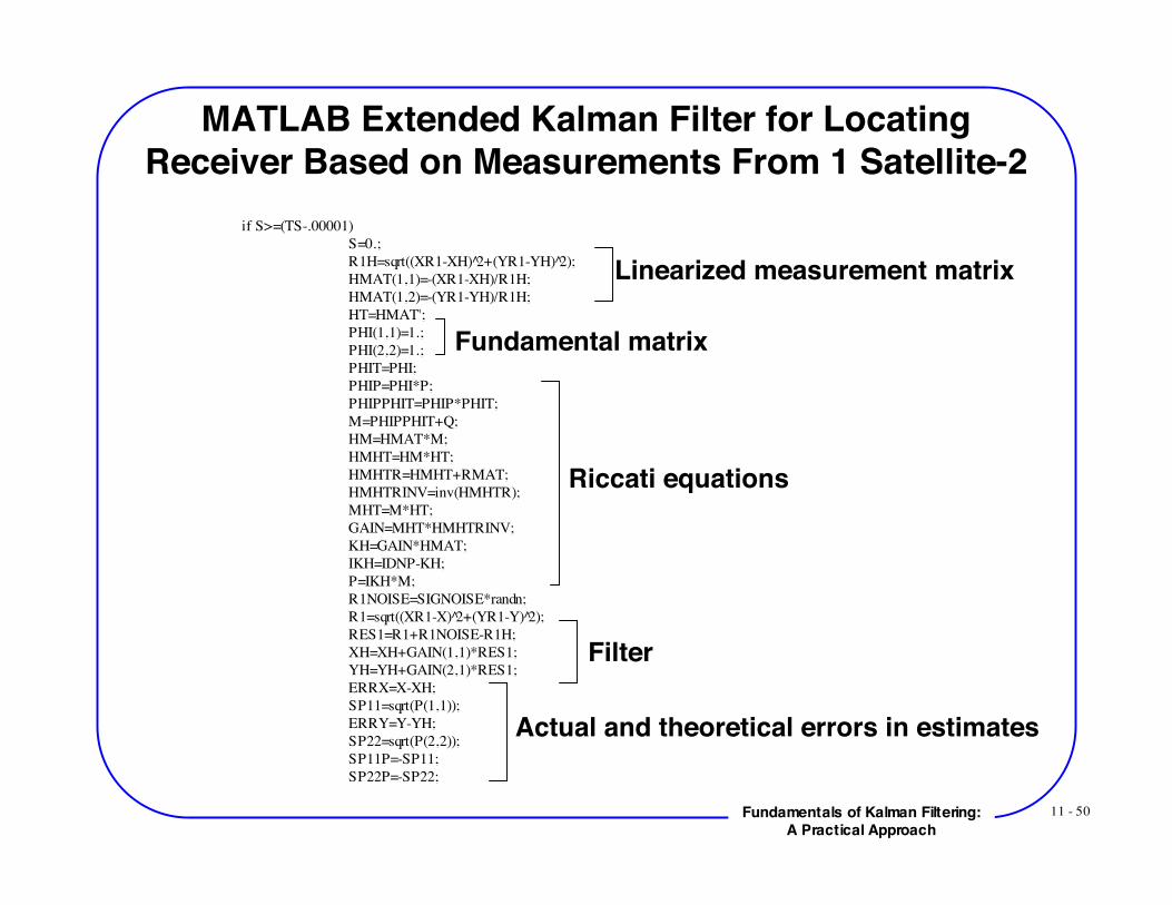
MATLAB Extended Kalman Filter for LocatingReceiver Based on Measurements From 1 Satellite-2
if S>=(TS-.00001)S=0.;R1H=sqrt((XR1-XH) 2̂+(YR1-YH) 2̂);HMAT(1,1)=-(XR1-XH)/R1H;HMAT(1,2)=-(YR1-YH)/R1H;HT=HMAT';PHI(1,1)=1.;PHI(2,2)=1.;PHIT=PHI;
PHIP=PHI*P; PHIPPHIT=PHIP*PHIT; M=PHIPPHIT+Q; HM=HMAT*M; HMHT=HM*HT; HMHTR=HMHT+RMAT;
HMHTRINV=inv(HMHTR);MHT=M*HT;
GAIN=MHT*HMHTRINV;KH=GAIN*HMAT;
IKH=IDNP-KH; P=IKH*M; R1NOISE=SIGNOISE*randn;
R1=sqrt((XR1-X) 2̂+(YR1-Y) 2̂);RES1=R1+R1NOISE-R1H;XH=XH+GAIN(1,1)*RES1;YH=YH+GAIN(2,1)*RES1;ERRX=X-XH;SP11=sqrt(P(1,1));ERRY=Y-YH;SP22=sqrt(P(2,2));SP11P=-SP11;SP22P=-SP22;
Linearized measurement matrix
Fundamental matrix
Riccati equations
Filter
Actual and theoretical errors in estimates
11 - 51Fundamentals of Kalman Filtering:A Practical Approach
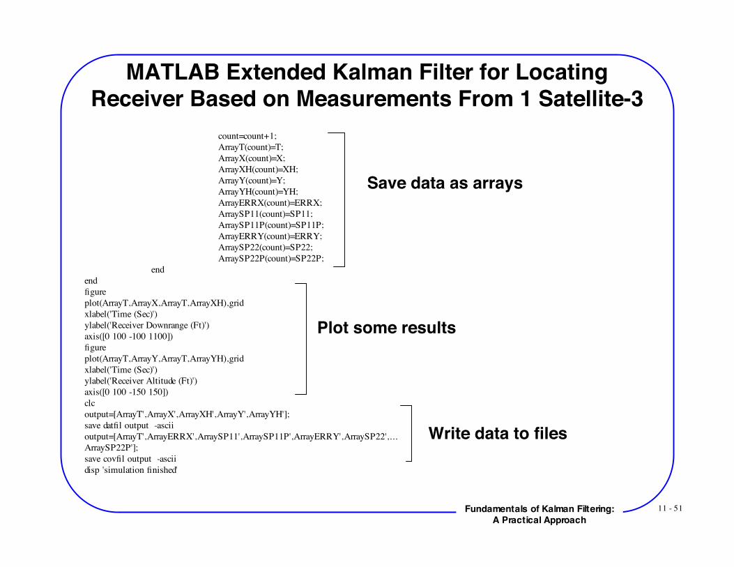
MATLAB Extended Kalman Filter for LocatingReceiver Based on Measurements From 1 Satellite-3
count=count+1;ArrayT(count)=T;ArrayX(count)=X;ArrayXH(count)=XH;ArrayY(count)=Y;ArrayYH(count)=YH;ArrayERRX(count)=ERRX;ArraySP11(count)=SP11;ArraySP11P(count)=SP11P;ArrayERRY(count)=ERRY;ArraySP22(count)=SP22;ArraySP22P(count)=SP22P;
endendfigureplot(ArrayT,ArrayX,ArrayT,ArrayXH),gridxlabel('Time (Sec)')ylabel('Receiver Downrange (Ft)')axis([0 100 -100 1100])figureplot(ArrayT,ArrayY,ArrayT,ArrayYH),gridxlabel('Time (Sec)')ylabel('Receiver Altitude (Ft)')axis([0 100 -150 150])clcoutput=[ArrayT',ArrayX',ArrayXH',ArrayY',ArrayYH'];save datfil output -asciioutput=[ArrayT',ArrayERRX',ArraySP11',ArraySP11P',ArrayERRY',ArraySP22',...ArraySP22P'];save covfil output -asciidisp 'simulation finished'
Save data as arrays
Plot some results
Write data to files
11 - 52Fundamentals of Kalman Filtering:A Practical Approach
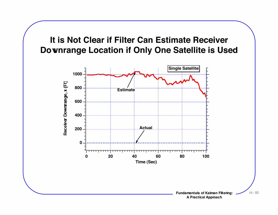
It is Not Clear if Filter Can Estimate ReceiverDownrange Location if Only One Satellite is Used
1000
800
600
400
200
0
100806040200
Time (Sec)
Single Satellite
Actual
Estimate
11 - 53Fundamentals of Kalman Filtering:A Practical Approach
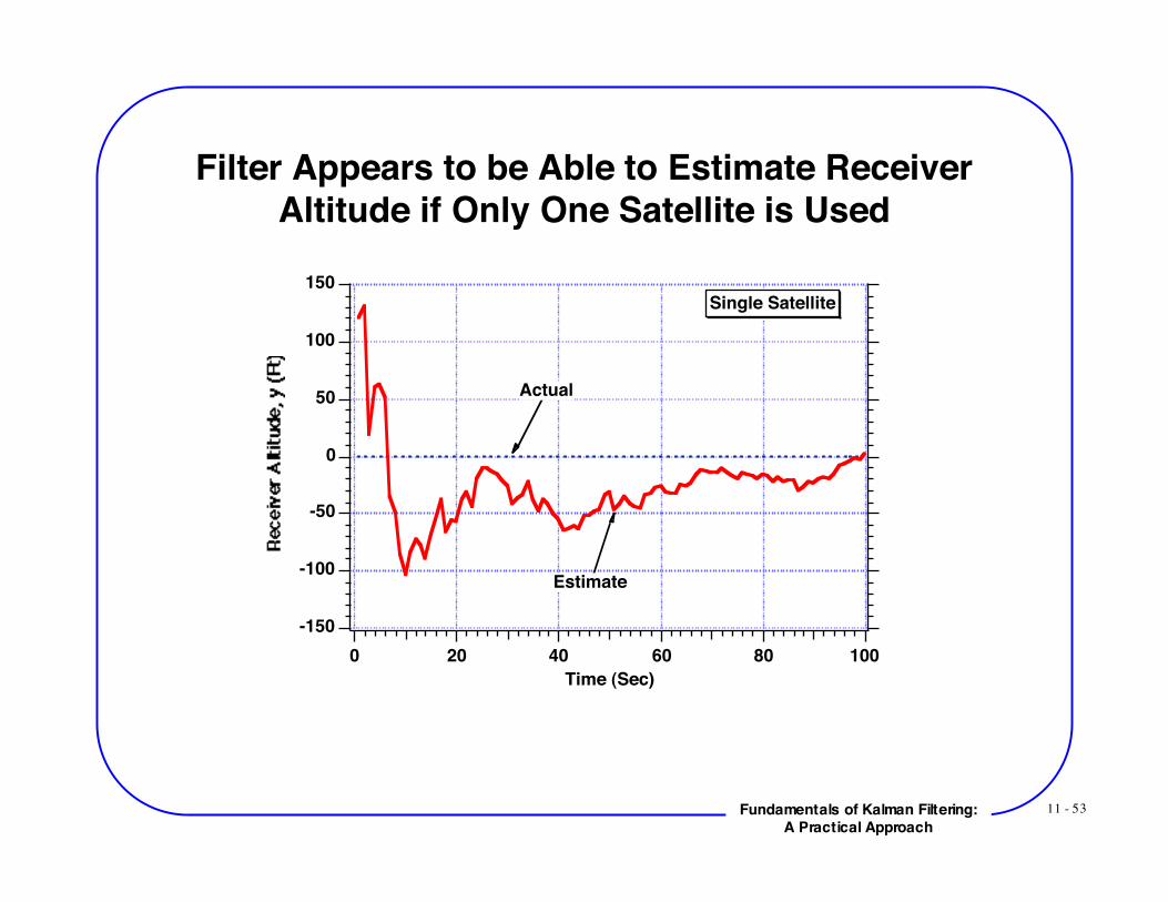
Filter Appears to be Able to Estimate ReceiverAltitude if Only One Satellite is Used
-150
-100
-50
0
50
100
150
100806040200
Time (Sec)
Single Satellite
Actual
Estimate
11 - 54Fundamentals of Kalman Filtering:A Practical Approach
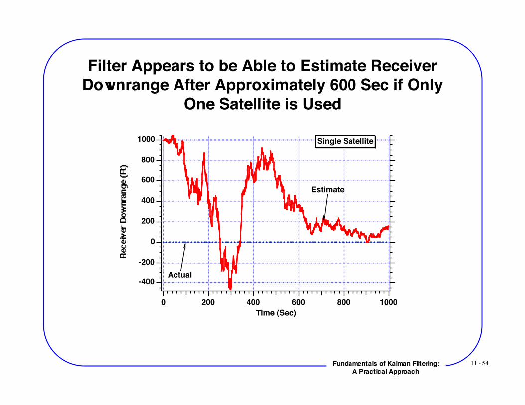
Filter Appears to be Able to Estimate ReceiverDownrange After Approximately 600 Sec if Only
One Satellite is Used
1000
800
600
400
200
0
-200
-400
10008006004002000
Time (Sec)
Single Satellite
Actual
Estimate
11 - 55Fundamentals of Kalman Filtering:A Practical Approach
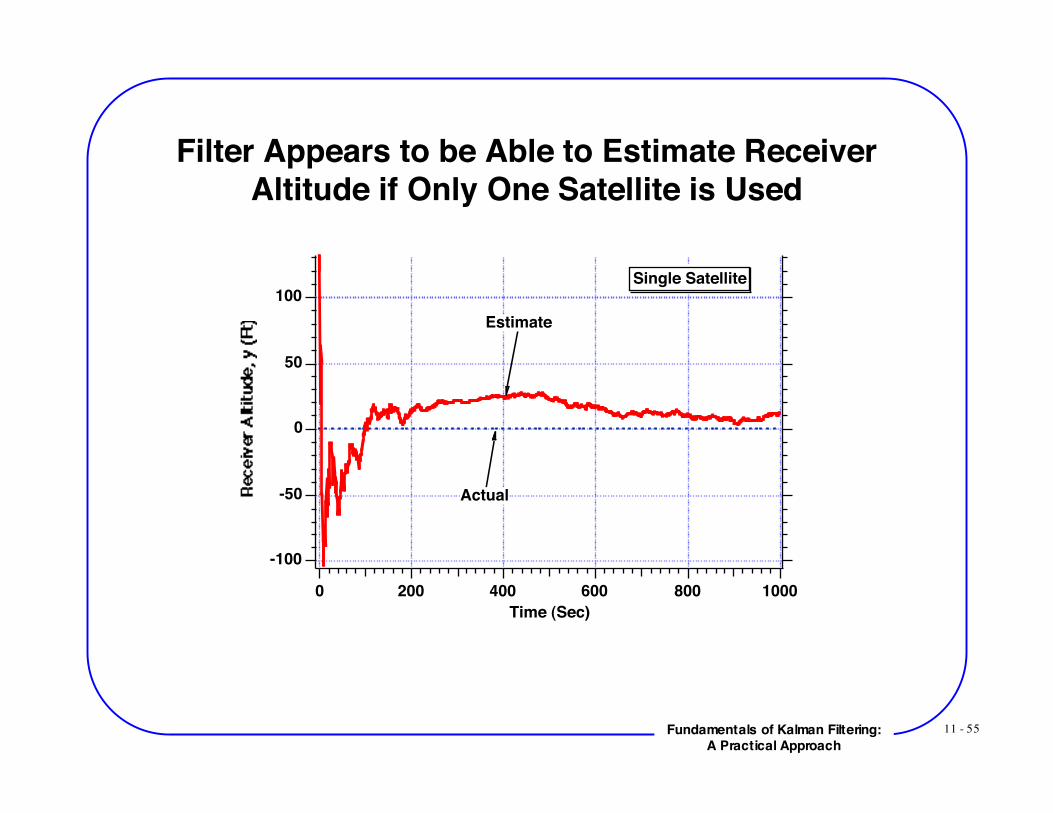
Filter Appears to be Able to Estimate ReceiverAltitude if Only One Satellite is Used
100
50
0
-50
-100
10008006004002000
Time (Sec)
Single Satellite
Actual
Estimate
11 - 56Fundamentals of Kalman Filtering:A Practical Approach
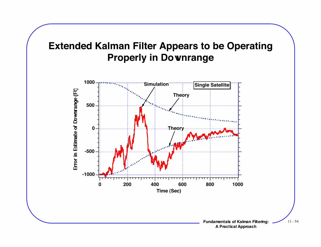
Extended Kalman Filter Appears to be OperatingProperly in Downrange
-1000
-500
0
500
1000
10008006004002000
Time (Sec)
Single SatelliteSimulation
Theory
Theory

11 - 57Fundamentals of Kalman Filtering:A Practical Approach
Extended Kalman Filter Appears to be OperatingProperly in Altitude
-100
-50
0
50
100
10008006004002000
Time (Sec)
Single Satellite
Simulation Theory
Theory
11 - 58Fundamentals of Kalman Filtering:A Practical Approach
Using Extended Kalman Filtering With ConstantVelocity Receiver

11 - 59Fundamentals of Kalman Filtering:A Practical Approach
Developing New Extended Kalman Filter-1Model of real world for moving receiver
x = us
y = us
Put model in state space formx
x
y
y
=
0 1 0 0
0 0 0 0
0 0 0 1
0 0 0 0
x
x
y
y
+
0
us
0
us
Continuous process noise matrix
Q =
0 0 0 0
0 !s 0 0
0 0 0 0
0 0 0 !s
Systems dynamics matrix
F =
0 1 0 0
0 0 0 0
0 0 0 1
0 0 0 0
11 - 60Fundamentals of Kalman Filtering:A Practical Approach
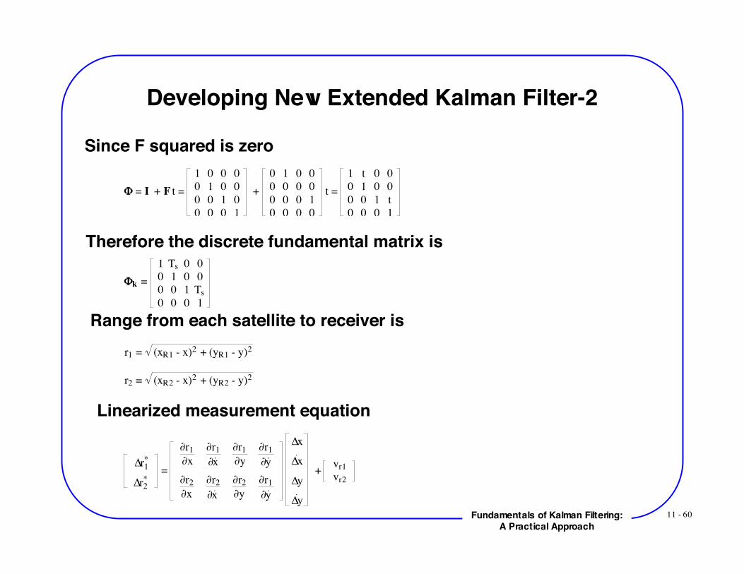
Developing New Extended Kalman Filter-2
Since F squared is zero
! = I + F t =
1 0 0 0
0 1 0 0
0 0 1 0
0 0 0 1
+
0 1 0 0
0 0 0 0
0 0 0 1
0 0 0 0
t =
1 t 0 0
0 1 0 0
0 0 1 t
0 0 0 1
Therefore the discrete fundamental matrix is
!k =
1 Ts 0 0
0 1 0 0
0 0 1 Ts
0 0 0 1
Range from each satellite to receiver isr1 = (xR1 - x)2 + (yR1 - y)2
r2 = (xR2 - x)2 + (yR2 - y)2
Linearized measurement equation
!r1*
!r2*
=
"r1
"x
"r1
"x
"r1
"y
"r1
"y
"r2
"x
"r2
"x
"r2
"y
"r1
"y
!x
!x
!y
!y
+ vr1
vr2
11 - 61Fundamentals of Kalman Filtering:A Practical Approach
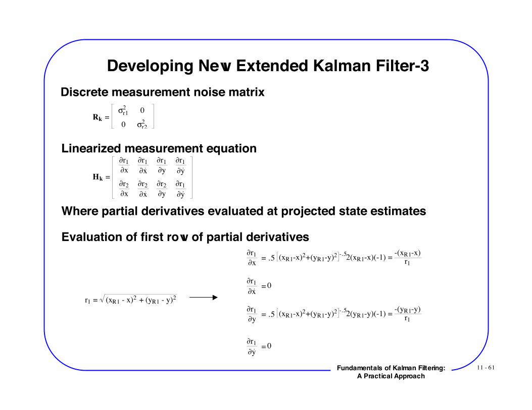
Developing New Extended Kalman Filter-3Discrete measurement noise matrix
Rk = !
r1
20
0 !r2
2
Linearized measurement equation
Hk =
!r1
!x
!r1
!x
!r1
!y
!r1
!y
!r2
!x
!r2
!x
!r2
!y
!r1
!y
Where partial derivatives evaluated at projected state estimates
Evaluation of first row of partial derivatives!r1
!x = .5 (xR1-x)2+(yR1-y)2 -.5
2(xR1-x)(-1) = -(xR1-x)
r1
r1 = (xR1 - x)2 + (yR1 - y)2
!r1
!x = 0
!r1
!y = .5 (xR1-x)2+(yR1-y)2 -.5
2(yR1-y)(-1) = -(yR1-y)
r1
!r1
!y = 0
11 - 62Fundamentals of Kalman Filtering:A Practical Approach
Developing New Extended Kalman Filter-4
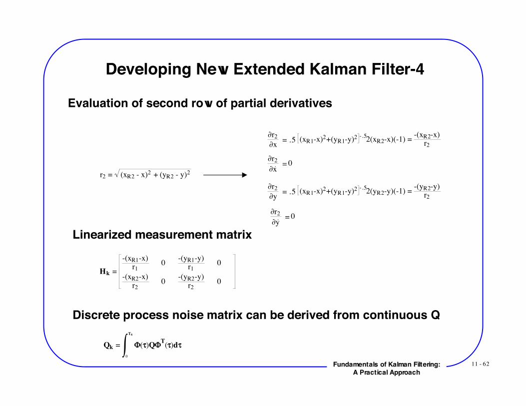
Evaluation of second row of partial derivatives
!r2
!x = .5 (xR1-x)2+(yR1-y)2 -.5
2(xR2-x)(-1) = -(xR2-x)
r2
!r2
!x = 0
!r2
!y = .5 (xR1-x)2+(yR1-y)2 -.5
2(yR2-y)(-1) = -(yR2-y)
r2
!r2
!y = 0
r2 = (xR2 - x)2 + (yR2 - y)2
Discrete process noise matrix can be derived from continuous Q
Qk = !(")Q!T(")d"
0
Ts
Linearized measurement matrix
Hk =
-(xR1-x)r1
0-(yR1-y)
r10
-(xR2-x)r2
0-(yR2-y)
r20
11 - 63Fundamentals of Kalman Filtering:A Practical Approach
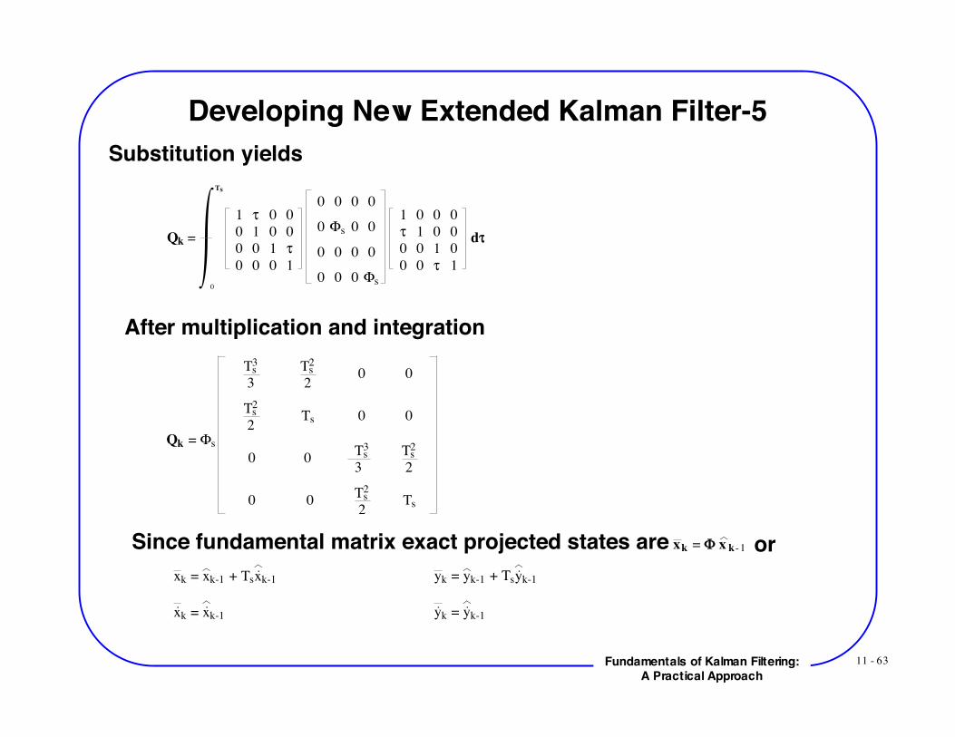
Developing New Extended Kalman Filter-5Substitution yields
Qk =
1 ! 0 0
0 1 0 0
0 0 1 !
0 0 0 1
0 0 0 0
0 "s 0 0
0 0 0 0
0 0 0 "s
1 0 0 0
! 1 0 0
0 0 1 0
0 0 ! 1
d!
0
Ts
After multiplication and integration
Qk = !s
Ts3
3
Ts2
2 0 0
Ts2
2 Ts 0 0
0 0 Ts
3
3
Ts2
2
0 0 Ts
2
2 Ts
Since fundamental matrix exact projected states arexk = xk-1 + Tsxk-1
xk = xk-1
yk = yk-1 + Tsyk-1
yk = yk-1
orxk = ! x k-1
11 - 64Fundamentals of Kalman Filtering:A Practical Approach
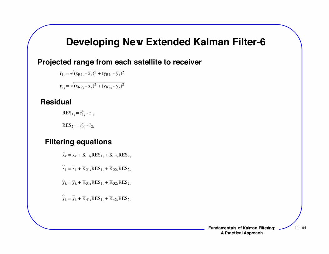
Developing New Extended Kalman Filter-6
Projected range from each satellite to receiverr1k
= (xR1k - xk)2 + (yR1k
- yk)2
r2k = (xR2k
- xk)2 + (yR2k - yk)2
ResidualRES1k
= r1k
* - r1k
RES2k = r2k
* - r2k
Filtering equationsxk = xk + K11k
RES1k + K12k
RES2k
xk = xk + K21kRES1k
+ K22kRES2k
yk = yk + K31kRES1k
+ K32kRES2k
yk = yk + K41kRES1k
+ K42 kRES2k
11 - 65Fundamentals of Kalman Filtering:A Practical Approach
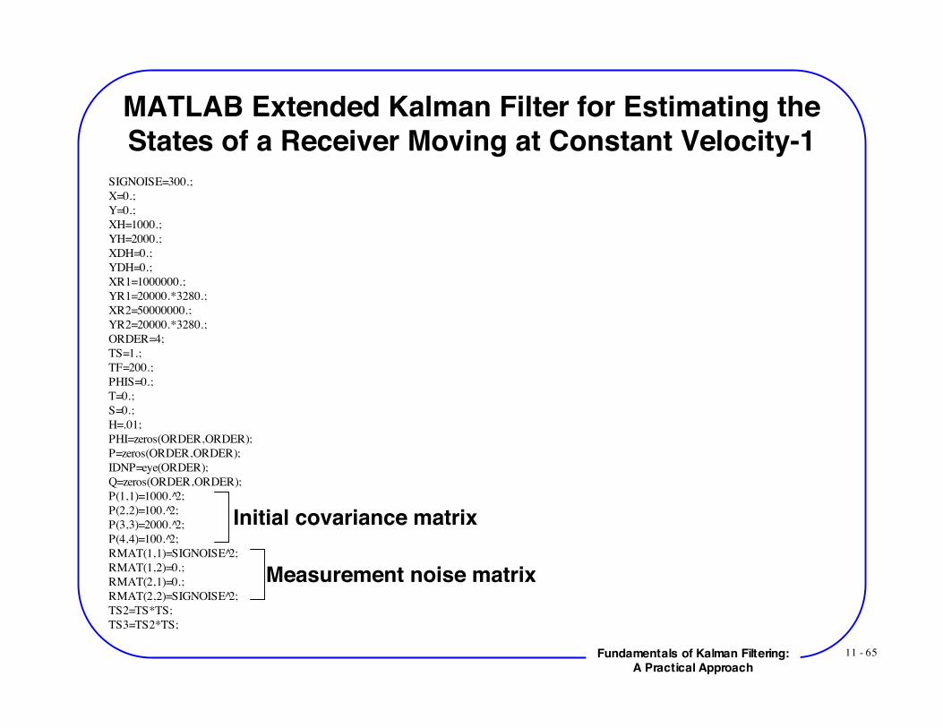
MATLAB Extended Kalman Filter for Estimating theStates of a Receiver Moving at Constant Velocity-1
SIGNOISE=300.;X=0.;Y=0.;XH=1000.;YH=2000.;XDH=0.;YDH=0.;XR1=1000000.;YR1=20000.*3280.;XR2=50000000.;YR2=20000.*3280.;ORDER=4;TS=1.;TF=200.;PHIS=0.;T=0.;S=0.;H=.01;PHI=zeros(ORDER,ORDER);P=zeros(ORDER,ORDER);IDNP=eye(ORDER);Q=zeros(ORDER,ORDER);P(1,1)=1000. 2̂;P(2,2)=100. 2̂;P(3,3)=2000. 2̂;P(4,4)=100. 2̂;RMAT(1,1)=SIGNOISE 2̂;RMAT(1,2)=0.;RMAT(2,1)=0.;RMAT(2,2)=SIGNOISE 2̂;TS2=TS*TS;TS3=TS2*TS;
Initial covariance matrix
Measurement noise matrix
11 - 66Fundamentals of Kalman Filtering:A Practical Approach
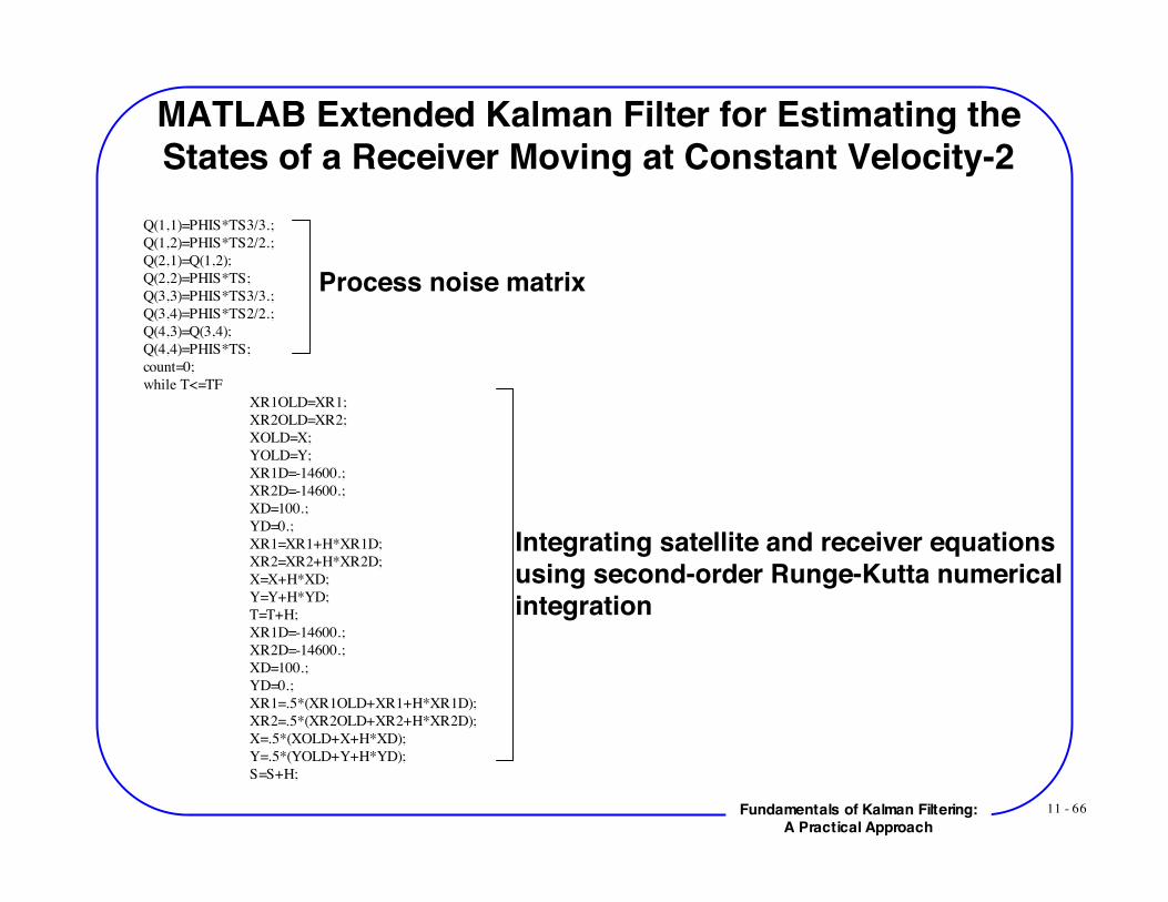
MATLAB Extended Kalman Filter for Estimating theStates of a Receiver Moving at Constant Velocity-2
Q(1,1)=PHIS*TS3/3.;Q(1,2)=PHIS*TS2/2.;Q(2,1)=Q(1,2);Q(2,2)=PHIS*TS;Q(3,3)=PHIS*TS3/3.;Q(3,4)=PHIS*TS2/2.;Q(4,3)=Q(3,4);Q(4,4)=PHIS*TS;count=0;while T<=TF
XR1OLD=XR1;XR2OLD=XR2;XOLD=X;YOLD=Y;
XR1D=-14600.;XR2D=-14600.;XD=100.;YD=0.;
XR1=XR1+H*XR1D;XR2=XR2+H*XR2D;X=X+H*XD;Y=Y+H*YD;
T=T+H;XR1D=-14600.;XR2D=-14600.;XD=100.;YD=0.;
XR1=.5*(XR1OLD+XR1+H*XR1D);XR2=.5*(XR2OLD+XR2+H*XR2D);X=.5*(XOLD+X+H*XD);Y=.5*(YOLD+Y+H*YD);
S=S+H;
Process noise matrix
Integrating satellite and receiver equationsusing second-order Runge-Kutta numericalintegration

11 - 67Fundamentals of Kalman Filtering:A Practical Approach
MATLAB Extended Kalman Filter for Estimating theStates of a Receiver Moving at Constant Velocity-3
if S>=(TS-.00001)S=0.;XB=XH+XDH*TS;YB=YH+YDH*TS;R1B=sqrt((XR1-XB) 2̂+(YR1-YB) 2̂);R2B=sqrt((XR2-XB) 2̂+(YR2-YB) 2̂);HMAT(1,1)=-(XR1-XB)/R1B;HMAT(1,2)=0.;HMAT(1,3)=-(YR1-YB)/R1B;HMAT(1,4)=0.;HMAT(2,1)=-(XR2-XB)/R2B;HMAT(2,2)=0.;HMAT(2,3)=-(YR2-YB)/R2B;HMAT(2,4)=0.;HT=HMAT';PHI(1,1)=1.;PHI(1,2)=TS;PHI(2,2)=1.;PHI(3,3)=1.;PHI(3,4)=TS;PHI(4,4)=1.;PHIT=PHI';
PHIP=PHI*P; PHIPPHIT=PHIP*PHIT; M=PHIPPHIT+Q; HM=HMAT*M; HMHT=HM*HT; HMHTR=HMHT+RMAT;
HMHTRINV=inv(HMHTR);MHT=M*HT;
GAIN=MHT*HMHTRINV;KH=GAIN*HMAT;
IKH=IDNP-KH; P=IKH*M;
R1NOISE=SIGNOISE*randn; R2NOISE=SIGNOISE*randn;
R1=sqrt((XR1-X) 2̂+(YR1-Y) 2̂);R2=sqrt((XR2-X) 2̂+(YR2-Y) 2̂);
Linearized measurement matrix
Fundamental matrix
Riccati equations
11 - 68Fundamentals of Kalman Filtering:A Practical Approach
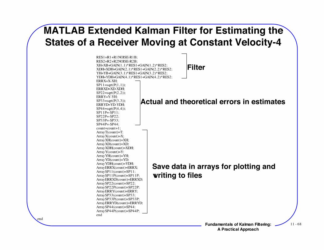
MATLAB Extended Kalman Filter for Estimating theStates of a Receiver Moving at Constant Velocity-4
RES1=R1+R1NOISE-R1B;RES2=R2+R2NOISE-R2B;XH=XB+GAIN(1,1)*RES1+GAIN(1,2)*RES2;XDH=XDH+GAIN(2,1)*RES1+GAIN(2,2)*RES2;YH=YB+GAIN(3,1)*RES1+GAIN(3,2)*RES2;YDH=YDH+GAIN(4,1)*RES1+GAIN(4,2)*RES2;ERRX=X-XH;SP11=sqrt(P(1,1));ERRXD=XD-XDH;SP22=sqrt(P(2,2));ERRY=Y-YH;SP33=sqrt(P(3,3));ERRYD=YD-YDH;SP44=sqrt(P(4,4));SP11P=-SP11;SP22P=-SP22;SP33P=-SP33;SP44P=-SP44;count=count+1;ArrayT(count)=T;ArrayX(count)=X;ArrayXH(count)=XH;ArrayXD(count)=XD;ArrayXDH(count)=XDH;ArrayY(count)=Y;ArrayYH(count)=YH;ArrayYD(count)=YD;ArrayYDH(count)=YDH;ArrayERRX(count)=ERRX;ArraySP11(count)=SP11;ArraySP11P(count)=SP11P;ArrayERRXD(count)=ERRXD;ArraySP22(count)=SP22;ArraySP22P(count)=SP22P;ArrayERRY(count)=ERRY;ArraySP33(count)=SP33;ArraySP33P(count)=SP33P;ArrayERRYD(count)=ERRYD;ArraySP44(count)=SP44;ArraySP44P(count)=SP44P;end
end
Filter
Actual and theoretical errors in estimates
Save data in arrays for plotting andwriting to files
11 - 69Fundamentals of Kalman Filtering:A Practical Approach
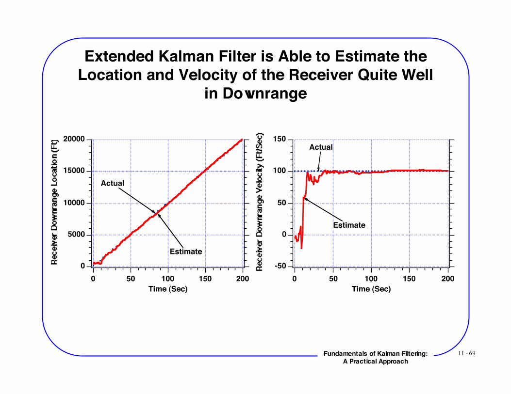
Extended Kalman Filter is Able to Estimate theLocation and Velocity of the Receiver Quite Well
in Downrange
20000
15000
10000
5000
0
200150100500
Time (Sec)
Actual
Estimate
150
100
50
0
-50
200150100500
Time (Sec)
Actual
Estimate
11 - 70Fundamentals of Kalman Filtering:A Practical Approach
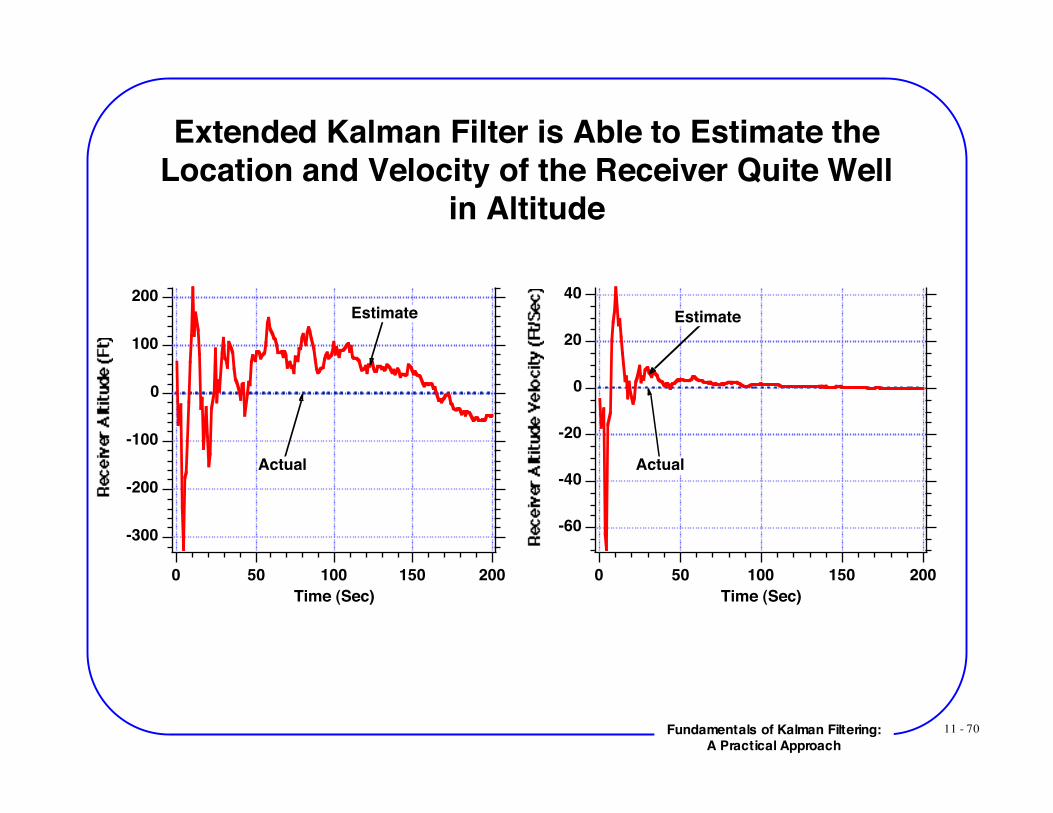
Extended Kalman Filter is Able to Estimate theLocation and Velocity of the Receiver Quite Well
in Altitude
-300
-200
-100
0
100
200
200150100500
Time (Sec)
Actual
Estimate
-60
-40
-20
0
20
40
200150100500
Time (Sec)
Actual
Estimate

11 - 71Fundamentals of Kalman Filtering:A Practical Approach
New Extended Kalman Filter Appears to beOperating Properly in Downrange
400
200
0
-200
-400
200150100500
Time (Sec)
Two SatellitesMoving Receiver
SimulationTheory
Theory
-20
-10
0
10
20
200150100500
Time (Sec)
Two SatellitesMoving Receiver
Simulation
Theory
Theory
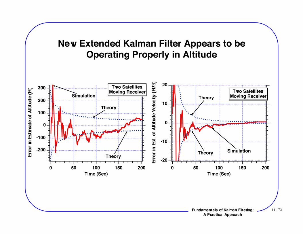
11 - 72Fundamentals of Kalman Filtering:A Practical Approach
New Extended Kalman Filter Appears to beOperating Properly in Altitude
300
200
100
0
-100
-200
200150100500
Time (Sec)
Two SatellitesMoving Receiver
Simulation
Theory
Theory-20
-10
0
10
20
200150100500
Time (Sec)
Two SatellitesMoving Receiver
Simulation
Theory
Theory
11 - 73Fundamentals of Kalman Filtering:A Practical Approach
Single Satellite With Constant Velocity Receiver
11 - 74Fundamentals of Kalman Filtering:A Practical Approach
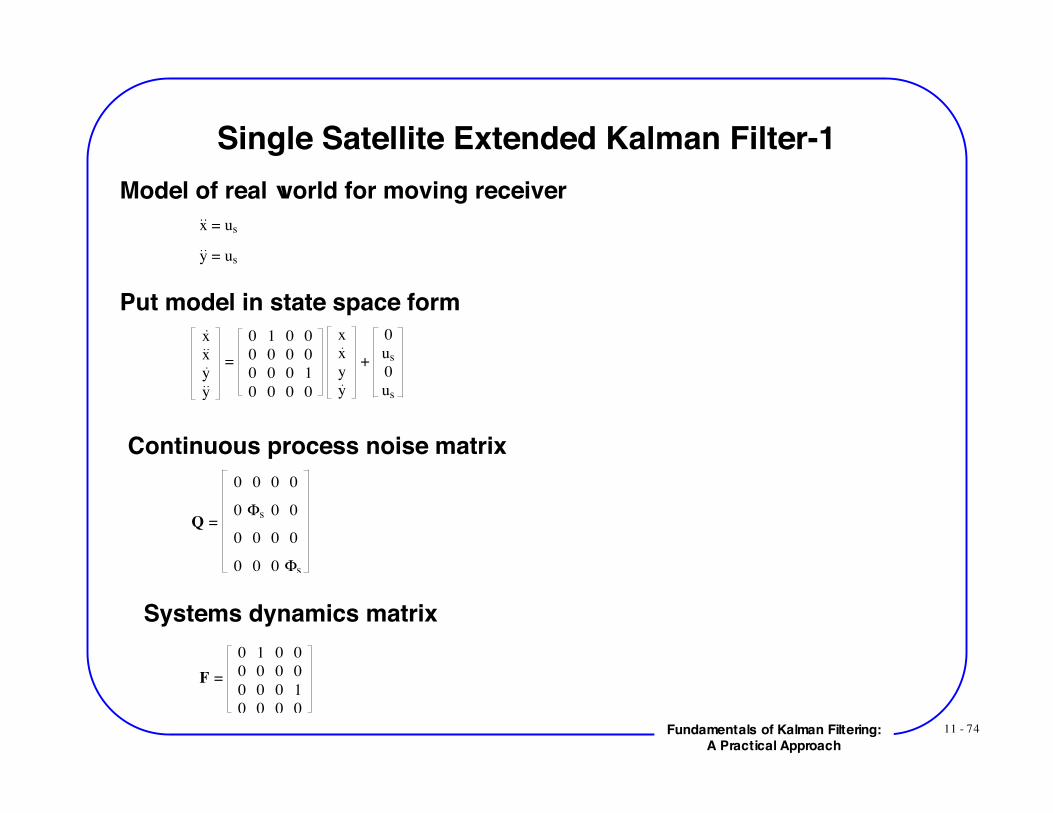
Single Satellite Extended Kalman Filter-1Model of real world for moving receiver
x = us
y = us
Put model in state space formx
x
y
y
=
0 1 0 0
0 0 0 0
0 0 0 1
0 0 0 0
x
x
y
y
+
0
us
0
us
Continuous process noise matrix
Q =
0 0 0 0
0 !s 0 0
0 0 0 0
0 0 0 !s
Systems dynamics matrix
F =
0 1 0 0
0 0 0 0
0 0 0 1
0 0 0 0
11 - 75Fundamentals of Kalman Filtering:A Practical Approach
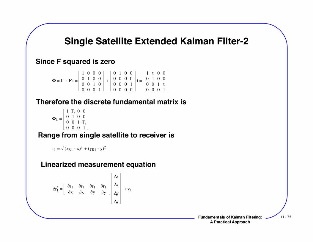
Single Satellite Extended Kalman Filter-2
Since F squared is zero
! = I + F t =
1 0 0 0
0 1 0 0
0 0 1 0
0 0 0 1
+
0 1 0 0
0 0 0 0
0 0 0 1
0 0 0 0
t =
1 t 0 0
0 1 0 0
0 0 1 t
0 0 0 1
Therefore the discrete fundamental matrix is
!k =
1 Ts 0 0
0 1 0 0
0 0 1 Ts
0 0 0 1
Range from single satellite to receiver isr1 = (xR1 - x)2 + (yR1 - y)2
Linearized measurement equation
!r1* =
"r1
"x
"r1
"x
"r1
"y
"r1
"y
!x
!x
!y
!y
+ vr1

11 - 76Fundamentals of Kalman Filtering:A Practical Approach
Single Satellite Extended Kalman Filter-3Discrete measurement noise matrix is now a scalar
Linearized measurement equation
Where partial derivatives evaluated at projected state estimates
Evaluation of partial derivatives!r1
!x = .5 (xR1-x)2+(yR1-y)2 -.5
2(xR1-x)(-1) = -(xR1-x)
r1
r1 = (xR1 - x)2 + (yR1 - y)2
!r1
!x = 0
!r1
!y = .5 (xR1-x)2+(yR1-y)2 -.5
2(yR1-y)(-1) = -(yR1-y)
r1
!r1
!y = 0
Rk =!r1
2
Hk =!r1
!x
!r1
!x
!r1
!y
!r1
!y
11 - 77Fundamentals of Kalman Filtering:A Practical Approach
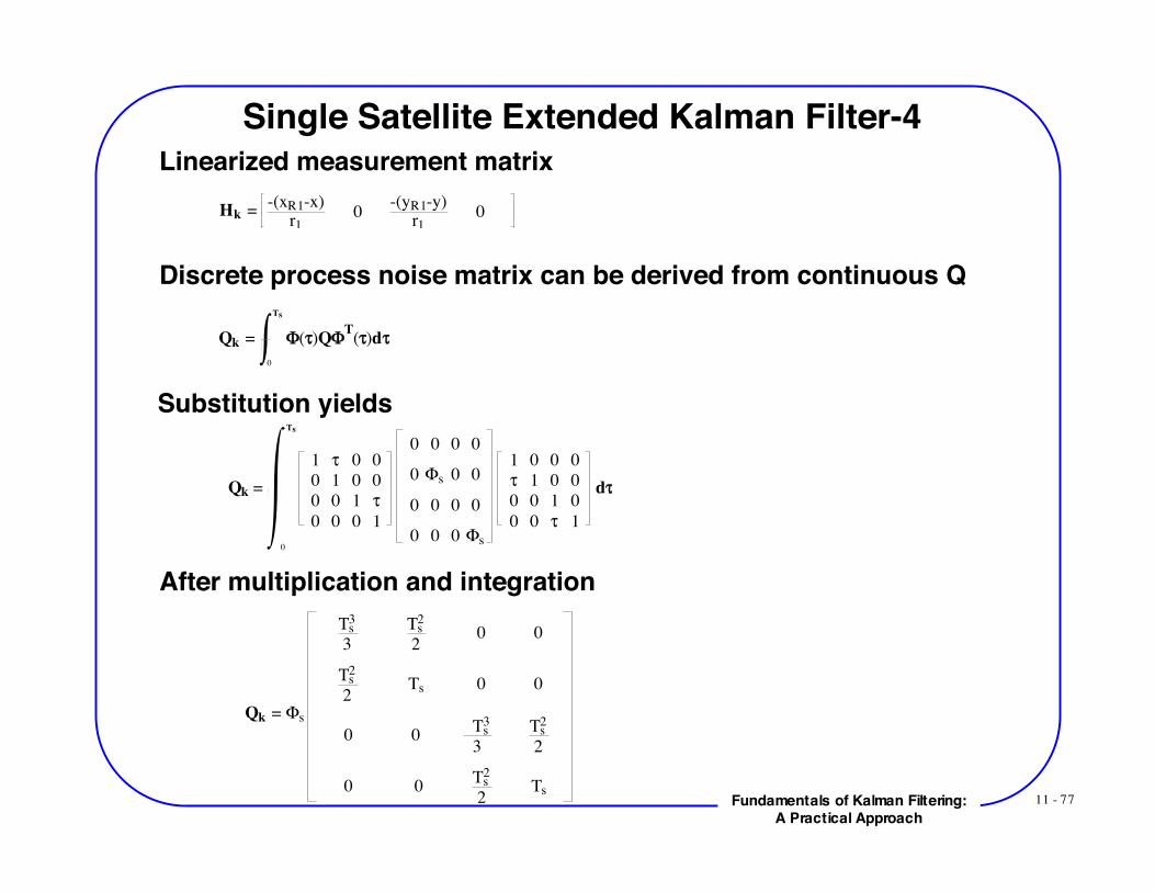
Single Satellite Extended Kalman Filter-4
Discrete process noise matrix can be derived from continuous Q
Qk = !(")Q!T(")d"
0
Ts
Linearized measurement matrixHk =
-(xR1-x)r1
0-(yR1-y)
r10
Substitution yields
Qk =
1 ! 0 0
0 1 0 0
0 0 1 !
0 0 0 1
0 0 0 0
0 "s 0 0
0 0 0 0
0 0 0 "s
1 0 0 0
! 1 0 0
0 0 1 0
0 0 ! 1
d!
0
Ts
After multiplication and integration
Qk = !s
Ts3
3
Ts2
2 0 0
Ts2
2 Ts 0 0
0 0 Ts
3
3
Ts2
2
0 0 Ts
2
2 Ts

11 - 78Fundamentals of Kalman Filtering:A Practical Approach
Single Satellite Extended Kalman Filter-5Project states ahead with exact fundamental matrix
xk = xk-1 + Tsxk-1
xk = xk-1
yk = yk-1 + Tsyk-1
yk = yk-1
Projected range from satellite to receiverr1k
= (xR1k - xk)2 + (yR1k
- yk)2
Extended Kalman filtering equationsRES1k
= r1k
* - r1k
xk = xk + K11kRES1k
xk = xk + K21kRES1k
yk = yk + K31kRES1k
yk = yk + K41kRES1k
orxk = ! x k-1
11 - 79Fundamentals of Kalman Filtering:A Practical Approach
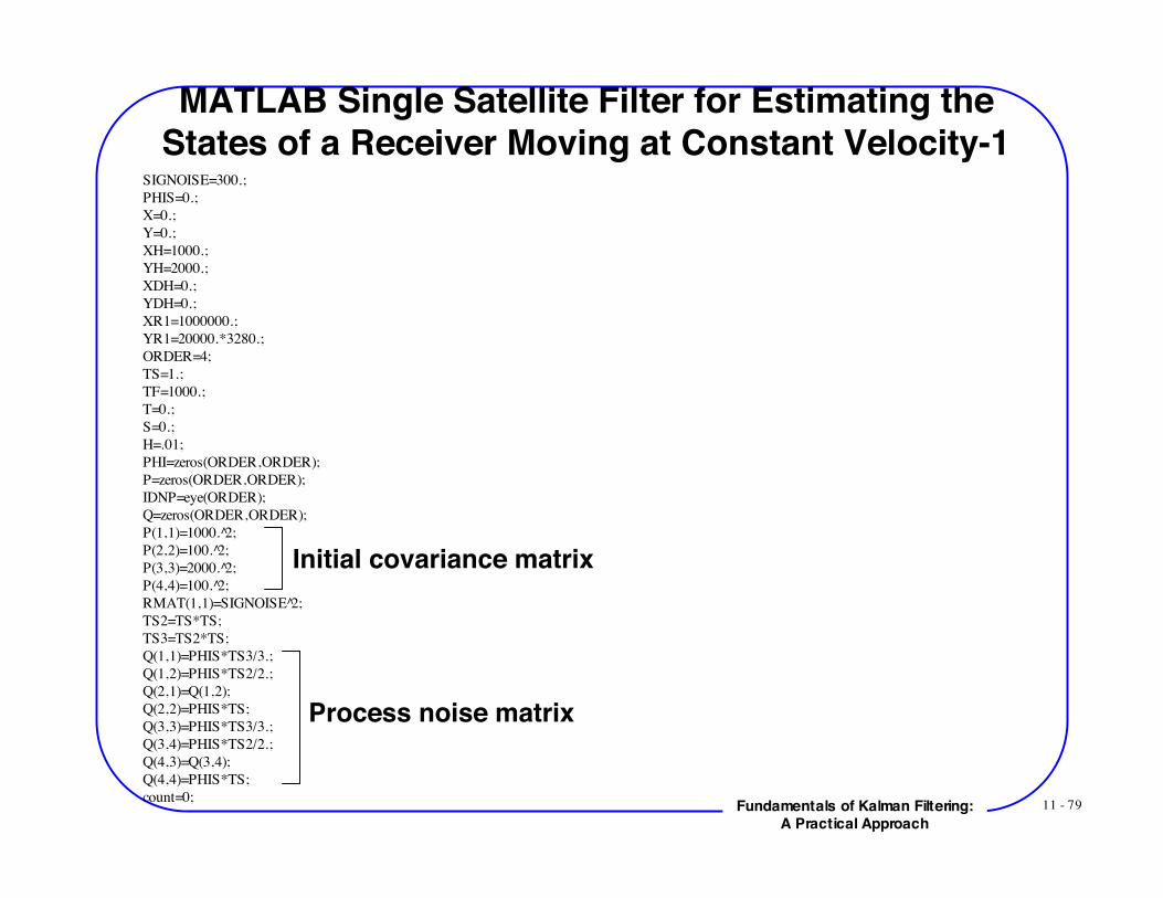
MATLAB Single Satellite Filter for Estimating theStates of a Receiver Moving at Constant Velocity-1
SIGNOISE=300.;PHIS=0.;X=0.;Y=0.;XH=1000.;YH=2000.;XDH=0.;YDH=0.;XR1=1000000.;YR1=20000.*3280.;ORDER=4;TS=1.;TF=1000.;T=0.;S=0.;H=.01;PHI=zeros(ORDER,ORDER);P=zeros(ORDER,ORDER);IDNP=eye(ORDER);Q=zeros(ORDER,ORDER);P(1,1)=1000. 2̂;P(2,2)=100. 2̂;P(3,3)=2000. 2̂;P(4,4)=100. 2̂;RMAT(1,1)=SIGNOISE 2̂;TS2=TS*TS;TS3=TS2*TS;Q(1,1)=PHIS*TS3/3.;Q(1,2)=PHIS*TS2/2.;Q(2,1)=Q(1,2);Q(2,2)=PHIS*TS;Q(3,3)=PHIS*TS3/3.;Q(3,4)=PHIS*TS2/2.;Q(4,3)=Q(3,4);Q(4,4)=PHIS*TS;count=0;
Initial covariance matrix
Process noise matrix

11 - 80Fundamentals of Kalman Filtering:A Practical Approach
MATLAB Single Satellite Filter for Estimating theStates of a Receiver Moving at Constant Velocity-2
while T<=TFXR1OLD=XR1;XOLD=X;YOLD=Y;
XR1D=-14600.;XD=100.;YD=0.;
XR1=XR1+H*XR1D;X=X+H*XD;Y=Y+H*YD;
T=T+H;XR1D=-14600.;XD=100.;YD=0.;
XR1=.5*(XR1OLD+XR1+H*XR1D);X=.5*(XOLD+X+H*XD);Y=.5*(YOLD+Y+H*YD);
S=S+H;if S>=(TS-.00001)
S=0.;XB=XH+XDH*TS;YB=YH+YDH*TS;R1B=sqrt((XR1-XB) 2̂+(YR1-YB) 2̂);HMAT(1,1)=-(XR1-XB)/R1B;HMAT(1,2)=0.;HMAT(1,3)=-(YR1-YB)/R1B;HMAT(1,4)=0.;HT=HMAT';PHI(1,1)=1.;PHI(1,2)=TS;PHI(2,2)=1.;PHI(3,3)=1.;PHI(3,4)=TS;PHI(4,4)=1.;PHIT=PHI';
Integrating satellite and receiver equationsUsing second-order Runge-Kutta technique
Linearized measurement matrix
Fundamental matrix

11 - 81Fundamentals of Kalman Filtering:A Practical Approach
MATLAB Single Satellite Filter for Estimating theStates of a Receiver Moving at Constant Velocity-3
PHIP=PHI*P; PHIPPHIT=PHIP*PHIT; M=PHIPPHIT+Q; HM=HMAT*M; HMHT=HM*HT; HMHTR=HMHT+RMAT;
HMHTRINV(1,1)=1./HMHTR(1,1);MHT=M*HT;
GAIN=MHT*HMHTRINV;KH=GAIN*HMAT;
IKH=IDNP-KH; P=IKH*M; R1NOISE=SIGNOISE*randn;
R1=sqrt((XR1-X) 2̂+(YR1-Y) 2̂);RES1=R1+R1NOISE-R1B;XH=XB+GAIN(1,1)*RES1;XDH=XDH+GAIN(2,1)*RES1;YH=YB+GAIN(3,1)*RES1;YDH=YDH+GAIN(4,1)*RES1;ERRX=X-XH;SP11=sqrt(P(1,1));ERRXD=XD-XDH;SP22=sqrt(P(2,2));ERRY=Y-YH;SP33=sqrt(P(3,3));ERRYD=YD-YDH;SP44=sqrt(P(4,4));SP11P=-SP11;SP22P=-SP22;SP33P=-SP33;SP44P=-SP44;count=count+1;
Riccati equations
Filter
Actual and theoretical errors in estimates

11 - 82Fundamentals of Kalman Filtering:A Practical Approach
MATLAB Single Satellite Filter for Estimating theStates of a Receiver Moving at Constant Velocity-4
ArrayT(count)=T;ArrayX(count)=X;ArrayXH(count)=XH;ArrayXD(count)=XD;ArrayXDH(count)=XDH;ArrayY(count)=Y;ArrayYH(count)=YH;ArrayYD(count)=YD;ArrayYDH(count)=YDH;ArrayERRX(count)=ERRX;ArraySP11(count)=SP11;ArraySP11P(count)=SP11P;ArrayERRXD(count)=ERRXD;ArraySP22(count)=SP22;ArraySP22P(count)=SP22P;ArrayERRY(count)=ERRY;ArraySP33(count)=SP33;ArraySP33P(count)=SP33P;ArrayERRYD(count)=ERRYD;ArraySP44(count)=SP44;ArraySP44P(count)=SP44P;
endendfigureplot(ArrayT,ArrayERRX,ArrayT,ArraySP11,ArrayT,ArraySP11P),gridxlabel('Time (Sec)')ylabel('Error in Estimate of Downrange (Ft)')axis([0 1000 -11000 11000])figureplot(ArrayT,ArrayERRXD,ArrayT,ArraySP22,ArrayT,ArraySP22P),gridxlabel('Time (Sec)')ylabel('Error in Estimate of Downrange Velocity (Ft/Sec)')axis([0 1000 -20 20])
Save data as arrays for plotting andwriting to files
Sample plots

11 - 83Fundamentals of Kalman Filtering:A Practical Approach
New Extended Kalman Filter Appears to beOperating Properly in Downrange
10000
5000
0
-5000
-10000
10008006004002000
Time (Sec)
One SatelliteMoving ReceiverSimulation
Theory
Theory
-20
-10
0
10
20
10008006004002000
Time (Sec)
Simulation
Theory
Theory
One SatelliteMoving Receiver
11 - 84Fundamentals of Kalman Filtering:A Practical Approach
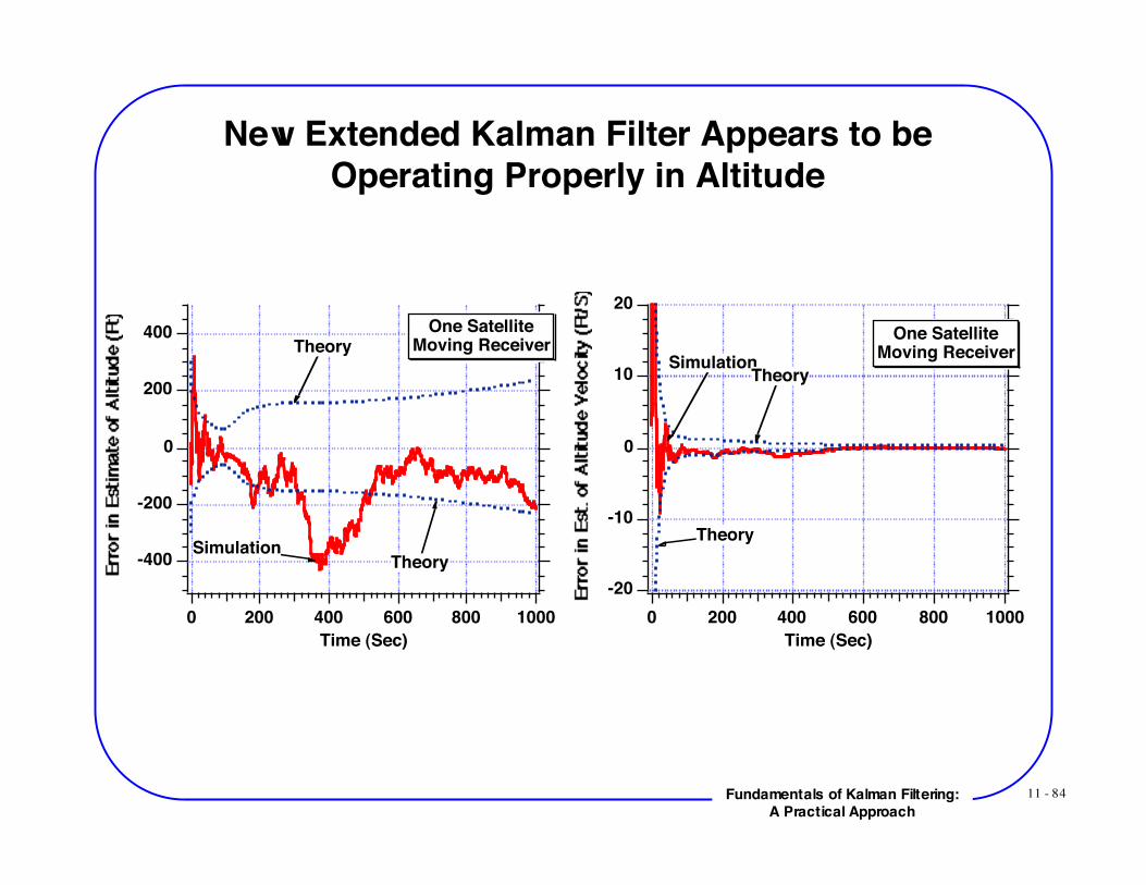
New Extended Kalman Filter Appears to beOperating Properly in Altitude
-400
-200
0
200
400
10008006004002000
Time (Sec)
Simulation
Theory
Theory
One SatelliteMoving Receiver
-20
-10
0
10
20
10008006004002000
Time (Sec)
SimulationTheory
Theory
One SatelliteMoving Receiver
11 - 85Fundamentals of Kalman Filtering:A Practical Approach
Using Extended Kalman Filtering With VariableVelocity Receiver
11 - 86Fundamentals of Kalman Filtering:A Practical Approach
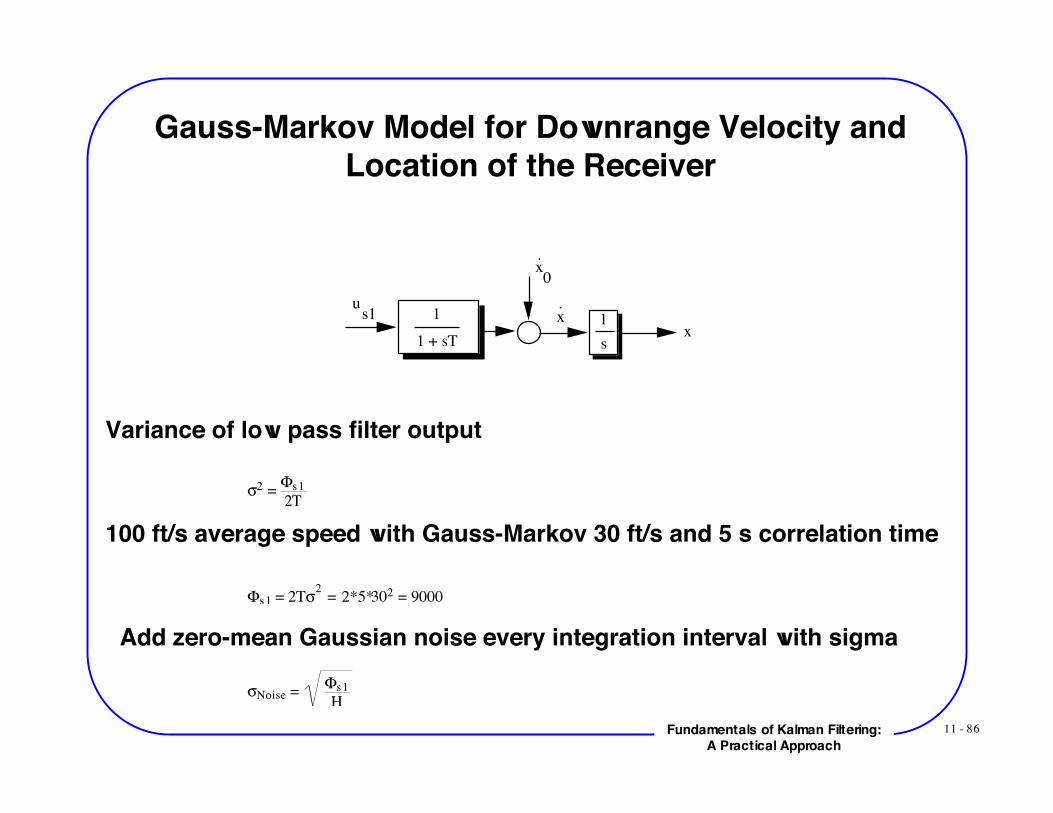
Gauss-Markov Model for Downrange Velocity andLocation of the Receiver
1
1 + sT
1
s
us1
x0
.
x
x.
Variance of low pass filter output
!2 = "s1
2T
100 ft/s average speed with Gauss-Markov 30 ft/s and 5 s correlation time
!s1 = 2T"2 = 2*5*302 = 9000
Add zero-mean Gaussian noise every integration interval with sigma
!Noise = "s1
H
11 - 87Fundamentals of Kalman Filtering:A Practical Approach
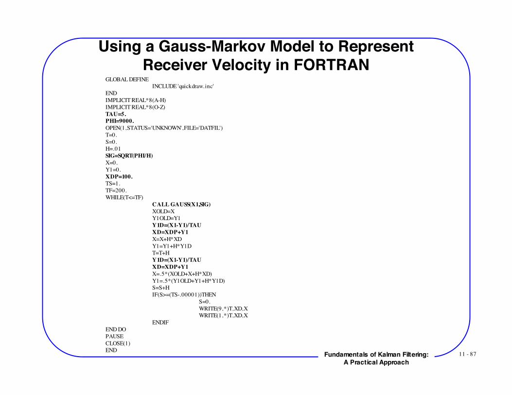
Using a Gauss-Markov Model to RepresentReceiver Velocity in FORTRAN
GLOBAL DEFINE INCLUDE 'quickdraw. inc' END
IMPLICIT REAL*8(A-H)IMPLICIT REAL*8(O-Z)TAU=5.PHI=9000.OPEN(1,STATUS='UNKNOWN',FILE='DATFIL')T=0.S=0.H=.01SIG=SQRT(PHI/H)X=0.Y1=0.XDP=100.TS=1.TF=200.
WHILE(T<=TF) CALL GAUSS(X1,SIG)
XOLD=XY1OLD=Y1Y1D=(X1-Y1)/TAUXD=XDP+Y1X=X+H*XDY1=Y1+H*Y1D
T=T+HY1D=(X1-Y1)/TAUXD=XDP+Y1X=.5*(XOLD+X+H*XD)Y1=.5*(Y1OLD+Y1+H*Y1D)S=S+HIF(S>=(TS-.00001))THEN
S=0.WRITE(9,*)T,XD,XWRITE(1,*)T,XD,X
ENDIFEND DO
PAUSECLOSE(1)END

11 - 88Fundamentals of Kalman Filtering:A Practical Approach
Downrange Velocity of Receiver Varies Quite a Bit
140
120
100
80
60
40
20
0
200150100500
Time (Sec)

11 - 89Fundamentals of Kalman Filtering:A Practical Approach
Downrange Location of the Receiver as a Functionof Time is Nearly a Straight Line
20000
15000
10000
5000
0
200150100500
Time (Sec)
11 - 90Fundamentals of Kalman Filtering:A Practical Approach
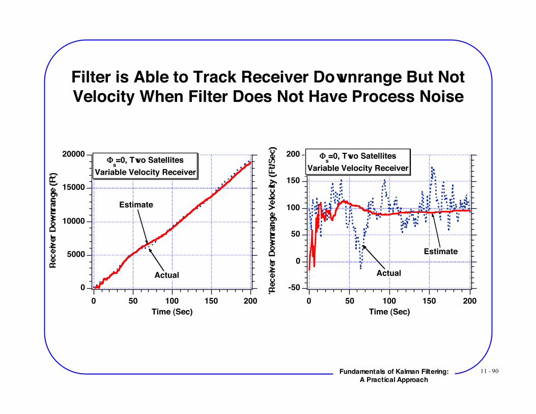
Filter is Able to Track Receiver Downrange But NotVelocity When Filter Does Not Have Process Noise
20000
15000
10000
5000
0
200150100500
Time (Sec)
Actual
Estimate
!s=0, Two Satellites
Variable Velocity Receiver
200
150
100
50
0
-50
200150100500
Time (Sec)
Actual
Estimate
!s=0, Two Satellites
Variable Velocity Receiver
11 - 91Fundamentals of Kalman Filtering:A Practical Approach
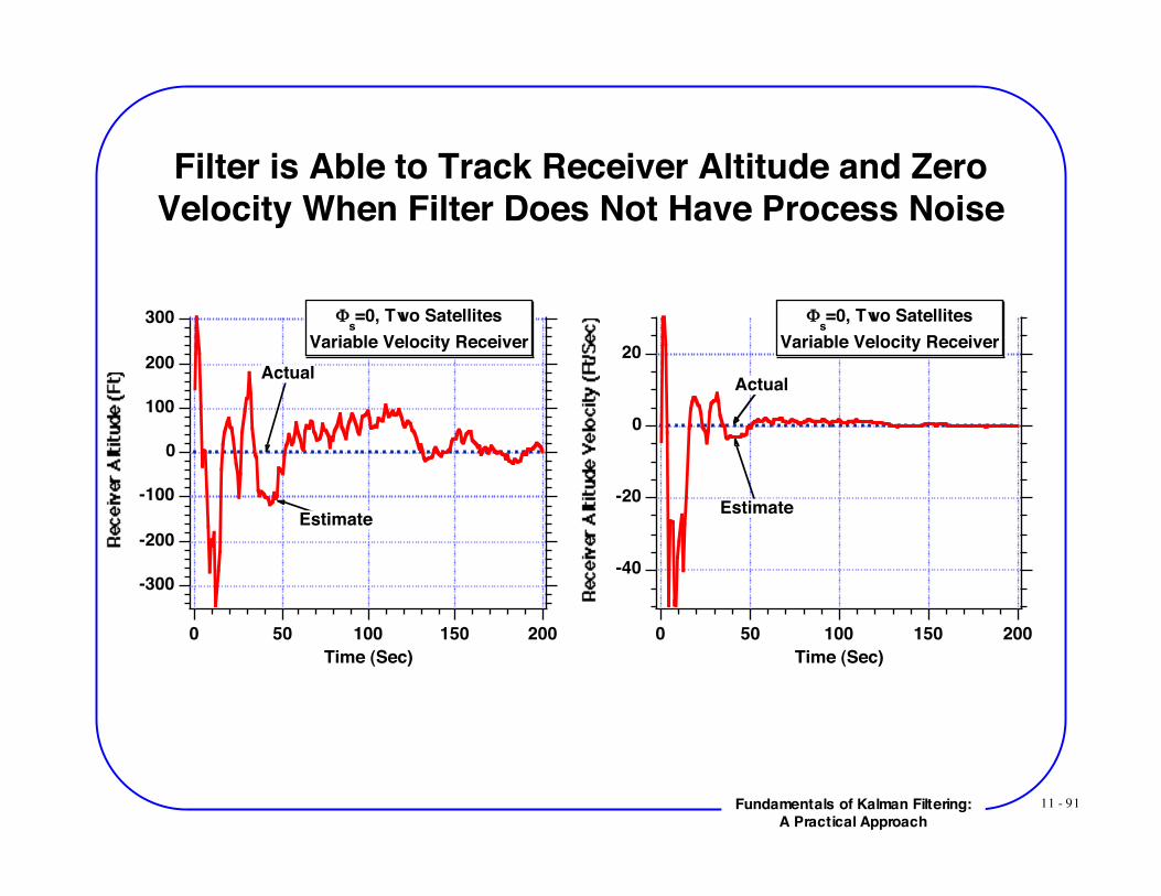
Filter is Able to Track Receiver Altitude and ZeroVelocity When Filter Does Not Have Process Noise
-300
-200
-100
0
100
200
300
200150100500
Time (Sec)
Actual
Estimate
!s=0, Two Satellites
Variable Velocity Receiver
-40
-20
0
20
200150100500
Time (Sec)
Actual
Estimate
!s=0, Two Satellites
Variable Velocity Receiver
11 - 92Fundamentals of Kalman Filtering:A Practical Approach
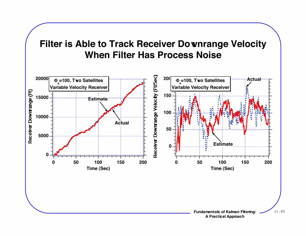
Filter is Able to Track Receiver Downrange VelocityWhen Filter Has Process Noise
20000
15000
10000
5000
0
200150100500
Time (Sec)
!s=100, Two Satellites
Variable Velocity Receiver
Actual
Estimate
200
150
100
50
0
200150100500
Time (Sec)
!s=100, Two Satellites
Variable Velocity Receiver
Actual
Estimate
11 - 93Fundamentals of Kalman Filtering:A Practical Approach
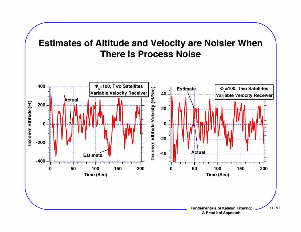
Estimates of Altitude and Velocity are Noisier WhenThere is Process Noise
-400
-200
0
200
400
200150100500
Time (Sec)
!s=100, Two Satellites
Variable Velocity Receiver
Actual
Estimate -40
-20
0
20
40
200150100500
Time (Sec)
!s=100, Two Satellites
Variable Velocity Receiver
Actual
Estimate

11 - 94Fundamentals of Kalman Filtering:A Practical Approach
Error in Estimate of Receiver Downrange andVelocity are Within Theoretical Bounds For Variable
Velocity
-800
-600
-400
-200
0
200
400
600
800
200150100500
Time (Sec)
!s=100, Two Satellites
Variable Velocity ReceiverSimulation
Theory
Theory
150
100
50
0
-50
-100
200150100500
Time (Sec)
!s=100, Two Satellites
Variable Velocity ReceiverSimulation
Theory
Theory
11 - 95Fundamentals of Kalman Filtering:A Practical Approach
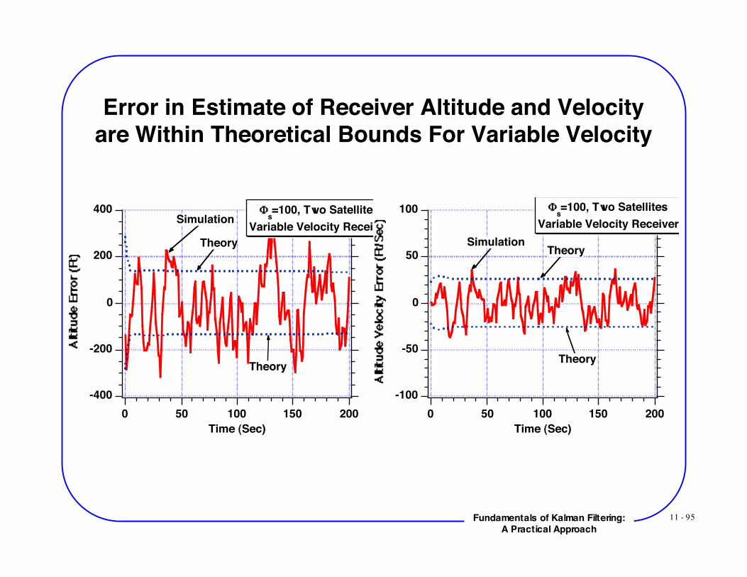
Error in Estimate of Receiver Altitude and Velocityare Within Theoretical Bounds For Variable Velocity
-400
-200
0
200
400
200150100500
Time (Sec)
!s=100, Two Satellites
Variable Velocity ReceiverSimulation
Theory
Theory
-100
-50
0
50
100
200150100500
Time (Sec)
!s=100, Two Satellites
Variable Velocity Receiver
SimulationTheory
Theory
11 - 96Fundamentals of Kalman Filtering:A Practical Approach
Variable Velocity Receiver and Single Satellite
11 - 97Fundamentals of Kalman Filtering:A Practical Approach
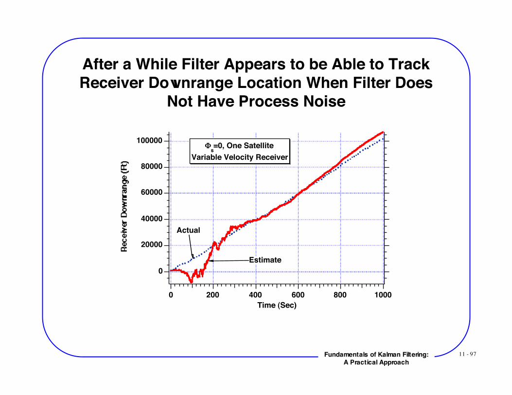
After a While Filter Appears to be Able to TrackReceiver Downrange Location When Filter Does
Not Have Process Noise
100000
80000
60000
40000
20000
0
10008006004002000
Time (Sec)
!s=0, One Satellite
Variable Velocity Receiver
Actual
Estimate
11 - 98Fundamentals of Kalman Filtering:A Practical Approach
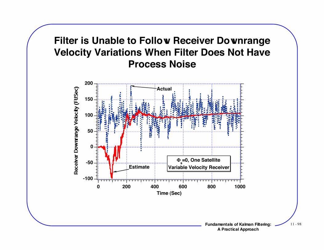
Filter is Unable to Follow Receiver DownrangeVelocity Variations When Filter Does Not Have
Process Noise200
150
100
50
0
-50
-100
10008006004002000
Time (Sec)
!s=0, One Satellite
Variable Velocity Receiver
Actual
Estimate
11 - 99Fundamentals of Kalman Filtering:A Practical Approach
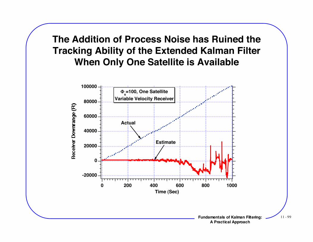
The Addition of Process Noise has Ruined theTracking Ability of the Extended Kalman Filter
When Only One Satellite is Available
100000
80000
60000
40000
20000
0
-20000
10008006004002000
Time (Sec)
!s=100, One Satellite
Variable Velocity Receiver
Actual
Estimate
11 - 100Fundamentals of Kalman Filtering:A Practical Approach
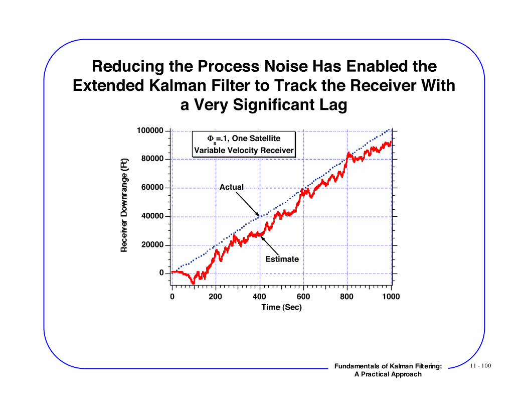
Reducing the Process Noise Has Enabled theExtended Kalman Filter to Track the Receiver With
a Very Significant Lag100000
80000
60000
40000
20000
0
10008006004002000
Time (Sec)
!s=.1, One Satellite
Variable Velocity Receiver
Actual
Estimate
11 - 101Fundamentals of Kalman Filtering:A Practical Approach
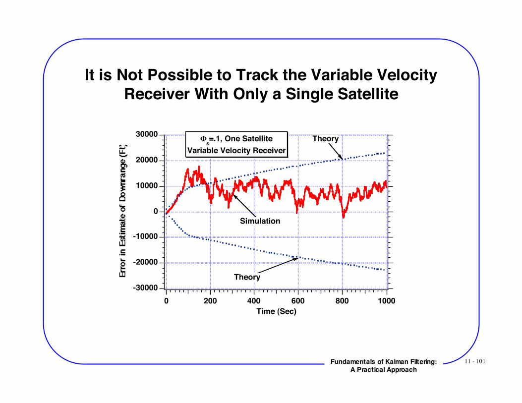
It is Not Possible to Track the Variable VelocityReceiver With Only a Single Satellite
-30000
-20000
-10000
0
10000
20000
30000
10008006004002000
Time (Sec)
!s=.1, One Satellite
Variable Velocity Receiver
Simulation
Theory
Theory
11 - 102Fundamentals of Kalman Filtering:A Practical Approach
Satellite NavigationSummary
• Various options for deriving stationary receiver location basedon noisy range measurements from two satellites
- Linear filtering of range better than no filtering at all- Extended Kalman filter even better
• Satellite geometry is important- Larger angle between range vectors yield better
estimates• Can track stationary receiver with single satellite
- Have problems with variable velocity receiver• Can track variable velocity receiver with two satellites