Embed Size (px)
Citation preview

TUNING AN UNDERWATER
COMMUNICATION LINK
SATISH SHANKAR
NATIONAL UNIVERSITY OF SINGAPORE
2013

TUNING AN UNDERWATER
COMMUNICATION LINK
SATISH SHANKAR
B.E.
A THESIS SUBMITTED FOR THE DEGREE OF
MASTER OF ENGINEERING
DEPARTMENT OF ELECTRICAL & COMPUTER ENGINEERING
NATIONAL UNIVERSITY OF SINGAPORE
2013

DECLARATION
I hereby declare that the thesis is my original work and it has been written by me
in its entirety. I have duly acknowledged all the sources of information which have
been used in the thesis. This thesis has also not been submitted for any degree in
any university previously.
Satish Shankar
26 April 2013
i

ACKNOWLEDGEMENTS
The research described in this thesis was not a solitary e↵ort. Many people
have contributed directly and indirectly, and I am grateful to all of them.
The most significant influence on this thesis is due to my advisor, Prof.
Mandar Chitre. Prof. Mandar’s influence on my life extends even beyond the scope
of this thesis, and has heavily shaped the way i think. His cheerful disposition at
all times, a willingness to always lend a hearing ear, and patient encouragement
over the years have been an incredible gift. For all of these reasons and more, i am
immensely grateful, and extend my heartfelt thanks.
I thank Ahmed Mahmood for the many discussions we had. These discus-
sions helped me in my courses, solidified my understanding, and more importantly,
fuelled my love for signal processing and communications. I also thank my col-
leagues Iulian Topor, Mohan Panayamadam, Rohit Bhatnagar, and Bhavya P.H.
for helping me run experiments and field trials. In particular, Iulian’s e↵orts in de-
bugging modem hardware issues were important in helping me complete the thesis
on time. I also thank the larger Acoustic Research Lab (ARL) community for sup-
porting the research carried out for this thesis and for creating a great environment
to engage in research and development e↵orts.
I thank the many Professors from my undergraduate years for their instruc-
tion. In particular i thank Ms. Micheal Ammal for her support and guidance, which
played an important role in my academic career. I also thank my many friends and
extended family, all of whom have enriched my life and thus contributed indirectly
to this thesis.
Finally i thank my parents and my brother. Their love nourishes and sustains
me. Without them, none of this work would be possible.
ii

Contents
Summary ii
List of Figures iv
Chapter 1 Background 1
1.1 Summary of contributions . . . . . . . . . . . . . . . . . . . . . . . 1
1.2 Thesis organization . . . . . . . . . . . . . . . . . . . . . . . . . . . 1
1.3 Historical overview . . . . . . . . . . . . . . . . . . . . . . . . . . . 2
1.4 Modern underwater communication modems . . . . . . . . . . . . . 3
1.5 Introduction to link tuning . . . . . . . . . . . . . . . . . . . . . . . 5
1.6 Motivation . . . . . . . . . . . . . . . . . . . . . . . . . . . . . . . . 6
1.7 Features of the link tuner . . . . . . . . . . . . . . . . . . . . . . . 7
1.7.1 Data driven link tuning . . . . . . . . . . . . . . . . . . . . 7
1.7.2 Exploration vs exploitation . . . . . . . . . . . . . . . . . . 8
1.7.3 Optimizing for average data rate vs maximum data rate . . 9
1.8 Summary . . . . . . . . . . . . . . . . . . . . . . . . . . . . . . . . 10
Chapter 2 Literature Review 11
2.1 Adaptive modulation . . . . . . . . . . . . . . . . . . . . . . . . . . 11
2.2 Machine learning methods . . . . . . . . . . . . . . . . . . . . . . . 12
2.3 Closely related work . . . . . . . . . . . . . . . . . . . . . . . . . . 13
i

2.4 Summary . . . . . . . . . . . . . . . . . . . . . . . . . . . . . . . . 14
Chapter 3 Problem Formulation and Solution Overview 16
3.1 Problem Formulation . . . . . . . . . . . . . . . . . . . . . . . . . . 16
3.2 Multi armed bandit problem . . . . . . . . . . . . . . . . . . . . . . 18
3.3 Architectural overview . . . . . . . . . . . . . . . . . . . . . . . . . 19
Chapter 4 BER Estimation and Scheme Generation 22
4.1 Kalman filter for bandit arm . . . . . . . . . . . . . . . . . . . . . . 23
4.1.1 Model . . . . . . . . . . . . . . . . . . . . . . . . . . . . . . 24
4.1.2 Filter update equations . . . . . . . . . . . . . . . . . . . . . 26
4.2 FEC selection logic . . . . . . . . . . . . . . . . . . . . . . . . . . . 26
4.3 Scheme generator . . . . . . . . . . . . . . . . . . . . . . . . . . . . 28
Chapter 5 Bandit Selection Algorithms 33
5.1 Dynamic programming solution . . . . . . . . . . . . . . . . . . . . 33
5.1.1 Link tuning as sequential decision optimization . . . . . . . 33
5.1.2 Dynamic programming equations . . . . . . . . . . . . . . . 35
5.2 Softmax Exploration . . . . . . . . . . . . . . . . . . . . . . . . . . 36
5.3 ✏-greedy . . . . . . . . . . . . . . . . . . . . . . . . . . . . . . . . . 36
5.4 Pursuit algorithm . . . . . . . . . . . . . . . . . . . . . . . . . . . . 37
5.5 Upper Confidence Bounds (UCB) . . . . . . . . . . . . . . . . . . . 37
5.5.1 UCB1 . . . . . . . . . . . . . . . . . . . . . . . . . . . . . . 37
5.5.2 UCB1-Tuned . . . . . . . . . . . . . . . . . . . . . . . . . . 38
Chapter 6 Results 39
6.1 Test setup . . . . . . . . . . . . . . . . . . . . . . . . . . . . . . . . 39
6.2 Simulation results . . . . . . . . . . . . . . . . . . . . . . . . . . . . 40
6.3 Watertank tests . . . . . . . . . . . . . . . . . . . . . . . . . . . . . 42
ii

6.4 Test at RSYC . . . . . . . . . . . . . . . . . . . . . . . . . . . . . . 43
6.5 Summary of results . . . . . . . . . . . . . . . . . . . . . . . . . . . 46
Chapter 7 Analysis and Interpretation of Results 48
7.1 Evolution and clustering of schemes . . . . . . . . . . . . . . . . . . 53
7.2 Visualizing RSYC trial data . . . . . . . . . . . . . . . . . . . . . . 59
7.3 Summary . . . . . . . . . . . . . . . . . . . . . . . . . . . . . . . . 64
Chapter 8 Conclusion 66
8.1 Summary of contributions . . . . . . . . . . . . . . . . . . . . . . . 66
8.2 Conclusion . . . . . . . . . . . . . . . . . . . . . . . . . . . . . . . . 66
8.3 Further research . . . . . . . . . . . . . . . . . . . . . . . . . . . . . 67
Appendices vi
Chapter A Related Publications 1
iii

Summary
The characteristics of an underwater communication channel vary widely, de-
pending on depth, temperature gradients, ambient noise levels, etc. The data rate
performance of an underwater modem also varies with the nature of the channel.
Advancements in computer architecture have lead to the development of underwa-
ter communication modems that implement a diverse array of communication and
signal processing algorithms in software. Software based implementations of com-
munication algorithms give us an opportunity to continuously tune their parameters
at runtime.
This thesis develops a family of algorithms that can continuously tune the
parameters of any modem implementation, aiming to optimize the data rate per-
formance in any given channel. These algorithms tune the parameters for a point-
to-point underwater communication link and aim to maximize the average data
rate. Since a link tuner that can work with any modem implementation is sought,
a data driven approach to tuning is pursued, instead of a physics driven approach.
Hence the link tuner only requires bit error rate information in order to make tuning
decisions.
The exploration vs exploitation dilemma arises as a recurrent theme in this
thesis. At every transmission opportunity, the link tuner can explore new parameter
values in order to make better future decisions. Alternatively, the tuner could
exploit existing knowledge and improve the data rate performance now. Pursuing
a purely exploration or exploitation based strategy leads to poor performance, and
finding a balance is key to achieving high data rates.
The tuner aims to maximize the average data rate, rather than attain the
maximum possible data rate. The time taken to tune the link is included in our
iv

computation of average data rate. This distinction highlights the need to develop
online mechanisms for link tuning, in contrast to running an o✏ine search for the
best performing scheme and storing it. The need for online tuning also evident
by considering the variety of underwater channels: as the channel characteristics
change, modem parameters need to update in order to consistently maintain data
rate performance.
The algorithms developed in the thesis are implemented on the UNET-II
modem. The UNET-II modem is developed by the Acoustic Research Lab (ARL),
and is based on orthogonal frequency division multiplexing. Results from simula-
tion, tank tests and field trials at the Republic of Singapore Yatch Club (RSYC)
demonstrate a significant improvement in average data rate as compared to the
average data rate attained without tuning. Experimental results are augmented
with analysis and visualizations that provide insight into the mechanisms of link
tuning.
v

List of Figures
3.1 Link tuner architecture . . . . . . . . . . . . . . . . . . . . . . . . 20
4.1 Kalman filter for BER estimation . . . . . . . . . . . . . . . . . . . 23
4.2 Nonlinear mapping from BER to state . . . . . . . . . . . . . . . . 25
4.3 Code rate vs BER . . . . . . . . . . . . . . . . . . . . . . . . . . . 27
4.4 Evolution of probability density curves used by scheme generator . 31
6.1 Average data rate in simulation . . . . . . . . . . . . . . . . . . . . 40
6.2 Instantaneous data rate observed in simulation . . . . . . . . . . . 41
6.3 Average data rate in tank . . . . . . . . . . . . . . . . . . . . . . . 43
6.4 Average data rate in tank at end of test . . . . . . . . . . . . . . . 44
6.5 RSYC test site . . . . . . . . . . . . . . . . . . . . . . . . . . . . . 44
6.6 Average data rate at RSYC . . . . . . . . . . . . . . . . . . . . . . 45
6.7 Average data rate at RSYC at end of test . . . . . . . . . . . . . . 46
6.8 Instantaneous data rates observed at RSYC . . . . . . . . . . . . . 47
7.1 Evolution of number of carriers sampling and selection (simulation) 49
7.2 Evolution of prefix length sampling and selection (simulation) . . . 49
7.3 Link tuning represented as a graph (water tank data, DP algorithm) 51
7.4 Node ID versus the number of times the node was tried (+1) . . . 52
7.5 Ego network centered at node 52 . . . . . . . . . . . . . . . . . . . 54
vi

7.6 Ego network centered at node 20 . . . . . . . . . . . . . . . . . . . 55
7.7 Ego network centered at node 9 . . . . . . . . . . . . . . . . . . . . 56
7.8 Evolution of the graph in Fig. 7.3 . . . . . . . . . . . . . . . . . . . 58
7.9 Graph representation of link tuning data (RSYC data, DP algo-
rithm) . . . . . . . . . . . . . . . . . . . . . . . . . . . . . . . . . . 60
7.10 Legend for Figure 7.9: node color, scheme type and percentage oc-
currence of node in graph . . . . . . . . . . . . . . . . . . . . . . . 62
7.11 Evolution of number of carriers sampling and selection (RSYC data) 63
7.12 Evolution of prefix length sampling and selection (RSYC data) . . 63
vii

1. Background
1.1 Summary of contributions
1. A family of learning algorithms to tune an underwater communication link
are derived.
2. A data driven approach to link tuning is pursued, leading to the development
of a tuner that works with any modem implementation, and requires only bit
error rate information as input.
3. Results from performance tests in: a) simulation, b) water tank, and c) field
trials demonstrate a significant improvement in average data rates.
4. An extensive analysis and discussion of results is presented in order to provide
insight into the mechanism of link tuning.
1.2 Thesis organization
Chapter 1 begins with a brief historical overview of underwater acoustic commu-
nications followed by an introduction to and the motivation for the link tuning
problem. The key design features of the link tuner are described. The ideas in
this thesis lie in the intersection of the fields of adaptive modulation and machine
learning. The relevant literature from these fields is reviewed in chapter 2. Chapter
1

3 presents a mathematical formulation for the link tuning problem followed by an
architectural overview of the solution. Chapters 4 and 5 describe bit error rate es-
timation, scheme generation and bandit selection algorithms used in the link tuner.
Chapter 6 documents results from performance tests conducted in a) simulation,
b) water tank, and c) field trials. Chapter 7 contains discussions and visualizations
to provide insight into the mechanism of link tuning. Finally we finish with a brief
discussion of further research directions that may lead to the next generation of
link tuners.
1.3 Historical overview
Underwater acoustic communication (UAC) is a key enabling technology for a vari-
ety of applications, such as autonomous underwater vehicles, collection of scientific
data recorded by sensors on the ocean floor, pollution and environment monitoring
systems, and diver communication equipment. UAC development can be traced
back to submarine telephones developed by the Unites States Navy in the second
world war period. These devices used single side-band suppressed carrier modula-
tion signals in the 8-11 KHz range and were capable of sending acoustic signals over
several kilometers. With much more powerful computing systems today, it’s now
possible to implement complex signal processing and communication algorithms on
a modem that runs on a modest amount of power.
There are many papers that provide a comprehensive review of UAC, includ-
ing [1] and [2]. Modern acoustic signal processing has advanced the state-of-the-art
for communication technology significantly. Some examples of these advancement
include: 1) acoustically controlled robots for maintenance tasks of submerged plat-
forms [3], 2) video transmission from a 6500 meter deep ocean trench [4], and 3)
data telemetry in excess of 200 kilometers [5].
Of course, acoustics is not the only choice for wireless communication in
2

an underwater channel. However, radio waves with frequencies beyond 300 Hz
attenuate too rapidly for practical use, thus necessitating the use of large antennae
and high powered transmitters. The other option lies in transmission of optical
signals by using lasers. Optical signals do not su↵er as much from attenuation.
However, they are highly sensitive to scattering e↵ects. This requires one to use
highly directed laser beams and yet achieve a range of the order of only a few
meters.
Advancements in VLSI technology and computer architecture have resulted
in modems that are increasingly software driven. Software driven modems allow
us to implement a wider variety of algorithms, and the possibility of tuning the
parameters of those algorithms emerges. In this thesis, we are interested in devel-
oping a general method of improving the data rate performance of a communication
modem with tunable parameters.
1.4 Modern underwater communication modems
Teledyne Benthos, LinkQuest and Evologics are the major commercial providers of
underwater modems. There are also underwater modems developed by university
labs such as the WHOI micro modem [6], the UCSD modem [3] and the UNET-II
modem [7]. Teledyne Benthos and LinkQuest modems o↵er data rates of 2.4 and 9.6
kbps [3]. The WHOI micro modem o↵ers data rates of 0.08 to 5.4 kbps depending
on the modulation scheme selected, whereas the UCSD modem has a data rate of
200 bps [3].
In reality, depending on the channel, the measured data rates may di↵er sig-
nificantly from the ones cited above. For example, the Evologics modem [8] (S2C
modem) claims to work at upto 33 kbps [9]. These data rates were tested in the
Baltic sea. However, in a 2004 experiment conducted in Singapore waters, the Evo-
logics modems were only able to transmit at about 6 kbps at 10 m range, steadily
3

reducing to about 1 kbps at 90 m range, and failing to achieve a consistent link
beyond the 100 m range [9]. Note that the Evologics modems have been success-
fully tested at longer ranges since that experiment. Nevertheless, this serves as an
illustrative example of the e↵ects of di↵erent channels on the data rate performance
of the same modem implementation.
Underwater communication modems also feature a diverse variety of physical
layer implementations. For example, the Evologics modem is based on a sweep
spread spectrum communication scheme. The WHOI micro modem is based on a
frequency-shift keying with frequency hopping scheme, while the UNET-II modem
is based on orthogonal frequency division multiplexing (OFDM). Depending on the
implementation, each of these modems have some parameters that can be tuned.
As the processing power on chips continues to increase, we are likely to see even
more diversity in the physical layer implementations for underwater modems of the
future.
According to the Shannon capacity theorem, data rate is limited by the avail-
able bandwidth and power. There exist practical limitations imposed on bandwidth
by the attenuation characteristics of the underwater channel, ambient noise condi-
tions, transducer characteristics, and so on. Similarly, power is limited by trans-
ducer characteristics and cavitation processes [10], among other things. Increasing
power also increases inter symbol interference and may not always lead to improved
data rate performance. Underwater acoustic channels are both bandwidth as well
as power limited. Various other physical phenomena impose other limiations on the
underwater channel. Di↵erent physical layer implementations together with widely
varying channel conditions point to the need for a general link tuning algorithm
that can adapt the parameters of any particular physical layer implementation in
response to channel conditions.
We test our link tuning algorithms on the UNET-II modem. This modem is
4

based on OFDM. The default settings on the modem o↵ers a data rate of 345 bps.
Under the right channel conditions, the data rate can increase to a maximum of
about 11 kbps. These numbers serve as context to the reader in terms of the range
of data rates that we can experience on our modem of choice for the implementation
of the ideas proposed in this thesis.
1.5 Introduction to link tuning
We seek to improve the performance of underwater communication systems by de-
veloping algorithms that can tune a point-to-point underwater communication link.
The design and implementation of an underwater communication system includes
a number of subsystems, including algorithms for modulation and error correction
coding. As our hardware capabilities increase, it is possible to implement ever more
rich and varied kinds of communication algorithms to maximize the performance of
a modem. In particular, many algorithms are implemented in software. This opens
up the possibility of modifying the parameters of a modem at runtime in response
to the channel conditions.
For any given modem implementation, the data rate performance of a link
depends on the parameters of the communication algorithms in use. Determining
what might be a good set of parameter values to use in a given channel is critical
for achieving high data rates. The capability of having software control on these
parameter values means that one does not need to decide in advance what values
to set these parameters to. Instead, we can continuously tune them, in response to
the channel conditions. This thesis describes the algorithms and implementation of
such a link tuner. In particular, we implement link tuning algorithms to maximize
the average data rate in an underwater communication link. We implement our
link tuner in the UNET-II modem and present field trial results.
5

1.6 Motivation
The motivation for a link tuner arises from:
1. The large number of possible configurations for a link.
2. The need for an online tuning mechanism.
For modems with a variety of configurable parameters, the space of parameter values
can quickly grow to be large. As an illustrative example, consider the UNET-
II modem developed at the Acoustic Research Lab (ARL) [7]. The modulation
system is based on OFDM. It is possible to set values for the following parameters:
1. Modulation mode (coherent / incoherent or QPSK / BPSK).
2. Di↵erential mode (time or frequency).
3. Prefix / su�x length (values range from 0 to 1024)
4. Number of carriers (64,128,256,512,1024)
5. Number of nulls (values range from 0 to 1024)
6. Error correction type (Convolution, Golay, both or none)
Together, they represent 10’s of millions of possible configurations.
The need for an online tuning mechanism is evident by considering the dy-
namic nature of the underwater channel. There is no such thing as a “typical”
underwater channel [11]. The channel response changes with location, water depth,
temperature/salinity profiles, modulation methods used, frequency of operation,
tidal cycles, and a myriad of other factors. That makes it impossible to search for
the best set of parameter values o✏ine and store them. Hence we need a mechanism
for online tuning, so that we can continuously make improvements to the average
data rate in response to any channel.
6

1.7 Features of the link tuner
The link tuner that we develop has three characteristic feautures. Firstly, we use
a data driven approach to link tuning, as opposed to a physics driven approach.
Secondly, the exploration versus exploitation dilemma plays a key role in the design
of the link tuner. Finally, the tuner aims to optimize for the average data rate,
rather than attain the maximum possible data rate.
1.7.1 Data driven link tuning
We adopt a data driven approach to link tuning. Specifically, we make a series of
choices for parameter values based only on bit error rate data.
An alternative approach to developing such a link tuner would be to base
it on our knowledge of the channel from a physics based model. Such a model
would need to describe the interaction between a given underwater channel and the
communication signals generated from our modem.
However, rather than study physics based models, we instead choose to use
a data driven approach to drive our link tuner. Doing so has two advantages: a)
simplicity in terms of input requirements to the tuner, and b) decoupling of the
tuner from the modem implementation.
The input to our data driven link tuner simply consists of bit error rate
data. In contrast, physics based models are based on information such as ab-
sorption/spreading loss [11], ray/beam tracing information [12], Doppler / delay
spread [13], and so on. Bit error rate information is a fundamental quantity in
a communication system, so one may safely assume its availability. On the other
hand, spreading losses, etc. are harder to obtain, often requiring the modem to
process custom signals and expose special interfaces.
A data driven tuner has another advantage over a physics driven tuner: it
7

is not coupled to any particular modem implementation. A single data driven link
tuning framework can operate on di↵erent modems and it remains useful even as
the underlying physical layer implementation evolves and changes.
Relying only on bit error rate information and independence from the un-
derlying physical layer implementation prove to be critical advantages that cement
our decision to use a data driven approach to linktuning.
1.7.2 Exploration vs exploitation
One can think of the link tuner as a learning agent that tries to learn a mapping
from a given state to an action in order to maximize a numerical reward signal
returned by the environment. In our case, the state consists of our knowledge, the
action space corresponds to the set of available parameter configurations, and the
reward corresponds to the data rate.
In order to make better choices in the future, the agent needs to try new
actions by exploring the action space. But in order to generate more reward, the
agent needs to exploit its existing knowledge. This leads us to a central theme:
that of balancing exploration versus exploitation. Pursuing a purely exploration or
exploitation based policy leads to poor performance, so we need to find some sweet
spot in the middle. Balancing exploration and exploitation is critical for achieving
high average data rates.
In a supervised learning situation, which is more commonly discussed in
machine learning literature, an agent is supplied with sample vectors and output
results from an external oracle. In our scenario, we have no examples of how a
particular configuration might perform at the outset. Instead, the tuner needs to
learn this mapping by interacting with the channel.
8

1.7.3 Optimizing for average data rate vs maximum data
rate
We are concerned with the whole problem of maximizing the average data rate,
rather than attaining the maximum possible data rate. We measure the average
over the course of a data transfer. The time taken to tune the link is included while
measuring the average data rate. It may be possible to devise a search algorithm
to search for the configuration with the maximum possible data rate. We can run
the search process until either we have examined all configurations, or we meet a
stopping criterion such as a timeout or we have discovered a configuration with
data rates higher than a pre-set threshold. Rather than decide on an arbitrary
stopping criterion, we aim to maximize the average data rate. In other words, we
aim to optimize the entire sequence of parameter configurations that are tried out
in the process of link tuning.
Average data rate computation includes the time consumed by the tuning
process. From a user’s point of view, this is a better metric to optimize for as
compared to maximum data rate. The motivation of optimizing for average data
rate can be better understood by considering the role of the link tuner in a data
transfer situation. Attaining the maximum data rate would entail sampling a suf-
ficient number of schemes to infer the scheme that has the maximum possible data
rate. If the search space is large, and only a tiny amount of data needs to be
transferred, the tuner will spend a disproportionate amount of time in the search
process (as compared to the data transfer time) if we optimize for maximum data
rate. The link tuner client will have to wait until the search process terminates
before any data transfer can be initiated. It is also possible that the channel may
change fast enough that the search process never terminates because older results
become obsolete too soon. On the other hand, optimizing for average data rate
9

accounts for the time spent in the search process. This ensures that a link tuner
client continously experiences better data rates over time, regardless of the amount
of data to be transferred.
1.8 Summary
Software implementations of communication modems allow us to modify modem
parameters at runtime. The increasing variety and sophistication of modem im-
plementations, widely varying characteristics of underwater channels, and a large
search space for modem parameter values motivate the need for a link tuner that
is capable of optimizing the parameters of any modem implementation. We seek
a link tuner that continously modifies modem parameters in an online mode in
response to varying channel characteristics. The advantages of using a data driven
approach to tuning, rather than a physics driven approach is explained. The explo-
ration vs exploitation dilemma, which plays a central role in the development of the
link tuner, is described. The link tuner aims to optimize for the average data rate,
rather than attain the maximum possible data rate. This important distinction
is reviewed. We implement the ideas proposed in this on the UNET-II modem.
The default settings on this modem yield a data rate of 345 bps. Under the right
channel conditions, the data rate can increase to a maximum of about 11 kbps. We
list the various tunable parameters on this modem and point out the large number
of total possible configurations. The need for an online mechanism for link tuning
is explained. These numbers provide the reader with context in terms of the range
of data rates that we can experience in the tuning process.
10

2. Literature Review
Literature related to the ideas in this thesis are found in the fields of adaptive mod-
ulation, especially for terrestrial wireless/cognitive radios, as well as machine learn-
ing. We first cite literature to provide a general overview of these fields. Though
none of them directly apply reinforcement learning [14] algorithms to develop an
underwater link tuner, we review some work that has close parallels to the ideas
explored in this thesis. Finally we explain the critical di↵erences between closely
related work and how we build on it.
2.1 Adaptive modulation
Parallels to our work can be found in adaptive modulation techniques developed for
terrestrial wireless radio networks and in the cognitive radio domain. For a sampling
of literature from these areas, see [15], [16] and [17]. Many of these techniques focus
on optimizing energy / spectral e�ciency. The adaptation schemes often make use
of SNR information and in the case of MIMO-OFDM systems, of spatial diversity
/ beamforming. See [17] for an example of application of such techniques to 802.11.
There has also been considerable research e↵ort directed towards channel
estimation algorithms in both terrestrial wireless networks as well as the underwater
communication domain. See [18], [19] and [20] for a sampling of channel estimation
literature. We draw attention to [21] as a piece of work which contains similar
11

ideas as the ones proposed in this thesis. The authors develop a stochastic learning
automaton for adapting an ODFM link. The adaptation is based on estimating bit
error rates for various modulation and coding schemes and comparing them with
associated threshold bit error rate levels.
2.2 Machine learning methods
A distinctive feature of this thesis is the application of machine learning methods
to digital communication. In 1959, Arthur Samuel defined machine learning as a
“Field of study that gives computers the ability to learn without being explicitly
programmed”. See [22] for a comprehensive overview of this field. The space of
machine learning algorithms can be divided into 3 primary partitions: a) super-
vised learning, b) unsupervised learning and c) reinforcement learning. Supervised
learning is concerned with the inference of a function from labeled training data.
The training data consists of a set of objects, which are usually vectors derived from
the features of the underlying phenomena of interest. The labels may be discrete
or continuous valued, and the corresponding inferred functions are called classifiers
or regressors. Unsupervised learning methods seek to find existing structure in un-
labeled data. In contrast to supervised learning, unsupervised learning methods do
not require labels. The absence of an error or reward signal to evaluate a poten-
tial solution characterizes unsupervised learning. K-means clustering and principal
component analysis are examples of unsupervised learning.
Reinforcement learning is concerned with a learning by interaction [14].
Specifically, an agent seeks to take actions in an environment to maximize its
cumulative reward. In contrast to supervised learning, the agent is not presented
a set of training examples with labels.Instead, the agent needs to generate its own
set of training data by interacting with the environment. The focus in this setting
lies in the agent’s online performance. There is a critical need to balance between
12

an exploration of uncharted space and the exploitation of existing knowledge.
The learning algorithms explored in this thesis are categorized under rein-
forcement learning. [14] provides a comprehensive review of reinforcement learning
algorithms. We use the multi armed bandit problem [23] as our model of choice
for studying the tradeo↵ between exploration and exploitation. The multi armed
bandit problem has been well studied and there exists a rich body of literature
containing many algorithms to solve the problem and its variants. We specially
draw attention to the Gittins index [24] because it gives an optimal policy for max-
imizing the expected discounted reward. The Gittins index has also been heavily
used in some of the closely related work to this thesis [25], [26] and [27].We also
point to the upper confidence bounds (UCB) family of algorithms [28] because they
are regarded as the state of the art algorithms in a classical multi armed bandit
setting [29]. We implement and compare UCB algorithms in this thesis.
2.3 Closely related work
The most closely related work in terms of applying reinforcement learning methods
to a communication link is done by Haris et. al. in [25], [26] and [27]. The authors
try many exploration heuristics such as Boltzmann, ✏-greedy and Gittins index-
ing [24] methods (among others) to optimize the bit rate per hertz of a cognitive
radio. We also point out [30] and [31], which are the only literature we know of that
discuss reinforcement learning ideas applied to an underwater communication link.
The authors try exploration heuristics similar to Boltzmann and ✏-greedy methods,
and also develop other custom strategies.
This thesis builds on the above literature. A distinctive feature of this thesis
is that we address 3 aspects of the tuning problem which are not considered above.
These aspects turned out to be critical to achieving a high performance link tuner.
We elaborate on these aspects of the tuning problem below:
13

1. Finite vs. infinite search space: The above literature implicitly assumes that
the search space for a tuner is finite. In practice, the set of candidate search
points under consideration by the tuner would need to be reasonably small in
order to meet memory and time limitations for implementation on a practical
system. We present here a technique for dynamically generating new candi-
date search points in response to past results. This allows us to consider a
very large search space, enabling us to run fine-grained tuning process.
2. Estimation of packet success rates: We use a Kalman-filtering approach to
fuse information from user data packets along with training packets to get
bit error rate estimates. We then extrapolate this knowledge to obtain final
reward estimates. This approach better utilizes the incoming stream of packet
information, compared to simply counting the number of successful / failed
packet transmissions and estimating a packet success rate from that.
3. Arbitrary reward distribution: Some of the more sophisticated techniques
examined in the above works (such as the Gittins index [24]) require that all
actions yield the same reward upon success. As an alternative to the Gittins
index, we derive a dynamic programming based index that does not require
all actions to yield equal reward.
2.4 Summary
The ideas proposed in this thesis are drawn from an intersection of the fields of
adaptive modulation and machine learning. We reviewed literature that provides
a broad overview of these fields. With respect to adaptive modulation, one can
find similar techniques developed for wireless radio networks as well as cognitive
radio. Machine learning can be broadly divided to supervised, unsupervised and
reinforcement learning methods. The algorithms used in this thesis are classified
14

under the umbrella of reinforcement learning. Finally, we reviewed a small, but
specific set of papers that are closely related to our work in terms of applying
reinforcement learning methods to a communication link. We explain the critical
di↵erences between the closely related work and how this thesis builds on top of
those ideas.
15

3. Problem Formulation and
Solution Overview
A mathematical formulation of the link tuning problem is described. We describe a
high level overview of the architecture of the proposed link tuning solution. The link
tuner consists of 3 components: a BER estimator, a scheme generator, and scheme
selection algorithms. The inputs to the tuner consist of a set of measurements.
The tuner outputs scheme recommendations. The multi armed bandit problem is
a key concept used in the design of the link tuner. It is necessary to understand
the multi armed bandit problem before we describe the link tuner architecture in
further detail.
3.1 Problem Formulation
We define a scheme s 2 S to be a vector that contains the values of each parameter
we wish to tune. s
pi
denotes a packet encoded in scheme i. We can apply an
encoding c 2 C to a packet, yielding an information rate of 0 r
c
1. The
information rate is defined as the the ratio of the user data carrying bits to the
total bits in the packet. The information rate accounts for all header bits. We have
2 types of packets, depending on the encoding c applied to them: data packets and
test packets.
16

The encoding applied to a data packet is an error correction code. Since
error correction coding is also popularly known as forward error correction (FEC)
in literature, we shall henceforth use both terms interchangeably. A data packet
has an information rate r
c
that is equal to the code rate of the FEC it is encoded
with.1
Test packets do not use any error correction coding. Test packets are pre-
generated bit patterns, useful for BER estimation. A test packet has an information
rate of zero. A modem can recieve a test packet n bits in length and can compute
the number of bits k that were erroneously received.
Based on the above descriptions of data and test packets, we note that the
general notions of an encoding c with information rate r
c
applies to all packets.
However in the context of data packets, these correspond to an error coding scheme
c with a code rate r
c
.
We define the uncoded data rate of a scheme �
j
to be equal to the data
rate that one would obtain by setting r
c
= 1. �
j
corresponds to an under-specified
scheme (it does not specify the encoding c). For a data packet, it is equal to the
data rate that would result by not employing any FEC.
For a given �
j
, we arrive at scheme i (a complete specification) if we also
specify the information rate r
c
. Note the correspondence between i ⌘ (j, c). A
packet s
pi
encoded in scheme i is equivalently encoded in s
pj,c
. Upon successful
reception, s
pi
yields an instantaneous data rate of �
j
r
c
.
Each error coding scheme c can tolerate an uncoded bit error rate upto a
certain threshold T
c
. We compute the value of T
c
depending on the FEC used.
For example, a [24, 12, 8] Golay code is a block code that carries 12 bits of user
information in a 24 bit code word. It is capable of correcting upto 3 error bits. If
1Information rate is a general concept that follows from the notion of applying an encoding topackets, and is applicable to both test as well as data packets. In the case of data packets, thisencoding is an error correction code, and the code rate is equal to the information rate.
17

we assume that bit errors are independently distributed, a bit stream encoded with
this FEC will not tolerate an average bit error rate greater than 3/24 = 12.5%. In
general the lower the code rate, greater the threshold tolerance T
c
.
We have a point-to-point communication link that can return feedback on
our scheme choices. For test packets, the receiver reports the number of erroneous
bits k. For a data packet, the receiver reports successful / failed reception. We
are free to switch to any scheme at every transmission opportuinity.The modems
use a control scheme for communicating control information such as as number of
erroneous bits or packet reception success / failure. The control scheme is a robust,
low data rate scheme. It does not get tuned and is used only for communicating
control information.
Given the above setup, we seek to compute a sequence of schemes to maxi-
mize the average data rate.
3.2 Multi armed bandit problem
We use the multi armed bandit (MAB) problem as a model for the link tuning
process [23]. Suppose one is presented with a set of slot machines. When played, a
machine yields some reward as per an unknown probability distribution. The multi
armed bandit problem is defined as follows: in what sequence must one play the
machines to maximize the total expected reward? The MAB problem represents
the exploration versus exploitation dilemma inherent in situations like link tuning
where an agent needs to learn by interacting with the environment. When a slot
machine (also referred to as a bandit arm) is played, we gain knowledge about its
probability distribution. At any point, we are faced with a choice. We could either
gain more knowledge by playing new bandit arms, or we could exploit our existing
knowledge to maximize the current reward. Balancing this tradeo↵ holds the key
to attaining a good performance.
18

The mapping between the MAB problem and the link tuning process is as
follows: a bandit arm in the MAB problem is defined to be the same as a scheme,
except that the encoding c is left unspecified. A bandit arm j together with an
encoding c defines a scheme i. Thus each bandit arm can be associated with multiple
schemes, depending on the choice of c. A packet s
pi
corresponds to scheme i, bandit
arm j, and an encoding of information rate r
c
. Note the correspondece between
the indices i ⌘ (j, c) as described in chapter 3. The uncoded data rate of s
pi
is �
j
.
If s
pi
is successfully received, it yields an instantaneous data rate of �
j
r
c
.
3.3 Architectural overview
Fig. 3.1 shows a high level overview of the link tuner architecture. The input
to the link tuner consist of measurements. The output of the link tuner consists
of recommendations for which scheme to use for the next tranmission. The link
tuner itself consists of 4 components: a database of schemes, a scheme generator,
a BER estimator, and a scheme selector. The link tuner is used in the context of a
point-to-point communication link with BER feedback. The transmitter decides to
switch to a particular scheme, and transmit packets encoded in that scheme. The
receiver reports success/failure if data packets were received, and k if a test packet
was received. The link tuner is fed these two pieces of information, from which we
derive the measurements referred to in Fig. 3.1.
The BER estimator consists of a set of Kalman filters. We maintain a
Kalman filter for each bandit arm. The relationship between the BER estimates
for a scheme and a bandit arm is explained in section 4.2. These filters estimate
the BER for their corresponding arm. This information is used to compute the
expected data rate for that scheme, which in turn is used by the scheme selector.
The scheme selector is responsible for selecting a scheme from the scheme database.
The selection logic is governed by bandit algorithms, which we explore several of.
19

Figure 3.1: Link tuner architecture
20

These algorithms work by either computing an index value for each scheme and
selecting the scheme with the highest index value, or by maintaining an explicit
policy over the arms, whose updates are informed by empirical means. Note that
the term index in the previous sentence refers to a value that is computed for a
scheme based on its history of rewards. The scheme generator adds new schemes to
the database at periodic intervals. Since the parameter space is exceedingly large,
it is impractical to enumerate all schemes and maintain indices/policies over all of
them. The scheme generator overcomes this problem by progressively adding new
schemes to the scheme database. The principle for generating new schemes is that
we sample points in the region surrounding the better performing schemes as time
progresses. The generation policy is based on heuristics that are informed by our
experience.
21
4. BER Estimation and Scheme
Generation
The BER estimator aims to maintain a BER estimate for each bandit arm. It is
implemented as a set of Kalman filters, such that each bandit arm has an associ-
ated Kalman filter. The inputs to the Kalman filter consist of either data packet
measurements or test packet measurements. We define the system model for the
Kalman filter in terms of measurement functions, and we derive the filter update
equations for time / measurement updates. The BER estimates determine the
choice of FEC used. We describe the FEC selection logic and explain the relation-
ships between BER estimates, code rate thresholds, packet success probability and
data rate estimates.
The scheme generator adds new schemes to the scheme database at periodic
intervals. Since the parameter space is large, it is impractical to enumerate all
schemes and maintain policies over them. The scheme generator overcomes this
problem by progressively adding new schemes to the database. The scheme gener-
ation logic is driven by the results of previous transmissions. The main principle
governing the scheme generator is that of progressively sampling the region sur-
rounding the better performing schemes. We describe the heuristics used by the
scheme generator and the rationale governing our choice of heuristics.
22

Figure 4.1: Kalman filter for BER estimation
4.1 Kalman filter for bandit arm
Fig. 4.1 shows an overview of the Kalman filter. The filter maintains a state estimate
x̂, which is a function of the BER. We maintain a filter for each bandit arm j.
The estimate undergoes a time update after every transmit-receive cycle. The
time update represents the decrease in confidence of an estimate over time due
to a potentially time varying channel. When a packet is received, we compute a
measurement and perform a measurement update for the corresponding filter. The
time update is applied to every filter, whereas the measurement update only applies
to the arm j corresponding to the received packet. We now describe the equations
for the Kalman filter.
Let 0 ✓ 0.5 be an unknown BER associated with the channel. We
observe one of two measurements associated with the BER:
• Test packet measurement: A test packet with n bits is received with k erro-
23

neous bits.
• Data packet measurement: A coded data packet with n coded bits is received
successfully or unsuccessfully. If it is received successfully, we assume that
the number of erroneous bits 0 k nTc where T
c
is a BER threshold for
FEC c. If it was received unsuccessfully, we assume that nT
c
k n/2.
We wish to find an online estimator for ✓ given a stream of incoming measurements.
4.1.1 Model
Typically BER values are small, of the order of less than 1%. The variation in
BER values is smaller still, of the order of much less than 1%. We need a mapping
function f : ✓ ! x that would be highly senstive to ✓ at these values, where x is
the state. Based on this requirement, we use the following non-linear mapping f(·)
of BER ✓ as a state variable:
x = f(✓) =
8<
:log(2✓) ✓ 0.5
� log[2(1 � ✓)] ✓ > 0.5(4.1)
Fig. 4.2 shows the mapping from ✓ to x. We use this mapping in our model due
to it’s high sensitivity to ✓ at around 1%, which is the typical range of values of ✓
seen in practise.
The system model is given by:
x
t
= x
t�1 + w
t
(4.2)
where w ⇠ N(0, Q) is the process noise.
When a test packet meaurement is available, the measurement z
t
= f(k/n)
is a noisy measurement of the state x
t
such that:
z
t
= x
t
+ v
t
(4.3)
24

0.0 0.2 0.4 0.6 0.8 1.0✓ (BER)
�8
�6
�4
�2
0
2
4
6x
(sta
te)
Figure 4.2: Nonlinear mapping from BER to state
where the measurement noise v
t
⇠ N(0, �2t
) and
�
2t
=k
n
2(1 � k
n
)f 0(k
n
) (4.4)
as k follows a Binomial distribution. Here f
0(·) is the derivative of f(·). When a
data packet’s success or failure is available, the measurement is given by:
z
t
=
8<
:f(Tc
2 ) success
f(Tc
2 + 14) failure
(4.5)
As before, z
t
is a noisy measurement such that:
z
t
= x
t
+ v
t
(4.6)
25

where measurement noise v
t
⇠ N(0, �2t
) and 1
�
2t
=
8<
:
T
2c
12 f
0(Tc
2 ) success
(0.5�T
c
)2
12 f
0(Tc
2 + 14) failure
(4.7)
4.1.2 Filter update equations
Given the above model, we have the following filter update equations where x̂ is
the estimated state with variance P . The Kalman equations can be found in [32].
However, [33] provides a much more accessible version of the equations, and we use
those to derive ours.
The time update equations are given by:
x̂
t|t�1 = x̂
t�1 (4.8)
P
t|t�1 = P
t�1 + Q (4.9)
The measurement update equations are given by:
K
t
=P
t|t�1
P
t|t�1 + �
2t
(4.10)
x̂
t
= (1 � K
t
)x̂t|t�1 + K
t
z
t
(4.11)
P
t
= (1 � K
t
)Pt|t�1 (4.12)
4.2 FEC selection logic
We utilize the bit error rate estimates to determine which FEC c would be appropri-
ate to use for the given bandit arm. The relationship between code rate and BER
1We assume that the underlying bit error rate is uniformly distributed between [0, Tc] for asuccessful data packet reception and between [Tc,
12+Tc] for a failed data packet reception.Equation
4.5 uses the mean values of the uniform distribution for making Kalman filter measurements.Equation 4.7 follows from the equation of variance of a transformed random variable.
26

0.00 0.05 0.10 0.15 0.20 0.25bit error rate
0.0
0.1
0.2
0.3
0.4
0.5
code
rate
feasible region
Figure 4.3: Code rate vs BER
for the error correction codes implemented in the UNET-II modem is illustrated
in Fig. 4.3, which marks a feasible region. The bit errors in a packet received in
the feasible region can be corrected for by the FEC. Packets received outside the
feasible region have too many bit errors for the FEC to correct. For example, a
packet encoded with an FEC with code rate 0.33 can be successfully received if it
has a bit error rate of less than 7%.
Let �
j
be the (uncoded) data rate of bandit arm j and ✓̂
j
be its estimated
bit error rate.We maintain a Kalman filter for each bandit arm to compute ✓̂. Each
encoding c 2 C has a threshold bit error rate T
c
and encodes a packet with an
information rate r
c
. Note that for test packets, r
c
= 0 for all values of T
c
. In
fact there is no notion of T
c
for a test packet, since the encoding c used in a test
packet is not an FEC. The recieved packet can not be successfully decoded if the
bit error rate exceeds T
c
. Each arm j is associated with |C| encodings. Scheme s
i
is
27

composed of the parameters specified in arm j together with encoding c. A packet
s
pi
encoded in scheme s
i
has a packet success probability given by:
↵̂
i
= ↵̂
j,c
=
8<
:1 ✓̂
j
< T
c
0 ✓̂
j
� T
c
(4.13)
µ̂
i
is the estimated data rate of scheme s
i
and is given by:
µ̂
i
= µ̂
j,c
= ↵̂
i
�
j
r
c
(4.14)
4.3 Scheme generator
Since the parameter space is exceedingly large, it is impractical to enumerate all
schemes and maintain indices/policies over all of them. The scheme generator over-
comes this problem by progressively adding new schemes to the scheme database.
We have 3 requirements for the scheme generator:
1. It needs to consider the parameter space in its entirety, without discarding
any part of the search space.
2. It must progressively sample schemes in the neighborhood of the more suc-
cessful schemes.
3. We need a mechanism for controlling the probability that a newly generated
scheme lies close to the most successful schemes
Based on these requirements, we arrived at the following heuristics to generate new
schemes:
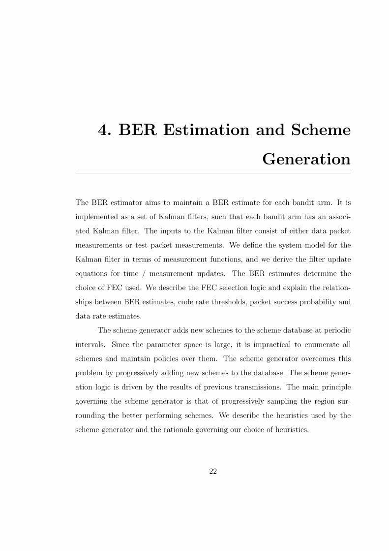
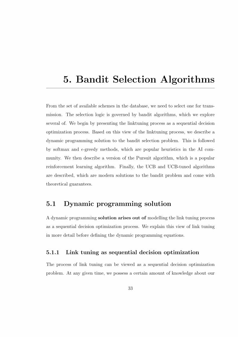
1. We draw schemes from a probability density function (PDF) curve, which we
modify as time progresses. Fig. 4.4 illustrates the evolution of the PDF for
an example parameter. Each parameter has its own PDF.
28

We manipulate the shape of the PDF for each parameter independently, even
though in reality the PDFs of the parameters are likely not independent.
Doing so is acceptable because we do not know the relationship between the
PDF’s of parameters. Given the absence of any way to easily deduce these
relationships, we treat the PDFs independently. That way, we retain the
option to sample schemes in all directions.
2. In the beginning, the schemes are drawn from a uniform distribution. This
meets the first requirement, i.e., we consider the parameter space in its en-
tirety. We draw d1 schemes and store them in the database initially.
3. After d2 transmissions, new schemes are generated. We determine which
scheme has the maximum expected data rate among the ones that were tried.
We refer to this scheme as the winning scheme.
4. We then add d3 schemes to our database. These schemes are drawn from
a discrete PDF, which is based on the normal distribution and centered at
the winning scheme. Drawing schemes from such a distribution allows us to
meet the second and third requirements: we now have higher probability of
sampling points closer to the previously successful schemes. Changing the
standard deviation of the normal curve provides us with a mechanism to
control the probability with which the newly generated schemes lie close to
the previously successful ones.
5. This discrete distribution is defined for each modem parameter. It has a
support equivalent to the valid range of parameter values. The distribution
defines a probability for selecting a given modem parameter value. We need to
define a discrete distribution instead of using the normal distribution directly
because modem parameter values are discrete and have finite support.
29

6. The discrete distribution is defined as follows. Suppose we have an integer
valued modem parameter y 2 [a, b], and we derive our discrete distribution
based on a normal PDF with mean ⇠ and standard deviation �. Probability
p(yi
) of selecting a value y
i
is given by:
p(yi
) =
8>>>>>>><
>>>>>>>:
1Z
x
i
+0.5Rx
i
�0.5
�(y; ⇠, �)dx a < x
i
< b
1Z
bR
b�0.5
�(y; ⇠, �)dx x
i
= b
1Z
a+0.5Ra
�(y; ⇠, �)dx x
i
= a
(4.15)
where �(y; ⇠, �) is the normal PDF and Z is a normalizing factor:
�(y; ⇠, �) =1
�
p2⇡
e
� (x�⇠)2
2�2 (4.16)
Z =
bZ
a
�(y; ⇠, �)dy (4.17)
7. If all the previously tried schemes have an estimated data rate of zero, we
draw again from the uniform distribution.
8. Suppose one of the parameters can take values between 0 and 100, and the
winning scheme had the value of this parameter = 75 We then generate dis-
crete PDF based on a normal distribution with mean = 75. Also, 75 divides
this range in two intervals: [0, 74) and [75, 100]. We set the standard devi-
ation of the normal curve to be half the range of the smaller interval, i.e.,
(100 � 75)/2 = 12.5. At every d2 transmissions it is time to generate new
schemes again. At this point, we multiply the standard deviation by a shrink
factor d
f
2 (0, 1).
We set d1 = 10, d2 = 6, d3 = 3 and d
f
= 0.9. The choice of using a normal
distribution, the method we use for setting its standard deviation, as well as the
values of d1, d2, d3 and d
f
are heuristics based on our experience:
30
0 20 40 60 80 100
0 20 40 60 80 100
prob
0 20 40 60 80 100param value
Figure 4.4: Evolution of probability density curves used by scheme generator
31

1. If d2 is too large and none of the schemes in the database are performing well,
then we have to wait for a long time before exploring any new schemes. If d2
is too small, then we end up generating new schemes too fast. A value of 10
works well in practice.
2. If d3 is set to be much larger than d2, then we end up accumulating too many
schemes that never get tried. Hence, our choice of value for d3 is primarily
guided by memory constraints.
3. The tuner performance is not very sensitive to d1.
4. d
f
controls the rate at which we narrow width of our normal distribution, and
we have found that a value of 0.9 works well in practice.
5. Setting the standard deviation of the normal curve to be equal to half of the
smaller interval between the mean and the extreme values of the parameter
makes the curve more symmetric about the mean.
32
5. Bandit Selection Algorithms
From the set of available schemes in the database, we need to select one for trans-
mission. The selection logic is governed by bandit algorithms, which we explore
several of. We begin by presenting the linktuning process as a sequential decision
optimization process. Based on this view of the linktuning process, we describe a
dynamic programming solution to the bandit selection problem. This is followed
by softmax and ✏-greedy methods, which are popular heuristics in the AI com-
munity. We then describe a version of the Pursuit algorithm, which is a popular
reinforcement learning algorithm. Finally, the UCB and UCB-tuned algorithms
are described, which are modern solutions to the bandit problem and come with
theoretical guarantees.
5.1 Dynamic programming solution
A dynamic programming solution arises out of modelling the link tuning process
as a sequential decision optimization process. We explain this view of link tuning
in more detail before defining the dynamic programming equations.
5.1.1 Link tuning as sequential decision optimization
The process of link tuning can be viewed as a sequential decision optimization
problem. At any given time, we possess a certain amount of knowledge about our
33

schemes and their performances in the channel. We can think of possessing this
knowledge as equivalent to being in a certain state. Given this state, we need to
make a decision and choose a scheme. Receiving the results of the transmission
allows us to update our state, and then it’s time to make the decision again.1 Thus
the link tuning process is essentially a decision process. We wish to optimize our
decisions to maximize the average data rate. Note that maximizing the average
data rate requires us to optimize the entire series of decisions, rather than any
particular decision in isolation.
Dynamic programming is an algorithmic paradigm that is well suited to solve
problems of this nature [34]. We shall now illustrate how dynamic programming
works. Consider an environment where we can transition from state ⇠
t
at time t to
T (⇠t
, a) = ⇠
t+1 by choosing an action a. T (⇠t
, a) is a function that describes the state
transitions. Choosing action a yields an immediate reward. The expected value of
immediate rewards are given by a reward function R(⇠t
, a). The key idea of dynamic
programming lies in computing the value function V (⇠t
). The value function is a
measure of the inherent goodness of that state. The optimal value function V
⇤(⇠t
)
describes the maximum total expected reward looking into the future. The optimal
value function can be computed by the following recursive definition:
V
⇤(⇠) = arg maxa
{R(⇠t
, a) + V
⇤(T (⇠t
, a))} (5.1)
Equation (5.1) is known as the Bellman optimality equation in literature [34].
We now proceed to describe how to compute the optimum value function for the
link tuner and describe a bandit selection policy based on it. Note that we do not
have an explicit expression for T (⇠, a) in the context of the link tuner, and instead
compute it implicitly.
1The feedback mechanism is assumed to be reliable. In practise, this is achieved by usinga reliable (but low data rate) scheme for exchanging control data. Errors in the feedback willa↵ect our BER estimates. The Kalman filter constructed in chapter 4 is designed to handle noisymeasurements and smoothes these errors over time.
34

5.1.2 Dynamic programming equations
Let the data rate, packet success probability estimate and bit error rate estimate for
scheme i (which is associated with arm j and error coding scheme c) at current time
t be µ̂
i,t
, ↵̂(j,c),t and ✓̂
j,t
. Note the correspondence between i and (j, c). We define
the state ⇠
t
to consist of the 3-tuple (↵̂(j,c),t, �j
, r
c
). Choosing an action corresponds
to transmitting a packet s
pi
.The immediate expected reward is given by the function
R(⇠t
, s
pi
):
R(⇠t
, s
pi
) = ↵̂(j,c),t�j
r
c
(5.2)
Given the results of transmitting packet s
pi
, we use the equations in sec-
tion 4.1.2 to compute the new state ⇠(t+1)|spi
. To compute ⇠(t+1)|spi
, we only need to
update ↵̂(j,c),t since �
j
and r
c
don’t change with time. To update ↵̂(j,c),t, we first up-
date ✓̂
j
using the Kalman filter equations in section 4.1.2, followed by Equation (4.1)
to update ↵̂(j,c),t.
Given that we transmitted s
pi
, updating ↵̂(j,c),t is conditioned on a successful
/ failed reception of s
pi
. Since failed receptions yield zero reward, we only need to
compute the update conditioned on successful reception, and multiply that by the
probability of successfully receiving s
pi
. Putting all of this together, we arrive at
the following expression for the optimal value function for scheme i in state ⇠
t
:
V
⇤i
(⇠t
) = arg maxj,c
(R(⇠
t
) +X
c2C
↵̂(j,c),tV⇤i
⇣⇠(t+1)|sp
i
⌘)(5.3)
We define the following policy based on the optimal value function. At each
time step, we choose the scheme i that maximizes V
⇤i
(⇠t
):
j(t) = arg maxi
V
⇤i
(⇠t
) (5.4)
35

5.2 Softmax Exploration
Softmax exploration is a heuristic which computes probabilities for each scheme [14].
The probability of picking a scheme is proportional to its expected reward. Thus,
arms with greater empirical reward expectations are picked with higher probability.
Let µ̂
i
(t) be the expected data rate of scheme i at time t. p
i
(t), the probability of
choosing scheme i at time t is given by:
p
i
(t + 1) =e
µ̂
i
(t)/⌧
Pi
e
µ̂
i
(t)/⌧(5.5)
where ⌧ is a temperature parameter. When ⌧ = 0, the heuristic exhibits pure
greedy behaviour. As ⌧ tends to infinity, the algorithm picks schemes uniformly at
random. One could possibly use decreasing ⌧ schedules, but [35] show empirical
evidence that such schedules o↵er no practical advantages, so we choose a fixed
value of ⌧ = 0.1 for our experiments.
5.3 ✏-greedy
The ✏-greedy is a commonly used heuristic in the AI community [36]. It is very
simple and well suited for use in sequential decision problems. Given its widespread
use and adoption, we implement a version in the link tuner. The probability of
choosing a scheme i at time t is given by:
p
i
(t + 1) =
8<
:1 � ✏ + ✏/k if i = arg max
i
µ̂
i
(t)
✏/k otherwise(5.6)
One could possibly vary ✏ adaptively. However, [35] presents empirical ev-
idence that finds no practical advantage in doing so. In our experiments we find
that a value of 0.05 works well, so we use that for our experiments.
36

5.4 Pursuit algorithm
Pursuit algorithms maintain a policy over each bandit arm, the updates to which
depend on the estimated reward of the arm. We use a version of the pursuit
algorithm as described in [14]. Each scheme is assigned a uniform probability of
selection, p
i
(t) = 1/|S|. The probabilities are updated as per:
p
i
(t + 1) =
8<
:p
i
(t) + (1 � p
i
(t)) if i = arg maxi
µ̂
i
(t)
p
i
(t) + (0 � p
i
(t)) otherwise(5.7)
where 2 (0, 1) is the learning rate. We have found that = 0.9 generally works
well, so we use that value for our experiments.
5.5 Upper Confidence Bounds (UCB)
The UCB family of algorithms are regarded as the state-of-the-art algorithms that
solve the multi armed bandit problem. These algorithms were proposed by [28].
Unlike ✏-greedy and softmax methods, these algorithms are based on sophisticated
mathematical ideas and come with strong theoretical performance guarantees. We
use 2 versions of the UCB family of algorithms: the UCB1 and the UCB1-tuned.
5.5.1 UCB1
The simpler algorithm, UCB1, maintains a count of the number of times scheme
n
i
(t) scheme i was chosen. Initially, each scheme is played once. Subsequently at
round t, the algorithm chooses scheme i as per:
j(t) = arg maxi
µ̂
i
+
s2 ln t
n
i
(t)
!(5.8)
37

5.5.2 UCB1-Tuned
UCB1-Tuned is an alternate version of the algorithm proposed by the authors
in [28]. It can have better performance in practise, but it comes without theoretical
guarantees. The main feature of the UCB1-Tuned is that it accounts for the variance
of each scheme in addition to the expected reward. The schemes are chosen as per:
j(t) = arg maxi
µ̂
i
+
s2 ln t
n
i
(t)min(
1
4, V
i
(ni
))
!(5.9)
where
V
i
(t) = �̂
2i
(t) +
s2 ln t
n
i
(t)(5.10)
�̂
2i
(t) is computed from the empirical sum of squares of µ̂
i
.
38

6. Results
We conducted comparative performance tests with a simulation setup, a water tank,
and at the Republic of Singapore Yacht Club (RSYC). We first describe the test
setup, present the results of our tests and finish with a short summary of results.
6.1 Test setup
We compare the performance by varying the bandit selection algorithm used and
plotting the average data rate. The x-axis of each plot represents time in terms of
the number of packets transmitted. The y-axis represents the average data rate at
that time instant. All data rates reported are user data rates, i.e., the total number
of user data bits recieved divided by time. Each test was performed by establishing
a single point-to-point communication link. Note that in practise, running such a
test necessitates the use of a handshake protocol. For example when we switch to
a new scheme, a control packet exchange is necessary in order to ensure that both
modems have switched to the correct scheme.
The handshake protocol imposes a time overhead of the order of a 2-way
propagation delay for every control packet exchange. Optimizing the protocol over-
head is essential for obtaining high data rates. In particular, an underwater channel
presents many opportunities for such optimization since one can exploit the large
propagation delay time. See [37] and [38] for examples of such optimizations. How-
39

0 5 10 15 20 25 30 35 40transmission no
0
2
4
6
8av
gda
tara
te(k
bps)
DPsoftmax
ucbUcbTuned
pursuitegreedy
Figure 6.1: Average data rate in simulation
ever protocol optimization is not the focus of this thesis. Hence, all the results
presented in this chapter do not account for the protocol overhead. 1
6.2 Simulation results
The majority of the tests over the course of the link tuner development were carried
out on a simulator. The simulator tries to simulate an water tank environment.
The simulator is a random forest regressor trained with data consisting of various
schemes and the resulting BER as observed in a water tank [22]. In order to train
the regressor, we transmitted 3,546 schemes in the tank and recorded the uncoded
BER. The regressor learns a function mapping from schemes to BER, and provides
1The time overhead is caused by the handshake protocol. Since protocol optimization is notwithin the scope of this thesis, we do not account for the protocol overhead in our results. Sincethe protocol overhead is not accounted for, setting an upper limit on it is unnecessary.
40

0 5 10 15 20 25 30 35 40transmission no
0
2
4
6
8
10
12in
stan
tane
ous
data
rate
(kbp
s)instantaneous data rate (simulation)DPsoftmax
ucbUcbTuned
pursuitegreedy
Figure 6.2: Instantaneous data rate observed in simulation
us with a BER estimate when presented with a scheme. In order to estimate the
accuracy of the regressor, we performed a 5 - fold cross validation test. The data
was randomly split between training (80 %) and test (20 %) sets. The regressor
was trained on the training set, and its coe�cient of determination was measured
on the test set. The process was repeated 5 times, and the mean of the coe�cient
of determination was found to be 0.98, with a standard deviation of 0.45%.
Fig. 6.1 plots the average data rate attained in simulation. From the figure,
we can see that the dynamic programming method attains the highest average data
rate, followed by pursuit and softmax. UCB, UCB-tuned and ✏-greedy have similar
performance characteristics. In order to give the reader a sense of the exploration
and exploitation process undertaken by the tuner, we also plot the instantaneous
data rates. Fig. 6.2 plots the instantaneous data rates measured in the simulation
run. As in the previous plot, the x-axis represents time in terms of the number of
41

packets transmitted. The y-axis is the data rate measured for that packet. 2
In Fig. 6.2 the dynamic programming (DP) method first starts o↵ with a
data rate of zero at time zero, followed by two packets with data rates of around
4.5 kbps, followed by data rates of around 8 kbps for the rest of the test. The data
rate drops to zero periodically, and that corresponds to the decreases in the average
data rate curve for the DP method in Fig. 6.1.
The softmax method mostly yields data rates of around 3.5 kbps, but also
keeps dropping to zero periodically. The rest of the methods have similar behaviour,
except their data rates do not drop to zero as often. The instantaneous data rate
dropping to zero can be caused by: a) the tuner trying a new scheme that did not
succeed, b) the tuner transmitted a test packet (all test packets have a data rate
of zero), 3 or c) the bit error rate increased beyond the error correction capability
of the FEC in use.
6.3 Watertank tests
Fig. 6.3 shows the performance of the tuner in a water tank. The tank measures
2⇥2⇥2 meters. The modems were placed at diagonally opposite ends at depths
of 0.5 meters. We can see that the dynamic programming algorithm has the best
average data rate performance.
Fig. 6.4 shows the average data recorded at the end of the tank test. The
average data rate of the dynamic programming method exceeds the rest by 4 kbps.
2The time instances when the data rate is zero correspond to dropped packets. Packets getdropped when the channel BER is greater than the BER threshold of the scheme. The zerodata rate points correspond to instances when the BER turned out to be greater than the BERthreshold for the schemes chosen by the DP algorithm.
3The decision to transmit a test packet hinges on the state of the BER estimator, the schemegenerator and the bandit selection algorithm. Transmitting test packets has an e↵ect on band-width e�ciency and utilization. However these e↵ects have been fully accounted for in all oursimulation as well as field trial results. Specifically, have counted the time spent in transmittingtest packets while reporting all instantaneous as well as average data rate results.
42

0 5 10 15 20 25 30 35 40transmission no
0
2
4
6
8
10
12av
gda
tara
te(k
bps)
DPsoftmax
ucbUcbTuned
pursuitegreedy
Figure 6.3: Average data rate in tank
✏-greedy, pursuit, UCB-tuned, and UCB methods have average data rates between
2 to 3 Kpbs. The lowest average data rate is recorded by the softmax method. As
a benchmark, we also include the data rate of the default scheme (without tuning).
The data rate yielded by the default scheme is 0.345 kbps. All methods yield data
rates that are at least twice the default.
6.4 Test at RSYC
Fig. 6.5 shows the location of the RSYC test site as map snapshot. The dark red
line indicates the point-to-point communication link established for the test. The
RSYC is a marina which provides docking facilities for a number of yachts and
boats. It is located next to the West Coast ferry terminal. The ferry terminal
provides ferry services to a number of o↵shore facilities. The presence of nearby
43

default softmax ucb UcbTuned pursuit egreedy DP0
1
2
3
4
5
6
7
8av
gda
tara
te(k
bps)
Figure 6.4: Average data rate in tank at end of test
Figure 6.5: RSYC test site
44

0 5 10 15 20 25 30 35 40transmission no
�1
0
1
2
3
4
5
6
7av
gda
tara
te(k
bps)
DPsoftmax
ucbUcbTuned
pursuitegreedy
Figure 6.6: Average data rate at RSYC
boating activities makes the channel a very noise one to operate in. The water
depth at RSYC is very shallow (6 to 7 meters on average). Both modems were
deployed at a depth of 1.5 meters. Fig. 6.5 shows the location of the modems at
the test site. The boating activity together with shallow depths provide us with a
very challenging environment to operate in.
Fig. 6.6 shows the average data rates recorded at RSYC. We can see that the
dynamic programming method has the highest average data rates for most of the
test duration. This is followed by the ✏-greedy, UCB-tuned and softmax methods.
The pursuit and UCB methods have nearly identical as well as the lowest average
data rates.
Fig. 6.7 shows the average data rate measured at the end of the test. We can
benchmark our results by comparing against the data rate o↵ered by the default
scheme (without any tuning). The default scheme o↵ers a data rate of 0.345 kbps.
45

default ucb pursuit softmax UcbTuned egreedy DP0
1
2
3
4
5av
gda
tara
te(k
bps)
Figure 6.7: Average data rate at RSYC at end of test
By comparision, the average data rate of the tuner using the dynamic programming
method is 4.7 kbps, representing a 13-fold increase. The lowest average data rate
attained by the pursuit method is 1.06 kbps, which is 3 times the default data rate.
Fig. 6.8 shows the instantaneous data rate for the tests at RSYC. In comparision
with Fig. 6.2, Fig. 6.8 looks more chaotic in the sense that each method experiences
more variation in the instantaneous data rates. This is a likely reflection of the more
dynamic, and constantly changing nature of the RSYC enviroment in contrast to
a simulated water tank.
6.5 Summary of results
The average data rate at the end of the simulation and watertank tests range from
1 to 7 kbps, depending on the bandit selection algorithm used. For both tests, the
46

0 5 10 15 20 25 30 35 40transmission no
0
2
4
6
8
10
12in
stan
tane
ous
data
rate
(kbp
s)instantaneous data rate (rsyc)
DPsoftmax
ucbUcbTuned
pursuitegreedy
Figure 6.8: Instantaneous data rates observed at RSYC
dynamic programming method attains the highest average data rate. The average
data rates at the end of the RSYC test range from 1 to 4.7 kbps, depending on
the bandit selection algorithm used. In contrast, the default data rate (without
tuning) is 0.345 kbps. Again, the dynamic programming method has the highest
average data rate. The RSYC is a fairly challenging environment due to extremely
shallow water depths (around 1.5 meters) and noise generated by boating activity in
the vicinity. The dynamic programming method attains data rates that far exceed
other methods in a more forgiving environment such as a watertank. In contrast,
the average data rate curves for the RSYC test are much closer to each other. In
harsher environments such as RSYC, the ceiling for the maximum attainable data
rate drops considerably. This suggests that other parts of the linktuner (the scheme
generation process and the BER estimator) pay a relatively more important part
in the tuning process in such environments.
47

7. Analysis and Interpretation of
Results
We aim to give the reader some insight into the process of link tuning. Over
the course of the link tuning process, we dynamically add new schemes from the
available search space. We then use one of the bandit arm selection algorithms to
choose which scheme to use for transmission. Subsequent sampling is informed by
the history of results from previous transmissions.
Fig. 7.1 plots the sampling and selection process for one of the parameters,
namely the number of carriers in an OFDM symbol. The x-axis represents time
in terms of the number of transmissions. The y-axis is the value of the number
of carriers. We have 5 choices for this parameter (64, 128, 256, 512, 1024). The
blue dots correspond to the values that were sampled and added to our collection
of schemes. The red dots represent the values that were selected for transmission.
This plot was generated using link tuning data in a water tank environment with
the dynamic programming bandit selection algorithm.
We can see that the tuner begins by adding schemes with all 5 possible
choices in its set of available schmes. At the very early stages, it selects a di↵erent
parameter value each time. Soon after this early stage, it selects the value 1024
for the vast majority of the rest of the tuning session while occassionally sampling
/ selecting 512. The blue and red dots overlap in the 1024 band. Note that even
48

Figure 7.1: Evolution of number of carriers sampling and selection (simulation)
Figure 7.2: Evolution of prefix length sampling and selection (simulation)
49

though the tuner uses a value of 1024 for most of the tuning session, it occassionally
switches back-and-forth between 1024 and 512. This behaviour is reflective of a fine
tuning process, which occours after the tuner has already determined that a value
of 1024 performs well.
The tuner changes the values of all parameters simultaneously. Let us ex-
amine Fig. 7.2, which plots the sampling / selection history for another parameter:
the prefix length of an OFDM symbol. The x-axis represents time in terms of the
number of transmissions. The y-axis is the value of the prefix length. Most of
the selected values (i.e., the red dots) hover at around 256 in the beginning (until
transmission # < 30). The selected values then begin to drop in the region where
transmission # 2 (30, 100). They finally settle at values close to zero for transmis-
sion # > 100. We can see that for transmission # < 100, the selected values are
turbulent, which is reflective of the exploratory behavior of the tuner in that phase.
The sampled values (i.e., the blue dots) follow a similar trend to the selected
values: we can see that the sampled values are clustered around the selected values.
In the beginning (until transmission # < 100), the range of sampled values is
comparatively large. Again, this is reflective of the exploratory behavior of the
tuner. In the transmission # > 100 region, the certainty in our knowledge increases.
This is reflected in the comparatively narrow range of sampled values in this region.
One can interpret the tuner behavior in the transmission # < 100 region as a coarse
tuning process, as compared to the fine tuning in the transmission # > 100 region.
The above described sampling and selection process occurs simultaneously
across all parameters. Information is shared between the sampling and selection
processes, and they drive each other. Besides prefix length and number of carriers,
here are the other tunable parameters in the UNET-II modem implementation,
along with the range of values they can take:
1. Modulation mode (coherent or incoherent)
50

Figure 7.3: Link tuning represented as a graph (water tank data, DP algorithm)
51

Figure 7.4: Node ID versus the number of times the node was tried (+1)
2. Di↵erential mode (time or frequency)
3. QPSK or BPSK modulation
4. Su�x length (0 to 1024)
5. Number of nulls (0 to 1024)
6. Error correction type (Convolution, Golay, both or none)
In order to visualize such a multi-dimensional process, we use a directed
graph representation of the tuning process. The sampled and selected schemes tend
to cluster in regions yielding better data rates. One can observe that some nodes
in the graph are more prominent than others: these nodes are selected relatively
more frequently and new nodes in their neighbourhood are sampled. A graph
representation also allows us to better check that the tuner has indeed considered
all of the available search space. Note that we don’t need the tuner to have selected
52

schemes located all over the search space: that would result in a highly ine�cient
tuner. We do however, need to verify that all major regions of the search space were
sampled at some point of the tuning process. That way we know that no part of
the available space was discarded. We use a combination of a graph representation
along with some plots to do so.
7.1 Evolution and clustering of schemes
The nodes in our graph correspond to schemes. If the tuner selects scheme 2 now,
and the previously selected scheme was 1, then we add an edge to the graph from
node 1 to 2. If the tuner selects scheme 1 twice in a row, then we add a self edge to
node 1. The scheme generator generates new schemes in the vicinity of the winning
scheme. This is represented in the graph by an edge from the winning scheme to
the new scheme that was generated. Fig. 7.3 shows the graph that was generated
from a run of the link tuner in the water tank using the dynamic programming
algorithm. The node sizes are proportional to the degree, where the degree of a
node is the number of edges incident on it. The set of nodes has been partitioned
according to the number of times each node was selected for transmission. The
node colors were assigned to match this partitioning. For example, all the nodes
which have no edges incident on them were never selected, and hence they share
the same same color.
One of the features that stand out about the graph in Fig. 7.3 is that nodes
52, 20 and 9 are dominant. Fig. 7.5, Fig. 7.6 and Fig. 7.7 show the ego networks of
the graph centered at nodes 52, 20 and 9 respectively. An ego network centered at
a given node is a subgraph where all nodes are at a 1-hop distance from the center
node. From Figures 7.5, 7.6 and 7.7 it is evident that nodes connected to 52, 20
and 9 consist of the majority of the total nodes in the graph.
Fig. 7.4 plots the number of times a given node was selected plus one. (The
53

Figure 7.5: Ego network centered at node 52
54

Figure 7.6: Ego network centered at node 20
55

Figure 7.7: Ego network centered at node 9
56

addition of one is in order to accommodate a logarithmic scale on the y-axis). From
the figure, we see that most of the nodes were tried once. The second biggest group
of nodes correspond to the schemes that were generated and added to our collection,
but never selected for transmission. Finally, there are a few nodes that were tried
more than once. Of these, we can see that nodes 52 and 20 have the maximum
frequency of selection.
The tuner starts with an initial collection of schemes that are located far
apart in the search space. One can think of this as coarse tuning. Once it finds a
scheme that performs well, it generates new schemes in the vicinity of the winning
scheme. One can think of this as fine tuning. The scheme generation process
continues until the tuner finds schemes that perform better. When this process
is represented as a graph, some nodes nodes dominate, and one can conceptually
think of such nodes as hub nodes. Figures 7.5, 7.6, 7.7 and 7.4 are illustrative of
these characteristics.
Finally, it would be interesting to see the evolution of the graph over time.
Fig. 7.8 shows snapshots taken over the course of the evolution of the final graph.
The snapshots are in chronological order. They are placed in clockwise direction,
starting from the top left corner. The node sizing and coloring rules are the same
as those for Fig. 7.3.
The first snapshot was taken at the initialization. At this point, we only have
a set of 11 schemes in our collection. Out of those, we have only selected scheme 4
for transmission. The second snapshot was taken shortly after initialization. The
red nodes were tried more often than the green ones in this snapshot. We also see
that node 9 has emerged as a hub node in this graph: it has the most number of
edges incident on it, and it is also the only node with self-edges. The tuner often
alternated between trying a new scheme such as 4, 2, 1 etc. and going back to
selecting scheme 9. This behavior generates the many edges that go from other
57

initialization
Node 9 emerges as a hub node
Nodes 15, 20, 22 may emerge as hubs
By the halfway mark, nodes 9, 20 and 52 are established as hubs
Figure 7.8: Evolution of the graph in Fig. 7.3
58

nodes and terminate at node 9, and is indicative of the balance the tuner is trying
to balance exploration versus exploitation.
The third snapshot continues this trend and we can see nodes 15, 20, and
22 gain prominence. The fourth snapshot was taken at the midway mark. By this
time, nodes 52, 20 and 9 have been well established as hub nodes. We can also
see that the graph tends to grow in clusters centered around the hub nodes. The
clustering e↵ect is a result of the scheme generator which generates new schemes in
the vicinity of the ones that have been found to perform well. We can also see the
group of purple nodes, which correspond to schemes that exist in our collection but
were never selected for transmission. This growth pattern continues and eventually
yields the graph shown in Fig. 7.3.
7.2 Visualizing RSYC trial data
We use a di↵erent node coloring scheme for this section in order to illustrate that
the tuner sampled schemes that were reasonably spread out all around the search
space. Fig. 7.9 shows a graph representation of the tuning process. The tuning data
for this graph was generated by tests at RSYC, and use the dynamic programming
bandit selection method. This graph looks di↵erent compared to Fig. 7.3, because
we use a di↵erent graph layout algorithm to render this graph for visual clarity
reasons.
The nodes are coloured as their scheme type. We define 6 di↵erent scheme
types, depending on the values of the following parameters:
1. Modulation type (coherent or incoherent)
2. Di↵erential mode (time or frequency di↵erential)
3. BPSK or QPSK
59

Figure 7.9: Graph representation of link tuning data (RSYC data, DP algorithm)
60

scheme type modulation type di↵erential mode BPSK/QPSK1 incoherent - BPSK2 incoherent - QPSK3 coherent time BPSK4 coherent time QPSK5 coherent frequency BPSK6 coherent frequency QPSK
Table 7.1: Mapping from scheme type to modulation parameters for nodes in Fig-ure 7.9
Table 7.1 lists the mapping from scheme type to values of the above mod-
ulation parameters. Note that for scheme types 1 and 2, the di↵erential mode
parameter is not applicable since they use incoherent modulation. Fig. 7.10 lists
the correspondence between node color, scheme type and the percentage occurrence
of scheme type in the graph in Fig. 7.9. The node labels correspond to code rate
of the FEC used for that scheme, except for the ones labelled 0.0 (those nodes cor-
respond to test packet, and the label 0.0 was chosen to indicate that a test packet
does not carry any user data.)
We can see that all 6 scheme types are represented in the graph. Types 5 and
6 constitute the largest share (57.98%). That means most of the schemes sampled
in the tuning process were coded with coherent modulation, operated in frequency
di↵erential mode, and switched between BPSK or QPSK.
The node labels show that a mixture of test and data packets were sampled.
For data packets, we have 3 choices of FEC implementations on the UNET-II
modem. They have code rates of 0.5, 0.3 and 0.15 respectively. We can see nodes
with code rates of 0.3 and 0.15. However, there is no node with a label of 0.5.
This can be explained by considering the FEC selection logic in the link tuning
architecture. Recall that the tuner chooses an FEC for a given scheme by getting
BER estimates for that scheme. The BER estimates are provided by a Kalman
filter based estimator. In order to choose an FEC with code rate 0.5, the scheme
61
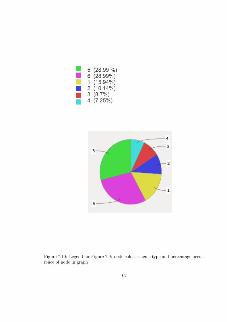
5 (28.99 %)6 (28.99%)1 (15.94%)2 (10.14%)3 (8.7%)4 (7.25%)
Figure 7.10: Legend for Figure 7.9: node color, scheme type and percentage occur-rence of node in graph
62

Figure 7.11: Evolution of number of carriers sampling and selection (RSYC data)
Figure 7.12: Evolution of prefix length sampling and selection (RSYC data)
63

needs an to have an estimated (uncoded) BER of less than 4%. It turns out that
none of the schemes sampled in the RSYC tests had an estimated BER of less than
4%, hence we don’t see any node labelled 0.5.
Fig. 7.11 shows the evolution of the sampling and selection process for the
parameter number of carriers. A blue dot indicates a sampled scheme, while a red
dot indicates a scheme selected for tranmsission. We have 5 choices for values of
this parameter: 64, 128, 256, 512 and 1024. We can see that all values were sampled
at some point in time. We can also see that 512 and 1024 are the dominant values
for this parameter.
Fig. 7.12 shows the evolution of the sampling and selection process for the
parameter prefix length. We have 1024 possible values for this parameter, ranging
from 0 to 1023. Values ranging from 8 to 352 were sampled at various points in
time. We can see that the sampled as well as selected values follow a general,
though somewhat chaotic downward trend, similar to Fig. 7.2. The prefix length is
one of the measures of overhead in a given OFDM symbol: higher the prefix length,
more the overhead. Thus, the downward trend in prefix length values reflects the
increase in average data rate over time.
7.3 Summary
A variety of visualizations were generated with the aim of providing insight into
the link tuning process. We showed how information is shared between the sam-
pling and selection process and how they drive each other. Illustrative plots of
the sampling and selection process were generated for two modem parameters. In
order to visualize the sampling and selection process across all modem parameters
simultaneously, a graph representation of the link tuning process was formulated.
Rendering the graph representation allowed us to visualize the evolution and clus-
tering phenomena of schemes over time. In order to verify that the tuner considers
64

the search space in its entirety, we generated a slightly di↵erent graph representa-
tion of link tuning data from the RSYC experiments. This representation confirmed
that the sampled schemes were reasonably spread out over the entire search space.
65

8. Conclusion
8.1 Summary of contributions
1. A family of learning algorithms to tune an underwater communication link
are derived.
2. A data driven approach to link tuning is pursued, leading to the development
of a tuner that works with any modem implementation, and requires only bit
error rate information.
3. Results from performance tests in: a) simulation, b) water tank, and c) field
trials at RSYC demonstrate a significant improvement in average data rates.
4. An extensive analysis and discussion of results is presented in order to provide
insight into the mechanism of link tuning.
8.2 Conclusion
Link tuning algorithms to tune a point to point underwater communication link
were presented. The link tuner is data driven and needs only bit error informa-
tion as input. Hence, the link tuner is independent of the modem implementation
and is useful even as the underlying physical layer implementation changes and
66

evolves. Online mechansims for link tuning were developed, allowing us to contin-
uously update modem parameter values for di↵erent channels. The online tuning
mechanism also allows the tuner aims to maximize for the average data rate, rather
than search for the maximum possible data rate. The link tuner was implemented
on the UNET-II modem. Results from simulation, tank tests and field trials at
RSYC were presented. In all cases, using the tuner resulted in improved average
data rate when compared with the default data rate without tuning. At RSYC,
average data rates between 1 to 4.7 Kbps were recorded, depending on the bandit
selection algorithm used. In comparison, the default data rate without tuning is
345 bps. Finally, a number of visualizations are presented in order to provide the
reader with insight and intuition into the process of link tuning.
8.3 Further research
The link tuner can be enhanced by augmenting it with physical models that describe
the properties of a given modem implementation. Future research into building
physics based models of interactions between the underwater channel and commu-
nication signals would involve investigation of acoustic propagation models as well
as the design of custom signals that can allow us to infer key properties of the under-
water channel. Ultimately, a hybrid approach that combines data driven techniques
along with physics based models customized for a given modem implementation can
lead to even better data rate performance.
67
Bibliography
[1] M. Chitre, S. Shahabudeen, L. Freitag, and M. Stojanovic, “Underwater acous-
tic communications and networking: Recent advances and future challenges,”
in Proceedings of Oceans 2008, vol. 42, no. 1. Marine Technology Society,
2008, pp. 103–116.
[2] M. Stojanovic, “Recent advances in high-speed underwater acoustic commu-
nications,” IEEE Journal of Oceanic Engineering, pp. 125–136, 1996.
[3] B. Benson, Y. Li, R. Kastner, B. Faunce, K. Domond, D. Kimball, and
C. Schurgers, “Design of a low-cost, underwater acoustic modem for short-
range sensor networks,” in Proceedings of Oceans, 2010, pp. 1–9.
[4] M.Suzuki and T.Sasaki, “Digital acoustic image transmission system for deep
sea research submersible,” in Proceedings of Oceans, vol. 2, 1992, pp. 567–570.
[5] G. H. et. al., “Subsea remote communications utilising an adaptive receiving
beamformer for multipath suppression,” in Proceedings of Oceans, vol. 1, 1994,
pp. I/313–I/316 vol.1.
[6] L. Freitag, M. Grund, S. Singh, J. Partan, P. Koski, and K. Ball, “The WHOI
micro-modem: An acoustic communcations and navigation system for multiple
platforms,” in Proceedings of Oceans, 2005, pp. 1086–1092 Vol. 2.
i

[7] M. Chitre, I. Topor, and T. Koay, “The UNET-2 modem - an extensible tool
for underwater networking research,” in Proceedings of Oceans, 2012, pp. 1–7.
[8] K. G. Kebkal, R. Bannasch, A. G. Kebkal, and S. G. Yakovlev, “Ultrasonic
link for improved incoherent data transmission in horizontal shallow water
channels,” in Proceedings of Oceans, vol. 4, 2003, pp. 1786–1792 Vol.4.
[9] M. Chitre, “Underwater acoustic communications in warm shallow water chan-
nels,” Ph.D. dissertation, National University of Singapore, pp. 16-20, 2006.
[10] R. Urick, Principles of Underwater Sound. McGraw Hill, 1983.
[11] J. Preisig, “Acoustic propagation considerations for underwater acoustic
communications network development,” in ACM SIGMOBILE Mobile
Computing and Communications Review. New York, NY, USA: ACM, 2007,
pp. 2–10. [Online]. Available: http://doi.acm.org/10.1145/1347364.1347370
[12] M. Porter and M. Siderius, “Acoustic propagation in very shallow water,” in
Waterside Security Conference (WSS), 2010 International, 2010, pp. 1–4.
[13] P. Barley, H. Bucker, J. Rice, M. Green, and J. Woxstroem, “Acoustic commu-
nication channel modeling for the baltic sea,” in Proceedings of Oceans, vol. 3,
1999, pp. 1504–1511 vol.3.
[14] R. S. Sutton and A. G. Barto, Reinfocement Learning: An Introduction. MIT
Press, 1998.
[15] S. Gao, L. Qian, D. Vaman, and Q. Qu, “Energy e�cient adaptive modulation
in wireless cognitive radio sensor networks,” IEEE International Conference
on Communications, pp. 3980–3986, 2007.
ii

[16] P. Tan, Y. Wu, and S. Sun, “Link adaptation based on adaptive modulation
and coding for multiple-antenna OFDM system,” IEEE Journal on selected
areas in communications, no. 8, pp. 1599–1606, 2008.
[17] F.Peng, J.Zhang, and W. Ryan, “Adaptive modulation and coding for IEEE
802.11n,” in Wireless Communications and Networking Conference, 2007, pp.
656–661.
[18] C. Pandana, Y. Sun, and K. J. R. Liu, “Channel-aware priority transmission
scheme using joint channel estimation and data loading for OFDM systems,”
IEEE Transactions on Signal Processing, vol. 53, no. 8, pp. 3297–3310, 2005.
[19] Y. Jing and X. Yu, “ML-based channel estimations for non-regenerative re-
lay networks with multiple transmit and receive antennas,” IEEE Journal on
selected areas in communications, no. 8, pp. 1428–1439, 2012.
[20] K. Pelekanakis and M. Chitre, “Natural gradient-based adaptive algorithms for
sparse underwater acoustic channel identification,” in Proceedings of Under-
water Acoustic Measurements: Technologies and Results, vol. 38, no. 2, 2011,
pp. 323–332.
[21] C.Tang and V.Stolpman, “An adaptive learning approach to adaptive OFDM,”
Wireless Communications and Networking Conference, 2004.
[22] T.Hastie, R.Tibshirani, and J.Friedman, The elements of statistical learning.
Springer series in statistics, 2009.
[23] D. A. Berry and B. Fristedt, “Bandit problems: Sequential allocation of ex-
periments,” Monographs on Statistics and Applied Probability, 1960.
[24] J. Gittins, Multi-armed bandit allocation indices. Wiley-Interscience Series in
Systems and Optimization, 1989.
iii

[25] H. I. Volos, “Cognitive radio engine design for link adaptation,” Ph.D. disser-
tation, Virginia Polytechnic Institute and State University, 2010.
[26] H. I. Volos and R. M. Buehrer, “On balancing exploration vs. exploitation in a
cognitive engine for multi-antenna systems,” in Proceedings of the IEEE Global
Telecommunications Conference, vol. 9, no. 9, 2009, pp. 2902–2913.
[27] ——, “Cognitive engine design for link adaptation: An application to multi-
antenna systems,” IEEE Transactions on Wireless Communications, 2010.
[28] P. Auer, N. Cesa-Bianchi, and P. Fischer, “Finite-time analysis of the multi-
armed bandit problem,” Machine Learning, 2002.
[29] V.Kuleshov and D.Precup, “Algorithms for the mulit-armed bandit problem,”
Journal of machine learning research, 2000.
[30] S. Shankar, M. Chitre, and M. Jayasuriya, “Data driven algorithms to tune
physical layer parameters of an underwater communication link,” in Proceed-
ings of IEEE Oceans Sydney, 2010.
[31] D. M. Jayasuriya, “Adapting underwater physical link parameters using data
driven algorithms,” Master’s thesis, National University of Singapore, 2010.
[32] R. Kalman, “A new approach to linear filtering and prediction problems,”
Transactions of the ASME-Journal of Basic Engineering, 1960.
[33] G. Welch and G. Bishop, An Introduction to the Kalman Filter. TR 95-041,
Department of Computer Science University of North Carolina at Chapel Hill,
2006.
[34] R. Bellman, Dynamic Programming. Princeton University Press, Princeton,
NJ. Republished 2003: Dover, ISBN 0-486-42809-5., 2003.
iv

[35] J. Vermorel and M. Mohri, “Multi-armed bandit algorithms and empirical
evaluation,” in Proceedings of ECML, 2005.
[36] S. J. Russell and P. Norvig, Artificial Intelligence: A Modern Approach, 2nd ed.
Pearson Education, 2003.
[37] M.Chitre and W. Soh, “Reliable point-to-point underwater acoustic data trans-
fer: To juggle or not to juggle?” IEEE Journal of Oceanic Engineering (under
review), 2013.
[38] R. Bhatnagar, Implementing and testing of ARQ protocols for underwater net-
works. National University of Singapore EE5003 Project Report, 2003.
v

Appendices
vi

A. Related Publications
1. S. Shankar and M. Chitre, “Tuning an underwater communication link”, in
Proceedings of IEEE Oceans’13, (Bergen, Norway), June 2013.
2. S. Shankar, M. Chitre, and M. Jayasuriya, “Data driven algorithms to tune
physical layer parameters of an underwater communication link”, in Proceed-
ings of IEEE Oceans’10, (Sydney, Australia), May 2010.
1