Embed Size (px)
Citation preview
HAL Id: lirmm-01567465https://hal-lirmm.ccsd.cnrs.fr/lirmm-01567465
Submitted on 10 Sep 2019
HAL is a multi-disciplinary open accessarchive for the deposit and dissemination of sci-entific research documents, whether they are pub-lished or not. The documents may come fromteaching and research institutions in France orabroad, or from public or private research centers.
L’archive ouverte pluridisciplinaire HAL, estdestinée au dépôt et à la diffusion de documentsscientifiques de niveau recherche, publiés ou non,émanant des établissements d’enseignement et derecherche français ou étrangers, des laboratoirespublics ou privés.
Saturation based nonlinear depth and yaw control ofunderwater vehicles with stability analysis and real-time
experimentsEduardo Campos Mercado, Ahmed Chemori, Vincent Creuze, Jorge Antonio
Torres Muñoz, Rogelio Lozano
To cite this version:Eduardo Campos Mercado, Ahmed Chemori, Vincent Creuze, Jorge Antonio Torres Muñoz,Rogelio Lozano. Saturation based nonlinear depth and yaw control of underwater vehicleswith stability analysis and real-time experiments. Mechatronics, Elsevier, 2017, 45, pp.49-59.10.1016/j.mechatronics.2017.05.004. lirmm-01567465
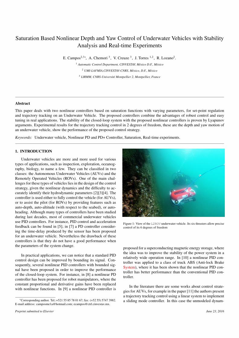
Saturation Based Nonlinear Depth and Yaw Control of Underwater Vehicles with StabilityAnalysis and Real-time Experiments
E. Campos2,3∗, A. Chemori 3 , V. Creuze 3 , J. Torres 1,2 , R. Lozano2.1 Automatic Control Department, CINVESTAV, Mexico D.F., Mexico
2 UMI-LAFMIA,CINVESTAV-CNRS, Mexico, D.F., Mexico
3 LIRMM, CNRS-Universite Montpellier 2, Montpellier, France
Abstract
This paper deals with two nonlinear controllers based on saturation functions with varying parameters, for set-point regulationand trajectory tracking on an Underwater Vehicle. The proposed controllers combine the advantages of robust control and easytuning in real applications. The stability of the closed-loop system with the proposed nonlinear controllers is proven by Lyapunovarguments. Experimental results for the trajectory tracking control in 2 degrees of freedom, these are the depth and yaw motion ofan underwater vehicle, show the performance of the proposed control strategy.
Keywords: Underwater vehicle, Nonlinear PD and PD+ Controller, Saturation, Real-time experiments.
1. INTRODUCTION
Underwater vehicles are more and more used for varioustypes of applications, such as inspection, exploration, oceanog-raphy, biology, to name a few. They can be classified in twoclasses: the Autonomous Underwater Vehicles (AUVs) and theRemotely Operated Vehicles (ROVs). One of the main chal-lenges for these types of vehicles lies in the design of the controlstrategy, given the nonlinear dynamics and the difficulty to ac-curately identify their hydrodynamic parameters [2][3][4]. Thecontroller is used either to fully control the vehicle (for AUVs),or to assist the pilot (for ROVs) by providing features such asauto-depth, auto-altitude (with respect to the seabed), or auto-heading. Although many types of controllers have been studiedduring last decades, most of commercial underwater vehiclesuse PID controllers. For instance, PID control and accelerationfeedback can be found in [5]; in [7] a PD controller consider-ing the time-delay produced by the sensor has been proposedfor an underwater vehicle. Nevertheless the drawback of thesecontrollers is that they do not have a good performance whenthe parameters of the system change.
In practical applications, we can notice that a standard PIDcontrol design can be improved by bounding its signal. Con-sequently, several nonlinear PID controllers with bounded sig-nal have been proposed in order to improve the performanceof the closed-loop system. For instance, in [8] a nonlinear PDcontroller has been proposed for robot manipulators, where theconstant proportional and derivative gains have been replacedwith nonlinear functions. In [9] a nonlinear PID controller is
∗Corresponding author. Tel.:+521 55 85 78 01 67; fax: (+52 55) 5747 3982.E-mail address: [email protected]; [email protected].
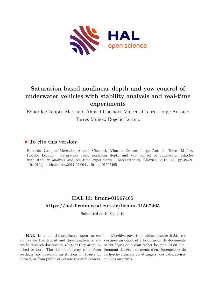
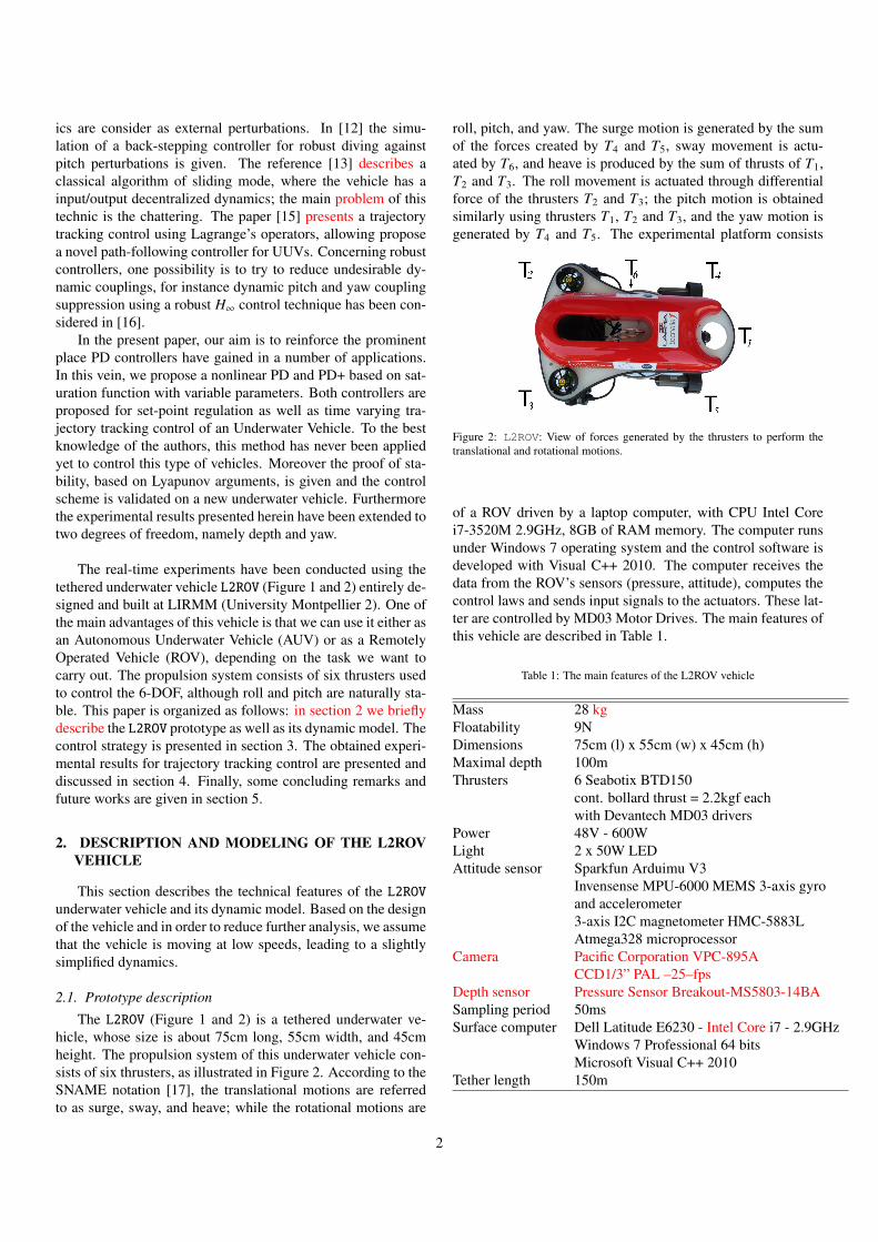
Figure 1: View of the L2ROV underwater vehicle. Its six thrusters allow precisecontrol of its 6 degrees of freedom
proposed for a superconducting magnetic energy storage, wherethe idea was to improve the stability of the power system in arelatively wide operation range. In [10] a nonlinear PID con-troller was applied to a class of truck ABS (Anti-lock BrakeSystem), where it has been shown that the nonlinear PID con-troller has better performance than the conventional PID con-troller.
In the literature there are some works about control strate-gies for AUVs, for example in the paper [11] the authors presenta trajectory tracking control using a linear system to implementa sliding mode controller. In this case the unmodeled dynam-
Preprint submitted to Elsevier June 23, 2016
ics are consider as external perturbations. In [12] the simu-lation of a back-stepping controller for robust diving againstpitch perturbations is given. The reference [13] describes aclassical algorithm of sliding mode, where the vehicle has ainput/output decentralized dynamics; the main problem of thistechnic is the chattering. The paper [15] presents a trajectorytracking control using Lagrange’s operators, allowing proposea novel path-following controller for UUVs. Concerning robustcontrollers, one possibility is to try to reduce undesirable dy-namic couplings, for instance dynamic pitch and yaw couplingsuppression using a robust H∞ control technique has been con-sidered in [16].
In the present paper, our aim is to reinforce the prominentplace PD controllers have gained in a number of applications.In this vein, we propose a nonlinear PD and PD+ based on sat-uration function with variable parameters. Both controllers areproposed for set-point regulation as well as time varying tra-jectory tracking control of an Underwater Vehicle. To the bestknowledge of the authors, this method has never been appliedyet to control this type of vehicles. Moreover the proof of sta-bility, based on Lyapunov arguments, is given and the controlscheme is validated on a new underwater vehicle. Furthermorethe experimental results presented herein have been extended totwo degrees of freedom, namely depth and yaw.
The real-time experiments have been conducted using thetethered underwater vehicle L2ROV (Figure 1 and 2) entirely de-signed and built at LIRMM (University Montpellier 2). One ofthe main advantages of this vehicle is that we can use it either asan Autonomous Underwater Vehicle (AUV) or as a RemotelyOperated Vehicle (ROV), depending on the task we want tocarry out. The propulsion system consists of six thrusters usedto control the 6-DOF, although roll and pitch are naturally sta-ble. This paper is organized as follows: in section 2 we brieflydescribe the L2ROV prototype as well as its dynamic model. Thecontrol strategy is presented in section 3. The obtained experi-mental results for trajectory tracking control are presented anddiscussed in section 4. Finally, some concluding remarks andfuture works are given in section 5.
2. DESCRIPTION AND MODELING OF THE L2ROVVEHICLE
This section describes the technical features of the L2ROVunderwater vehicle and its dynamic model. Based on the designof the vehicle and in order to reduce further analysis, we assumethat the vehicle is moving at low speeds, leading to a slightlysimplified dynamics.
2.1. Prototype description
The L2ROV (Figure 1 and 2) is a tethered underwater ve-hicle, whose size is about 75cm long, 55cm width, and 45cmheight. The propulsion system of this underwater vehicle con-sists of six thrusters, as illustrated in Figure 2. According to theSNAME notation [17], the translational motions are referredto as surge, sway, and heave; while the rotational motions are
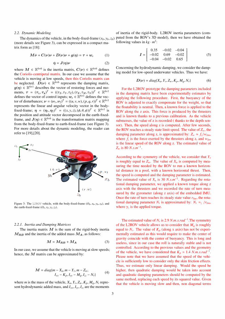
roll, pitch, and yaw. The surge motion is generated by the sumof the forces created by T4 and T5, sway movement is actu-ated by T6, and heave is produced by the sum of thrusts of T1,T2 and T3. The roll movement is actuated through differentialforce of the thrusters T2 and T3; the pitch motion is obtainedsimilarly using thrusters T1, T2 and T3, and the yaw motion isgenerated by T4 and T5. The experimental platform consists
Figure 2: L2ROV: View of forces generated by the thrusters to perform thetranslational and rotational motions.
of a ROV driven by a laptop computer, with CPU Intel Corei7-3520M 2.9GHz, 8GB of RAM memory. The computer runsunder Windows 7 operating system and the control software isdeveloped with Visual C++ 2010. The computer receives thedata from the ROV’s sensors (pressure, attitude), computes thecontrol laws and sends input signals to the actuators. These lat-ter are controlled by MD03 Motor Drives. The main features ofthis vehicle are described in Table 1.
Table 1: The main features of the L2ROV vehicle
Mass 28 kgFloatability 9NDimensions 75cm (l) x 55cm (w) x 45cm (h)Maximal depth 100mThrusters 6 Seabotix BTD150
cont. bollard thrust = 2.2kgf eachwith Devantech MD03 drivers
Power 48V - 600WLight 2 x 50W LEDAttitude sensor Sparkfun Arduimu V3
Invensense MPU-6000 MEMS 3-axis gyroand accelerometer3-axis I2C magnetometer HMC-5883LAtmega328 microprocessor
Camera Pacific Corporation VPC-895ACCD1/3” PAL –25–fps
Depth sensor Pressure Sensor Breakout-MS5803-14BASampling period 50msSurface computer Dell Latitude E6230 - Intel Core i7 - 2.9GHz
Windows 7 Professional 64 bitsMicrosoft Visual C++ 2010
Tether length 150m
2
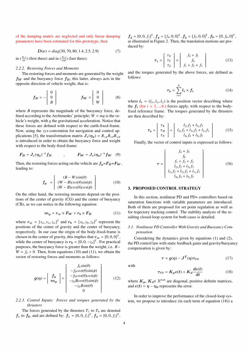
2.2. Dynamic ModelingThe dynamics of the vehicle, in the body-fixed-frame (xb, yb, zb)
(more details see Figure 3), can be expressed in a compact ma-trix form as [18]:
Mν +C(ν)ν +D(ν)ν + g(η) = τ +we (1)
η = J (η)ν (2)
where M ∈ R6×6 is the inertia matrix, C(ν) ∈ R6×6 definesthe Coriolis-centripetal matrix. In our case we assume that thevehicle is moving at low speeds, then this Coriolis matrix canbe neglected. D(ν) ∈ R6×6 represents the damping matrix,g(η) ∈ R6×1 describes the vector of restoring forces and mo-ments, τ = (τ, τ)T = ((τX , τY , τZ), (τK , τM , τN))T ∈ R6×1
defines the vector of control inputs; we ∈ R6×1 defines the vec-tor of disturbances; ν = (ν1,ν2)T = ((u, v,w), (p, q, r))T ∈ R6×1
represents the linear and angular velocity vector in the body-fixed-frame; η = (η1,η2)T = ((x, y, z), (φ, θ, ψ))T ∈ R6×1 isthe position and attitude vector decomposed in the earth-fixed-frame, and J (η) ∈ R6×6 is the transformation matrix mappingfrom the body-fixed-frame to earth-fixed-frame (see Figure 3).For more details about the dynamic modeling, the reader canrefer to [19],[20].
Figure 3: The L2ROV vehicle, with the body-fixed-frame (Ob, xb, yb, zb), andthe earth-fixed-frame (OI , xI , yI , zI ).
2.2.1. Inertia and Damping MatricesThe inertia matrix M is the sum of the rigid-body inertia
MRB and the inertia of the added massMA, as follows:
M =MRB +MA (3)
In our case, we assume that the vehicle is moving at slow speeds;hence, theM matrix can be approximated by:
M = diagm − Xu,m − Yv,m − Zw,Ixx − Kp, Iyy − Mq, Izz − Nr
(4)
where m is the mass of the vehicle, Xu,Yv,Zw,Kp,Mq,Nr repre-sent hydrodynamic added mass, and Ixx, Iyy, Izz are the moments
of inertia of the rigid-body. L2ROV inertia parameters (com-puted from the ROV’s 3D model), then we have obtained thefollowing values in kg · m2:
I =
0.35 −0.02 −0.04−0.02 0.69 −0.02−0.04 −0.02 0.65
(5)
Concerning the hydrodynamic damping, we consider the damp-ing model for low-speed underwater vehicles. Thus we have:
D(ν) = diagXu,Yv,Zw,Kp,Mq,Nr (6)
For the L2ROV prototype the damping parameters includedin the damping matrix have been experimentally estimates byapplying the following procedure. First, the buoyancy of theROV is adjusted to exactly compensate for the weight, so thatthe floatability is neutral. Then, a known force is applied to theROV along the z axis. This force is produced by the thrustersand is known thanks to a previous calibration. As the vehiclesubmerses, the value of z is recorded ( thanks to the depth sen-sor). Then, the speed along z is computed. After few seconds,the ROV reaches a steady state limit speed. The value of Zw, thedamping parameter along z, is approximated by: Zw ' fz/wlim,where fz is the force exerted by the thrusters along z, and wlim
is the linear speed of the ROV along z. The estimated value ofZw is 80 N.s.m−1.
According to the symmetry of the vehicle, we consider that Yv
is roughly equal to Zw. The value of Xu is computed by mea-suring the time needed by the ROV to run a known horizon-tal distance in a pool, with a known horizontal thrust. Then,the speed is computed and the damping parameter is estimated.The estimated value of Xu is 30 N.s.m−1. Regarding the rota-tional damping parameter, we applied a known torque along zaxis with the thrusters and we recorded the rate of turn mea-sured by the gyrometer (along z axis) of the embedded IMU.Once the rate of turn reaches its steady state value rlim, the rota-tional damping parameter Nr is approximated by: Nr 'z /rlim,where γz is the applied torque.
The estimated value of Nr is 2.9 N.m.s.rad−1.The symmetryof the L2ROV vehicle allows us to consider that Mq is roughlyequal to Nr. The value of Kp (along x axis) has not be experi-mentally estimated as this would require to make the center ofgravity coincide with the center of buoyancy. This is long anduseless, since in our case the roll is naturally stable and is notcontrolled. According to the previous values and the geometryof the vehicle, we have considered that Kp ' 1.4 N.m.s.rad−1.Please note that we have assumed that the speed of the vehi-cle is sufficiently low to consider only the skin friction effects.Thus, we estimate only linear damping. Would the speed behigher, then quadratic damping would be taken into accountand quadratic damping parameters should be computed by thesame method, replacing each speed by its squared value. Giventhat the vehicle is moving slow and then, non diagonal terms
3
of the damping matrix are neglected and only linear dampingparameters have been estimated for this prototype, then
D(ν) = diag30, 70, 80, 1.4, 2.5, 2.9 (7)
in ( N.sm ) (first three) and in ( N.s
rad ) (last three).
2.2.2. Restoring Forces and MomentsThe restoring forces and moments are generated by the weight
fW and the buoyancy force fB , this latter, always acts in theopposite direction of vehicle weight, that is:
fB = −
00B
fW =
00W
(8)
where B represents the magnitude of the buoyancy force, de-fined according to the Archimedes’ principle; W = mg is the ve-hicle’s weight, with g the gravitational acceleration. Notice thatthese forces are defined with respect to the earth-fixed-frame.Now, using the zyx-convention for navigation and control ap-plications [5], the transformation matrix J(η) = Rz,ψRy,θRx,φ
is introduced in order to obtain the buoyancy force and weightwith respect to the body-fixed-frame:
FB = J(η)−fB , FW = J(η)−fW (9)
Then, the restoring forces acting on the vehicle are fg=FB+FW ,leading to:
fg =
(B −W)sin(θ)(W − B)cos(θ)sin(φ)(W − B)cos(θ)cos(φ)
(10)
On the other hand, the restoring moments depend on the posi-tions of the center of gravity (CG) and the center of buoyancy(CB), as we can notice in the following equation:
mg = rw × FW + rb × FB (11)
where rw = [xw, yw, zw]T and rb = [xb, yb, zb]T represent thepositions of the center of gravity and the center of buoyancy,respectively. In our case the origin of the body-fixed-frame ischosen in the center of gravity, this implies that rw = [0, 0, 0]T ,while the center of buoyancy is rb = [0, 0,−zb]T . For practicalpurposes, the buoyancy force is greater than the weight, i.e. B−W = fb > 0. Then, from equations (10) and (11), we obtain thevector of restoring forces and moments as follows:
g(η) =[fgmg
]=
fbsin(θ)− fbcos(θ)sin(φ)− fbcos(θ)cos(φ)−zbBcos(θ)sin(φ)−zbBsin(θ)
0
(12)
2.2.3. Control Inputs: Forces and torques generated by thethrusters
The forces generated by the thrusters T1 to T6 are denotedf to f, and are defined by: f = [0, 0, f1]T , f = [0, 0, f2]T ,
f = [0, 0, f3]T , f = [ f4, 0, 0]T , f = [ f5, 0, 0]T , f = [0, f6, 0]T ,as illustrated in Figure 2. Then, the translation motions are pro-duced by:
τ =
τX
τY
τZ
= f4 + f5
f6f1 + f2 + f3
(13)
and the torques generated by the above forces, are defined asfollows:
τ =6∑
i=1
li × fi (14)
where li = (lix, liy, liz) is the position vector describing wherethe fi (for i = 1, .., 6.) forces apply, with respect to the body-fixed reference frame. The torques generated by the thrustersare then described by:
τ =
τK
τM
τN
= l2y f2 + l3y f3
l2x f2 + l3x f3 + l1x f1l4y f4 + l5y f5
(15)
Finally, the vector of control inputs is expressed as follows:
τ =
f4 + f5f6
f1 + f2 + f3l2y f2 + l3y f3
l2x f2 + l3x f3 + l1x f1l4y f4 + l5y f5
(16)
3. PROPOSED CONTROL STRATEGY
In this section, nonlinear PD and PD+ controllers based onsaturation functions with variable parameters are introduced.Both of them are proposed for set point regulation as well asfor trajectory tracking control. The stability analysis of the re-sulting closed-loop system for both cases is detailed.
3.1. Nonlinear PD Controller With Gravity and Buoyancy Com-pensation
Considering the dynamics given by equations (1) and (2),the PD control law with static feedback gains and gravity/buoyancycompensation is given by:
τ = g(η) − JT (η)τPD (17)
withτPD =Kpe(t) +Kd
de(t)dt
(18)
where Kp, Kd∈ R6×6 are diagonal, positive definite matrices,and e(t) = η − ηd represents the error.
In order to improve the performance of the closed-loop sys-tem, we propose to introduce (in each term of equation (18)) a
4
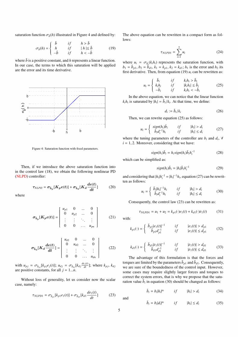
saturation function σb(h) illustrated in Figure 4 and defined by:
σb(h) =
b i f h > bh i f | h |≤ b−b i f h < −b
(19)
where b is a positive constant, and h represents a linear function.In our case, the terms to which this saturation will be appliedare the error and its time derivative.
Figure 4: Saturation function with fixed parameters.
Then, if we introduce the above saturation function intoin the control law (18), we obtain the following nonlinear PD(NLPD) controller:
τNLPD = σbp [Kpe(t)] + σbd [Kdde(t)dt
] (20)
where
σbp [Kpe(t)] =
up1 0 ... 00 up2 ... 0...
.... . .
...0 0 . . . upn
(21)
σbd [Kdde(t)dt
] =
ud1 0 ... 00 ud2 ... 0...
.... . .
...0 0 . . . udn
(22)
with up j = σbp j[kp je j(t)]; ud j = σbd j
[kd jde j(t)
dt ]; where kp j, kd j
are positive constants, for all j = 1...n.
Without loss of generality, let us consider now the scalarcase, namely:
τNLPD1 = σbp1[kp1e1(t)] + σbd1
[kd1de1(t)
dt] (23)
The above equation can be rewritten in a compact form as fol-lows:
τNLPD1 =
2∑i=1
ui (24)
where ui = σbi(kihi) represents the saturation function, with
b1 = bp1, b2 = bd1, k1 = kp1, k2 = kd1; h1 is the error and h2 itsfirst derivative. Then, from equation (19) ui can be rewritten as:
ui =
bi i f kihi > bi
kihi i f |kihi| ≤ bi
−bi i f kihi < −bi
(25)
In the above equation, we can notice that the linear functionkihi is saturated by |hi| = bi/ki. At that time, we define:
di := bi/ki (26)
Then, we can rewrite equation (25) as follows:
ui =
sign(hi)bi i f |hi| > di
bid−1i hi i f |hi| ≤ di
(27)
where the tuning parameters of the controller are bi and di, ∀i = 1, 2. Moreover, considering that we have:
sign(hi)bi = hisign(hi)bih−1i (28)
which can be simplified as:
sign(hi)bi = |hi|bih−1i (29)
and considering that |hi|h−1i = |hi|
−1hi, equation (27) can be rewrit-ten as follows:
ui =
bi|hi|
−1hi i f |hi| > di
bid−1i hi i f |hi| ≤ di
(30)
Consequently, the control law (23) can be rewritten as:
τNLPD1 = u1 + u2 = kp1(·)e1(t) + kd1(·)e1(t) (31)
with:
kp1(·) =
bp1|e1(t)|−1 i f |e1(t)| > dp1bp1d−1
p1 i f |e1(t)| ≤ dp1(32)
kd1(·) =
bd1|e1(t)|−1 i f |e1(t)| > dd1bd1d−1
d1 i f |e1(t)| ≤ dd1(33)
The advantage of this formulation is that the forces andtorques are limited by the parameters bp1 and bd1. Consequently,we are sure of the boundedness of the control input. However,some cases may require slightly larger forces and torques tocorrect the system errors, that is why we propose that the satu-ration value bi in equation (30) should be changed as follows:
bi = bi|hi|µi i f |hi| > di (34)
andbi = bi|di|
µi i f |hi| ≤ di (35)
5
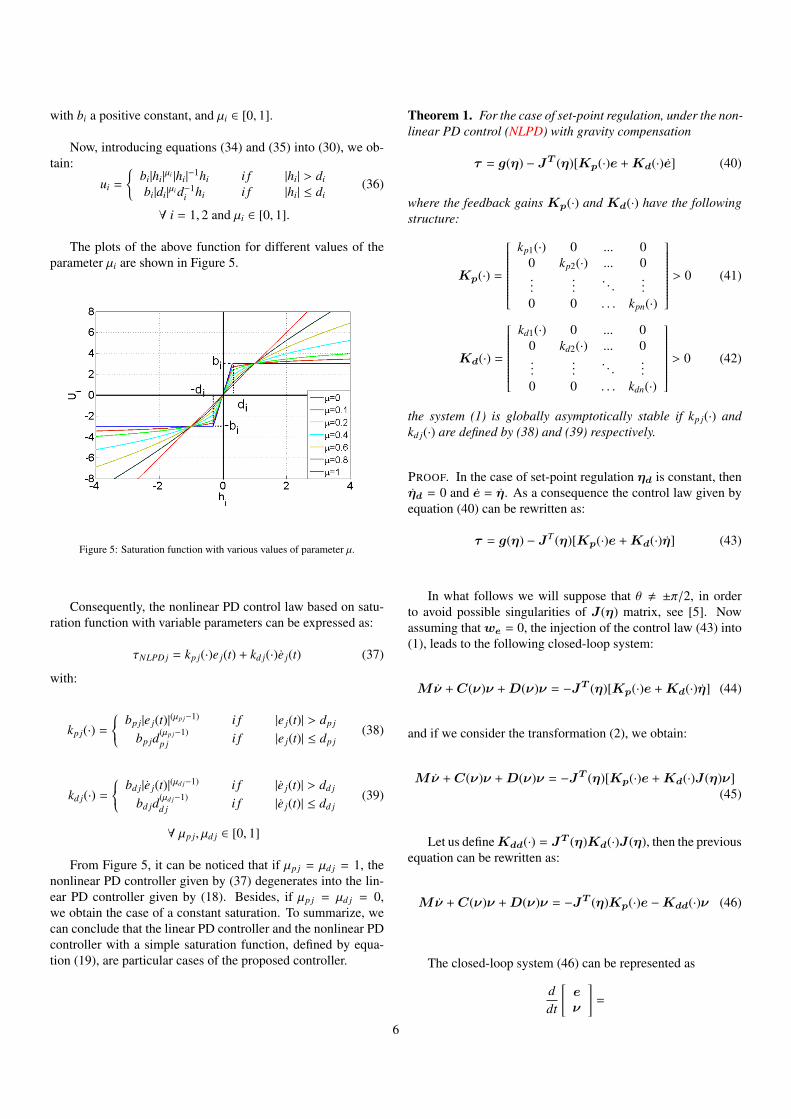
with bi a positive constant, and µi ∈ [0, 1].
Now, introducing equations (34) and (35) into (30), we ob-tain:
ui =
bi|hi|
µi |hi|−1hi i f |hi| > di
bi|di|µi d−1
i hi i f |hi| ≤ di(36)
∀ i = 1, 2 and µi ∈ [0, 1].
The plots of the above function for different values of theparameter µi are shown in Figure 5.
Figure 5: Saturation function with various values of parameter µ.
Consequently, the nonlinear PD control law based on satu-ration function with variable parameters can be expressed as:
τNLPD j = kp j(·)e j(t) + kd j(·)e j(t) (37)
with:
kp j(·) = bp j|e j(t)|(µp j−1) i f |e j(t)| > dp j
bp jd(µp j−1)p j i f |e j(t)| ≤ dp j
(38)
kd j(·) = bd j|e j(t)|(µd j−1) i f |e j(t)| > dd j
bd jd(µd j−1)d j i f |e j(t)| ≤ dd j
(39)
∀ µp j, µd j ∈ [0, 1]
From Figure 5, it can be noticed that if µp j = µd j = 1, thenonlinear PD controller given by (37) degenerates into the lin-ear PD controller given by (18). Besides, if µp j = µd j = 0,we obtain the case of a constant saturation. To summarize, wecan conclude that the linear PD controller and the nonlinear PDcontroller with a simple saturation function, defined by equa-tion (19), are particular cases of the proposed controller.
Theorem 1. For the case of set-point regulation, under the non-linear PD control (NLPD) with gravity compensation
τ = g(η) − JT (η)[Kp(·)e +Kd(·)e] (40)
where the feedback gains Kp(·) and Kd(·) have the followingstructure:
Kp(·) =
kp1(·) 0 ... 0
0 kp2(·) ... 0...
.... . .
...0 0 . . . kpn(·)
> 0 (41)
Kd(·) =
kd1(·) 0 ... 0
0 kd2(·) ... 0...
.... . .
...0 0 . . . kdn(·)
> 0 (42)
the system (1) is globally asymptotically stable if kp j(·) andkd j(·) are defined by (38) and (39) respectively.
PROOF. In the case of set-point regulation ηd is constant, thenηd = 0 and e = η. As a consequence the control law given byequation (40) can be rewritten as:
τ = g(η) − JT (η)[Kp(·)e +Kd(·)η] (43)
In what follows we will suppose that θ , ±π/2, in orderto avoid possible singularities of J (η) matrix, see [5]. Nowassuming thatwe = 0, the injection of the control law (43) into(1), leads to the following closed-loop system:
Mν +C(ν)ν +D(ν)ν = −JT (η)[Kp(·)e +Kd(·)η] (44)
and if we consider the transformation (2), we obtain:
Mν +C(ν)ν +D(ν)ν = −JT (η)[Kp(·)e +Kd(·)J (η)ν](45)
Let us defineKdd(·) = JT (η)Kd(·)J (η), then the previousequation can be rewritten as:
Mν +C(ν)ν +D(ν)ν = −JT (η)Kp(·)e −Kdd(·)ν (46)
The closed-loop system (46) can be represented as
ddt
[eν
]=
6
[J (η)ν
M−[−JT (η)Kp(·)e −Kdd(·)ν −C(ν)ν −D(ν)ν]
](47)
Notice that the origin of the state space model is a unique equi-librium point. Now, in order to proof the globally asymptoticstability of the closed-loop system we propose the followingLyapunov function candidate:
V(e,ν) =12νTMν +
∫ e
ξTKp(ξ)dξ (48)
where∫ eξTKp(ξ)dξ =
∫ e1
0 ξ1kp1(ξ1)dξ1 +∫ e2
0 ξ2kp2(ξ2)dξ2+∫ e3
0 ξ3kp3(ξ3)dξ3 + ... +∫ en
0 ξnkpn(ξn)dξn.
Now, considering that the inequality
e jkp j(·) ≥ α j(|e j|) (49)
is satisfied with the classK functions
α j(|e j|) =
b j |e j |
µp j e j
a+|e j |i f |e j| > d j
b jdµp jj e j
a+d ji f |e j| ≤ d j
(50)
with bp j > b j, a > 0 and dp j < d j. Then, according to Lemma 2from [8] one deduces the following:∫ e
ξTKp(ξ)dξ >0 ∀ e , 0 ∈ Rn (51)
and ∫ e
ξTKp(ξ)dξ → ∞ as ‖ e ‖→ ∞ (52)
Therefore, the Lyapunov function candidate V(e,ν) is aglobally positive definite and radially unbounded.
The time derivative of the Lyapunov function candidate is:
V(e,ν) = νTMν + eTKp(e)J (η)ν (53)
by substituting the closed-loop equation (46) into (53) one ob-tains:
V(e,ν) = −νTJT (η)Kp(e)e − νTKdd(η, e)ν−νTC(ν)ν − νTD(ν)ν + eTKp(e)J (η)ν (54)
sinceKp(e) =KTp (e) andC(ν) = −C(ν)T , equation (54) be-
comes:
V(e,ν) = −νT [Kdd(η, e) +D(ν)]ν (55)
Recall thatKd =KTd > 0, thereforeKdd =K
Tdd > 0, and
assuming that D(ν) > 0, then one can conclude that V(e,ν) isa globally negative semidefinite. Therefore the stability of theequilibrium point is guaranteed. In order to prove the asymp-totic stability, the Krasovskii-LaSalle’s theorem can be used, let
Ω =
[eν
]: V(e,ν) = 0
=
[eν
]=
[e0
]∈ R2n
(56)
introducing ν =0 and ν =0 into equation (46) leads to the uniqueinvariant point e =0. Therefore, we conclude that equilibriumpoint is globally asymptotically stable.
3.2. Nonlinear PD+ Controller
For the case of trajectory tracking problem, we propose touse a nonlinear PD+ controller with the same feedback gains asthe previous controller.
Based on equation (2), the following kinematic transforma-tions can be obtained (see [5] for more details):
η = J (η)ν + J (η)ν =⇒ ν = J−(η)[η − J (η)J−(η)η]
Applying the previous transformations to the dynamic model(1), one obtains:
Mη(η) = J−T (η)MJ−(η)Cη(ν,η) = J−T (η)[C(ν) −MJ−(η)J (η)]J−(η)Dη(ν,η) = J−T (η)D(ν)J−(η)gη(η) = J−T (η)g(η)τη(η) = J−T (η)τ
Consequently, the dynamic model (1) expressed in the earth-fixed-frame becomes:
Mη(η)η +Cη(ν,η)η +Dη(ν,η)η + gη(η) = J−T (η)τ(57)
Theorem 2. For the case of the trajectory tracking control, thenonlinear PD+ controller (NLPD+):
τ = −JT (η)[Mη(η)ηd +Cη(ν,η)ηd +Dη(ν,η)ηd+gη(η) +Kp(·)e +Kd(·)e]
(58)where the matrices Kp(·) and Kd(·) have the following struc-ture:
Kp(·) =
kp1(·) 0 ... 0
0 kp2(·) ... 0...
.... . .
...0 0 . . . kpn(·)
> 0 (59)
7
Kd(·) =
kd1(·) 0 ... 0
0 kd2(·) ... 0...
.... . .
...0 0 . . . kdn(·)
> 0 (60)
globally asymptotically stabilizes the system (1) if kp j(·) andkd j(·) are defined by (38) and (39) respectively.
PROOF. Injecting the control law (58) in equation (57), leadsto the following closed-loop system:
Mη(η)e = −Cη(ν,η)e −Dη(ν,η)e −Kp(·)e −Kd(·)e(61)
which can be rewritten as:
ddt
[ee
]=
[e
−Mη(η)−[[Cη(ν,η) +Dη(ν,η) +Kd(·)]e +Kp(·)e]
](62)
where it can be noticed that the resulting system is autonomousand the origin is its unique equilibrium point.
The stability analysis can be conducted in the same wayas for the previous controller, then considering the followingLyapunov function candidate:
V(e, e) =12eTMη(η)e +
∫ e
ξTKp(ξ)dξ (63)
and according to arguments used in proof of the previous sec-tion, we conclude that V(e, e) is also globally positive definiteand radially unbounded.
The time derivative of this Lyapunov function candidategives:
V(e, e) = eTMη(η)e +12eT Mη(η)e + eTKp(·)e (64)
Now, injecting equation (61) in (64) and assuming that Mη =0,and Cη(ν,η) is skew symmetric, then:
V(e, e) = −eT [Dη(ν,η) +Kd(·)]e (65)
Assuming that Dη(ν,η) > 0 and remembering that Kd(·) > 0and symmetric matrix, we deduce that V(e, e) is globally neg-ative semidefinite, and therefore we can conclude stability ofthe equilibrium point. In order to prove asymptotic stability weapply the Krasovskii-LaSalle’s theorem. Consider the set Ωdefined as:
Ω =
[ee
]: V(e, e) = 0
=
[ee
]=
[e0
]∈ R2n
(66)
Introducing e =0 and e =0 into equation (61), we deduce thatthe unique invariant set is defined by e =0. As a consequencewe conclude that equilibrium point is globally asymptoticallystable. Notices that in case of ηd constant, the nonlinear PD+controller degenerates to the nonlinear PD controller presentedin the previous section.
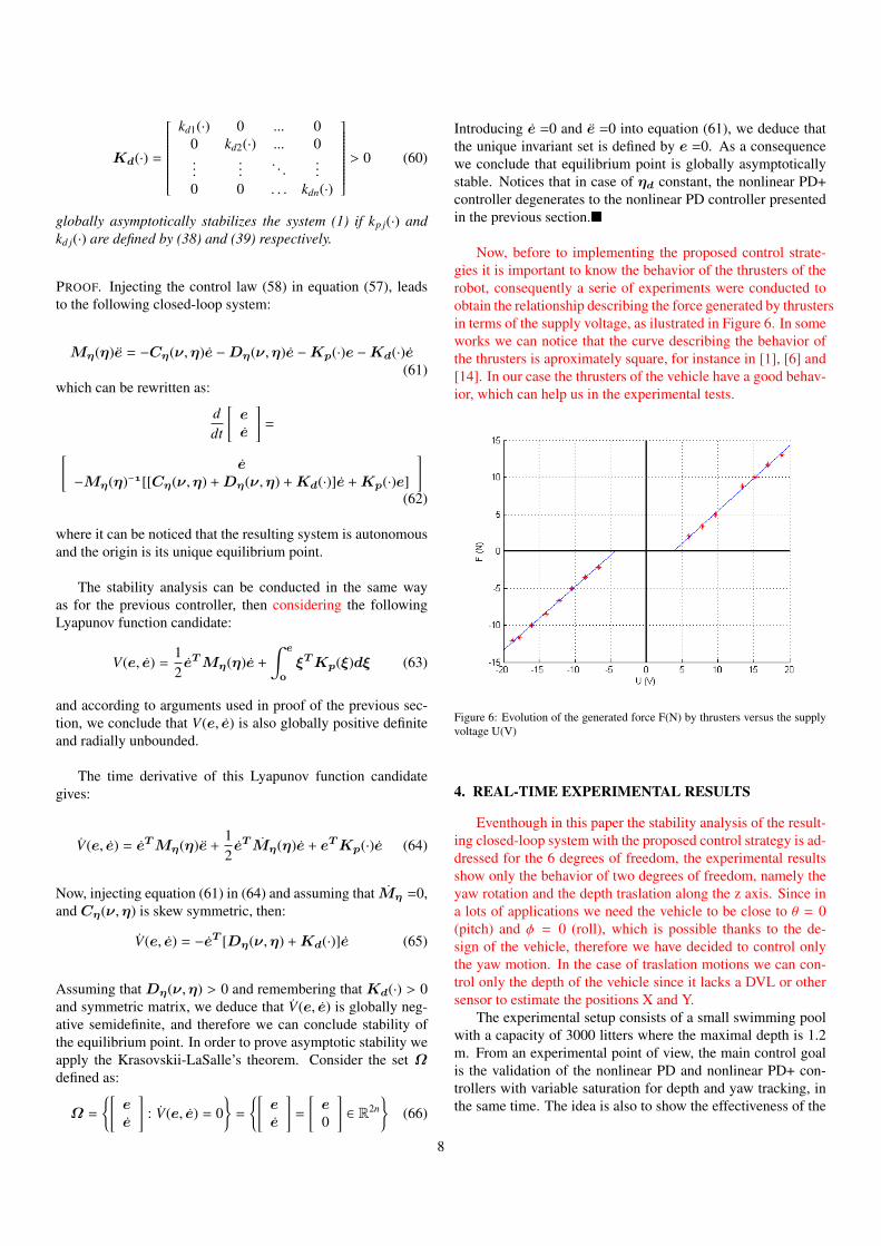
Now, before to implementing the proposed control strate-gies it is important to know the behavior of the thrusters of therobot, consequently a serie of experiments were conducted toobtain the relationship describing the force generated by thrustersin terms of the supply voltage, as ilustrated in Figure 6. In someworks we can notice that the curve describing the behavior ofthe thrusters is aproximately square, for instance in [1], [6] and[14]. In our case the thrusters of the vehicle have a good behav-ior, which can help us in the experimental tests.
Figure 6: Evolution of the generated force F(N) by thrusters versus the supplyvoltage U(V)
4. REAL-TIME EXPERIMENTAL RESULTS
Eventhough in this paper the stability analysis of the result-ing closed-loop system with the proposed control strategy is ad-dressed for the 6 degrees of freedom, the experimental resultsshow only the behavior of two degrees of freedom, namely theyaw rotation and the depth traslation along the z axis. Since ina lots of applications we need the vehicle to be close to θ = 0(pitch) and φ = 0 (roll), which is possible thanks to the de-sign of the vehicle, therefore we have decided to control onlythe yaw motion. In the case of traslation motions we can con-trol only the depth of the vehicle since it lacks a DVL or othersensor to estimate the positions X and Y.
The experimental setup consists of a small swimming poolwith a capacity of 3000 litters where the maximal depth is 1.2m. From an experimental point of view, the main control goalis the validation of the nonlinear PD and nonlinear PD+ con-trollers with variable saturation for depth and yaw tracking, inthe same time. The idea is also to show the effectiveness of the
8
proposed control solution against possible changes in the buoy-ancy and damping parameters that may occur during the exper-iments. The experimental results proposed hereafter have beenconducted through the implementation of the proposed con-trollers on the of L2ROV underwater vehicle, you can watch thereal-time experiments in: www.youtube.com/watch?v=SZZm4He2-CA&feature=youtu.be.
4.1. Proposed experimental scenarios
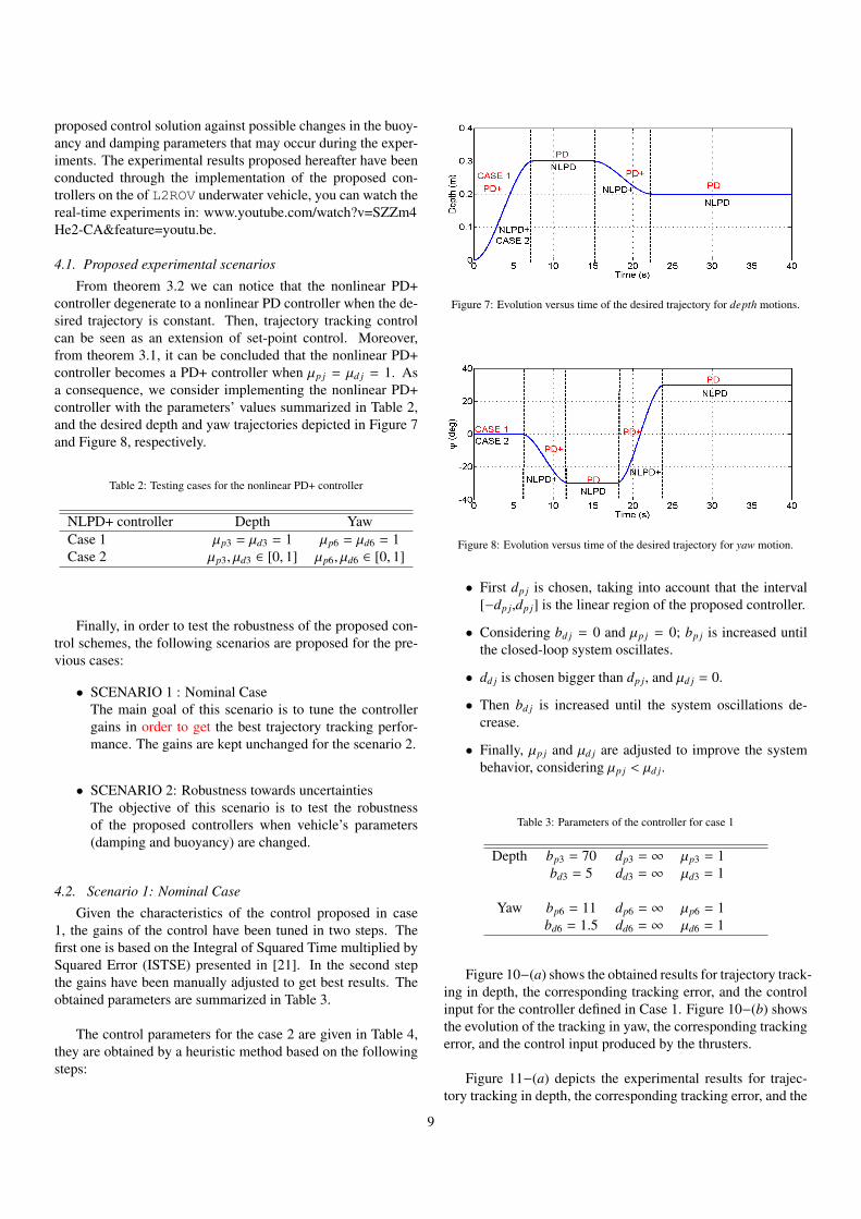
From theorem 3.2 we can notice that the nonlinear PD+controller degenerate to a nonlinear PD controller when the de-sired trajectory is constant. Then, trajectory tracking controlcan be seen as an extension of set-point control. Moreover,from theorem 3.1, it can be concluded that the nonlinear PD+controller becomes a PD+ controller when µp j = µd j = 1. Asa consequence, we consider implementing the nonlinear PD+controller with the parameters’ values summarized in Table 2,and the desired depth and yaw trajectories depicted in Figure 7and Figure 8, respectively.
Table 2: Testing cases for the nonlinear PD+ controller
NLPD+ controller Depth YawCase 1 µp3 = µd3 = 1 µp6 = µd6 = 1Case 2 µp3, µd3 ∈ [0, 1] µp6, µd6 ∈ [0, 1]
Finally, in order to test the robustness of the proposed con-trol schemes, the following scenarios are proposed for the pre-vious cases:
• SCENARIO 1 : Nominal CaseThe main goal of this scenario is to tune the controllergains in order to get the best trajectory tracking perfor-mance. The gains are kept unchanged for the scenario 2.
• SCENARIO 2: Robustness towards uncertaintiesThe objective of this scenario is to test the robustnessof the proposed controllers when vehicle’s parameters(damping and buoyancy) are changed.
4.2. Scenario 1: Nominal Case
Given the characteristics of the control proposed in case1, the gains of the control have been tuned in two steps. Thefirst one is based on the Integral of Squared Time multiplied bySquared Error (ISTSE) presented in [21]. In the second stepthe gains have been manually adjusted to get best results. Theobtained parameters are summarized in Table 3.
The control parameters for the case 2 are given in Table 4,they are obtained by a heuristic method based on the followingsteps:
Figure 7: Evolution versus time of the desired trajectory for depth motions.
Figure 8: Evolution versus time of the desired trajectory for yaw motion.
• First dp j is chosen, taking into account that the interval[−dp j,dp j] is the linear region of the proposed controller.
• Considering bd j = 0 and µp j = 0; bp j is increased untilthe closed-loop system oscillates.
• dd j is chosen bigger than dp j, and µd j = 0.
• Then bd j is increased until the system oscillations de-crease.
• Finally, µp j and µd j are adjusted to improve the systembehavior, considering µp j < µd j.
Table 3: Parameters of the controller for case 1
Depth bp3 = 70 dp3 = ∞ µp3 = 1bd3 = 5 dd3 = ∞ µd3 = 1
Yaw bp6 = 11 dp6 = ∞ µp6 = 1bd6 = 1.5 dd6 = ∞ µd6 = 1
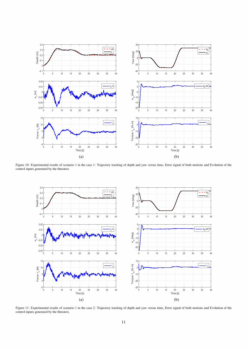
Figure 10−(a) shows the obtained results for trajectory track-ing in depth, the corresponding tracking error, and the controlinput for the controller defined in Case 1. Figure 10−(b) showsthe evolution of the tracking in yaw, the corresponding trackingerror, and the control input produced by the thrusters.
Figure 11−(a) depicts the experimental results for trajec-tory tracking in depth, the corresponding tracking error, and the
9
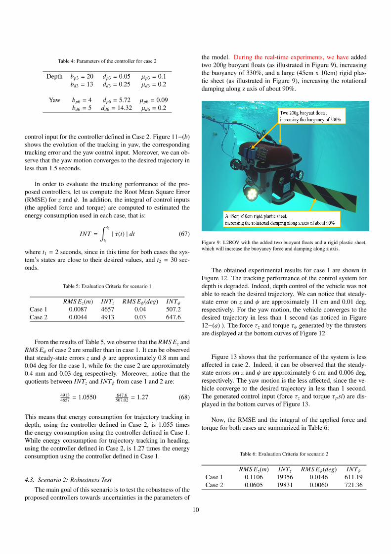
Table 4: Parameters of the controller for case 2
Depth bp3 = 20 dp3 = 0.05 µp3 = 0.1bd3 = 13 dd3 = 0.25 µd3 = 0.2
Yaw bp6 = 4 dp6 = 5.72 µp6 = 0.09bd6 = 5 dd6 = 14.32 µd6 = 0.2
control input for the controller defined in Case 2. Figure 11−(b)shows the evolution of the tracking in yaw, the correspondingtracking error and the yaw control input. Moreover, we can ob-serve that the yaw motion converges to the desired trajectory inless than 1.5 seconds.
In order to evaluate the tracking performance of the pro-posed controllers, let us compute the Root Mean Square Error(RMSE) for z and ψ. In addition, the integral of control inputs(the applied force and torque) are computed to estimated theenergy consumption used in each case, that is:
INT =∫ t2
t1| τ(t) | dt (67)
where t1 = 2 seconds, since in this time for both cases the sys-tem’s states are close to their desired values, and t2 = 30 sec-onds.
Table 5: Evaluation Criteria for scenario 1
RMS Ez(m) INTz RMS Eψ(deg) INTψCase 1 0.0087 4657 0.04 507.2Case 2 0.0044 4913 0.03 647.6
From the results of Table 5, we observe that the RMS Ez andRMS Eψ of case 2 are smaller than in case 1. It can be observedthat steady-state errors z and ψ are approximately 0.8 mm and0.04 deg for the case 1, while for the case 2 are approximately0.4 mm and 0.03 deg respectively. Moreover, notice that thequotients between INTz and INTψ from case 1 and 2 are:
49134657 = 1.0550 647.6
507.02 = 1.27 (68)
This means that energy consumption for trajectory tracking indepth, using the controller defined in Case 2, is 1.055 timesthe energy consumption using the controller defined in Case 1.While energy consumption for trajectory tracking in heading,using the controller defined in Case 2, is 1.27 times the energyconsumption using the controller defined in Case 1.
4.3. Scenario 2: Robustness Test
The main goal of this scenario is to test the robustness of theproposed controllers towards uncertainties in the parameters of
the model. During the real-time experiments, we have addedtwo 200g buoyant floats (as illustrated in Figure 9), increasingthe buoyancy of 330%, and a large (45cm x 10cm) rigid plas-tic sheet (as illustrated in Figure 9), increasing the rotationaldamping along z axis of about 90%.
Figure 9: L2ROV with the added two buoyant floats and a rigid plastic sheet,which will increase the buoyancy force and damping along z axis.
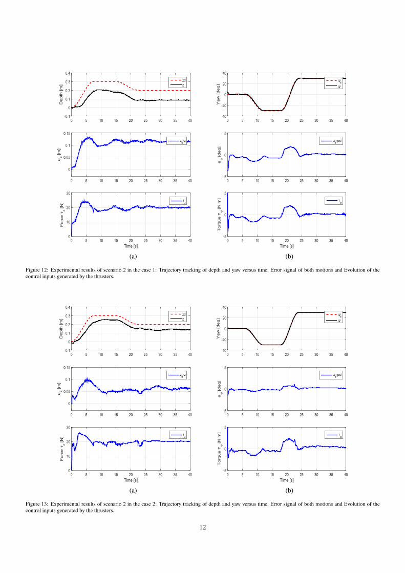
The obtained experimental results for case 1 are shown inFigure 12. The tracking performance of the control system fordepth is degraded. Indeed, depth control of the vehicle was notable to reach the desired trajectory. We can notice that steady-state error on z and ψ are approximately 11 cm and 0.01 deg,respectively. For the yaw motion, the vehicle converges to thedesired trajectory in less than 1 second (as noticed in Figure12−(a) ). The force τz and torque τψ generated by the thrustersare displayed at the bottom curves of Figure 12.
Figure 13 shows that the performance of the system is lessaffected in case 2. Indeed, it can be observed that the steady-state errors on z and ψ are approximately 6 cm and 0.006 deg,respectively. The yaw motion is the less affected, since the ve-hicle converge to the desired trajectory in less than 1 second.The generated control input (force τz and torque τpsi) are dis-played in the bottom curves of Figure 13.
Now, the RMSE and the integral of the applied force andtorque for both cases are summarized in Table 6:
Table 6: Evaluation Criteria for scenario 2
RMS Ez(m) INTz RMS Eψ(deg) INTψCase 1 0.1106 19356 0.0146 611.19Case 2 0.0605 19831 0.0060 721.36
10
0 5 10 15 20 25 30 35 40
De
pth
[m
]
-0.1
0
0.1
0.2
0.3
0.4
zdz
0 5 10 15 20 25 30 35 40
ez
[m]
-0.03
-0.02
-0.01
0
0.01
0.02
zd-z
Time [s]0 5 10 15 20 25 30 35 40
Fo
rceτ z
[N]
-5
0
5
10
15
τz
0 5 10 15 20 25 30 35 40
Ya
w [
de
g]
-40
-20
0
20
40
ψd
ψ
0 5 10 15 20 25 30 35 40
eψ
[de
g]
-20
-15
-10
-5
0
5
ψd-psi
Time [s]0 5 10 15 20 25 30 35 40
To
rqu
e τψ
[N.m
]
-30
-20
-10
0
10
τψ
(a) (b)
Figure 10: Experimental results of scenario 1 in the case 1: Trajectory tracking of depth and yaw versus time, Error signal of both motions and Evolution of thecontrol inputs generated by the thrusters.
0 5 10 15 20 25 30 35 40
De
pth
[m
]
-0.1
0
0.1
0.2
0.3
0.4
zdz
0 5 10 15 20 25 30 35 40
ez
[m]
-0.03
-0.02
-0.01
0
0.01
0.02
zd-z
Time [s]0 5 10 15 20 25 30 35 40
Fo
rceτ z
[N]
-5
0
5
10
15
τz
0 5 10 15 20 25 30 35 40
Ya
w [
de
g]
-40
-20
0
20
40
ψd
ψ
0 5 10 15 20 25 30 35 40
eψ
[de
g]
-20
-15
-10
-5
0
5
ψd-psi
Time [s]0 5 10 15 20 25 30 35 40
To
rqu
e τψ
[N.m
]
-30
-20
-10
0
10
τψ
(a) (b)
Figure 11: Experimental results of scenario 1 in the case 2: Trajectory tracking of depth and yaw versus time, Error signal of both motions and Evolution of thecontrol inputs generated by the thrusters.
11
0 5 10 15 20 25 30 35 40
De
pth
[m
]
-0.1
0
0.1
0.2
0.3
0.4
zdz
0 5 10 15 20 25 30 35 40
ez
[m]
0
0.05
0.1
0.15
zd-z
Time [s]0 5 10 15 20 25 30 35 40
Fo
rceτ z
[N]
0
10
20
30
τz
0 5 10 15 20 25 30 35 40
Ya
w [
de
g]
-40
-20
0
20
40
ψd
ψ
0 5 10 15 20 25 30 35 40
eψ
[de
g]
-5
0
5
ψd-psi
Time [s]0 5 10 15 20 25 30 35 40
To
rqu
e τψ
[N.m
]
-5
0
5
τψ
(a) (b)
Figure 12: Experimental results of scenario 2 in the case 1: Trajectory tracking of depth and yaw versus time, Error signal of both motions and Evolution of thecontrol inputs generated by the thrusters.
0 5 10 15 20 25 30 35 40
De
pth
[m
]
-0.1
0
0.1
0.2
0.3
0.4
zdz
0 5 10 15 20 25 30 35 40
ez
[m]
0
0.05
0.1
0.15
zd-z
Time [s]0 5 10 15 20 25 30 35 40
Fo
rceτ z
[N]
0
10
20
30
τz
0 5 10 15 20 25 30 35 40
Ya
w [
de
g]
-40
-20
0
20
40
ψd
ψ
0 5 10 15 20 25 30 35 40
eψ
[de
g]
-5
0
5
ψd-psi
Time [s]0 5 10 15 20 25 30 35 40
To
rqu
e τψ
[N.m
]
-5
0
5
τψ
(a) (b)
Figure 13: Experimental results of scenario 2 in the case 2: Trajectory tracking of depth and yaw versus time, Error signal of both motions and Evolution of thecontrol inputs generated by the thrusters.
12
According to Table 6 the quotients between INTz and INTψfrom case 1 and 2 are:
1983119356 = 1.0245 721.36
611.19 = 1.1803 (69)
This means that energy consumption for trajectory trackingin depth, using the controller defined in Case 2, is 1.05 timesthe energy consumption using the controller define in Case 1.While energy consumption for trajectory tracking in heading,using the controller defined in Case 2, is 1.27 times the energyconsumption using the controller defined in Case 1. We can ob-serve that the quotients obtained in this scenario are very similaras in the previous scenario, see equation (68). Moreover, onecan notice that the closed-loop system with the nonlinear PD+controller, represented by case 2, is less affected. It can be ob-served that steady-state errors z and ψ are approximately 11 cmand 0.01 deg for the case 1, while for the case 2 their valuesare approximately 6 cm and 0.006 deg respectively. Moreover,notice that the chattering is large in the second case than inthe first one. This is due to the stronger compromise betweenperformance and robustness imposed by the variable saturationcase. Then, we can conclude that the proposed control strategydemonstrated a good ability to deal with parameters’ uncertain-ties.
5. CONCLUSION AND FUTURE WORK
In this paper, a nonlinear PD and PD+ controllers have beenproposed for depth and yaw control of underwater vehicles. Thestability analysis for the resulting closed-loop system for bothset-point regulation and trajectory tracking control has been ad-dressed. The proposed controllers have been implemented fortrajectory tracking in depth and yaw motions with the L2ROVunderwater vehicle. The obtained experimental results demon-strate the effectiveness and the robustness of the proposed con-trollers towards uncertainties on the parameters of the system(damping and buoyancy changes). The future work will consistin implementing the integral term of the controller in order toimprove the steady-state performance of the closed-loop sys-tem.
6. ACKNOWLEDGEMENTS
This work was supported by the PCP research project, incollaboration with the Tecnalia foundation. The L2ROV un-derwater vehicle has been funded by the Region Languedoc-Roussillon council (ARPE MiniROV). The authors greatly ac-knowledge support of the European Union through FEDER grantn 49793 for the development of the Leonard L2ROV
References
[1] Allotta B., Pugi L., Bartolini F., Ridolfi A., Costanzi R., Monni N.,Gelli J., Preliminary design and fast prototyping of an Autonomous Un-derwater Vehicle propulsion system, Proceedings of the Institution of Me-chanical Engineers Part M: Journal of Engineering for the Maritime En-vironment, 229 (3), pp. 248-272, 2015.
[2] Newman. Marine Hydrodynamics MIT Press. Cambridge, MA. J.N.1977.
[3] Thor I. Fossen. Handbook of Marine Craft Hydrodynamics and MotionControl. John Wiley, 2011.
[4] H. Lamb. (1932).Hydrodynamics. Cambridge University Press. London[5] Thor I. Fossen. Marine control systems guidance, navigation, and control
of shipd, rigs and underwater vehicles. Marine Cybernetics, 2002.[6] Carlton J., Marine Propellers and Propulsion, 2nd edition, Elsevier, 2007.[7] E. Campos, I. Torres, O. Garcia., J. Torres and R. Lozano. Embedded
system for controlling a mini underwater vehicle in autonomous hovermode CESCIT 2012, Germany, April 3-5.
[8] R. Kelly, Ricardo c. A class of nonlinear PD-type controller for robotmanupulator. J Robotic Syst, 1996;13:793-802.
[9] X.Peng, Shijie Cheng, and Jinyu Wen. Application of Nonlinear PIDController in Superconducting Magnetic Energy Storage InternationalJournal of Control, Automation, and Systems, vol. 3, no. 2, pp. 296-301,June 2005.
[10] F. Jiang Zhiqiang Gao. An Application of Nonlinear PID Control to aClass of Truck ABS Problems Decision and Control 2001, Vol.1. Pro-ceedings of the 40th IEEE Conference.
[11] David Bryan Marco and Anthony J. Healey Command, Control, and Nav-igation Experimental Results With the NPS ARIES AUV. IEEE Journal ofOceanic Engineerin, Vol. 26, No. 4, October 2001.
[12] Lionel Lapierre Robust diving control of an AUV. Ocean Engineering,36 (2009), 92-104.
[13] Petko Kiriazov, Edwin Kreuzer, Fernando C. Pinto Robust feedback sta-bilization of underwater robotic vehicles. Robotics and Autonomous Sys-tems 21 (1997) 415-423.
[14] Pivano L., Johansen T. A., Smogeli, N., A Four-Quadrant Thrust Esti-mation Scheme for Marine Propellers: Theory and Experiments, IEEETrans. on Control Systems Technology, 17 (1), 2009.
[15] Ehsan Peymani, Thor I. Fossen Path following of underwater robots usingLagrange multipliers. Robotics and Autonomous Systems 2014.
[16] Petirch, J. and Stilwell D.J. Robust control for an autonomous vehiclethat suppresses pitch and yaw couplings. Ocean Engineering, 38 (2011),197-204.
[17] The Society of Naval Architects and Marine Engineers. Nomenclature forTreating the Motion of a Submerged Body Through a Fluid. IN: Technicaland Research Bulletin No. 1-5.
[18] Thor I. Fossen. Guidance and Control of Ocean Vehicles. John Wiley andSons, Norway, Secondedition, 1999.
[19] H. Goldstein, C.P. Poole and J.L Safko. Classical Mechanics. AddisonWesley Series in Physics,Adison-Wesley, USA, second edition, 1983.
[20] J.E. Marsden. Elementary Classical Analysis. W.H. Freeman and Com-pany, San Francisco, 1974.
[21] A Visioli. Optimal tuning of pid controllers for integral and unstableprocesses. Proceedings of the IEEE, Part D, 148(2):180-194, 2001.
13