Saturation of curvature-induced secondary flow, energy ... · and turbulence in sharp open-channel bends: Laboratory ... and bathymetric characteristics in meander bends [van

Saturation of curvature-induced secondary flow, energy losses,

and turbulence in sharp open-channel bends: Laboratory

experiments, analysis, and modeling

K. Blanckaert1,2

Received 14 August 2008; revised 24 April 2009; accepted 4 June 2009; published 27 August 2009.

[1] The paper investigates the influence of relative bend curvature on secondary flow,energy losses, and turbulence in sharp open-channel bends. These processes are importantin natural streams with respect to sediment transport, the bathymetry and planimetry,mixing and spreading of pollutants, heat, oxygen, nutrients and biological species, and theconveyance capacity. Laboratory experiments were carried out in a configuration withrectangular cross section, consisting of a 193� bend of constant radius of curvature,preceded and followed by straight reaches. This somewhat unnatural configurationallows investigating the adaptation of mean flow and turbulence to curvature changesin open-channel bends, without contamination by other effects such as a mobile bedtopography. Experiments were carried out for three different values of the curvature ratio,defined as the ratio of centerline radius of curvature over flow depth, which is the principalcurvature parameter for hydrodynamic processes. Commonly used so-called linearmodels predict secondary flow to increase linearly with the curvature ratio. The reportedexperiments show that the secondary flow hardly increases in the investigated verysharp bends when the curvature ratio is further increased. This phenomenon is calledsaturation. Similar saturation is observed for the energy losses and the turbulence. Thispaper focuses on the analysis and modeling of the saturation of energy losses andturbulence. Secondary flow is found to be the dominant contribution to the curvature-induced increase in turbulence production, which leads to increased energy losses. Thecurvature-induced turbulence is explained by the fact that the turbulence dissipation lagsbehind the turbulence production, in agreement with the concept of the turbulence energycascade. A 1-D model is proposed for the curvature-induced energy losses andturbulence. It could extend 1-D or depth-averaged 2-D models that are commonly used inlong-term (scale of a flood event to geological scales) or large-scale (scale of a riverbasin) investigations on flood propagation, hazard mapping, water quality modeling, andplanimetric river evolution.

Citation: Blanckaert, K. (2009), Saturation of curvature-induced secondary flow, energy losses, and turbulence in sharp open-

channel bends: Laboratory experiments, analysis, and modeling, J. Geophys. Res., 114, F03015, doi:10.1029/2008JF001137.

1. Introduction

[2] The sustainable development and exploitation ofwater resources is a prerequisite for the welfare of futuregenerations. The wish and need to give more freedom tothe river while maintaining its principal economical andsociological functions, calls for ever more subtle measuresthat intelligently influence the fluvial system rather thanforcing it. The development of a generic insight andreliable engineering and management tools for naturalriver environments is complicated by the wide variety of

encountered planimetries and scales, which renders thedefinition of a representative configuration impossible. Tocircumvent this problem, a research program is carried outthat focuses on river meanders, which are typical andwidespread elements in natural streams characterized by adistinctive interaction between hydrodynamic, morphody-namic and ecological processes that may be representativefor a wider range configurations in natural streams. Thisprogram follows a three-component methodology thatcombines laboratory experiments, field experiments andnumerical modeling.[3] The present paper is the part of a series that reports

results of laboratory experiments in a sharply curvedmeander bend. Most foregoing research on open-channelbends was limited to weak and moderate curvatures. Atpresent, models for river dynamics (water quality, hydro-dynamics, morphodynamics and planimetry evolution) are

JOURNAL OF GEOPHYSICAL RESEARCH, VOL. 114, F03015, doi:10.1029/2008JF001137, 2009ClickHere

for

FullArticle

1ENAC, Ecole Polytechnique Federale, Lausanne, Switzerland.2Faculty of Civil Engineering and Geosciences, Delft University of

Technology, Delft, Netherlands.

Copyright 2009 by the American Geophysical Union.0148-0227/09/2008JF001137$09.00

F03015 1 of 23

http://dx.doi.org/10.1029/2008JF001137

unable to explain some relevant processes observed innatural meander bends, especially at high curvature.[4] Curvature-induced secondary flow (also called spiral

flow, helical flow, or cross-stream circulation) redistributesvelocity, boundary shear stress, and sediment transport,and thereby plays an important role in shaping the riverbathymetry and planimetry. Moreover, secondary flowenhances mixing. Van Bendegom [1947], Rozovskii[1957], Engelund [1974], Kikkawa et al. [1976], de Vriend[1977], among others, have proposed models for secondaryflow, which are at the basis of one-dimensional modelsfor curvature-induced advective mixing [Fischer, 1969;Krishnappan and Lau, 1977], the transverse bed slopeand bathymetric characteristics in meander bends [vanBendegom, 1947; Engelund, 1974; Kikkawa et al., 1976;Odgaard, 1981, 1982, 1984, 1986; Struiksma et al., 1985],velocity redistribution [Ikeda et al., 1981; Odgaard, 1986]and meander dynamics [Ikeda et al., 1981; Parker et al.,1982; Parker et al., 1983; Parker and Andrews, 1986;Furbish, 1988; Johannesson and Parker, 1989b; Seminaraand Tubino, 1992; Liverpool and Edwards, 1995; Stølum,1996, 1998; Edwards and Smith, 2002; Lancaster and Bras,2002].[5] These models predict the secondary flow to grow

proportionally to the relative curvature, parameterizedby the ratio of flow depth to centerline radius of curvature,H/R. Their validity is limited to weak and moderate curva-tures because they do not account for the feedback betweenstreamwise flow and secondary flow, which is known tolimit the growth of the secondary flow when the relativecurvature increases. Blanckaert and Graf [2004] andBlanckaert and de Vriend [2003] have successfullyexplained and modeled this feedback in sharp bends. Theirmodel could be used to extend the validity range of theaforementioned models for advective mixing, transversebed slope, velocity redistribution, and meander migration.[6] Existing models for meander dynamics overpredict

the meander migration rate in the high curvature range andfail to simulate the reduced rates of bank erosion andmeander migration at high curvature, as observed byHickin [1974], Hickin and Nanson [1975], Nanson andHickin [1986], Hooke [1987], Biedenharn et al. [1989].Bagnold [1960] suggested that the maximum migrationrate corresponds to minimum flow resistance related toflow separation. Parker and Andrews [1986] postulatedas possible causes local obstructions in the floodplain,interactions between nonperiodic adjacent bends andhigher-order flow interactions. Markham and Thorne[1992] focused on flow separation at the outer bank andthe formation of embayments; Sun et al. [1996] attributed itto the interplay between the migrating river and the chang-ing sedimentary environment created by the meanderingriver itself. Seminara [2006] and Crosato [2008] pointed tothe importance of the spatial lag between the local curvatureand the location of the maximum velocity excess. Thelimited growth of the secondary flow has not yet beeninvestigated in detail, but is expected to contribute signif-icantly to the reduced rates of bank erosion and meandermigration at high curvature.[7] Curvature-induced increase in turbulence leads to the

increase in energy losses and results in enhanced mixingand spreading of pollutants, heat, oxygen, nutrients and

biological species. Moreover, it increases the flow’s capac-ity to erode and transport sediment as bed load or suspendedload. Understanding of these processes is hampered by thealmost complete lack of observations and detailed experi-mental data. Additional shear by the secondary flow andadditional shear by horizontal velocity gradients, for exam-ple induced by zones of flow separation and recirculation,are known to generate additional turbulence in meander bends(K. Blanckaert, Topographic steering, flow recirculation,velocity redistribution and bed topography in sharp meanderbends, submitted to Water Resources Research, 2009).[8] Curvature-induced increase in energy losses reduces

the conveyance capacity of rivers and channels. These havebeen studied by Leopold et al. [1960], Onishi et al. [1972],Argawal et al. [1984], and Shiono et al. [1999].[9] These phenomena could possibly be accounted for

and resolved by three-dimensional hydrodynamic numericalmodels with high spatial resolution and including a higher-order turbulence closure. But they are currently notaccounted for in 1-D or 2-D depth-averaged morphody-namic models that are required, because of limitations incomputational capacity, in long-term (scale of a flood eventto geological scales) or large-scale (scale of a river basin)investigations on flood propagation, hazard mapping, waterquality modeling, and planimetric river evolution. To date,such models are unable to describe curvature-inducedturbulence and energy losses and they are limited to asimplified parameterization of the time-averaged flow basedon a model for secondary flow which validity is limited tolow and moderate curvatures.[10] The present paper focuses on flow phenomena in the

central part of the river. It does not investigate processesrelated to the interaction with the banks, such as flowseparation and recirculation at the inner bank [Leeder andBridges, 1975; Andrle, 1994; Ferguson et al., 2003] and thecounterrotating outer bank cell of secondary flow at theouter bank [e.g., Mockmore, 1943; Bathurst et al., 1979;Blanckaert and de Vriend, 2004], which are known to bealso important with respect to energy losses, turbulenceproduction and meander migration. The present paper hasthe following objectives:[11] 1. To report experimental data on the adaptation of

secondary flow, turbulence, and energy losses to changes incurvature by means of laboratory experiments carried out atthree relative curvatures corresponding to sharply curvedflow. More particularly, the paper aims at illustrating thatcurvature-induced secondary flow, turbulence and energylosses tend to saturate at high relative curvature, whichmeans that they hardly grow anymore when the relativecurvature is increased, contrary to the growth proportionalto the relative curvature that is predicted by ‘‘classical’’models.[12] 2. To interpret the data and to analyze the hydrody-

namic mechanisms underlying and explaining the reportedobservations.[13] 3. To propose 1-D models for the curvature-induced

energy losses and turbulence that can be coupled to 1-D or2-D depth-averaged morphodanymic models.[14] 4. To provide high-quality data on the mean flow and

turbulence that may be useful for model validation.[15] The experimental setup and conditions, the applied

measuring techniques, estimations of the uncertainty in

F03015 BLANCKAERT: FLOW, ENERGY, AND TURBULENCE IN BENDS

2 of 23

F03015

measured data and definitions of the secondary flow, andthe relative curvature are reported and discussed in section 2and subsequently one section is devoted to each of theobjectives.

2. Experiments

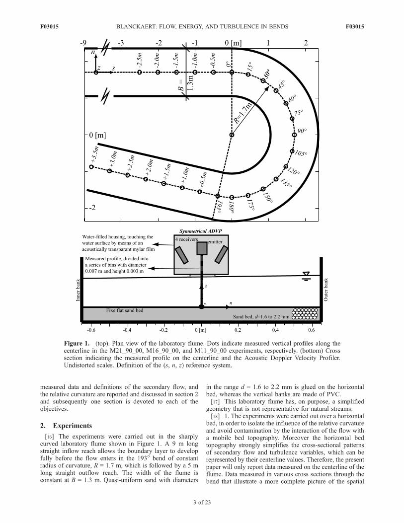
[16] The experiments were carried out in the sharplycurved laboratory flume shown in Figure 1. A 9 m longstraight inflow reach allows the boundary layer to developfully before the flow enters in the 193� bend of constantradius of curvature, R = 1.7 m, which is followed by a 5 mlong straight outflow reach. The width of the flume isconstant at B = 1.3 m. Quasi-uniform sand with diameters

in the range d = 1.6 to 2.2 mm is glued on the horizontalbed, whereas the vertical banks are made of PVC.[17] This laboratory flume has, on purpose, a simplified

geometry that is not representative for natural streams:[18] 1. The experiments were carried out over a horizontal

bed, in order to isolate the influence of the relative curvatureand avoid contamination by the interaction of the flow witha mobile bed topography. Moreover the horizontal bedtopography strongly simplifies the cross-sectional patternsof secondary flow and turbulence variables, which can berepresented by their centerline values. Therefore, the presentpaper will only report data measured on the centerline of theflume. Data measured in various cross sections through thebend that illustrate a more complete picture of the spatial

Figure 1. (top). Plan view of the laboratory flume. Dots indicate measured vertical profiles along thecenterline in the M21_90_00, M16_90_00, and M11_90_00 experiments, respectively. (bottom) Crosssection indicating the measured profile on the centerline and the Acoustic Doppler Velocity Profiler.Undistorted scales. Definition of the (s, n, z) reference system.


3 of 23

F03015

evolution of the hydrodynamics and that demonstrate therepresentativeness of centerline data have been reported byZeng et al. [2008]. More three-dimensional velocity datacan be obtained from the author.[19] 2. The single-bend geometry is characterized by

discontinuities in radius of curvature at the bend entry andexit, which are not representative for natural meander bends,but allow investigating in an isolated way the adaptation ofthe flow to changes in curvature as well as the recovery ofthe flow when the curvature vanishes.[20] 3. The geometric simplicity makes for easier com-

parison with models.[21] The geometric curvature in an open-channel bend

depends on the centerline radius of curvature, R, the widthof the flow, B and the depth of the flow, H, which can becombined into two independent dimensionless parameters,such as H/R and B/R. In natural streams R, B and H arecorrelated according to Leopold et al. [1960] and curvaturecan therefore be parameterized by one of the dimensionlessparameters. Field studies typically make use of the dimen-sionless curvature ratio B/R. The parameters R, B and H areobviously not correlated in laboratory flumes. Since theparameter H/R is the principal curvature parameter inmodels for secondary flow, advective velocity distribution,transverse bed slope or mixing in open-channel bends (seesection 1), it has been adopted in the present paper toparameterize relative curvature. All subsequent referencesto ‘‘curvature’’ or ‘‘relative curvature’’ mean H/R and notB/R. The reported experiments were designed so as to varythe overall averaged flow depth, ~H and the relative curva-ture ~H /R, while keeping the bulk flow velocity, ~U = Q/B ~Habout constant.[22] Data are represented and analyzed in a curvilinear

reference system (s, n, z) with curvilinear s axis in stream-wise direction along the centerline and taking its origin atthe bend entry, transverse n axis to the left and verticallyupward z axis (Figure 1). The transverse velocity compo-nent, vn, is decomposed as [Blanckaert and de Vriend, 2003,Figure 1]

vn ¼ Un þ vn � Unð Þ ð1Þ

The depth-averaged transverse velocity Un representstranslatory cross flow, whereas (vn � Un) represents thetransverse component of the curvature-induced secondaryflow, which is often called spiral flow, helical flow or cross-stream circulation. This decomposition of the transversevelocity and definition of the secondary flow are typical forlaboratory studies. In field studies, secondary flow is oftendifferently defined as the flow component perpendicular tothe local depth-averaged flow.

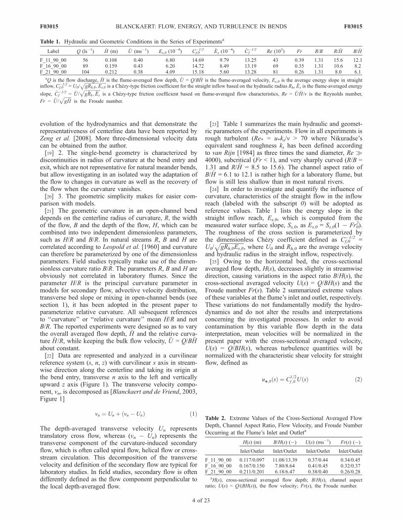
[23] Table 1 summarizes the main hydraulic and geomet-ric parameters of the experiments. Flow in all experiments isrough turbulent (Re* = u*ks/v > 70 where Nikuradse’sequivalent sand roughness ks has been defined accordingto van Rijn [1984] as three times the sand diameter, Re �4000), subcritical (Fr < 1), and very sharply curved (R/B =1.31 and R/ ~H = 8.5 to 15.6). The channel aspect ratio ofB/ ~H = 6.1 to 12.1 is rather high for a laboratory flume, butflow is still less shallow than in most natural rivers.[24] In order to investigate and quantify the influence of

curvature, characteristics of the straight flow in the inflowreach (labeled with the subscript 0) will be adopted asreference values. Table 1 lists the energy slope in thestraight inflow reach, Es,0, which is computed from themeasured water surface slope, Ss,0, as Es,0 = Ss,0(1 � Fr0

2).The roughness of the cross section is parameterized bythe dimensionless Chezy coefficient defined as Cf,0

�1/2 =U0/

ffiffiffiffiffiffiffiffiffiffiffiffiffiffiffiffiffigRh;0Es;0

p, where U0 and Rh,0 are the average velocity

and hydraulic radius in the straight inflow, respectively.[25] Owing to the horizontal bed, the cross-sectional

averaged flow depth, H(s), decreases slightly in streamwisedirection, causing variations in the aspect ratio B/H(s), thecross-sectional averaged velocity U(s) = Q/BH(s) and theFroude number Fr(s). Table 2 summarized extreme valuesof these variables at the flume’s inlet and outlet, respectively.These variations do not fundamentally modify the hydro-dynamics and do not alter the results and interpretationsconcerning the investigated processes. In order to avoidcontamination by this variable flow depth in the datainterpretation, mean velocities will be normalized in thepresent paper with the cross-sectional averaged velocity,U(s) = Q/BH(s), whereas turbulence quantities will benormalized with the characteristic shear velocity for straightflow, defined as

u*;0

ðsÞ ¼ C1=2f ;0 UðsÞ ð2Þ

Table 1. Hydraulic and Geometric Conditions in the Series of Experimentsa

Label Q (ls�1) ~H (m) ~U (ms�1) Es,0 (10�4) Cf,0

�1/2 ~Es (10�4) ~Cf

�1/2 Re (103) Fr R/B R/ ~H B/ ~H

F_11_90_00 56 0.108 0.40 6.80 14.69 9.79 13.25 43 0.39 1.31 15.6 12.1F_16_90_00 89 0.159 0.43 6.20 14.72 8.49 13.19 69 0.35 1.31 10.6 8.2F_21_90_00 104 0.212 0.38 4.09 15.18 5.60 13.28 81 0.26 1.31 8.0 6.1

aQ is the flow discharge, ~H is the flume-averaged flow depth, ~U = Q/B ~H is the flume-averaged velocity, Es,0 is the average energy slope in straightinflow, Cf,0

�1/2 = U0/ffiffiffiffiffiffiffiffiffiffiffiffiffiffiffiffiffiffiffiffigRh;0;Es;0

pis a Chezy-type friction coefficient for the straight inflow based on the hydraulic radius Rh, ~Es is the flume-averaged energy

slope, ~Cf�1/2 = ~U /

ffiffiffiffiffiffiffiffiffiffiffiffiffiffiffig~Rh; ~Es

pis a Chezy-type friction coefficient based on flume-averaged flow characteristics, Re = ~U ~H /v is the Reynolds number,

Fr = ~U /ffiffiffiffiffiffiffig ~H

pis the Froude number.

Table 2. Extreme Values of the Cross-Sectional Averaged Flow

Depth, Channel Aspect Ratio, Flow Velocity, and Froude Number

Occurring at the Flume’s Inlet and Outleta

H(s) (m) B/H(s) (�) U(s) (ms�1) Fr(s) (�)

Inlet/Outlet Inlet/Outlet Inlet/Outlet Inlet/Outlet

F_11_90_00 0.117/0.097 11.08/13.39 0.37/0.44 0.34/0.45F_16_90_00 0.167/0.150 7.80/8.64 0.41/0.45 0.32/0.37F_21_90_00 0.211/0.201 6.18/6.47 0.38/0.40 0.26/0.28

aH(s), cross-sectional averaged flow depth; B/H(s), channel aspectratio; U(s) = Q/(BH(s)), the flow velocity; Fr(s), the Froude number.


4 of 23

F03015

It should be noted that different methods can be applied toestimate the shear velocity in straight uniform flow (energyslope, logarithmic velocity profile, shear stress profile,turbulent kinetic energy). Nezu and Nakagawa [1993]describe these methods and estimate the uncertainty in theestimates as O(30%), which is in agreement with resultsfrom the presented experiments. Such an uncertainty isconsiderable, especially since most turbulence quantities arenormalized with u*,0

2 .[26] Measurements of the water surface topography were

made by moving a set of 8 acoustic limnimeters mounted ona carriage along the flume. The limnimeters were mountedin the transverse positions n = [�0.6, �0.5, �0.3, �0.1, 0.1,0.3, 0.5, 0.6] m. In streamwise direction, the measuring gridwas refined near the bend entry and exit where importantwater surface gradients exist owing to the discontinuity incurvature. Measurements were made in the cross sections inthe bend at [0, 5, 10, 15, 20, 25, 30, 35, 40, 50, 60, 70, 80,90, 100, 110, 120, 130, 140, 150, 160, 165, 170, 175, 180,185, 190, 193]� and in the straight outflow at [0.3, 0.5, 0.8,1, 1.3, 1.5, 1.8, 2, 2.5, 3, 3.5, 4] m downstream of the bend.In order to estimate accurately the small water surface andenergy slopes in the straight inflow reach, a refined mea-suring grid was adopted with 24 transverse measuringpositions in cross sections spaced by 0.1 m in the reachfrom 7.5 m upstream of the bend entrance onto the bendentrance.[27] Nonintrusive measurements of velocity profiles were

carried out with an Acoustic Doppler Velocity Profiler(ADVP) on the centerline at 2.5 m, 2.0 m, 1.5 m, 1.0 m,0.5 m upstream of the bend, every 15� in the bend and every0.5 m in the straight outflow reach (Figure 1). The workingprinciple of the ADVP has been reported by Lemmin andRolland [1997], Hurther and Lemmin [1998], Blanckaertand Graf [2001], and Blanckaert and Lemmin [2006]. The

ADVP consists of a central emitter, surrounded by fourreceivers, placed in a water filled box that touches the watersurface by means of an acoustically transparent mylar film(Figure 1). It measures profiles of the quasi-instantaneousvelocity vector, ~v(t) = (vs, vn, vz)(t), from which the time-averaged velocity vector, ~v = (vs, vn, vz), the Reynoldsstresses, �rv 0i v

0j (i, j = s, n, z) and higher-order turbulent

correlations can be computed. Measurements were madewith a sampling frequency of 31.25 Hz and a samplingperiod of 90 s. The series of experiments is designed tomake optimal use of the ADVP’s strong points, as explainedby K. Blanckaert (submitted manuscript, 2009).[28] Blanckaert (submitted manuscript, 2009) reports and

illustrates the data treatment procedures applied to trans-form the raw data obtained by the ADVP into a formatappropriate for data analysis and presentation. Moreover, heestimates the uncertainty in the experimental data as fol-lows: streamwise velocity vs: 4%, cross-stream velocities(vn, vz): 10%, shear velocity u*: 30%, turbulent shearstresses: 15%, turbulent normal stresses and turbulent ki-netic energy: 20% (accounting for noise corruption of highfrequency fluctuations by means of the method reported byBlanckaert and Lemmin [2006]), turbulence production rate:50% and turbulence dissipation rate: 100%.[29] The accuracy in the ADVP measurements is reduced

near the flow boundaries. At the water surface, the ADVPhousing (Figure 1) perturbs the flow in a region of about2 cm (about 10 to 15% of the flow depth in our experi-ments). In a flow layer of about 2 cm near solid boundaries,the ADVP seems to underestimate turbulent characteristics,which is tentatively attributed to the high velocity gradientswithin the measuring volume and/or to parasitical echoesfrom the solid boundary [Hurther and Lemmin, 2001].ADVP measurements seem to underestimate systematicallythe vertical velocity fluctuations.

3. Experimental Observations

3.1. Water Surface Topography

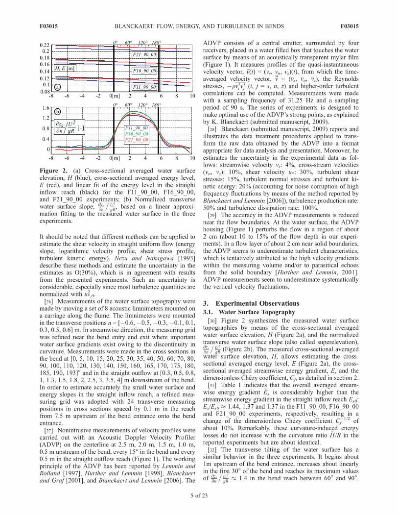
[30] Figure 2 synthesizes the measured water surfacetopographies by means of the cross-sectional averagedwater surface elevation, H (Figure 2a), and the normalizedtransverse water surface slope (also called superelevation),@zs@n

�U2

gR(Figure 2b). The measured cross-sectional averaged

water surface elevation, H, allows estimating the cross-sectional averaged energy level, E (Figure 2a), the cross-sectional averaged streamwise energy gradient, Es and thedimensionless Chezy coefficient, Cf, as detailed in section 2.[31] Table 1 indicates that the overall averaged stream-

wise energy gradient ~Es is considerably higher than thestreamwise energy gradient in the straight inflow reach Es0:~Es/Es0 � 1.44, 1.37 and 1.37 in the F11_90_00, F16_90_00and F21_90_00 experiments, respectively, resulting in achange of the dimensionless Chezy coefficient Cf

�1/2 ofabout 10%. Remarkably, these curvature-induced energylosses do not increase with the curvature ratio ~H /R in thereported experiments but are about identical.[32] The transverse tilting of the water surface has a

similar behavior in the three experiments. It begins about1m upstream of the bend entrance, increases about linearlyin the first 30� of the bend and reaches its maximum valuesof @zs

@n

�U 2

gR� 1.4 in the bend reach between 60� and 90�.

Figure 2. (a) Cross-sectional averaged water surfaceelevation, H (blue), cross-sectional averaged energy level,E (red), and linear fit of the energy level in the straightinflow reach (black) for the F11_90_00, F16_90_00,and F21_90_00 experiments; (b) Normalized transversewater surface slope, @zs

@n

�U2

gR, based on a linear approxi-

mation fitting to the measured water surface in the threeexperiments.


5 of 23

F03015

Remarkably, the transverse tilting of the water surface slopedoes subsequently not remain constant in this long bendedreach of constant curvature, but decreases and it is reducedat the bend exit to about half of its maximum value in thebend, indicating that the transverse tilting of the watersurface overshoots its equilibrium value in the first part ofthe bend. The transverse tilting decays quickly downstreamof the bend and is negligible about 1 m downstream of thebend exit. These observations deviate from the ‘‘classical’’description of the transversal tilting as adapting very quicklyto curvature changes and being constant in a bend of con-stant radius of curvature.

3.2. Mean Flow Characteristics Along the Centerline

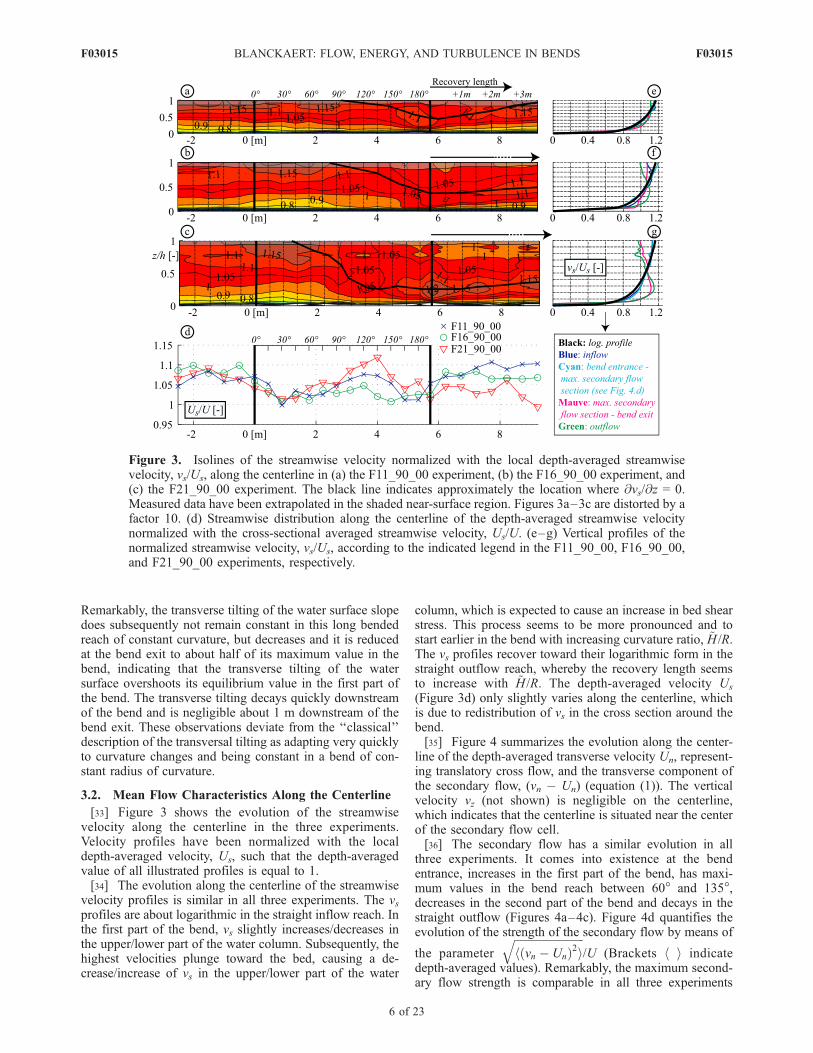
[33] Figure 3 shows the evolution of the streamwisevelocity along the centerline in the three experiments.Velocity profiles have been normalized with the localdepth-averaged velocity, Us, such that the depth-averagedvalue of all illustrated profiles is equal to 1.[34] The evolution along the centerline of the streamwise

velocity profiles is similar in all three experiments. The vsprofiles are about logarithmic in the straight inflow reach. Inthe first part of the bend, vs slightly increases/decreases inthe upper/lower part of the water column. Subsequently, thehighest velocities plunge toward the bed, causing a de-crease/increase of vs in the upper/lower part of the water

column, which is expected to cause an increase in bed shearstress. This process seems to be more pronounced and tostart earlier in the bend with increasing curvature ratio, ~H /R.The vs profiles recover toward their logarithmic form in thestraight outflow reach, whereby the recovery length seemsto increase with ~H /R. The depth-averaged velocity Us

(Figure 3d) only slightly varies along the centerline, whichis due to redistribution of vs in the cross section around thebend.[35] Figure 4 summarizes the evolution along the center-

line of the depth-averaged transverse velocity Un, represent-ing translatory cross flow, and the transverse component ofthe secondary flow, (vn � Un) (equation (1)). The verticalvelocity vz (not shown) is negligible on the centerline,which indicates that the centerline is situated near the centerof the secondary flow cell.[36] The secondary flow has a similar evolution in all

three experiments. It comes into existence at the bendentrance, increases in the first part of the bend, has maxi-mum values in the bend reach between 60� and 135�,decreases in the second part of the bend and decays in thestraight outflow (Figures 4a–4c). Figure 4d quantifies theevolution of the strength of the secondary flow by means of

the parameter

ffiffiffiffiffiffiffiffiffiffiffiffiffiffiffiffiffiffiffiffiffiffiffiffiffihðvn � UnÞ2i

q/U (Brackets h i indicate

depth-averaged values). Remarkably, the maximum second-ary flow strength is comparable in all three experiments

Figure 3. Isolines of the streamwise velocity normalized with the local depth-averaged streamwisevelocity, vs/Us, along the centerline in (a) the F11_90_00 experiment, (b) the F16_90_00 experiment, and(c) the F21_90_00 experiment. The black line indicates approximately the location where @vs/@z = 0.Measured data have been extrapolated in the shaded near-surface region. Figures 3a–3c are distorted by afactor 10. (d) Streamwise distribution along the centerline of the depth-averaged streamwise velocitynormalized with the cross-sectional averaged streamwise velocity, Us/U. (e–g) Vertical profiles of thenormalized streamwise velocity, vs/Us, according to the indicated legend in the F11_90_00, F16_90_00,and F21_90_00 experiments, respectively.


6 of 23

F03015

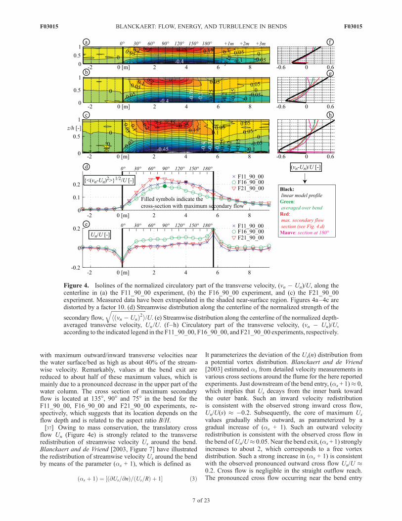
with maximum outward/inward transverse velocities nearthe water surface/bed as high as about 40% of the stream-wise velocity. Remarkably, values at the bend exit arereduced to about half of these maximum values, which ismainly due to a pronounced decrease in the upper part of thewater column. The cross section of maximum secondaryflow is located at 135�, 90� and 75� in the bend for theF11_90_00, F16_90_00 and F21_90_00 experiments, re-spectively, which suggests that its location depends on theflow depth and is related to the aspect ratio B/H.[37] Owing to mass conservation, the translatory cross

flow Un (Figure 4e) is strongly related to the transverseredistribution of streamwise velocity Us around the bend.Blanckaert and de Vriend [2003, Figure 7] have illustratedthe redistribution of streamwise velocity Us around the bendby means of the parameter (as + 1), which is defined as

as þ 1ð Þ ¼ @Us=@nð Þ= Us=Rð Þ þ 1½ � ð3Þ

It parameterizes the deviation of the Us(n) distribution froma potential vortex distribution. Blanckaert and de Vriend[2003] estimated as from detailed velocity measurements invarious cross sections around the flume for the here reportedexperiments. Just downstream of the bend entry, (as + 1)� 0,which implies that Us decays from the inner bank towardthe outer bank. Such an inward velocity redistributionis consistent with the observed strong inward cross flow,Un/U(s) � �0.2. Subsequently, the core of maximum Us

values gradually shifts outward, as parameterized by agradual increase of (as + 1). Such an outward velocityredistribution is consistent with the observed cross flow inthe bend ofUn/U� 0.05. Near the bend exit, (as + 1) stronglyincreases to about 2, which corresponds to a free vortexdistribution. Such a strong increase in (as + 1) is consistentwith the observed pronounced outward cross flow Un/U �0.2. Cross flow is negligible in the straight outflow reach.The pronounced cross flow occurring near the bend entry

Figure 4. Isolines of the normalized circulatory part of the transverse velocity, (vn � Un)/U, along thecenterline in (a) the F11_90_00 experiment, (b) the F16_90_00 experiment, and (c) the F21_90_00experiment. Measured data have been extrapolated in the shaded near-surface region. Figures 4a–4c aredistorted by a factor 10. (d) Streamwise distribution along the centerline of the normalized strength of the

secondary flow,

ffiffiffiffiffiffiffiffiffiffiffiffiffiffiffiffiffiffiffiffiffiffiffiffiffihðvn � UnÞ2i

q/U. (e) Streamwise distribution along the centerline of the normalized depth-

averaged transverse velocity, Un /U. (f–h) Circulatory part of the transverse velocity, (vn � Un)/U,according to the indicated legend in the F11_90_00, F16_90_00, and F21_90_00 experiments, respectively.


7 of 23

F03015

and exit are due to the discontinuities in curvature andare therefore not representative of natural river bends.

3.3. Turbulence Characteristics Along the Centerline

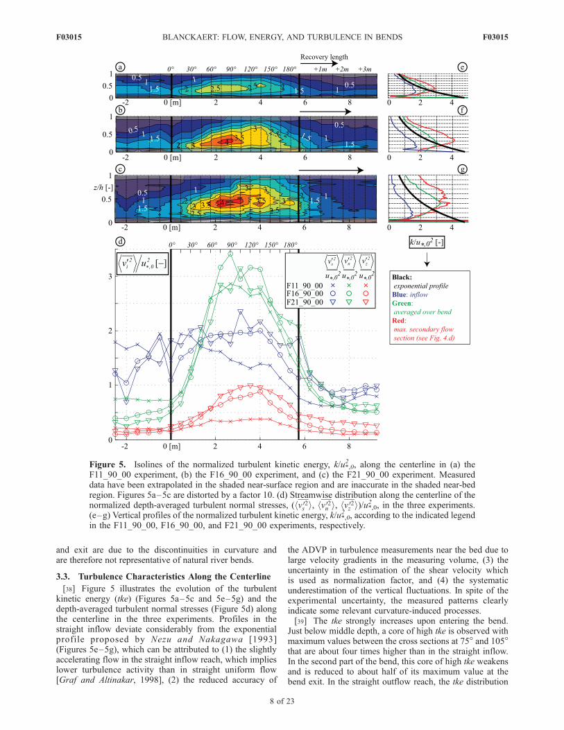
[38] Figure 5 illustrates the evolution of the turbulentkinetic energy (tke) (Figures 5a–5c and 5e–5g) and thedepth-averaged turbulent normal stresses (Figure 5d) alongthe centerline in the three experiments. Profiles in thestraight inflow deviate considerably from the exponentialprofile proposed by Nezu and Nakagawa [1993](Figures 5e–5g), which can be attributed to (1) the slightlyaccelerating flow in the straight inflow reach, which implieslower turbulence activity than in straight uniform flow[Graf and Altinakar, 1998], (2) the reduced accuracy of

the ADVP in turbulence measurements near the bed due tolarge velocity gradients in the measuring volume, (3) theuncertainty in the estimation of the shear velocity whichis used as normalization factor, and (4) the systematicunderestimation of the vertical fluctuations. In spite of theexperimental uncertainty, the measured patterns clearlyindicate some relevant curvature-induced processes.[39] The tke strongly increases upon entering the bend.

Just below middle depth, a core of high tke is observed withmaximum values between the cross sections at 75� and 105�that are about four times higher than in the straight inflow.In the second part of the bend, this core of high tke weakensand is reduced to about half of its maximum value at thebend exit. In the straight outflow reach, the tke distribution

Figure 5. Isolines of the normalized turbulent kinetic energy, k/u*,02 , along the centerline in (a) the

F11_90_00 experiment, (b) the F16_90_00 experiment, and (c) the F21_90_00 experiment. Measureddata have been extrapolated in the shaded near-surface region and are inaccurate in the shaded near-bedregion. Figures 5a–5c are distorted by a factor 10. (d) Streamwise distribution along the centerline of thenormalized depth-averaged turbulent normal stresses, (hv 02s i, hv 02n i, hv 02z i)/u*,0

2 , in the three experiments.(e–g) Vertical profiles of the normalized turbulent kinetic energy, k/u*,0

2 , according to the indicated legendin the F11_90_00, F16_90_00, and F21_90_00 experiments, respectively.


8 of 23

F03015

recovers toward its straight uniform flow pattern. Therecovery length seems to increase with flow depth asindicated by the isoline patterns in Figures 5a–5c. Althoughthe streamwise and vertical turbulent normal stresses in-

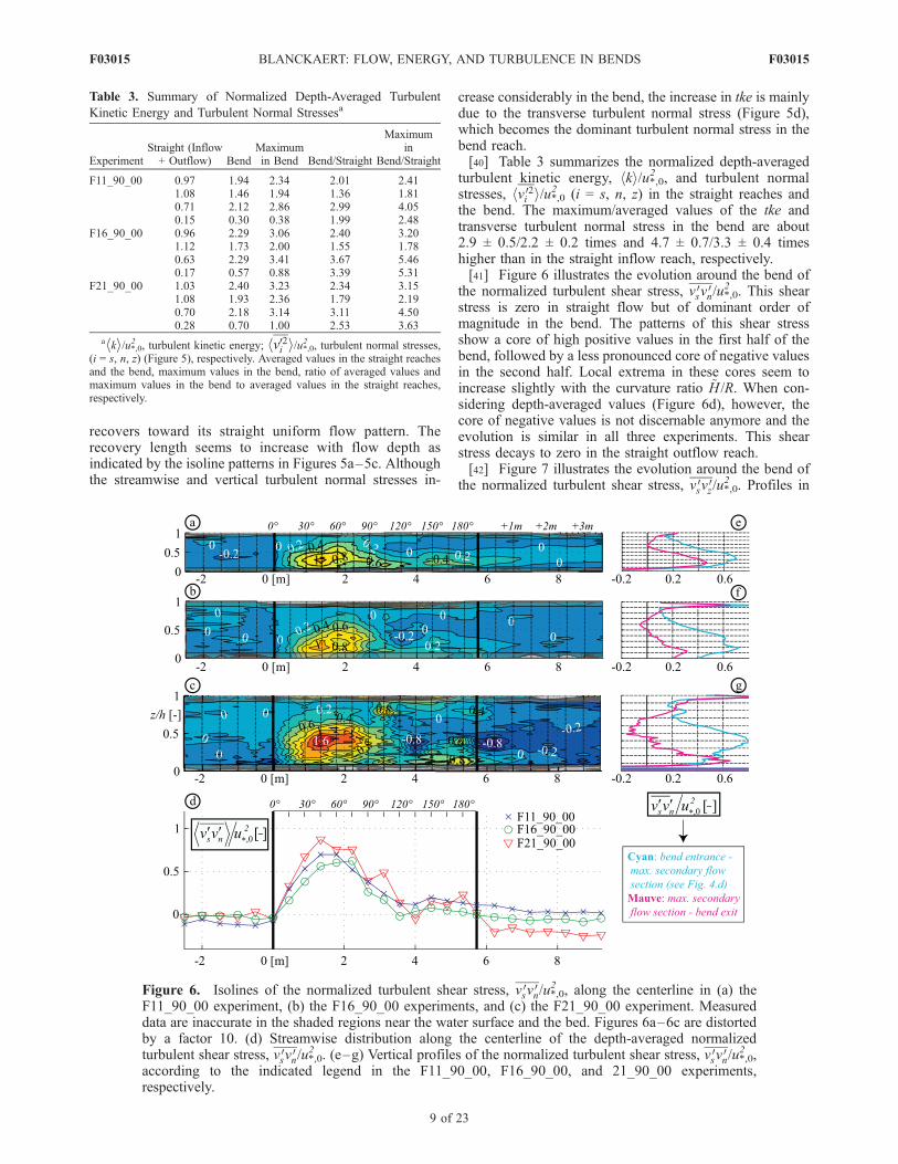
crease considerably in the bend, the increase in tke is mainlydue to the transverse turbulent normal stress (Figure 5d),which becomes the dominant turbulent normal stress in thebend reach.[40] Table 3 summarizes the normalized depth-averaged

turbulent kinetic energy, hki/u*,02 , and turbulent normalstresses, hv 02i i/u*,0

2 (i = s, n, z) in the straight reaches andthe bend. The maximum/averaged values of the tke andtransverse turbulent normal stress in the bend are about2.9 ± 0.5/2.2 ± 0.2 times and 4.7 ± 0.7/3.3 ± 0.4 timeshigher than in the straight inflow reach, respectively.[41] Figure 6 illustrates the evolution around the bend of

the normalized turbulent shear stress, v 0sv0n/u*,0

2 . This shearstress is zero in straight flow but of dominant order ofmagnitude in the bend. The patterns of this shear stressshow a core of high positive values in the first half of thebend, followed by a less pronounced core of negative valuesin the second half. Local extrema in these cores seem toincrease slightly with the curvature ratio ~H /R. When con-sidering depth-averaged values (Figure 6d), however, thecore of negative values is not discernable anymore and theevolution is similar in all three experiments. This shearstress decays to zero in the straight outflow reach.[42] Figure 7 illustrates the evolution around the bend of

the normalized turbulent shear stress, v 0sv0z/u*,0

2 . Profiles in

Table 3. Summary of Normalized Depth-Averaged Turbulent

Kinetic Energy and Turbulent Normal Stressesa

ExperimentStraight (Inflow+ Outflow) Bend

Maximumin Bend Bend/Straight

Maximumin

Bend/Straight

F11_90_00 0.97 1.94 2.34 2.01 2.411.08 1.46 1.94 1.36 1.810.71 2.12 2.86 2.99 4.050.15 0.30 0.38 1.99 2.48

F16_90_00 0.96 2.29 3.06 2.40 3.201.12 1.73 2.00 1.55 1.780.63 2.29 3.41 3.67 5.460.17 0.57 0.88 3.39 5.31

F21_90_00 1.03 2.40 3.23 2.34 3.151.08 1.93 2.36 1.79 2.190.70 2.18 3.14 3.11 4.500.28 0.70 1.00 2.53 3.63

ahki/u*,02 , turbulent kinetic energy; hv02i i/u*,02 , turbulent normal stresses,(i = s, n, z) (Figure 5), respectively. Averaged values in the straight reachesand the bend, maximum values in the bend, ratio of averaged values andmaximum values in the bend to averaged values in the straight reaches,respectively.

Figure 6. Isolines of the normalized turbulent shear stress, v 0sv0n/u*,0

2 , along the centerline in (a) theF11_90_00 experiment, (b) the F16_90_00 experiments, and (c) the F21_90_00 experiment. Measureddata are inaccurate in the shaded regions near the water surface and the bed. Figures 6a–6c are distortedby a factor 10. (d) Streamwise distribution along the centerline of the depth-averaged normalizedturbulent shear stress, v 0sv

0n/u*,0

2 . (e–g) Vertical profiles of the normalized turbulent shear stress, v 0sv0n/u*,0

2 ,according to the indicated legend in the F11_90_00, F16_90_00, and 21_90_00 experiments,respectively.


9 of 23

F03015

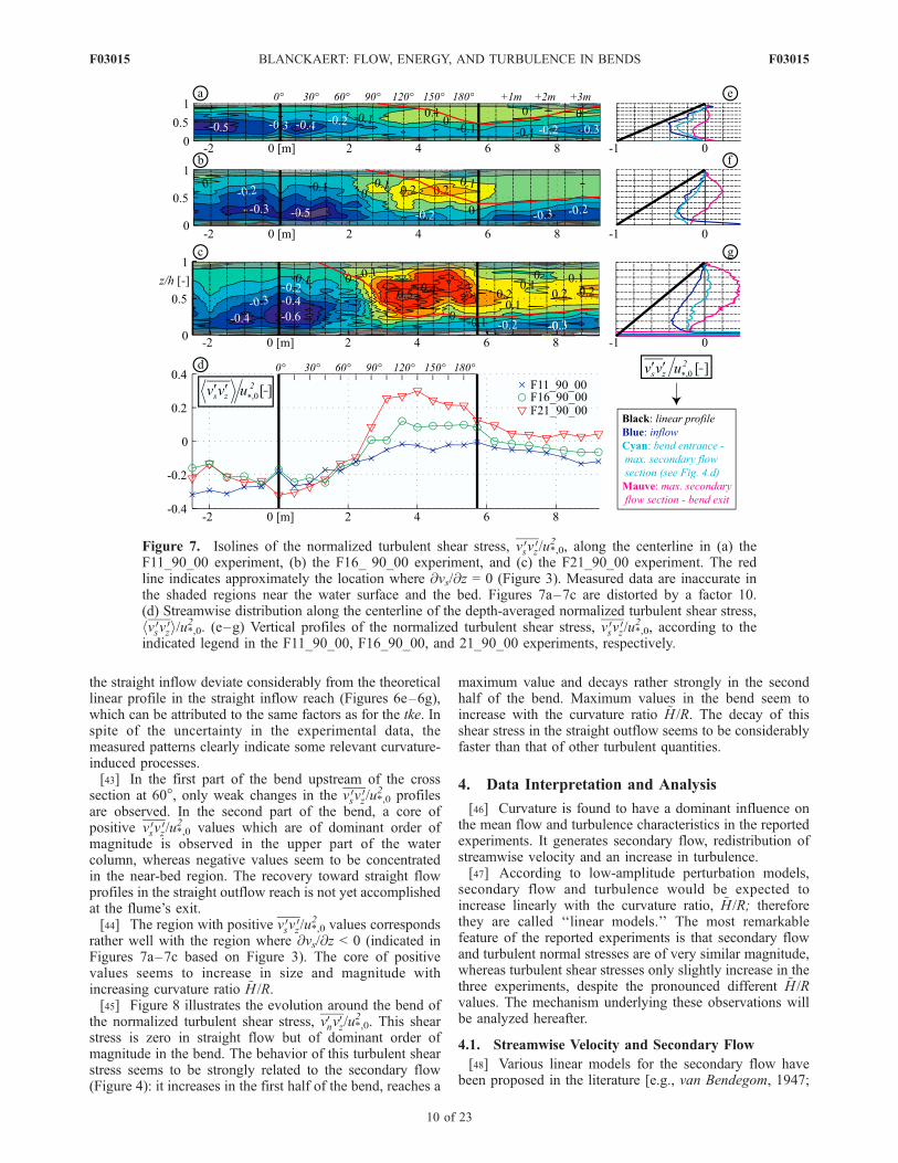
the straight inflow deviate considerably from the theoreticallinear profile in the straight inflow reach (Figures 6e–6g),which can be attributed to the same factors as for the tke. Inspite of the uncertainty in the experimental data, themeasured patterns clearly indicate some relevant curvature-induced processes.[43] In the first part of the bend upstream of the cross

section at 60�, only weak changes in the v 0sv0z/u*,0

2 profilesare observed. In the second part of the bend, a core ofpositive v 0sv

0z/u*,0

2 values which are of dominant order ofmagnitude is observed in the upper part of the watercolumn, whereas negative values seem to be concentratedin the near-bed region. The recovery toward straight flowprofiles in the straight outflow reach is not yet accomplishedat the flume’s exit.[44] The region with positive v 0sv

0z/u*,0

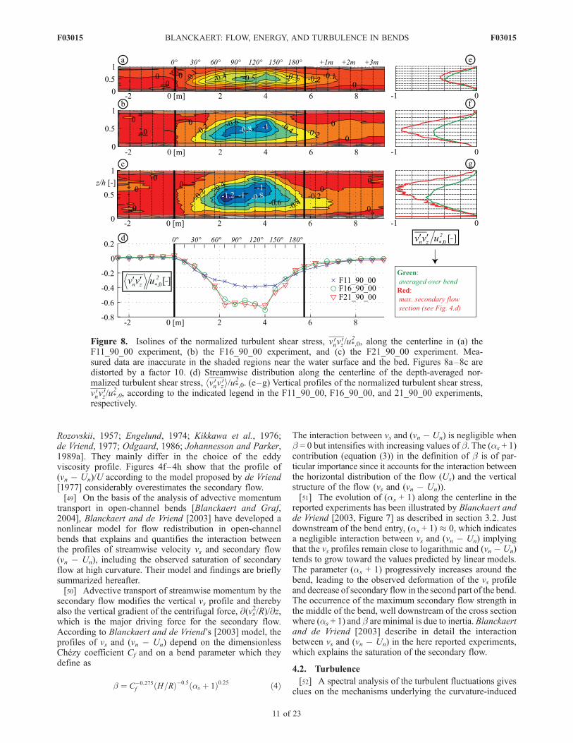
2 values correspondsrather well with the region where @vs/@z < 0 (indicated inFigures 7a–7c based on Figure 3). The core of positivevalues seems to increase in size and magnitude withincreasing curvature ratio ~H /R.[45] Figure 8 illustrates the evolution around the bend of

the normalized turbulent shear stress, v0nv0z/u*,0

2 . This shearstress is zero in straight flow but of dominant order ofmagnitude in the bend. The behavior of this turbulent shearstress seems to be strongly related to the secondary flow(Figure 4): it increases in the first half of the bend, reaches a

maximum value and decays rather strongly in the secondhalf of the bend. Maximum values in the bend seem toincrease with the curvature ratio ~H /R. The decay of thisshear stress in the straight outflow seems to be considerablyfaster than that of other turbulent quantities.

4. Data Interpretation and Analysis

[46] Curvature is found to have a dominant influence onthe mean flow and turbulence characteristics in the reportedexperiments. It generates secondary flow, redistribution ofstreamwise velocity and an increase in turbulence.[47] According to low-amplitude perturbation models,

secondary flow and turbulence would be expected toincrease linearly with the curvature ratio, ~H /R; thereforethey are called ‘‘linear models.’’ The most remarkablefeature of the reported experiments is that secondary flowand turbulent normal stresses are of very similar magnitude,whereas turbulent shear stresses only slightly increase in thethree experiments, despite the pronounced different ~H /Rvalues. The mechanism underlying these observations willbe analyzed hereafter.

4.1. Streamwise Velocity and Secondary Flow

[48] Various linear models for the secondary flow havebeen proposed in the literature [e.g., van Bendegom, 1947;

Figure 7. Isolines of the normalized turbulent shear stress, v 0sv0z/u*,0

2 , along the centerline in (a) theF11_90_00 experiment, (b) the F16_ 90_00 experiment, and (c) the F21_90_00 experiment. The redline indicates approximately the location where @vs/@z = 0 (Figure 3). Measured data are inaccurate inthe shaded regions near the water surface and the bed. Figures 7a–7c are distorted by a factor 10.(d) Streamwise distribution along the centerline of the depth-averaged normalized turbulent shear stress,hv 0sv 0zi/u*,0

2 . (e–g) Vertical profiles of the normalized turbulent shear stress, v 0sv0z/u*,0

2 , according to theindicated legend in the F11_90_00, F16_90_00, and 21_90_00 experiments, respectively.


10 of 23

F03015

Rozovskii, 1957; Engelund, 1974; Kikkawa et al., 1976;de Vriend, 1977; Odgaard, 1986; Johannesson and Parker,1989a]. They mainly differ in the choice of the eddyviscosity profile. Figures 4f–4h show that the profile of(vn � Un)/U according to the model proposed by de Vriend[1977] considerably overestimates the secondary flow.[49] On the basis of the analysis of advective momentum

transport in open-channel bends [Blanckaert and Graf,2004], Blanckaert and de Vriend [2003] have developed anonlinear model for flow redistribution in open-channelbends that explains and quantifies the interaction betweenthe profiles of streamwise velocity vs and secondary flow(vn � Un), including the observed saturation of secondaryflow at high curvature. Their model and findings are brieflysummarized hereafter.[50] Advective transport of streamwise momentum by the

secondary flow modifies the vertical vs profile and therebyalso the vertical gradient of the centrifugal force, @(vs

2/R)/@z,which is the major driving force for the secondary flow.According to Blanckaert and de Vriend’s [2003] model, theprofiles of vs and (vn � Un) depend on the dimensionlessChezy coefficient Cf and on a bend parameter which theydefine as

b ¼ C�0:275f H=Rð Þ�0:5 as þ 1ð Þ0:25 ð4Þ

The interaction between vs and (vn � Un) is negligible whenb = 0 but intensifies with increasing values of b. The (as + 1)contribution (equation (3)) in the definition of b is of par-ticular importance since it accounts for the interaction betweenthe horizontal distribution of the flow (Us) and the verticalstructure of the flow (vs and (vn � Un)).[51] The evolution of (as + 1) along the centerline in the

reported experiments has been illustrated by Blanckaert andde Vriend [2003, Figure 7] as described in section 3.2. Justdownstream of the bend entry, (as + 1) � 0, which indicatesa negligible interaction between vs and (vn � Un) implyingthat the vs profiles remain close to logarithmic and (vn � Un)tends to grow toward the values predicted by linear models.The parameter (as + 1) progressively increases around thebend, leading to the observed deformation of the vs profileand decrease of secondary flow in the second part of the bend.The occurrence of the maximum secondary flow strength inthe middle of the bend, well downstream of the cross sectionwhere (as + 1) and b are minimal is due to inertia. Blanckaertand de Vriend [2003] describe in detail the interactionbetween vs and (vn � Un) in the here reported experiments,which explains the saturation of the secondary flow.

4.2. Turbulence

[52] A spectral analysis of the turbulent fluctuations givesclues on the mechanisms underlying the curvature-induced

Figure 8. Isolines of the normalized turbulent shear stress, v 0nv0z/u*,0

2 , along the centerline in (a) theF11_90_00 experiment, (b) the F16_90_00 experiment, and (c) the F21_90_00 experiment. Mea-sured data are inaccurate in the shaded regions near the water surface and the bed. Figures 8a–8c aredistorted by a factor 10. (d) Streamwise distribution along the centerline of the depth-averaged nor-malized turbulent shear stress, hv 0nv 0zi/u*,0

2 . (e–g) Vertical profiles of the normalized turbulent shear stress,v 0nv

0z/u*,0

2 , according to the indicated legend in the F11_90_00, F16_90_00, and 21_90_00 experiments,respectively.


11 of 23

F03015

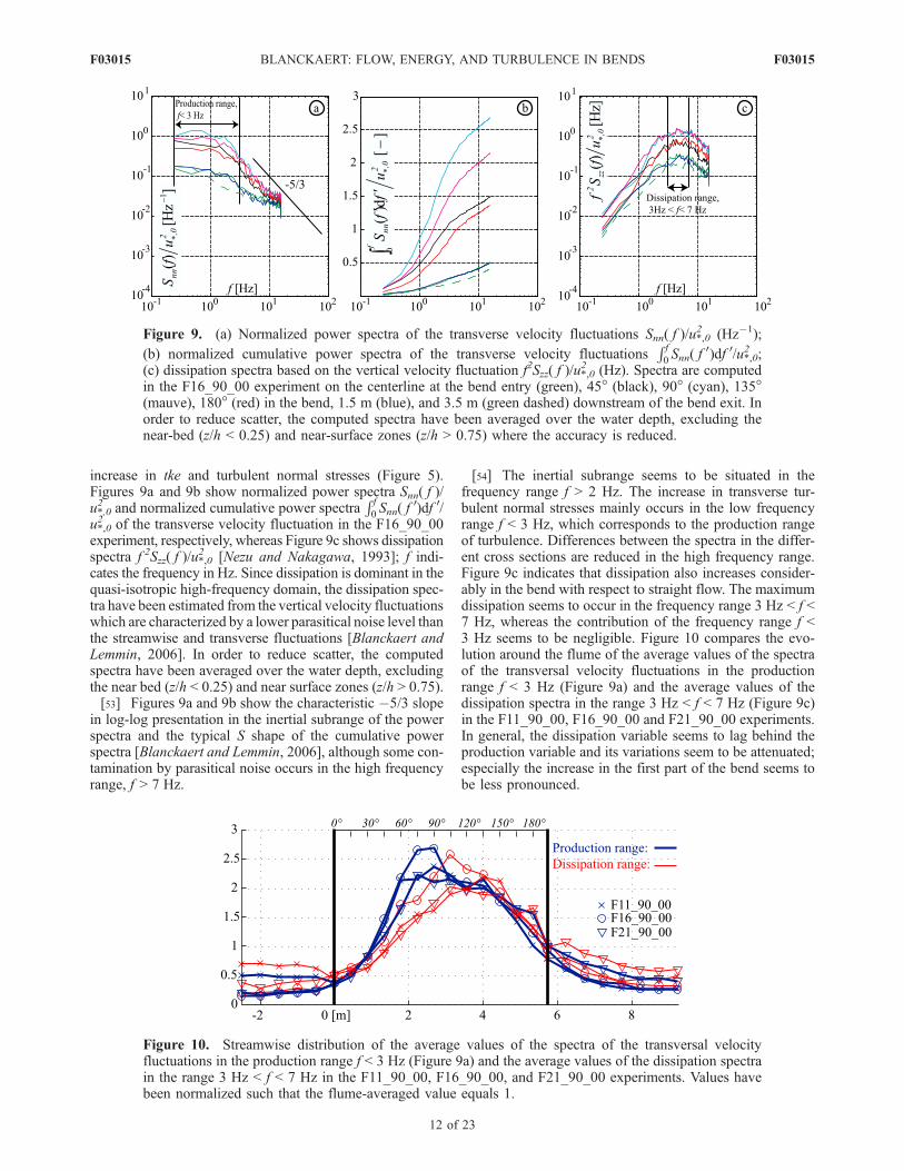
increase in tke and turbulent normal stresses (Figure 5).Figures 9a and 9b show normalized power spectra Snn( f )/u*,02 and normalized cumulative power spectra

R f0Snn( f

0)df 0/u*,02 of the transverse velocity fluctuation in the F16_90_00experiment, respectively, whereas Figure 9c shows dissipationspectra f 2Szz( f )/u*,0

2 [Nezu and Nakagawa, 1993]; f indi-cates the frequency in Hz. Since dissipation is dominant in thequasi-isotropic high-frequency domain, the dissipation spec-tra have been estimated from the vertical velocity fluctuationswhich are characterized by a lower parasitical noise level thanthe streamwise and transverse fluctuations [Blanckaert andLemmin, 2006]. In order to reduce scatter, the computedspectra have been averaged over the water depth, excludingthe near bed (z/h < 0.25) and near surface zones (z/h > 0.75).[53] Figures 9a and 9b show the characteristic �5/3 slope

in log-log presentation in the inertial subrange of the powerspectra and the typical S shape of the cumulative powerspectra [Blanckaert and Lemmin, 2006], although some con-tamination by parasitical noise occurs in the high frequencyrange, f > 7 Hz.

[54] The inertial subrange seems to be situated in thefrequency range f > 2 Hz. The increase in transverse tur-bulent normal stresses mainly occurs in the low frequencyrange f < 3 Hz, which corresponds to the production rangeof turbulence. Differences between the spectra in the differ-ent cross sections are reduced in the high frequency range.Figure 9c indicates that dissipation also increases consider-ably in the bend with respect to straight flow. The maximumdissipation seems to occur in the frequency range 3 Hz < f <7 Hz, whereas the contribution of the frequency range f <3 Hz seems to be negligible. Figure 10 compares the evo-lution around the flume of the average values of the spectraof the transversal velocity fluctuations in the productionrange f < 3 Hz (Figure 9a) and the average values of thedissipation spectra in the range 3 Hz < f < 7 Hz (Figure 9c)in the F11_90_00, F16_90_00 and F21_90_00 experiments.In general, the dissipation variable seems to lag behind theproduction variable and its variations seem to be attenuated;especially the increase in the first part of the bend seems tobe less pronounced.

Figure 9. (a) Normalized power spectra of the transverse velocity fluctuations Snn( f )/u*,02 (Hz�1);

(b) normalized cumulative power spectra of the transverse velocity fluctuationsR f0Snn( f

0)df 0/u*,02 ;

(c) dissipation spectra based on the vertical velocity fluctuation f2Szz( f )/u*,02 (Hz). Spectra are computed

in the F16_90_00 experiment on the centerline at the bend entry (green), 45� (black), 90� (cyan), 135�(mauve), 180� (red) in the bend, 1.5 m (blue), and 3.5 m (green dashed) downstream of the bend exit. Inorder to reduce scatter, the computed spectra have been averaged over the water depth, excluding thenear-bed (z/h < 0.25) and near-surface zones (z/h > 0.75) where the accuracy is reduced.

Figure 10. Streamwise distribution of the average values of the spectra of the transversal velocityfluctuations in the production range f < 3 Hz (Figure 9a) and the average values of the dissipation spectrain the range 3 Hz < f < 7 Hz in the F11_90_00, F16_90_00, and F21_90_00 experiments. Values havebeen normalized such that the flume-averaged value equals 1.


12 of 23

F03015

[55] These observations are in agreement with theenergy cascade concept of turbulence: tke is generated inthe low frequency range through the interaction betweenthe time-averaged flow and large turbulent structures.While being advected in streamwise direction by the flow,these large turbulent structures disintegrate in smallerstructures accompanied by an increase in frequency andin dissipation rate. On the basis of these observations, thefurther analysis of the mechanisms underlying the in-creased tke and turbulent normal stresses (Figure 5) willconsider the evolution around the flume of the turbulenceproduction rate (Figure 11) and the turbulence dissipationrate (Figure 12). The turbulence production rate is definedby [Hinze, 1975, chap. 1–13]

P ¼ � v 02s � 2

3k

� �ess þ v 02n � 2

3k

� �enn þ v 02z � 2

3k

� �ezz

�

þ 2v 0sv0nesn þ 2v 0sv

0zesz þ 2v 0nv

0zenz

ð5Þ

P ¼ P ss þ P nn þ P zz þ P sn þ P sz þ P nz ð6Þ

The definition of the strain rates, ejk (j, k = s, n, z),according to Batchelor [1967, p. 600] and the

applied estimation based on the measured data aregiven by

ess ¼1

1þ n=R

@vs@s

þ 1

1þ n=R

vn

R� @vs

@sþ vn

R

enn ¼@vn@n

� 0

ezz ¼@vz@z

� 0

esn ¼1

2

1

1þ n=R

@vn@s

þ @vs@n

� 1

1þ n=R

vs

R

� �� 1

2

@vn@s

þ as

vs

R� vs

R

� �

esz ¼1

2

1

1þ n=R

@vz@s

þ @vs@z

� �� 1

2

@vz@s

þ @vs@z

� �

enz ¼1

2

@vz@n

þ @vn@z

� �� 1

2

@vn@z

9>>>>>>>>>>>>>>>>>>>>=>>>>>>>>>>>>>>>>>>>>;ð7Þ

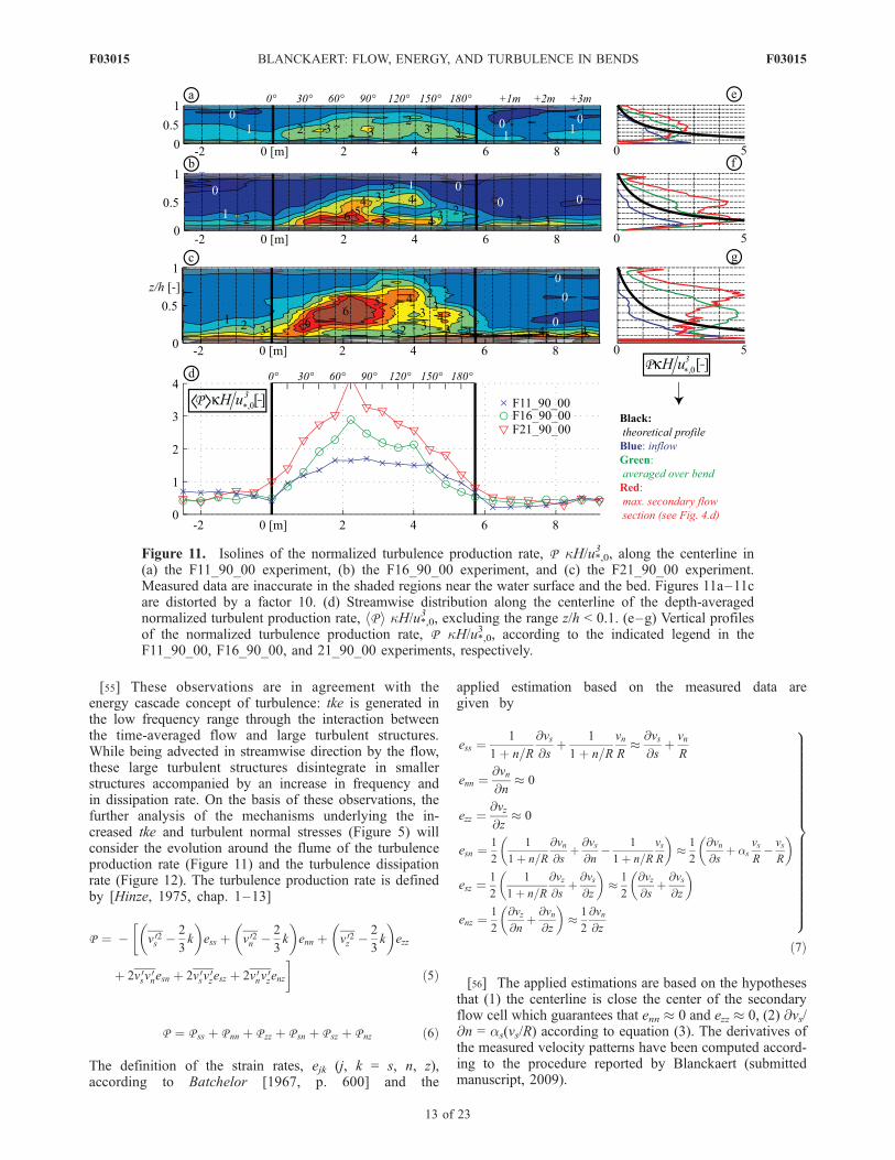
[56] The applied estimations are based on the hypothesesthat (1) the centerline is close the center of the secondaryflow cell which guarantees that enn � 0 and ezz � 0, (2) @vs/@n = as(vs/R) according to equation (3). The derivatives ofthe measured velocity patterns have been computed accord-ing to the procedure reported by Blanckaert (submittedmanuscript, 2009).

Figure 11. Isolines of the normalized turbulence production rate, P kH/u*,03 , along the centerline in

(a) the F11_90_00 experiment, (b) the F16_90_00 experiment, and (c) the F21_90_00 experiment.Measured data are inaccurate in the shaded regions near the water surface and the bed. Figures 11a–11care distorted by a factor 10. (d) Streamwise distribution along the centerline of the depth-averagednormalized turbulent production rate, hP i kH/u*,03 , excluding the range z/h < 0.1. (e–g) Vertical profilesof the normalized turbulence production rate, P kH/u*,0

3 , according to the indicated legend in theF11_90_00, F16_90_00, and 21_90_00 experiments, respectively.


13 of 23

F03015

[57] Agreement with theoretical profiles [Nezu andNakagawa, 1993] in the straight inflow is satisfactorily(Figures 11e–11g). The accuracy is reduced in the lowerpart of the water column, z/h < 0.2. The systematic underes-timation of the measured profiles may be attributed to thesame factors as for tke (Figure 5) and v 0sv

0zu*,0

2 (Figure 7).[58] The production rate of turbulence strongly increases

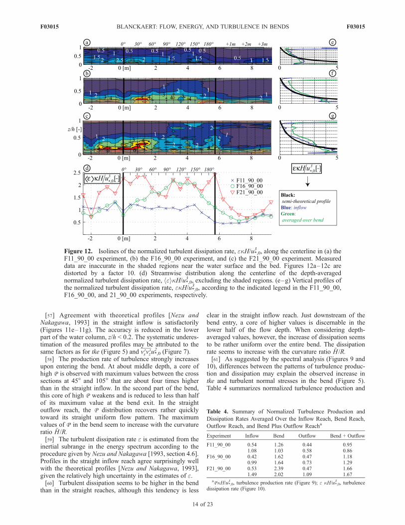
upon entering the bend. At about middle depth, a core ofhigh P is observed with maximum values between the crosssections at 45� and 105� that are about four times higherthan in the straight inflow. In the second part of the bend,this core of high P weakens and is reduced to less than halfof its maximum value at the bend exit. In the straightoutflow reach, the P distribution recovers rather quicklytoward its straight uniform flow pattern. The maximumvalues of P in the bend seem to increase with the curvatureratio ~H /R.[59] The turbulent dissipation rate e is estimated from the

inertial subrange in the energy spectrum according to theprocedure given by Nezu and Nakagawa [1993, section 4.6].Profiles in the straight inflow reach agree surprisingly wellwith the theoretical profiles [Nezu and Nakagawa, 1993],given the relatively high uncertainty in the estimates of e.[60] Turbulent dissipation seems to be higher in the bend

than in the straight reaches, although this tendency is less

clear in the straight inflow reach. Just downstream of thebend entry, a core of higher values is discernable in thelower half of the flow depth. When considering depth-averaged values, however, the increase of dissipation seemsto be rather uniform over the entire bend. The dissipationrate seems to increase with the curvature ratio ~H /R.[61] As suggested by the spectral analysis (Figures 9 and

10), differences between the patterns of turbulence produc-tion and dissipation may explain the observed increase intke and turbulent normal stresses in the bend (Figure 5).Table 4 summarizes normalized turbulence production and

Figure 12. Isolines of the normalized turbulent dissipation rate, ekH/u*,03 , along the centerline in (a) the

F11_90_00 experiment, (b) the F16_90_00 experiment, and (c) the F21_90_00 experiment. Measureddata are inaccurate in the shaded regions near the water surface and the bed. Figures 12a–12c aredistorted by a factor 10. (d) Streamwise distribution along the centerline of the depth-averagednormalized turbulent dissipation rate, heikH/u*,03 , excluding the shaded regions. (e–g) Vertical profiles ofthe normalized turbulent dissipation rate, ekH/u*,0

3 , according to the indicated legend in the F11_90_00,F16_90_00, and 21_90_00 experiments, respectively.

Table 4. Summary of Normalized Turbulence Production and

Dissipation Rates Averaged Over the Inflow Reach, Bend Reach,

Outflow Reach, and Bend Plus Outflow Reacha

Experiment Inflow Bend Outflow Bend + Outflow

F11_90_00 0.54 1.26 0.44 0.951.08 1.03 0.58 0.86

F16_90_00 0.42 1.62 0.47 1.180.99 1.64 0.73 1.29

F21_90_00 0.53 2.39 0.47 1.661.49 2.02 1.09 1.67

aPkH/u*,03 , turbulence production rate (Figure 9); e kH/u*,0

3 , turbulencedissipation rate (Figure 10).


14 of 23

F03015

dissipation rates, P kH/u*,03 (Figure 11) and ekH/u*,0

3

(Figure 12), respectively (k = 0.4 is the von Karmanconstant), averaged over the inflow reach, bend reach,outflow reach and bend plus outflow reach. The experi-mental uncertainties in the turbulence production and dis-sipation rates are inherently high and have been estimatedat 50% and 100%, respectively. Moreover, measurementsof turbulence production and dissipation rates are system-atically underestimated in the near bed region where thesevariables attain their highest values (Figures 11e–11g andFigures 12e–12g, respectively), leading to systematic under-estimations of the averaged values reported in Table 4.These high experimental uncertainties and systematic errorsmake the following data interpretation unavoidably some-what tentative:[62] 1. Dissipation seems to be considerably overesti-

mated in the straight inflow reach, where it should theoret-ically be equal to production. It is not clear if thesedeviations are uniquely due to the experimental uncertaintyor if they have a physical basis.[63] 2. When excluding the straight inflow reach, how-

ever, the total production and dissipation differ by less than10% and can be considered in equilibrium.[64] 3. Turbulence production seems to react faster to

changes in curvature than turbulent dissipation: its growth ismore pronounced in the first part of the bend, it reacheshigher maximum values, and it recovers faster toward‘‘straight flow’’ patterns in the straight outflow reach. Theslower adaptation of the turbulent dissipation seems toattenuate spatial variations. This different behavior of theproduction and dissipation rate of tke is in agreement withthe concept of the turbulent energy cascade as aforemen-tioned in the spectral analysis.

[65] 4. Averaged over the bend, production seems to behigher than dissipation, which is compensated by the higherdissipation in the straight outflow reach.[66] 5. The increase of tke and turbulent normal stresses

can be attributed to these different spatial distributions ofthe turbulent production and dissipation. Turbulent produc-tion shows more spatial variation than dissipation andreaches considerably higher peak values. The regions wherethe peak values in production occur correspond rather wellwith the region of maximum tke and turbulent normalstresses.[67] The relation between spatial differences in produc-

tion and dissipation rate of turbulence at the one hand andthe increase in tke at the other can be quantified by means ofthe transport equation for depth-averaged tke [Hinze, 1975]reduced to its three principal terms:

U@hki@s

¼ hP i � hei ð8Þ

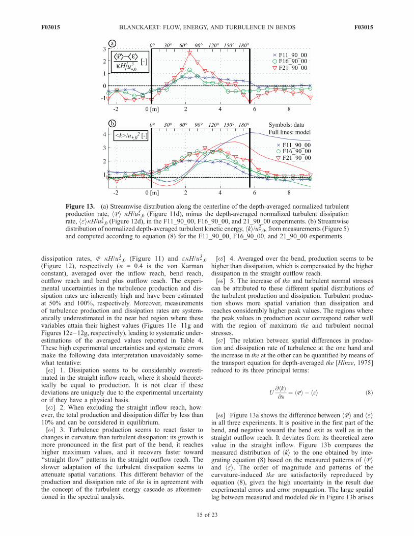
[68] Figure 13a shows the difference between hP i and heiin all three experiments. It is positive in the first part of thebend, and negative toward the bend exit as well as in thestraight outflow reach. It deviates from its theoretical zerovalue in the straight inflow. Figure 13b compares themeasured distribution of hki to the one obtained by inte-grating equation (8) based on the measured patterns of hP iand hei. The order of magnitude and patterns of thecurvature-induced tke are satisfactorily reproduced byequation (8), given the high uncertainty in the result dueexperimental errors and error propagation. The large spatiallag between measured and modeled tke in Figure 13b arises

Figure 13. (a) Streamwise distribution along the centerline of the depth-averaged normalized turbulentproduction rate, hP i kH/u*,0

3 (Figure 11d), minus the depth-averaged normalized turbulent dissipationrate, heikH/u*,03 (Figure 12d), in the F11_90_00, F16_90_00, and 21_90_00 experiments. (b) Streamwisedistribution of normalized depth-averaged turbulent kinetic energy, hki/u*,02 , from measurements (Figure 5)and computed according to equation (8) for the F11_90_00, F16_90_00, and 21_90_00 experiments.


15 of 23

F03015

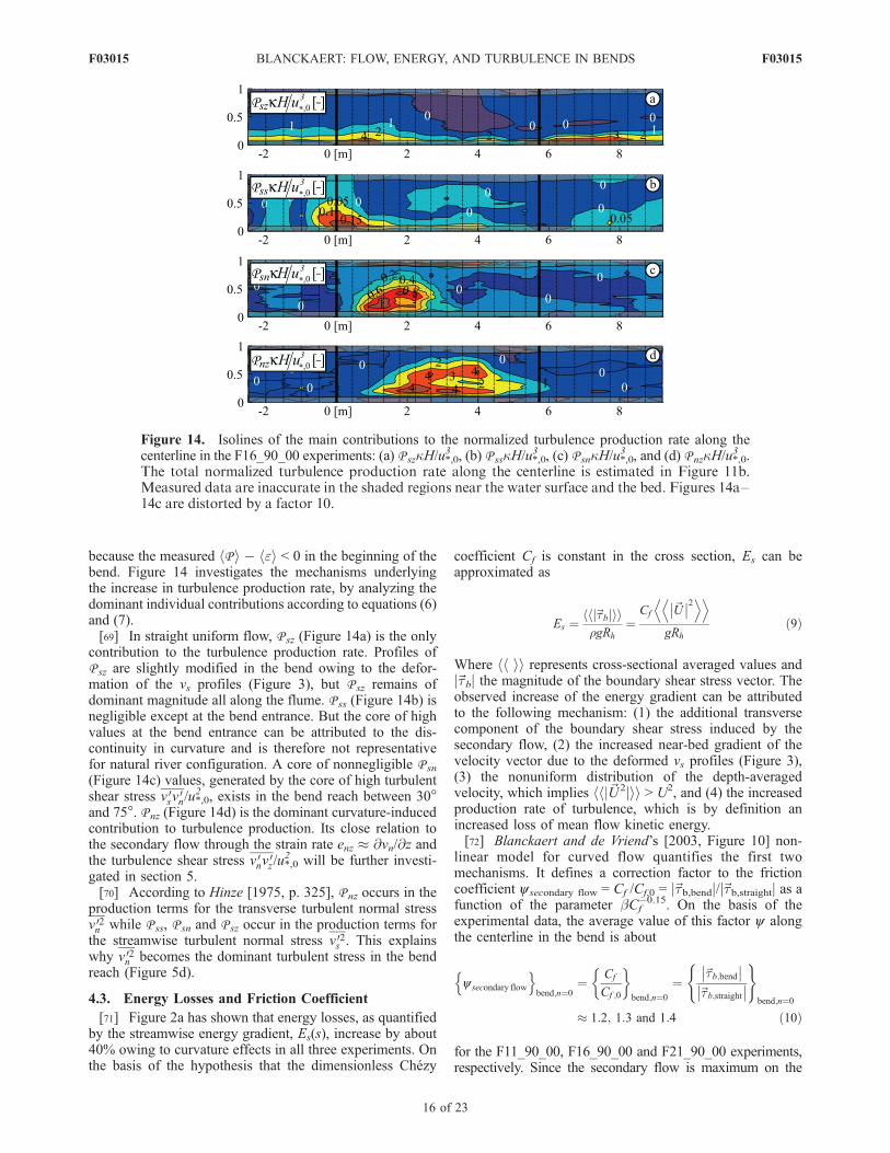
because the measured hP i � hei < 0 in the beginning of thebend. Figure 14 investigates the mechanisms underlyingthe increase in turbulence production rate, by analyzing thedominant individual contributions according to equations (6)and (7).[69] In straight uniform flow, P sz (Figure 14a) is the only

contribution to the turbulence production rate. Profiles ofP sz are slightly modified in the bend owing to the defor-mation of the vs profiles (Figure 3), but P sz remains ofdominant magnitude all along the flume. P ss (Figure 14b) isnegligible except at the bend entrance. But the core of highvalues at the bend entrance can be attributed to the dis-continuity in curvature and is therefore not representativefor natural river configuration. A core of nonnegligible P sn

(Figure 14c) values, generated by the core of high turbulentshear stress v 0sv

0n/u*,0

2 , exists in the bend reach between 30�and 75�. P nz (Figure 14d) is the dominant curvature-inducedcontribution to turbulence production. Its close relation tothe secondary flow through the strain rate enz � @vn/@z andthe turbulence shear stress v 0nv

0z/u*,0

2 will be further investi-gated in section 5.[70] According to Hinze [1975, p. 325], P nz occurs in the

production terms for the transverse turbulent normal stressv 02n while P ss, P sn and P sz occur in the production terms forthe streamwise turbulent normal stress v 02s . This explainswhy v 02n becomes the dominant turbulent stress in the bendreach (Figure 5d).

4.3. Energy Losses and Friction Coefficient

[71] Figure 2a has shown that energy losses, as quantifiedby the streamwise energy gradient, Es(s), increase by about40% owing to curvature effects in all three experiments. Onthe basis of the hypothesis that the dimensionless Chezy

coefficient Cf is constant in the cross section, Es can beapproximated as

Es ¼~tbj jh ih irgRh

¼Cf

~U�� 2D ED EgRh

ð9Þ

Where hh ii represents cross-sectional averaged values andj~tbj the magnitude of the boundary shear stress vector. Theobserved increase of the energy gradient can be attributedto the following mechanism: (1) the additional transversecomponent of the boundary shear stress induced by thesecondary flow, (2) the increased near-bed gradient of thevelocity vector due to the deformed vs profiles (Figure 3),(3) the nonuniform distribution of the depth-averagedvelocity, which implies hhj~U2jii > U2, and (4) the increasedproduction rate of turbulence, which is by definition anincreased loss of mean flow kinetic energy.[72] Blanckaert and de Vriend’s [2003, Figure 10] non-

linear model for curved flow quantifies the first twomechanisms. It defines a correction factor to the frictioncoefficient ysecondary flow = Cf /Cf,0 = j~tb,bendj/j~tb,straightj as afunction of the parameter bCf

�0.15. On the basis of theexperimental data, the average value of this factor y alongthe centerline in the bend is about

ysecondary flow

n obend;n¼0

¼ Cf

Cf ;0

� �bend;n¼0

¼~tb;bend�� ~tb;straight��

( )bend;n¼0

� 1:2; 1:3 and 1:4 ð10Þ

for the F11_90_00, F16_90_00 and F21_90_00 experiments,respectively. Since the secondary flow is maximum on the

Figure 14. Isolines of the main contributions to the normalized turbulence production rate along thecenterline in the F16_90_00 experiments: (a) P szkH/u*,0

3 , (b) P sskH/u*,03 , (c) P snkH/u*,0

3 , and (d) P nzkH/u*,03 .

The total normalized turbulence production rate along the centerline is estimated in Figure 11b.Measured data are inaccurate in the shaded regions near the water surface and the bed. Figures 14a–14c are distorted by a factor 10.


16 of 23

F03015

centerline, the bend averaged value ofysecondary flow is expectedto be lower than the average value along the centerline.[73] The relevance of the third mechanism can be esti-

mated on the basis of a linearization of the velocitydistribution according to equation (3): Ulinear(s, n) =U(s)(1 + as(s)n/R). Averaging over the cross section (theaverage is in fact taken over a bend sector in order to takeinto account that arc length is longer/shorter in the outer/inner part of the cross section than on the centerline), gives

yas¼

~U�� 2D ED EU2

¼ 1þ 1

12a2s þ 2as

� �B2

R2ð11Þ

This effect can only cause a relevant increase in energygradient of maximum 50% in very sharp bends where amobile bed topography causes high as values. In the threereported experiments, however, the negative as values in alarge part of the bend cause a negligible bend-averageddecrease in energy gradient.[74] These observations suggest that the increased produc-

tion rate of tke in the bend of O(100%) (Table 4) is amechanism of dominant order of magnitude in the experi-ments. This mechanism will be further analyzed in section 5.

5. Modeling Implications

[75] As aforementioned, the nonlinear model ofBlanckaert and de Vriend [2003] is able to explain theinteraction between vertical profiles of the streamwisevelocity vs and the secondary flow, (vn � Un). This sectionwill focus on the modeling of the curvature-induced in-crease in tke and in energy losses.[76] According to section 4, the spatial distribution of the

production rate of turbulence P (Figure 11) is a dominantmechanism with respect to the curvature-induced increase inenergy losses and tke (Figure 5). The model proposedhereafter for curvature-induced increase in energy lossesand tke will be based on a model for the curvature-inducedincrease in turbulence production rate P .[77] The production rate of turbulence in straight uniform

flow P straight is theoretically known as [Nezu and Nakagawa,1993]

P straight ¼ P sz ¼ �2v 0sv0zesz ¼ 4nte2sz ¼

u3�;0kh

1� z=h

z=h

� �ð12Þ

P bend will be approximated on the basis of its majorcontributions as (equations (5), (6), (7))

P bend � P ss þ P sn þ P sz þ P nz

¼ � v 02s � 2

3k

� �ess þ 2v 0sv

0nesn þ 2v 0sv

0zesz þ 2v 0nv

0zenz

� ð13Þ

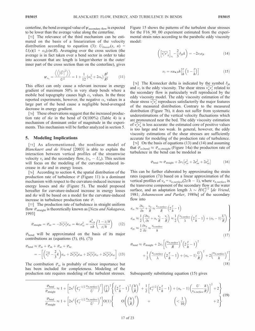
The contribution P ss is probably of minor importance buthas been included for completeness. Modeling of theproduction rate requires modeling of the turbulent stresses.

Figure 15 shows the patterns of the turbulent shear stressesfor the F16_90_00 experiment estimated from the experi-mental strain rates according to the parabolic eddy viscositymodel:

v 0j v0k

h int� 2

3djk k

� �¼ �2ntejk ð14Þ

nt ¼ ku*;0hz

h1� z

h

� �h ið15Þ

[78] The Kronecker delta is indicated by the symbol djkand nt is the eddy viscosity. The shear stress v 0nv

0z related to

the secondary flow is particularly well reproduced by theeddy viscosity model. The eddy viscosity estimation of theshear stress v 0sv

0z reproduces satisfactorily the major features

of the measured distribution. Contrary to the measureddistribution (Figure 7b), it does not suffer from systematicunderestimations of the vertical velocity fluctuations whichare pronounced near the bed. The eddy viscosity estimationof v 0sv

0n is less accurate: the estimated core of positive values

is too large and too weak. In general, however, the eddyviscosity estimations of the shear stresses are sufficientlyaccurate for modeling of the production rate of turbulence.[79] On the basis of equations (13) and (14) and assuming

that P sz,bend � P sz,straight (Figure 14a) the production rate ofturbulence in the bend can be modeled as

P bend � P straight þ 2nt e2ss þ 2e2sn þ 2e2nz� �

ð16Þ

This can be further elaborated by approximating the strainrates (equation (7)) based on a linear approximation of thevertical profiles of vn = vn,surface(2z/h � 1), where vn,surface isthe transverse component of the secondary flow at the watersurface, and an adaptation length l � H/Cf

1/2 [de Vriend,1981; Johannesson and Parker, 1989a] of the secondaryflow into

ess �@vs@s

þ vn

R� vn;surface

R2z

h� 1

� �

esn �1

2

@vn@s

þ as

vs

R� vs

R

� �� 1

2

vn;surface

l2z

h� 1

� �þ as � 1ð ÞU

R

� �

enz �1

2

@vn@z

� vn;surface

h

9>>>>>>=>>>>>>;

ð17Þ

P bend � P straight þ 2nt

�vn;surface

R

� �22z

h� 1

� �2

þ 1

2

vn;surface

l2z

h� 1

� �þ as � 1ð ÞU

R

� �2

þ 2vn;surface

h

� �2ð18Þ

Subsequently substituting equation (15) gives

P bend

P straight

� 1þ 2k2 C�1=2f

vn;surface

U

� �2� z

h

� �22z

h� 1

� �2 h

R

� �2

þ 1

2C

1=2f 2

z

h� 1

� �þ as � 1ð Þ U

vn;surface

h

R

� �� 2þ 2

( )

P bend

P straight

� 1þ 2k2 C�1=2f

vn;surface

U

� �2� Oð1Þ O

h

R

� �2 !

þ <1

10

� �þ 2

( ) (19)


17 of 23

F03015

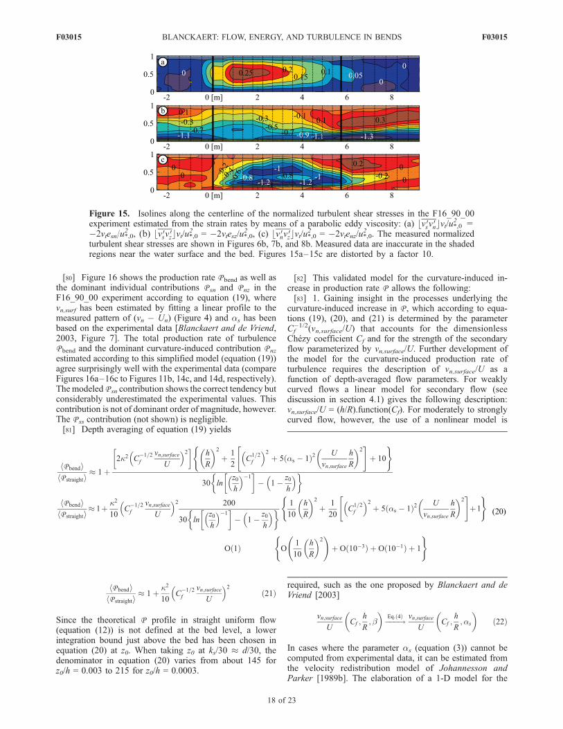
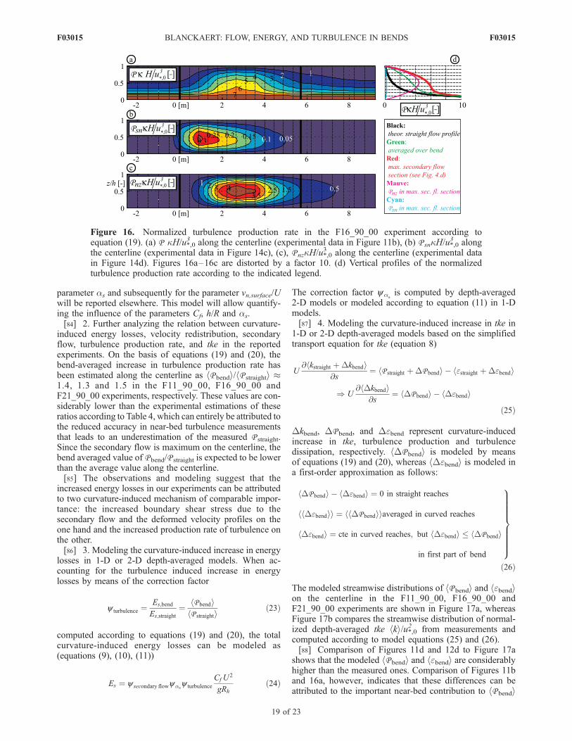
[80] Figure 16 shows the production rate P bend as well asthe dominant individual contributions P sn and P nz in theF16_90_00 experiment according to equation (19), wherevn,surf has been estimated by fitting a linear profile to themeasured pattern of (vn � Un) (Figure 4) and as has beenbased on the experimental data [Blanckaert and de Vriend,2003, Figure 7]. The total production rate of turbulenceP bend and the dominant curvature-induced contribution P nz

estimated according to this simplified model (equation (19))agree surprisingly well with the experimental data (compareFigures 16a–16c to Figures 11b, 14c, and 14d, respectively).The modeled P sn contribution shows the correct tendency butconsiderably underestimated the experimental values. Thiscontribution is not of dominant order of magnitude, however.The P ss contribution (not shown) is negligible.[81] Depth averaging of equation (19) yields

hP bendihP straighti

� 1þ2k2 C

�1=2f

vn;surface

U

� �2� h

R

� �2

þ 1

2C

1=2f

� �2þ 5 as � 1ð Þ2 U

vn;surface

h

R

� �2" #

þ 10

( )

30 lnz0

h

� ��1�

� 1� z0

h

� ��


� 1þ k2

10C

�1=2f

vn;surface

U

� �2 200

30 lnz0

h

� ��1�

� 1� z0

h

� �� 1

10

h

R

� �2

þ 1

20C

1=2f

� �2þ 5 as � 1ð Þ2 U

vn;surface

h

R

� �2" #

þ1

( )

Oð1Þ O1

10

h

R

� �2 !

þ Oð10�3Þ þ Oð10�1Þ þ 1

( )


� 1þ k2

10C

�1=2f

vn;surface

U

� �2ð21Þ

Since the theoretical P profile in straight uniform flow(equation (12)) is not defined at the bed level, a lowerintegration bound just above the bed has been chosen inequation (20) at z0. When taking z0 at ks/30 � d/30, thedenominator in equation (20) varies from about 145 forz0/h = 0.003 to 215 for z0/h = 0.0003.

[82] This validated model for the curvature-induced in-crease in production rate P allows the following:[83] 1. Gaining insight in the processes underlying the

curvature-induced increase in P , which according to equa-tions (19), (20), and (21) is determined by the parameterCf�1/2(vn,surface/U) that accounts for the dimensionless

Chezy coefficient Cf and for the strength of the secondaryflow parameterized by vn,surface/U. Further development ofthe model for the curvature-induced production rate ofturbulence requires the description of vn,surface/U as afunction of depth-averaged flow parameters. For weaklycurved flows a linear model for secondary flow (seediscussion in section 4.1) gives the following description:vn,surface/U = (h/R).function(Cf). For moderately to stronglycurved flow, however, the use of a nonlinear model is

required, such as the one proposed by Blanckaert and deVriend [2003]

vn;surface

UCf ;

h

R; b

� ��!Eq:ð4Þ vn;surface

UCf ;

h

R;as

� �ð22Þ

In cases where the parameter as (equation (3)) cannot becomputed from experimental data, it can be estimated fromthe velocity redistribution model of Johannesson andParker [1989b]. The elaboration of a 1-D model for the

Figure 15. Isolines along the centerline of the normalized turbulent shear stresses in the F16_90_00experiment estimated from the strain rates by means of a parabolic eddy viscosity: (a) bv 0sv 0ncvt/u*,0

2 =�2vtesn/u*,0

2 , (b) bv 0sv 0zcvt/u*,02 = �2vtesz/u*,0

2 , (c) bv 0nv 0zcvt/u*,02 = �2vtenz/u*,0

2 . The measured normalizedturbulent shear stresses are shown in Figures 6b, 7b, and 8b. Measured data are inaccurate in the shadedregions near the water surface and the bed. Figures 15a–15c are distorted by a factor 10.

(20)


18 of 23

F03015

parameter as and subsequently for the parameter vn,surface/Uwill be reported elsewhere. This model will allow quantify-ing the influence of the parameters Cf, h/R and as.[84] 2. Further analyzing the relation between curvature-

induced energy losses, velocity redistribution, secondaryflow, turbulence production rate, and tke in the reportedexperiments. On the basis of equations (19) and (20), thebend-averaged increase in turbulence production rate hasbeen estimated along the centerline as hP bendi/hP straighti �1.4, 1.3 and 1.5 in the F11_90_00, F16_90_00 andF21_90_00 experiments, respectively. These values are con-siderably lower than the experimental estimations of theseratios according to Table 4, which can entirely be attributed tothe reduced accuracy in near-bed turbulence measurementsthat leads to an underestimation of the measured P straight.Since the secondary flow is maximum on the centerline, thebend averaged value of P bend/P straight is expected to be lowerthan the average value along the centerline.[85] The observations and modeling suggest that the

increased energy losses in our experiments can be attributedto two curvature-induced mechanism of comparable impor-tance: the increased boundary shear stress due to thesecondary flow and the deformed velocity profiles on theone hand and the increased production rate of turbulence onthe other.[86] 3. Modeling the curvature-induced increase in energy

losses in 1-D or 2-D depth-averaged models. When ac-counting for the turbulence induced increase in energylosses by means of the correction factor

y turbulence ¼Es;bend

Es;straight¼ hP bendi

hP straightið23Þ

computed according to equations (19) and (20), the totalcurvature-induced energy losses can be modeled as(equations (9), (10), (11))

Es ¼ ysecondary flowyasy turbulence

Cf U2

gRh

ð24Þ

The correction factor yasis computed by depth-averaged

2-D models or modeled according to equation (11) in 1-Dmodels.[87] 4. Modeling the curvature-induced increase in tke in

1-D or 2-D depth-averaged models based on the simplifiedtransport equation for tke (equation 8)

U@hkstraight þDkbendi

@s¼ hP straight þDP bendi � hestraight þDebendi

) U@hDkbendi

@s¼ hDP bendi � hDebendi

ð25Þ

Dkbend, DP bend, and Debend represent curvature-inducedincrease in tke, turbulence production and turbulencedissipation, respectively. hDP bendi is modeled by meansof equations (19) and (20), whereas hDebendi is modeled ina first-order approximation as follows:

hDP bendi � hDebendi ¼ 0 in straight reaches

hhDebendii ¼ hhDP bendiiaveraged in curved reaches

hDebendi ¼ cte in curved reaches; but hDebendi � hDP bendi

in first part of bend

9>>>>>>>>=>>>>>>>>;ð26Þ

The modeled streamwise distributions of hP bendi and hebendion the centerline in the F11_90_00, F16_90_00 andF21_90_00 experiments are shown in Figure 17a, whereasFigure 17b compares the streamwise distribution of normal-ized depth-averaged tke hki/u*,02 from measurements andcomputed according to model equations (25) and (26).[88] Comparison of Figures 11d and 12d to Figure 17a

shows that the modeled hP bendi and hebendi are considerablyhigher than the measured ones. Comparison of Figures 11band 16a, however, indicates that these differences can beattributed to the important near-bed contribution to hP bendi

Figure 16. Normalized turbulence production rate in the F16_90_00 experiment according toequation (19). (a) P kH/u*,0

3 along the centerline (experimental data in Figure 11b), (b) P snkH/u*,03 along

the centerline (experimental data in Figure 14c), (c), P nzkH/u*,03 along the centerline (experimental data

in Figure 14d). Figures 16a–16c are distorted by a factor 10. (d) Vertical profiles of the normalizedturbulence production rate according to the indicated legend.


19 of 23

F03015

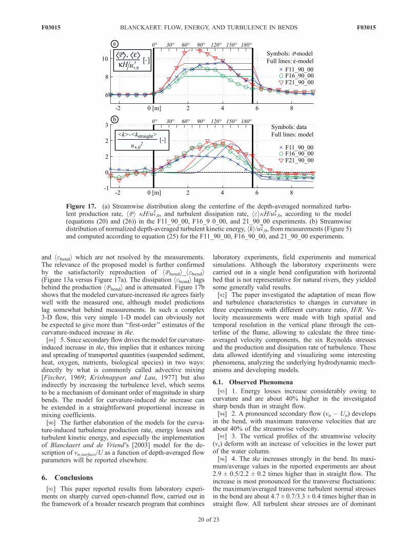
and hebendi which are not resolved by the measurements.The relevance of the proposed model is further confirmedby the satisfactorily reproduction of hP bendi_hebendi(Figure 13a versus Figure 17a). The dissipation hebendi lagsbehind the production hP bendi and is attenuated. Figure 17bshows that the modeled curvature-increased tke agrees fairlywell with the measured one, although model predictionslag somewhat behind measurements. In such a complex3-D flow, this very simple 1-D model can obviously notbe expected to give more than ‘‘first-order’’ estimates of thecurvature-induced increase in tke.[89] 5. Since secondary flow drives the model for curvature-

induced increase in tke, this implies that it enhances mixingand spreading of transported quantities (suspended sediment,heat, oxygen, nutrients, biological species) in two ways:directly by what is commonly called advective mixing[Fischer, 1969; Krishnappan and Lau, 1977] but alsoindirectly by increasing the turbulence level, which seemsto be a mechanism of dominant order of magnitude in sharpbends. The model for curvature-induced tke increase canbe extended in a straightforward proportional increase inmixing coefficients.[90] The further elaboration of the models for the curva-

ture-induced turbulence production rate, energy losses andturbulent kinetic energy, and especially the implementationof Blanckaert and de Vriend’s [2003] model for the de-scription of vn,surface/U as a function of depth-averaged flowparameters will be reported elsewhere.

6. Conclusions

[91] This paper reported results from laboratory experi-ments on sharply curved open-channel flow, carried out inthe framework of a broader research program that combines

laboratory experiments, field experiments and numericalsimulations. Although the laboratory experiments werecarried out in a single bend configuration with horizontalbed that is not representative for natural rivers, they yieldedsome generally valid results.[92] The paper investigated the adaptation of mean flow

and turbulence characteristics to changes in curvature inthree experiments with different curvature ratio, H/R. Ve-locity measurements were made with high spatial andtemporal resolution in the vertical plane through the cen-terline of the flume, allowing to calculate the three time-averaged velocity components, the six Reynolds stressesand the production and dissipation rate of turbulence. Thesedata allowed identifying and visualizing some interestingphenomena, analyzing the underlying hydrodynamic mech-anisms and developing models.

6.1. Observed Phenomena

[93] 1. Energy losses increase considerably owing tocurvature and are about 40% higher in the investigatedsharp bends than in straight flow.[94] 2. A pronounced secondary flow (vn � Un) develops

in the bend, with maximum transverse velocities that areabout 40% of the streamwise velocity.[95] 3. The vertical profiles of the streamwise velocity

(vs) deform with an increase of velocities in the lower partof the water column.[96] 4. The tke increases strongly in the bend. Its maxi-

mum/average values in the reported experiments are about2.9 ± 0.5/2.2 ± 0.2 times higher than in straight flow. Theincrease is most pronounced for the transverse fluctuations:the maximum/averaged transverse turbulent normal stressesin the bend are about 4.7 ± 0.7/3.3 ± 0.4 times higher than instraight flow. All turbulent shear stresses are of dominant

Figure 17. (a) Streamwise distribution along the centerline of the depth-averaged normalized turbu-lent production rate, hP i kH/u*,0

3 , and turbulent dissipation rate, heikH/u*,03 , according to the model(equations (20) and (26)) in the F11_90_00, F16_9 0_00, and 21_90_00 experiments. (b) Streamwisedistribution of normalized depth-averaged turbulent kinetic energy, hki/u*,02 , from measurements (Figure 5)and computed according to equation (25) for the F11_90_00, F16_90_00, and 21_90_00 experiments.


20 of 23

F03015

order of magnitude in the bend. This curvature-inducedincrease in turbulence is relevant with respect to spreadingand mixing of suspended matter, oxygen or nutrients,temperature, to sediment transport and scour.[97] 5. The secondary flow, energy losses, and turbulence

do not increase proportionally to the curvature ratio H/R, ascould be expected on the basis of a linear perturbationapproach. The secondary flow and the energy losses areabout identical in the three experiments, and the turbulencecharacteristics only seem to increase weakly. These obser-vations indicate a saturation of curvature effects in verysharply curved open-channel flow.[98] 6. The recovery length toward straight flow hydro-

dynamic characteristics seems to increase with the flowdepth H.

6.2. Underlying Flow Mechanisms

[99] 1. Blanckaert and Graf [2004] and Blanckaert andde Vriend [2003] have analyzed and explained the interac-tion and feedback between streamwise and cross-streamvelocities. Advective momentum transport by the secondaryflow deforms the vs profiles, which reduces the drivingmechanism of the secondary flow. This nonlinear feedbackbetween vs and (vn � Un) ultimately leads to the observedsaturation of the secondary flow for very sharp curvatures.[100] 2. The analysis of spectral dynamics and of stream-

wise patterns of turbulence production and dissipation ratessuggests the following mechanism underlying curvature-induced increased turbulence. Production and dissipationrates are considerably increased by curvature effects. Theyare about in equilibrium averaged over the bend, but havedifferent spatial distributions. Production is considerablylarger/smaller than dissipation in the first/second half of thebend, leading to an increase/decrease of turbulent kineticenergy. This lagging of the dissipation rate behind theproduction rate is in line with the energy cascade concept ofturbulence. The production rate of turbulence is dominated bythe contribution due to the cross-sectional turbulence shearstress v 0nv

0z which is closely related to the secondary flow.

[101] 3. The increased energy losses in the bend can beattributed to four mechanisms: (1) the additional transversecomponent of the boundary shear stress induced by thesecondary flow, (2) the increased near-bed gradient of thevelocity vector due to the deformed vs profiles (Figure 3),(3) the increased production rate of turbulence, (4) thenonuniform distribution of the depth-averaged velocity. Inthe reported experiments, mechanisms 1 and 2 on the onehand and 3 on the other hand were found to be dominantand of comparable magnitude, whereas mechanism 4 wasfound to be negligible.[102] It can be concluded that the curvature-induced

secondary flow is the dominant mechanism in the reportedexperiments: it is directly or indirectly responsible for thedeformation of the vs profiles, the curvature-induced in-creased turbulence production rate, turbulent stresses, tkeand energy losses. The role of curvature-induced secondaryflow is accentuated in the investigated laboratory config-urations with rectangular cross section. In sharply curvedreal rivers, the mobile bed bathymetry is expected to havealso an influence of dominant order of magnitude on thecharacteristics of the turbulence production rate, turbulentstresses, tke and energy losses.

6.3. Modeling Implications

[103] 1. Blanckaert and de Vriend [2003] have reported amodel for the vs and (vn � Un) profiles that accounts fortheir nonlinear interaction and includes the saturation of thesecondary flow in very sharply curved open-channel flow.This model can parameterize curvature effects in 1-D ordepth-averaged 2-D hydrodynamic models.[104] 2. The eddy viscosity concept is shown to represent

satisfactorily the turbulent shear stresses, and especially thedominant cross-stream turbulent shear stress v 0nv

0z which is

closely related to the secondary flow.[105] 3. On the basis of the eddy viscosity concept and a

parameterization of the profiles of streamwise velocity andsecondary flow, a model for the curvature-induced increasein turbulence production rate has been developed andvalidated by means of the reported experimental data. Thismodel quantifies the influence of different geometric andhydraulic parameters and identifies (Cf

�1/2vn,surf /U) as thedominant scaling parameter.[106] 4. Correction factors to the friction factor that

parameterize curvature-induced increase in energy losseshave been derived. They account for curvature-inducedturbulence production rate, secondary flow and the nonuni-formity of the velocity distribution.[107] 5. On the basis of the model for curvature-induced

increase in turbulence production rate, a 1-D model isdeveloped for the curvature-induced increase in tke andmixing.[108] Owing to limitations in computational capacity,

long-term (scale of a flood event to geological scales) orlarge-scale (scale of a river basin) investigations make useof 1-D or 2-D depth-averaged morphodynamic models. Asaforementioned, such models are currently unable to de-scribe curvature-induced turbulence and energy losses, andthey are limited to a simplified parameterization of the time-averaged flow based on a model for secondary flow whichvalidity is limited to low and moderate curvatures. The herereported results allow enhancing existing 1-D or 2-D depth-averaged morphodynamic models by extending the validityrange to sharp curvatures and by including a parameteriza-tion for curvature-induced increase in energy losses, tke andmixing. These extensions may improve the models’ predic-tive capacity and reliability in multiple applications. Abetter understanding and modeling of the investigatedprocesses may lead to more accurate estimations of theboundary shear stress, the sediment transport, the convey-ance capacity and the water quality, a better assessment ofnatural hazards and the development of less expensive andmore environmentally friendly bank protection measures aswell as river restoration schemes that can guarantee theconservation of biodiversity. The extension of the validityrange to sharp curvatures is important with respect tomeander dynamics, and especially with respect to themodeling of cutoff events and the accompanying localrestraightening. The frequency of occurrence of these eventsdetermines the rate of floodplain rejuvenation as well as thesedimentologic structure of the meander belt. The former isan important ecological parameter, whereas knowledge ofthe latter is required for the sustainable exploitation ofdrinking water of hydrocarburates.[109] Beside enhancing insight in the hydrodynamics of

sharply curved open-channel flow and improving modeling


21 of 23

F03015

tools, the reported data are useful for the validation ofnumerical codes. More data from the reported experimentsand from other experiments (Blanckaert, submitted manu-script, 2009) can be obtained from the author.

[110] Acknowledgments. This research was supported by the SwissNational Science Foundation under grants 2100-052257.97 and 2000-059392.99 and by the Netherlands Organization for Scientific Research(NWO) under grant DN66-149. The author wishes to acknowledge W. H.Graf, H. J. de Vriend, and W. S. J. Uijttewaal as well as R. Ferguson,A. Sukhodolov, M. Garcia, and an anonymous reviewer for constructivecomments that improved the manuscript.

ReferencesAndrle, R. (1994), Flow structure and development of circular meanderpools, Geomorphology, 9, 261 – 270, doi:10.1016/0169-555X(94)90049-3.

Argawal, V. C., R. J. Garde, and K. G. Ranga Raju (1984), Resistance toflow and sediment transport in curved alluvial channels, paper presentedat 4th Congress, IAHR- APD, Chiang Mai, Thailand.

Bagnold, R. A. (1960), Some aspects of the shape of river meanders, U.S.Geol. Surv. Prof. Pap., 282E135–144.

Batchelor, G. K. (1967), An Introduction to Fluid Dynamics, CambridgeUniv. Press, Cambridge, U. K.

Bathurst, J. C., C. R. Thorne, and R. D. Hey (1979), Secondary flow andshear stress at river bends, J. Hydraul. Div. Am. Soc. Civ. Eng., 105(10),1277–1295.

Biedenharn, D. S., P. G. Combs, G. J. Hill, C. F. J. Pinkard, and C. B.Pinkston (1989), Relation between channel migration and radius of cur-vature on the Red river, in Sediment Transport Modeling: Proceedings ofthe International Symposium, edited by S. Y. Sam Wang, pp. 536–541,Am. Soc. of Civ. Eng., New York.

Blanckaert, K., and H. J. de Vriend (2003), Nonlinear modeling of meanflow redistribution in curved open channels, Water Resour. Res., 39(12),1375, doi:10.1029/2003WR002068.

Blanckaert, K., and H. J. de Vriend (2004), Secondary flow in sharpopen-channel bends, J. Fluid Mech., 498, 353 –380, doi:10.1017/S0022112003006979.

Blanckaert, K., and W. H. Graf (2001), Experiments on flow in an open-channel bend: Mean flow and turbulence, J. Hydraul. Eng., 127(10),835–847, doi:10.1061/(ASCE)0733-9429(2001)127:10(835).

Blanckaert, K., and W. H. Graf (2004), Momentum transport in sharp open-channel bends, J. Hydraul. Eng., 130(3), 186 – 198, doi:10.1061/(ASCE)0733-9429(2004)130:3(186).

Blanckaert, K., and U. Lemmin (2006), Means of noise reduction in acous-tic turbulence measurements, J. Hydraul. Res., 44(1), 3–17.

Crosato, A. (2008), Analysis and modelling of river meandering, Ph.D.thesis, Delft Univ. of Technol., Delft, Netherlands.

de Vriend, H. J. (1977), A mathematical model of steady flow in curvedshallow channels, J. Hydraul. Res., 15(1), 37–54.

de Vriend, H. J. (1981), Steady flow in shallow channel bends, Rep. 81–3,Fluid Mech. Lab., Dept. of Civ. Eng., Delft Univ. of Technol, Delft,Netherlands.

Edwards, B. F., and D. H. Smith (2002), River meandering dynamics, Phys.Rev. E, 65, 1–12.

Engelund, F. (1974), Flow and bed topography in channel bends, J. Hydraul.Div. Am. Soc. Civ. Eng., 100(HY11), 1631–1648.

Ferguson, R. I., D. R. Parsons, S. N. Lane, and R. J. Hardy (2003), Flow inmeander bends with recirculation at the inner bank, Water Resour. Res.,39(11), 1322, doi:10.1029/2003WR001965.

Fischer, H. B. (1969), Effects of bends on dispersion in streams, WaterResour. Res., 5, 496–506, doi:10.1029/WR005i002p00496.

Furbish, D. J. (1988), River-bend curvature and migration: How are theyrelated?, Geology, 16(8), 752 – 755, doi:10.1130/0091-7613(1988)016<0752:RBCAMH>2.3.CO;2.

Graf, W. H., and M. Altinakar (1998), Fluvial Hydraulics: Flow and Trans-port Processes in Channels of Simple Geometry, John Wiley, Chichester,U. K.

Hickin, E. J. (1974), The development of meanders in natural river-channels,Am. J. Sci., 274, 414–442.

Hickin, E. J., and G. C. Nanson (1975), The character of channel migrationon the Beatton river, northeast British Columbia, Canada, Geol. Soc. Am.Bull., 86, 487–494, doi:10.1130/0016-7606(1975)86<487:TCOCMO>2.0.CO;2.

Hinze, J. O. (1975), Turbulence, McGraw-Hill, New York.Hooke, J. M. (1987), Changes in meander morphology, in InternationalGeomorphology 1986 Part I, edited by V. Gardiner, pp. 591–609, JohnWiley, Chichester, U. K.

Hurther, D., and U. Lemmin (1998), A constant beamwidth transducer forthree-dimensional Doppler profile measurements in open channel flow,Meas. Sci. Technol., 9(10), 1706–1714, doi:10.1088/0957-0233/9/10/010.

Hurther, D., and U. Lemmin (2001), A correction method for turbulencemeasurements with a 3-D acoustic Doppler velocity profiler, J. Atmos.Oceanic Technol., 18, 446 – 458, doi:10.1175/1520-0426(2001)018<0446:ACMFTM>2.0.CO;2.

Ikeda, S., G. Parker, and K. Sawai (1981), Bend theory of river meanders.Part 1. Linear development, J. Fluid Mech., 112, 363–377, doi:10.1017/S0022112081000451.

Johannesson, H., and G. Parker (1989a), Secondary flow in a mildly sin-uous channel, J. Hydraul. Eng., 115(3), 289–308.

Johannesson, H., and G. Parker (1989b), Velocity redistribution in mean-dering rivers, J. Hydraul. Eng., 115(8), 1019–1039.

Kikkawa, H., S. Ikeda, and A. Kitagawa (1976), Flow and bed topographyin curved open channels, J. Hydraul. Div. Am. Soc. Civ. Eng., 102(HY9),1327–1342.

Krishnappan, B. G., and Y. L. Lau (1977), Transverse mixing in mean-dering channels with varying bottom topography, J. Hydraul. Res., 15(4),351–371.

Lancaster, S. T., and R. L. Bras (2002), A simple model of river meanderingand its comparison to natural channels, Hydrol. Processes, 16, 1–26,doi:10.1002/hyp.273.

Leeder, M. R., and P. H. Bridges (1975), Flow separation in meander bends,Nature, 253(5490), 338–339, doi:10.1038/253338a0.

Lemmin, U., and T. Rolland (1997), Acoustic velocity profiler for labora-tory and field studies, J. Hydraul. Eng., 123(12), 1089–1098.

Leopold, L. B., R. A. Bagnold, M. G. Wolman, and L. M. Brush (1960),Flow resistance in sinuous and irregular channels, U.S. Geol. Surv. Prof.Pap., 282D, 111–134.

Liverpool, T. B., and S. F. Edwards (1995), Dynamics of a meanderingriver, Phys. Rev. Lett., 75(16), 3016–3019.

Markham, A. J., and C. R. Thorne (1992), Geomorphology of gravel-bedriver bends, in Dynamics of Gravel-Bed Rivers, edited by P. Billi et al.,pp. 433–456, John Wiley, New York.

Mockmore, C. A. (1943), Flow around bends in stable channels (includingdiscussions), Trans. Am. Soc. Civ. Eng., 109, 593–628.

Nanson, G. C., and E. J. Hickin (1986), A statistical analysis of bank erosionand channel migration in western Canada, Geol. Soc. Am. Bull., 97, 497–504, doi:10.1130/0016-7606(1986)97<497:ASAOBE>2.0.CO;2.

Nezu, I., and H. Nakagawa (1993), Turbulence In Open-Channel Flows,Balkema, Rotterdam, Netherlands.

Odgaard, A. J. (1981), Transverse bed slope in alluvial channel bends,J. Hydraul. Div. Am. Soc. Civ. Eng., 107(HY12), 1677–1694.

Odgaard, A. J. (1982), Bed characteristics in alluvial channel bends,J. Hydraul. Div. Am. Soc. Civ. Eng., 108(HY11), 1268–1281.

Odgaard, A. J. (1984), Flow and bed topography in alluvial channel bends,J. Hydraul. Eng., 110(4), 521 – 536, doi:10.1061/(ASCE)0733-9429(1984)110:4(521).

Odgaard, A. J. (1986), Meander flow model. I: Development, J. Hydraul.Eng., 112(12), 1117 – 1136, doi:10.1061/(ASCE)0733-9429(1986)112:12(1117).

Onishi, Y., S. C. Jain, and J. F. Kennedy (1972), Effects of meandering onsediment discharges and friction factors of alluvial streams, Rep. 141,Iowa Inst. of Hydraul. Res., pp. 1–150.

Parker, G., and E. D. Andrews (1986), On the time development of mean-de r bends , J . F lu id Mech . , 162 , 139 – 156, do i :10 .1017/S0022112086001970.

Parker, G., K. Sawai, and S. Ikeda (1982), Bend theory of river meanders.Part 2. Nonlinear deformation of finite-amplitude bends, J. Fluid Mech.,115, 303–314, doi:10.1017/S0022112082000767.

Parker, G., P. Diplas, and J. Akiyama (1983), Meander bends of highamplitude, J. Hydraul. Eng., 109(10), 1323 – 1337, doi:10.1061/(ASCE)0733-9429(1983)109:10(1323).

Rozovskii, I. L. (1957), Flow of Water in Bends of Open Channels, Acad.of Sci. of the Ukrainian SSR, Kiev. (Isr. Program for Sci. Transl.,Jerusalem, 1961.)

Seminara, G. (2006), Meanders, J. Fluid Mech., 554, 271 – 297,doi:10.1017/S0022112006008925.

Seminara, G., andM.Tubino (1992),Weakly nonlinear theory of regularmean-ders, J. Fluid Mech., 244, 257–288, doi:10.1017/S0022112092003069.

Shiono, K., Y. Muto, D. W. Knight, and A. F. L. Hyde (1999), Energylosses due to secondary flow and turbulence in meandering channels withoverbank flows, J. Hydraul. Res., 37(5), 641–664.

Stølum, H.-H. (1996), River meandering as a self-organization process,Science, 271, 1710–1713, doi:10.1126/science.271.5256.1710.

Stølum, H.-H. (1998), Planform geometry and dynamics of meanderingrivers, Geol. Soc. Am. Bull., 110(11), 1485–1498, doi:10.1130/0016-7606(1998)110<1485:PGADOM>2.3.CO;2.


22 of 23

F03015

Struiksma, N., K. W. Olesen, C. Flokstra, and H. J. de Vriend (1985), Beddeformation in curved alluvial channels, J. Hydraul. Res., 23(1), 57–79.

Sun, T., P. Meakin, T. Jøssang, and K. Schwarz (1996), A simulation modelfor meandering rivers, Water Resour. Res., 32, 2937–2954, doi:10.1029/96WR00998.

van Bendegom, L. (1947), Eenige beschouwingen over riviermorphologieen rivierverbetering (in Dutch), De Ingenieur, 59(4), 1–11.

van Rijn, L. C. (1984), Sediment transport. Part III: Bed forms and alluvialroughness, J. Hydraul. Eng., 110(12), 1733–1754.

Zeng, J., G. Constantinescu, K. Blanckaert, and L. Weber (2008), Flow andbathymetry in sharp open-channel bends: Experiments and predictions,Water Resour. Res., 44, W09401, doi:10.1029/2007WR006303.

��K. Blanckaert, ENAC, Ecole Polytechnique Federale, CH-1015 Lausanne,

Switzerland. ([email protected])


23 of 23

F03015

Documents

Saturation of curvature-induced secondary flow, energy ... · and turbulence in sharp open-channel bends: Laboratory ... and bathymetric characteristics in meander bends [van