Saurabh Sanghai(1)*, Maxim Ignatenko(1), Kim Hassett(2) and Dejan S. Filipović(1)

Antenna Research Group – ARG

Acknowledgement: This work has been sponsored by the Office of Naval Research under grant # N00014-13-1-0494

Antenna Measurement Techniques Association36th Annual Meeting and Symposium

October 12-17, 2014

(1)University of Colorado, Boulder, Colorado

(2)Nearfield Systems Inc. - NSI

2

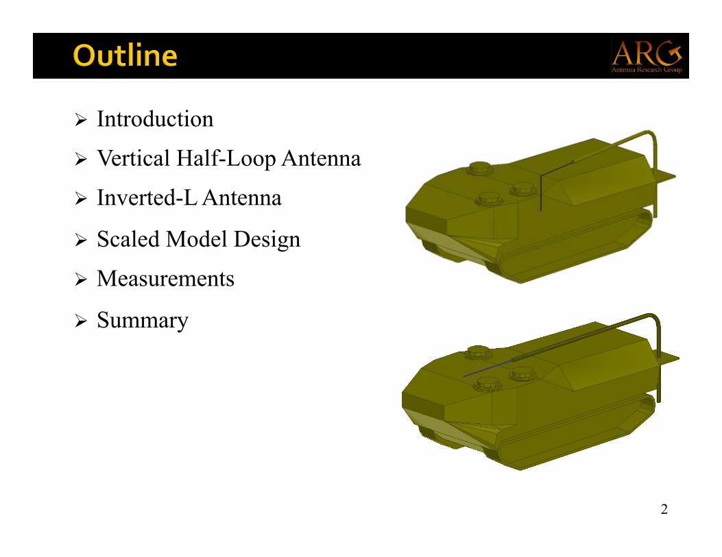
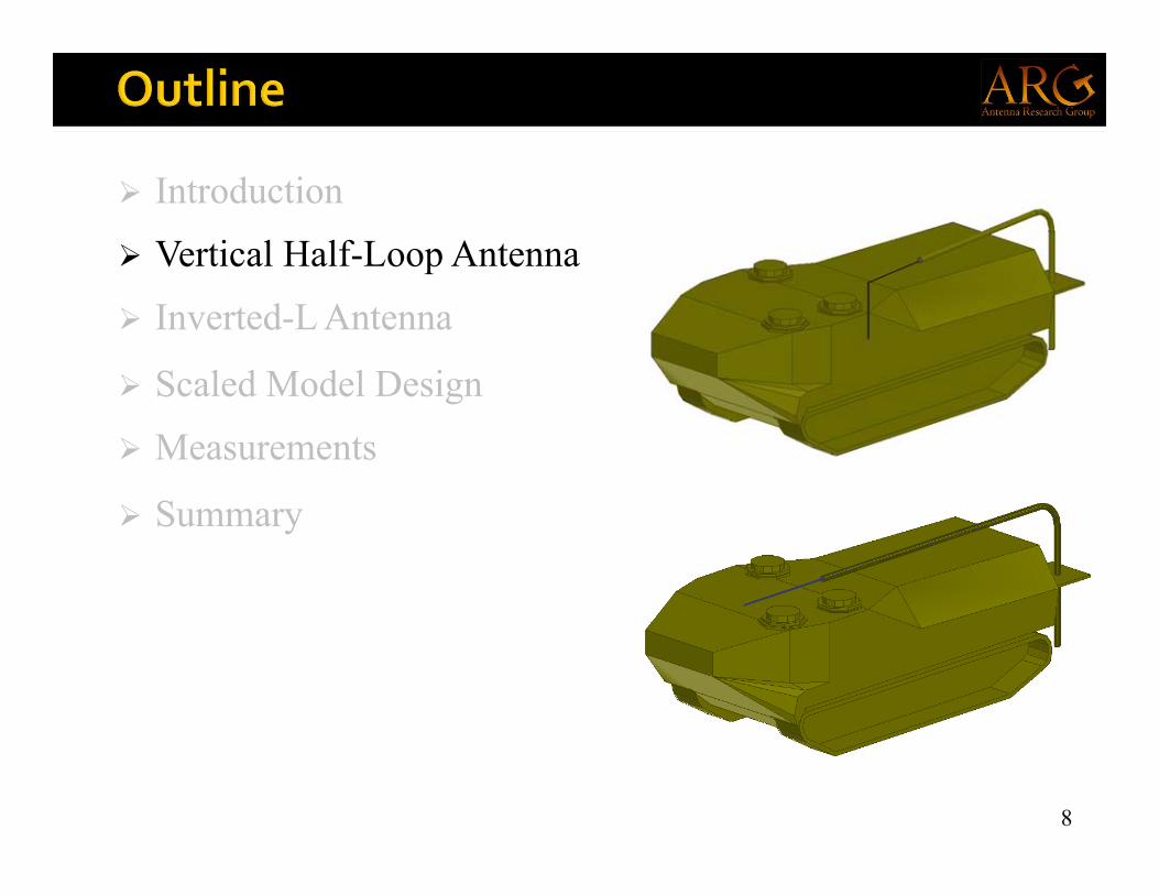
Introduction

Vertical Half-Loop Antenna

Inverted-L Antenna

Scaled Model Design

Measurements

Summary

3

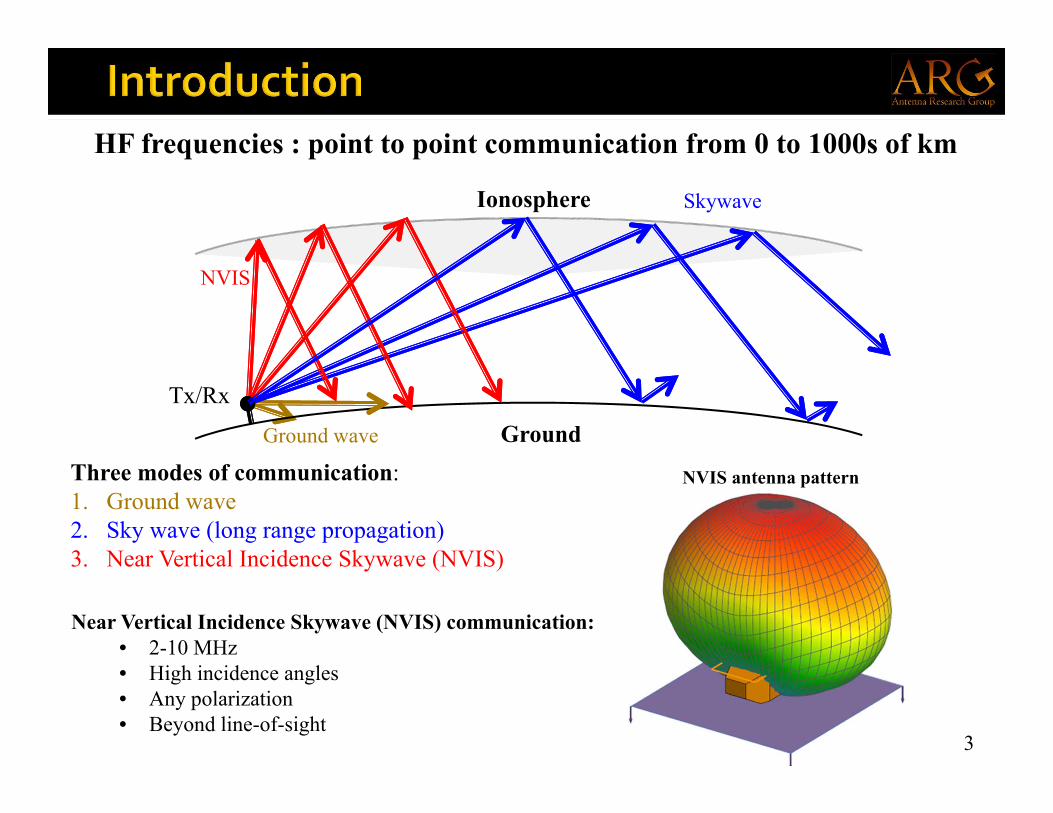
HF frequencies : point to point communication from 0 to 1000s of km

Three modes of communication:1. Ground wave2. Sky wave (long range propagation)3. Near Vertical Incidence Skywave (NVIS)

Ionosphere

GroundTx/Rx

Ground wave

NVIS

Skywave

Near Vertical Incidence Skywave (NVIS) communication:• 2-10 MHz• High incidence angles• Any polarization• Beyond line-of-sight

NVIS antenna pattern

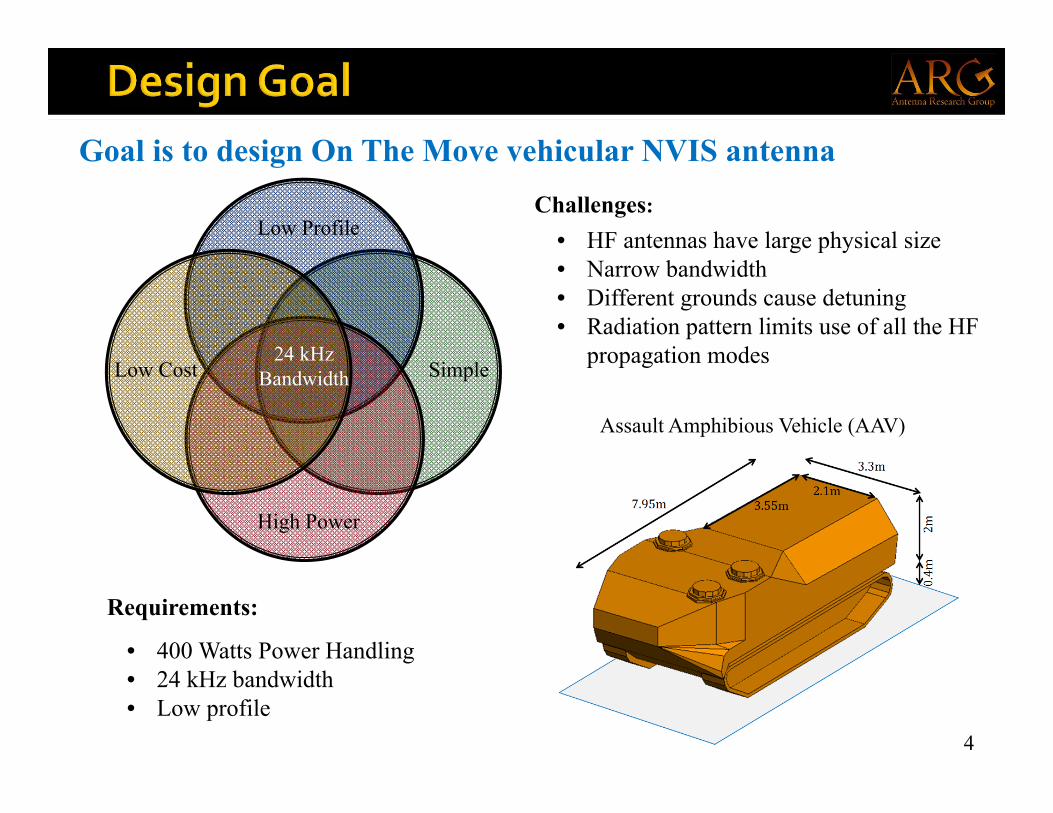
Requirements:

• 400 Watts Power Handling• 24 kHz bandwidth• Low profile

Assault Amphibious Vehicle (AAV)

4

Goal is to design On The Move vehicular NVIS antenna

SimpleLow Cost

Low Profile

24 kHzBandwidth

High Power

Challenges:

• HF antennas have large physical size• Narrow bandwidth• Different grounds cause detuning• Radiation pattern limits use of all the HF

propagation modes

AAV

Spherical antenna

Loop

Dipole

14m

23m

39m

5

[1] M. Gustaffson et al., “Physical Limitations on Antennas of Arbitrary Shape,” Proc. Royal Society A, (2007)

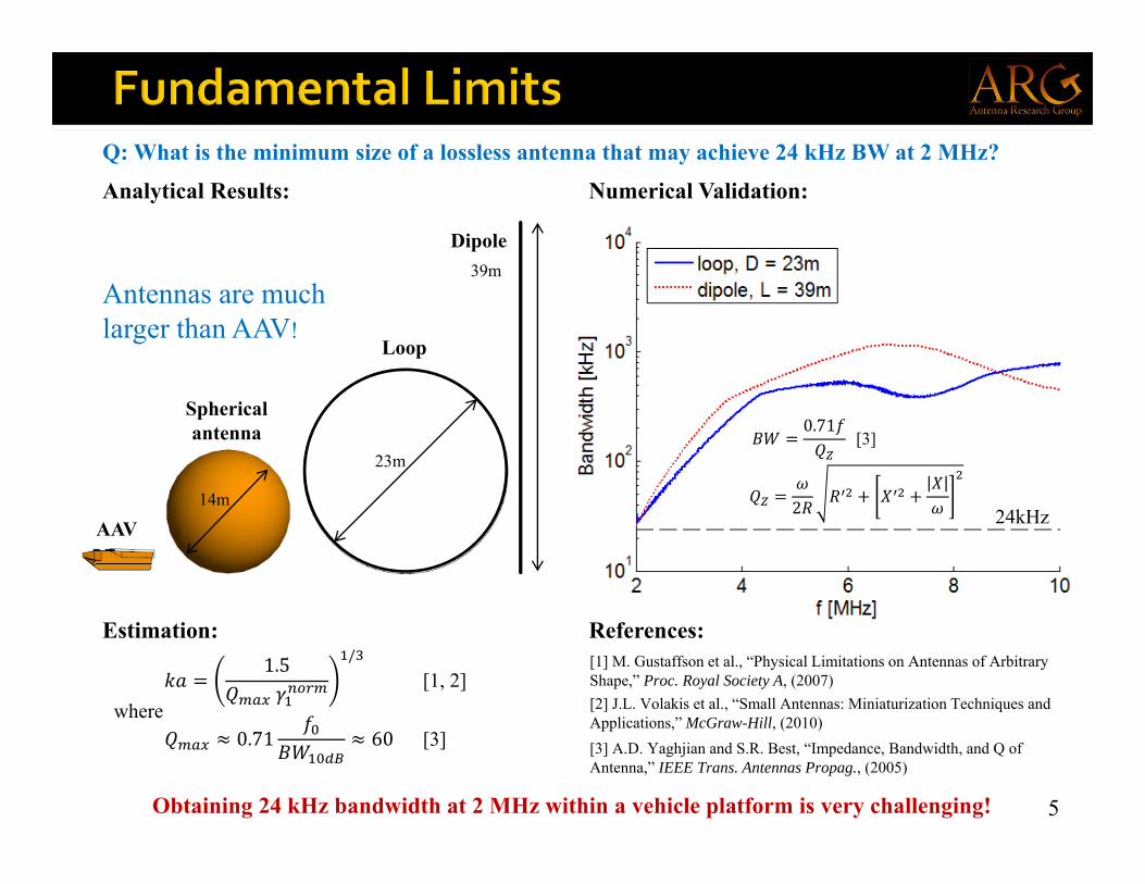
0.71 60

1.5

/

[3] A.D. Yaghjian and S.R. Best, “Impedance, Bandwidth, and Q of Antenna,” IEEE Trans. Antennas Propag., (2005)

[2] J.L. Volakis et al., “Small Antennas: Miniaturization Techniques and Applications,” McGraw-Hill, (2010)

[3]

[1, 2]

Q: What is the minimum size of a lossless antenna that may achieve 24 kHz BW at 2 MHz?

Antennas are much larger than AAV!

Estimation:

Analytical Results:

References:

where

Obtaining 24 kHz bandwidth at 2 MHz within a vehicle platform is very challenging!

24kHz

Numerical Validation:

2

0.71[3]

6

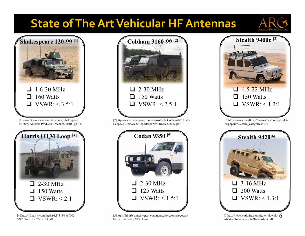
Stealth 9400c [3]

4.5-22 MHz 150 Watts VSWR: < 1.2:1

Codan 9350 [5]

2-30 MHz 125 Watts VSWR: < 1.5:1

2-30 MHz 150 Watts VSWR: < 2.5:1

Shakespeare 120-99 [1] Cobham 3160-99 [2]

Harris OTM Loop [4] Stealth 9420[6]

3-16 MHz 200 Watts VSWR: < 1.3:1

[3]https://www.stealth.ae/plugins/custompages/detinf.php?id=372&id_categories=136

[5]https://hf-ssb-tranceiver.at-communication.com/en/codan/hf_ssb_antennas_9350.html

[6]http://www.cntlwire.com/dealer_downloads/stealth-antennas/9420-datasheet.pdf

[2]http://www.masergroup.com/downloads/Cobham%20Half-Loop%20Demo%20Report%20Nov-Dec%202012.pdf

2-30 MHz 150 Watts VSWR: < 2:1

[4] http://rf.harris.com/media/RF-3134-AT003-5%20Web_tcm26-19129.pdf

1.6-30 MHz 160 Watts VSWR: < 3.5:1

[1]www.Shakespeare-military.com, Shakespeare Military Antenna Products Brochure, 2010. pp-15.

7

[1]

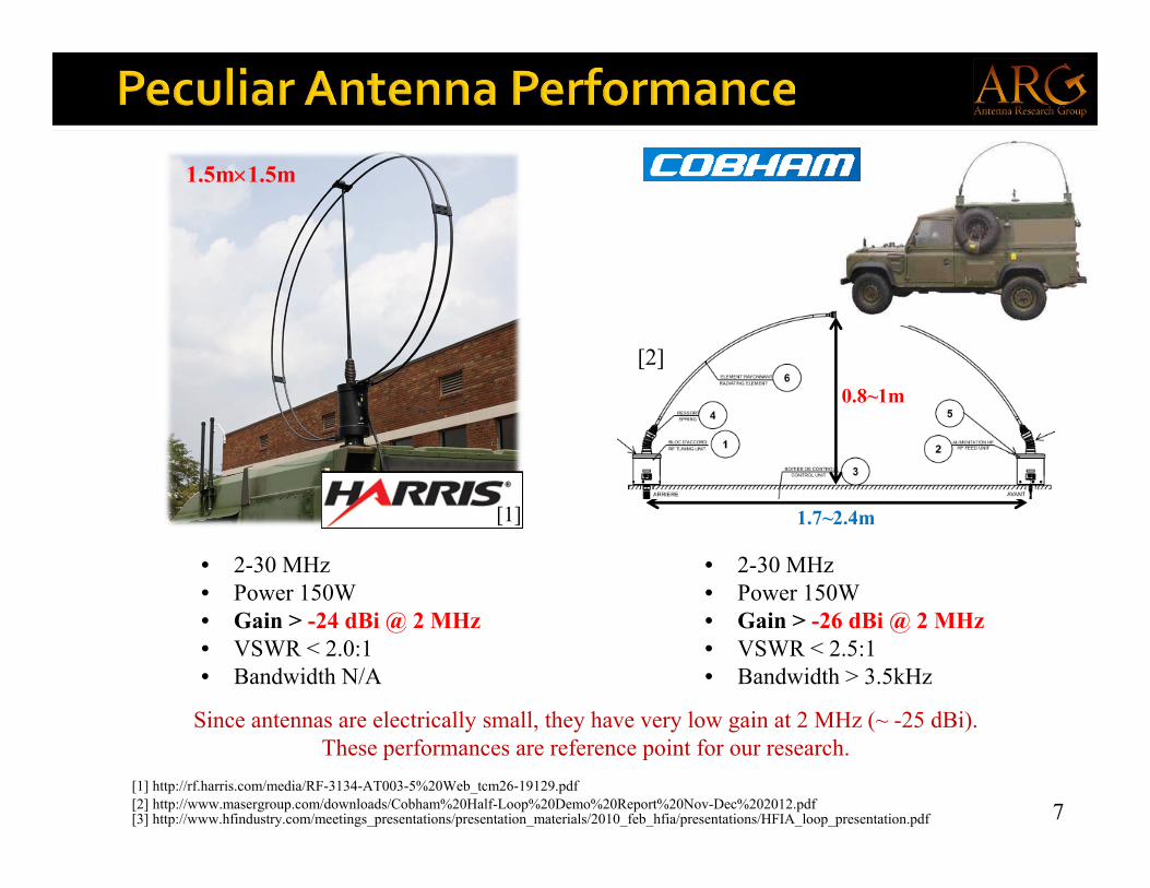
1.5m1.5m

• 2-30 MHz• Power 150W• Gain > -24 dBi @ 2 MHz• VSWR < 2.0:1• Bandwidth N/A

[2] http://www.masergroup.com/downloads/Cobham%20Half-Loop%20Demo%20Report%20Nov-Dec%202012.pdf[1] http://rf.harris.com/media/RF-3134-AT003-5%20Web_tcm26-19129.pdf

[3] http://www.hfindustry.com/meetings_presentations/presentation_materials/2010_feb_hfia/presentations/HFIA_loop_presentation.pdf

Since antennas are electrically small, they have very low gain at 2 MHz (~ -25 dBi).These performances are reference point for our research.

1.7~2.4m

• 2-30 MHz• Power 150W• Gain > -26 dBi @ 2 MHz• VSWR < 2.5:1• Bandwidth > 3.5kHz

[2]0.8~1m

8

Introduction

Vertical Half-Loop Antenna

Inverted-L Antenna

Scaled Model Design

Measurements

Summary

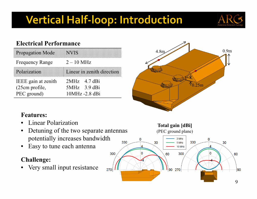
Electrical PerformancePropagation Mode NVIS

Frequency Range 2 – 10 MHz

Polarization Linear in zenith direction

IEEE gain at zenith (25cm profile, PEC ground)

2MHz 4.7 dBi5MHz 3.9 dBi10MHz -2.8 dBi

Features:• Linear Polarization• Detuning of the two separate antennas

potentially increases bandwidth• Easy to tune each antenna

Challenge:• Very small input resistance

Total gain [dBi]

9

(PEC ground plane)

4.8m

0.25m

0.9m

10

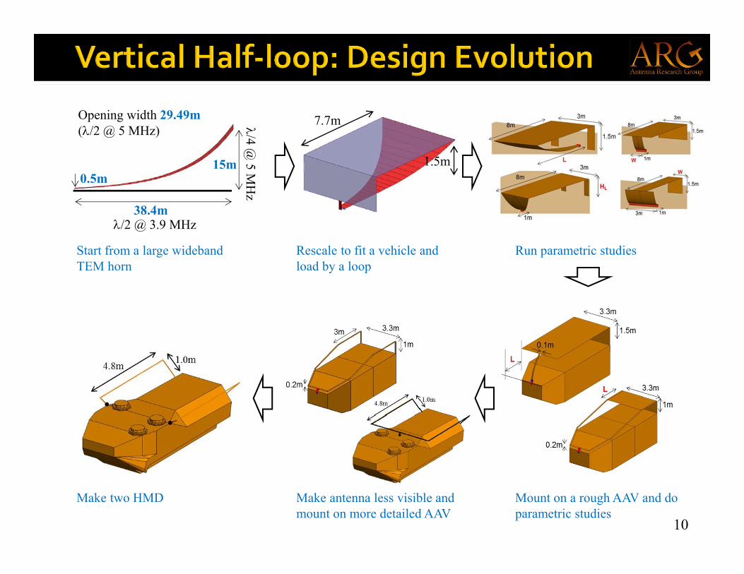
0.5m15m

38.4m

/4 @ 5 M

Hz

/2 @ 3.9 MHz

Opening width 29.49m(/2 @ 5 MHz)

Start from a large wideband TEM horn

Rescale to fit a vehicle and load by a loop

7.7m

1.5m

Run parametric studies

Mount on a rough AAV and do parametric studies

Make antenna less visible and mount on more detailed AAV

Make two HMD

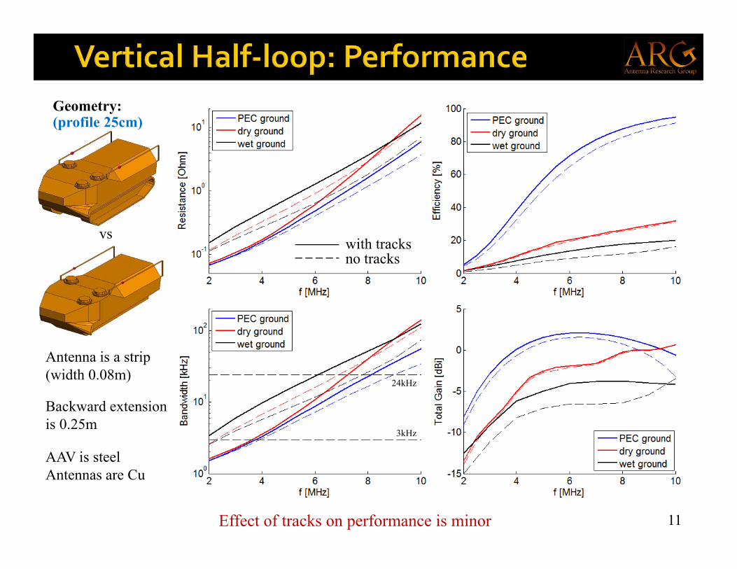
11

24kHz

3kHz

Effect of tracks on performance is minor

Geometry:

Antenna is a strip (width 0.08m)

Backward extension is 0.25m

(profile 25cm)

AAV is steelAntennas are Cu

vswith tracksno tracks

12

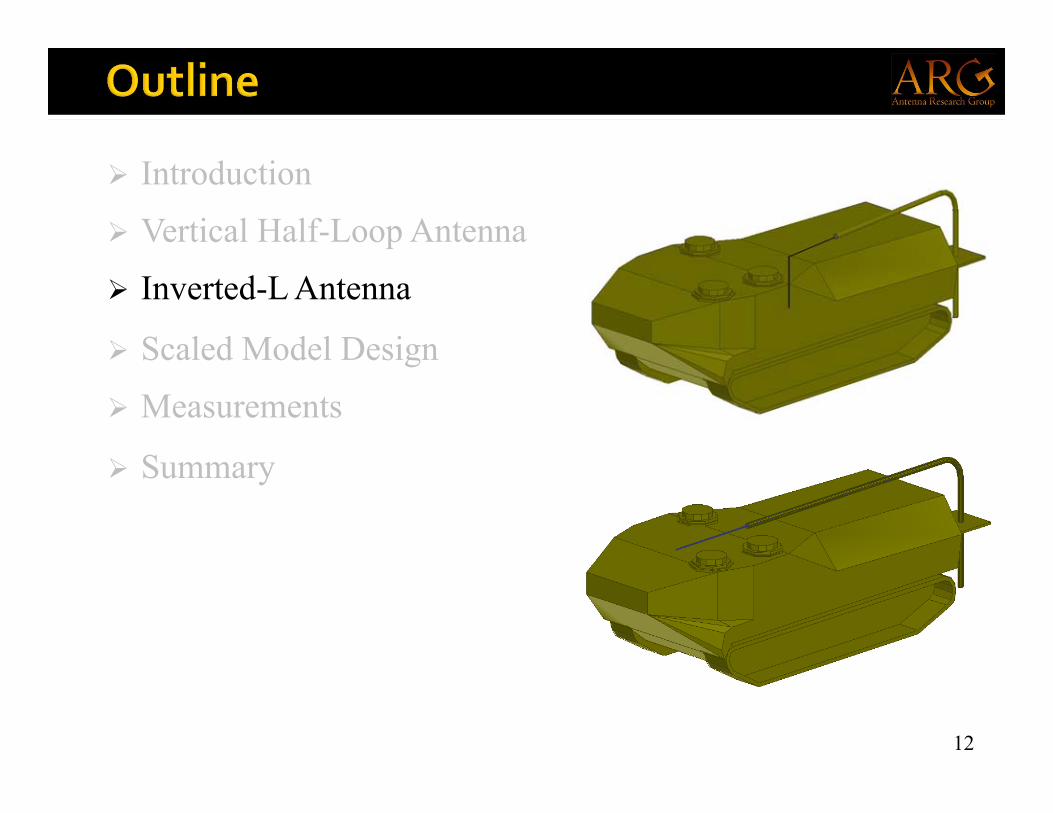
Introduction

Vertical Half-Loop Antenna

Inverted-L Antenna

Scaled Model Design

Measurements

Summary

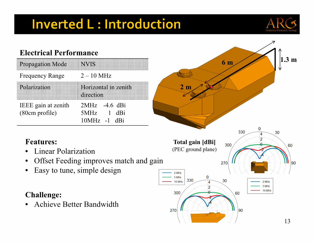
6 m

2 m

1.3 mElectrical PerformancePropagation Mode NVIS

Frequency Range 2 – 10 MHz

Polarization Horizontal in zenith direction

IEEE gain at zenith (80cm profile)

2MHz -4.6 dBi5MHz 1 dBi10MHz -1 dBi

Features:• Linear Polarization• Offset Feeding improves match and gain• Easy to tune, simple design

Challenge:• Achieve Better Bandwidth

Total gain [dBi]

13

(PEC ground plane)

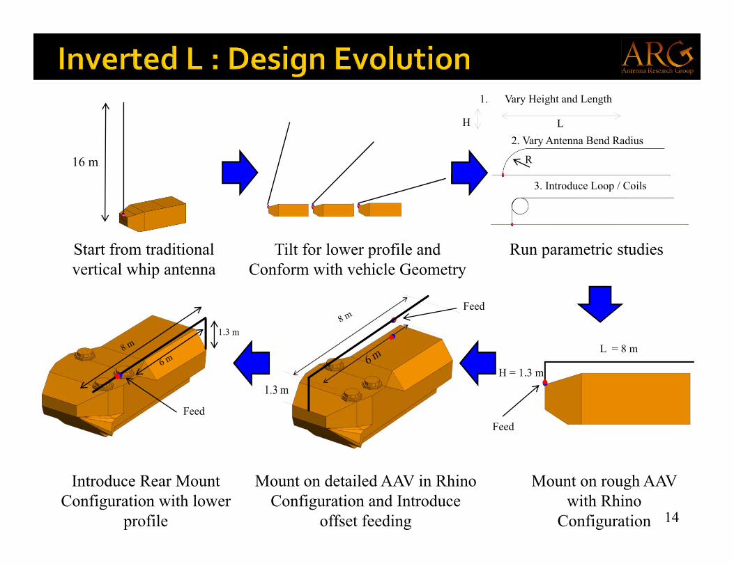
Start from traditional vertical whip antenna

Tilt for lower profile andConform with vehicle Geometry

Run parametric studies

Mount on rough AAV with Rhino

Configuration

Mount on detailed AAV in Rhino Configuration and Introduce

offset feeding

Introduce Rear Mount Configuration with lower

profile

16 m

H = 1.3 m

L = 8 m

Feed

Feed

Feed

1.3 m

2. Vary Antenna Bend RadiusH L

R

3. Introduce Loop / Coils

1. Vary Height and Length

14

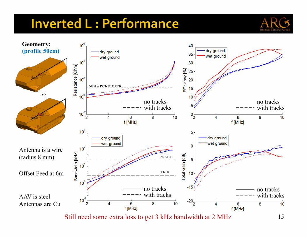
15Still need some extra loss to get 3 kHz bandwidth at 2 MHz

Geometry:

Antenna is a wire (radius 8 mm)

Offset Feed at 6m

(profile 50cm)

AAV is steelAntennas are Cu

vsno trackswith tracks

no trackswith tracks

no trackswith tracks

no trackswith tracks

3 KHz

24 KHz

50 Ω – Perfect Match

16

Introduction

Vertical Half-Loop Antenna

Inverted-L Antenna

Scaled Model Design

Measurements

Summary

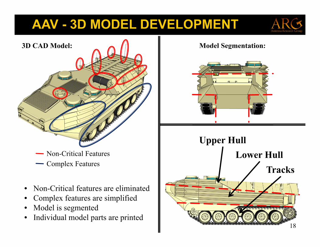
Non-Critical FeaturesComplex Features

3D CAD Model: Model Segmentation:

Upper HullLower Hull

Tracks

• Non-Critical features are eliminated• Complex features are simplified• Model is segmented • Individual model parts are printed

18

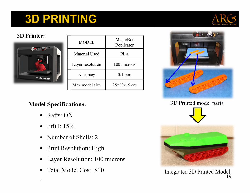
MODEL MakerBotReplicator

Material Used PLA

Layer resolution 100 microns

Accuracy 0.1 mm

Max model size 25x20x15 cm

• Rafts: ON

• Infill: 15%

• Number of Shells: 2

• Print Resolution: High

• Layer Resolution: 100 microns

• Total Model Cost: $10

:

3D Printer:

Model Specifications: 3D Printed model parts

Integrated 3D Printed Model19

19

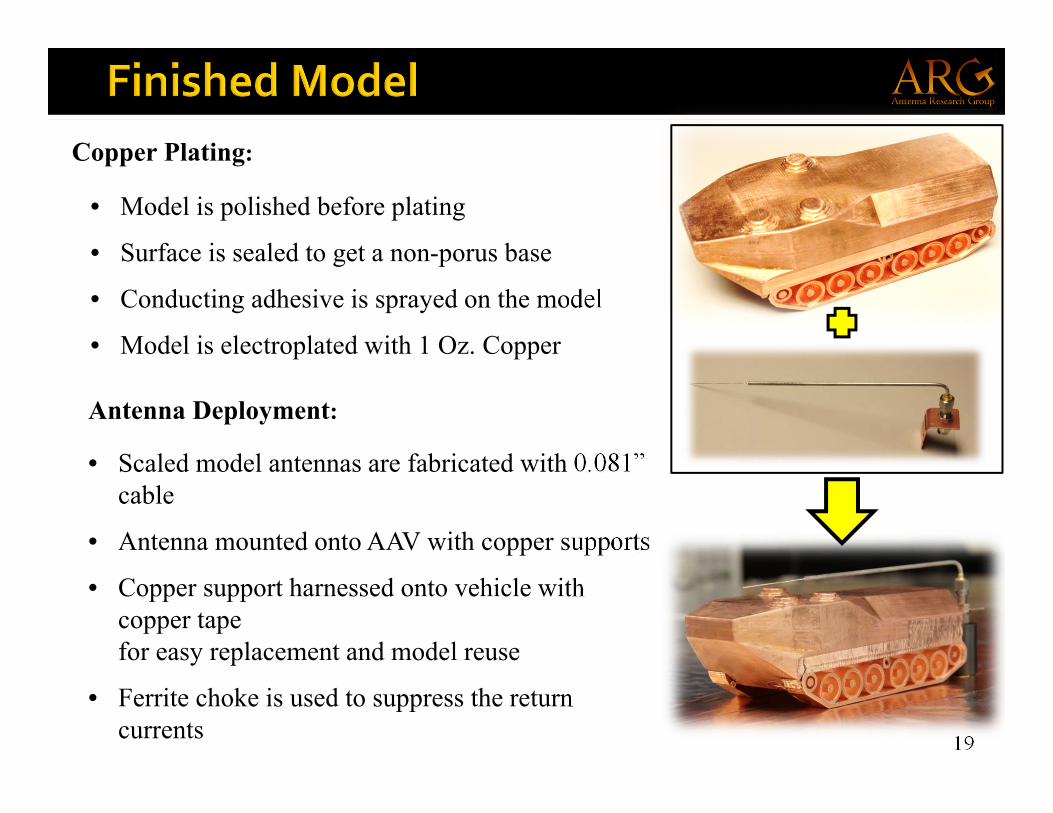
Copper Plating:

• Model is polished before plating

• Surface is sealed to get a non-porus base

• Conducting adhesive is sprayed on the model

• Model is electroplated with 1 Oz. Copper

Antenna Deployment:

• Scaled model antennas are fabricated with 0.081” cable

• Antenna mounted onto AAV with copper supports

• Copper support harnessed onto vehicle with copper tapefor easy replacement and model reuse

• Ferrite choke is used to suppress the return currents

20

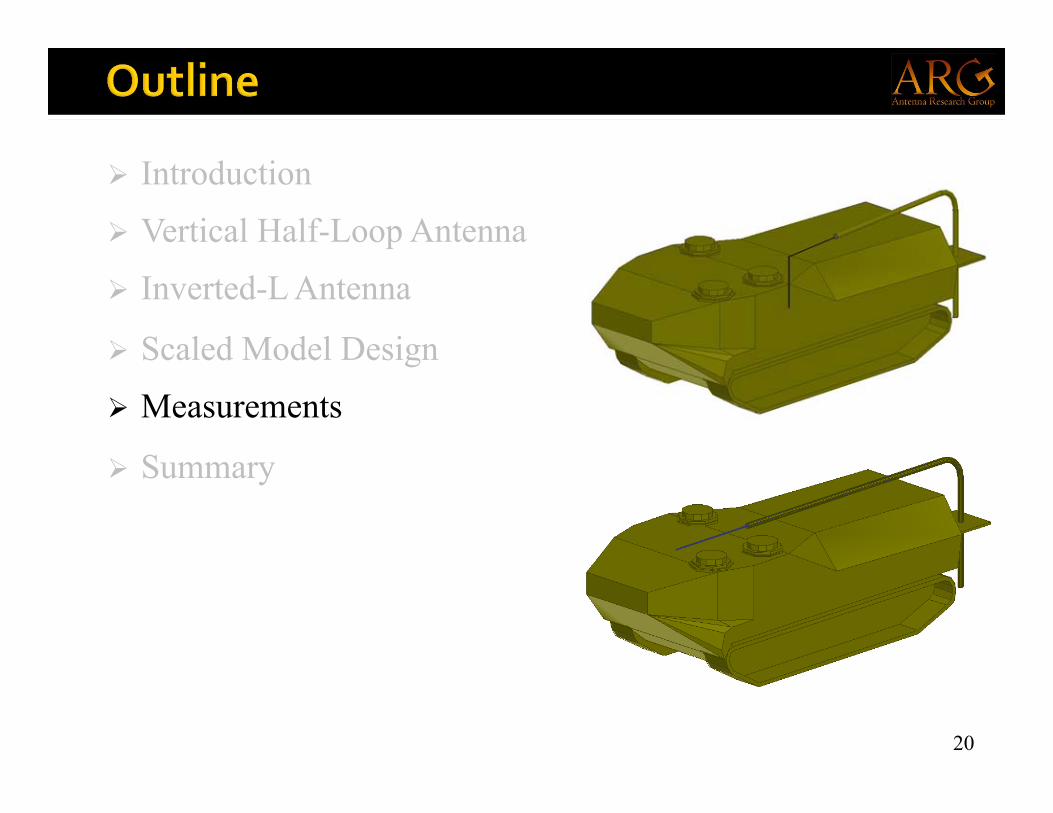
Introduction

Vertical Half-Loop Antenna

Inverted-L Antenna

Scaled Model Design

Measurements

Summary

21

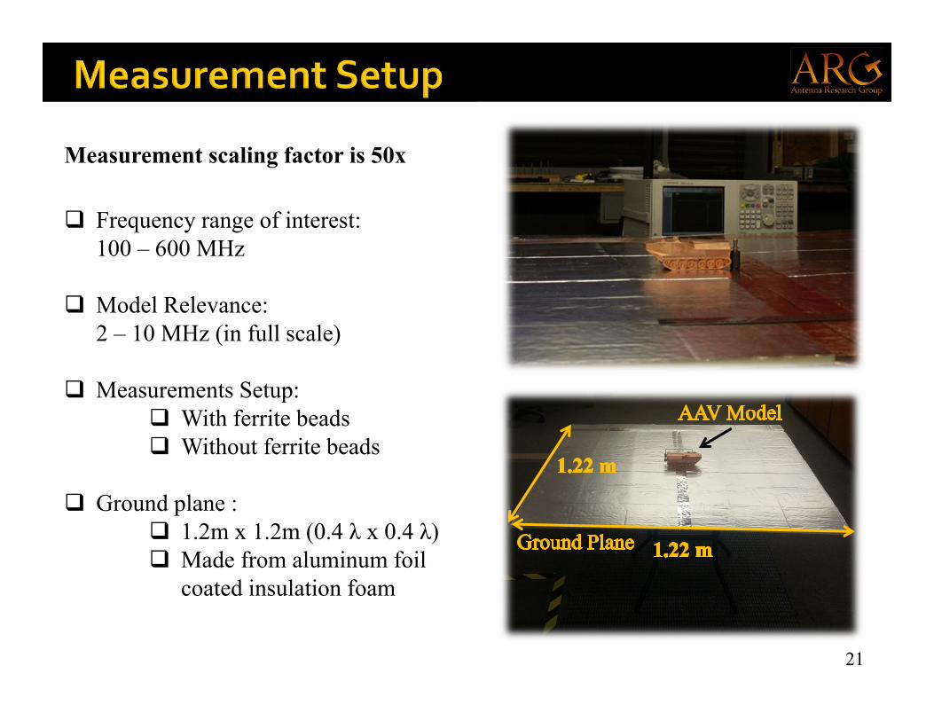
Measurement scaling factor is 50x

Frequency range of interest: 100 – 600 MHz

Model Relevance:2 – 10 MHz (in full scale)

Measurements Setup: With ferrite beads Without ferrite beads

Ground plane : 1.2m x 1.2m (0.4 λ x 0.4 λ) Made from aluminum foil

coated insulation foam

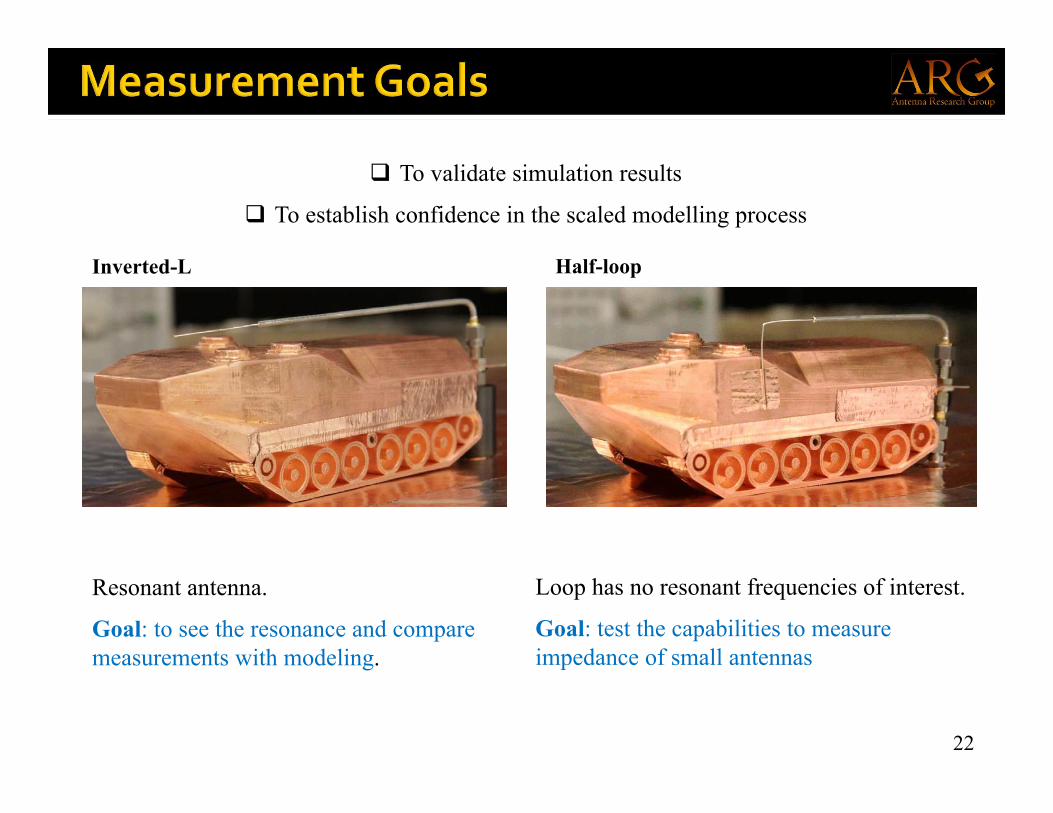
22

Inverted-L

Resonant antenna.

Goal: to see the resonance and compare measurements with modeling.

Half-loop

Loop has no resonant frequencies of interest.

Goal: test the capabilities to measure impedance of small antennas

To validate simulation results

To establish confidence in the scaled modelling process

23

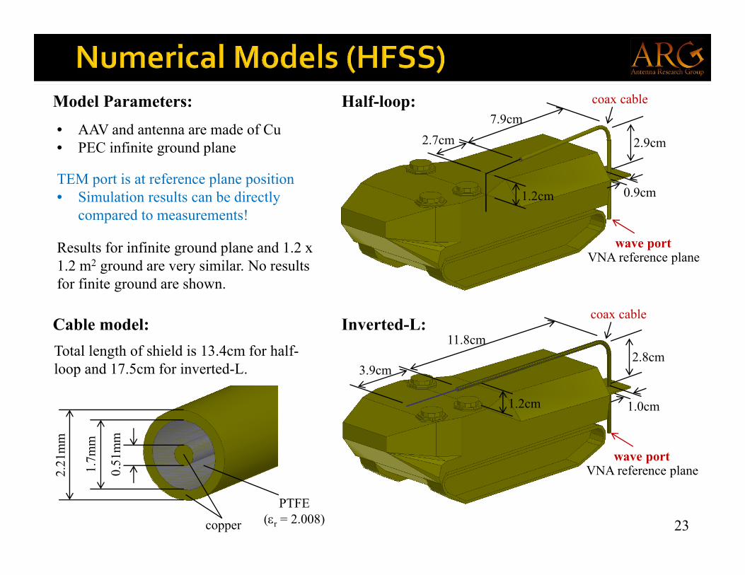
Model Parameters:

2.7cm7.9cm

1.2cm 0.9cm

2.9cm

Half-loop:

Cable model:

wave portVNA reference plane

• AAV and antenna are made of Cu• PEC infinite ground plane

0.51

mm

1.7m

m

2.21

mm

copper

PTFE(r = 2.008)

Total length of shield is 13.4cm for half-loop and 17.5cm for inverted-L.

Inverted-L:

wave portVNA reference plane

2.8cm

1.0cm1.2cm

11.8cm

3.9cm

TEM port is at reference plane position• Simulation results can be directly

compared to measurements!

Results for infinite ground plane and 1.2 x 1.2 m2 ground are very similar. No results for finite ground are shown.

coax cable

coax cable

24

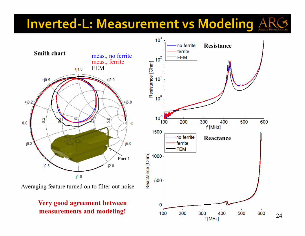
Resistance

Reactance

Smith chart

Very good agreement between measurements and modeling!

FEM

meas., no ferritemeas., ferrite

Port 1

Averaging feature turned on to filter out noise

25

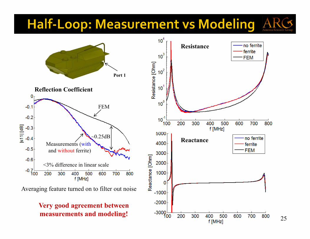
~0.25dB

<3% difference in linear scale

Resistance

Reactance

Reflection Coefficient

FEM

Measurements (withand without ferrite)

Port 1

Averaging feature turned on to filter out noise

Very good agreement between measurements and modeling!

26

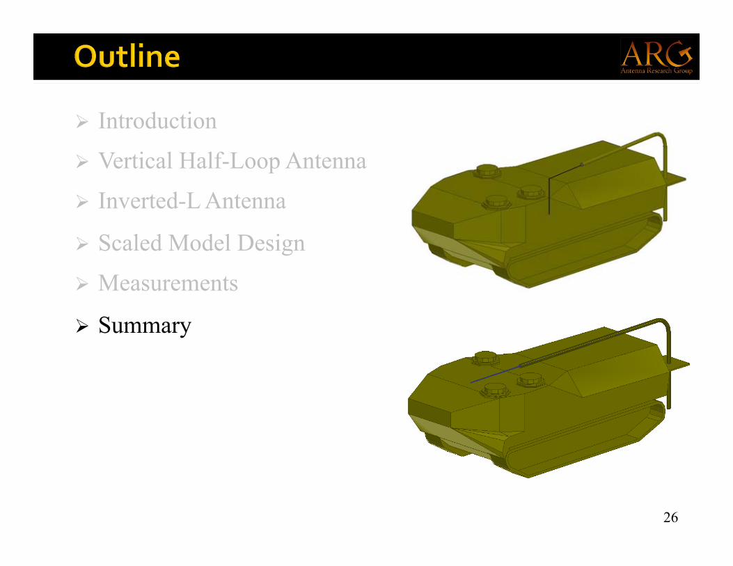
Introduction

Vertical Half-Loop Antenna

Inverted-L Antenna

Scaled Model Design

Measurements

Summary

27

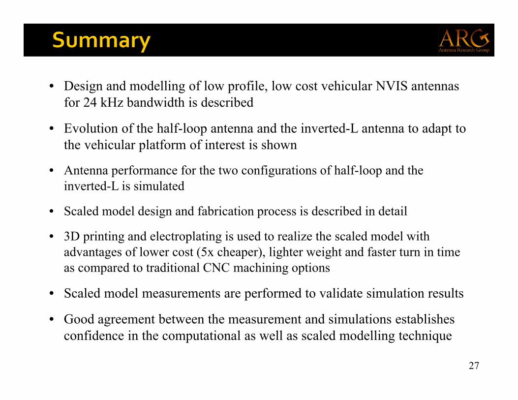
• Design and modelling of low profile, low cost vehicular NVIS antennas for 24 kHz bandwidth is described

• Evolution of the half-loop antenna and the inverted-L antenna to adapt to the vehicular platform of interest is shown

• Antenna performance for the two configurations of half-loop and the inverted-L is simulated

• Scaled model design and fabrication process is described in detail

• 3D printing and electroplating is used to realize the scaled model with advantages of lower cost (5x cheaper), lighter weight and faster turn in time as compared to traditional CNC machining options

• Scaled model measurements are performed to validate simulation results

• Good agreement between the measurement and simulations establishes confidence in the computational as well as scaled modelling technique

QuestionsBooth 18