Saurashtra Universityetheses.saurashtrauniversity.edu/477/1/vaishnani_kp_thesis... · Medical College Rajkot, for the help in conducting biological activities. ... J. C. Javia, N

Saurashtra University Re – Accredited Grade ‘B’ by NAAC (CGPA 2.93)

Vaishanani, Kiritkumar P., 2006, “Physico Chemical Studies of some

Compounds”, thesis PhD, Saurashtra University

http://etheses.saurashtrauniversity.edu/id/eprint/477

Copyright and moral rights for this thesis are retained by the author

A copy can be downloaded for personal non-commercial research or study,

without prior permission or charge.

This thesis cannot be reproduced or quoted extensively from without first

obtaining permission in writing from the Author.

The content must not be changed in any way or sold commercially in any

format or medium without the formal permission of the Author

When referring to this work, full bibliographic details including the author, title,

awarding institution and date of the thesis must be given.

Saurashtra University Theses Service

http://etheses.saurashtrauniversity.edu

[email protected]

© The Author

http://etheses.saurashtrauniversity.edu/id/eprint/477

http://etheses.saurashtrauniversity.edu/

A THESISSUBMITTED TO THE

SAURASHTRA UNIVERSITYFOR THE DEGREE OF

Doctor of PhilosophyIN

THE FACULTY OF SCIENCE ( CHEMSITRY )

BY

KIRITKUMAR P. VAISHNANI

UNDER THE GUIDANCE

OF

Dr. SHIPRA BALUJADr. SHIPRA BALUJADr. SHIPRA BALUJADr. SHIPRA BALUJADr. SHIPRA BALUJA

Department of ChemistrySaurashtra University

Rajkot- 360 005Gujarat - (INDIA)

2006

Doctor of Philosophy

Gram : UNIVERSITY Phone : (R) 2584221 Fax : 0281-2577633 (O) 2578512

SAURASHTRA UNIVERSITYUniversity Road. Rajkot - 360 005.

Dr. Shipra Baluja Residence : M.Sc., Ph.D. 20A/2-Saurashtra University Associate Professor Karmachari Society Department of Chemistry University Road,

Rajkot - 360 005. GUJARAT (INDIA)

No.

Statement under O.Ph.D. 7 of Saurashtra University

The work included in the thesis is my own work under the

supervision of Dr. Shipra Baluja and leads to some contribution in chemistry subsidised

by a nnumber of references.

Dt. : 27 - 02 - 2006 ( KIRITKUMAR P. VAISHNANI )

Place : Rajkot.

This is to certify that the present work submitted for the Ph. D. Degree

University by Kiritkumar P. Vaishnani is his own work and leads to advancement in the

knowledge of chemistry.

The thesis has been prepared under my supervision.

Date : 27 - 02 - 2006 Dr. SHIPRA BALUJA Place : Rajkot. Associate Professor

Department of Chemistry, Saurashtra University Rajkot - 360 005.

ACKNOWLEDGEMENT

Completing of my research work is truly a marathon event and I would not

have been able to complete this journey without the co-operation and support of

countless people over the past three years. I can not find the word to express the

deepest gratitude to my esteemed teacher, adorable guide DR. SHIPRA BALUJA,

Associate Professor, Department of Chemistry, Saurashtra University, Rajkot. Her

invaluable guidance, constructive criticism, motivative attitude, punctuality,

encouragement, tremendous help, parental care and expert supervision throughout

the research work brought my efforts to fruition.

I extend deep sense of gratitude to Prof. H. H. Parekh, Head, Department of

Chemistry, Saurashtra University, Rajkot, for providing necessary facilities and

administrative help.

With a deep sense of gratitude I wish to express my sincere thanks to

Prof. P. H. Parsania, Dr. A. K. Shah, Dr. V. H. Shah, and Shree Hareshbhai

Kundal for their moral support and encouragement.

I would like to extend my thanks to non- teaching staff of Chemistry

Department. Special thanks to Mr. Pankaj Kachhadia for Mass and IR data.

I specially thank Dr. U. V. Manvar, Ex. Dean of Science Faculty,

Saurashtra University, Rajkot, for Stimulating suggestions and encouragement.

I express my sincere thanks to my principal, Shree M. M. Raval, Dean of

Science Faculty, Saurashtra University, Rajkot, Shree J. P. Dholakia, Head,

Department of Chemistry and my all staff members of Bahauddin Science College,

Junagadh, for kind support and providing facilities.

I also consider myself very fortunate to have been provided with invaluable

help and moral support by Shree S. G. Desai, Joint Director, Higher Education,

Gandhinagar.

I wish to express my gratitude to Prof. S. V. Chanda, Department of

Bioscience, Saurashtra University, Rajkot and Dr. Nimish Mungara, P. D. U.

Medical College Rajkot, for the help in conducting biological activities.

I find myself in difficult position to express my deep indebtedness to my

colleagues and friends, Dr. K. M. Rajkotia, Dr. Joshi, Shree G. K. Bera, Dr. D. C.

Karia, Dr. Pranav, Dr. Mayur, Dr. Anjana, Asif, Nikunj, Nirmal, P. K. Kasundra,

J. C. Javia, N. V. Gothi, Dr. Harshad, Sangani, Dr. Vaghela, Nilesh, Janak, Sunil,

Niral, Rahul, Harshad, Bhavin, Dushyant, Bhardavabhai, Chavdabhai, Vazabhai

and Jitendra.

I am thankful to Dr. Narendra V. Patel, Mr. Vipul Chatrabhuji and

Dr. Parimal Chatrabhuji for motivating and giving moral support.

I shall remain indebted to my Parents and Family Members for their

affection and moral support. I get emotional when I think about the sacrifice of my

Wife Rekha and Children during my busy hours.

I express my Sincere thanks to Mr. Rajubhai Solanki for his Excellent Type

Setting and timely completion of these documents.

And finally, still there are many more Well-Wishers, Friends, Relatives, who

directly and indirectly rendered me valuable help and moral strength to complete this

academic endeavour. I have deep reverence for all of them.

Last but not the least, I praise and thank Lord Krishna, Whose benevolent blessing

always keep me on the right track.

Following organization made my task easier due to extension of their facilities :

Director, CDIR - Lucknow. ( Mass and NMR )

R. S. I. C. Nagpur University – Nagpur. ( TGA/ DTA )

R. S. I. C. Punjab University – Chandigarh. ( NMR )

Department of Chemistry, S. P. University,V.V.Nagar. ( DSC )

Department of Chemistry, Saurashtra University, Rajkot. ( Mass and IR )

Department of Bioscience, Saurashtra University, Rajkot. ( Biological

Activities )

P. D. U. Medical College Rajkot. ( Biological Activities )

KIRITKUMAR P. VAISHNANI

CONTENTS

SYNOPSIS PAGE

No.

CHAPTER - I LITERATURE SURVEY ON SYNTHESIS, CHARACTERIZATION AND APPLICATIONS OF SCHIFF BASES AND THIAZOLIDINONES

1-15

CHAPTER - II SYNTHESIS OF SCHIFF BASES AND THIAZOLIDINONES

16-24

CHAPTER - III SPECTRAL CHARACTERIZATION 25- 119

CHAPTER - IV DETERMINATION OF PHYSICOCHEMICAL PROPERTIES

SECTION – 1 HEAT OF SOLUTION 120-125

SECTION - 2 DENSITY 126-140

SECTION - 3 CONDUCTANCE 141-156

SECTION - 4 DISSOCIATION CONSTANTS 157-184

SECTION - 5 ACOUSTICAL PROPERTIES 185-215

SECTION - 6 THERMAL PROPERTIES 216-244

CHAPTER - V BIOLOGICAL ACTIVITIES 245-254

CHAPTER - VI A COMPREHENSIVE SUMMARY OF THE WORK

255-257

LIST OF PAPERS COMMUNICATED 258

0

CHAPTER - I

LITERATURE SURVEY

ON SYNTHESIS, CHARACTERIZATION

AND APPLICATIONS OF SCHIFF

BASES

AND THIAZOLIDINONES

1

Introduction :

The importance and uses of physicochemical properties are well

recognized. The applications and implications of compounds in certain

systems can be decided only if their physico chemical properties are known.

The major differences among behavioral profiles of molecules in the

environment are attributable to their physicochemical properties. For most

chemicals, only fragmentary knowledge exists about those properties that

determine the application of a compound. A chemical-by-chemical

measurement of the required properties is not practical because of expense.

Further, trained technicians and adequate facilities are not available for

measurement efforts involving thousands of chemicals. In fact, physical and

chemical properties have only actually been measured for about 1 percent of

the approximately 70,000 industrial chemicals. Hence, the need for physical

and chemical constants of chemical compounds has greatly accelerated in

industries, which are always in search of economical and better chemicals.

Although considerable progress has been made in process elucidation

and modeling for chemical processes[1-5], such as photolysis and hydrolysis,

only for a limited number of compounds reliable estimates of the related

fundamental thermodynamic and physicochemical properties (i.e.,

rate/equilibrium constants, distribution coefficient, solubility in water, etc.)

have been achieved. The values of these latter parameters, in most

instances, must be derived from measurements or from the expert judgment

of specialists in that particular area of chemistry. Nowadays, computer

programs are also available to estimate a variety of reactivity parameters[6-14].

This capability crosses chemical family boundaries to cover a broad range of

organic compounds.

The majority of the reactions occurring in solutions are of chemical or

biological in nature. It was previously presumed that solvent only provides an

inert medium for chemical reactions. The significance of solute-solvent

interactions was realized only recently as a result of extensive studied in

aqueous, non aqueous and mixed solvents. Ion-solvent and ion-ion

interactions play a major role in determining the behavior of solutes in

2

solutions[15-18]. In recent years, there has been an increasing interest in the

behavior of solutes in non-aqueous and mixed solvents with a view to

investigating ion-ion and ion-solvent interactions under varied conditions[19].

Fundamental research on non-aqueous electrolyte solutions has

catalyzed their wide technical applications in many fields. Non-aqueous

electrolyte solutions are competing with other ion conductors, especially at

ambient and at low temperatures, due to their high flexibility based on the

choice of numerous solvents, additives and electrolytes with widely varying

properties. However, different sequence of solubility, difference in solvating

power and possibilities of chemical or electrochemical reactions unfamiliar in

aqueous chemistry have open vistas for physical chemists and interest in

these organic solvents transcends the traditional boundaries of inorganic,

organic, analytical and physical chemistry.

The proper understanding of the interactions in solutions would form

the basis of explaining quantitatively the influence of the solvent and the

extent of interactions of ions in solvents and thus pave the way for real

understanding of different phenomena associated with solution chemistry.

These interactions in solutions can be interpreted by conductance, density,

viscosity, and acoustical data. The changes in ionic solvation have important

applications in organic and inorganic synthesis, study of reaction

mechanisms, non aqueous battery technology and extraction.

The density, specific volume, molecular mass and refractive index are

useful in the evaluation of various thermodynamic properties of chemical

materials. The values of heat of solution of different solutes in different

solvents are very much useful in industries. Further, solubilities and Henry's

Law constants[20-26] are also important properties for the application of various

compounds.

Knowledge of the acid-base ionization properties of organic molecules

is essential to describing their environmental transport and transformations, or

estimating their potential environmental effects. For ionizable compounds,

solubility, partitioning phenomena and chemical reactivity are all highly

dependent on the state of ionization in any condensed phase. The ionization

3

pKa of an organic compound is a vital piece of information in environmental

exposure assessment. It can be used to define the degree of ionization and

resulting propensity for sorption to soil and sediment that, in turn, can

determine a compound’s mobility, reaction kinetics, bioavailability,

complexation, etc[27].

The measurement of any property of a specimen undergoing a

programmed temperature change is thermal analysis. Thermal analysis

delivers information often unobtainable by other means. It has been used in

many areas of basic and applied research, quality control and acceptance,

prediction and performance evaluation of products. The thermal analysis

kinetic parameters are applied to problems such as failure and service life

prediction, oxidative stability, thermal breakdown, quality assurance and

control, and also optimizing conditions during industrial synthesis and

fabrication[28].

In the present work, the physico chemical properties such as density,

conductance, heat of solution, dissociations constants, thermal kinetics,

acoustical properties etc. of some organic compounds have been studied.

Among the various types of organic compounds, Schiff bases and

Thiazolidinones have been selected for the present study. The selection of

these compounds is due to their applications in various fields.

Day by Day, Schiff bases are known to be applied for human welfare.

Many Schiff bases are known to be useful in perfumery[29], as corrosion

inhibitor[30], as complexing agents(31) and as intermediate in many

reactions[32-35]. Some other applications of Schiff bases have also been

reported in literature in various fields[36-39]. Further, many workers[40-46]

reported a wide range of biological activities of various Schiff bases.

Literature survey shows that various workers synthesized[47-54] Schiff

bases due to their vivid applications. The preparation of some Schiff bases

have been reported by Sawodny et al[55]. Vazquoz et al[56] reported synthesis

of some Schiff bases from glycine and pyridoxal-5’-phosphate, pyridoxal and

5’-deoxy pyridoxal. Tietze synthesized some Schiff bases from 3-acetyl

tetramic acids with ethylene diamine[57]. Synthesis of some tripodal Schiff

4

bases have also been reported[58]. The characterization of synthesized Schiff

bases has been reported to be done by elemental analysis, IR, NMR and

mass spectral data [59-68]. Dash et al studied mass spectra of Schiff bases

derived from p-hydroxy benzaldehyde and their derivatives[69]. Khuhawar et al

studied infrared spectra of some Schiff base polymers derivatives[70]. NMR

study of Schiff bases from 2-hydroxy-1-naphthaldehyde was reported by

Schiff et al[71]. Przybylski et al reported mass spectra of some Schiff bases

from 5-hydroxy-3-oxapentylamine[72].

Various properties of Schiff bases have been reported[73-81]. Mishra and

Gautam[82] reported acoustical properties of some Schiff bases and their

complexes. Siddique et al[83]. also studied ultrasonic properties of some Schiff

bases in CCl4-water, ethanol-water and acetone-water mixtures. Sarkar et al

also studied thermal properties of some Schiff bases [84]. Chantarasiri et al

also reported some physico-chemical properties of hexadentate Schiff base

derived from salicylaldehydes and triethylenetetramine and zinc complexes[85].

Thiazolidinones, which belong to an important group of hetrocyclic

compounds have been extensively explored for their applications. The

thiazolidinones, substituted at 2 and 3 position are reported to exhibit a wide

variety of biological activities such as antibacterial[86,87], antitubercular[88], anti

HIV and anticancer[89], antidiabetic[90], insecticidal[91], herbicidal[92]

anthelmintics[93], cardiovascular[94], antiviral[95], hypnotic[96-98], antifungal[99-101],

antitumor[102], antiulcer[103], local anaesthetic[104] and antimicrobial[105,106].

Due to various biological activities of these compounds, various

workers[107-117] have synthesized thiazolidinones. Several methods for the

preparation of 4-thiazolidinones are nararated in literature [118-124]. Shah and

Trivedi[125] have synthesized thiazolidinones from 4-aryl thiosemicarbazones

by condensing them with chloroacetic acid, a-bromopropionic and a-

bromophenyl acetic acid. Nath and coworkers[126] have prepared 4-

thiazolidinones by cyclization of N-aryl-N’-(2'-pyridyl)-thiocarbamide with

chloroacetic acid. Saeda et al[127]. have synthesized some new

thiazolidinones.

5

Recently, various workers studied their biological properties[128-136].

Lodhi and co-workers[137] have been synthesized and studied antimicrobial,

antiinflammatory and analgesic property of 4-thiazolidinone and arylidene

derivatives. Mogilaiah and co-workers[138] isolated some 4-thiazolidinone

derivatives and tested their antibacterial activity Bhawana et al[139] have

synthesized thiazolidinone derivatives and compared their antiinflammatory

activity, ulcerogenic liability, cardiovascular and CNS effects. Sun et al

elucidated structure-antioxidant activity relationship for some thiazolidinones

derivatives[140]. Kocabalkanli et al also evaluated antimicrobial activities of

some 2, 5-disubstituted -4-thiazolidinones[141]. Kucukguzel et al[142] have

synthesized thiazolidinones as antimicrobial and anticancer agent. Tonghui et

al[143] have documented thiazolidinones as CFTR (cystic fibrosis

transmembrane conductance regulator) inhibitor. Sonawane et al[144] have

also synthesized some new thiaolidinone derivatives as in vivo pharmacology

and studied antidiarrheal efficacy of a thiazolidinone CFTR inhibitor in

rodents. CFTR inhibition of some new thiazolidinones have also been

reported[145,146]. Recently, Dayam et al.(147) have reported some novel

thiazolidinone derivatives as novel class of HIV- integrase inhibitors.

Küçükgüzel et al(148) also reported synthesis and biological activity of some 4-

thiazolidinones.

These valid observations led us to explore the synthesis and physico

chemical properties of some Schiff bases and thiazolidinones.

6

References:

[1] R. G. Zepp and D. M. Cline, Environ. Sci. Technol.,11 (1977) 359.

[2] J. L. Smith, W. R. Mabey, N. Bohanes, B. B. Hold, S.S. Lee, T.W.

Chou, D.C. Bomberger and T. Mill, “ Environmental Pathways of

Selected Chemicals in Fresh Water Systems”, Part11, U.S.

Environmental Protection Agency, Athens, GA (1978).

[3] D. MacKay, A. Bobra, W. Y. Shiu and S. H. Yalkowski, Chemosphere,

9 (1980) 701.

[4] R. G. Zepp. “Handbook of Environmental Chemistry” (Hutzinger,

O.,ed.), Vol.2(B) Springer-Verlag, New York, NY, (1982).

[5] H. Drossman, H. Johnson and T. Mill, Chemoshpere, 17 (1987) 1509.

[6] S. W. Karickhoff, V. K. McDaniel, C. M. Melton, A. N. Vellino, D. E.

Nute, and L. A. Carreira, Environ. Toxicol. Chem., 10 (1991)1405.

[7] S. H. Hilal, L. A. Carreira, C. M. Melton and S. W. Karickhoff, Quant.

Struct. Act. Relat. 12 389 (1993).

[8] S. H. Hilal, L. A. Carreira, C. M. Melton, G. L. Baughman and S. W.

Karickhoff, J. Phys. Org. Chem. 7 (1994)122.

[9] S.H. Hilal, L.A. Carreira and S. W. Karickhoff, “Theoretical and

Computational Chemistry, Quantitative Treatment of Solute/Solvent

Interactions”, Eds. P. Politzer and J. S. Murray, Elsevier Publishers,

(1994).

[10] S. H. Hilal, L. A. Carreira, C. M. Melton and S. W. Karickhoff, J.

Chromatogr., 269 (1994) 662.

[11] S. H. Hilal, J. M. Brewer, L. Lebioda and L.A. Carreira, Biochem.

Biophys. Res. Com., 607 (1995) 211.

[12] S. H. Hilal, L. A. Carreira and S. W. Karickhoff, Quant. Struct. Act.

Relat, 14 (1995)348.

7

[13] S. H. Hilal, L. A. Carreira, S. W. Karickhoff , M. Rizk, Y. El-Shabrawy

and N. A. Zakhari, Talanta , 43 (1996) 607.

[14] S. H. Hilal, L. A. Carreira and S. W. Karickhoff, Talanta, 50 (1999)

827.

[15] S. Nishikawa, N. Nakayama and N. Nakao, J. Chem. Soc. Faraday

Trans., 84 (1988) 665.

[16] C. M. Kinart, W. J. Kinart, A. Kolasinski, A. Cwiklinska and T.

Dzikowski, J. Mol. Liq., 88 (2000) 1.

[17] J. I. Bhat and N. S. V. Prasad, Ind. J. Pure App. Phys., 42 (2004) 96.

[18] S. Baluja and A. Shah Fluid Phase Equilibria, 215 (2004) 1, 55.

[19 ] S. K. Bhullar, K. Bhavneet, M. S. Bakshi, S. Jasbir, S. C. Sharma and

I. M. Joshi, Acustica, 73 (1991) 291.

[20] R. F. Rekker, “The Hydrophobic Fragment Constant”, Elsevier,

Amsterdam, Netherlands (1977).

[21] S. Banerjee, S. H. Yalkowski and S. C. Valvani, Environ. Sci. Toxicol.

14 (1980)1227.

[22] W. J. Lyman, W. E. Reehl and D. H. Rosenblatt, “Handbook of

Chemical Property Estimation Methods: Environmental Behavior of

Organic Chemicals”, McGraw-Elill, NewYork, NY. (1982).

[23] M. M. Miller, S. P. Wasik, G. L Huang, W. Y. Shiu and D. Mackay,

Environ. Sci. Technol., 19 (1985) 522.

[24] M. J. Kamlet, R. M. Dougherty, V. M. Abboud, M. H. Abraham and

R.W. Taft, J. Pharm. Sci. 75 (1986) 338.

[25] W. J. Doucette and A.W. Andres, Environ. Sci. Technol., 21 (1987)

821.

[26] G. Shuurmann, Quant. Struct. Act Relat, 9 (1990) 326.

8

[27] S.H. Hilal, S.W. Karickhoff and L.A. Carreira, “ Prediction of Chemical

reactivity parameters and Physical properties of Organic Compounds

from Molecular Structure using SPARC”, Published by U.S.

Environmental Protection Agency (2003)

[28] K. Krishnan, Proc. Nat. Workshop on Thermal Analysis, (2002).

[29] F, V. Well, Am. Perfumar Essent. Oil Rev., 52 (1948) 218.

[30] M. N. Desai and S. T. Desai, J. Electrochem. Soc., 32 (1983) 397.

[31] K. C. Satpathy, A. K. Panda, R. Mishra, A. P. Chopdar and S. K.

Pradhan, J. Ind. Chem. Soc., 71 (1994) 593.

[32] D. E. Metzier, J. E. Longencker and E. E. Snell, J. Am. Chem. Soc.,

75 (1953) 2786.

[33] E. Bayer, Ber, (1975) 2325.

[34] M. Lehtinen, Acta Pharm. Fenn., 89 (1980) 259.

[35] M. Asadi and A. H. Sarvestani, Can. J. Chem., 79 (2001) 1360.

[36] K. Satyanarayana and R. K. Mishra, Anal. Chem., 46 (1974) 1609.

[37] R. Grunes and W. Sawondy, J. Chromatogr, 122 (1985) 63.

[38] J. G. Hu, R. G. Griffin and J. Herzfeld, J. Am. Chem. Soc., 119 (1997)

9495.

[39] T. Poursaberi, L. Hajiagha-Babaei, M. Yousefi, S. Rouhani, M.

Shamsipu, M. Kargar-Razi, A. Moghimi and M. R. Ganjali,

Electroanalysis, 13 (2001) 1513.

[40] F. P. Dwyer, E. Mayhew, E. M. F. Roe and A. Shalman, Brit. J.

Cancer, 19 (1965) 195.

[41] A. K. Mittal and O. P. Singhal, J. Ind. Chem. Soc., LIX (1982) 373.

[42] R. C. Sharma and V. K. Varshney, J. Inorg. Biochem. 41 (1991) 299.

[43] M. Nath and R. Yadav, Bull. Chem. Soc. Jpn., 70 (1997) 331.

[44] S. N. Pandeya, D. Sriram, G. Nath and E. De Clereq, Pharma. Acta

Helv., 74 (1999) 11.

9

[45] S. V. More, D. V. Dongarkhadekar, R. N. Chavan, W. N. Jadhav, S. R.

Bhusare and R. P. Pawar, J. Ind. Chem. Soc., 79 (2002) 768.

[46] K. Dodey, R. J. Anderson, W. J. Lough, D. A. P. Small, M. D. Shelley

and P. W. Groundwater, Bio-org. Med. Chem., 13 (2005) 4228.

[47] K. J. Mehta, A. C. Chawda, A. R. Parikh, J. Ind. Chem. Soc., 56 (1979) 173.

[48] J. Martin, O’Dannell and R. L. Polt, J. Org. Chem., 47 (1982) 2663.

[49] R. L. Polt and M. Peterson, Tetrahedron Lett., 31 (1990) 4985.

[50] C. I. Simionescu, M. Grigoras, I. Cianga and N. Olaru, Eur. Polym. J.,

34 (1998) 891.

[51] R. C. Goyal, K. Arora, D. D. Agarwal and K. P. Sharma, Asian. J.

Chem., 12 (2000) 919.

[52] Y. V. Popov, T. K. Korchagina, G. V. Chicherina and T. A. Ermakova,

Russ, J. Org. Chem., 38 (2002) 350.

[53] N. Sari, S. Arslan, E. Logoglu and I. Sakiyan, G. U. J. Sci., 16 (2003)

283.

[54] R. Kruszynski, M. Siwy, I. P. Czomperlik and A. Trzesowska, Inorg.

Chim. Acta, 359 (2006) 649.

[55] W. Sawodny, M. Reiderer and E. Urban, Inorg. Chim. Acta, 29 (1978)

63.

[56] M. A. Vazquoz, G. Echevarria, F. Morioz, J. Donoso and F. G. Blanco,

J. Chem. Soc. Perkin Trans2, 16 (1989) 17.

[57] O. Tietze, B. Schiofner, B. Ziemer and A. Z. Fresenius, J. Anal. Chem.

357 (1997) 477.

[58] S. Deoghoria, S. Sain, T. K. Karmakar, S. K. Bera and S. K. Chandra,

J. Ind. Chem. Soc., 79 (2002) 857.

[59] K. Ueno and A. E. Martell, J. Phys. Chem., 59 (1955) 998.

[60] M. R. Udupa and G. Aruvamudan, Current. Sci., 42 (1973) 676.

10

[61] R. A. Day, K. Jayasimhuly, J. V. Evans, G. Bhatt, L. C. Lin and M. J.

Wieser, J. Heterocycl. Chem., 17 (1980) 165.

[62] M. S. M. Rawat, J. L. Novula and S. Mal, J. Ind. Chem. Soc., 58 (1981) 652.

[63] J. Canales, C. Olea, G. Mena, J. Varenzulea, J. Castamagna and Y.

J. Vargas, Bol. Soc. Chil. Quim., 35 (1990) 287.

[64] K. M. Yao, W. Zhou, G. Lu and L. F. Shen., J. Chinese. Chem. Soc.,

58 (2000) 1275.

[65] Z. H. Chen and W. C. Tai, Yauji Huaxue, 22 (2002) 350.

[66] S. R. Salman and F. S. Kamounah, Spectroscopy, 17 747 (2003).

[67] S. Chandra and X. Sangeetika, Spect. Chem. Acta, 60 147 (2004).

[68] R. M. Issa, A. M. Khedr and H. F. Rizk, Spectrochim. Acta Part A: Mol.

Biomole. Spectro., 62 (2005) 621.

[69] B. Dash, P. K. Mahapatra, D. Panda and J. M. Pattnaik, J. Ind. Chem.

Soc., 61 (1984) 1061.

[70] M. Y. Khuhawar, A. H. Channar and S. W. Shah, Eur. Polym. J., 34

(1998) 133.

[71] W. Schiff, B. kamienski and T. Driembowska, J. Mol. Struc., 41

(2002) 602.

[72] P. Przybylski, G. Bejcar and B. B. Schroeder, J. Mol. Struc., 245 (2003) 654.

[73] R. Bembi, W. U. Malik and Sushilla, J. Ind. Chem. Soc., LVI (1979)

776.

[74] S. Choudhury, M. Kakoti, A. K. Deb and S. Goswami, Polyhedron, 11

(1992) 3183.

[75] H. Y. Low and H. Ishida, J. Poly. Sci. Part B: Polym. Phys. Mech., 36

(1998) 1935.

11

[76]

S. D. Naikwade, P. S. Mane and T. K. Chondhekar, Asian J. Chem.,

12 (2000) 247.

[77] L. Y. Hong, L. X. Lan, S. Cheng and J. P. Ming, Youji Huaxue, 22

(2002) 482.

[78] A. Maeda, M. A. Verhoeven, J. Lugtenburg, R. B. Gennis, S. P.

Balashov and T. G. Ebrey, J. Phys. Chem., 108 (2004) 1096.

[79] J. P. Costes, J. F. Lamere, C. Lepetit, P. G. Lacroix and F. D. K.

Nakatani, Inorg. Chem., 44 (2005) 1973.

[80] S. M. Sabry, J. Pharma. Biomed. Ana., 40 (2006) 1057.

[81] I. Sheikhshoaie and W. M.F. Fabian, Dyes and Pigments, 70 (2006)

91.

[82] A. P. Mishra and S. K. Gautam, J. Ind. Chem. Soc., 79 (2002) 725.

[83] M. Siddique, M. Idress, P. B. Agarwal, A. G. Doshi, A. W. Raut and M.

L. Narwade, Ind. J. Chem., 42A (2003) 526.

[84] S. Sarkar, Y. Aydogdu, F. Dagdelen, B. B. Bhaumik and K. Dey, Mat.

Chem. Phys., 88 (2004) 357.

[85] N. Chantarasiri, V. Ruangpornvisuti, N. Muangsin, H. Detsen, T.

Mananunsap, C. Batiya and N. Chaichit, J. Mol. Str., 93 ( 2004) 701.

[86] M. B. Hogale, A. C. Uthale and B. P. Nikam, Ind. J. Chem., 30B

(1991) 717.

[87] K. Desai and A. J. Baxi, J. Ind. Chem. Soc., 69 (1992) 212.

[88] M. D. Joshi, M. K. Jani; B. R. Shah, N. K. Undavia, P. B. Trivedi, J.

Ind. Chem. Soc., 67 925 (1990).

[89] J. J. Bhatt, B. R. Shah, H. P. Shah, P. B. Trivedi, N. C. Desai; Ind.J.

Chem., 33B (1994) 189.

[90] J. Albuquerque, F. Cavalkant, L. Azeuedo, S. Galdino, Anna. Pharm.

Fr., 53 (1995) 209.

[91] P. Schauen, A. Krbarae, M. Tisler and M. Likar, Experimental, 22

(1996) 304.

12

[92] G. Mayer, V. L. F. Misslitz, PCT. Int. Appl. WO 02 48 140 (Cl. C07 D

413/60); Chem. Abstr., 137 (2002) 33290v.

[93] A. J. Compet, R. R. Astik, K. A. Thaker, J. Inst. Chem., 53 (1980) 111.

[94] S. P. Singh, S. K. Anyoung and S. S. Parmar; J. Pharm. Sci., 63

(1974) 960.

[95]

T. Takematsu, K. Yokohama, K. Ideda, Y. Hayashi and E. Taniyamal,

Jpn. Patent 7 (1975) 51, 21 431; Chem. Abstr., 84 (1976) 26880w.

[96] C. M. Chaudhary, S. S. Parmar, S. K. Chaudhary, A. K. Chaturvedi, J.

Pharm. Sci., 65 (1976) 443.

[97] S. P. Singh, B. Ali, T. K. Anyoung, S. S. Parmar and De Boegr,

Benjamin, J. Pharm. Sci., 65 (1976) 391.

[98] A. K. Dimri and S. S. Parmar, J. Heterocycl. Chem., 15 (1978) 335.

[99] S. P. Gupta and P. Dureja, J. Ind. Chem. Soc., 55 (1978) 483.

[100] G. Fennech, P. Monforte, A. Chimirri and S. Grasso; J. Heterocycl.

Chem., 16 (1979) 347.

[101] R. P. Rao, Curr. Sci., 35 (1996) 541.

[102] P. Monforte, S. Grasso, A. Chimiri and G. French, Pharmaco Ed. Sci.,

36 (1981) 109.

[103] K. Takao, T. Tadashi and O. Yoshiaki, Ger. Offen., 3 (1981) 26,53;

Chem. Abstr., 94 (1981) 175110d.

[104] A. K. El-Shafi and K. M. Hassan, Curr. Sci., 52, (1983) 633.

[105] E. Picscopo, M. V. Diruno, R. Gagliardi, O. Mazzoni, C. Parrill and G.

Veneruso; Bull. Soc. Ital. Biol. Sper., 65 (1989) 131.

[106] K. Ladva, U. Dave and H. H. Parekh; J. Ind. Chem. Soc., 68 (1991)

370.

[107] A. R. Surry, J. Am. Chem. Soc., 74 (1952) 3450.

[108] J. Rogere and M. Audibert, Bull. Soc. Chim. Fr., (1971) 4021.

13

[109] T. Takematsu, K. Yokohama, K. Ikeda, Y. hayashi and E. Taniyamal,

Jpn. Patent, 7 (1975) 21431;Chem. Abstr., 84 (1976) 26880w.

[110] E. Picscopo, M. V. Diruno, R. Gagliardi, O. Mazzoni, C. Parill and G.

Veneruso, Bull. Soc. Ital. Biol. Sper., 65 (1989) 13; Chem. Abstr., 111

(1989) 170938g.

[111] R. P. Pawar, N. M. Andukar and Y. B. Vibhute, J. Ind. Chem. Soc., 76

171 (1999).

[112] M. G. Vigorita, R. Ottanà, F. Monforte, R. Maccari, A. Trovato, M. T.

Monforte and M. F. Taviano Bioorg. Med. Chem. Let., 11, (2001)

2791

[113] G. Kucukguzel, E. E. Oruc, S. Rollas, F. ahin and A. Ozbek, Eur. J.

Med. Chem., 37 (2002) 197.

[114] F. Norio and A. Fujio; PCT Int. Appl. WO 03 (2003) 57,693; Chem.

Abstr., 139 (2003) 117415u.

[115] Y. U. Rassukaua, P. P. Onysko, K. O. Davydova and A. D. Sinitsa,

Eur. J. Org. Chem., 2004 (2004) 3643.

[116] R. Ottana, R. Maccari, M. L. Barreca, G. Bruno, A. Rotondo, A. Rossi,

G. Chiricosta, R. D. Paola, L. Sautebin, S. Cuzzocrea and M. G.

Vigorita, Bioorg. Med. Chem., . 13 (2005) 4243.

[117] C.V. Kavitha, Basappa, S. N. Swamy, K. Mantelingu, S. Doreswamy,

M.A. Sridhar, J. S. Prasad and K. S. Rangappa, Bioorg. Med. Chem.,

14 (2006) 2290.

[118] C. Liberman and A. Lange, Ann., 207 (1881) 121.

[119] W. Davies, J. Chem. Soc., (1949) 2633.

[120] H. Erlenmeyers, Helv. Chem. Acta., 39 (1956) 1156.

[121] A. Mystafa, W. Asker, A. F. A. Shalaby and M. E. E. Shobby, J. Org.

Chem., 23 (1958) 1992.

[123] A. R. A. Raouf, M. T. Omar and M. M. ed-Attal, Acta. Chim. Acad. Sci.

Hung, 87 (1975) 187.

14

[124 ]

E. Fisher, I. Hartmann and H. Priebs, Z. Chem., 15 480 (1975); Chem.

Abstr., 84 1 (1976) 5553f.

[125] I. D. Shah and J. P. Trivedi, J. Ind. Chem. Soc., 40 (1963) 889.

[126] R. Nath, K. Shanker, R. C. Gupta and K. Kishor; J. Ind. Chem. Soc.,

55 (1978) 832.

[127]

M. Saeda, M. Abdel-Megid and I. M. El-Deen, Ind.J. Heterocyc.

Chem., 2 (1993) 81.

[128] K. Mogilaiah and R. Babu Rao, Ind. J. Chem., 37B (1998) 894.

[129] H. V. Hassan, N. A. El-Koussi, Z. S. Farghaly; Chem. Pharm. Bull., 46

(1998) 863.

[130] G. G. Bhatt and C. D. Daulatabad; Ind. J. Heterocycl. Chem., 9 (1999)

157.

[131] V. S. Ingle, R. D. Ingle and R. A. Mave; Ind. J. Chem., 40B 124

(2001).

[132] M. Siddique, M. Indress, A. G. Doshi; Asian J. Chem., 14 (2002) 181.

[133] X. F. Wang, M. M. Reddy and P. M. Quinton, Exp Physiol. 89 (2004)

417.

[134] M. H. Shih and F. Y. Ke, Bioorg. Med. Chem. 12 (2004) 4633.

[135] D. Reigada and C. H. Mitchell, Am. J. Physiol Cell Physiol. 288 (2005)

2005.

[136] P. Vicini, A. Geronikaki, K. Anastasia, M. Incerti and F. Bioorg.and

Med. Chem., In Press, (2006)

[137]

R. S. Lodhi, S. D. Srivasatava and S. K. Srivastava; Ind. J. Chem.,

37B (1998) 899.

[138]

K. Mogilaiah, R. Babu Rao and K. N. Reddy; Ind.J. Chem., 38B

(1999) 818.

[139] G. Bhawana, R Tilak, T Ritu, A. Kumar, E. Bansal, Eur. J. Med.

Chem., 34 (1999) 256.

15

[140] Y. M. Sun, X. L. Wang, H. Y. Zhang and D. Z. Chen, Quant. Struc.

Activity Relation., 20 (2001) 139.

[141] A. Kocabalkanli, O. Ates and G. Otuk, Archiv der Pharmazie, 334

(2001) 35.

[142] S. G. Kucukguzel, E. E. Oruc, S. Rollas, F. Sahin and A. Ozbek, Eur.

J. Med. Chem., 37 (2002) 197.

[143] T. Ma, J. R. Thiagarajah, H. Yang and N. D. Sonawane, J. Clinical

Invest., 110 (2002) 1651.

[144] N. D. Sonawane, C. Muanprasat, Jr. R. Nagatani, Y. Song and A. S.

Verkman, J. Pharm. Sci. 94 (2004) 134.

[145] A. Taddei, C. Folli, O. Zegarra-Moran, P. Fanen, A. S. Verkman and

L. J. Galietta, FEBS Lett. 558 (2004) 52.

[146] D. B. Salinas, N. Pedemonte, C. Muanprasat, W. F. Finkbeiner and D.

W. Nielson, Am. J. Physiol Lung Cell Mol Physiol. 287L (2004) 936.

[147] R. Dayam, T. Sanchez, O. Clement, R. Shoemaker, S. Sei and N.

Neamati, J. Med. Chem. 48 (2005) 111.

[148] G. Kucukguzel, A. Kocatepe, E. D. Clercq, F. Sahin and M. Gulluce

Eur. J. Med. Chem., In Press (2006)

CHAPTER - II

SYNTHESIS OF

SCHIFF BASES AND THIAZOLIDINONES

16

The following Schiff bases have been synthesized from p-amino

phenol.

1 KPV-1 2-[(4-hydroxyphenyl)imino]methyl phenol

2 KPV-2 4-[(2-chlorophenyl)methylene]aminophenol

3 KPV-3 4-[(4-methoxyphenyl)methylene]aminophenol

4 KPV-4 4-[(2-nitrophenyl)methylene]amino phenol

5 KPV-5 4-[(3-nitrophenyl)methylene]aminophenol

6 KPV-6 4-[2-furylmethylene]aminophenol

7 KPV-7 4-[(4-chlorophenyl)methylene]aminophenol

8 KPV-8 4-[(4-hydroxyphenyl)imino]methyl-2-methoxyphenol

17

Synthesis of Schiff bases from p-amino phenol :

The requisite amount of aldehyde, dissolved in 20 ml methanol was

added to 0.1 mole of p-aminophenol and few drops of glacial acetic acid,

which acts as a catalyst. The mixture was refluxed for 10-12 hours at 70-80oC

in water bath.

The resulting solution was cooled to room temperature, and then

poured in crushed ice with constant stirring. The precipitate was filtered and

washed with Sodium bisulfite solution to remove excess of aldehyde. The

product was crystallized from hot methanol and dried.

R-CHO +

N

OH

CH RNH2

OH

where R =

OH Cl

KPV - 1

KPV - 4

OCH3

KPV - 7

NO2

KPV - 3

NO2

OH

OCH3

KPV - 5

KPV - 8

Cl

O

KPV - 2

KPV - 6

18

The physical constants of the synthesized Schiff bases are reported in Table

2.1.

Table 2.1 : Physical constants of KPV Schiff bases.

Compound Code

Molecular Formula

Molecular

Weight g

M.P. OC

% Yield

Rf* Value

KPV-1 C13 H11 N O2 213.235 140 58.7 0.64*

KPV-2 C13 H10 Cl N O 231.678 122 62.5 0.58*

KPV-3 C14 H13 N O2 227.259 165 67.8 0.44+

KPV-4 C13 H10 N2 O3 242.230 166 60.5 0.61*

KPV-5 C13 H10 N2 O3 242.230 162 66.7 0.65*

KPV-6 C11 H9 N O2 187.195 214 54.3 0.62#

KPV-7 C13 H10 Cl N O 231.678 210 53.6 0.44+

KPV-8 C14 H13 N O3 243.258 182 61.4 0.64+

* Ethyl acetate : Benzene - 2.0 : 8.0

+ Acetone : Benzene - 1.0 : 9.0

# Acetone : Benzene - 0.3 : 9.7

19

The following Schiff bases have been synthesized from p-fluoro

aniline.

1 RKV- 1 2-[(4-fluorophenyl)imino]methylphenol

2 RKV- 2 4-[(4-fluorophenyl)imino]methylphenol

3 RKV- 3 4-fluoro-n-[-(2-nitrophenyl)methylene]aniline

4 RKV- 4 N-[-(2-chlorophenyl)methylene]-4-fluoroaniline

5 RKV- 5 N-[-(4-chlorophenyl)methylene]-4-fluoroaniline

6 RKV- 6 4-[(4-fluorophenyl)imino]methyl-n,n-dimethyl-aniline

7 RKV- 7 4-fluoro-n-[-(4-methoxyphenyl)methylene]aniline

8 RKV- 8 4-[(4-fluorophenyl)imino]methyl-2-methoxyphenol

20

Synthesis of Schiff bases from p-fluoro aniline :

The requisite amount of aldehyde, dissolved in 20 ml methanol was

added to 0.1 mole of p-fluoro aniline and few drops of glacial acetic acid,

which acts as a catalyst. The mixture was refluxed for 10-12 hours at 70-80oC

in water bath.



washed with Sodium bisulfite solution to remove excess of aldehyde. The

product was crystallized from hot methanol and dried.

R-CHO +

N

F

CH RNH2

F

Where R =

OH

Cl

RKV - 1

OCH3

NO2

RKV - 3

OH

OCH3

RKV - 5

RKV - 8

Cl

OH

NH3C CH3

RKV - 2

RKV - 6RKV - 4

RKV - 7

21

The physical constants of the synthesized Schiff bases are reported in Table

2.2.

Table 2.2 : Physical constants of RKV Schiff bases.

Compound Code

Molecular Formula

Molecular

Weight g

M.P. OC

% Yield

Rf* Value

RKV-1 C13 H10F N O 215.22 64 71.2 0.52 *

RKV-2 C13 H10F N O 215.22 164 58.5 0.61 *

RKV-3 C13 H9 N2 O2 244.22 63 65.8 0.59#

RKV-4 C13 H9ClFN 233.67 54 42.3 0.63*

RKV-5 C13 H9ClFN 233.67 60 57.5 0.49*

RKV-6 C15H15FN2 242.29 71 65.2 0.58#

RKV-7 C14H12FN O 229.25 52 59.6 0.62#

RKV-8 C14 H12FN O2 245.25 93 62.0 0.51#

* Acetone : Benzene - 1.0 : 9.0

# Acetone : Benzene - 1.5 : 8.5

22

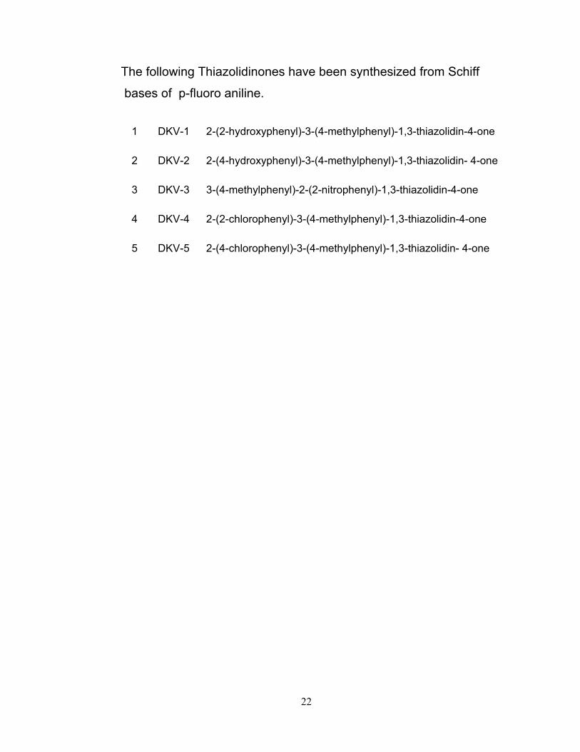
The following Thiazolidinones have been synthesized from Schiff

bases of p-fluoro aniline.

1 DKV-1 2-(2-hydroxyphenyl)-3-(4-methylphenyl)-1,3-thiazolidin-4-one

2 DKV-2 2-(4-hydroxyphenyl)-3-(4-methylphenyl)-1,3-thiazolidin- 4-one

3 DKV-3 3-(4-methylphenyl)-2-(2-nitrophenyl)-1,3-thiazolidin-4-one

4 DKV-4 2-(2-chlorophenyl)-3-(4-methylphenyl)-1,3-thiazolidin-4-one

5 DKV-5 2-(4-chlorophenyl)-3-(4-methylphenyl)-1,3-thiazolidin- 4-one

23

Synthesis of Thiazolidinones :

The requisite amount of Schiff base dissolved in 20 ml methanol, was

added to 0.1 mole of thio glycolic acid and few drops of glacial acetic acid.

The mixture was refluxed for 10-12 hours at 70-80oC in water bath.



washed with water. The product was crystallized from hot methanol and dried.

R-CH=N-R' + HSCH2COOHN

S

O R

R'

where R’ =

F

and R =

OH

DKV - 2

OH

DKV - 1

NO2

Cl

Cl

DKV - 3

DKV - 4 DKV - 5

24

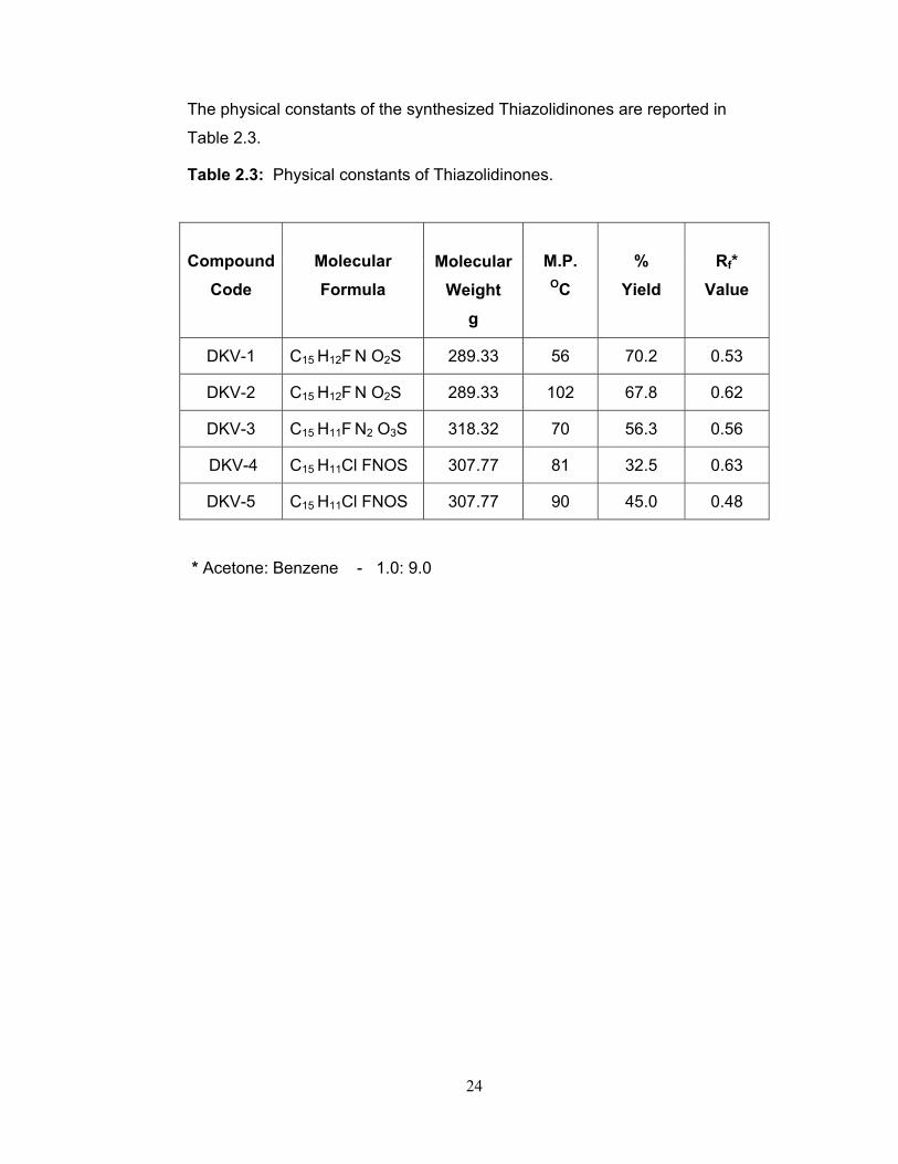
The physical constants of the synthesized Thiazolidinones are reported in

Table 2.3.

Table 2.3: Physical constants of Thiazolidinones.

Compound Code

Molecular Formula

Molecular

Weight g

M.P. OC

% Yield

Rf* Value

DKV-1 C15 H12F N O2S 289.33 56 70.2 0.53

DKV-2 C15 H12F N O2S 289.33 102 67.8 0.62

DKV-3 C15 H11F N2 O3S 318.32 70 56.3 0.56

DKV-4 C15 H11Cl FNOS 307.77 81 32.5 0.63

DKV-5 C15 H11Cl FNOS 307.77 90 45.0 0.48

* Acetone: Benzene - 1.0: 9.0

25

Spectral studies of Schiff bases and Thiazolidinones :

The compounds are well characterized on the basis of infrared (IR), nuclear

magnetic resonance (NMR) and mass spectral data.

Infra-Red Spectra :

Infra-Red spectroscopy is one of the powerful analytical techniques which

offer the possibility of chemical identification.

IR spectrum arises due to excitation of vibrational and rotational energy

levels of the molecular or individual functional groups. It is also called as

“Vibrational Spectroscopy”. IR spectroscopy is an excellent method for the

qualitative analysis because except optical isomers, the spectrum of compound

is unique. It is most useful for the identification of purity and gross structural

details. This method is also useful in the field of natural products, forensic

chemistry and in industrial analysis of competitive products, determination of

force constant, bond strength, identification of compounds, presence of certain

groups in the molecules, identification of hydrogen bonding, study of co-ordination

compounds, polymers and detection of impurity etc.

25 The IR spectra (KBr pellets) of Schiff bases scanned on SHIMADZU

– FT -IR-8400 over the frequency range from 4000-400 cm-1 are shown in Figure

3.1 to 3.21. The characteristic absorption frequencies in cm-1 are given along with

the spectra.

26

0.0

20.0

40.0

60.0

80.0

100.0

%T

500.0750.01000.01250.01500.01750.02000.03250.01/cmsb salicyaldehyde

455.2

497.6 543.9

617.2 698.2

721.3

748.3

829.3

906.5 941.2

968.2

1045.31122.5

1172.61234.4

1276.8

1377.11442.7

1508.2

1593.1

1612.4

2923.93008.7

3066.63097.5

FIG. 3.1 : IR SPECTRAL STUDY OF 2-[(4- HYDROXYPHENYL)IMINO] METHYL PHENOL (KPV-1)

NOH

OH

Type

Vibration mode

Frequency in cm-1

Expected frequency in cm-1 (1-3)

-OH

-O-H (sym.) O-H ( asym.)

3398 1377

3400 - 3200 1410 - 1310

Aromatic -C=C (str.) 1593 1600 - 1585 C-C ( o. o. p. d. ) 698 710 - 675 -C-H ( i. p. d. ) 1045 1300 - 1000

Ar-N=C-Ar -N=C(str.) 1612 1640 - 1580

27

O H

N

H O

T y p e

V i b r a t i o n m o d e

F r e q u e n c y i n c m - 1

E x p e c t e d f r e q u e n c y

i n c m - 1 (1 - 3 )

- O -H ( s y m . ) 3 3 9 8 - O H

O - H ( a s y m . ) 1 3 6 1 3 4 0 0 - 3 2 0 0 1 4 1 0 - 1 3 0 0

A r o m a t i c - C=C ( s t r . ) 1 5 0 4 1 6 0 0 - 1 4 5 0 C - C ( o . o . p . d . ) 7 5 6 7 1 0 - 6 7 5 - C -H ( i . p . d . ) 1 1 1 1 1 3 0 0 - 1 0 0 0

A r- N = C - A r - N=C(s t r . ) 1 6 1 6 1 6 4 0-1 5 8 0 C -C l - C - C l (str .) 7 5 6 7 6 0 -7 0 0

40.0

50.0

60.0

70.0

80.0

90.0

100.0

%T

500.0750.01000.01250.01500.01750.02000.03250.01/cmsb o-choloro

455.2

520.7

563.2

636.5

756.0

810.0

837.0

906.5 972.1

1026.11110.9

1157.2

1184.21215.1

1253.6

1361.7

1450.4

1504.4

1616.2

2923.92958.6

3398.3

FIG. 3.2 : IR SPECTRAL STUDY OF 4-[(2-CHLOROPHENYL) METHYLENE]AMINOPHENOL (KPV-2)

NOH

Cl

28

30.0

40.0

50.0

60.0

70.0

80.0

90.0

%T

500.0750.01000.01250.01500.01750.02000.03250.01/cmsb p-och3

432.0

505.3 528.5

543.9 617.2

721.3

756.0

829.3

894.9 937.3

979.8

1022.21103.2

1168.8

1226.6

1265.2

1365.5

1438.8

1515.9

1569.9

1608.5

2565.1

2927.73089.8

FIG. 3.3 : IR SPECTRAL STUDY OF 4-[(4-METHOXY PHENYL) METHYLENE]AMINOPHENOL ( KPV-3)

OH

N

HO

Type

Vibration mode

Frequency incm-1

Expected frequency incm-1 (1-3)

-O-H (sym.) 3300 -OH

O-H ( asym.) 1365 3400-3200 1410-1300

Alkane -C-H (def.) sym. 2927 2975-2915 Aromatic -C=C (str.) 1569 1600-1585

C-C ( o. o. p. d. ) 756 710-675 -C-H ( i. p. d. ) 1265 1300-1000

Ar-N=C-Ar -N=C(str.) 1608 1640-1580 -C-O-C (str.) 1022 1070-1000

NOH

OCH3

29

FIG. 3.4 : IR SPECTRAL STUDY OF 4-[(2-NITROPHENYL)METHYLENE] AMINOPHENOL (KPV-4)

HO N

O2N

T y p e

V i b r a t i o n m o d e



i n c m - 1 ( 1 -3 )

-O H O -H ( asym.) 1 3 4 0 1 4 1 0 -1 3 0 0

Aromat ic -C=C ( s t r . ) 1 5 8 9 1 6 0 0 -1 5 8 5

C -C ( o . o . p . d . ) 694 7 1 0 -675

-C - H ( i . p . d. ) 1 2 7 1 1 3 0 0 -1 0 0 0

A r -N=C -A r -N=C(s t r . ) 161 0 1640 -1580

N O 2 -C - N O 2 (sym.) 1 2 4 2 1390 -1250

-C -N O 2 ( asym.) 1 5 0 8 1 5 9 0 -1 5 0 0

20.0

30.0

40.0

50.0

60.0

70.0

80.0

90.0

100.0%T

500.0750.01000.01250.01500.01750.02000.03250.01/cm2-no2

424.3

468.7

505.3 540.0

624.9

673.1

694.3

738.7 794.6

831.3

1105.11141.8

1164.9

1242.1

1271.01340.4

1452.31508.2

1589.21610.4

2335.62482.2

2601.8

30

FIG. 3.5 : IR SPECTRAL STUDY 4-[(3-NITROPHENYL)METHYLENE]AMINO PHENOL (KPV-5)

NOH

NO2

OH

N

HO

Type Vibration mode

Frequency incm-1

Expected frequency

incm-1 (1-3) -O-H (sym.) 3250

-OH O-H ( asym.) 1273 3400-3200 1410-1300

Aromatic -C=C (str.) 1581 1600-1585 C-C ( o. o. p. d. ) 671 710-675 -C-H ( i. p. d. ) 1103 1300-1000

Ar-N=C-Ar -N=C(str.) 1620 1640-1580 -C-NO2 (sym.) 1510 1590-1500

NO2 -C-NO2 ( asym.) 1350 1390-1250

0.0

20.0

40.0

60.0

80.0

100.0

%T

500.0750.01000.01250.01500.01750.02000.03250.01/cm3-no2

420.5

482.2 540.0

671.2

715.5

734.8 792.7

835.1

877.6 896.8

929.6 954.7

977.81082.0

1103.21163.0

1230.51272.9

1313.4

1350.11444.61581.5

1620.1

1886.3

2337.6

2459.1

2590.22669.3

31

20.0

30.0

40.0

50.0

60.0

70.0

80.0

90.0

100.0%T

500.0750.01000.01250.01500.01750.02000.03250.01/cmfarfuraldehyde

466.7 528.5

594.0 671.2

736.8 829.3

960.5

1018.31103.2

1164.9

1234.4

1365.5

1454.21508.2

1604.7

2923.9

3240.2

FIG. 3.6 : IR SPECTRAL STUDY OF 4-[2-FURYLMETHYLENE]AMINO PHENOL (KPV-6)

NOHO

OH

N

HO

Type

Vibration mode

Frequency incm-1

Expected frequency

incm-1 (1-3) -O-H (sym.) 3240

-OH O-H ( asym.) 1366 3400-3200 1410-1300


Ar-N=C-Ar -N=C(str.) 1605 1640-1580 -C-O-C (str.) 1018 1070-1000

32

FIG. 3.7 : IR SPECTRAL STUDY OF 4-[(4-CHOLOROPHENYL)METHYLENE] AMINOPHENOL (KPV-7)

NOH

Cl

OH

N

HO

Type Vibration mode

Frequency incm-1

Expected frequency

incm-1 (1-3) -O-H (sym.) 3210 -OH

O-H ( asym.) 1350 3400-3200 1410-1300


Ar-N=C-Ar -N=C(str.) 1620 1640-1580 C-Cl -C- Cl (str.) 760 760-700

0.0

20.0

40.0

60.0

80.0

100.0

%T

500.0750.01000.01250.01500.01750.02000.03250.01/cm4-chloro

410.8

491.8

513.0

549.7

624.9

684.7 719.4

759.9

823.5

889.1

941.2

975.9

1010.6

1083.91107.1

1163.01226.6

1274.9

1350.1

1446.5

1504.41595.0

1620.1

2337.6

33

20.0

40.0

60.0

80.0

100.0

%T

500.0750.01000.01250.01500.01750.02000.03250.01/cmvaniline

462.9 516.9 644.2

821.6

1026.1

1122.51164.9

1265.2

1369.4

1454.21512.1

1596.9

2067.5

2846.7

2931.6

3232.5

FIG. 3.8 : IR SPECTRAL STUDY OF 4-[(4-HYDROXY PHENYL)IMINO]METHYL -2-METHOXYPHENOL (KPV-8)

NOH

OH

OCH3

O H

N

H O

Type Vibration mode

Frequency incm -1

Expected frequency

incm -1 (1 -3)

-O H O -H ( sym.) 3233 3400-3200 O -H ( asym.) 1369 1410-1300

Alkane -C-H (def . ) sym. 2847 2880-2860 -C H 3 -C-H (def.) asym. 2932 2975-2915

Aromatic -C=C (str.) 1596 1 60 0-1585 C-C ( o. o. p. d. ) 644 710-675 -C-H ( i. p. d. ) 1026 1300-1000

A r-N=C -A r -N=C(str .) 1596 1640-1580 -C-O -C (str.) 1026 1070-1000

34

FIG. 3.9 : 2-[(4-FLUOROPHENYL)IMINO]METHYLPHENOL (RKV-1)

NF

OH

20.0

40.0

60.0

80.0

100.0

%T

500.0750.01000.01250.01500.01750.02000.03250.01/cm4-fl aniline+salisaldehyde

419.5

484.1

519.8

738.7

755.1

767.6

793.7

812.0

838.0

908.4 957.6

1031.81099.3

1149.5

1181.3

1230.51272.0

1299.9

1359.71385.8

1458.11489.9

1504.4

1542.0

1560.3

1570.9

1593.1

1615.3

2359.73418.6

OH

N

HO

Type Vibration mode

Frequency incm-1

Expected frequency

incm -1 (1-3) -O-H (sym.) 3418 -OH

O-H ( asym.) 1359 3400-3200 1410-1300


Ar-N=C-Ar -N=C(str.) 1615 1640-1580 C-F -C- F (str.) 1385 1400-1000

35

FIG. 3.10 : 4-[(4-FLUOROPHENYL)IMINO]METHYLPHENOL (RKV-2)

NF

OH

0.0

20.0

40.0

60.0

80.0

100.0

%T

500.0750.01000.01250.01500.01750.02000.03250.01/cm4-fl aniline+ 4-oh ald

429.1

461.0 498.6 541.0

582.5

634.5 710.7

762.8

889.1 967.2

1007.71098.4

1350.1

1384.81556.41614.3

2328.9

OH

N

HO

Type Vibration mode

Frequency incm-1

Expected frequency

incm-1 (1-3) Aromatic -C=C (str.) 1556 1600-1450

C-C ( o. o. p. d. ) 693 710-675 -C-H ( i. p. d. ) 1260 1300-1000

Ar-N=C-Ar -N=C(str.) 1614 1640-1580 C-F C-F(str.) 1346 1400-1000 NO2 -C-NO2 (sym.) 1311 1390-1250

-C-NO2 ( asym.) 1572 1590-1500

36

FIG. 3.11 : 4-FLUORO-N-[-(2-NITROPHENYL)METHYLENE]ANILINE (RKV-3)

0.0

20.0

40.0

60.0

80.0

100.0

%T

500.0750.01000.01250.01500.01750.02000.03250.01/cm4-fl aniline+ 2- nitro ald

415.6

476.4 509.2

539.1

677.9

693.4 711.7

738.7 775.3

812.9

828.4

896.8 967.2

1099.31138.9

1159.1

1187.11216.0

1274.9

1311.5

1346.2

1443.61572.8

1591.2

1627.8

3047.3

OH

N

HO

Type Vibration mode

Frequency incm -1

Expected frequency

incm -1 (1-3) Aromatic -C=C (str.) 1589 1600-1450

C -C ( o. o. p. d. ) 720 710-675 -C-H ( i. p. d. ) 1218 1300-1000

A r-N=C -A r -N=C(str.) 1628 1640-1580 C-F C -F(str.) 1366 1400-1000 NO 2 -C-N O2(sym.) 1346 1390-1250

-C-NO 2(asym.) 1573 1590-1500

NF

O2N

37

FIG. 3.12 : N-[-(2-CHLOROPHENYL)METHYLENE]-4-FLUOROANILINE (RKV-4)

NF

Cl

0.0

20.0

40.0

60.0

80.0

100.0

%T

500.0750.01000.01250.01500.01750.02000.03250.01/cm4-fl aniline+ O-cl ald

426.2

455.2 488.9 502.4

545.8

619.1

696.3

720.4

760.9 779.2

833.2

887.2 968.2

1009.7

1030.91051.1

1094.5

1121.5

1151.4

1163.0

1186.1

1218.01272.0

1293.2

1366.5

1436.91466.8

1499.6

1567.1

1589.21616.2

2918.13413.8

OH

N

HO

Type Vibration mode

Frequency incm-1

Expected frequency


C-C ( o. o. p. d. ) 720 710-675 -C-H ( i. p. d. ) 1218 1300-1000

Ar-N=C-Ar -N=C(str.) 1616 1640-1580 C-Cl -C- Cl (str.) 760 750-700 C-F C-F(str.) 1366 1400-1000

38

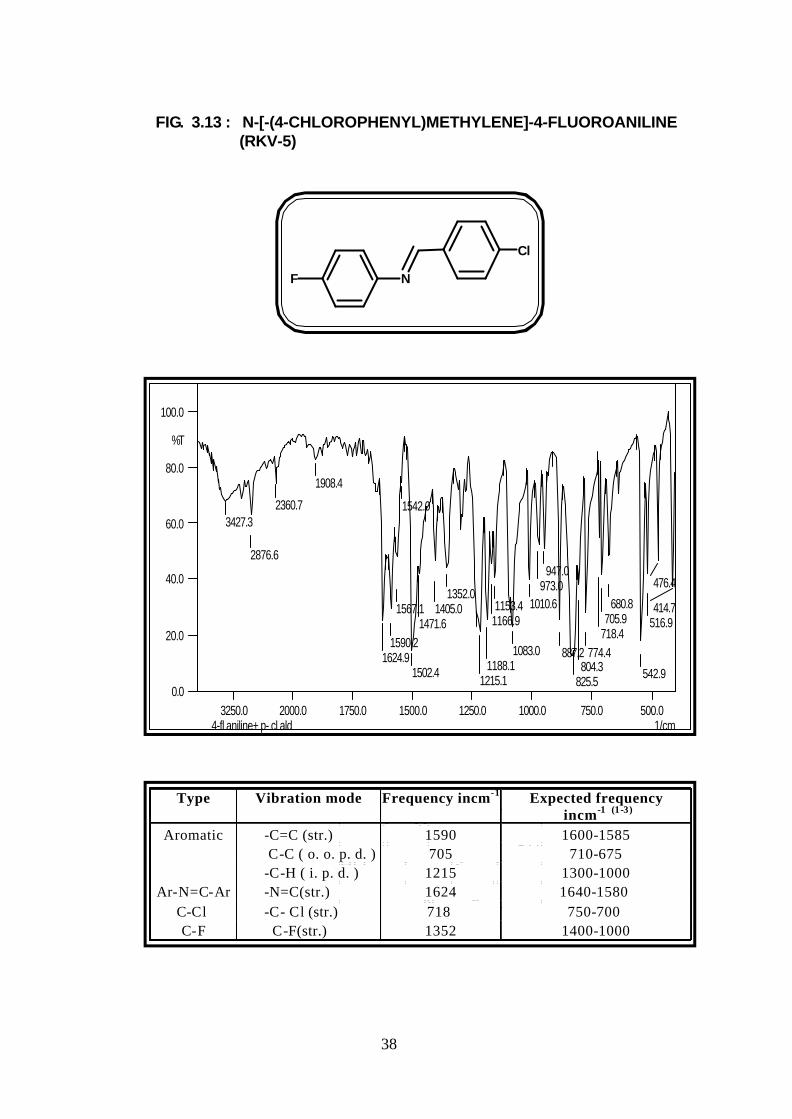
FIG. 3.13 : N-[-(4-CHLOROPHENYL)METHYLENE]-4-FLUOROANILINE (RKV-5)

NF

Cl

0.0

20.0

40.0

60.0

80.0

100.0

%T

500.0750.01000.01250.01500.01750.02000.03250.01/cm4-fl aniline+ p- cl ald

414.7

476.4

516.9

542.9

680.8 705.9

718.4 774.4

804.3 825.5

887.2

947.0 973.0

1010.6

1083.0

1153.41166.9

1188.11215.1

1352.01405.0

1471.6

1502.4

1542.0

1567.1

1590.21624.9

1908.4

2360.7

2876.6

3427.3

OH

N

HO

Type Vibration mode

Frequency incm-1

Expected frequency


C-C ( o. o. p. d. ) 705 710-675 -C-H ( i. p. d. ) 1215 1300-1000

Ar-N=C-Ar -N=C(str.) 1624 1640-1580 C-Cl -C- Cl (str.) 718 750-700 C-F C-F(str.) 1352 1400-1000

39

FIG. 3.14 : 4-[(4-FLUOROPHENYL)IMINO]METHYL-N,N-DIMETHYL- ANILINE (RKV-6)

NF

N

CH3

CH3

0.0

20.0

40.0

60.0

80.0

100.0

%T

500.0750.01000.01250.01500.01750.02000.03250.01/cm4-fl aniline+ n,n- di methyl ald poured

470.6

492.8

540.0

727.1

778.2

800.4

818.7

839.0

944.1 974.9

1066.6

1094.51123.5

1164.01216.0

1257.51293.2

1315.4

1365.5

1414.7

1429.2

1498.6

1530.4

1582.51604.7

2814.9

OH

N

H O

T y p e V i b r a t i o n m o d e

Frequency incm - 1


incm - 1 (1 -3 ) A l k a n e -C -H (str.) (sym.) 2 8 1 4 2 8 8 0 -2 8 6 0

-C -H(st r . ) (asym.) 2 9 6 0 2 9 7 5 -2 9 5 0 -N -( C H3 )2 1 3 6 5 1 3 8 5 -1 3 7 0

Aroma t i c -C = C - (str.) 1 5 8 3 1 6 0 0 -1 5 8 5 C -C ( o. o. p. d. ) 7 2 7 7 1 0 -6 7 5 -C -H ( i . p . d . ) 1 1 6 4 1 3 0 0 -1 0 0 0

A r-N = C - A r -N=C(s t r . ) 1 6 0 4 1 6 4 0 -1 5 8 0 C -F C -F(str .) 1 2 1 6 1 4 0 0 -1 0 0 0

40

FIG. 3.15 : 4-FLUORO-N-[-(4-METHOXYPHENYL)METHYLENE] ANILINE (RKV-7)

0.0

20.0

40.0

60.0

80.0

100.0

%T

500.0750.01000.01250.01500.01750.02000.03250.01/cm4-fl aniline+ p- anisaldehyde

420.5

435.9

487.0 512.1

542.9

580.5

725.2

748.3

787.9 810.0

840.9

886.2 974.0

1022.2

1096.51107.1

1160.1

1179.4

1209.31253.6

1279.7

1308.6

1360.7

1421.4

1440.7

1461.01498.6

1571.91603.7

1625.9

2845.83431.1

O H

N

H O




i n c m -1 ( 1 -3 )

A l k a n e -C -H ( s t r . ) ( s y m . ) 2 9 7 0 2 9 7 5 - 2 9 5 0 -C -H ( s t r . ) ( a s y m . ) 2 8 4 5 2 8 8 0 - 2 8 6 0 C -H ( b e n d ) 1 4 4 0 1 4 7 0 - 1 4 3 5

A r o m a t i c -C = C -( s t r . ) 1 6 0 3 1 6 0 0 - 1 5 8 5 C -C ( o . o . p . d . ) 7 2 5 7 1 0 - 6 7 5 -C -H ( i . p . d . ) 1 2 5 3 1 3 0 0 - 1 0 0 0

A r-N = C -A r -N = C ( s t r . ) 1 6 2 5 1 6 4 0- 1 5 8 0 C -F C -F ( s t r . ) 1 3 6 0 1 4 0 0 - 1 0 0 0

C -O -C C -O -C ( s t r . ) 1 0 2 2 1 0 7 0 - 1 0 0 0

NF

OCH3

41

FIG. 3.16 : 4-[(4-FLUOROPHENYL)IMINO]METHYL-2-METHOXYPHENOL (RKV-8)

NF

OH

OCH3

0.0

20.0

40.0

60.0

80.0

100.0

%T

500.0750.01000.01250.01500.01750.02000.03250.01/cm4-fl aniline+ vaniline

422.4

463.8 483.1 510.1

526.5

591.1

617.2

650.9

708.8

758.0

781.1

835.1

870.8 931.6

974.0

1028.01045.3

1092.6

1122.51159.11283.5

1380.0

1428.2

1463.9

1513.11593.1

1624.9

2848.7

2945.1

O H

N

H O




i n c m -1

- O - H - O - H ( s y m . ) 3 3 0 0 3 4 0 0 - 3 2 0 0 - O - H ( a s y m . ) 1 3 8 0 1 4 1 0 - 1 3 0 0

A l k a n e - C - H ( s t r . ) ( s y m . ) 2 8 4 9 2 8 8 0 - 2 8 6 0 - C - H ( s t r . ) ( a s y m . ) 2 9 4 5 2 9 7 5 - 2 9 5 0

A r o m a t i c - C = C - ( s tr . ) 1 5 9 3 1 6 0 0 - 1 5 8 5 C - C ( o . o . p . d . ) 7 0 8 7 1 0 - 6 7 5 - C - H ( i . p . d . ) 1 2 8 3 1 3 0 0 - 1 0 0 0

A r - N = C - A r - N = C ( s t r . ) 1 6 2 4 1 6 4 0 - 1 5 8 0 C - F C - F ( s t r . ) 1 1 5 9 1 4 0 0 - 1 0 0 0

C - O - C C - O - C ( s t r . ) 1 0 4 5 1 0 7 0 - 1 0 0 0

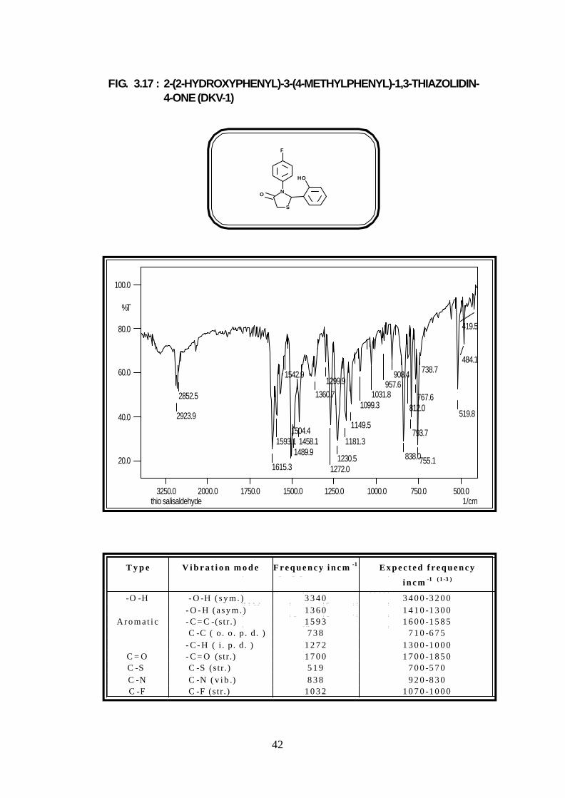
42

FIG. 3.17 : 2-(2-HYDROXYPHENYL)-3-(4-METHYLPHENYL)-1,3-THIAZOLIDIN- 4-ONE (DKV-1)

20.0

40.0

60.0

80.0

100.0

%T

500.0750.01000.01250.01500.01750.02000.03250.01/cmthio salisaldehyde

419.5

484.1

519.8

738.7

755.1

767.6

793.7

812.0

838.0

908.4 957.6

1031.81099.3

1149.5

1181.3

1230.51272.0

1299.91360.7

1458.11489.9

1504.4

1542.9

1593.1

1615.3

2852.5

2923.9

O H

N

H O


F r e q u e n c y i n c m -1


i n c m -1 ( 1 -3 )

-O -H - O -H ( s y m . ) 3 3 4 0 3 4 0 0 -3 2 0 0 - O - H ( a s y m . ) 1 3 6 0 1 4 1 0 -1 3 0 0

A r o m a t i c - C = C -(str . ) 1 5 9 3 1 6 0 0 -1 5 8 5 C -C ( o . o . p . d . ) 7 3 8 7 1 0 -6 7 5 - C - H ( i . p . d. ) 1 2 7 2 1 3 0 0 -1 0 0 0

C = O - C = O (str.) 1 7 0 0 1 7 0 0 -1 8 5 0 C -S C -S (str . ) 5 1 9 7 0 0 -5 7 0

C -N C -N ( v i b .) 8 3 8 9 2 0 -8 3 0 C -F C -F (str . ) 1 0 3 2 1 0 7 0 -1 0 0 0

F

N

S

O

OH

43

FIG. 3.18 : 2-(4-HYDROXYPHENYL)-3-(4-METHYLPHENYL)-1,3-THIAZOLIDIN- 4-ONE (DKV-2)

F

N

S

O OH

20.0

40.0

60.0

80.0

100.0

%T

500.0750.01000.01250.01500.01750.02000.03250.01/cm4-oh+thio

430.1

462.9 497.6

538.1 761.8

794.6

833.2

979.8

1103.2

1163.0

1188.1

1238.21286.4

1346.2

1388.7

1444.61502.4

1575.71598.9

1668.3

2327.9

2480.32590.2

3361.7

O H

N

H O




i n c m -1 (1 -3 )

-O -H - O - H ( s y m . ) 3 3 6 1 3 4 0 0 -3 2 0 0 - O - H ( a s y m . ) 1 3 8 8 1 4 1 0 -1 3 0 0

A r o m a t i c - C = C -(str . ) 1 5 9 8 1 6 0 0 -1 5 8 5 C -C ( o . o . p . d . ) 6 9 0 7 1 0 -6 7 5 - C - H ( i . p . d. ) 1 2 3 8 1 3 0 0 -1 0 0 0

C = O - C = O (str.) 1 6 6 8 1 7 0 0 -1 8 5 0 C -S C -S (str . ) 6 8 0 7 0 0 -5 7 0 C -N C -N ( v i b .) 8 3 3 9 2 0 -8 3 0 C -F C -F (str . ) 1 1 0 3 1 0 7 0 -1 0 0 0

44

FIG. 3.19: 3-(4-METHYLPHENYL)-2-(2-NITROPHENYL)-1,3-THIAZOLIDIN- 4-ONE (DKV-3)

F

N

S

O

O 2N

0.0

20.0

40.0

60.0

80.0

100.0

%T

500.0750.01000.01250.01500.01750.02000.03250.01/cmthio 2-no2

419.5

495.7

528.5 602.7

728.1

777.3

788.8

823.5

836.1

866.9

1133.11157.2

1219.91232.4

1301.9

1321.11349.1

1380.0

1449.4

1509.2

1604.7

1692.4

1869.82344.3

2852.5

2923.9

O H

N

H O




incm -1 (1 -3 )

A r o m a t i c - C = C -(str . ) 1 6 0 4 1 6 0 0 -1 5 8 5 C -C ( o . o . p . d . ) 7 2 8 7 1 0 -6 7 5 - C - H ( i . p . d . ) 1 2 3 2 1 3 0 0 -1 0 0 0

A r- N O 2 ( C - N O 2) ( sym.) 1 3 8 0 1 3 9 0 -1 2 5 0 ( C - N O 2) ( asym.) 1 5 0 9 1 5 9 0 -1 5 0 0

C = O C = O (str.) 1 6 9 2 1 8 5 0 -1 7 0 0 C -S C - S (str.) 6 0 2 7 0 0 -5 7 0 C -N C -N (vib . ) 8 3 6 9 2 0 -8 3 0 C -F C -F (str . ) 1 0 0 0 1 0 7 0 -1 0 0 0

45

FIG. 3.20: 2-(2-CHLOROPHENYL)-3-(4-METHYLPHENYL)-1,3-THIAZOLIDIN- 4-ONE (DKV-4)

F

N

S

O

Cl

0.0

20.0

40.0

60.0

80.0

100.0

%T

500.0750.01000.01250.01500.01750.02000.03250.01/cmthio o-cl

417.6 455.2

497.6

527.5

600.8 619.1

690.5

703.0

750.3

777.3

822.6

836.1

896.81015.5

1042.5

1096.51145.61156.2

1218.0

1234.4

1299.9

1320.21380.0

1449.41469.7

1509.2

1603.7

1692.4

2852.5

2924.8

O H

N

HO

Type Vibrat ion mode

Frequency incm -1

Expected frequency

incm -1 (1 -3 )

Aromatic -C=C-(str.) 1603 1600-1585 C-C ( o. o. p. d. ) 703 710-675 -C -H ( i. p. d. ) 1234 1300-1000

C =O C=O (str.) 1692 1850-1700 C-S C -S (str.) 600 700-570 C -N C-N (vib.) 836 920-830 C -C l C-Cltr.) 690 700-550 C-F C-F (str.) 1015 1070-1000

46

FIG. 3.21 : 2-(4-CHLOROPHENYL)-3-(4-METHYLPHENYL)-1,3-THIAZOLIDIN- 4-ONE (DKV-5)

30.0

40.0

50.0

60.0

70.0

80.0

90.0

100.0%T

500.0750.01000.01250.01500.01750.02000.03250.01/cmp-cl thio

432.0

493.7

580.5

613.3

761.8

815.8 835.1

1012.6

1087.8

1126.4

1159.11180.4

1213.1

1292.2

1334.6

1380.9

1413.7

1460.0

1508.2

1596.9

1681.8

3068.53446.6

O H

N

HO

Type Vibration mode

Frequency incm -1

Expected frequency

incm -1 (1 -3 )

Aromatic -C=C-(str.) 1596 1600-1585 C -C ( o. o. p. d. ) 680 710-675 -C -H ( i. p. d. ) 1213 1300-1000

C =O C = O (str.) 1681 1850-1700 C-S C -S (str.) 613 700-570 C -N C -N (vib.) 835 920-830 C -C l C -Cltr.) 580 700-550 C-F C -F (str.) 1012 1070-1000

F

N

S

O Cl

47

1H NMR Spectral data :

The study of radio frequency radiation by nuclear is called Nuclear Magnetic

Resonance (NMR).

1H NMR is one of the most powerful tools available to the chemists and

biochemists for elucidating the structure of chemical species.At a given radio

frequency, all protons in a molecule may give NMR at different applied field

strengths.

In the presence of an externally applied magnetic field, a spinning nucleus

can only assume a limited number of stable orientations. In a magnetic field, a

spinning nucleus in lower energetic orientation absorbs sufficient electromagnetic

radiation and is excited to a higher energetic orientation. This results in nuclear

magnetic resonance.

1H NMR spectrum gives valuable data about the carbon chain, structural

diagnosis, conformational analysis, determination of reaction velocities, keto-

enol tautomerism, to study exchange effects, in determination of activation energy,

decoupling experiments identify the neighboring groups of protons, paramagnetic

shift reagents simplify complex spectra, the adjacent groups of protons and also

the number of groups of equivalent protons and hence of the nature of atoms in

the chain, the integration give the number of protons in each group of equivalent

protons.

The NMR spectra were scanned on Burker 300 KHz by using deuterated

chloroform or dimethyl sulfoxide as a solvent.

The chemical shift (δ ppm), and multiplicities of some Schiff bases are

reported in Tables 3.1 to 3.14 along with their spectra. ( Figures: 3.22 to 3.35)

48

FIG

. 3.2

2 :

NM

R S

PE

CT

RA

OF

2-[

(4- H

YD

RO

XY

PH

EN

YL

) IM

INO

] ME

TH

YL

P

HE

NO

L (K

PV

-1)

49

Signal

No. Signal position

( δ ppm ) Relative No. Of Protons

Multiplicity

Inference

1 6.90 -8.23 8 H Multiple Ar - H 2 8.93 2 H Singlet = C - H

NOH

OH

TABLE 3.1 : NMR SPECTRAL STUDY OF 2-[(4- HYDROXYPHENYL) IMINO] METHYL PHENOL (KPV-1)

50

FIG

. 3.2

3 : N

MR

SP

EC

TR

A O

F 4

-[(

2-C

HL

OR

OP

HE

NY

L)

ME

TH

YL

EN

E]A

MIN

OP

HE

NO

L (

KP

V-2

)

51

Signal

No. Signal position


Multiplicity

Inference

a 6.86 -7.42 8 H Multiple Ar - H b 13.51 1 H Singlet O - H c 8.65 1 H Singlet = C - H

TABLE 3.2 : NMR SPECTRAL STUDY OF 4-[(2-CHLOROPHENYL) METHYLENE]AMINOPHENOL (KPV-2)

NOH

Cl

52

FIG

. 3.2

4 : N

MR

SP

EC

TR

A O

F 4

-[(

4-M

ET

HO

XY

PH

EN

YL

)ME

TH

YL

EN

E]A

MIN

OP

HE

NO

L (

KP

V-3)

53

TABLE 3.3 : NMR SPECTRAL STUDY OF 4-[(4-METHOXYPHENYL) METHYLENE]AMINOPHENOL ( KPV-3)

NOH

OCH3

Signal

No. Signal position


Multiplicity

Inference

a 6.83 -7.86 8 H Multiple Ar - H b 3.66 1 H Singlet O - H c 8.39 1 H Singlet = C - H d 3.89 3 H Singlet -OCH3

54

FIG

. 3.2

5 : N

MR

SP

EC

TR

A O

F 4

-[(

2-N

ITR

OP

HE

NY

L)M

ET

HY

LE

NE

]AM

INO

PH

EN

OL

(K

PV

-4)

55

TABLE 3.4 : NMR SPECTRAL STUDY OF 4-[(2-NITROPHENYL) METHYLENE]AMINOPHENOL (KPV-4)

HO N

O2N

Signal

No. Signal position


Multiplicity

Inference


56

FIG

. 3.2

6 : N

MR

SP

EC

TR

A O

F 4

-[(

3-N

ITR

OP

HE

NY

L)M

ET

HY

LE

NE

]AM

INO

P

HE

NO

L (

KP

V-5

)

57

TABLE 3.5 : NMR SPECTRAL STUDY OF 4-[(3-NITROPHENYL) METHYLENE]AMINO PHENOL (KPV-5)

NOH

NO2

Signal

No. Signal position


Multiplicity

Inference


58

FIG

. 3.2

7 : N

MR

SP

EC

TRA

OF

4-[

2-FU

RY

LME

THY

LEN

E]A

MIN

O P

HE

NO

L (K

PV-

6)

59

TABLE 3.6 : NMR SPECTRAL STUDY OF 4-[2-FURYLMETHYLENE]AMINO PHENOL (KPV-6)

NOHO

Signal

No. Signal position


Multiplicity

Inference

a 6.55 -7.44 4 H Multiple Ar - H

b 7.85 - 8.25 3 H Multiple - H (furaran) c 8.87 1 H Singlet = C - H

60

FIG

. 3.2

8 :

NM

R S

PE

CT

RA

OF

4-

[(4-

CH

OL

OR

OP

HE

NY

L)M

ET

HY

LE

NE

]AM

INO

PH

EN

OL

(K

PV

-7)

61

TABLE 3.7 : NMR SPECTRAL STUDY OF 4-[(4-CHOLOROPHENYL) METHYLENE]AMINOPHENOL (KPV-7)

NOH

Cl

Signal

No. Signal position


Multiplicity

Inference


62

FIG

. 3.2

9 : N

MR

SP

EC

TR

A O

F 4

-[(

4-H

YD

RO

XY

PH

EN

YL

)IM

INO

]ME

TH

YL

-2-

ME

TH

OX

YP

HE

NO

L (K

PV

-8)

63

TABLE 3.8 : NMR SPECTRAL STUDY OF 4-[(4-HYDROXY PHENYL) IMINO]METHYL-2-METHOXYPHENOL (KPV-8)

NOH

OH

OCH3

Signal

No. Signal position


Multiplicity

Inference

a 6.81 -7.62 7H Multiple Ar - H b 8.35 1 H Singlet = C - H c 8.95 1 H Singlet - O- H d 3.94 3H Singlet -OCH3

64

FI

G. 3

.30

: NM

R S

PE

CT

RA

OF

2-[

(4-F

LU

OR

OP

HE

NY

L) I

MIN

O]M

ET

HY

LP

HE

NO

L (

RK

V-1

)

65

TABLE 3.9 : NMR SPECTRAL STUDY OF 2-[(4-FLUOROPHENYL) IMINO]METHYLPHENOL (RKV-1)

NF

OH

Signal

No. Signal position


Multiplicity

Inference

a 6.91 -7.14 4 H Multiple Ar -OH

b 7.23 - 7.41 4 H Multiple Ar -F c 13.10 1 H Singlet -OH

d 8.59 1 H Singlet -N=CH

66

FIG

. 3.3

1 : N

MR

SP

EC

TRA

OF

4-FL

UO

RO

-N-(2

-NIT

RO

PH

EN

YL)

ME

THY

LEN

E]A

NIL

INE

(RK

V-3

)

67

TABLE 3.10 : NMR SPECTRAL STUDY OF 4-FLUORO-N-(2-NITROPHENYL) METHYLENE]ANILINE (RKV-3 )

NF

O2N

Signal

No. Signal position


Multiplicity

Inference

a 7.08 – 7.74 4 H Multiple Ar – NO2 b 8.06 – 8.31 4 H Singlet Ar - F c 8.93 1 H Singlet -N= C H

68

FIG

. 3.3

2 : N

MR

SP

EC

TR

A O

F N

-[-(

2-C

HL

OR

OP

HE

NY

L)

ME

TH

YL

EN

E]-

4-F

LU

OR

OA

NIL

INE

(R

KV-

4)

69

TABLE 3.11 : NMR SPECTRAL STUDY OF N-[-(2-CHLOROPHENYL) METHYLENE]-4-FLUOROANILINE (RKV-4)

NF

Cl

Signal

No. Signal position


Multiplicity

Inference

a 7.06 – 7.26 4 H Multiple Ar - F

b 7.35 – 8.24 4 H Singlet Ar – Cl c 8.90 1 H Singlet -N= C H

70

FIG

. 3.3

3 : N

MR

SP

EC

TR

A 2

-(2-

HY

DR

OX

YP

HE

NY

L)-3

-(4-

ME

THY

LPH

EN

YL)

-1,3

-TH

IAZO

LID

IN- 4

-ON

E (D

KV

-1)

71

TABLE 3.12 : NMR SPECTRAL STUDY OF 2-(2-HYDROXYPHENYL)-3- (4-METHYLPHENYL)-1,3-THIAZOLIDIN- 4-ONE (DKV-1)

F

N

S

O

OH

Signal

No. Signal position


Multiplicity

Inference

a 6.91 -7.14 4 H Multiple Ar - F b 7.23 - 7.40 4 H Multiple Ar -OH c 8.58 1 H Singlet -CH d 13.10 1 H Singlet - OH

72

FIG

. 3.3

4 : N

MR

SP

EC

TR

A O

F 3

-(4-

ME

TH

YL

PH

EN

YL

)-2-

(2-N

ITR

OP

HE

NY

L)-

1,3-

TH

IAZ

OL

IDIN

-4-O

NE

(D

KV-

3)

73

TABLE 3.13 : NMR SPECTRAL STUDY OF 3-(4-METHYLPHENYL)-2- (2-NITROPHENYL)-1,3-THIAZOLIDIN-4-ONE (DKV-3)

F

N

S

O

O2N

Signal

No. Signal position


Multiplicity

Inference

a 6.75 -7.32 4 H Multiple Ar - F

b 7.46 - 8.1 4 H Multiple Ar –NO2

c 3.74 - 3.92 2 H Singlet - CH2

d 2.9 - 3.0 1 H Singlet -CH

74

FIG

. 3.3

5 : N

MR

SP

EC

TR

A 2

-(2-

CH

LOR

OP

HE

NY

L)-3

- (4-

ME

THY

LPH

EN

YL)

-1,3

-TH

IAZO

LID

IN-4

-ON

E (

DK

V-4

)

75

TABLE 3.14 : NMR SPECTRAL STUDY OF 2-(2-CHLOROPHENYL)-3- (4-METHYLPHENYL)-1,3-THIAZOLIDIN-4-ONE (DKV-4)

F

N

S

O

Cl

Signal

No. Signal position


Multiplicity

Inference

a 6.51 -7.01 4 H Multiple Ar - F

b 7.19 - 7.36 4 H Multiple Ar –Cl c 3.79 - 3.96 2 H Multiple - CH2

76

Mass spectral analysis :

A molecule is fragmented with excess of energy from an electron in mass

spectrum. The probability of cleavage of a particular bond is related to the bond

strength and to the stability of the fragments.

The mass spectrum provides information about

> The elemental composition of samples of matter,

> The structure of inorganic, organic and biological molecules,

> The qualitative and quantitative composition of solid surfaces and

> Isotopic ratios of atoms in samples.

Further, it provides data which cannot be obtained from other spectra.For

example, information about the C-skeleton from fragment peaks, functional groups

from high m/z peaks and characteristic ion series, to distinguish between cis and

trans isomers, to study reaction mechanisms, to study biochemical reaction,

measurement of ionization potential of bond strengths, quantitative analysis of

mixtures, study of polymeric compounds etc.

In this technique, gaseous ions are separated according to their mass to

charge (m/z) ratio. A mass spectrum is plot of relative abundance of the gaseous

component as a function of the mass to charge (m/z) of the components.

The mass spectra of Schiff bases and thiazolidinones were taken on

[JEOL SX 102/DA-6000] and GCMS - SHIMADZU - QP2010 spectrometer and

are shown in Figures 3.36 to 3.56. The proposed fragmentation patterns are given

in schemes 1 to 21.

77

FIG

. 3.

36 :

MA

SS

SP

EC

TR

A O

F 2

-[(4

- HY

DR

OX

YP

HE

NY

L)I

MIN

O]M

ET

HY

LP

HE

NO

L (

KP

V-1

)

78

SC

HE

ME

3.1

: 2

-[(4

- HY

DR

OX

YP

HE

NY

L)I

MIN

O]M

ET

HY

LP

HE

NO

L (

KP

V-1

)

79

F

IG.

3.37

: M

AS

S S

PE

CT

RA

OF

4-[

(2-C

HL

OR

OP

HE

NY

L)M

ET

HY

LE

NE

]AM

INO

PH

EN

OL

(K

PV

-2)

80

SC

HE

ME

3.2

: 4

-[(

2-C

HL

OR

OP

HE

NY

L)M

ET

HY

LE

NE

]AM

INO

PH

EN

OL

(KP

V-2

)

81

FIG

. 3.

38 :

MA

SS

SP

EC

TR

A O

F 4-

[(4

-ME

TH

OX

Y P

HE

NY

L)M

ET

HY

LE

NE

]AM

INO

PH

EN

OL

( K

PV

-3)

82

SC

HE

ME

3.3

:

4-[

(4-M

ET

HO

XY

PH

EN

YL

)ME

TH

YL

EN

E] A

MIN

OP

HE

NO

L (

KP

V-3

)

83

FIG

. 3.

39 :

MA

SS

SP

EC

TR

A O

F 4-

[(2

-NIT

RO

PH

EN

YL

)ME

TH

YL

EN

E]A

MIN

OP

HE

NO

L (

KP

V-4

)

84

SC

HE

ME

3.4

: 4

-[(

2-N

ITR

OP

HE

NY

L)M

ET

HY

LE

NE

] AM

INO

PH

EN

OL

(KP

V-4

)

85

FIG

. 3.

40 :

MA

SS

SP

EC

TR

A O

F 4-

[(3

-NIT

RO

PH

EN

YL

)ME

TH

YL

EN

E]A

MIN

OP

HE

NO

L (K

PV

-5)

86

SC

HE

ME

3.5

: 4

-[(

3-N

ITR

OP

HE

NY

L)M

ET

HY

LE

NE

]AM

INO

PH

EN

OL

(KP

V-5

)

87

F

IG.

3.41

: M

AS

S S

PE

CT

RA

OF

4-

[2-F

UR

YL

ME

TH

YL

EN

E]A

MIN

OP

HE

NO

L (

KP

V-6

)

88

SC

HE

ME

3.6

: 4

-[2

-FU

RY

LM

ET

HY

LE

NE

]AM

INO

P

HE

NO

L (

KP

V-6

)

89

FIG

. 3.

42 :

MA

SS

SP

EC

TR

A O

F 4

-[(

4-C

HL

OR

OP

HE

NY

L)M

ET

HY

LE

NE

]AM

INO

PH

EN

OL

(KP

V-7

)

90

SC

HE

ME

3.7

: 4

-[(

4-C

HO

LO

RO

PH

EN

YL

)ME

TH

YL

EN

E] A

MIN

OP

HE

NO

L (

KP

V-7

)

91

FIG

. 3.

43 :

MA

SS

SP

EC

TR

A O

F 4-

[(4

-HY

DR

OX

Y P

HE

NY

L)I

MIN

O]M

ET

HY

L-

2-M

ET

HO

XY

PH

EN

OL

(K

PV

-8)

92

SC

HE

ME

3.8

: 4

-[(

4-H

YD

RO

XY

PH

EN

YL

)IM

INO

]ME

TH

YL

-2-

ME

TH

OX

YP

HE

NO

L (K

PV

-8)

93

FIG

. 3.

44 :

MA

SS

SP

EC

TR

A O

F 2

-[(4

-FL

UO

RO

PH

EN

YL

)IM

INO

]ME

TH

YL

PH

EN

OL

(RK

V-1

)

94

SC

HE

ME

3.9

: 2

-[(4

-FL

UO

RO

PH

EN

YL

)IM

INO

]ME

TH

YL

PH

EN

OL

(RK

V-1

)

95

FIG

. 3.

45 :

MA

SS

SP

EC

TR

A O

F 4

-[(4

-FL

UO

RO

PH

EN

YL

)IM

INO

]ME

TH

YL

PH

EN

OL

(RK

V-2

)

96

SC

HE

ME

3.1

0 :

4-[(

4-F

LU

OR

OP

HE

NY

L)I

MIN

O]M

ET

HY

LP

HE

NO

L (R

KV

-2)

97

FIG

. 3.

46 :

MA

SS

SP

EC

TRA

OF

4-F

LUO

RO

-N-[

-(2-

NIT

RO

PH

EN

YL)

ME

THY

LEN

E]A

NIL

INE

(RK

V-3

)

98

SC

HE

ME

3.1

1 : 4

-FL

UO

RO

-N-[

-(2-

NIT

RO

PH

EN

YL

)ME

TH

YL

EN

E]A

NIL

INE

(R

KV

-3)

99

FIG

. 3.

47 :

MA

SS

SP

EC

TR

A O

F N

-[-(

2-C

HL

OR

OP

HE

NY

L)M

ET

HY

LE

NE

]-4-

FL

UO

RO

AN

ILIN

E (R

KV

-4)

100

SC

HE

ME

3.1

2 :

N-[

-(2-

CH

LO

RO

PH

EN

YL

)ME

TH

YL

EN

E]-

4-F

LU

OR

OA

NIL

INE

(R

KV

-4)

101

FIG

. 3.

48 :

MA

SS

SP

EC

TR

A O

F N

-[-(

4-C

HL

OR

OP

HE

NY

L)M

ET

HY

LE

NE

]-4-

FL

UO

RO

AN

ILIN

E (R

KV

-5)

102

SC

HE

ME

3.1

3 : N

-[-(

4-C

HL

OR

OP

HE

NY

L)M

ET

HY

LE

NE

]-4-

FL

UO

RO

AN

ILIN

E (R

KV

-5)

103

FIG

. 3.

49 :

MA

SS

SP

EC

TR

A O

F 4

-[(4

-FL

UO

RO

PH

EN

YL

)IMIN

O]M

ET

HY

L-

N,N

-DIM

ET

HY

L- A

NIL

INE

(RK

V-6

)

104

SC

HE

ME

3.1

4 :

4-[

(4-F

LU

OR

OP

HE

NY

L)IM

INO

]ME

TH

YL

-N

,N-D

IME

TH

YL

- AN

ILIN

E (R

KV

-6)

105

FIG

. 3.

50 :

MA

SS

SP

EC

TR

A O

F 4

-FL

UO

RO

-N-[

(4-M

ET

HO

XY

PH

EN

YL

)ME

TH

YL

EN

E] A

NIL

INE

(RK

V-7

)

106

SC

HE

ME

3.1

5 :

4-F

LU

OR

O-N

-[-(

4-M

ET

HO

XY

PH

EN

YL

)ME

TH

YL

EN

E] A

NIL

INE

(R

KV

-7)

107

FIG

. 3.

51 :

MA

SS

SP

EC

TR

A O

F 4

-[(4

-FL

UO

RO

PH

EN

YL

)IM

INO

]ME

TH

YL

-2-

ME

TH

OX

YP

HE

NO

L (R

KV

-8)

108

SC

HE

ME

3. 1

6 :

4-[(

4-F

LU

OR

OP

HE

NY

L)I

MIN

O]M

ET

HY

L-

2-M

ET

HO

XY

PH

EN

OL

(R

KV

-8)

109

FIG

. 3.

52 :

MA

SS

SP

EC

TR

A O

F (2

-HY

DR

OX

YP

HE

NY

L)-

3-(4

-ME

TH

YL

PH

EN

YL

)-1,

3-T

HIA

ZO

LID

IN- 4

-ON

E (D

KV-

1)

110

SC

HE

ME

3.1

7 : -

(2-H

YD

RO

XY

PH

EN

YL

)-3-

(4-M

ET

HY

LP

HE

NY

L)-

1,3-

TH

IAZ

OL

IDIN

- 4-O

NE

(DK

V-1)

111

FIG

. 3.

53 :

MA

SS

SP

EC

TR

A O

F 2

-(4-

HY

DR

OX

YP

HE

NY

L)-

3-(4

-ME

TH

YL

PH

EN

YL

)-1,

3-T

HIA

ZO

LID

IN- 4

-ON

E (D

KV-

2)

112

SC

HE

ME

3.1

8 : 2

-(4-

HY

DR

OX

YP

HE

NY

L)-

3-(4

-ME

TH

YL

PH

EN

YL

)-1,

3-T

HIA

ZO

LID

IN-4

-ON

E (D

KV-

2)

113

FIG

. 3.

54 :

MA

SS

SP

EC

TR

A O

F 3

-(4-

ME

TH

YL

PH

EN

YL

)-2-

(2-N

ITR

OP

HE

NY

L)-

1,3-

TH

IAZ

OL

IDIN

- 4-O

NE

(DK

V-3)

114

SC

HE

ME

3.1

9 : 3

-(4-

ME

TH

YL

PH

EN

YL

)-2-

(2-N

ITR

OP

HE

NY

L)-

1,3-

TH

IAZ

OL

IDIN

-4-O

NE

(DK

V-3)

115

FIG

. 3.

55 :

MA

SS

SP

EC

TR

A O

F 2

-(2-

CH

LO

RO

PH

EN

YL

)-3-

(4-M

ET

HY

LP

HE

NY

L)-

1,3-

TH

IAZ

OL

IDIN

- 4-

ON

E (

DK

V-4

)

116

SC

HE

ME

3.2

0 : 2

-(2-

CH

LO

RO

PH

EN

YL

)-3-

(4-M

ET

HY

LP

HE

NY

L)-

1,3-

TH

IAZ

OL

IDIN

-4-O

NE

(D

KV-

4)

117

FIG

. 3.

56 :

MA

SS

SP

EC

TR

A O

F 2

-(4-

CH

LO

RO

PH

EN

YL

)-3-

(4-M

ET

HY

LP

HE

NY

L)-

1,3-

TH

IAZ

OL

IDIN

- 4-O

NE

(D

KV-

5)

SC

HE

ME

3.2

1 :

2-(4

-CH

LO

RO

PH

EN

YL

)-3-

(4-M

ET

HY

LP

HE

NY

L)-

1,3-

TH

IAZ

OL

IDIN

-4-O

NE

(DK

V-5)

119

References :

[1] V.M. Parikh, “Absorption Spectroscopy of Organic Molecules”,Addission

Wesley Pub., 243-258 (1978).

[2] D. L. Pavia, G.M. Lampan and G.S. Kriz, “Introduction of spectroscopy”,

Saunders Publishng, Philadelphia, 46 (1979).

[3] R. M. Silverstein, G.S. Basseleo, and T.C. Manrill ; “Spectroscopic

Identification of Organic Compounds”, 4th Edn., John Wiley and Sons,

York.75.

CHAPTER - IV

SECTION - 1

HEAT OF SOLUTION

120

Introduction :

The dissolution of a solute in a solvent is accompanied by the heat

change. If the heat is absorbed, i.e., the solution is cooler, the enthalpy change

(∆H) would be positive. If the heat is evolved, solution is warmer and so ∆H

would be negative. Thus, the heat of solution is defined as the change in

enthalpy, when one mole of substance is dissolved in specified quantity of

solvent at a given temperature. The molar heat of solution and melting

temperature of a substance can be determined from the solubility measurements

at different temperatures.

Literature survey shows that various workers studied thermodynamic

properties of several electrolytes in various pure and mixed solvents[1-8]. The heat

of solution for many organic and inorganic compounds, complexes, polymers etc.

have also been reported[9-19].

In the present work, heat of solution for the Schiff bases derived from

p-amino phenol was determined at 308.15 K in dimethylformamide (DMF) and

dimethylsulphoxide (DMSO).

121

Experimental :

The solvents used for the measurements were purified and fractionally

distilled prior to use by the method reported in the literature[20]. The solubility of

each Schiff base was determined by transferring 25 ml of saturated solution into

a pre-weighed 50 ml beaker at a definite temperature. The weight of beaker

along with solution was taken and the solvent was evaporated to dryness until

constant weight is obtained. This gives the weight of solute present in 25 ml

saturated solution. Three replicate measurements were carried out at a particular

temperature and average value of weight was determined. Subtraction of weight

of solute from the weight of solution gives the weight of solvent in 25 ml saturated

solution.

122

Results and Discussion:

The solubility (N2) of Schiff bases in both DMF and DMSO solvents are

given in Tables 4.1.1. It is observed that the solubility of Schiff bases is greater in

DMSO than in DMF. The dielectric constant (ε) of DMSO (ε = 46.6) is greater

than that of DMF (ε = 36.71). However, dipole moment of both the solvents,

DMSO and DMF are almost the same ( µ (DMSO) = 3.90 and µ (DMF) = 3.86).

Thus, dielectric constant of solvent plays an important role on the solubility of

studied Schiff bases.

In DMSO, the solubility is maximum for KPV-2 and minimum for KPV-5. In

DMF also, it is maximum for KPV-2 but minimum solubility is observed for KPV-1.

This suggests that the substituent groups also affect the solubility.

Further, Tables 4.1.1 shows that heat of solution are observed to be

positive for all the Schiff bases in both the solvents indicating thereby

endothermic behavior of these bases in both the solvents.

123

Table : 4.1.1 : The solubility and heat of solution of Schiff bases in DMF

and DMSO at 308.15 K.

DMF DMSO Compound code

N2 (.103 )

∆Hs (K.cal/mol)

N2 (.103 )

∆Hs (K.cal/mol)

KPV-1 0.0412 17.6899 0.0922 13.22557

KPV-2 0.0974 14.9156 0.1032 14.54788

KPV-3 0.0659 12.9253 0.0798 12.01739

KPV-4 0.0670 12.7806 0.0926 11.24671

KPV-5 0.0540 14.0998 0.0786 12.28948

KPV-6 0.0458 11.8315 0.0950 9.032239

KPV-7 0.0431 12.2403 0.0841 9.63699

KPV-8 0.0521 12.8982 0.0926 10.38911

124

References : [1] R. H. Wood and R. W. Smith, J. Phys. Chem., 69 (1965) 2974.

[2] R. H. Wood and H. L. Anderson, J. Phys. Chem., 70 (1966) 992.

[3] P. J. Reilly and R. H. Wood, J. Phys. Chem., 37 (1972) 3474.

[4] A. K. Shukla, J. C. Ahwalia and C. N. R, Rao, J. Chem. Soc., Faraday

Trans, 72 (1976) 1288.

[5] S. Ishiguro, B. Jeliazkova, H. Ohtaki, Bull. Chem. Soc. Jpn., 58 (1985)

1749.

[6] M. Khizkowsk, Fluid Phase Equi., 42 (1988) 269.

[7] S. Bhattacharyya, D. Rana and S. N. Bhattacharyya, J. Ind. Chem. Soc.,

74 (1997) 103.

[8] E. Matteoli and L. Lepori, Fluid Phase Equili., 174 (2000) 115.

[9] R. H. Wood, R. A. Rooney and J. N. Braddock, J. Phys. Chem., 73 (1969)

1673.

[10] I. R. Tasker, S. K. Suri and R. H. Wood, J. Chem. Eng. Data, 29 (1984)

193.

[11] D. G. Archer, H. J. Albert, D. E. White and R. H. Wood, J. Colloid Inter.

Sci., 100 (1984) 68.

[12] H. F. Holmes, R. H. Busey, J. M. Simonson, R. E. Mesmer, D. G. Archer

and R. H. wood, J. Chem. Thermodyn., 19, (1987) 863.

[13] N. U. Meurs, W. T. Warmerdam and G. Somsen, Fluid Phase Equi., 46

(1989) 263.

[14] P. H. Parsania, Asian J. Chem., 5 (1993) 312.

[15] E. S. Secco and R. A. Seccob, Phy. Chem. Chem. Phys., 1 (1999) 5011.

[16] A. W. Hakin, J. L. Liu, M. Shea and B. Zorzetti, Phys. Chem. Chem. Phys.,

4 (2003) 2653.

125

[17] J. M. Romero, L. C. Leiva, N. L. Jorge, M. E. Gomez Vara, E. A. Castro,

Acta Chim. Slov., 50, (2003) 579.

[18] S. Senkov, A. H. Roux and G. Roux-Desgranges, Phys. Chem. Chem.

Phys., 6 (2004) 822.

[19] O. Sklyar, T. H. Treutler, N. Vlachopoulos and G. Wittstock, Surface Sci.

597, (2005) 181.

[20] J. A. Riddick, W. B. Bunger, T. Sakano, “Organic Solvents-Physical

Properties and Methods for Purification”, 4th Edition, Vol.II, Wiley

Interscience, New York.

CHAPTER - IV

SECTION - 2

DENSITY

126

Introduction :

The measurement of density is useful in determining the purity of

substances. The determination of density of certain physiological liquids is

often an important screening tool in medical diagnosis.

Literature survey shows that much work has been done in liquid

mixtures [1-13] but scanty work has been reported for the solutions, which

include solutions of organic, inorganic and polymeric materials [14-27].

Thus, in the present chapter, the density of all the Schiff bases derived

from p-amino phenol are determined in dimethylformamide (DMF) and

dimethylsulfoxide (DMSO) solutions at 308.15 K.

127

Experimental:

The solvents DMF and DMSO were purified and fractionally distilled

prior to use [28].

All the Schiff bases were recrystallized from methanol. For each Schiff

base a series of solutions were prepared of different concentrations in both

the solvents. The density of all the solutions was measured by Pyknometer at

308.15 K. The results are given in Tables 4.2.1.

Results and Discussion : The density of solution (ρ12) is related to densities of the solvent, solute

and their weight fractions g1 and g2, according to the equation:

1/ρ12 = g1/ρ1 + g2/ρ2 ……….(4.2.1)

where ρ12 is density of solution and ρ1 and ρ2 are the densities of the solvent

and solute respectively. The obtained density results in Tables 4.2.1 are

related to a first order polynomial with respect to concentration in the following

form

ρ = a + bc ………..(4.2.2)

where ρ is density, c is concentration and a and b are coefficients of above

linear equation. The values of coefficients a and b and correlation coefficient

(γ) for all the Schiff bases are given in Table 4.2.2.

The calculated g1 and g2 values in DMF and DMSO solutions are

reported in Table 4.2.3 and 4.2.4 respectively. From the plot of 1/ρ12g1 verses

g2/g1, the density of Schiff bases were calculated. Figures 4.2.1 and 4.2.2

show the plots of 1/ρ12g1 verses g2/g1 in DMF and DMSO respectively. The

inverse of slope gives the density of Schiff base (ρ2). All these densities are

given in Table 4.2.5.

The density of a compound can also be determined theoretically by

following equation [29].

ρ = KM / NAΣ∆Vi ………. (4.2.3)

where ρ the density of the compound, K is is packing fraction (0.60), is the

molecular weight of the compound, NA is the Avogadro’s number and ∆Vi is

the volume increment of the atoms and atomic groups present in the

compound. ∆Vi for some of the atoms and group of atoms are given in Table

4.2.6. The densities calculated from equations (4.2.2) are given in Table 4.2.5.

129

It is observed from Table 4.2.5 that in some cases, there is quite good

agreement between theoretical and experimental density values where as in

others, deviations between theoretical and experimental densities are larger.

It is reported in section - 5 that in solutions, molecular interactions exist.

Usually intermolecular interactions do not affect the density but due to

polar substituent, there may be change in volume as well as in the molecular

weight of the compound. Thus, the deviations between experimental and

calculated values again confirm the existence of intermolecular interactions

between solute and solvent molecules.

130

Table 4.2.1: The density (ρ12) of Schiff bases in DMF and DMSO solutions at

308.15 K.

Density g * cm-3 Conc. ( M ) DMF

KPV-1 KPV-2 KPV-3 KPV-4 KPV-5 KPV-6 KPV-7 KPV-8

0.00 0.9356 0.9356 0.9356 0.9356 0.9356 0.9356 0.9356 0.9356

0.01 0.9366 0.9382 0.9380 0.9408 0.9382 0.9412 0.9373 0.9439

0.02 0.9378 0.9388 0.9404 0.9414 0.9403 0.9414 0.9397 0.9446

0.04 0.9386 0.9401 0.9429 0.9433 0.9412 0.9430 0.9431 0.9457

0.06 0.9396 0.9411 0.9444 0.9441 0.9422 0.9438 0.9441 0.9476

0.08 0.9405 0.9413 0.9452 0.9446 0.9444 0.9453 0.9479 0.9480

0.10 0.9413 0.9416 0.9472 0.9459 0.9482 0.9459 0.9498 0.9487

DMSO

0.00 1.0853 1.0853 1.0853 1.0853 1.0853 1.0853 1.0853 1.0853

0.01 1.0879 1.0887 1.0907 1.0926 1.0925 1.0940 1.0918 1.0928

0.02 1.0886 1.0890 1.0909 1.0930 1.0937 1.0946 1.0922 1.0935

0.04 1.0889 1.0893 1.0922 1.0937 1.0942 1.0949 1.0924 1.0954

0.06 1.0892 1.0899 1.0926 1.0945 1.0944 1.0956 1.0925 1.0957

0.08 1.0896 1.0901 1.0960 1.0963 1.0953 1.0969 1.0927 1.0962

0.10 1.0899 1.0912 1.0971 1.0976 1.0953 1.0971 1.0929 1.0965

131

Table 4.2.2 : Coefficients a and b obtained for DMF and DMSO solutions of

Schiff bases.

DMF Schiff bases

a b γ

KPV - 1 0.8205 1.0678 0.9982

KPV - 2 0.8890 1.0659 0.9963

KPV - 3 0.6288 1.0659 0.9738

KPV – 4 0.8234 1.0632 0.9971

KPV – 5 0.9245 1.0636 0.9493

KPV – 6 0.7487 1.0632 0.9975

KPV – 7 0.7496 1.0676 0.9598

KPV - 8 0.8208 1.0598 0.9967

DMSO

KPV - 1 0.8355 0.9191 0.9994

KPV - 2 0.8185 0.9188 0.9992

KPV - 3 0.6185 0.9179 0.9835

KPV – 4 0.7067 0.9160 0.9972

KPV – 5 0.8084 0.9151 0.9976

KPV – 6 0.7414 0.9143 0.9980

KPV – 7 0.8739 0.9159 0.9998

KPV - 8 0.7632 0.9150 0.9945

132

Table 4.2.3 : The weight fractions g1 and g2 of Schiff bases in DMF solutions at

308.15 K.

Conc. (M) g1 g2 g1 g2 g1 g2 g1 g2

KPV - 1 KPV - 2 KPV - 3 KPV - 4

0.01 0.9977 0.0023 0.9975 0.0025 0.9976 0.0024 0.9974 0.0026

0.02 0.9954 0.0046 0.9951 0.0049 0.9952 0.0048 0.9948 0.0052

0.04 0.9909 0.0091 0.9901 0.0099 0.9903 0.0097 0.9897 0.0103

0.06 0.9864 0.0136 0.9852 0.0148 0.9855 0.0145 0.9846 0.0154

0.08 0.9818 0.0182 0.9803 0.0197 0.9807 0.0193 0.9794 0.0206

0.10 0.9773 0.0227 0.9753 0.0247 0.9760 0.0240 0.9743 0.0257

KPV - 5 KPV - 6 KPV - 7 KPV - 8

0.01 0.9974 0.0026 0.9980 0.0020 0.9975 0.0025 0.9974 0.0026

0.02 0.9948 0.0052 0.9960 0.0040 0.9951 0.0049 0.9948 0.0052

0.04 0.9897 0.0103 0.9920 0.0080 0.9902 0.0099 0.9897 0.0103

0.06 0.9573 0.0427 0.9881 0.0119 0.9853 0.0148 0.9846 0.0154

0.08 0.9794 0.0206 0.9841 0.0159 0.9804 0.0196 0.9794 0.0206

0.10 0.9744 0.0256 0.9802 0.0198 0.9756 0.0244 0.9743 0.0257

133

Table 4.2.4 : The weight fractions g1 and g2 of Schiff bases in DMSO

Solutions at 308.15 K.

Conc. (M)

g1 g2 g1 g2 g1 g2 g1 g2

KPV - 1 KPV - 2 KPV - 3 KPV - 4

0.01 0.9980 0.0020 0.9979 0.0021 0.9979 0.0021 0.9978 0.0022

0.02 0.9960 0.0040 0.9957 0.0043 0.9958 0.0042 0.9956 0.0044

0.04 0.9920 0.0080 0.9915 0.0085 0.9917 0.0083 0.9911 0.0089

0.06 0.9880 0.0120 0.9872 0.0128 0.9875 0.0125 0.9867 0.0133

0.08 0.9840 0.0160 0.9830 0.0170 0.9834 0.0166 0.9823 0.0177

0.10 0.9800 0.0200 0.9787 0.0213 0.9792 0.0208 0.9779 0.0221

KPV - 5 KPV - 6 KPV - 7 KPV - 8

0.01 0.9978 0.0022 0.9983 0.0017 0.9979 0.0021 0.9978 0.0022

0.02 0.9956 0.0044 0.9966 0.0034 0.9957 0.0043 0.9955 0.0045

0.04 0.9911 0.0089 0.9932 0.0069 0.9915 0.0085 0.9911 0.0089

0.06 0.9867 0.0133 0.9898 0.0103 0.9873 0.0127 0.9867 0.0133

0.08 0.9823 0.0177 0.9863 0.0137 0.9830 0.0170 0.9822 0.0178

0.10 0.9779 0.0222 0.9829 0.0171 0.9788 0.0212 0.9778 0.0222

134

Fig. 4.2.1 : The plots of 1/ρ12g1 against g2/g1 for [A] KPV - 1 and [B] KPV - 2

in DMF at 308.15 K.

135

Fig. 4.2.2 : The plots of 1/ρ12g1 against g2/g1 for [A] KPV - 1 and [B] KPV - 2 in

DMSO at 308.15 K.

136

Table 4.2.5 : Experimental and calculated densities of Schiff bases in DMF

and DMSO solutions at 308.15 K.

Density gm/cm3 Solvents

Density gm/cm3

Compounds DMF

DMSO

Calculated from eqn. (4.2.3)

KPV - 1 1.3000 1.2727 1.1287

KPV - 2 1.1765 1.2000 1.1722

KPV - 3 1.6812 1.3572 1.1086

KPV - 4 1.2820 1.4285 1.1931

KPV - 5 1.5263 1.1800 1.1931

KPV - 6 1.5190 1.3530 1.3899

KPV - 7 1.2658 1.1210 1.1722

KPV - 8 1.2358 1.2000 1.0771

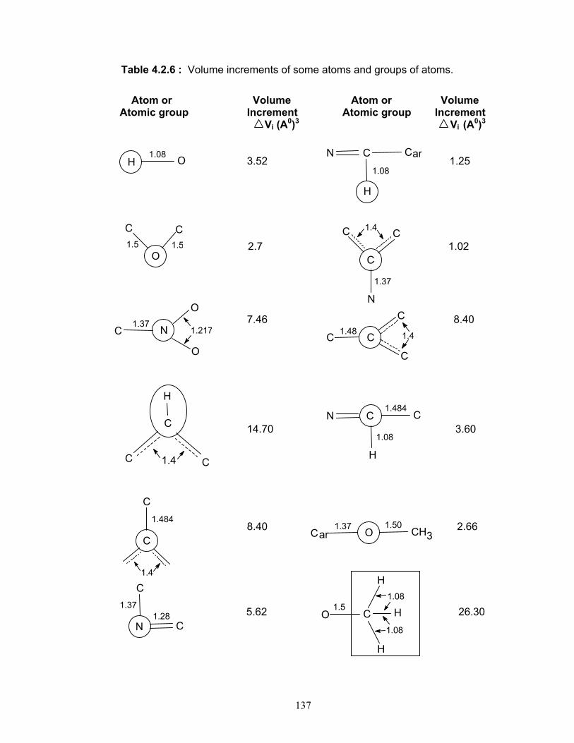
137

Table 4.2.6 : Volume increments of some atoms and groups of atoms.

Atom or Volume Atom or Volume Atomic group Increment Atomic group Increment Vi (A0)3 Vi (A0)3 3.52 1.25

2.7 1.02 7.46 8.40 14.70 3.60 8.40 2.66 5.62 26.30

1.08 OH

C

C

1.4

H

C

1.484

C

C

1.4

1.281.37

N C

C

1.4

C

C

1.37

N

C

1.41.48C C

C

C

N C C

H

1.08

1.484

1.37 CH31.50

C Oar

1.5 H

H

H

O C1.08

1.08

1.08

ar

H

CCN

1.5 1.5O

C C

O

O

NC1.37

1.217

138

Continue…(Table 4.2.6) Atom or Volume Atom or Volume Atomic group Increment Atomic group Increment Vi (A0)3 Vi (A0)3 11.65 5.6 10.10 7.84 19.35

12.641.48Car

O

C C 1.50

1.40

C1.27

O 7.29

C1.27

C 1.090.58

1.13

OC

CarC

ClCar1.77

1.37arC HO

1.08

1.4C C

C

C1.28

OC1.4

1.771.4 C Cl

C

139

References :

[1] W. J. Wallace, C. S. Shepherd and C. Underwood, J. Chem. Eng.

Data, 13 (1968) 11.

[2] A. J. Treszanowicz and G. C. Benson, J. Chem. Thermodyn., 9 (1977)

1189.

[3] J. Ortega and J. S. Matos, Mater. Chem. Phys., 15 (1986) 415.

[4] S. S. Joshi and T. M. Aminabhavi, Fluid Phase Equi., 60 (1990) 319.

[5] J. D. Pandey, P. Jain and V. Vyas, Can. J. Chem., 72 (1994) 63.

[6] A. Arce, J. M. Ageitos, J. Mendoza and A. Soto, J. Chem. Eng. Data,

41 (1996) 724.

[7] A. Pineiro, P. Brocos and A. Amigo, J. Chem. Thermodyn., 31 (1999)

931.

[8] R. Munoz, M. C. Burguet, V. M. Soria and R. N. de Arujo, Fluid Phase

Equi., 167 (2000) 99.

[9] A. Arce, J. M. Ageitos, E. Rodil and A. Soto, Fluid Phase Equi., 187

(2001)155.

[10] S. L. Oswal, R .L. Gardas and R. P. Phalak; Thermochimica Acta, 426

(2005) 199.

[11] S. Chen, Q. Lei and W. Fang, J. Chem. Eng. Data, 47 (2002) 811.

[12] R. Mehra, Ind. Acad. Sci., 115 (2003) 147.

[13] J. M. Resa et al. Fluid Phase Equilibria, , 217 (2004) 175.

[14] A. Tourino, M. Hervello, V. Moreno, G. Morino and M. Iglesias, J. Serb.

Chew.Soc., 69 (2004) 461.

[15] R. Sahai, V. Singh and R. verma, J. Ind. Chem. Soc., LIX (1982) 465.

[16] L. Oswal and M. V. Rathanam, Ind. J. Chem., 26A (1987) 29.

140

[17] T. M. Aminabhavi, M. I. Aralaguppi, B. Gopal Krishna and R. S.

Khinnavar, J. Chem. Eng. Data, 39 (1994) 52.

[18] A. Carton, F. Sobron, M. D. La Fuente and E. De Blas, J. Chem. Eng.

Data, 41 (1996) 74.

[19] E. Bottari and M. R. Festa. Springer J., 1 (1998) 22.

[20] R. Shukla and R. P. Mani, Asian J. Chem., 11 (1999) 584.

[21] J. Li, C. A. Prestidge and J. A. Mensah, J. Chem. Eng. Data, 45 (2000)

665.

[22] A. S. Burguate, P. B. Agarwal, S. W. Quazi and M. L. Narawade, Asian

J. Chem., 13 (2001) 1652.

[23] S. Chen, W. Fang, J. Yao and H. Zong, J. Chem. Eng. Data, 46 (2001)

596.

[24] D. C. Yin, Y. Inatomi, N. I. Waka, W. D. Huang, Cryst. Res. Technol.,

38 (2003) 785.

[25] N. A. Sanford, L. H. Robins, A. V. Davydov, A. Shpiro, D. V. Tsvetkov,

S. Keller, S. P. Denbeers, J. Appli. Phy., 94 (2003) 2095.

[26] C. E. Turner, D. A. Williamson, A. Paul and J. Talley, Int. Immo,

Pharm., 4 (2004) 1727.

[27] K. Zirk and H. Poetzschke, Med. Eng. Phy., 26 (2004) 473.

[28] J. A. Riddick, W. B. Bunger and Sakano, “Organic solvents physical

properties and Method of purification“. lVth edition, Techniques of

chemistry, 11, A Willey – Interscience publication John- Wiley.

[29] G. L. Slonimskii, A. A. Askadshii and A. I. Kitaigorodskii, Vysokomol,

Soyed, 12A (1970) 494.

CHAPTER - IV

SECTION - 3

CONDUCTANCE

141

Introduction:

Electrical conduction is a property of ionic solutions. The conductance of

electrolytic solutions depends on the concentration of the ions and also on the

nature of the ions present (through their charges and mobilities), and

conductance behavior as a function of concentration is different for strong and

weak electrolytes.

In physical chemistry, this technique is also used for determining the

ionization constant of weak electrolytes, in determining equilibrium constant and

rates of reactions that proceed with the formation or disappearance of ions, in

titration of solutions and in studies of interionic forces. Mullyniemi et al.[1] have

used an indirect conductometric screening method for the detection of antibiotic

residues in bovine kidneys. Sawai et al.[2] have used this technique to

investigate the growth of fungi. Literature survey shows that conductance of

many organic and inorganic compounds[3-17] have been measured in aqueous

and non-aqueous solvents, but very less data is available for Schiff bases and

their metal complexes[18-25]. Recently, conductances of some Schiff bases in

DMF and DMSO have been measured at different temperatures by Grzeszcuk

and Bator[26]. Further, in our laboratory, some conductance measurements have

been done for Schiff bases[27, 28].

The conductances of some Schiff bases of p-amino phenol are measured

in DMF and DMSO solutions at 308.15 K. The selection of these two solvents is

due to their dipolar aprotic characteristics, which avoid any proton interference

with the conductivity of complex systems[11]. The solubility restriction in media of

high dielectric constant does not allow for characterization of transport properties

in solvents of a wide range of varying dielectric constants.

142

Experimental : All the solvents used were distilled prior to use. The solutions of different

concentrations were prepared for each Schiff base in DMF and DMSO. The

conductance of each solution was measured by using Systronics Conductivity

Meter (Model No. 306) having cell constant 0.85 cm-1 at 308.15 K. The

conductance of each solution was corrected by subtracting conductance of pure

solvent.

143

Results and Discussion :

The measured conductance (C) for all the solution, after correction, was

used to determine the specific conductance κ, from which equivalent

conductance λC was calculated by the equation

κ = C θ ….. (4.3.1)

where θ is the cell constant.

λC = 1000 κ / c ..… (4.3.2)

where c is the concentration (g.equi/lit) of the solutions. The calculated values are

reported in Tables 4.3.1 and 4.3.2 for all Schiff bases derived from p-amino

phenol in DMF and DMSO at 308.15 K respectively. It is evident from Tables 4.3.1

and 4.3.2 that for all Schiff bases, equivalent conductance increases with dilution

in both the solvents. Further, It is observed that the values of λC are higher for

DMF than those in DMSO solutions. The equivalent conductance values

decreases in the following order :

In DMF : KPV-4 > KPV-2> KPV-3 > KPV-1 > KPV-5 > KPV-6 >KPV- 8 > KPV-7.

In DMSO : KPV-1 > KPV-7 >KPV-8 > KPV-2 > KPV- 6 > KPV-4 >KPV-5 > KPV-3.

It is observed that in DMF, the equivalent conductance of KPV- 4 is

maximum over the wide range of concentration whereas minimum λC is observed

in KPV-7. However, in DMSO, highest λC value is observed in KPV- 1 whereas

low λC is observed in KPV-3. This suggests that conducting behavior of Schiff

base depends on solvent and nature of solute under study rather than on its

molecular weight [12].

Due to different substituents present, conductance varies differently in

different solvents due to interaction between solute and solvent molecules. This is

explained in chapter-IV, section-5.

In DMF, presence of nitro group increases the equivalent conductance

whereas p-choloro substitution decreases the conductivity. However, in DMSO,

144

Table 4.3.1 The conductance (C) and equivalent conductance (λC) of Schiff bases in DMF at 308.15 K .

Conc. c

(gm/lit)

C. 105

(Ω)-1 λC

(cm2/Ω.equiv.)C. 105

(Ω)-1 λC


(Ω)-1 λC


(Ω)-1

λC (cm2/Ω.equiv.)

KPV - 1 KPV - 2 KPV - 3 KPV - 4 0.001 0.0500 0.4250 0.0585 0.4973 0.0549 0.4667 0.7100 6.0350 0.002 0.0610 0.2593 0.0653 0.2775 0.0574 0.2440 0.7470 3.1748 0.004 0.0780 0.1658 0.0749 0.1592 0.0616 0.1309 0.8010 1.7021 0.006 0.0960 0.1360 0.0833 0.1180 0.0647 0.0917 0.8420 1.1928 0.008 0.1260 0.1339 0.0906 0.0963 0.0679 0.0721 0.8850 0.9403 0.010 0.1550 0.1318 0.0969 0.0824 0.0699 0.0594 0.9210 0.7829 0.020 0.3000 0.1275 0.1310 0.0557 0.0800 0.0340 1.0900 0.4633 0.040 0.5310 0.1128 0.1850 0.0393 0.0800 0.0170 1.2000 0.2550 0.060 0.6300 0.0893 0.2130 0.0302 0.0833 0.0118 1.3900 0.1969 0.080 0.7330 0.0779 0.2250 0.0239 0.1320 0.0140 1.6000 0.1700 0.100 0.8590 0.0730 0.2390 0.0203 0.1350 0.0115 1.1700 0.0995

KPV - 5 KPV - 6 KPV - 7 KPV - 8 0.001 0.0504 0.4284 0.0181 0.1539 0.0088 0.0748 0.0110 0.0935 0.002 0.0652 0.2771 0.0247 0.1050 0.0111 0.0472 0.0144 0.0612 0.004 0.0678 0.1441 0.0381 0.0810 0.0149 0.0317 0.0200 0.0425 0.006 0.0694 0.0983 0.0492 0.0697 0.0181 0.0256 0.0232 0.0329 0.008 0.0717 0.0762 0.0594 0.0631 0.0214 0.0227 0.0268 0.0285 0.010 0.0731 0.0621 0.0673 0.0572 0.0237 0.0201 0.0355 0.0302 0.020 0.0828 0.0352 0.1040 0.0442 0.0374 0.0159 0.0565 0.0240 0.040 0.1000 0.0213 0.1538 0.0327 0.0623 0.0132 0.0941 0.0200 0.060 0.1190 0.0169 0.1821 0.0258 0.0794 0.0112 0.1180 0.0167 0.080 0.1300 0.0138 0.2124 0.0226 0.0991 0.0105 0.1530 0.0163 0.100 0.1410 0.0120 0.2500 0.0213 0.1160 0.0099 0.1900 0.0162

145

Table 4.3.2: The conductance (C) and equivalent conductance (λC) of Schiff bases in DMSO at 308.15 K.

Conc. c

(gm/lit)

C. 105

(Ω)-1 λC


(Ω)-1 λC


(Ω)-1 λC


(Ω)-1

λC (cm2/Ω.equiv.)

KPV - 1 KPV - 2 KPV - 3 KPV - 4 0.001 0.0760 0.6460 0.0323 0.2746 0.0152 0.1292 0.0230 0.1955 0.002 0.1310 0.5568 0.0674 0.2865 0.0178 0.0757 0.0295 0.1254 0.004 0.1860 0.3953 0.0839 0.1783 0.0242 0.0514 0.0421 0.0895 0.006 0.2340 0.3315 0.1050 0.1488 0.0263 0.0373 0.0434 0.0615 0.008 0.2480 0.2635 0.2160 0.2295 0.0314 0.0334 0.0452 0.0480 0.010 0.2580 0.2193 0.3320 0.2822 0.0357 0.0303 0.0475 0.0404 0.020 0.2610 0.1109 0.4280 0.1819 0.0477 0.0203 0.0519 0.0221 0.040 0.3480 0.0740 0.5860 0.1245 0.0808 0.0172 0.0777 0.0165 0.060 0.4110 0.0582 0.7340 0.1040 0.1090 0.0154 0.1050 0.0149 0.080 0.4860 0.0516 0.8790 0.0934 0.1440 0.0153 0.1310 0.0139 0.100 0.6320 0.0537 0.9150 0.0778 0.1660 0.0141 0.1550 0.0132

KPV - 5 KPV - 6 KPV - 7 KPV - 8 0.001 0.0240 0.2040 0.0260 0.2210 0.0596 0.5066 0.0395 0.3358 0.002 0.0271 0.1152 0.0333 0.1415 0.0760 0.3230 0.0424 0.1802 0.004 0.0332 0.0706 0.0454 0.0965 0.0842 0.1789 0.0486 0.1033 0.006 0.0366 0.0519 0.0569 0.0806 0.0901 0.1276 0.0539 0.0764 0.008 0.0423 0.0449 0.0682 0.0725 0.0995 0.1057 0.0590 0.0627 0.010 0.0438 0.0372 0.0704 0.0598 0.1060 0.0901 0.0617 0.0524 0.020 0.0465 0.0198 0.1080 0.0459 0.1160 0.0493 0.0876 0.0372 0.040 0.0580 0.0123 0.1930 0.0410 0.1620 0.0344 0.1260 0.0268 0.060 0.0676 0.0096 0.2820 0.0400 0.1670 0.0237 0.1660 0.0235 0.080 0.0728 0.0077 0.3490 0.0371 0.1740 0.0185 0.1920 0.0204 0.100 0.0810 0.0069 0.4250 0.0361 0.1920 0.0163 0.2310 0.0196

146

presence of –OH group increases while methoxy group decreases the equivalent

conductance.

The plots of equivalent conductance verses √c are given in Figure 4.3.1 in

both the solvents. It is clear from these figures that almost all Schiff bases are

weak electrolytes in nature.

For weak electrolytes, the equivalent conductance at infinite dilution (λ0)

can not be calculated by extrapolation of λC verses √c plots. However, we have

tried to determine λ0 values, by extrapolating these plots. These λ0 values are

given in Table 4.3.3. Singh et al[11] reported an alternative procedure to calculate

λ0 values for poly electrolytes. For the present systems, the same procedure was

tried to determine λ0 by the following equation:

κ = κ0 + λ0 c+ c φ(c) …………. (4.3.3)

where κ and κ0 are the electrolytic conductivities of the solutions and solvent

respectively. c is the equivalent concentration and the function φ(c) denotes the

effect of interionic interactions. The slope dκ/dc of the plot of κ verses c

approximates the limiting conductivity (λ0), provided other derivatives dκ0/dc and

d[cφ(c)]/dc in the differential form of equation (4.3.4) are neglected as compared

to λ0.

dκ/dc = dκ0/dc+ λ0 + d/dc [c φ(c)] ----- (4.3.4)

Figures 4.3.2 shows the variation of corrected conductance with

concentration for all Schiff bases in both DMF and DMSO at 308.15 K. It is clear

from the figures that in lower concentration range i.e., up to 0.01M, conductance

varies almost linearly with concentration for all the Schiff bases. However, non-

linearity is observed at higher concentration i.e. above 0.01M.

147

Figure 4.3.1: The plots of equivalent conductance verses √c for Schiff bases in

DMF and DMSO at 308.15 K.

DMF -KPV-1

0.0

0.3

0.6

0.0 0.2 0.4

C

equi

. con

d. (m

ho.c

m.2 /e

qui.)

DMSO -KPV-1

0.0

0.4

0.8

0.0 0.2 0.4

C

equi

. con

d. (m

ho.c

m.2 /e

qui.)

DMF-KPV-2

0.0

0.3

0.6

0.0 0.2 0.4

C

equi

. con

d. (m

ho.c

m.2 /e

qui.)

DMSO-KPV-2

0.00

0.15

0.30

0.0 0.2 0.4

C

equi

. con

d. (m

ho.c

m.2 /e

qui.)

DMF-KPV-3

0.0

0.3

0.6

0.0 0.2 0.4

C

equi

. con

d. (m

ho.c

m.2 /e

qui.)

DMSO-KPV-3

0.00

0.08

0.16

0.0 0.2 0.4

C

equi

. con

d. (m

ho.c

m.2 /e

qui.)

148

Figure 4.3.1: (contd.)…..

DMF-KPV-4

0

4

8

0.0 0.2 0.4

C

equi

. con

d. (m

ho.c

m.2 /e

qui.)

DMSO-KPV-4

0.00

0.12

0.24

0.0 0.2 0.4

C

equi

. con

d. (m

ho.c

m.2 /e

qui.)

DMF-KPV-5

0.0

0.3

0.6

0.0 0.2 0.4

C

equi

. con

d. (m

ho.c

m.2 /e

qui.)

DMSO-KPV-5

0.00

0.12

0.24

0.0 0.2 0.4

C

equi

. con

d. (m

ho.c

m.2 /e

qui.)

DMF-KPV-6

0.00

0.10

0.20

0.0 0.2 0.4

C

equi

. con

d. (m

ho.c

m.2 /e

qui.)

DMSO-KPV-6

0.00

0.12

0.24

0.0 0.2 0.4

C

equi

. con

d. (m

ho.c

m.2 /e

qui.)

149


DMF-KPV-7

0.00

0.04

0.08

0.0 0.2 0.4

C

equi

. con

d. (m

ho.c

m.2 /e

qui.)

DMSO-KPV-7

0.0

0.3

0.6

0.0 0.2 0.4

C

equi

. con

d. (m

ho.c

m.2 /e

qui.)

DMF-KPV-8

0.00

0.06

0.12

0.0 0.2 0.4

C

equi

. con

d. (m

ho.c

m.2 /e

qui.)

DMSO-KPV-8

0.0

0.2

0.4

0.0 0.2 0.4

C

equi

. con

d. (m

ho.c

m.2 /e

qui.)

150

Figure 4.3.2: Variation of conductance with concentration for Schiff bases in

DMF and DMSO at 308.15 K.

DMF -KPV-1

0.0

0.5

1.0

0.00 0.06 0.12

Concentration (M)

Con

duct

ance

. 10

5 (mho

) DMSO -KPV-1

0.0

0.5

1.0

0.00 0.06 0.12

Concentration (M)

cond

ucta

nce

. 105 (m

ho)

DMF-KPV-2

0.0

0.2

0.4

0.00 0.06 0.12

Concentration (M)

Con

duct

ance

. 10

5 (mho

)

DMSO-KPV-2

0.0

0.5

1.0

0.00 0.06 0.12

Concentration (M)

cond

ucta

nce

. 105 (m

ho)

DMF-KPV-3

0.00

0.08

0.16

0.00 0.06 0.12

Concentration (M)

cond

ucta

nce

. 105 (m

ho)

DMSO-KPV-3

0.00

0.10

0.20

0.00 0.06 0.12

Concentration (M)

cond

ucta

nce

. 105 (m

ho)

151


DMF-KPV-4

0.0

1.0

2.0

0.00 0.06 0.12

Concentration (M)

con

dduc

tanc

e . 1

05 (mho

)

DMSO-KPV-4

0.00

0.10

0.20

0.00 0.06 0.12

Concentration (M)

cond

ucta

nce

. 105 (m

ho)

DMF-KPV-5

0.00

0.08

0.16

0.00 0.06 0.12

Concentration (M)

cond

ucta

nce

. 105 (m

ho)

DMSO-KPV-5

0.00

0.05

0.10

0.00 0.06 0.12

Concentration (M)

cond

ucta

nce

. 105 (m

ho)

DMF-KPV-6

0.00

0.12

0.24

0.00 0.06 0.12

Concentration (M)

con

duct

ance

. 10

5 (mho

)

DMSO-KPV-6

0.0

0.3

0.6

0.00 0.06 0.12

Concentration (M)

cond

ucta

nce

. 105 (m

ho)

152


DMF-KPV-7

0.00

0.06

0.12

0.00 0.06 0.12

Concentration (M)

cond

ucat

nce

. 105 (m

ho)

DMSO-KPV-7

0.00

0.10

0.20

0.00 0.06 0.12

Concentration (M)

cond

ucta

nce

. 105 (m

ho)

DMF-KPV-8

0.00

0.08

0.16

0.00 0.06 0.12

Concentration (M)

con

duct

ance

. 10

5 (mho

)

DMSO-KPV-8

0.00

0.12

0.24

0.00 0.06 0.12

Concentration (M)

cond

ucta

nce

. 105 (m

ho)

153

As interionic interactions are present in all the systems over the wide

range of concentrations, so the derivative d[cφ(c)]/dc cannot be ignored in

comparison to λ0. However, limiting equivalent conductivities were evaluated

from the limiting slope of small linear portions of the κ verses c curve, assuming

that the interionic interactions in this range of concentration are limited. For all

the systems, the calculated λ0 values are given in Table 4.3.3. It is evident from

Table 4.3.3 that except for KPV - 5 and KPV - 8 in DMF, deviations are quite high

between the values evaluated from graph and those calculated by eq. 4.3.3. This

suggests that for the studied Schiff bases, eq. ( 4.3.3 ) is not valid.

154

Table 4.3.3: The limiting equivalent conductance (λ0) for all Schiff bases in DMF and

DMSO at 308.15 K.

DMF DMSO Compound

Code λo

( cm2/Ωequiv.)

λo

( cm2/Ωequiv.)

calc. by eq. (4.3.2)

λo

( cm2/Ωequiv.)

λo

( cm2/Ωequiv.)

calc. by eq. (4.3.2)

KPV - 1

KPV - 2

KPV - 3

KPV - 4

KPV - 5

KPV - 6

KPV - 7

KPV - 8

8.18

3.91

1.40

22.50

1.25

5.24

1.60

0.27

0.70

0.95

0.75

13.70

1.30

0.33

0.15

0.19

2.50

1.61

2.24

1.07

2.43

5.86

3.75

2.71

0.86

0.38

0.22

0.32

0.45

0.40

1.10

0.78

155

References: [1] A. L. Myllyniemi, H. Sipla, L. Nuotio, A. Niemi and T. Honkanen-Buzalski,

Analyst, 127 (2002) 1247.

[2] J. Sawai and T. Yoshikawa, Lett. Appl. Microbiol., 37 (2003) 40.

[3] J. M. Notley and M. Spiro, J. Phys. Chem., 70 (1966) 1502.

[4] R. Wachter and J. Barthel, Ber. Bunsenges. Phys. Chem., 83 (1979) 634.

[5] A. N. Singh, Ind. J. Chem. Sec. A, 19 A (1981) 1215.

[6] H. G. Mukherjee and S. K. Datta, J. Ind. Chem. Soc., LXII (1985) 67.

[7] K. Daga, S. Gaur, S. P. Ranga and R. K. Mehta, J. Ind. Chem. Soc., LXV

(1988) 79.

[8] V. Voitylov, S. Kakorin and A. Trusov, Colloid. J., 52 (1990) 15.

[9] O. Bernard, W. Kunz, P. Turq and L. Blum, J. Phys. Chem., 96 (1992)

398.

[10] G. P. Goshi, D. A. Wasylyshyn and S. K. Jain, J. Chem. Soc. Faraday

Trans., 90 (1994) 2065.

[11] M. Singh, A. Kumar, S. Easo and B. B. Prasad, Can. J. Chem., 75 (1997)

414.

[12] M. Hasani and A. Afkhani, Asian. J. Chem., 12 (2000) 712.

[13] M. Tomsic, M. B. Rogac, A. Jamnik, R. Neueder and J. Barthel, J. Sol.

Chem., 31 (2002) 19.

[14] B. P. Dey, P. K. Biswas and S. C. Lahiri, J. Ind. Chem. Soc., 80 (2003)

271.

[15] P. Haldar and B. Das, Z. Phy. Chem., 218 (2004) 1129.

[16] M. G. Abd,S. E. Wanes, M. Gamel and S. Haleem, J. Serb. Chem. Soc., 69 (2004) 183.

156

[17] M. B. Rogac, V. Babic, T. M. Perger, R. Neueder and J. Barthel, J. Mol.

Liqds, 118 (2005) 111.

[18] V. V. Popok, Colloids and Surfaces, 250 (2004) 467.

[19] M. Hrudananda and K. C. Das, J. Inorg. Nucl. Chem., 39 (1977) 1345.

[20] L. D. Dave and K. Ammae, J. Ind. Chem. Soc., LXII (1985) 178.

[21] S. R. R. Thomas and G. Parameswaram, J. Ind. Chem. Soc., 69 (1992)

117.

[22] C. Singh, H. K. Parwana, G. Singh and R. S. Jolly, Asian J. Chem., 12

(2000) 1.

[23] J. Hong, F. X. Xie, X. S. Sheng and X. Dazhao, Asian J. Chem., 14 (2002)

821.

[24]. T. B. S. A. Ravoof, K. A. Crouse, M. Ibrahim, M. Tahir, A. R. Cowleyand

and M. A. Ali, Polyhedron, 23 (2004) 2491.

[25] S. Chandra and L. K. Gupta, Spectrochim. Acta, Part A, Mol. Boimol.

Spectroscopy, 62 (2005) 307.

[26] M.Grzeszcuk and G.Bator, Polish J.Chem., 76 (2002) 1143.

[27] S. Baluja, E.J.Chem., 01 (2004).

[28] S. Baluja, Acta Ciencia. Indica., XXX (2004) 163.

CHAPTER - IV

SECTION - 4

DISSOCIATION CONSTANT

157

Introduction :

The dissociation constants are used to measure the strength of acid

and bases. They are also known as acidity constant, ionization constant or

formation constant.

Since long chemists have concerned themselves with the development

of precise methods of measuring acidity constants. In general terms, any

physical property, which varies with protonation, may provide a suitable

method for the measurement of dissociation constants.

The dissociation or acidity constant is determined by determining one

of the species, at equilibrium. The activity or concentration of the others can

be calculated from the amount of the acid or base initially introduced and the

stoichiometry of the acid base equilibrium. As the equilibrium is highly mobile,

physical methods, which do not disturb the equilibrium, are preferred for the

determination of the equilibrium concentration of the species present. For the

measurement of dissociation constant, various methods have been

developed [1], such as: (i) potentiometry including pH metry, (ii) spectrophoto-

metry, (iii) conductometry, (iv) solubility measurements[1], (v) cryoscopy[2],

(vi) measurement of the relative distribution of an acid between two immiscible

solvents[3], (vii) measurements of the rates of acid catalyzed hydrolysis of

esters[4], (viii) magnetic measurements etc. Recently, some new methods

such as capillary electrophoresis[5-7], Ikuta and Hirokawa[8] , feedback-based

flow ratiometry[8,9], UV visible[10] , mass spectrometry[11] etc. have also been

used to determine acid dissociation constant. The use of Raman spectra and

nuclear magnetic constants are also known to be used for a number of acids,

which are regarded as strong in aqueous solution [10, 12, 13].

For very week acids, conductance method was used, which was more

time consuming[4]. When the acid is sparingly soluble and acid strengths are

very high or very low. Spectrophotometer method is considered to be an ideal

method, but this method is also more time consuming. It is applicable if at

least one of the species at equilibrium absorbs characteristically in the

ultraviolet or visible region and the relevant ionic species show absorption

maxima at different wavelengths.

158

The most time economical method is potentiometry, which is mostly used

for the determination of dissociation constants of acids. Further, it can be used

for acids of pKa range from 2 to 11 units[12]. The calomel and glass electrodes

are used for the measurement[4] and carbonate free potassium hydroxide is the

best alkali to use as a titrant.

The potential generated by the hydrogen ions, in the solution of an acid in

a given medium is measured by an electronic potentiometer assembly. The

relationship between the potential of glass electrode and the pH of the solution

has the general form:

-log [H+] = pH = E0 – Ec / 0.0591 at 250C

where E0 is the observed potential and Ec is the potential of the calomel

electrode. All these terms in above equation change with time. So, it must be

calibrated before and after use with a pair of known buffers, the pH of one of

which must lie near to the pH region to be measured. The correctness of the

results depends upon the exactness of the calibration of pH-meter. The

reference solutions of known pH are preferred due to three primary reasons [14].

1. Saturated calomel reference electrodes are not highly reproducible

and this is particularly true for small immersion type electrode.

2. The potentials of the commercial glass electrodes vary widely and the

symmetry potentials may fluctuate from day to day.

3. The pH meter is usually calibrated to read directly in pH units.

Accurate results cannot be expected if pKa to be determined is very low.

In such cases, more sensitive instruments should be used.

The pH metric methods measure directly the activity of the hydrogen

ions. So, one can get reliable values of dissociation constant by this method.

This method is very popular although there are certain difficulties in mixed

aqueous media and non-aqueous media. The solubility method for determining

pKa is not so accurate as conductometric, potentiometric or spectrophotometric

technique, but is useful in cases where the substance is too insoluble in water

for conductometric or potentiometric methods.

159

There are many applications of dissociation constants. The nature of

the functional groups can be determined by simple comparison of acidity or

dissociation constant of the unknown compound with those of known

compounds. The dissociation or formation constant also provides useful

information about structure, tautomeric equilibria, solvent-solute interactions

etc.[15]. By determining dissociation constants, Prenesti et al. interpreted acid–

base properties of grape red wines [16].

Generally, the formation constant and other thermodynamic properties

of water-insoluble compounds are measured in purely non-aqueous organic

solvent or in a mixture of two solvents, one of which may be water. A solvent

mixture containing water and water-miscible organic solvent is known as mixed

aqueous medium. A number of works has been done in non-aqueous and

mixed-aqueous media [17-23].

Various workers studied the dissociation constant of many

substances[24-28] by using different methods. Grunwald[29] measured ionization

of formic acetic and benzoic acid by differential potentiometry. Czaja et al also

used this technique for the determination of dissociation constant of substituted

phenols[30]. Sandhu[31] used pH metry for the determination of stability

constants of some complexes.

The ionization constants of various other acids in pure and mixed

solvents have also been studied [32-39].

Pardeshi and Bhobe reported dissociation constants of some amino

acids[40]. Arora et al[41]., reported the dissociation constant of some hydroxyl

coumarins in ethanol-water mixtures. Etxebarria et al. determined the

protonation constant of 4-methylpyridine in potassium nitrate-toluene

systems[42]. Palanichamy[43] studied the dissociation constants of some

aliphatic acids and amino acids by potentiometry. Rengaraj et al. and others

determined formation constant of some Schiff bases and their metal

complexes[44]. Robert et al.[45] reported the acidity constants of benzidine and

N,N-dimethylbenzidine. Boraei and Ahmed[46] studied formation constant of

transition metal ion mixed complexes of tricine and 8-hydroxy quinoline.

A computer programme was also reported to determine conditional

formation constant of carbonic acid in sea water[47]. Ghaseni et al[48] studied

160

the acidity constant of 4-(2-pyridylazo)resorcinol in acetonitrile-water mixtures.

The dissociation constant of some biologically active sulfonamides have also

been reported by Remko and Lieth[49]. Partanen and Covington reported the

dissociation constants from electrochemical cell data for propionic acid and n-

butyric acids and some aliphatic carboxylic acids in aqueous sodium chloride

solutions[50].

In the present work, the dissociation constants of some Schiff bases

are studied in 1, 4- dioxane-water (60:40 v/v) mixture at 308.15 K.

161

Experimental :

The chemicals used were of B.D.H Analar grade. All solutions used for

the titration are prepared using distilled water. Following are the

concentrations of the solutions used for the titration.

Solutions Concentration (M) Nitric acid 0.1

Sodium hydroxide 0.5, 0.1

Sodium nitrate 1.0

Schiff base (in 1,4-dioxane) 0.1

Nitric acid and sodium hydroxide were standardized by titrating with

0.1 N NaOH and 0.05 M succinic acid solution respectively.

The 1, 4-dioxane used was of S. Merck and was purified by the reported

method [51].

The buffer solutions used for the calibration of pH meter were 0.05 M

potassium hydrogen phthalate and 0.01 M Borax buffer.

A systronic pH meter (Model No. EQ 664) was used for the pH

determination. The systronic glass electrode and a saturated calomel

electrode were used as indicator and reference electrodes respectively.

Before operation, the glass electrode was immersed in 0.1 M HCl for twenty

minutes. Then, it was washed thoroughly with distilled water.

Before measurement, the pH meter was calibrated with buffer solution of

known pH.

162

Calvin Bjerrum pH titration :

The following sets of mixtures were prepared for titration:

(I) 0.8 ml HNO3 (0.1M) + 11.2 ml water + 24.0 ml 1, 4-dioxane + 4.0 ml

NaNO3 (1.0 M).

(ii) 0.8 ml HNO3 (0.1M) + 11.2 ml water + 22.0 ml 1, 4-dioxane + 2.0 ml

ligand solution (0.1M) + 4.0 ml NaNO3 (1.0 M).

Thus, total volumes (V0) in each set = 40.0 ml and 1, 4-dioxane: water

ratio 60:40 (v/v).

The above mentioned solutions were allowed to attain a constant

temperature (308.15 K) and then titrated against standard NaOH solution (0.5

M) under an inert atmosphere of nitrogen. The change in the pH of solution

with each addition of alkali was recorded and is given in Tables 4.4.1.

163

Theory :

In the present work, except KPV-1, other Schiff bases are of HL type.

KPV-1 is of H2L type. Thus, the equilibria are,

L + H ↔ HL

and

L + H ↔ HL

H L + H ↔ H2L

In general, these equations can be represented as:

The thermodynamic proton-ligand stability constant (TKjH ) is given by:

[ ] 1

jHj

j

LHTK

LH H−

=

……….. (4.4.1)

TKjH is reciprocal of the thermodynamic dissociation constant of the acid LHj

dissociating as:

The overall thermodynamic proton-ligand stability constant βjH is given by:

[ ][ ]

jHj j

LHT

L Hβ

= ……….. (4.4.2)

and it refers to the reaction:

The stoichiometric proton-ligand stability constant is given by:

[ ] 1

jHj

j

LHK

LH H−

=

……….. (4.4.3)

and

[ ][ ]

jHj j

LH

L Hβ

= ……….. (4.4.4)

164

An inert electrolyte is used to determine the stability constant in a

particular salt medium. Sodium nitrate is mostly preferred as supporting

electrolyte, because of very slight complexing tendency of nitrate ion.

Generally, the competition between nitrate ion and the ligand under study is

minor importance. The molar concentrations are used in place of activities.

For the determination of dissociation constants, Bjerrum[52] introduced a

relation for the determination of Hn , which is defined as average number of

hydrogen bound to each ligand.

Hn = K1H [H] + 2K1

H K2H [H]2 + .....JK1

H K2H [H] ... Kj

H [H]j / 1 + K1H [H] + K1

H

K2H [H]2.....K1

HK2H.....Kj

H [H]j …….......(4.4.5)

From equation (4.4.4), we can write

[ ]

[ ]1

1

jHj

jH

jHj

j

j Hn

H

η

η

β

β

=

=

=∑

∑ : ( )0 1Hβ = ………… (4.4.6)

Equation (4.4.6) is called Bjerrum formation function of the system.

The determination of dissociation or formation constants from

experimental data comprises the following three steps: (i) evaluation of

formation curve of the system (ii) calculation of stoichiometric K`s of the

system by direct solution of the formation function and (iii) conversion of

stoichiometric constants into thermodynamic constants.

When the system consists of a ligand, which is a conjugated base of a

weak acid, the pH-metric method introduced by Bjerrum [52] has been widely

used. This method is known as "Bjerrum-Calvin pH titration technique".

In this technique, concentration of H+ ions is measured potentiometrically.

Thus, a large amount of data can be obtained in a short period of time. The

Irving and Rossotti method [53] has some advantages, such as:

(i) This method is valid for both pure water and for the mixed solvents.

(ii) In this method, it is not necessary to convert the pH-meter reading in to

stoichiometric hydrogen ion concentration.

165

(iii) It is not necessary to know the stoichiometric concentration of neutral

salt added to maintain the ionic strength constant.

Due to these advantages, this method is used in the present work.

In this method, the pH-meter is standardized using an aqueous buffer

and the meter reading B is plotted against volume of alkali used to titrate:

(1) A mixture containing a mineral acid, a chelating agent and a neutral

electrolyte to keep ionic strength constant.

(2) A mixture same as above but without the chelating agent.

The possible hydrolysis reactions are ignored because (i) fresh reagent

solutions were used in pH titrations, (ii) titration times were of the order of one

hour, (iii) there were no observable drifts with time in the meter readings and

(iv) the concentrations of the mineral acid or alkali in the solutions were small.

After each addition of standard alkali, the pH meter reading (B) is noted

using a glass electrode-saturated calomel electrode combination. For both the

titrations, same initial volume of the mixture and same standard alkali is used.

The titration curves obtained in the above two titrations are designated as the

reagent or ligand titration curve and the acid titration curve respectively.

Usually, a pH-meter calibrated with an aqueous buffer is used for

aqueous solutions only. However, for the mixed aqueous media, especially

aqueous dioxane solutions, Van Uitert and Haas[54] gave a relation between

the glass electrode reading B in dioxane-water medium and the stoichiometric

hydrogen ion concentration of the same in mixture of varied composition and

ionic strength. They reported the relation:

- log [H] = B + log f + log U0H ………. (4.4.7)

where f is the activity coefficient of the hydrogen ions in the solvent mixture

under consideration at the same temperature and ionic strength, and U0H is a

correction factor at zero ionic strength, which depends only on the solvent

composition and temperature. U0H is taken as unity in aqueous media. The

values of U0H and f are reported in literature[56]. The meter reading in any

aqueous dioxane solution can, therefore, be converted into hydrogen ion

166

concentration using equation (4.4.7), provided that correction factor for the

appropriate solvent, salt medium, and temperature, has been determined.

Equation (4.4.7) can be written as:

1/ antilog B = [H] f U0H ……. (4.4.8)

∴ [H] = 1/ f U0H . [1/antilog B] ……..... (4.4.9)

Substituting for [H] in equation (4.4.5) we get,

Hn = (K1H/f U0

H)[1/antilog B] +....+ ((JK1H K2

H...KJH) /(f U0

H)J)[1/antilogB]J

/(1+K1H/f U0

H))[1/antilog B]+..+ ((K1HK2

H...KJH)/(f U0

H)J)[1/antilogB] . . ..(4.4.10)

.H o Hj H kjK fU p= …....( 4.4.11)

[ ].H o Hj H jfU pβ = …. ……(4.4.12)

The proton-ligand constant, pKjH can be obtained by the following

methods:

1. Interpolation at half Hn values:

At the following Hn values, log K1 and log K2 can be determined:

( )1 0.5log HK n= . .... … (4.4.13)

( )2 1.5log HK n= ..……. (4.4.14)

2. Mid point slope method:

For H2L type ligands:

K1 K2 [L]2 = 1

or log K1 K2 = 2 pL1 ……. (4.4.15)

From the measured mid-point slope, D, the ratio K1/K2 can be

calculated by eq. (4.4.16):

1

2

4.606

2D

KK

−= +

……. (4.4.16)

The individual values of K1 and K2 were obtained by using K1/K2 values

and relation (4.4.15).

167

Results and discussion :

The titration curves obtained in the above two titrations are designated

as the acid titration curve and ligand or reagent titration curve respectively.

The titration curves for KPV-1 and KPV-4 are shown in Figure 4.41.

It is observed from these figures that for the same volume of alkali, the

reagent titration would show a lower pH than the acid titration.

From the acid titration curve and ligand titration curve, the average

number of proton associated with the ligand ( Hn ) can be calculated by the

equation given by Irving and Rossotti[54].

Hn = Y - (V” - V') (N0 + E0) / (V0 + V') T0L ……. (4.4.19)

where Y is number of displaceable protons per ligand molecule. For KPV-1, Y

is taken to be 2 whereas for rest of the Schiff bases its value is 1. V' and V”

values are the volume of alkali required at the same pH for both acid and

ligand titration curves respectively. V0 is the initial volume of test solution. N0,

E0 and T0L are the initial concentration of the alkali, acid and ligand

respectively.

Table 4.4.1 shows the values of Hn for all the Schiff bases. The

formation curves of the proton-ligand systems for all the bases are shown in

Figures 4.4.2 and 4.4.3. It is observed that for KPV-2 to KPV-7, the formation

curves extend from 0 to 1, whereas for KPV-1, Hn values extend over the

range from 0 to 2 indicating two dissociation steps.

For KPV-2 to KPV-7, the proton-ligand stability constants were obtained

by solving equation (4.4.1), which becomes equation (4.4.2):

( ) 111 0log

HH Hn n pK anti B

+ − = ……….(4.4.20)

The plots of log ( Hn )/( Hn -1) against B is a straight line and are shown

in Figure 4.4.4. From these plots, log pK1H values were calculated at several B

by the following equation

168

Figure 4.4.1: The plot of pH meter reading (B) against volume of NaOH for

(A) KPV - 1 and (B) KPV - 4 at 308.15 K.

0

5

10

15

0 1 2 3 4 5Vol. of NaOH added (ml)

BAcid

Acid +Ligand

0

5

10

15

0 1 2 3 4 5Vol. of NaOH added (ml)

B

Acid

Acid +Ligand

169

Table 4.4.1: The pH (B), Hn , log pK1H and other terms for Schiff bases at

308.15 K.

Half-integral value=log pk2

H= (B) Hn (1.5) = 4.23 Average log pK2H = 4.26

Half-integral value=log pK1H=(B) Hn (0.5)=12.07 Average log pK1

H =11.51

B V"-V' V' Hn

log [( Hn -1) / (2- Hn )]

*log [ Hn / (1- Hn )]

log pK2

H *log pK1

H

KPV – 1

3.8 0.559 0.704 1.4397 -0.1053 3.6947 3.9 0.530 0.711 1.4688 -0.0542 3.8458 4.0 0.521 0.719 1.4783 -0.0378 3.9622 4.1 0.509 0.727 1.4905 -0.0165 4.0835 4.2 0.501 0.734 1.4980 -0.0035 4.1965 4.3 0.486 0.749 1.5130 0.0226 4.3226 4.4 0.478 0.757 1.5213 0.0370 4.4370 4.5 0.468 0.772 1.5369 0.0642 4.5642 4.6 0.444 0.779 1.5558 0.0973 4.6973 4.7 0.428 0.795 1.5719 0.1258 4.8258

10.0 0.14 1.06 0.8609 *0.7916 *10.7916 10.1 0.15 1.07 0.8510 0.7567 10.8567 10.2 0.16 1.07 0.8411 0.7236 10.9236 10.3 0.17 1.07 0.8311 0.6921 10.9921 10.4 0.18 1.08 0.8212 0.6622 11.0622 10.5 0.18 1.09 0.8213 0.6623 11.1623 10.6 0.21 1.09 0.7915 0.5793 11.1793 10.7 0.22 1.11 0.7817 0.5539 11.2539 10.8 0.24 1.11 0.7618 0.5049 11.3049 10.9 0.25 1.12 0.7519 0.4816 11.3816 11.0 0.28 1.12 0.7222 0.4149 11.4149 11.1 0.31 1.16 0.6927 0.3530 11.4530 11.2 0.34 1.20 0.6633 0.2945 11.4945 11.3 0.36 1.22 0.6437 0.2568 11.5568 11.4 0.38 1.24 0.6241 0.2201 11.6201 11.5 0.40 1.25 0.6044 0.1840 11.6840 11.6 0.41 1.26 0.5946 0.1663 11.7663 11.7 0.43 1.28 0.5750 0.1313 11.8313 11.8 0.45 1.30 0.5554 0.0967 11.8967 11.9 0.47 1.32 0.5359 0.0625 11.9625 12.0 0.50 1.36 0.5068 0.0118 12.0118 12.1 0.51 1.38 0.4971 -0.0050 12.0950 12.2 0.52 1.50 0.4888 -0.0195 12.1805 12.3 0.54 1.54 0.4696 -0.0528 12.2472

170

Continue (Table 4.4.1)……...

B V"-V' V' Hn

log [ Hn / (1- Hn )] log pK1H

KPV – 2

9.8 0.250 1.05 0.7515 0.4807 10.2807

9.9 0.300 1.05 0.7018 0.3718 10.2718

10.0 0.340 1.06 0.6622 0.2922 10.2922

10.1 0.380 1.07 0.6225 0.2172 10.3172

10.2 0.430 1.07 0.5728 0.1274 10.3274

10.3 0.474 1.08 0.5292 0.0508 10.3508

10.4 0.520 1.08 0.4835 -0.0286 10.3714

10.5 0.560 1.09 0.4389 -0.1066 10.3934

10.6 0.630 1.09 0.3744 -0.2229 10.3771

10.7

10.8 0.670 0.720

1.09 1.10

0.3347 0.2853

-0.2983 -0.3989

10.4017 10.4011

10.9 0.760 1.11 0.2457 -0.4871 10.4129

11.0 0.800 1.12 0.2062 -0.5854 10.4146

11.1 0.850 1.13 0.1568 -0.7305 10.3695

11.2 0.900 1.14 0.1074 -0.9195 10.2805

Half-integral value=log pK1H = (B) Hn (0.5)=10.36 Average log pK1

H = 10.35

171


B V"-V' V' Hn

log [ Hn / (1- Hn )] log pK1

H

KPV - 3

11.0 0.160 1.210 0.8416 0.7253 11.7253

11.1 0.175 1.220 0.8268 0.6788 11.7788

11.2 0.195 1.230 0.8070 0.6214 11.8214

11.3 0.210 1.235 0.7922 0.5812 11.8812

11.4 0.225 1.240 0.7774 0.5431 11.9431

11.5 0.250 1.250 0.7527 0.4835 11.9835

11.6 0.280 1.260 0.7231 0.4169 12.0169

11.7 0.300 1.270 0.7034 0.3751 12.0751

11.8 0.320 1.280 0.6837 0.3348 12.1348

11.9 0.350 1.290 0.6542 0.2768 12.1768

12.0 0.370 1.300 0.6345 0.2395 12.2395

12.1 0.390 1.310 0.6148 0.2031 12.3031

12.2 0.440 1.330 0.5656 0.1147 12.3147

12.3 0.480 1.350 0.5264 0.0459 12.3459

12.4 0.540 1.360 0.4673 -0.0569 12.3431

12.5 0.560 1.400 0.4481 -0.0905 12.4095


H=12.09

172


B V"-V' V' Hn


H

KPV – 4

11.0 0.260 1.120 0.7420 0.4588 11.4588

11.1 0.290 1.120 0.7123 0.3936 11.4936

11.2 0.320 1.120 0.6825 0.3323 11.5323

11.3 0.355 1.120 0.6478 0.2646 11.5646

11.4 0.380 1.140 0.6231 0.2184 11.6184

11.5 0.400 1.149 0.6034 0.1822 11.6822

11.6 0.440 1.160 0.5638 0.1115 11.7115

11.7 0.477 1.170 0.5273 0.0474 11.7474

11.8 0.520 1.180 0.4848 -0.0264 11.7736

11.9 0.567 1.188 0.4383 -0.1077 11.7923

12.0 0.600 1.200 0.4058 -0.1656 11.8344

12.1

12.2 0.645 0.690

1.213 1.230

0.3615 0.3172

-0.2471 -0.3330

11.8529 11.8670

12.3 0.728 1.257 0.2801 -0.4100 11.8900

12.4 0.770 1.270 0.2388 -0.5035 11.8965


H=11.71

173


B V"-V' V' Hn


H

KPV - 5

11.5 0.239 1.249 0.7636 0.5092 12.0092

11.6 0.250 1.270 0.7528 0.4836 12.0836

11.7 0.260 1.360 0.7346 0.4422 12.1422

11.8 0.350 1.380 0.6549 0.2782 12.0782

11.9 0.391 1.410 0.6157 0.2047 12.1047

12.0 0.410 1.420 0.5961 0.1690 12.1690

12.1 0.440 1.422 0.5667 0.1166 12.2165

12.2 0.450 1.440 0.5569 .0992 12.2992

12.3 0.490 1.500 0.5182 .0316 12.3316

12.4 0.530 1.590 0.4801 -0.0345 12.3654

12.5 0.564 1.656 0.4476 -0.0914 12.4086


H =12.20

174



H=11.86

B V"-V' V' Hn


H

KPV - 6

11.0 0.400 1.180 0.6037 0.1828 11.1828

11.1 0.410 1.200 0.5940 0.1652 11.2652

11.2 0.420 1.210 0.5842 0.1476 11.3476

11.3 0.425 1.220 0.5793 0.1390 11.4390

11.4 0.435 1.240 0.5696 0.1218 11.5218

11.5 0.440 1.250 0.5648 0.1132 11.6132

11.6 0.450 1.280 0.5552 0.0963 11.6963

11.7 0.470 1.300 0.5357 0.0621 11.7621

11.8 0.480 1.340 0.5263 0.0457 11.8457

11.9 0.485 1.390 0.5219 0.0381 11.9381

12.0 0.490 1.500 0.5183 0.0317 12.0317

12.1 0.495 1.530 0.5137 0.0238 12.1238

12.2 0.510 1.550 0.4992 -0.0014 12.1986

12.3 0.520 1.580 0.4898 -0.0178 12.2822

12.4 0.550 1.600 0.4606 -0.0686 12.3314

12.5 0.560 1.640 0.4513 -0.0849 12.4151

175


B V"-V' V' Hn


H

KPV - 7

11.0 0.218 1.160 0.7839 0.5596 11.5596

11.1 0.226 1.180 0.7761 0.5398 11.6398

11.2 0.270 1.200 0.7326 0.4378 11.6378

11.3 0.290 1.224 0.7130 0.3952 11.6952

11.4 0.320 1.250 0.6835 0.3343 11.7343

11.5 0.350 1.276 0.6540 0.2766 11.7766

11.6 0.380 1.300 0.6246 0.2211 11.8211

11.7 0.410 1.390 0.5958 0.1686 11.8686

11.8 0.450 1.380 0.5563 0.0982 11.8982

11.9 0.480 1.434 0.5273 0.0476 11.9476

12.0 0.500 1.480 0.5082 0.0142 12.0142

12.1 0.530 1.533 0.4794 -0.0359 12.0641

12.2 0.560 1.580 0.4505 -0.0863 12.1137


H=11.83

176

Figure 4.4.2 : The plot of Hn against B for Schiff bases at 308.15 K.

0

0.5

1

9 10 11 12 13B

n H

KPV - 2

KPV - 3

KPV - 4

0

0.5

1

10 11 12 13B

n H

KPV - 5

KPV - 6

KPV - 7

177

Figure 4.4.3 : The plot of Hn against B for KPV-1 Schiff base at 308.15 K.

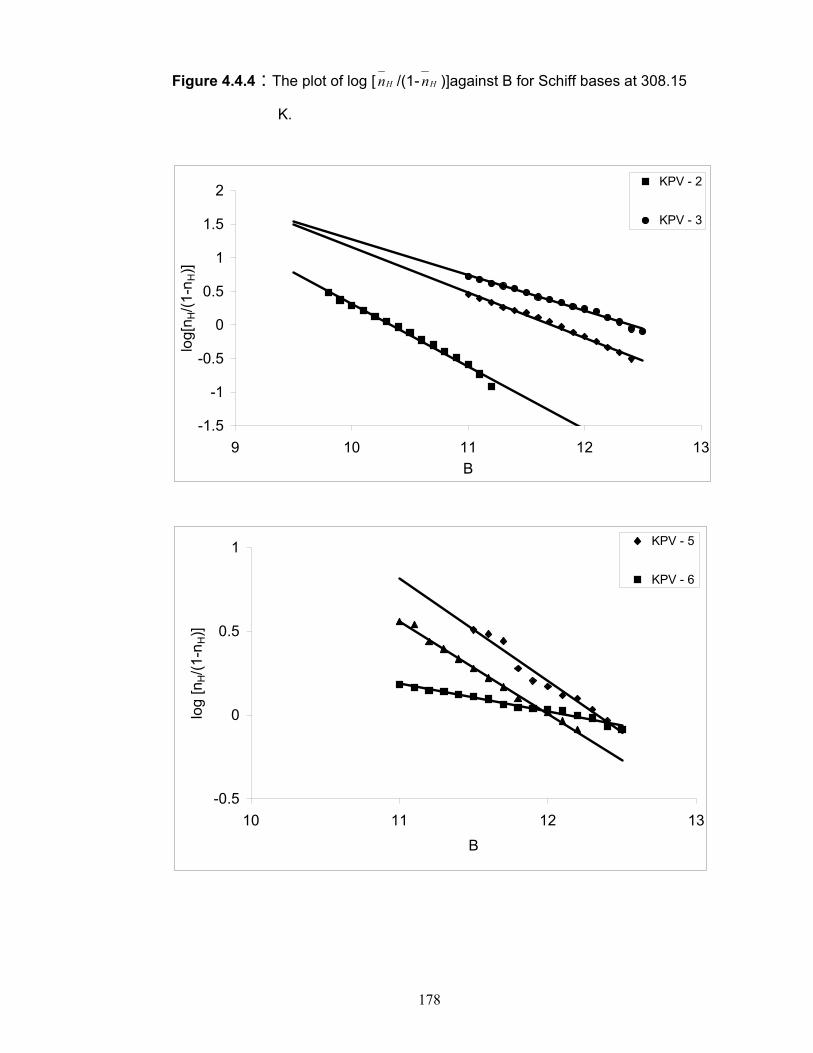
178

Figure 4.4.4 : The plot of log [ Hn /(1- Hn )]against B for Schiff bases at 308.15

K.

-1.5

-1

-0.5

0

0.5

1

1.5

2

9 10 11 12 13B

log[

n H/(1

-nH)]

KPV - 2

KPV - 3

-0.5

0

0.5

1

10 11 12 13

B

log

[nH/(1

-nH)]

KPV - 5

KPV - 6

179

Figure 4.4.5 : The plot of log [ Hn -1/(2- Hn )]against B for KPV-1 at 308.15

K.

-1.5

-1

-0.5

0

0.5

1

1.5

9 10 11 12 13B

log

[nH

-1/(2

-nH)]

180

( )( )1log log

1HH

H

npK B

n

= +

− ………. (4.4.21)

From these log pK1H values, the average value of pK1

H can be

calculated.

For KPV-1 base, the proton-ligand constants were calculated by

solving equation (4.4.1). For all the points below Hn =1, the following equation

was used. ( )( )1log log

1HH

H

npK B

n

= +

− ………. (4.4.22)

where as for all the points above Hn =1, the equation used was:

( )( )2

1log log

2HH

H

npK B

n

− = +

− ………. (4.4.23)

The plot of log ( )( )

1

2

nH

nH

−

−

against B gives a straight line and are

shown in Figure 4.4.5. The values of log pK1H and log pK2

H are given in Table

4.4.1

The dissociation constants of all the Schiff bases were also evaluated

by half-integral method. All these values are given in Table 4.4.1. It is

observed that the values calculated by half-integral are in fairly good

agreement with the observed values.

The comparison of pK1H values shows that acidic character changes in

the order: KPV-2 > KPV-4 > KPV-7 > KPV-6 > KPV-3 ≈ KPV-5. The acidic

character depends on the type of substituent group. In KPV-2, -Cl is at ortho

position whereas in KPV-7, it is at para position. Similarly, KPV-4 and KPV-5

contain –NO2 group at ortho and para positions. Thus, it is observed that

presence of –Cl or –NO2 group at ortho position increases the acidic character

whereas at para position, the acidic character is found to decrease. The

presence of intra molecular hydrogen bonding also plays an important role in

deciding the acidic character of a compound. When intra molecular hydrogen

bonding is weak, acidic character increases. In KPV-2 and KPV-4, due to

ortho substitution, there may be some steric hindrance, which may cause

181

some weakening in intra molecular interactions thereby increasing the acidic

character. In case of KPV-1, due to –OH group at ortho position, acidic

character is increased but not as much as KPV-2 and KPV-4.

182

References :

[1] Kreb and Speakman, J. Chem. Soc., (1945) 593.

[2] R. J. Gillespie and S. Solomons, J. Chem. Soc., (1957) 1796.

[3] Farmer and Warth. J. Chem. Soc., 85 (1904) 1713.

[4] H. M. Dawson, G. V. Hall and A. Key, J. Chem., Soc., (1928) 2844.

[5] S. M. C. Buckenmaier, D. V. McCalley and M. R. Euerby, J. Chromato.

A, 1004 (2003) 71.

[6] C. Foulon, C. Vaccher, S. Yous J. P. Bonte and J. F. Goossens, J.

Chromato. A 1035 (2004) 131.

[7] N. Ikuta and T. Hirokawa, Jpn. Kokai. Tokkyo. Koho. Jp., 77 (2004) 405.

[8] H. Tanaka, K. Aritsuka, T. Tachibana, H. Chuman and P. K.Dasgupta,

Anal. Chim. Acta,499 (2003)199.

[9] H. Tanaka, T. Tachibana, R. Oda and P. K. Dasgupta, Talanta, 64

(2004)1169.

[10] D. Olivier, A. Conpe, L. Tache, M. Rager and J. Maquet, Inorg. Chem.,

46 (2004) 2021.

[11] A. Tejernberg, S. Carno, F. Oliv, K. Benkestock, P. O. Edlund and W. J.

Hallen, Anal. Chem. 76 (2004) 4325.

[12] A. S. Albert and E. P.Serjeant, “Ionization Constants of Acids and

Bases”, Methuen and Co., Ltd.

[13] S. Kratsis, G. Hefter, P. M. May and P. S. Kratsis, Austr. J. Chem., 53

(2000) 363.

[14] O. Redlich and G. C. Hood. Disc. Farady Soc., 24 (1957) 87.

[15] D. H. McDanial, H. C. Brown and O. Haffinger E. A. Brande and F.

Nachod, Academic Press, Inc, N. W. (1955).

[16] E. Prenesti, P. G. Daniele, S. Toso, V. Zelano and S. Berto, Chem.

Spec. Bioav., 16 (2004) 1.

[17] I. D. Tabagua and T. R.Sukhumsk, Gos. Ped. Inst. 15 (1962) 110.

[18] E. S. Shcherbakova and E. N. Goldstein, Usp. Khim., 47 (1978) 2134.

183

[19] M. S. Mayadeo and S. S. Purohit, J. Ind. Chem. Soc., LIX (1982) 955.

[20] R. V. Kinhikar and V. S. Jamode, Asian J. Chem., 6 (1994) 174.

[21] M. Y. Harun and M. H. Turk J. Chem., 22 (1998) 209.

[22] Y. K. Meshram, M. L. Narwade and A. Ali, Acta Cien. Ind., XXlX,(2003)

45.

[23] S. E. Blanco and F. H. Ferretti, Chem. Phys. Lett., 403 (2005) 400.

[24] B. S. Garg, M. Chaudhury and R. Dixit, Ind. Acad. Sci., LIX (1982) 949.

[25] J. Ui Hawang, J. Jae Chung and J. E. Lee, J. Korean Chem. Soc. 30

(1986).

[26] F. R. Trull, S. Boiadjiev, D. A. Lightner, A. F. McDonagh, J. Lipid Res.

38 (1997) 1188.

[27] K. Saraswathi, S. S. Babu and Y. Sunandamma, Asian J. Chem., 12

(2000) 313.

[28] F. J. Millero, D. Pierrot, K. Lee, R. Wanninkof, R. Freely, C. L. Sabine,

R. M. Key and T. Takahashi, Oceano. Res. Pap. 49 (2002) 1705.

[29] E. Grunwald, J. Am. Chem. Soc., 73 (1951) 4934.

[30] M. Czaja, A. Kozak, M. Makowski and L. Chmurzyski , J. Chem.

Thermodyn., 35 (2003 ) 1645.

[31] R. S. Sandhu, Anorg. Struk. Phys. Chemie 108 (1977) 51 .

[32] H. S. Harned and Bridsall, J. Am. Chem. Soc., 65 ,(1943) 54,147.

[33] M. Yasuda, Bull. Chem. Soc., (Japan) 32 ,(1952) 429.

[34] M. L. Dondon and J. Paris, J. Chim. Phys., 58 (1961) 222.

[35] N. Y. Lyakira, T. A. Levshina, B.U. Mamzurin, L. V. Shikova and V. P. Y.

Savel,Tr. Mosk. Khim. Teknol. Inst. 70 ,(1972) 25.

[36] C. C. Panichaiakul and E. M. Woolley, Anal. Chem., 47 ,(1975) 1860.

[37] C. P. Gupta, K. G. Sharma, R. P. Mathur and R. K. Mehta, Acta. Chim.

Acad. Sci., 111 ,(1982) 19.

[38] C. K. Ramaiah and K. Ram, J. Ind. Chem. Soc., 74 (1997) 90.

184

[39] B. R. McRae, B. A. Patterson, M. L. Origlia -Luster, J. Chem.

Thermodyn., 35 (2003)301.

[40] L. Pardeshi and R. A. Bhole, J. Ind. Chem. Soc., LVII (1980) 971.

[41] H. Arora, A. Aggarwal and R. P. Singh, J. Ind. Chem. Soc., LIX (1982)

347.

[42] N. Etxebarria, M. J. Zapatero,J. M. Castresana, L. A. Fernandez, M. A.

Olazabal and J. M. Madariaga, J. Sol. Chem., 20 (1991) 1213.

[43] M. Palanichamy and M. Anbu, Ind. Acad. Sci., 109 (1997) 105 .

[44] K. Rengaraj, B. Sivasankar, M. Anbu and M. Palanichamy, Ind. Acad.

Sci., 104, (1992) 707.

[45] M. A. Robert, D. Ren, R. D’sa and A. H. Abid, Can. J. Chem., 78 (2000)

1178.

[46] A. Boraei and T. I. Ahmed, Synth. Rect. Inorg. Met. Org. Chem., 36

(2002) 981.

[47] F. Javier, M. Prieto and F. J. Millero, Geo. Cosmo. Acta., 66 (2002) 2529.

[48] J. Ghaseni, S. Ahmadi, M. Kubista and A. Forootan, J. Chem. Eng. Data,

48 (2003) 1178.

[49] M. Remko and Claus –Wilhem von der Lieth,Bioorg. Med. Chem.Lett. 12

(2004) 5395.

[50] J. I. Partanen and A. K.Covington, J. Chem. Eng. Data, 49 (2004) 394 .

[51] J. A. Riddick, W. B. Bunger and Sakano, “ Organic solvents-Physical

properties and methods for purification, IV th Edition, Techniques of

Chemistry vol. II, A. Wiley- Intersicence publication- John-Wiley.

[52] J. Bjerrum, “Metal Amine Formation in Aqueous Solution”, P. Hasse and

Sons, Copenhagen (1941).

[53] H. Irving and H. S. Rossoti, J. Chem Soc., (1954) 2094.

[54] C. G. Van Uitert and C. G. Hass, J. Am. Chem. Soc., 75 (1953) 451.

CHAPTER - IV

SECTION - 5

ACOUSTICAL PROPERTIES

185

In this chapter, various acoustical parameters have been evaluated from

experimental data of Ultrasonic velocity, density and viscosity of solutions of

some Schiff bases in dimethylformamide (DMF) and dimethylsulfoxide

(DMSO) at 308.15 K.

Introduction :

The name Ultrasound is given to sound waves having frequencies

higher than those to which the human ear can respond (i.e.> 20 KHz ). It is

also known as silent sound waves.

In recent years, Ultrasonic has become the subject of extensive

research in wide range of application in different fields like chemical

industries, consumer industries, medical field, process industries, food

industry, physics, chemistry and biology etc [1-13]. As it is a non-destructive

technique, it attracts more attention. In medical field, this technique has been

used to detect gall stones, cancerous tissues, and foreign bodies in tissues.

Further ultrasonic studies on hemoglobin, myoglobin and borine serum

albumin have been reported [8-10]. In chemistry, ultrasonic waves are knows to

be useful to chemical reactions and processes. Ultrasound waves have

proven to enhance reaction yields in more convenient reaction conditions[14-17].

Further, it helps to understand the molecular interactions in liquid[18]. liquid

mixtures[19-25] and solutions[26-33]. Various thermodynamic properties can be

also studied by measuring acoustical parameters in liquid mixtures and

solutions.

Literature survey shows that much work has been done in pure

liquids[34-36], liquid mixtures[37-48] and solutions of inorganic salts[49-52], amino

acid[53-56], polymers[57-60 ] etc.

However scanty work has been done for organic compounds [61-65]

specially Schiff bases [66-69].

Thus, in the present chapter, acoustical properties of solutions of some

Schiff bases have been studied in DMF and DMSO at 308.15 K.

186

Experimental :

The solvents dimethyl formamide (DMF) and dimethylsulfoxide

(DMSO), used in the present study are purified by standard methods. The

mole fraction of purity was better than 0.995 for both the solvents.

The solutions of all the Schiff bases were prepared in both the solvents

over the wide range of concentrations. The densities, viscosities and

ultrasonic velocities of pure solvents and solutions of different concentration

were measured at 308.15 K by using pyknometer, an Ubbelohde suspended

level viscometer and ultrasonic interferometer operating at 2 MHz with the

uncertainties of 0.0001 g/cm3, + 0.06 % and 0.01% respectively.

Density measurement :

The weight of distilled water, pure solvents and solutions of Schiff

bases were measured by using pyknometer. The densities were evaluated by

using following equation :

ρ (g/cc)=[(wt. of solvent or solution)/(wt. of water)] x [density of water].. (4.5.1)

Viscosity measurement :

To determine viscosity of solution the determine the Ubbeholde

viscometer [70] was used, which obeys Stoke’s low[71]. The measured quantity

of the distilled water / solvent / solution was placed in the viscometer, which

was suspended in a thermostat at 308.15 + 0.1 K. The digital stopwatch with

an accuracy of + 0.01 sec was used to determine flow time of solutions. Using

the flow times (t) and known viscosity of standard water sample the viscosity

of solvent and solution were determined according to equation:

η1 / η2 = t1ρ1 / t2ρ2 ……….(4.5.2)

Sound velocity measurement :

Ultrasonic interferometer (Model No. F-81), Mittal Enterprise, New

Delhi, working at frequency of 2 MHz was used to determine sound velocity.

187

The solvent / solution was filled in the measuring cell with quartz crystal

and then micrometer was fixed. The circulation of water from the thermostat

maintained at 308.15 K was started and test solvent /solution in the cell is

allowed to thermally equilibrate. The micrometer was rotated very slowly so as

to obtain a maximum or minimum of anode current (n). A number of maximum

readings of anode current were counted.

The total distance (d) traveled by the micrometer for n=10, was read.

The wavelength (λ) was determined according to the equation (4.5.3).

λ = 2d / n ………. (4.5.3)

The sound velocity (U) of solvent and solutions were calculated from the

wavelength and frequency (F) according to equation (4.5.4).

U = λ F ………. (4.5.4)

188


The density (ρ), viscosity (η) and sound velocity (U) of pure solvents

and different Schiff bases solutions in dimethylformamide (DMF) and

dimethylsulfoxide (DMSO) were calculated at 308.15 K and are reported in

Table 4.5.1.

From these measurements, various acoustical parameters like specific

acoustical impendence (Z), isentropic compressibility (κs), intermolecular free

length (Lf), Rao’s molar sound function (Rm), molar compressibility (W),

Vander Waals constant (b), relaxation strength (r), internal pressure (π),

solvation number (Sn) etc. were evaluated using the following equations:

1. Specific acoustical impedance :

Specific acoustical impedance (Z) can be calculated as:

Z = Uρ ………. (4.5.5)

2. Isentropic compressibility :

Isentropic compressibility (κs) can be evaluated according to the

following the equation [72].

κs = 1/U2ρ ………. (4.5.6)

3. Intermolecular free path length :

Jacobson [73] proposed an equation for calculating the inter molecular

free path length (Lf), which is given below:

Lf = KJ κs 1/2 ………. (4.5.7)

where KJ is Jacobson constant (=6.0816 x 104)

4. Rao’s molar sound function :

Rao’s molar sound function (Rm) can be evaluated by an equation

given by Bagchi et al [74].

Rm = (M/ρ) U1/3 ………. (4.5.8)

189

Table 4.5.1: The density (ρ), ultrasonic velocity (U) and viscosity (η) of Schiff

bases in DMF and DMSO at 308.15 K.

Conc. (M)

Density ρ

(gm.cm-3)

VelocityU . 10-5 (cm.s-1)

Viscosityη . 103

(poise)

Density ρ

(gm.cm-3)

Velocity U . 10-5 (cm.s-1)

Viscosityη . 103 (poise)

DMF DMSO

KPV - 1 KPV - 1

0.00 0.9356 1.4380 0.6780 1.0853 1.4648 0.9425 0.01 0.9366 1.4468 0.6940 1.0879 1.5156 1.6036 0.02 0.9378 1.4492 0.7013 1.0886 1.4940 1.6696 0.04 0.9386 1.4536 0.7215 1.0889 1.4884 1.6945 0.06 0.9396 1.4588 0.7431 1.0892 1.4874 1.7079 0.08 0.9405 1.4616 0.7490 1.0896 1.4820 1.7349 0.10 0.9413 1.4648 0.7674 1.0899 1.4816 1.7510

KPV - 2 KPV - 2

0.01 0.9382 1.4476 0.6857 1.0887 1.4684 1.3822 0.02 0.9388 1.4424 0.6893 1.0890 1.4656 1.4325 0.04 0.9401 1.4400 0.7211 1.0893 1.4632 1.4770 0.06 0.9411 1.4388 0.7277 1.0899 1.4608 1.5167 0.08 0.9413 1.4364 0.7388 1.0901 1.4596 1.5682 0.10 0.9416 1.4336 0.7539 1.0912 1.4584 1.6263

KPV - 3 KPV - 3

0.01 0.9380 1.4432 0.6828 1.0907 1.4800 1.6506 0.02 0.9404 1.4492 0.7108 1.0909 1.4780 1.6884 0.04 0.9429 1.4556 0.7401 1.0922 1.4744 1.7123 0.06 0.9444 1.4580 0.7605 1.0926 1.4720 1.7331 0.08 0.9452 1.4624 0.7825 1.0960 1.4704 1.7605 0.10 0.9472 1.4680 0.8143 1.0971 1.4688 1.8940

KPV - 4 KPV - 4

0.01 0.9408 1.4780 0.7170 1.0926 1.4904 1.7389 0.02 0.9414 1.4644 0.7236 1.0930 1.4872 1.7551 0.04 0.9433 1.4600 0.7360 1.0937 1.4848 1.7844 0.06 0.9441 1.4592 0.7499 1.0945 1.4820 1.8061 0.08 0.9446 1.4576 0.7556 1.0963 1.4744 1.8760 0.10 0.9459 1.4524 0.7671 1.0976 1.4708 1.9278

190

Continue…. (Table: 4.5.1)

Conc. (M)

Density ρ

(gm.cm-3)

VelocityU . 10-5

(cm.s-1)


Density ρ

(gm.cm-3)

Velocity U . 10-5 (cm.s-1)


DMF DMSO

KPV - 5 KPV - 5

0.01 0.9382 1.4344 0.6795 1.0925 1.4384 1.7503 0.02 0.9403 1.4372 0.6949 1.0937 1.4516 1.8064 0.04 0.9412 1.4404 0.6970 1.0942 1.4600 1.8429 0.06 0.9422 1.4472 0.7094 1.0944 1.4716 1.8901 0.08 0.9444 1.4496 0.7367 1.0953 1.4784 2.0244 0.10 0.9482 1.4544 0.7634 1.0953 1.4840 2.0701

KPV - 6 KPV - 6

0.01 0.9412 1.4480 0.7224 1.0940 1.4692 2.0726 0.02 0.9414 1.4500 0.7315 1.0946 1.4616 2.0724 0.04 0.9430 1.4528 0.7478 1.0949 1.4516 2.0601 0.06 0.9438 1.4544 0.7664 1.0956 1.4460 1.9979 0.08 0.9453 1.4556 0.7908 1.0969 1.4364 1.9229 0.10 0.9459 1.4592 0.8103 1.0971 1.4284 1.8789

KPV - 7 KPV - 7

0.01 0.9373 1.4712 0.7622 1.0918 1.5040 1.6592 0.02 0.9397 1.4700 0.7724 1.0922 1.4952 1.7913 0.04 0.9431 1.4664 0.7829 1.0924 1.4912 1.8488 0.06 0.9441 1.4640 0.7954 1.0925 1.4808 1.9757 0.08 0.9479 1.4624 0.8724 1.0927 1.4692 2.0243 0.10 0.9498 1.4568 0.9667 1.0929 1.4484 2.2283

KPV - 8 KPV - 8

0.01 0.9439 1.4788 0.9987 1.0928 1.5148 1.8429 0.02 0.9446 1.4728 1.0339 1.0935 1.5112 1.9183 0.04 0.9457 1.4688 1.1051 1.0954 1.5008 1.9434 0.06 0.9476 1.4640 1.1893 1.0957 1.4912 2.0736 0.08 0.9480 1.4628 1.2796 1.0962 1.4828 2.1239 0.10 0.9487 1.4540 1.3809 1.0965 1.4748 2.7090

191

The apparent molecular weight (M) of the solution can be calculated

according to equation (4.5.9) :

M = M1W1 + M2W2 ………. (4.5.9)

where W1 and W2 are weight fractions of solvent and solute respectively. M1 and

M2 are the molecular weights of the solvent and compounds respectively.

5. Molar compressibility :

Molar compressibility (W) can be calculated by the following equation[75].

W = (M/ρ) κs -1/7 ………. (4.5.10)

6. Van der Waals Constant :

Van der Waals constant (b) can be calculated as follows [76].

b = M/ρ 1- (RT/MU2) √ [1 +(MU2/ 3RT) – 1] ………. (4.5.11)

where R is the gas constant (=8.3143 JK-1 mol-1) and T is the absolute

temperature.

7. Relaxation Strength :

The relaxation strength (r) can be calculated as follows [77].

r = 1- [U/U∞] 2 ………. (4.5.12)

where U∞ = 1.6 x 105 cm/s.

8. Internal Pressure :

Suryanarayana and Kuppuswamy[78] gave the following equation for

evaluating internal pressure:

π = bRT [Kη/U] 1/2 ρ2/3/M7/6 ………. (4.5.13)

192

where b is the packing factor (= 2). K is a constant (=4.28 X 109). The internal

pressure (π) depends on temperature, density, ultrasonic velocity and specific

heat at constant pressure.

9. Solvation Number :

The solvation number (Sn) can be evaluated according to Passynsky[79]

method.

Sn = M2 / M1 [1-κs /κs 1] [(100-X)/X] ……… (4.5.14)

where X is the number of grams of solute in 100 g. of the solution and M1 and M2

are the molecular weights of solvent and solute respectively. κs1 and κs are the

isentropic compressibility of solvent and solution, respectively.

These acoustical parameters are useful for the understanding of molecular

interactions in a solution. Some of these parameters are given in Tables 4.5.2

and 4.5.3 for Schiff bases in DMF and DMSO at 308.15 K.

Further, some of these parameters were also correlated with

concentration. The correlation coefficients along with correlation equation for

these parameters are given in Tables 4.5.4 and 4.5.5 for all the Schiff bases in

both the solvents.

Fig. 4.5.1 and Fig. 4.5.2 shows the variation of ultrasonic velocity with

concentration for Schiff bases solutions in DMF and DMSO. It is observed from

these figures that in DMF, ultrasonic velocity (U) increases with concentration for

KPV-1, KPV-3, KPV- 5 and KPV- 6 and decreases for KPV-2, KPV-4, KPV-7 and

KPV-8 where as in DMSO, velocity is found to decrease with increase in

concentration for all Schiff bases except KPV- 5.

The ultrasonic velocity depends on intermolecular free path length (Lf).

The ultrasonic velocity U increases with decrease in intermolecular free path

length (Lf) and vice versa. The variation of intermolecular free length (Lf) against

concentration is shown in Fig. 4.5.3 and 4.5.4 for Schiff base solutions in both the

solvents. It is obvious that in DMF, Lf decreases for KPV-1, KPV-3, KPV-5 and

193

KPV-6 where as it increases for KPV-2, KPV-4, KPV-7 and KPV-8. This is

reverse of Fig. 4.5.1 and 4.5.2 as expected. Similarly, Lf is found to increase with

concentration in DMSO for all Schiff bases except KPV-5. The increase in

ultrasonic velocity and decrease in Lf indicates close association between solute

and solvent molecules. Where as decrease in velocity and increase in Lf suggest

predominance of solute –solute interactions.

The predominance of a particular interaction in a particular solution can

also be decided by isentropic compressibility, which is shown in Fig. 4.5.5 and

4.5.6 for all the bases in DMF and DMSO respectively. It is observed that in DMF

solution, isentropic compressibility decreases with increase in concentration for

KPV-1, KPV-3, KPV-5 and KPV-6. However, it decreases only for KPV-5 in

DMSO. It is observed from Table 4.5.2 that in DMF solutions, relaxation strength

(r) also decreases with increase in concentration for KPV-1, KPV-3, KPV-5 and

KPV-6 where as it increases for KPV-2, KPV-4 KPV-7 and KPV-8. However,

acoustic impedance (Z) shows reverse nature. In DMSO solutions (Table 4.5.3),

only for KPV-5, Z increases and r decreases with concentration. For all other

Schiff bases, Z decreased and relaxation strength (r) increased with

concentration. The increase in Z and decrease in κs and r again proves the

existence of solute-solvent[80] interactions in KPV-1, KPV-3, KPV-5 AND KPV-6

(in DMF) and KPV-5 (in DMSO). The increase in isentropic compressibility (κs)

and relaxation strength (r) in other Schiff bases, KPV-2, KPV-4, KPV-7, KPV-8 in

DMF and all other bases except KPV-5 in DMSO suggests the predominance of

solute-solute interactions.

It is obvious from Tables 4.5.4 and 4.5.5 that Rao’s molar function (Rm),

molar compressibility (W) and Vander Waal’s constant (b) vary linearly with

concentration for all the Schiff bases in both the solvents. This suggests the

absence of complex formation in these solutions.

The internal pressure (π) is the resultant of the forces of attraction and

repulsion between the molecules in a liquid. It is observed from the Tables 4.5.2

that in DMF, except for KPV-1 and KPV-2, π values are first increasing and then

194

decreasing. For KPV-3, KPV-6, KPV-7 and KPV-8, it increased continuously. For

KPV-4, it decreases continuously whereas for KPV-5, π values first decreased

and then increased. In DMSO, except KPV-6, for other bases, internal pressure

values are found to increase. The increase in π values indicate the solute-solvent

interactions. Thus, it is observed that in these systems, both solute-solute and

solute-solvent interactions exist although some acoustical properties suggest the

predominance of one type of interaction.This is again confirmed by solvation

number (Sn).

The solvation number (Sn) is a measure of structure forming or structure

breaking tendency of solute in a solution. The increase in Sn values indicates

the structure-forming tendency of solute or vice versa. Fig.4.5.7 and 4.5.8

shows the variation of Sn with concentration in both DMF and DMSO

respectively. It is observed that in both DMF and DMSO solutions, except KPV-

6, other bases show structure-forming tendency. The Sn decreases with

concentration in both DMF and DMSO for KPV-6, suggesting thereby structure-

breaking tendency of this Schiff base.

Overall, both solute-solute and solute-solvent interactions exist in these

solutions of Schiff bases in both the solutions.

195

Table 4.5.2: Variation of acoustical parameters with concentration of Schiff bases in DMF at 308.15 K.

Conc. (M)

Specific Impedance

Z.10 -5 (gm.cm-2)

RelaxationStrength

r

Rao’s molar Sound Function

Rm.10-3 (cm-8/3.sec-1/3)

Molar Compressibility

W.10-3 (cm-1.dyn-1)

Van der Waal’sconstant

b (cm3.mol-1)

Internal Pressure

π

KPV - 1 0.00 1.3454 0.1922 4.0934 2.3033 73.4366 465.60060.01 1.3551 0.1823 4.1152 2.3152 73.7088 467.58560.02 1.3591 0.1796 4.1300 2.3238 73.9475 467.67800.04 1.3643 0.1746 4.1663 2.3442 74.5490 469.21170.06 1.3707 0.1687 4.2024 2.3644 75.1341 470.96710.08 1.3746 0.1655 4.2366 2.3838 75.7191 468.05150.10 1.3788 0.1619 4.2715 2.4035 76.3113 468.9551

KPV - 2 0.01 1.3581 0.1814 4.1130 2.3145 73.6596 464.64990.02 1.3541 0.1873 4.1273 2.3231 74.0008 464.02330.04 1.3537 0.1900 4.1628 2.3438 74.6924 469.64900.06 1.3541 0.1913 4.2006 2.3655 75.4079 466.62230.08 1.3521 0.1940 4.2408 2.3884 76.1846 465.03290.10 1.3499 0.1972 4.2800 2.4108 76.9509 464.7559

KPV - 3 0.01 1.3537 0.1864 4.1087 2.3123 73.6456 464.43700.02 1.3628 0.1796 4.1246 2.3217 73.8536 470.91550.04 1.3725 0.1724 4.1611 2.3426 74.4316 474.74010.06 1.3769 0.1696 4.1998 2.3637 75.1073 475.84610.08 1.3823 0.1646 4.2399 2.3873 75.7766 476.74900.10 1.3905 0.1582 4.2771 2.4085 76.3778 480.7038

KPV - 4 0.01 1.3905 0.1467 4.1326 2.3241 73.5763 470.75620.02 1.3786 0.1623 4.1416 2.3305 73.9414 472.06410.04 1.3772 0.1673 4.1775 2.3517 74.6676 470.98330.06 1.3776 0.1683 4.2215 2.3768 75.4873 469.48480.08 1.3768 0.1701 4.2660 2.4021 76.3276 465.47940.10 1.3738 0.1760 4.3029 2.4238 77.0879 464.1697

196

Continue…. DMF

Conc. (M)

Specific Impedance

Z.10 -5 (gm.cm-2)

RelaxationStrength

r


Rm.10-3 (cm-8/3.sec-1/3)


W.10-3 (cm-1.dyn-1)


b (cm3.mol-1)

Internal Pressure

π

KPV - 5 0.01 1.3458 0.1963 4.1030 2.3099 73.6723 464.34990.02 1.3514 0.1931 4.1207 2.3204 73.9604 466.59390.04 1.3557 0.1895 4.1682 2.3472 74.7883 460.74750.06 1.3636 0.1819 4.2187 2.3755 75.6143 457.86190.08 1.3690 0.1792 4.2591 2.3988 76.3240 460.81260.10 1.3791 0.1737 4.2939 2.4194 76.8954 463.5474

KPV - 6 0.01 1.3629 0.1810 4.0911 2.3032 73.2572 479.13330.02 1.3650 0.1787 4.1047 2.3108 73.4789 480.14570.04 1.3700 0.1755 4.1256 2.3229 73.8234 482.06840.06 1.3727 0.1737 4.1488 2.3361 74.2263 484.60110.08 1.3760 0.1724 4.1684 2.3476 74.5703 489.11410.10 1.3803 0.1683 4.1943 2.3621 74.9912 491.2657

KPV - 7 0.01 1.3790 0.1545 4.1392 2.3271 73.7896 485.62000.02 1.3814 0.1559 4.1494 2.3338 73.9983 486.86950.04 1.3830 0.1600 4.1745 2.3494 74.5164 486.01200.06 1.3822 0.1628 4.2112 2.3706 75.2249 484.71480.08 1.3862 0.1646 4.2353 2.3857 75.6985 503.32860.10 1.3837 0.1710 4.2639 2.4029 76.3123 525.3829

KPV - 8 0.01 1.3958 0.1458 4.1200 2.3181 73.3397 556.64140.02 1.3912 0.1527 4.1358 2.3277 73.7178 563.89090.04 1.3890 0.1573 4.1760 2.3510 74.5139 576.26450.06 1.3873 0.1628 4.2115 2.3720 75.2381 591.56450.08 1.3867 0.1641 4.2571 2.3979 76.0908 605.87500.10 1.3794 0.1742 4.2936 2.4195 76.8969 623.3630

197

Table 4.5.3: Variation of acoustical parameters with concentration of Schiff bases in DMSO at 308.15 K.

Conc. (M)

Specific Impedance

Z.10 -5 (gm.cm-2)

RelaxationStrength

r


Rm.10-3 (cm-8/3.sec-1/3)


W.10-3 (cm-1.dyn-1)


b (cm3.mol-1)

Internal Pressure

π

KPV - 1 0.00 1.5863 0.1655 3.7921 2.1778 67.8284 556.23250.01 1.6253 0.1281 3.8237 2.1944 68.0190 715.96840.02 1.6220 0.1328 3.8306 2.1988 68.1625 728.98040.04 1.6203 0.1346 3.8550 2.2130 68.6036 723.68750.06 1.6196 0.1358 3.8790 2.2269 69.0510 723.78750.08 1.6142 0.1421 3.8989 2.2388 69.4813 722.50180.10 1.6148 0.1425 3.9216 2.2520 69.9290 723.1596

KPV - 2 0.01 1.5986 0.1577 3.8019 2.1839 67.9215 670.19510.02 1.5960 0.1609 3.8143 2.1913 68.1860 679.73960.04 1.5939 0.1637 3.8427 2.2079 68.7405 684.28520.06 1.5921 0.1664 3.8700 2.2239 69.2748 687.65540.08 1.5911 0.1678 3.8998 2.2412 69.8371 693.02900.10 1.5914 0.1692 3.9261 2.2567 70.3385 699.9337

KPV - 3 0.01 1.6142 0.1444 3.8041 2.1849 67.8085 730.55970.02 1.6124 0.1467 3.8168 2.1924 68.0665 736.05700.04 1.6103 0.1508 3.8391 2.2059 68.5255 735.99630.06 1.6083 0.1536 3.8656 2.2214 69.0430 734.53190.08 1.6116 0.1554 3.8817 2.2317 69.3650 735.68370.10 1.6114 0.1573 3.9060 2.2461 69.8336 757.2291

KPV - 4 0.01 1.6284 0.1323 3.8090 2.1875 67.7602 747.50120.02 1.6255 0.1360 3.8225 2.1956 68.0497 747.91920.04 1.6239 0.1388 3.8531 2.2136 68.6423 747.05000.06 1.6220 0.1421 3.8830 2.2312 69.2260 744.72250.08 1.6164 0.1508 3.9047 2.2448 69.7311 753.86740.10 1.6144 0.1550 3.9316 2.2609 70.2748 757.8773

198

Continue…. DMSO Conc.

(M) Specific

Impedance Z.10 -5

(gm.cm-2)

RelaxationStrength

r


Rm.10-3 (cm-8/3.sec-1/3)


W.10-3 (cm-1.dyn-1)


b (cm3.mol-1)

Internal Pressure

π

KPV - 5 0.01 1.5715 0.1918 3.7645 2.1656 67.6502 763.34150.02 1.5876 0.1769 3.7893 2.1793 67.9263 768.36870.04 1.5975 0.1673 3.8298 2.2021 68.5549 765.84960.06 1.6105 0.1541 3.8742 2.2269 69.2092 764.48480.08 1.6193 0.1462 3.9120 2.2483 69.8061 781.55970.10 1.6254 0.1397 3.9520 2.2709 70.4590 780.6788

KPV - 6 0.01 1.6073 0.1568 4.0911 2.1713 67.4706 824.83030.02 1.5999 0.1655 4.1047 2.1722 67.5811 824.93400.04 1.5894 0.1769 4.1256 2.1778 67.8687 820.90420.06 1.5842 0.1832 4.1488 2.1844 68.1404 805.90350.08 1.5756 0.1940 4.1684 2.1882 68.3638 789.56840.10 1.5671 0.2030 4.1943 2.1946 68.6598 778.5227

KPV - 7 0.01 1.6421 0.1164 4.1392 2.1935 67.8057 726.92840.02 1.6331 0.1267 4.1494 2.1983 68.0498 754.05160.04 1.6290 0.1314 4.1745 2.2144 68.6044 759.84800.06 1.6178 0.1434 4.2112 2.2279 69.1508 780.81410.08 1.6054 0.1568 4.2353 2.2406 69.6873 786.12000.10 1.5830 0.1805 4.2639 2.2491 70.2014 823.0397

KPV - 8 0.01 1.6554 0.1037 4.1200 2.1975 67.8036 763.36850.02 1.6525 0.1079 4.1358 2.2050 68.0769 775.84290.04 1.6440 0.1202 4.1760 2.2178 68.5823 776.09590.06 1.6339 0.1314 4.2115 2.2336 69.1887 795.83620.08 1.6254 0.1411 4.2571 2.2494 69.7836 799.45050.10 1.6171 0.1504 4.2936 2.2657 70.3913 896.0518

199

Fig. 4.5.1 : Variation of ultrasonic velocity (U) against concentration for Schiff

bases in DMF at 308.15 K.

1.42

1.46

1.5

0 0.04 0.08 0.12

Concentration (M)

Vel

ocity

.10-5

(cm

/sec

)

KPV - 5KPV - 6KPV - 7KPV - 8

200

Fig. 4.5.2 : Variation of ultrasonic velocity (U) against concentration for

Schiff bases in DMSO at 308.15 K.

201

Table 4.5.4 : The correlation coefficient (γ) and correlation equations

between some acoustical parameters and concentrations (C)

of Schiff bases in DMF solutions at 308.15 K.

Parameters γ Correlation equation

KPV-1

U (cm.sec-1) 0.9946 U – 20285 C = 144532

W (cm-1.dyn-1) 0.9998 W – 988.26 C = 2304.8

b (cm3.mol-1) 0.9998 b - 29.17 C = 73.388

Rm (cm-8/3.sec-1/3) 0.9999 Rm -1752.9 C = 4096.5

η (poise) 0.9911 η + 8.20E-3 C = 6.90E-3

r 0.9947 r + 0.2307 C = 0.184

KPV-2

U (cm .sec-1) 0.9582 U + 13381 C = 141671

W (cm-1.dyn-1) 0.9995 W – 1078.4 C = 2302.0

b (cm3.mol-1) 0.9993 b – 36.549 C = 73.261

Rm (cm-8/3.sec-1/3) 0.9992 Rm -1872.2 C = 4119.8

η (poise) 0.9772 η - 7.60E-3 C = 6.80E-3

r 0.9578 r - 0.1505 C = 0.1824

KPV-3

U (cm.sec-1) 0.9827 U – 25173 C = 144306

W (cm-1.dyn-1) 0.9996 W – 1078.2 C = 2300.5

b (cm3.mol-1) 0.9989 b - 31.046 C = 73.261

Rm (cm-8/3.sec-1/3) 0.9997 Rm – 1890.7 C = 4087.5

η (poise) 0.9918 η - 1.30E-2 C = 6.80E-3

r 0.9830 r + 0.2863 C = 0.1866

KPV-4

U (cm.sec-1) 0.8698 U + 21885 C = 147324

W (cm-1.dyn-1) 0.9973 Rm -1963.5 C = 4105.6

b (cm3.mol-1) 0.8698 U + 21885 C = 147324

Rm (cm-8/3.sec-1/3) 0.9982 W – 1141.8 C = 2309.2

η (poise) 0.9943 η - 5.50E-3 C = 7.10E-3

r 0.8687 r - 0.2503 C = 0.1522

202


KPV-5

U (cm. sec-1) 0.9942 U – 22115 C = 143244

W (cm-1.dyn-1) 0.9987 W – 1248.4 C = 2297.4

b (cm3.mol-1) 0.9982 b - 36.979 C = 73.299

Rm (cm-8/3. sec-1/3) 0.9982 Rm -2185.4 C = 4081

η (poise) 0.9665 η - 8.60E-3 C = 6.70E-3

r 0.9959 r + 8.87E-2 C = 4.385E-1

KPV-6

U (cm.sec-1) 0.9868 U - 11353 C = 144747

W (cm-1.dyn-1) 0.9995 W – 642.48 C = 2297.2

b (cm3.mol-1) 0.9996 b – 18.981 C = 73.077

Rm (cm-8/3.sec-1/3) 0.9993 Rm -1121.6 C = 4080.9

η (poise) 0.9979 η - 9.8E-3 C = 7.10E-3

r 0.9867 r + 0.1289 C = 0.1816

KPV-7

U (cm. sec-1) 0.9865 U + 14981 C = 147287

W (cm-1.dyn-1) 0.9988 W – 856.81 C = 2317.3

b (cm3. mol-1) 0.9985 b - 28.42 C = 73.455

Rm (cm-8/3.sec-1/3) 0.9982 Rm – 1416.3 C = 4122.4

η (poise) 0.9692 η - 2.09E-2 C = 7.20E-3

r 0.9866 r – 0.1714 C = 0.1526

KPV-8

U (cm.sec-1) 0.9767 U + 24142C = 147934

W (cm-1.dyn-1) 0.9996 W – 1133.3 C = 2305.5

b (cm3.mol-1) 0.9998 b - 39.457 C = 72.938

Rm (cm-8/3.sec-1/3) 0.9994 Rm -1953.5 C = 4098.1

η (poise) 0.9977 η - 4.22E-2 C = 9.50E-3

r 0.9767 r - 0.2766 C = 0.1452

203

Fig. 4.5.3 : Variation of Inter molecular free path length (Lf) against

concentration for Schiff bases in DMF at 308.15 K.

0.42

0.43

0.44

0 0.04 0.08 0.12

Concentration (M)

L f (

A0 )


204

Fig. 4.5.4 : Variation of Inter molecular free path length (Lf) against

concentration for Schiff bases in DMSO at 308.15 K.

0.38

0.39

0.40

0 0.04 0.08 0.12

Concentration (M)

L f (

A0 )


0.38

0.39

0.40

0.41

0 0.04 0.08 0.12

Concentration (M)

L f (

A0 )


205

Table 4.5.5 : The correlation coefficient (γ) and correlation equations

between some acoustical parameters and concentrations (C)

of Schiff bases in DMSO solutions at 308.15 K.

Parameters γ Correlation equation KPV-1

U (cm.sec-1) 0.9636 U + 13189 C = 149405

W (cm-1.dyn-1) 0.9994 W - 650.53 C = 2187.00

b (cm3.mol-1) 0.9996 b - 22.016 C = 67.738

Rm (cm-8/3.sec-1/3) 0.9992 Rm – 1107.6 C = 3810.9

η (poise) 0.9209 η - 1.19E-2 C = 1.62E-2

r 0.9636 r - 0.1532 C = 0.1281

KPV-2

U (cm.sec-1) 0.9714 U + 10630 C = 146816

W (cm-1.dyn-1) 0.9999 W – 815.41 C = 2175.4

b (cm3.mol-1) 0.9999 b - 27.032 C = 67.653

Rm (cm-8/3.sec-1/3) 0.9998 Rm – 1392.9 C = 3787.2

η (poise) 0.9950 η - 2.55E-2 C = 1.37E-2

r 0.9711 r - 0.1215 C = 0.158

KPV-3

U (cm. sec-1) 0.9825 U + 12351 C = 148031

W (cm-1.dyn-1) 0.9989 W – 675.06 C = 2178.9

b (cm3.mol-1) 0.9983 b - 22.312 C = 67.621

Rm (cm-8/3.sec-1/3) 0.9984 Rm – 1121.9 C = 3794.3

η (poise) 0.9275 η - 2.24E-2 C = 1.62E-2

r 0.9823 r – 0.1422 C = 0.144

KPV-4

U (cm .sec-1) 0.9857 U + 21436 C = 149268

W (cm-1.dyn-1) 0.9990 W – 816.77 C = 2180.1

b (cm3.mol-1) 0.9996 b - 27.968 C = 67.502

Rm (cm-8/3.sec-1/3) 0.9986 Rm – 1366.7 C = 3796.7

η (poise) 0.9808 η - 2.06E-2 C = 1.71E-2

r 0.9858 r – 0.2479 C = 0.1297

206


KPV-5

U (cm.sec-1) 0.9776 U -48395 C = 143900

W (cm-1.dyn-1) 0.9996 W – 1164.8 C = 2155.3

b (cm3.mol-1) 0.9999 b - 31.321 C = 67.316

Rm (cm-8/3.sec-1/3) 0.9995 Rm – 2072.4 C = 3746.5

η (poise) 0.9828 η - 3.54E-2 C = 1.71E-2

r 0.9786 r + 0.5531 C = 0.1913

KPV-6

U (cm.sec-1) 0.9946 U + 43540 C = 147136

W (cm-1.dyn-1) 0.9964 W – 264.99 C = 2167.7

b (cm3.mol-1) 0.9994 b - 13.88 C = 67.333

Rm (cm-8/3.sec-1/3) 0.9932 Rm – 388.76 C = 3771.7

η (poise) 0.9682 η + 2.31E-2 C = 2.12E-2

r 0.9944 r – 0.4927 C = 0.1545

KPV-7

U (cm.sec-1) 0.9772 U + 56526 C = 151067

W (cm-1.dyn-1) 0.9962 W – 643.516 C = 2187.4

b (cm3.mol-1) 0.9999 b - 26.838 C = 67.53

Rm (cm-8/3.sec-1/3) 0.9941 Rm – 1044.2 C = 3811.6

η (poise) 0.9807 η - 5.60E-2 C = 1.63E-2

r 0.9781 r – 0.6524 C = 0.1088

KPV-8

U (cm.sec-1) 0.9989 U + 45359 C = 1511937

W (cm-1.dyn-1) 0.9991 W – 755.45 C = 2189.2

b (cm3.mol-1) 0.9994 b - 28.763 C = 67.485

Rm (cm-8/3.sec-1/3) 0.9987 Rm – 1238.6 C = 3815.2

η (poise) 0.8773 η - 7.92E-2 C = 1.69E-2

r 0.9988 r – 0.5298 C = 0.0984

207

Fig. 4.5.5 : Variation of isentropic compressibility (κs) against

concentration for Schiff bases in DMF at 308.15 K.

4.8

5.0

5.2

0 0.04 0.08 0.12

Concentration (M)

ise.

com

p.10

11 (c

m2 /d

yn)


208

Fig. 4.5.6 : Variation of isentropic compressibility (κs) against

concentration for Schiff bases in DMSO at 308.15 K.

3.9

4.2

4.5

0 0.04 0.08 0.12

Concentration (M)

ise.

com

p.10

11 (c

m2 /d

yn)


4.1

4.2

4.3

4.4

0 0.04 0.08 0.12

Concentration (M)

ise.

com

p.10

11 (c

m2 /d

yn)


209

Fig. 4.5.7 : Variation of Solvation number (Sn) against concentration

for Schiff bases in DMF at 308.15 K.

0

10

20

0.01 0.02 0.04 0.06 0.08 0.1

Concentration (M)

S n


0

5

10

0.01 0.02 0.04 0.06 0.08 0.1

Concentration (M)

Sn


210

Fig. 4.5.8 : Variation of Solvation number (Sn) against concentration

for Schiff bases in DMSO at 308.15 K.

0

40

80

0.01 0.02 0.04 0.06 0.08 0.1

Concentration (M)

S nKPV -1KPV - 2KPV - 3KPV - 4

-10

0

10

0.01 0.02 0.04 0.06 0.08 0.1

Concentration (M)

Sn


211

References:

[1] R. A. Pathrick, J. Macromol. Chem., cg. (1973) 91.

[2] W. Well and R. A. Pethrick, Polumer, 23 (1982) 369.

[3] M. Woldan, J. Phy. Chem., 269 (1988) 628.

[4] G. L. Gooberman, ”Ultrasonics, Theory and Application”. English

Universities Press. Ltd., London EC4 (1968).

[5] M. P. Kapoor, J. Pure Appl. Ultrason, 19 (1997) 104.

[6] W. P. Mason, “Sonics and Ultrasonics, Early history and applications”.,

IEEE Trans Son. Ultrasoni SU-23 (1976) 224.

[7] C. F. Schueler, H. Lee and G. Wade, “Fundamentals of Digital

Ultrasonic Imaging”. IEEE Trans. Sonics and Ultrasonics, SU-31 (1984)

195.

[8] C. Tanford, “In solution of natural polymers”., An International

Symposium held at Edinburgh U.K. published by the Chemical Society,

London. (1968).

[9] K. Kawahara, A. G. Krishner and C. Tanford, Biochemistry, 4 (1965)

1203.

[10] W. D. O. Brien and F. Dunn, J. Acoust. Soc. Am., 50 (1971) 1213.

[11] K. Dhanaraju, R. Balakrishnan, S. Mayilavelan and S. Ramadasse, J.

Pure Appl. Ultrason., 21 (1999) 50.

[12] K. Kumar and R. Prakash, J. Pure appl. Ultrason, 22 (2000) 70.

[13] P. Kumar, H. K. Sharma, P. S. Panesar and G. S. Josan, Proc. Int.

Conf. Ex. Ultra., New Delhi (1999) 111.

[14] T.J.Mason, J.P.Lorimer, “Sonochemistry: Theory, Application and use

of Ultrasound in Chemistry”, Ellis Horwood, Chichester (1988).

[15] C.Enihorn, J, E.Einhorn and J.L.Luche, Synthesis, (1989) 787.

[16] S.K.Mainty, A.K.Chattopadhya and S.C.Lahiri, Electrochem. Acta, 25 (1980) 1487.

212

[17] W.R.Moore and Tidswell, Macromolec.Chem,81(1965)1.

[18] A. K. Abraham and S. S. Ahluwalia, Proc. Int. Conf. Ex. Ultras., New

Delhi, (1999) 39.

[19] R. T. Bayer and S. V. Locher, “Physical Ultrasonics”, Academic Press,

New York (1969).

[20] H. J. Hebert., Jr. Ber. Bunsenges Phys. Chem., 49 (1971) 930.

[21] G. Atkinoson, S. Rajagopalan, and B. L. Atkinson., J. Chem. Phys., 72

(1980) 6.

[22] G. Amtrthaganesan, S. Govindasamy and A. Andiappan, Ind. J. Chem.,

25A (1986) 1023.

[23] Yoshio Miyazaki and Hiroatsu Matsuura., Bull. Chem. Soc. Jpn., 64 (1991) 288.

[24] V.Lalitha and M. Vijaya, Proc. Int. Conf. Ex. Ultrasonics, New Delhi,

517 (1999).

[25] H. K. Semwal, S. C. Bhatt and B. S. Semwal., J. Pure. Appl. Ultras., 25 (2003) 6.

[26] S. Nishikawa, M. Mashima and T. Yasunaga., Bull. Chem. Soc. Jpn., 48 (1975) 661.

[27] N. Mauohan Murthy and S. V. Subrahmanyam., Bull. Chem. Soc. Jpn., 50 (1977) 2589.

[28] J. D. Pandey, A. K. Puri and K. Misra., Thermochimica Acta., 74

(1084) 313.

[29] J. D. Pandey, K. Mishara, A. Shukla and R. D. Rai., Can. J. Chem., 65

(1987)303.

[30] S. Kalahasti, Ch. Sribabu, A. V. Satyavati., Acustica., 71 (1990) 77.

[31] K. N. Mehrotra and M. Anis., J. Chem. Eng. Data., 41 (1996) 394.

[32] S. Rajagopalan and S. J. Sharma., J. Pure. Appl. Ultras., 24 (2002) 87.

[33] Anwar Ali, Yasmin Akhtar and S. Hyder., J. Pure. Appl. Ultras., 25

(2003) 13.

213

[34] S. S. Yadav, Y. P. Singh and J. Ragkumar, J. Ind. Coun. Chem., 16

(1999) 20.

[35] R. P. Varma and S. Kumar, Ind. J. Pure Apply. Phy., 38 (2000) 96.

[36] M. Kalidoss and S. Ravi, “Statistical Mechanics and its application”,

312 (2002) 59.

[37] D. D. Despande, L. G. Batgadde, S. L. Oswal, and C. S. Prabhu, J.

Chem. Eng. Data, 16 (1971) 469.

[38] V. K. Rattan, S. Singh, B. P. S. Sethi and K.S. N. Raju, J. Chem.

Thermody., 19 (1987) 535.

[39] M. E. der uiz Holgado, C. R. de Schaefer, E. L. Arancibia and M. Katz,

Fluid Phase Equil. 95 (1994) 299.

[40] M. I. Aralagappi, C. V. Jadar and T. M. Aminabhavi, J. Chem. Eng.

Data, 41 (1996) 232.

[41] A. Ali, K. Tiwari, A. K. Nain and V. Chakravarthy, Ind. J. Phy., 74

(2000) 351.

[42] R. Abraham, M. Abdulkhadar and C. V. Asoran, J. Chem. Thermody.,

32 (2000) 1.

[43] S. Baluja and S. Oza, Fluid Phase Equil., 178 (2001) 233.

[44] I. Johnson, M. Kalidoss and R. S. Orthy, J. Chem. Eng. Date. 47

(2002) 1388.

[45] M. Meyyappan and P. Sethypathy, J. Pure Appl. Ultrason, 25 (2003) 1.

[46] V. D.Bhandakkar, A. V. Tabhane and S. Gosh, Ind. J. Pure Appl.

Physics, 41 (2003) 849.

[47] S. T. Awad, Food Res. Int . 37 (2004) 79.

[48] P. Resa, L. Elvira, F. Montero and Y. Gomez, Ultrasonics, 43 (2005)

247.

[49] J. D. Pandey, K. Misra, A. Shukla and R. D. Rai, Can. J. Chem., 65

(1987) 303.

214

[50] E. J. V. Rami, P. Kamala and R. Padmavathy, Proc. Int. Conf. Ex.

Ultra., New Delhi (1999) 502.

[51] B. R. Arbad, C. S. Patil and A. G. Shankar, Asian J. Chem., 13 (2001)

231.

[52] G. Rajarajan, P. Revathy and T. K. Nambinarayarian, Ind. J. Phys.,

77B (2003) 677.

[53] W. Jin and F. Ruo, Ultrasonics, 28 (1990) 37.

[54] D. P. Pogosova and T. N. Gareginian, J. Phy. Chem., 96 (1992) 218.

[55] G. Ravichandran and T. G. Nambinarayanan, Proc. Int. Conf. Ex.

Ultra., New Delhi (1999) 534.

[56] T. S. Banipal and G. Singh, Ind. J. Chem., 434 (2004) 1156.

[57] J. I. Dunbar and R. A. Pethrick, J. Poly. Sci. Poly. Phy. Edu., 15 (1977)

279.

[58] C. K. Rao, A. V. Rajulu, and S. V. Naidu, J. Poly Mater., 8 (1989) 1499.

[59] Sundaresan and S. Rao, Poly J., 2 J (1994) 1195.

[60] G. Ravichandran and T. K. Nambinarayanan, Acou. Lett., C19 12

(1996) 245.

[61] I. Davidson, G. Perron and J. E. Desnoyers., Can. J. Chem. 59 (1981)

2212.

[62] Y. Miyazaki and H. Matsuura, Bull. Chem. Soc. Jpn., 64 (1991) 288.

[63] J. Singh, T. Kaur, V. Ail and D. S. Gill., J. Chem. Soc. Faraday Trans., 90 (1994) 579.

[64] Bijan Das, Prakash K. Muhuri and Dilip K. Hazra., Acou. Lett. ,18

(1994) 69.

[65] B. Orge, G. Marino, M. Iglesias, J. Tojo., J. Chem. Thermodyn., 32

(2000)617.



215

[68] S. Baluja and A. Shah, Fluid Phase Equil., 215 (2004) 55.

[69] S. Baluja, P. Inamdar and M. Soni, Acta Phy.Chimi. Sinica, 20 (2004)

1104.

[70] L. Ubbelhode, Inst. Pet. London 19 (1933) 376.

[71] R. A. Robinson and R. H. Stokes, “Electrolyte Solutions”, Butterworths

Scientific Publications, London; (1955).

[72] G. L. N. Sastry and B. A. Krishnamurthy, Ind. J. Pure Apply. Phy., 6

(1968) 637.

[73] B. Jacobson, Nature (London), 173 (1954) 772.

[74] S. Bagchi and S. K. Nema and R. P. Singh, Eur. Polym. J., 22 (1989)

851.

[75] Y. Wada, J. Phy. Soc. Jpn., 4 (1949) 280.

[76] P. Vigoureux, “Ultrasonics”, Chapman and Hall, London (1952).

[77] G. K. Johri and R. C. Misra, Acustica, 57 (1985) 292.

[78] C. V. Suryanarayana and J. Kuppuswamy, J. Acoust. Soc. (India), 9

(1981) 4.

[79] A. Passynsky, Acta. Phy. Chem., USSR, 22 (1943) 317.

[80] T. K. Nambinarayanan, A. S. Rao and G. Ravichandran, J. Pure Appl.

Ultrason., 15 (1993) 87.

216

215

CHAPTER - IV

SECTION - 6

THERMAL PROPERTIES

216

Introduction:

Thermal analysis includes a group of techniques in which specific

physical properties of a material are measured as a function of temperature or

time. The production of new high-technology materials and the resulting

requirement for a more precise characterization of these substances have

increased the demand for thermal analysis techniques. Thermal analysis has

been used to determine the physical and chemical properties of polymers,

electronic circuit boards, geological materials and coal. These analysis are

also important for environmental measurements, composition analysis,

product reliability, stability, chemical reactions and dynamic properties.

Among the thermal methods, the most widely used techniques are

thermogravimetry (TG), differential thermal analysis (DTA) and differential

scanning calorimetry (DSC) which find extensive use in chemistry,

biochemistry, metallurgy, materials science and various other areas. Further,

these techniques throw light on molecular architecture, degree of

polymerization, the extent of chain branching, on the kinetics of degradation,

etc[1-4]. Le Chaterlier[5,6] was the first to use thermal transformations of

materials as an analytical tool. Later on, a number of workers used these

techniques in a number of fields[7-12]. Thermal analysis is useful in both

quantitative and qualitative analysis.

In Thermo Gravimetric Analysis (TGA), the mass of a sample is

monitered as a function of temperature or time, when it is subjected to a

programmed temperature change in a specified atmosphere. The plot of a

mass change versus temperature is termed as a thermo gravgram or TG

curve.

Differential Thermal Analysis (DTA) is the oldest thermal technique in

which the difference of temperature between the sample and a reference

material is measured as a function of temperature while the substance and

reference material are subject to a controlled temperature program. This is

widely used in determining the thermal behavior and composition of naturally

occurring and manufactured products. It is of great importance in the field of

ceramics, mineralogy and metallurgy.

217

In differential scanning calorimetry (DSC), the energy necessary to

establish zero temperature difference between a substance and reference

material is recorded as a function of temperature or time. DSC provides useful

information about physical transformation such as melting, freezing,

volatilization, glass transformation, crystal-crystal transition, crystallization from

melt, crystalline disorientation etc. It is widely used to provide quantitative and

qualitative information about physical and chemical changes involving

endothermic or exothermic processes or heat capacity changes [13,14].

Literature survey shows that various workers studied thermal

properties of a large variety of compounds such as drugs, ceramics,

composites, geological materials, biological materials, polymers and other

organic and inorganic compounds[15-20]. Mital et al[21] reported kinetics of some

complexes. Ghani and Sherif also reported thermogravimetric studies of some

lanthanum complexes[22]. Low and Ishida[23] reported the effect of aliphatic

amines on thermal decomposition of polybenzoxazines. Thermo gravimetric

studies of some Schiff base complexes have also been reported[24].

Bhatt et al[25] studied thermal properties of some new bis (2,4-

pentanedionato)-zirconium aryl oxides. Matsumoto et al also studied thermal

behavior of some complexes[26].

In the present work, thermal analysis of some Schiff bases derived

from p-amino phenol have been done by TG, DTA and DSC techniques.

From TG curves, various kinetic parameters can be evaluated by

several methods. It is assumed that thermal and diffusion barriers are

negligible because small quantity of material is used, the shape of any TG

curve depends on the nature of apparatus and the way in which it is used.

Further, in all these method, Arrhenius equation is valid.

The kinetic treatments are based on the following:

dC/dt = K f (C) ……(4.6.1)

where C is the degree of conversion, t is time and K is rate constant. f(C) is a

temperature independent function of C.

218

The constant K is assumed to have the Arrhenius form:

K = A e -E/RT ……(4.6.2)

C is defined as the conversion with respect to initial material and is given as:

C = 1-(W/W0) ……(4.6.3)

where W0 and W are the initial weight at t=0 and weight at any time t of the

material.

Equation (4.6.3) can be rearranged as:

(W/W0) = (1-C) …...(4.6.4)

W/W0 is known as residual weight fraction.

Thus, the rate of conversion is,

dC/dt = - (1/W0) (dW/dt) .......( 4.6.5)

For homogeneous kinetics, the conversion is assumed to be of the form:

f (C) = (1-C)n ......( 4.6.6)

where n is order of the reaction.

Substituting the values from equation (4.6.2) and (4.6.6) in equation

(4.6.1) gives:

dC/ dt = A e -E/RT (1-C)n

or dC/dt = (A/β) e -E/RT (1-C)n ......( 4.6.7)

where A is the frequency factor, β is the rate of heating and E is the energy of

activation.

Various methods for single and multiple heating rates have been

reported [20-24]. The methods of single heating rate are as follows:

219

1. Freeman-Carroll[27] and Anderson-Freeman method[28] :

To analyze TG data at a single heating rate, Freeman and Carroll gave

the following equation:

ln(dC/dt)/ln (1-C) = n - E/R [(1/T)/(∆ln(1-C)] ......( 4.6.8)

A plot of left hand side against ∆(1/T)/[∆ln(1-C)] gives a straight line

with a slope equal to -E/R and the intercept is equal to n.

Anderson and Freeman used the following equation (4.6.8):

[∆ln(dC/dt)] = n [∆ln(1-C)] - E/R ∆(1/T) ......( 4.6.9)

The plot of [∆ln(dC/dt)] against [∆ln(1-C)] for equal intervals of ∆(1/T)

gives a straight line with slope equal to n and intercept -E/R ∆(1/T).

2. Sharp-Wentworth method[29] :

Sharp and Wentworth derived the following relation for first order

kinetics (n=1) to analyse the TG data:

log[(dC/dt)/(1-C)] = log (A/ β) – (E /2.303R).(1/T) .......( 4.6.10)

The plot of log [(dC/dt)/(1-C)] against 1/T would be a straight line with

slope equal to - (E/2.303R) and intercept equal to log (A/β).

3. Chatterjee Method[30] :

Chatterjee used the equation (4.6.11):

n = [log(dW/dt)1 - log(dW/dt)2]/(log W1-log W2) ...... (4.6.11)

where W1 and W2 are the sample weights.

4. Horowitz and Metzger method[31] :

The energy of activation E can be determined from a single TG curve by

the relation:

ln [ln(1-C)-1] = (E/RTs2)θ ...... (4.6.12)

220

where θ = T-Ts. T s is the temperature at which the rate of decomposition is

maximum.

Using the following equations (4.6.13) and (4.614) the frequency factor A

and entropy change ∆S can be determined.

ln E - ln (RTs2) = ln A - lnβ - E/RTs ...... (4.6.13)

A = (kbT / h) e ∆S/R ...... (4.6.14)

where kb is Boltzmann constant and h is Planck's constant.

221

Experimental :

The differential scanning calorimetric (DSC), Thermogravimetric

analysis (TG) and Differential thermal analysis (DTA) measurements were

made on the instrument “Universal V2.6D TA Instrument” at the heating rate

of 100 C per minute in nitrogen atmosphere for Schiff bases.

222


The TG/DTA and DSC thermograms of some Schiff bases are given in

Figures 4.6.1 to 4.6.16 Various thermal properties such as initial

decomposition temperature (IDT), the decomposition temperature range and

the maximum degradation along with the percentage weight loss and

Exo/Endo transitions of Schiff bases are reported in Table 4.6.1.

It is observed from the Table 4.6.1 that initial decomposition

temperature is minimum for KPV-6 and maximum for the KPV-2. So, the

stability of Schiff bases in terms of initial decomposition temperature

decreases in the order: KPV-6 > KPV-4 > KPV-7 > KPV-3 > KPV-1 > KPV-8 >

KPV-5 > KPV-8. The stability depends upon the type of groups present in the

compound, their structure and bonding. The decomposition of each Schiff

base takes place in at least two steps. In first step, % weight loss is maximum

for KPV-2 and minimum for KPV-4 whereas in the second step, % weight loss

is maximum for KPV-1 and minimum for KPV-7.

The kinetic parameters, such as order of the degradation (n), energy of

activation (E), frequency factor (A) and entropy change (∆S) are reported in

Table 4.6.2 along with correlation coefficient (γ). The Freeman- Anderson

plots for KPV-7 for both steps are given in Figure 4.6.17.

Table 4.6.2 shows that for the first step, order of reaction is maximum

for KPV-6 and minimum for KPV-2. For all the Schiff bases, the values are

more than one. Similarly, for the second step also, order of reaction is higher

than one and is maximum for KPV-1. The energy of activation is found to be

greater in second step. For first step, energy of activation is maximum for

KPV-2 and minimum for KPV-3. However, for the second step, it is maximum

for KPV-6 and minimum for KPV-1. The frequency factor A is also observed to

be maximum for KPV-2 and minimum for KPV-6 and KPV-3 for the first step.

However, in the second step, A is maximum for KPV-6 and minimum for KPV-

1. Overall, wide range of A is observed in both the steps. The change in

entropy for all the Schiff bases is negative, which indicates that the transition

state is in more ordered state. The entropy of Schiff bases is maximum for

KPV-2 in the first step and KPV-6 in the second step.

223

Thus, it is concluded that thermal properties suggest that thermal

stability depends upon the type of substituent present. Considering

decomposition temperature, It is observed that presence of o-chloro

benzyldehyde (as in KPV-2) increases the stability whereas furfural group (as

in KPV-6) decreases the stability.

224

225

226

227

228

229

230

231

232

233

234

235

236

237

238

239

240

Table 4.6.1 : GA, DTA and DSC data for the Schiff bases.

Compd. Code.

Amt. (mg)

IDT

(0C)

Decomp. range.

(0C)

%Wt left

ResidualWt.

(mg)

Temp. of max. Degra.

(0C)

Transition DSC

(0C)

DTA

(0C)

Exptl. M. P (0C)

KPV - 1 2.1126 203.51 203.51 –261.76 59.34 4.53*

1.2537 0.0956*

232.62 Endo. Exo.

143.59 555.84

143.33 140

KPV – 2

2.1775 238.59 238.59 –290.60 31.33 5.58*

0.6422 0.1215*

264.35 Endo. Exo

Exo Endo

152.54255.36

141.99 235.73 578.48 652.44

122

KPV - 3 1.6836 198.23 198.23 –267.20 66.25 4.58*

1.1153 0.0788*

232.59 Endo. Endo Exo.

Endo Endo

193.51 60.37 183.53 501.71 634.84 698.14

165

KPV - 4 1.1266 184.60 184.60 –251.57 82.69 9.61*

0.9315 0.1082*

219.93 Endo. Exo. Exo

161.17227.43

152.51 246.64 599.96

166

KPV - 5 1.9106

224.18 224.18 –279.51 75.11 6.99*

1.4350 0.1335*

253.82 Endo. Endo Exo. Exo

166.19

264.04

160.34 220.37 577.96 726.28

162

KPV - 6 1.9836 171.07 171.07 –214.48 74.28 6.55*

1.4734 0.1299*

191.63 Endo.

Exo

121.70 175.74 709.94 220.46

214

KPV - 7 0.5947 187.41 187.41 –256.02 57.95 19.57*

0.3446 0.1164*

222.12 Endo. Endo Exo. Exo Exo

186.17

267.23

407.85 589.17 635.77 686.54

210

KPV - 8 1.2454 220.43 220.43 –280.89 69.86 8.97*

0.8700 0.1118*

256.17 Endo.

Exo.

208.54

275.33

201.44 479.61 658.10

182

* For the second step

241

Table 4.6.2 : The kinetic parameters for the 1st step.

Comp. code. n E, KJ A sec-1 ∆S°, JK-1 γ

KPV - 1 2.61 50.4163 8.33 x 103 -174.719 0.97

KPV - 2 1.88 110.3565 8.30 x 109 -60.0268 0.99

KPV - 3 4.08 13.7859 7.22 x 10-1 -252.199 0.99

KPV - 4 2.72 18.5467 2.73 -241.226 0.98

KPV - 5 3.68 15.7359 9.58 x 10-1 -250.305 0.97

KPV - 6 4.85 19.0692 7.21 x 10-1 -254.406 0.99

KPV - 7 2.01 21.7492 6.69 -233.78 0.99

KPV - 8 2.41 34.9378 1.29 x 102 -209.642 1.00

Table 4.6.3 : The kinetic parameters for the 2nd step.

Comp. code. n E, KJ A sec-1 ∆S°, JK-1 γ

KPV - 1 2.40 67.17009 1.26 x 103 -193.843 0.99

KPV - 2 1.64 155.4844 4.49 x 108 -87.9753 0.97

KPV - 3 1.67 158.8658 4.16 x 109 -68.9035 1.00

KPV - 4 1.73 101.9758 1.07 x 105 -157.513 1.00

KPV - 5 2.08 107.4423 3.22 x 104 -168.525 0.99

KPV - 6 1.71 232.0059 6.18 x 1011 -28.905 0.99

KPV - 7 1.45 142.1043 8.47 x 107 -101.727 0.99

KPV - 8 1.93 86.56231 2.76 x 103 -188.74 0.97

242

Fig. 4.6.17 : The Freeman-Anderson plots for KPV - 7 for [A] first step

and [B] for second step.

A

2.4

2.5

2.6

2.7

-0.0006 -0.00055 -0.0005 -0.00045 -0.0004 -0.00035

d(1/T)/dln(1-C)

ln(d

c/dt

)/ln(

1-C

)

B

1

2

3

-0.0001 -0.00008 -0.00006 -0.00004 -0.00002 0

d(1/T)/dln(1-C)

ln(d

c/dt

)/ln(

1-C

)

243

References :

[1] L. Reich and D. W. Levi, Macromol. Chem., 66, (1963) 102.

[2] W. W. Wedlandt, ”Thermal Methods of Analysis”, 2nd edition, Wiley,

New York (1974).

[3] H. Nishizaki, K. Yoshida and J. H. Wang, J. Appl. Polym. Sci., 25,

(1980) 2869.

[4] C. A. Wilkie, J. R. Thomsen and M. L. Mittleman, J. Appl. Polym. Sci.,

42, (1991) 901.

[5] H. Le Chatelier, Z. Physik. Chem.,1 (1887) 396.

[6] H. Le Chatelier, Bull. Soc. Franc. Mineral, 10 (1987) 204.

[7] P. Murray and J. White, Clay Minerals Bull., 2 (1955) 255.

[8] G. Chattopadhyay, Y. J. Bhatt and S. K. Khera, J. Less Common

Metals, 123, (1986) 251.

[9] H. Nagamoto, I. Mochida, K. Kagotani and H. Inoue, J. Mater. Res., 8,

(1993) 3158.

[10] L. Wang, S. Roy, W. Sigmund, F. Aldinger, J. Eu. Cer. Soc., 19, (1999)

61.

[11] B. C. Hancock and G. Zografi, J. Pharma. Sci., 86, (2000) 1.

[12] M. Gaber, M. M. Ayad and Y. S. Y. El Sayad, Spectrochim. Acta, A:

Mol. Biomol. Spectros., 62, (2005) 694.

[13] G. Chatwal and S. Anand, “ Instrumental methods of Chemical

Analysis” Second Edition (1984).

[14] E. Heisenberg, Cellulose Chemie, 12 (1931) 159.

[15] M. A. Bernard and M. M. Borell, Bull. Soc. Chim. France, 3066 (1969).

[16] J. Zsako, J. Thermal Ana., 5, (1973) 239.

[17] W. Donald, B. L. Metcalfe, D. J. Wood and J. R. Copley, J. Mater. Sci.,

24, (1989) 3892.

[18] S. S. Panicker and K. N. Ninan, Polymer Int., 37, (1995) 255.

244

[19] K. Klykamp, Thermochim. Acta, 345, (2000) 179.

[20] R. K. Verma, L. Verma, M. Chandra and A. Bhushan, J. Therm. Ana.

Calor., 80, (2005) 351.

[21] A. Mital, A. D. Kelkar and G. V. Gholap, J. Ind. Chem. Soc., 57, (1980)

517.

[22] N. T. A. Chani and O. E. Sherif, Thermochim Acta, 156, (1989) 69.

[23] H. Y. Low and H. Ishida, J. Polym. Sci. B. Polym. Phys. Mechan., 36,

(1998) 1935.

[24] J. Thomas and G. Parameswaran, Asian J. Chem., 14, (2002) 1370.

[25] S. S. Bhatt, R. Kumari, N. Sharma and S. C. Chaudhary, Ind. J. Chem.,

43A, (2004) 763.

[26] K. Matsumoto, T. Ozawa, K. Jitsukawa and H. Masuda, Inorg, Chem.,

43, (2004) 8538.

[27] E. S. Freeman and B. Carroll, J. Phy. Chem., 62 (1958) 394.

[28] D. A. Anderson and E. S. Freeman, J. Polym. Sci., 54 (1961) 253.

[29] J. H. Sharp and S. A. Wenthworth, Anal. Chem., 41 (1969) 2060.

[30] P. K. Chatterjee, J. Polym. Sci., 3A (1965) 4253.

[31] H. H. Horowitz and G. Metzger, Anal. Chem., 35 (1963) 1464.

224

FIG

. 4.6

.1 T

HE

TG

A /

DTA

GR

AP

H O

F K

PV

-1

225

FIG

. 4.6

.2 T

HE

TG

A /

DTA

GR

AP

H O

F K

PV

-2

226

FIG

. 4.6

.3 T

HE

TG

A /

DTA

GR

AP

H O

F K

PV

-3

227

FIG

. 4.6

.4 T

HE

TG

A /

DTA

GR

AP

H O

F K

PV

-4

228

FIG

. 4.6

.5 T

HE

TG

A /

DTA

GR

AP

H O

F K

PV

-5

229

FIG

. 4.6

.6 T

HE

TG

A /

DTA

GR

AP

H O

F K

PV

-6

230

FIG

. 4.6

.7 T

HE

TG

A /

DTA

GR

AP

H O

F K

PV

-7

231

FIG

. 4.6

.8 T

HE

TG

A /

DTA

GR

AP

H O

F K

PV

-8

232

FIG

. 4.6

.9 T

HE

DS

C G

RA

PH

OF

KP

V-1

233

FIG

. 4.6

.10

TH

E D

SC

GR

AP

H O

F K

PV

-2

234

FIG

. 4.6

.11

TH

E D

SC

GR

AP

H O

F K

PV

-3

235

FIG

. 4.6

.12

TH

E D

SC

GR

AP

H O

F K

PV

-4

236

FIG

. 4.6

.13

TH

E D

SC

GR

AP

H O

F K

PV

-5

237

FIG

. 4.6

.14

TH

E D

SC

GR

AP

H O

F K

PV

-6

238

FIG

. 4.6

.15

TH

E D

SC

GR

AP

H O

F K

PV

-7

239

FIG

. 4.6

.16

TH

E D

SC

GR

AP

H O

F K

PV

-8

CHAPTER - V

BIOLOGICAL ACTIVITIES

245

Introduction :

Literature survey shows that Schiff bases are studied extensively

because of their various applications, especially in medical and biological

fields. Many Schiff bases have been known to be medicinally important and

are used to design medicinal compounds[1-3]. Many of them have been found

to demonstrate a wide range of pharmacological[4] activities, which include

antibacterial[5-11], antifungal[12,13], anti-HIV[14], antitumor[15-19], anti-

inflammatory[20], antipyretic[21-24] anticancer[25-28] etc. The antimicrobial

activities of Schiff bases derived from various aldehydes, amines, thiazoles,

benzothiazole, pyridoxal, amino acids, coumarins, triazoles and substituted

triazoles have been reported [29-35] .

In the present work, the antibacterial activities of some Schiff bases

derived from p-amino phenol are discussed.

246

Experimental :

The antibacterial activities of all the Schiff bases were studied in

dimethylformamide (DMF) and dimethylsulfoxide (DMSO).

Antibacterial testing :

The bacterial strains studied are identified strains and were obtained

from National Chemical Laboratory (NCL), Pune, India. Agar-ditch method

was used to study antibacterial activity of compound [33].

Three different concentrations i.e., 2 mg/0.1ml, 0.2 mg / 0.1 ml and 0.02

mg / 0.1 ml were prepared for all the Schiff bases in both DMF and DMSO.

A loop full of the given test strain was inoculated in 25 ml of N-broth and

was incubated for 24h in an incubator at 370C in order to activate bacterial

strain. Inoculation of the test strain was done by the Pour-plate technique.

0.2ml of the activated strain was inoculated into the media when it reached

40-450C temperature. It was then poured in the Petri plates and allowed to

solidify. After solidification of the media, ditch was made in the plates with the

help of cup-borer (0.85 cm) and then the solution of Schiff base in DMF and

DMSO was inoculated into the well. The activities of pure solvents were also

studied. The controls were maintained (for each bacterial strain and each

solvent), where 0.1ml of the pure solvent was inoculated into the well.

The inhibition zone formed by these compounds against the particular

test bacterial strain determined the antibacterial activities of all the

compounds.

The bacterial strains used are B. cereus-ATCC 11778, P. aeroginosa-

ATCC 27853, Escherichia coli-ATCC 25922, K. pneumoniae-NCIM 2719 and

Staphylococcus aureus-ATCC 25923.

247

Results and discussion :

The antibacterial activity of all the Schiff bases against the above

mentioned bacteria are shown in Figures 5.1 - 5.3. Fig. 5.1-A shows that all

the schiff bases could inhibit B. cer in both DMF and DMSO solvents.

However, inhibition is more in DMF than that in DMSO. This suggests that

solvent plays an important role in inhibition. In DMF, KPV-1 showed maximum

inhibition followed by KPV-4. Minimum inhibition is observed by KPV-6. In

DMSO also, KPV-1 showed maximum inhibition followed by KPV-6. Minimum

inhibition is observed by KPV-3, KPV-7 and KPV-8 in DMSO. In Fig. 5.1-B,

inhibition of all the bases is shown against E. coli in both the solvents. In

DMF, KPV-3 showed maximum inhibition followed by KPV-8. KPV-1 showed

minimum inhibition. But, in DMSO, only KPV-1 showed inhibition. Other bases

showed no inhibition at all. This again proves solvent effect on bacterial

activity.

All the Schiff bases have p-amino phenol as central moiety. The side

chains are different. Thus, in different solvents, different side chains show

different activity. KPV-1 has salicyldehyde as side chain, which is observed to

be most effective in both the solvents. KPV-6 has furfuraldehyde as side

chain, which is found to be least effective in DMF than in DMSO.

Fig. 5.2-A shows that against P. pneu also, KPV-1 is most effective in

both the solvents. However, inhibition is more in DMF than in DMSO. In DMF,

KPV-2, KPV-3 and KPV-6 showed minimum inhibition. KPV-4, KPV-5 and

KPV-8 are also quite effective in DMF. However, in DMSO, KPV-2, KPV-3

and KPV-8 showed no inhibition against P. pneu. Thus, salicyldehyde side

chain again proved to be more effective in DMF and DMSO against P. pneu.

Against K. pneu, all the bases had significant activity in DMF as shown

in Fig. 5.2-B. However maximum inhibition is observed by KPV-7, which

contains p-chloro benzaldehyde as side chain. In DMSO, KPV-5 showed

maximum activity whereas KPV-6 showed minimum activity. All other bases

had moderate activity against K. pneu. KPV-5 contains 3-nitro benzaldehyde

as side chain, which is found to more effective in inhibiting K. pneu. in DMSO

where as furfuraldehyde is least effective against this bacteria.

248

The inhibition against S. aur for all the bases in DMF and DMSO are

shown in Fig. 5.3. In DMF, inhibition is maximum than in DMSO. KPV-4 and

KPV-5 are most effective in both the solvents. In DMSO, KPV-6 and KPV-7

showed no inhibition. The results indicate that 2-nitro and 3-nitro

benzaldehyde side chains are most effective against S. aur. in both the

solvents where as furfuraldehyde and p-chloro benzaldehyde are not effective

at all against S. aur. in DMSO.

Thus, we conclude that inhibition depends upon three S; solvent,

structure and strain. Out of the two solvents studied, DMF proved to be better

solvent. p-amino phenol moiety is common in all bases but side chains are

different which has different effect on different bacterial strains in different

solvents. Overall, the base with salicyldehyde showed maximum inhibition

followed by nitro benzaldehyde side chain.

This implies that the p-amino phenol moiety with salicyldehyde and

nitro benzaldehyde side chains can be used as a lead molecule for drug

designing.

249

Fig. 5.1 : Antibacterial activity of Schiff bases against [A] B. cer [B] E. coli in DMF and DMSO solution.

[A]

0

1

2

3

4

5

6

7

8

9In

hibi

tion

zone

(cm

)


Compounds

DMFDMSO

[B]

0

1

2

3

4

5

Inhi

bitio

n zo

ne (c

m)


Compounds

DMFDMSO

250

Fig. 5.2 : Antibacterial activity of Schiff bases against [A] P. pneu [B] K. pneu in DMF and DMSO solution.

[A]

0

1

2

3

4

5

6

7In

hibi

tion

zone

(cm

)


Compounds

DMFDMSO

[B]

0

2

4

6

8

10

12

Inhi

bitio

n zo

ne (c

m)


Compounds

DMFDMSO

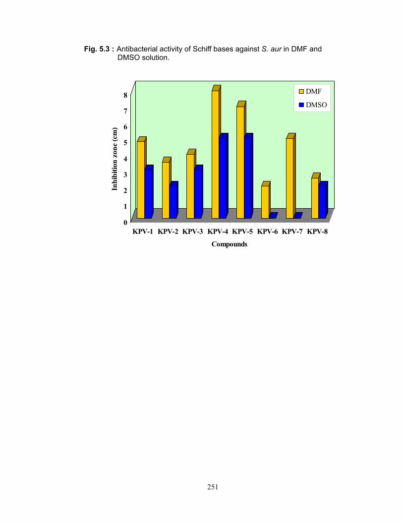
251

Fig. 5.3 : Antibacterial activity of Schiff bases against S. aur in DMF and DMSO solution.

0

1

2

3

4

5

6

7

8

Inhi

bitio

n zo

ne (c

m)


Compounds

DMF

DMSO

252

References :

[1] S. A. Khan, A. A. Siddiqui and B. Shibeer, Asian J. Chem., 14, (2002)

117.

[2] M. F. Renehan, H. J. Schanz, E. M. McGarrigle, C. T. Dalton, A. M.

Daly and D. G. Gilheany; J. Mol. Cata., A: Chemical, 231, (2005) 205.

[3] H. De Boer, A. Kool, A. Brberg, W. R. Mziray, I. Hedberg and J. J.

Levenfors, J. Ethnopharmacol, 96 (2005) 461.

[4] B. S. Holla, B. Veerendra, M. K. Shivananda and Boja, Eur. J. Med.

Chem., 38 (2003) 759.

[5] N. S. Rao and M. G. Reddy, Bio.Met., 3 (1990) 19.

[6] S. Shah, R. Vyas and R. H. Mehta, J. Ind. Chem. Soc., 69 (1992) 590.

[7] R.Shijun et al.,J.Med.Chem., 45, (2002) 410.

[8] A. H. El-Masry, H. H. Fahmy and S. H. A. Abdelwahed, Moleules, 5

(2000) 1429.

[9] P. G. More, R. B. Bhalvankar and S. C. Pattar, J. Ind. Chem. Soc., 78

(2001) 474.

[10] A. S. Khan, A. A. Siddiqui and S. A. Bhatt, Oriental J. Chem., 18 (2002)

163. [11] B. S. Holla, M. Mahalinga, M. S. Karthikeyan, B. Poojary, P.

M. Akberali and N. S. Kumari, European J. Med.Chem., 40 (2005)

1173.

[12] W. M. Singh and B. C. Dash, Pesticides, 22 (1988) 33.

[13] S. N. Pandya, D. Sriram, G. Nath and E. De Clercq, IL. Farmaco 54

(1999) 624.

[14] Abdel-Hafez O at el., Pharmazia, 48 (1993) 307.

[15] Deliwala and Chimanlal, J.Med.Chem., 14 (1971) 450.

[16] S. J. Ren, R. B. Wang, K. I. Komatsu, P. B. Krause, Y. Zgrianov, C. E.

Csipke, Z. A. Tokes and E. J. Lien, J. Med. Chem., 45 (2002) 410.

253

[17] X. Collin, J. Robert, G. Wielgosz, G. Le Baut, C. Dubigeon, N. Grimaud

and J. Petit, Eur J. Med Chem., 36 (2003) 639.

[18] M. J. Hearn and M. H. Cynamon, J. Antimicrob Chemother., 53 (2004)

185.

[19] A. K. Varshney, P. S. Verma and S. Varsheny, Synth. Rect. Met. Inorg.

Org. Chem.,19 (1989) 75.

[20] B. Dash, M. Patra and R. D. Patel, Proc.Ind.Acad.Sci., 19 (1980) 894.

[21] M. R. Manrao, R. B. Bhalvankar, R. C. Sharma, and P. S. Kalsi, J. Ind.

Chem. Soc., 73 (1996) 695.

[22] S. N. Pandya, D. Sriram, G. Nath and E. De. Clercq, Arzneimittel-

forschung., 50 (2000) 55.

[23] Y. D. Dong, J. Yan Lan and L. V. Shan, Chin. J. Chem., 19 (2001)

1136.

[24] V. V. Mulwad and J. M. Shirodkar, Ind. J. Hetrocyclic Chem., 11 (2002)

199.

[25] A. Tang, E. J. Lien and M. M. Lai, J. Med. Chem., 8 (1985) 1103.

[26] X. Ye, J. Hu, Y. Zeng, Z. Yan and J. C. Wuji, Huxaue Xuebao, 14

(1998) 84.

[27] V. E. Kuzmin, V. P. Lozitsky, G. L. Kamalov, R. N. Lozitskaya, A. I.

Zheltvay, A. S. Fedtchauk and D. N. Kryzhanovsky, Acta Biochim.

Polon., 47 (2000) 867.

[28] S. B. Desai, P. B. Desai and K. R. Desai, Hetrocycl. Commun., 7

(2001) 83

[29] R. Fioravati, M. Biava, S. Donnarumma, G. C. Porretta, N. Simonetti,

A. Villa, A. P. Port, D. Deidda, C. Maulla and R. Pompei, IL. Farmaco.,

51 (1996) 643.

[30] K. A. Shiakh, M. A. Baseer and N. A. Mote, Asian J. Chem., 13 (2001)

496.

254

[31] A. S. Chen, T. Taguchi, S. Aoyama, M. Sugiura, M. Haruna, M. W.

Wang and I. Miwa, Free Radic. Bio. Med., 35 (2003) 1392.

[32] V. V. Mulwad and J. M. Shirodkar, Ind. J. Heterocyclec Chem., 11

(2002)199.

[33] M. Bhattacharjee, B. P. Asthama, A. Kumar and D. S. Seth, J. Ind.

Chem. Soc., 69 (1992) 210.

[34] M. R. Manrao, R. K. Sethi, R. C. Sharma and P. S. Kalsi, J. Ind. Chem. Soc. ,73 (1996) 695.

[35] P. G. More, R. B. Bhalvankar and S. C. Pattar, J. Ind. Chem. Soc., 78

(2001) 474.

CHAPTER - VI

A COMPREHENSIVE

SUMMARY OF THE WORK

255

A COMPREHENSIVE SUMMARY OF THE WORK

CHAPTER – I This chapter describes the literature survey on Schiff bases

and Thiazolidinones, their characterization and physico-

chemical properties.

CHAPTER – II The synthesis of Schiff bases and thiazolidinones are

described in this chapter along with their physical constant

data.

CHAPTER – III The characterizations of all the synthesized compounds are

done by IR, NMR and mass spectral data. The spectra and

the characteristic peak positions of IR and NMR spectra are

reported. Further, mass spectra and possible fragmentation

schemes are given in this chapter.

CHAPTER – IV The physicochemical properties of some Schiff bases were

also studied and are given in this chapter. The different

properties are given in different sections.

Section : 1 In this section, heat of solution of all the Schiff bases

derived form p-amino phenol were

determined at 308.15 K in DMF and

DMSO. It is observed that the solubility of Schiff bases is

greater in DMSO than in DMF. KPV-2 shows maximum

solubility in both the solvents. However, in DMSO, KPV-5

shows minimum solubility whereas in DMF, KPV-1 exhibited

minimum solubility. The heats of solution are observed to be

positive for all the Schiff bases in both the solvents

indicating thereby endothermic behavior of these bases in

these two solvents.

Section : 2 In this section, the densities of Schiff bases were measured

in DMF and DMSO at 308.15 K. The experimental density

256

values are in good agreement with those calculated

theoretically for some cases where as in others, deviations

between theoretical and experimental densities are larger

which may be due to salvation of ions in solution.

Section : 3 This section describes the conductance of some Schiff

bases in DMF and DMSO at 308.15 K. It is observed that all

Schiff bases are weak electrolytes in nature.

Section : 4 In this section, the dissociation constants of Schiff bases in

water - dioxane mixtures are studied at 308.15 K. The acidic

character depends on the type of substituent group. It is

observed that presence of –Cl or –NO2 group at ortho

position increases the acidic character whereas at para

position, the acidic character is found to decrease. So KPV-

2 and KPV-4, showed maximum acidic character.

Section : 5 This section describes the acoustical properties of Schiff

bases in DMF and DMSO at 308.15 K. These acoustical

properties are very useful for the understanding of

interactions occurring in the solutions. It is observed that in

both DMF and DMSO solutions, except KPV-6, other bases

shows structure forming tendency. KPV-6, exhibit structure

breaking tendency in both the solvents. The nature of

groups present in Schiff base played an important role in

the predominance of the interaction.

Section : 6 The thermal properties of Schiff bases are described in this

section. DSC, TGA and DTA thermo grams were scanned

at the heating rate of 100 C per minute. Thermal stability

depends on the presence of substituent in the compound. It

is observed that KPV-2 is most stable whereas KPV-6 is

257

least stable. Various kinetic parameters such as order of

reaction, energy of activation, frequency factor and entropy

were also calculated. The negative entropy for all the

studied Schiff bases indicates the more ordered transition

state.

CHAPTER – V The antibacterial activities of some Schiff bases are

explained in this chapter. For p-amino phenol Schiff bases,

study was done in DMF and DMSO. DMF is proved to be

better solvent. The Schiff base KPV-1 with salicyldehyde

showed maximum inhibition followed by ortho and para nitro

benzaldehyde side chains (KPV-4 and KPV-5).

258

LIST OF PAPERS COMMUNICATED :

(1) Evaluation of antibacterial activity of some Schiff bases.

Shipra Baluja, j. Parekh, S. Chanda and K. P. Vaishnani.

- Croatica Chem. Acta.

(2) Dissociation constants of some Schiff bases.

Shipra Baluja, Nikunj Kachhadia, P. K. Kasundra and K. P. Vaishnani

- Institution of Chemist.

(3) Physicochemical properties of Schiff bases.

Shipra Baluja, Asif Solanki, P. K. Kasundra and K. P. Vaishnani

- J. Indian Chem. Soc.

(4) Synthesis and antimicrobial studies of some thiazolidinones.

Shipra Baluja, j. Parekh, S. Chanda and K. P. Vaishnani.

- J. Serbian Chem. Soc.

(5) Ultrasonic studies of some derivatives of p-amino phenol.


- Fluid Phase Equilibria.

(6) Molecular interaction in solutions of some Schiff bases in DMF and

DMSO.


- Physics and Chemistry of Liquids.

Documents

Saurashtra Universityetheses.saurashtrauniversity.edu/477/1/vaishnani_kp_thesis... · Medical College Rajkot, for the help in conducting biological activities. ... J. C. Javia, N