Embed Size (px)
Citation preview

Saurashtra University Re – Accredited Grade ‘B’ by NAAC (CGPA 2.93)
Bhatt, Jayeshkumar A., 2010, “Decision support system in financial statistics
for banking industries”, thesis PhD, Saurashtra University
http://etheses.saurashtrauniversity.edu/id/eprint/354
Copyright and moral rights for this thesis are retained by the author
A copy can be downloaded for personal non-commercial research or study,
without prior permission or charge.
This thesis cannot be reproduced or quoted extensively from without first
obtaining permission in writing from the Author.
The content must not be changed in any way or sold commercially in any
format or medium without the formal permission of the Author
When referring to this work, full bibliographic details including the author, title,
awarding institution and date of the thesis must be given.
Saurashtra University Theses Service
http://etheses.saurashtrauniversity.edu
© The Author

I
Decision Support System
In Financial Statistics for Banking Industries
A Thesis
Submitted To Saurashtra University, Rajkot
In Fulfilment of the Requirement for the Degree Of
Doctor of Philosophy (Statistics) In the Faculty of Science
Submitted by
Jayeshkumar Amritlal Bhatt
Under the guidance of
Dr. D. K. Ghosh
Department Of Statistics Saurashtra University, RAJKOT
(Gujarat-India)
March – 2010

II
Certificate by the Guide
This is to certify that the contents of the thesis entitled “DECISION
SUPPORT SYSTEM IN FINANCIAL STATISTICS FOR BANKING
INDUSTRIES” is the original research work of Mr. Jayeshkumar Amritlal
Bhatt carried out under my guidance and supervision.
I further certify that the work has not been submitted either partially or fully to
any other University/ Institute for the award of any degree.
Forwarded through supervisor:
Place: Rajkot Dr. D. K. Ghosh Department Of Statistics Date: 24-03-2010 Saurashtra University RAJKOT-360 005
(Gujarat-India)
Place: Rajkot Dr. D. K. Ghosh Professor and Head Date: 24-03-2010 Department Of Statistics Saurashtra University RAJKOT-360 005
(Gujarat-India)

III
Candidate’s Statement
I hereby declare that the work incorporated in the present thesis is original and
has not been submitted to any University/ Institution for the award of the
Degree. I further declare that the result presented in the thesis, considerations
made there-in, contribute in general the advancement of knowledge in
education and particular to – “Decision Support System In Financial Statistics
for Banking Industries”
Date: 24-03-2010 Jayesh Bhatt

IV
Acknowledgement
I extend my sincere thanks to Dr. D. K. Ghosh, Professor and Head,
Department of Statistics, Saurashtra University, Rajkot, who has permitted me
to work under his guidance. I take this opportunity to convey my deepest
gratitude to him for his valuable advice, encouragement, constructive criticism,
scholarly guidance and whole hearted support.
I am highly obliged by the kind hearted bank officer, who has given me the
permission and facilities to collect the data from their bank. I admire the
assistance of my friends for their help during the data collection, which is
finally used for my research work.
I have no words to express my sincere thanks to the authorities and colleagues
of my college, i.e., Gurukul Mahila Arts and Commerce College, Porbandar. I
can also not forget all the current as well as passed students who are always
praying god for the completion of my work as per my ambition and desire. I am
grateful to all the well wishers for their encouragement and again thanks them
all with due regards.
I must express my gratitude to my parents, wife Suchitra, my lovely loving
daughters Heli and Saumya without their enthusiastic and silent support, this
work could not have been completed.
Above all, I offer my heartiest regards to god for giving me patience and
strength to complete this work.
-Jayesh Bhatt
Paper Publication/ Presentation 1. A Paper: “Effect of Monthly and Daily Rest Basis on EMI for
Housing Loan” published in Spark International Online e-Journal
(Volume 2, issue 3, February- August 2010, biannual issue) at
www.sparkejournal.blogspot.com, ISSN-0979-7929-U.
2. A paper: “Effect of Rest Basis on Bank Deposits” presented in UGC
sponsored National Conference on 13th March, 2010 organized by
Department of Statistics, Saurashtra University, Rajkot (Gujarat-
India).

V
Contents
List of figures/ outputs ......................................................................................VIII
List of tables/ outputs.......................................................................................... IX
Chapter 1: Introduction..................................................................... 1-33
1.1. About Bank and Its Functions.......................................................................1
1.2. Time Series Analysis ..................................................................................11
1.3. Weibull distribution ....................................................................................19
1.4. About C/ C++ programming language.......................................................23
1.5. Objectives....................................................................................................29
Chapter 2: Research Methodology and Data Collection .............. 34-41
2.1. Data collection from bank...........................................................................34
2.2. Data preparation in excel worksheet ...........................................................35
Chapter 3: Time Series analysis ...................................................... 42-69
3.1. Introduction.................................................................................................42
3.2. Measurement of secular trend .....................................................................42
3.2.1. Freehand curve method ....................................................................42
3.2.2. Method of moving averages .............................................................49
3.2.3. Method of least squares....................................................................52
3.2.3.1. Fitting of straight line...............................................................52
3.2.3.2. Fitting of second degree curve.................................................54
3.3. Measurement of seasonal variations ...........................................................59
3.3.1. Ratio to trend method.......................................................................59
3.4. Comparison of hits and amount withdrawn ................................................63
3.5. ANOVA for hits..........................................................................................66
3.6. ANOVA for amount withdrawn..................................................................67
3.7. Mean, Median and Mode ............................................................................68

VI
Chapter 4: Effect of monthly and daily rest basis on EMI for housing, personal and car loans.................................. 70-91
4.1. Introduction.................................................................................................70
4.2. Housing loan ...............................................................................................70
4.2.1. EMI on reducing monthly rest basis ................................................70
4.2.2. EMI on reducing daily rest basis......................................................71
4.2.3. Difference of EMI on monthly & daily rest basis ............................72
4.2.4. EMI of various banks ......................................................................75
4.3. Personal loan ...............................................................................................77
4.3.1. EMI on monthly rest basis ...............................................................77
4.3.2. EMI on daily rest basis.....................................................................77
4.3.3. Difference of EMI on monthly & daily rest basis ............................78
4.3.4. EMI of various banks ......................................................................79
4.4. Car loan .......................................................................................................81
4.4.1. EMI on reducing monthly rest basis ................................................81
4.4.2. EMI on reducing daily rest basis......................................................81
4.4.3. Difference of EMI on monthly & daily rest basis ............................82
4.4.4. EMI of various banks ......................................................................83
4.5. Verification of the result .............................................................................84
Chapter 5: Effect of monthly and daily rest basis for bank deposits .............................................................. 92-107
5.1. Introduction.................................................................................................92
5.2. Methods of compounding ...........................................................................95
5.3. Calculation of maturity amount .................................................................96
5.3.1. Fixed Term Deposits ........................................................................96
5.3.2. Recurring Term Deposits ...............................................................100
5.4. Difference of policy ..................................................................................107
Chapter 6: Weibull Distribution for Amount Withdrawn per Day .................................. 108-132
6.1. Introduction...............................................................................................108
6.2. Frequency distribution of amount withdrawn per day .............................108
VII
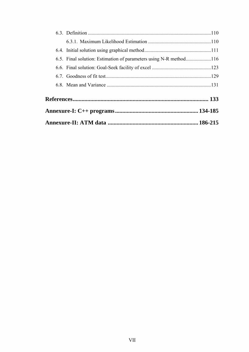
6.3. Definition ..................................................................................................110
6.3.1. Maximum Likelihood Estimation ..................................................110
6.4. Initial solution using graphical method.....................................................111
6.5. Final solution: Estimation of parameters using N-R method....................116
6.6. Final solution: Goal-Seek facility of excel ...............................................123
6.7. Goodness of fit test....................................................................................129
6.8. Mean and Variance ...................................................................................131
References............................................................................................. 133
Annexure-I: C++ programs ......................................................... 134-185
Annexure-II: ATM data .............................................................. 186-215
VIII
List of figures/ outputs
1.1 ATM ....................................................................................................................10
2.1 Sample of initial worksheet of collected data ......................................................36
2.2 Formatting of date in excel ..................................................................................38
2.3 Formatting of time in excel..................................................................................39
2.4 Sample of worksheet after conversion in numeric format ...................................40
2.5 Save as type CSV (Comma delimited) ................................................................41
3.1 Output of mmlytot.cpp, showing monthly totals .................................................47
3.2 Output of qmahit.cpp, showing quarterly moving average for hits ....................50
3.3 Output of qmaamt.cpp, showing quarterly moving average for amount .............51
3.4 Initial output of irrvartn.cpp, fitting of straight line for hits ................................52
3.5 Initial output of irramt.cpp, fitting of straight line for amount withdrawn..........53
3.6 Initial output of lsq2nd.cpp, fitting of second degree curve for hits....................55
3.7 Output of lsq2ndam.cpp, fitting of second degree curve for amount ..................57
3.8 Output of irrvartn.cpp, showing weekly trend values for hits .............................60
3.9 Output of irrvartn.cpp, showing weekly percentage of hits ................................60
and Adjusted Seasonal Indix
3.10 Output of irrvartn.cpp, showing Cyclical Irregularities.......................................61
3.11 Output of irramt.cpp, weekly total amount withdrawn........................................61
3.12 Output of irramt.cpp, showing weekly trend of amount withdrawn....................62
3.13 Output of irramt.cpp, showing weekly percentage of amount withdrawn ..........58
and Adjusted Seasonal index
3.14 Output of irramt.cpp, showing Cyclical irregularities .........................................59
3.15 Output of anovahit.cpp, showing Sum of Squares and ANOVA for hits ............66
3.16 Output of anovaamt.cpp, showing Sum of Squares and ANOVA for amount withdrawn ............................................................................................................67
4.1 Output of emimmly.cpp, showing Home loan EMI-monthly basis.....................71
4.2 Output of emidaily.cpp, showing Home loan EMI-daily basis ...........................72
4.3 Output of emidiff.cpp, showing difference of home loan EMIs.........................73
4.4 Output of emiperm.cpp, showing Personal loan EMI-monthly basis..................77
4.5 Output of emiperd.cpp, showing Personal loan EMI-daily basis ........................78
4.6 Output of emidiffp.cpp, showing difference of personal loan EMIs ..................79
4.7 Output of emicarm.cpp, showing Car loan EMI-monthly basis ..........................81

IX
4.8 Output of emicard.cpp, showing Car loan EMI-daily basis.................................82
4.9 Output of emidiffc.cpp, showing difference of car loan EMIs ............................83
4.10 Output of emicheck.cpp showing calculation of closing balance .......................87
on monthly basis
4.11 Output of emicheck.cpp showing calculation of closing balance........................90
on daily basis
4.12 Output of emichkal.cpp, showing summary of closing balances ........................91
for different tenures on monthly and daily basis
5.1 Output of fdqtrly.cpp, maturity amount for FD compounded quarterly ..............97
5.2 Output of fddaily.cpp, maturity amount for FD compounded daily ...................98
5.3 Output of fddiff.cpp, difference of maturity amounts..........................................99
List of tables/ outputs
1.1 Size and Range of data types ...........................................................................27
1.2 List of C++ programs with their brief description...........................................29
4.1 Resident home loan search results of various banks over
5, 10, 15, 20 years ............................................................................................75
4.2 Personal loan search results over 3 years.........................................................80
4.3 Car loan search results over 3 years.................................................................84
4.4 EMI check- calculation of closing balance on monthly basis (using Excel) ...86
4.5 EMI check- calculation of closing balance on daily basis (using Excel) ........88
5.1 Summary showing year wise maturity amounts and difference ......................99
5.2 Recurring deposit maturity values on compounded quarterly .......................102
5.3 Recurring deposit maturity values on compounded daily..............................103
5.4 Difference of recurring deposit maturity values ............................................104
5.5 Summary showing difference of maturity amounts for different amounts....106
6.1 Frequency distribution of amount withdrawn per day...................................108
6.2 Initial solution using graphical method..........................................................113
6.3 Final solution using N-R method...................................................................118
6.4 Final solution using goal seek facility of excel..............................................126
6.5 Summary: solutions of all methods................................................................129
6.6 Goodness of fit ...............................................................................................130
6.7 Mean of Weibull distribution.........................................................................131
6.8 Variance of Weibull distribution ...................................................................131

Chapter-1: Introduction
1
Chapter
1 Introduction
1. INTRODUCTION
Computers become more prevalent in everyday life, computer aided office practice is
fast becoming the avenue of choice for acquiring ease and accuracy in day to day life.
This can bring many benefits to human society. We can conclude that in today's
scenario computer mediated processing is the most important solution to help people
find useful information and access it in a low-cost and universal manner. This will
improve human facilities with the proper decision making for the organization as well
as people. Our aim in this thesis is therefore to cover different aspects of the banking
like loans, deposits and ATM.
1.1 ABOUT BANK AND ITS FUNCTIONS
We can say Banking is the business of providing financial services to consumers and
businesses. The basic services of a bank are checking accounts, which can be used
like money to make payments and purchase goods and services; savings accounts and
time deposits that can be used to save money for future use; loans that consumers and
businesses can use to purchase goods and services; and basic cash management
services such as check cashing and foreign currency exchange. Four types of banks
specialize in offering these basic banking services: commercial banks, savings and
loan associations, savings banks, and credit unions. A broader definition of a bank is
any financial institution that receives, collects, transfers, pays, exchanges, lends,
invests, or safeguards money for its customers. Banking services serve two primary
purposes. First, by supplying customers with the basic mediums-of-exchange (cash,
checking accounts, and credit cards), banks play a key role in the way goods and
services are purchased. Without these familiar methods of payment, goods could only
be exchanged by barter (trading one good for another), which is extremely time-
consuming and inefficient. Second, by accepting money deposits from savers and then

Chapter-1: Introduction
2
lending the money to borrowers, banks encourage the flow of money to productive
use and investments. This in turn allows the economy to grow. Without this flow,
savings would sit idle in someone’s safe or pocket, money would not be available to
borrow, people would not be able to purchase cars or houses, and businesses would
not be able to build the new factories for which the economy needs to produce more
goods and grow. Enabling the flow of money from savers to investors is called
financial intermediation, and it is extremely important to a free market economy.
1.1.1 BANKING IN INDIA
Modern banking in India is said to be developed during the British era. In the first half
of the 19th century, the British East India Company established three banks – the
Bank of Bengal in 1809, the Bank of Bombay in 1840 and the Bank of Madras in
1843. But in the course of time these three banks were amalgamated to a new bank
called Imperial Bank and later it was taken over by the State Bank of India in 1955.
Allahabad Bank was the first fully Indian owned bank. The Reserve Bank of India
was established in 1935 followed by other banks like Punjab National Bank, Bank of
India, Canara Bank and Indian Bank.
In 1969, 14 major banks were nationalized and in 1980, 6 major private sector banks
were taken over by the government. Today, commercial banking system in India is
divided into following categories. The Reserve Bank of India is the central Bank that
is fully owned by the Government. It is governed by a central board (headed by a
Governor) appointed by the Central Government. It issues guidelines for the
functioning of all banks operating within the country.
Public Sector Banks
State Bank of India and its associate banks called the State Bank Group, Other
nationalized banks and Regional rural banks mainly sponsored by public
sector banks
Private Sector Banks
Old generation private banks, new generation private banks, foreign banks
operating in India, Scheduled co-operative banks and Non-scheduled banks

Chapter-1: Introduction
3
Co-operative Sector
The co-operative sector is very much useful for rural people. The co-operative
banking sector is divided into state co-operative banks, central co-operative
banks and primary agriculture credit societies.
Development Banks/Financial Institutions
IFCI, IDBI, ICICI, IIBI, SCICI Ltd., NABARD, Export-Import Bank of India,
National Housing Bank, Small Industries Development Bank of India and
North Eastern Development Finance Corporation.
1.1.2 FUNCTIONING OF A BANK
Functioning of a Bank is among the more complicated of corporate operations. Since
Banking involves dealing directly with money, governments in most countries
regulate this sector rather stringently. In India, the regulation traditionally has been
very strict. This section, which is also intended for banking professional, attempts to
give an overview of the functions in as simple manner as possible.
Banking Regulation Act of India, 1949 defines Banking as "accepting, for the purpose
of lending or investment of deposits of money from the public, repayable on demand
or otherwise and withdrawable by cheques, draft, order or otherwise."
Deriving from this definition and viewed solely from the point of view of the
customers, personal banking, Banks essentially perform the following functions:
1.1.2.1 ACCEPTING DEPOSITS FROM PUBLIC/ OTHERS
1.1.2.1.1 TERM DEPOSIT
Now one can earn a higher income on the surplus funds by investing those with bank.
Bank provides security, trust and competitive rate of interest. It is having flexibility in
period of term deposit from 15 days to 10 years (generally) and affordable low
minimum deposit amount.
1.1.2.1.2 RECURRING DEPOSIT
One can create fund for future planning by investing/ depositing monthly basis.
Whatever may be the financial goals, through Recurring Deposit Scheme, one can

Chapter-1: Introduction
4
save a little amount every month so that at the time of need one will have sufficient
funds to achieve financial goals. Recurring Deposit provides the element of
compulsion to save at high rates of interest applicable to Term Deposits along with
liquidity to access that savings any time. So it is the deposit to set aside a small
amount every month and earn at compounded (quarterly) rates of interest.
Flexibility in period of deposit with maturity ranging from 12 months to 120
months.
Low minimum monthly deposit amount.
1.1.2.2 LENDING MONEY TO PUBLIC (LOANS)
Lending money is one of the two major activities of any Bank. In a way, the Bank
acts as an intermediary between the people who have the money to lend and those
who have the need for money to carry out business transactions. Landing money to
public is in form of various types of loans like Housing loan, Personal loan, Education
loan, Car loan, Loan against mortgage of property etc. Some of the few loans are
given below:
1.1.2.2.1 HOUSING LOAN
This can be utilised for purchase/ construction of house/ flat, purchase of a plot of
land for construction of house, extension/ repair/ renovation/ alteration of an existing
house/ flat, purchase of furnishings and consumer durables as a part of the project cost
and takeover of an existing loan from other banks/ housing finance companies.
Most of the friends or relatives I know here in surrounding area has either already
bought a house or are planning to buy one. The biggest incentives are perhaps the
easy availability of home loans at interest rates far lower than that available to the
previous generation and the tax-breaks one gets here in India on the principal and the
interest paid on home loans. Our generation is also not averse to taking on a debt
unlike the previous generation. In addition, many of us feel that it is better to take the
plunge now and enjoy the comforts of your own house than to diligently save all the
required money for years and then buy a house, only to find out that the dream was
realised a bit too late in your life.

Chapter-1: Introduction
5
1.1.2.2.2 REDUCING BALANCE LOAN
Suppose you took a Rs 1 lakh loan today at a rate of interest of 10 per cent for five
years. You are to pay back Rs 20,000 of the principal and Rs 10,000 (10 per cent of
the loan) every year. So you pay back Rs 30,000 every year. Over five years you pay
back Rs 1.5 lakh. But notice, that the loan kept reducing over the five years as you
paid back Rs 20,000 each year, yet you went on paying interest for five years, as if
you had kept the Rs 1 lakh for the entire term.
What if you paid an interest only on the amount you owed each year and not the entire
one lakh?
The first year you would pay Rs 10,000 as interest, the next year you would pay Rs
8,000 on a reduced principal of Rs 80,000 and so on, till the last year, you pay only Rs
2,000 as interest. Now you would have paid back Rs 1.3 lakh instead of Rs 1.5 lakh as
in the earlier case.
The first case is a situation of a loan that charges interest at a flat rate and the second
case is when the interest is calculated on a ‘reducing balance’ or only on the amount
of loan left to pay and not the entire loan amount. A flat 10 per cent is nearly equal to
a reducing balance at 6 per cent per annum.
You can get a range of options in reducing balance loans. You get annual, quarterly,
monthly, weekly and now daily rests. A ‘rest’ is jargon to indicate when the bank will
recalculate the EMI based on the amount of loan paid back. Suppose you have a loan
with an annual ‘rest’ then, though you pay a monthly instalment, your benefit kicks in
only at year end. Meaning the bank gets free interest for 11 months. A monthly ‘rest’
will recognise the reduction in the loan amount on a monthly basis and a daily ‘rest’
will do it each day.
1.1.2.2.3 CALCULATING EMIS
When one takes a loan, a natural question that comes to mind is how much the EMI
(Equated Monthly Instalment) would be that one has to pay back to the bank every
month. Finding out the EMI for different tenures of the home loan allows one to select
the best tenure based on one's current and projected income and expenses and
possibly other factors.
Chapter-1: Introduction
6
What I find is that most friends would rather use a bank’s EMI calculator rather than
calculating it themselves. Some brave souls ask around for the formula to calculate
EMIs and then try to write a programme that calculates the EMIs for them. I find it
particularly appalling that very few bother to figure it out for themselves, especially
since it involves elementary algebra that most of us have surely learnt in high school.
It either reflects the creeping sloth and sloppiness in our generation or the rote
learning and regurgitating of formulae that our system of education seems to
encourage. In any case, I attempt to show how simple it really is to figure out how to
calculate EMIs on your own and the effect of monthly rest basis and daily rest basis
on it using C++ programming.
For the sake of simplicity, assume that the loan is offered on a "monthly rest" basis.
That is, the bank calculates the interest at the end of every month on the amount you
still owe to the bank at the beginning of the month, adds it to the amount you already
owe and then deducts your EMI from this to calculate the total amount you still owe
to the bank at the beginning of the next month. Most of all banks offer loans on a
"daily rest" basis, where the outstanding amount and the interest is recalculated every
day, but you still pay back on a monthly basis.
Formula of EMI for “monthly rest basis”
Suppose you take on a loan for P Rupees, the tenure of the loan is n months (for
example, n=240 for a 20-year loan), the monthly rate of interest is r (usually
calculated by dividing the annual rate of interest quoted by the bank by 12, the
number of months in a year, and dividing that by 100 as the rate is usually quoted as a
percentage) and EMI Rupees is the EMI you have to pay every month.
Let us use P(i) to denote the amount you still owe to the bank at the end of the ith
month. At the very beginning of the tenure, i=0 and P(0)=P, the principal amount you
took on as a loan.
At the end of the first month, you owe the bank the original amount P, the interest
accrued at the end of the month r×P and you pay back EMI. In other words:
EMIPrPP 1 or to rewrite it slightly differently EMIrPP 11
Similarly, at the end of the second month the amount you still owe to the bank is:
EMIrPP 112 or substituting the value of P(1) we calculated earlier:

Chapter-1: Introduction
7
EMIrEMIrPP 112
and once again expanding it and rewriting it slightly differently:
1112 2 rEMIrPP (1.1)
The term "xy" denotes "x raised to the power y" or "x multiplied by itself y times". To
make this look slightly simpler, we substitute "(1 + r)" in equation-(1) by "t" and now
it looks like this:
P(2) = P×t2 - EMI×(1 + t)
Continuing in this fashion and calculating P(3), P(4) etc. we quickly see that P(i) is
given by:
P (i)= P×ti - EMI×(1 + t + t2 + ... + ti-1)
At the end of n months (that is, at the end of the tenure of the loan), the total amount
you owe to the bank should have become zero. In other words, Pn=0. This implies
that:
P(n) = P×tn - EMI×(1 + t + t2 + ... + tn-1) = 0, which means that:
P×tn = EMI×(1 + t + t2 + ... + tn-1) (1.2)
We can simplify this further by noticing that we have a geometric series of n terms
here with a common ratio of t and a scale factor of 1.
The sum of such a series is given by "(tn - 1)/(t - 1)", which we substitute in the above
equation-(2) to yield:
P×tn = EMI×(tn - 1)/(t - 1), which can be rewritten as:
EMI = P×tn×(t - 1)/(tn - 1) (1.3)
Equation (3) can again be rewritten by substituting the value of t back as "(1 + r)" as:
EMI = P×r×(1 + r)n/((1 + r)n - 1) (1.4)
and this is the formula for calculating your EMI.
1.1.2.2.4 EDUCATION LOAN
A term loan granted to Indian Nationals for pursuing higher education in India or
abroad where admission has been secured. There will be Comparatively higher
interest rates than Housing loan.
Chapter-1: Introduction
8
Eligible Courses
All courses having employment prospects are eligible, such as graduation courses/
post graduation courses/ professional courses and other courses approved by UGC/
government/ AICTE etc.
Expenses considered for loan
Fees payable to college/school/hostel, Examination/Library/Laboratory fees, Purchase
of Books/Equipment/Instruments/Uniforms, Caution Deposit/Building Fund/
Refundable Deposit (maximum 10% tuition fees for the entire course), Travel
Expenses/Passage money for studies abroad, Purchase of computers considered
necessary for completion of course and cost of a two-wheeler up to Rs. 50,000/- are
expenses considered for loan.
1.1.2.2.5 PERSONAL LOAN
Do you want funds readily available to you whenever you desire or need, be it a
sudden vacation that you plan with your family or urgent funds required for medical
treatment? Personal Loan is the answer to your questions. The loan will be granted for
any legitimate purpose whatsoever (e.g. expenses for domestic or foreign travel,
medical treatment of self or a family member, meeting any financial liability, such as
marriage of son/daughter, defraying educational expenses of wards, meeting margins
for purchase of assets etc.) It is having comparatively higher interest rates. Repayment
terms generally up to 4-5 years.
1.1.2.3 TRANSFERRING MONEY FROM ONE PLACE TO ANOTHER
(REMITTANCES)
Apart from accepting deposits and lending money, Banks also carry out, on behalf of
their customers the act of transfer of money - both domestic and foreign.- from one
place to another. This activity is known as "remittance business". Banks issue
Demand Drafts, Banker's Cheques, Money Orders etc. for transferring the money.
Banks also have the facility of quick transfer of money also know as Telegraphic
Transfer or Tele Cash Orders.
Chapter-1: Introduction
9
1.1.2.4 ACTING AS TRUSTEES
Banks also act as trustees for various purposes. For example, whenever a company
wishes to issue secured debentures, it has to appoint a financial intermediary as trustee
who takes charge of the security for the debenture and looks after the interests of the
debenture holders. Such entity necessarily have to have expertise in financial matters
and also be of sufficient standing in the market/society to generate confidence in the
minds of potential subscribers to the debenture.
1.1.2.5 KEEPING VALUABLES IN SAFE CUSTODY
Bankers are in the business of providing security to the money and valuables of the
general public. While security of money is taken care of through offering various type
of deposit schemes, security of valuables is provided through making secured space
available to general public for keeping these valuables. These spaces are available in
the shape of LOCKERS. The latter are small compartments with dual locking facility
built into strong cupboards. These are stored in the Bank's Strong Room and are fully
secure. Lockers can neither be opened by the hirer or the Bank individually. Both
must come together and use their respective keys to open the locker.
1.1.2.6 GOVERNMENT BUSINESS
Earlier Government business used to be exclusively carried out by Governement
Treasuries where all type of transactions took place. However, now Banks act on
behalf of the Government to accept its tax and non tax receipts. Most of the
Government disbursements like pension payments and tax refunds also take place
through banks. While the Banks carry out this business for a fee to be paid by the
Government,
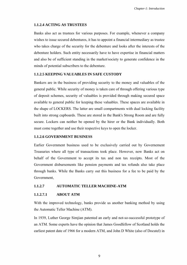
1.1.2.7 AUTOMATIC TELLER MACHINE-ATM
1.1.2.7.1 ABOUT ATM
With the improved technology, banks provide us another banking method by using
the Automatic Teller Machine (ATM).
In 1939, Luther George Simjian patented an early and not-so-successful prototype of
an ATM. Some experts have the opinion that James Goodfellow of Scotland holds the
earliest patent date of 1966 for a modern ATM, and John D White (also of Docutel) in

Chapter-1: Introduction
10
the US is often credited with inventing the first free-standing ATM design. In 1967,
John Shepherd-Barron invented and installed an ATM in a Barclays Bank in London.
FIGURE 1.1 ATM
Don Wetzel invented an American made
ATM in 1968. However, it wasn't until
the mid to late 1980s that ATMs became
part of mainstream banking.
The Automatic teller machine is good
because it helps solve problems for
people who don’t have time to stand in
line waiting inside the bank, or who don’t
have patience of getting help from the
tellers who are performing a slow job at
the drive-through window. In order for a
customer to make a deposit, you don’t
need to go inside the bank, but you can
still deposit it at any time at the ATMs
because it has unlimited hours of
operations and there will be a limit of
cash that will be available for you to
withdraw for the next hours after you deposit. It is also good for people who are
traveling around the world, they don’t need to carry their cash in their hands, or find
their bank locations in order to withdraw cash. It also give you access to your savings
account. The ATM machine always provides the sign of card logo’s that it accepts
before you can insert your card. If you are a non bank customer of a particular that
ATM’s bank machine, there is a specific fee amount that the bank will charge you in
order for you to proceed for further request. For several years, ATM banking services
have made it easy for customers to bank without worries. As technology keep on
improving, there will be more and more ways that banks will attract people to do
business with them. Bankers would still need to be careful with scam, and need to
protect their identifications. This banking system will improve even more in years to
come.
Chapter-1: Introduction
11
1.1.2.7.2 TRANSACTIONS USING AN ATM CARD
You can conduct the common transactions like deposits, withdrawals, balance
inquiries, mini statements, change your PIN etc. at ATM locations (some transaction
types are not available at all ATM locations):
1.1.2.7.3 LIMITATIONS OF ATMS
Customer can not decide the denominations of notes. Customer can get the
notes in predefined denominations. i.e., if amount is more than Rs. 500 then
customer will get 5 or less notes of Rs. 100 and remaining notes of Rs. 500.
Upper limit of withdraw the money per day is fixed by the bank (ranging Rs.
15000 to 40000), so the customer can not utilise the available balance fully.
Customer can not get the money if the ATM is not loaded with the money.
Customer can not get the money if the machine is faulty or power supply or
link is down.
Cracking the PIN and card duplication will harm the customer.
1.2 TIME SERIES ANALYIS
A time series is a set of measurements on a variable taken over some period of time.
The time frame of the recorded data may be an hour, a day, a week , a month, a year
of a fixed number of years, depending upon the type of event the data refer to. For
example, hourly temperature of a particular city, weekly earnings of workers in an
industrial town, monthly prices of wheat. Most forecasting techniques involve the use
of time series data. In a simple analysis, a time series is assumed to contain the
following components.
1.2.1 COMPONENTS
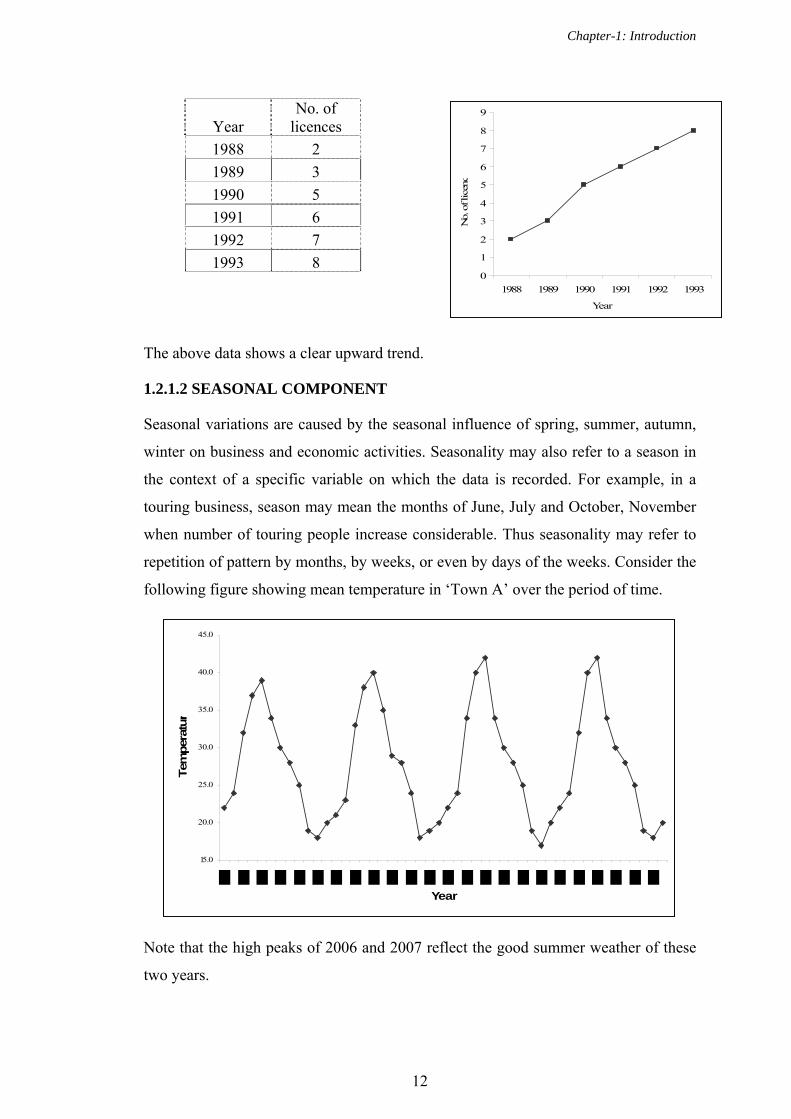
1.2.1.1 THE TREND (SECULAR TREND)
Trend is the long-term tendency of the time series to move in an upward or downward
direction. It can be defined as, “A consistent long term change in the average level of
the forecast variable per unit of time”. Consider the following figure showing the data
on the colour TV licences issued over the period of time.
Chapter-1: Introduction
12
The above data shows a clear upward trend.
1.2.1.2 SEASONAL COMPONENT
Seasonal variations are caused by the seasonal influence of spring, summer, autumn,
winter on business and economic activities. Seasonality may also refer to a season in
the context of a specific variable on which the data is recorded. For example, in a
touring business, season may mean the months of June, July and October, November
when number of touring people increase considerable. Thus seasonality may refer to
repetition of pattern by months, by weeks, or even by days of the weeks. Consider the
following figure showing mean temperature in ‘Town A’ over the period of time.
15.0
20.0
25.0
30.0
35.0
40.0
45.0
Year
Tem
per
atur
Note that the high peaks of 2006 and 2007 reflect the good summer weather of these
two years.
Year No. of
licences
1988 2
1989 3
1990 5
1991 6
1992 7
1993 8 0
1
2
3
4
5
6
7
8
9
1988 1989 1990 1991 1992 1993
Year
No.
of l
icen
c
Chapter-1: Introduction
13
1.2.1.3 THE CYCLICAL COMPONENT
Cyclical variations, which are also generally termed as business cycles, are the
periodic movements in the time series around the trend line. These are the upswings
and downswings in the time series that are observable over extended periods of time.
Neither the magnitude nor the frequency of occurrences of these cycles is uniform.
For example, A high boom in the stock market in India for a span of four-five years in
1990’s caused by the Harshad Mehta factor, can be considered as a cyclical
component erecting the activity level of stock market over a period of time.
The cyclical fluctuations are like waves which come and go. At times the cyclical
waves prevails for a very long period of time, say 50 years, but these long waves are
difficult to be distinguished as they get mixed up with the trend line.
1.2.1.4 THE ‘IRREGULAR’ OR ‘DISTURBANCE’ COMPONENT
This is taken to be a random, non systematic component, affecting the time series
through such unpredictable events as strikes, breakdown of plant, non-seasonal
illness, bad weather etc. These variations either go very deep downward or too high
upward to attain peaks abruptly. These do not occur frequently and are less important
than the cyclical or seasonal movements.
1.2.2 MODELS OF TIME SERIES ANALYSIS
Analysis of time series involves decomposition of time series into its four components
listed above. The objective is to estimate and separate the four types of variations and
to bring out the relative impact of each on the overall behaviour of the time series.
There are two models of decomposition of time series:
(i) the additive model (ii) the multiplicative model
1.2.2.1 THE ADDITIVE MODEL
This model is used where it is assumed that the four components are independent of
one another. Independence is said to exist when the pattern of occurrences and the
magnitude of movements is any particular component are not affected by the other
components. Under this assumption, the four components are arithmetically additive
in the sense that magnitudes of the time series are the sum of the separate influences
of its four components. Thus, if it is taken to represent the magnitude of the time
series data at time period t, then Yt can be expressed as:

Chapter-1: Introduction
14
Yt = Tt + Ct + St + Rt
Where Tt represents Trend variations, Ct represents Cyclical variations, St represents
Seasonal variations and Rt represents Random variations
1.2.2.2 THE MULTIPLICATIVE MODEL
This model is used where it is assumed that the forces giving rise to the four types of
variations are independent, so that overall pattern of variations in the time series is the
combined result of the interaction of all the forces operating on the time series.
According to this model, time series are the product of its four components, that is
Yt = Tt x Ct x St x Rt
As regards the choice between the two models, it is generally the multiplicative model
which is used more frequently. The reason being that most business and economic
time series data are the result of interaction of a large number of forces which,
individually, cannot be treated responsible for generating any particular type of
variations. Since the forces responsible for one type of variations are also responsible
for the other types of variations, it is the multiplicative model which is ideally suited
for the purpose of decomposition of a time series.
1.2.3 MEASUREMENT OF SECULAR TREND
The trend is a concept defining long-term. It does not include short-run oscillations
but indicates the steady movements of the variable over a long period of time. But
when we record a time series data on a variable, it includes short-run oscillations also.
Thus, for measuring the trend values, we first smoothen the data to remove short-term
oscillations. For such smoothing any of the following methods may be used:
1. Freehand curve method 2. Method of semi-averages
3. Method of moving averages 4. Method of least squares
1.2.3.1 FREEHAND CURVE METHOD
First we draw a curve after plotting the data of a given time series. It will be irregular
as it would include short-run oscillations. We may observe the up and down
movement of the curve and smooth out the irregularities by drawing a freehand curve
or line along with the curve previously drawn. This freehand curve would eliminate
Chapter-1: Introduction
15
the short-run oscillations and show the long-period general tendency of the data. This
is exactly what is meant by trend.
Note this method has serious disadvantage that different persons may draw the
freehand line at different positions and with different slopes. There is, therefore, the
danger of different conclusions being draw by different persons.
1.2.3.2 METHOD OF SEMI-AVERAGES
Under this method the whole series is divided into two equal halves and the averages
for each half are calculated. If the data is for even number of years, it can easily be
divided into two halves. But if it is for odd number of years, we leave the middle year
of the time series and two halves constitute the periods on each side of the middle
year.
The average for a half is taken to be representative of the value corresponding to the
mid point of the time interval of that half. We, thus, get two points. These two points
are plotted on a graph and are joined by straight line which provides us the required
trend line.
This method is a more objective approach than the free-hand method. But this method
is not completely free from criticism. Because we used the mean of each half of the
series, any extreme item will greatly affect the points. Such a trend may not be an
accurate picture of the growth element in the series. In addition, values so obtained
are not precise enough for predictive purpose or for the trend elimination.
1.2.3.3 METHOD OF MOVING AVERAGES
A moving average is an average of fixed number of items in a series which moves
through the series by dropping the top item of the previous averaged group and adding
the next item below in each successive average. Thus a moving average is computed
by adding all the values for a certain number of successive periods and then dividing
the sum which is obtained by the number of periods included. This average is
considered as the trend value for the unit of time falling at the centre of the period
used in the calculation of the average. To compute three yearly moving average, for
instance, the values of 1st, 2nd and 3rd years are added up, averaged and the quotient is
placed against the 2nd year; then values of the 2nd, 3rd and 4th years are added up,
averaged and the average is placed against the 3rd year; and so on.

Chapter-1: Introduction
16
The moving averages series would yield a smooth curve, provided the time interval
chosen for computing the moving average is appropriate. Moving averages may be
calculated for odd number of years like 3 years moving average, 5 years moving
average, 7 years moving average and for even number of years like 4 years moving
average, 6 years moving average and so on. In the case of odd numbers moving
average, we place the average against the central year, but when period is even, we
follow the ‘method of centering’.
The method of moving averages is simple and free from personal bias of the estimator
but the choice of the period of moving average needs a great care. If an inappropriate
period is selected, a true picture of the trend cannot be obtained. Moreover it involves
use of arithmetic average which gets affected by extreme values of the data.
1.2.3.4 METHOD OF LEAST SQUARES
The method of least squares may be used either to fit a linear trend or a non-linear
trend. Under this method, a mathematical relationship is established between the time
factor X and the variable Y, A straight line of trend is obtained by using the equation
for a straight line, which is Yt = a + bX.
Where the value of ‘a’ is merely the Y-intercept or the height of the line above origin.
That is, when X=0, Y=a. The other constant ‘b’ represents the slope of the trend line.
When b is positive, the slope is upwards, and when b is negative, the slope is
downward.
This line is termed as the line of best fit because it is so fitted that the total distance of
deviations of the given data from the line is minimum. The total of deviation is
calculated by squaring the difference in trend value and actual value of a variable.
Thus, the term “least squares” is attached to this method.
To estimate the value of the constants in the above equation, we start with normal
equations. The following are the two normal equations for fitting a straight line by the
method of least squares:
)()( xbnay
2)()()( xbxaxy
Chapter-1: Introduction
17
1.2.4 MEASUREMENT OF SEASONAL VARIATIONS
The effects of trend cycles and irregular fluctuations must be eliminated from the
original time series data to obtain an estimate of seasonal variation. Once they are
eliminated, we get measures of seasonal variations in the behaviour of any variable.
These measures are called seasonal indexes. By using such indexes, we can
deseasonalise the time series. Such deseasonalised data are known as seasonally
adjusted data.
There are four methods of constructing seasonal index:
1. Method of Simple Averages 2. Ratio-to-Trend Method
3. Moving Average Method 4. Link Relatives Method
1.2.4.1 METHOD OF SIMPLE AVERAGES
This is the simplest method of obtaining a seasonal index. The following steps are
required to calculate index:
(i) Arrange the unadjusted data by months and weeks (say, quarters)
(ii) Find the totals of all quarters for January, February, etc.
(iii) Divide each total by the number of months for which data are given and get
quarterly average.
(iv) Obtain general average of quarterly/weekly averages.
(v) Compute seasonal index as follows:
100average General
quarter1st for averageQuarterly quarter 1st for Index Seasonal
This method is simplest of all the methods of estimating the seasonal variations. But it
is not a scientific method. The computation is based on the assumption that there is no
trend component in the given time series. Thus the resultant seasonal index is a
combination of trend and seasonal variations.
1.2.4.2 RATIO TO TREND METHOD
This method isolates the seasonal factor after eliminating the trend from tie series.
Trend is eliminated by computing the ratios, and random elements disappear when the
ratios are averaged. The steps involved in computation of index are:

Chapter-1: Introduction
18
1. Determine trend value by the method of least squares.
2. Divide the original data quarter by quarter, by the corresponding trend values
and express them as percentages.
3. Average the different values for a quarter.
4. Adjust all these averages.
It may be noted here that step (2) eliminates the trend and the values so obtained
include cyclical and irregular variations. Step (3) frees the values from cyclical and
irregular variations.
1.2.5 MEASUREMENT OF CYCLICAL VARIATIONS: Residual Method
Since the original data are represented by tttt RCST we can obtain the cyclical
irregular movements by eliminating trend and seasonal variation, that is
tttt
tttt RCST
RCST
The remaining data RC are usually smoothed out to obtain the cyclical variations,
which are called the cyclical relatives or percentages. This is done by the method of
moving averages, and the irregular component is removed in the process of averaging.
As a result, what is left in the series is merely the cyclical movements. This explains
why the procedure is commonly referred to as the residual method. Steps are:
1. Multiply the trend values by seasonal index.
2. The original figures of the time series are divided by resultant products,
resulting in the combination of the cyclical and irregular movements.
3. For smoothing out irregular movement from tt RC data, obtain moving
average from the tt RC data.
4. C is left as a residue.
1.2.6 MEASUREMENT OF IRREGULAR VARIATIONS
The irregular component in a time series represents the residue of fluctuations after
trend, cyclical and seasonal movements have been accounted for. It may be
represented as follows:

Chapter-1: Introduction
19
tttt
tttt
ttt
RSCT
RSCT
SCT
Y
It is simple to measure the irregular fluctuations, once the trend, seasonal and cyclical
variations have been measured.
1.3 WEIBULL DISTRIBUTION
This distribution is found to be of great importance in the fields of reliability and life
testing. Perhaps this is the most widely used life time distribution. As early as 1928
researchers in the theory of extreme value knew this distribution to which the name
weibull is given. This distribution had been derived earlier by Fisher and Tippett
(1928). This is also known as Fisher-Tippett type III distribution. The Weibull
distribution arises in a natural way from the exponential distribution if we assume that
βth power of failure time has exponential distribution. Weibull (1951) showed this
distribution is useful in decreasing the ‘wear out’ or fatigue failures. The work may be
classified under the various categories as follows:
1.3.1 DEFINITION
The life time random variable x is said to have Weibull distribution if its probability
density function is given by
x
xxf exp,, 1 where x>0, >0, >0 (1.3.1)
β is the shape parameter and θ is the scale parameter, which is known as two-
parameter Weibull distribution.
1.3.2 MAXIMUM LIKELIHOOD ESTIMATION
Cohen (1965) suggested the following method by which we can obtain Maximum
Likelihood Estimates of β and θ by means of iterative procedure.
Let x1, x2, x3, …, xn be a random sample of size n from w(0, β, θ) distribution. The
Likelihood function of this sample is
L(x1, x2, x3, …, xn; β θ)=
in
ii
xx exp
1
1
Taking logarithm we get

Chapter-1: Introduction
20
Ln L= n ln β – n ln θ + (β-1)
n
iin
ii
xx 1
1
ln (1.3.2)
Differentiating log likelihood with respect to the parameters β and θ and equating to
zero we obtain
0ln
lnln
1
1
n
i
n
iii
i
xxx
nL
(1.3.3)
0ln
21
n
i
xnL
(1.3.4)
n
ii
n
iii
x
xxnnL
1
1
2
22
2ln
ln
(1.3.5)
n
iix
nL
1322
2 2ln
(1.3.6)
n
iii xx
LL
12
22
ln1lnln
(1.3.7)
ˆ,ˆ2
22
2
2
2
lnln
lnln
LL
LL
EI (1.3.8)
1 IE
ˆˆ
lnˆˆ
lnˆln
ˆln 22
2
2
2
2 LE
LE
LE
LEK
ˆ,ˆ2
22
2
2
2
lnln
lnln
1
LE
LE
LE
LE
K

Chapter-1: Introduction
21
1.3.3 GRAPHICAL METHOD OF GETTING INITIAL SOLUTION
We have,
ty
xxF
xxF
xxF
exFx
lnlnlnln
ln
ln
Where, t=ln x and = -ln
For given data x1, x2, x3, …, xn we obtain ti=ln xi, i=1,2,3,…. (1.3.9)
The survival function xF is calculated using Kaplan-meier estimator as
1
1ˆ
n
inxF i
Define si )(lnln( )(ixF
))1
1ln(ln(
in
n (1.3.10)
By taking (si, ti), i=1, 2, 3, …, n we fit a straight line.
Then estimator of slope (which is same as shape parameter)
2)(
))((ˆtt
ttss
i
ii (1.3.11)
And
)(,)(
)(,
ˆ
)(
ˆ
censoredr
xrnx
uncensoredn
x
ri
i
(1.3.12)
Chapter-1: Introduction
22
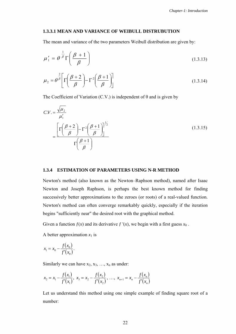
1.3.3.1 MEAN AND VARIANCE OF WEIBULL DISTRUBUTION
The mean and variance of the two parameters Weibull distribution are given by:
1
1
1 (1.3.13)
12 2
2
2 (1.3.14)
The Coefficient of Variation (C.V.) is independent of θ and is given by
1
12
..
21
2
1
2VC
(1.3.15)
1.3.4 ESTIMATION OF PARAMETERS USING N-R METHOD
Newton's method (also known as the Newton–Raphson method), named after Isaac
Newton and Joseph Raphson, is perhaps the best known method for finding
successively better approximations to the zeroes (or roots) of a real-valued function.
Newton's method can often converge remarkably quickly, especially if the iteration
begins "sufficiently near" the desired root with the graphical method.
Given a function ƒ(x) and its derivative ƒ '(x), we begin with a first guess x0 .
A better approximation x1 is
0
001 xf
xfxx
.
Similarly we can have x2, x3, …, xn as under:
1
112 xf
xfxx
,
2
223 xf
xfxx
, …,
n
nnn xf
xfxx
1
Let us understand this method using one simple example of finding square root of a
number:

Chapter-1: Introduction
23
If we wish to find the square root of 5, this is equivalent to find the solution to
52 x ,
So, the function used in N-R method is then
52 xxf
With derivative xxf 2
With an initial guess of 20 x , the sequence of iteration to find the solution given by
N-R method is as under:
0
001 xf
xfxx
= 22
522
2 = 2.25
1
112 xf
xfxx
= 25.22
525.225.2
2 =2.2361111111
2
223 xf
xfxx
= 112.236111112
5112.23611111112.23611111
2 =2.2360679779
3
334 xf
xfxx
= 792.236067972
5792.23606797792.23606797
2 =2.2360679774
4
445 xf
xfxx
= 742.236067972
5742.23606797742.23606797
2 =2.2360679774
It is quite remarkable that the results stabilize for ten decimal places after only 5
iterations!
1.4 ABOUT C/ C++ PROGRAMMING LANGUAGE
In computing, C is a general-purpose, block structured, procedural, imperative
computer programming language developed in 1972 by Dennis Ritchie at the Bell
Telephone Laboratories for use with the Unix operating system.
Although C was designed for implementing system software, it is also widely used for
developing application software.
It is widely used on a great many different software platforms and computer
architectures, and several popular compilers exist. C has greatly influenced many
Chapter-1: Introduction
24
other popular programming languages, most notably C++, which originally began as
an extension to C.
1.4.1 EARLY DEVELOPMENTS
The initial development of C occurred at AT&T Bell Labs between 1969 and 1973;
according to Ritchie, the most creative period occurred in 1972. It was named "C"
because many of its features were derived from an earlier language called "B", which
according to Ken Thompson was a stripped-down version of the BCPL programming
language.
The origin of C is closely tied to the development of the UNIX operating system,
originally implemented in assembly language on a PDP-7 by Ritchie and Thompson,
incorporating several ideas from colleagues. Eventually they decided to port the
operating system to a PDP-11. B's lack of functionality to take advantage of some of
the PDP-11's features, notably byte addressability, led to the development of an early
version of the C programming language.
The original PDP-11 version of the Unix system was developed in assembly
language. By 1973, with the addition of struct types, the C language had become
powerful enough that most of the UNIX kernel was rewritten in C. This was one of
the first operating system kernels implemented in a language other than assembly.
Short history of the C family of languages is as under:
1972 - The precursor to C, the language B, is developed at Bell Labs. The B
language is fast, easy to maintain, and useful for all kinds of development
from systems to applications. The entire team that designed the language is
immediately fired for behavior unbefitting a telephone company employee,
and the project is handed to Dennis Ritchie. He alters the language to be
incomprehensible, difficult to maintain, and only useful for systems
development. He also designs in a pointer system guaranteed to give every
program over 500 lines a pointer into the operating system.
1982 – It is discovered that 97% of all C routine calls are subject to buffer overrun
exploits. C programmers begin to realize that initializing a variable to
whatever happens to be lying around in memory is not necessarily a good
Chapter-1: Introduction
25
idea. However, since enforcing sensible variable initialization would break
97% of all C programs in existence, nothing is done about it.
1984 – The number of operating systems has been dramatically increased.
1985 – A variant of C with object oriented capabilities, called C With Classes, is
ready to go commercial. However, the name C With Classes is considered
too clear and easy for outsiders to understand, so the commercial version is
called C++.
1986 – C becomes so popular that industry analysts recommend writing business
applications in it. They argue that applications written in C will be portable to
many different systems. Many of these industry analysts are suspected of
being under the influence of hallucinogens.
1988 – Industry analysts finally run out of LSD. After their hallucinations fade, they
notice that business apps written in C take five times longer to produce, and
are still not portable. They stop recommending that business apps be written
in C, except for a minority that switch to crack cocaine and start
recommending business apps be written in C++ because “object orientation
will result in code reuse”.
By this time, all C compilers have turned into C++ compilers and we can say C is a
subset of C++, here we have also used C++ compiler.
1.4.2 DATA TYPES
As a programming language, C is rather like Pascal or Fortran. Values are stored in
variables. Programs are structured by defining and calling functions. Program flow is
controlled using loops, if statements and function calls. Input and output can be
directed to the terminal or to files. Related data can be stored together in arrays or
structures. Of the three languages, C allows the most precise control of input and
output. C is also rather more terse than Fortran or Pascal. This can result in short
efficient programs, where the programmer has made wise use of C's range of powerful
operators. It also allows the programmer to produce programs which are impossible to
understand.
Care must be taken in using C. Many of the extra facilities which it offers can lead to
extra types of programming error. While dealing with large real numbers we should

Chapter-1: Introduction
26
be very careful for their data type and range. Let us have a brief understanding about
data types available in C. Here we will have brief note about data types, Primary data
type, Integer Type, Floating Point Types, Void Type, Character Type, Size and Range
of Data Types on 16 bit machine. A C language programmer has to tell the system
before-hand, the type of numbers or characters he is using in his program. These are
data types. There are many data types in C language. A C programmer has to use
appropriate data type as per his requirement. Data types available in C language are
like:
1.4.2.1 INTEGER TYPES
Integers are whole numbers with a machine dependent range of values. A good
programming language supports the programmer by giving a control on a range of
numbers and storage space. C has 3 classes of integer storage namely short int, int and
long int. All of these data types have signed and unsigned forms. A short int requires
half the space than normal integer values. Unsigned numbers are always positive and
consume all the bits for the magnitude of the number. The long and unsigned integers
are used to declare a longer range of values.
1.4.2.2 FLOATING POINT TYPES
Floating point number represents a real number with 6 digits precision. Floating point
numbers are denoted by the keyword float. When the accuracy of the floating point
number is insufficient, we can use the double to define the number. The double is
same as float but with longer precision. To extend the precision further we can use
long double which consumes 80 bits of memory space.
1.4.2.3 VOID TYPE
Using void data type, we can specify the type of a function. It is a good practice to
avoid functions that does not return any values to the calling function.
1.4.2.4 CHARACTER TYPE
A single character can be defined as a defined as a character type of data. Characters
are usually stored in 8 bits of internal storage. The qualifier signed or unsigned can be
explicitly applied to char. While unsigned characters have values between 0 and 255,
signed characters have values from –128 to 127.

Chapter-1: Introduction
27
1.4.3 SIZE AND RANGE OF DATA TYPES ON 16 BIT MACHINE
TABLE 1.1 TYPE SIZE (Bits) Range
Char or Signed Char 8 -128 to 127
Unsigned Char 8 0 to 255
Int or Signed int 16 -32768 to 32767
Unsigned int 16 0 to 65535
Short int or Signed short int 8 -128 to 127
Unsigned short int 8 0 to 255
Long int or signed long int 32 -2147483648 to 2147483647
Unsigned long int 32 0 to 4294967295
Float 32 3.4 e-38 to 3.4 e+38
Double 64 1.7e-308 to 1.7e+308
Long Double 80 3.4 e-4932 to 3.4 e+4932
1.4.4 THE MATHEMATICS OF FLOATING POINT ARITHMETIC
A big problem with floating point arithmetic is that it does not follow the standard
rules of algebra. One of the primary goals of this note is to describe the limitations of
floating point arithmetic so you will understand how to use it properly.
Consider Range of the data type: Normal algebraic rules apply only to infinte
precision arithmetic. Consider the simple statement x=x+1, x is an integer. On any
modern computer this statement follows the normal rules of algebra as long as
overflow does not occur. That is, this statement is valid only for certain values of x
(minint <= x < maxint).
Automatic type conversion: Very important characteristic of C is automatic type
conversion. One can lose the fractional part by assigning any floating point value to a
variable of integer data type.
Integer Arithmetic: If all the operands in arithmetic expression are integers then this
will become integer arithmetic and the result will be integer only. Most programmers
do not have a problem with this because they are well aware of the fact that integers
in a program do not follow the standard algebraic rules. e.g., value of 5/2 is 2, here it
is not 2.5.
Internal representation: To represent real numbers, most floating point formats
employ scientific notation and use some number of bits to represent a mantissa and a

Chapter-1: Introduction
28
smaller number of bits to represent an exponent. The end result is that floating point
numbers can only represent numbers with a specific number of significant digits. This
has a big impact on how floating point arithmetic operations. The mantissa and
exponents are both signed values
Greater precision: For the greater precision we should use the proper data type to
have more significant digits and to avoid rounding errors. The accuracy loss during a
single computation usually isn't enough to worry about unless we are greatly
concerned about the accuracy of our computations. However, if we compute a value
which is the result of a sequence of floating point operations, the error can accumulate
and greatly affect the computation itself. For example, suppose we were to compute
certain process for more number of iterations we must have higher precision
arithmetic. It will be better to have long double data type instead of float or double in
certain case.
The order of evaluation: The order of evaluation can effect the accuracy of the
result. By applying normal algebraic transformations, you can arrange a calculation so
the multiply and divide operations occur first. For example, suppose you want to
compute x*(y+z). Normally you would add y and z together and multiply their sum
by x. However, you will get a little more accuracy if you transform x*(y+z) to get
x*y+x*z and compute the result by performing the multiplications first.
Overflow or Underflow: Multiplication and division are not without their own
problems. When multiplying two very large or very small numbers, it is quite possible
for overflow or underflow to occur. The same situation occurs when dividing a small
number by a large number or dividing a large number by a small number
Comparison of floating point numbers: Comparing floating pointer numbers is very
dangerous. Given the inaccuracies present in any computation (including converting
an input string to a floating point value), we should never compare two floating point
values to see if they are equal. The test for equality succeeds if and only if all bits (or
digits) in the two operands are exactly the same. Since this is not necessarily true after
two different floating point computations which should produce the same result, a
straight test for equality may not work.
Chapter-1: Introduction
29
The standard way to test for equality between floating point numbers is to determine
how much error (or tolerance) you will allow in a comparison and check to see if one
value is within this error range of the other. The straight-forward way to do this is to
use a test like the following:
if Value1 >= (Value2-error) and Value1 <= (Value2+error) then ...
Another common way to handle this same comparison is to use a statement of the
form: if abs(Value1-Value2) <= error then ...
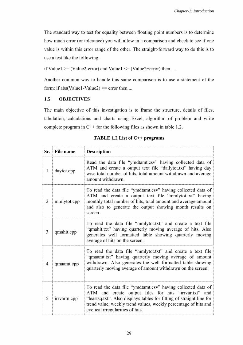
1.5 OBJECTIVES
The main objective of this investigation is to frame the structure, details of files,
tabulation, calculations and charts using Excel, algorithm of problem and write
complete program in C++ for the following files as shown in table 1.2.
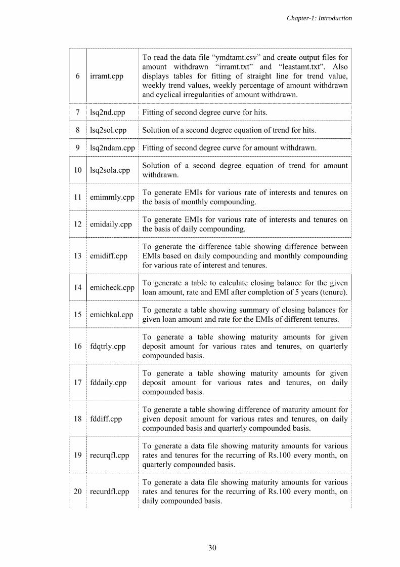
TABLE 1.2 List of C++ programs
Sr. File name Description
1 daytot.cpp
Read the data file “ymdtamt.csv” having collected data of ATM and create a output text file “dailytot.txt” having day wise total number of hits, total amount withdrawn and average amount withdrawn.
2 mmlytot.cpp
To read the data file “ymdtamt.csv” having collected data of ATM and create a output text file “mmlytot.txt” having monthly total number of hits, total amount and average amount and also to generate the output showing month results on screen.
3 qmahit.cpp
To read the data file “mmlytot.txt” and create a text file “qmahit.txt” having quarterly moving average of hits. Also generates well formatted table showing quarterly moving average of hits on the screen.
4 qmaamt.cpp
To read the data file “mmlytot.txt” and create a text file “qmaamt.txt” having quarterly moving average of amount withdrawn. Also generates the well formatted table showing quarterly moving average of amount withdrawn on the screen.
5 irrvartn.cpp
To read the data file “ymdtamt.csv” having collected data of ATM and create output files for hits “irrvar.txt” and “leastsq.txt”. Also displays tables for fitting of straight line for trend value, weekly trend values, weekly percentage of hits and cyclical irregularities of hits.
Chapter-1: Introduction
30
6 irramt.cpp
To read the data file “ymdtamt.csv” and create output files for amount withdrawn “irramt.txt” and “leastamt.txt”. Also displays tables for fitting of straight line for trend value, weekly trend values, weekly percentage of amount withdrawn and cyclical irregularities of amount withdrawn.
7 lsq2nd.cpp Fitting of second degree curve for hits.
8 lsq2sol.cpp Solution of a second degree equation of trend for hits.
9 lsq2ndam.cpp Fitting of second degree curve for amount withdrawn.
10 lsq2sola.cpp Solution of a second degree equation of trend for amount withdrawn.
11 emimmly.cpp To generate EMIs for various rate of interests and tenures on the basis of monthly compounding.
12 emidaily.cpp To generate EMIs for various rate of interests and tenures on the basis of daily compounding.
13 emidiff.cpp To generate the difference table showing difference between EMIs based on daily compounding and monthly compounding for various rate of interest and tenures.
14 emicheck.cpp To generate a table to calculate closing balance for the given loan amount, rate and EMI after completion of 5 years (tenure).
15 emichkal.cpp To generate a table showing summary of closing balances for given loan amount and rate for the EMIs of different tenures.
16 fdqtrly.cpp To generate a table showing maturity amounts for given deposit amount for various rates and tenures, on quarterly compounded basis.
17 fddaily.cpp To generate a table showing maturity amounts for given deposit amount for various rates and tenures, on daily compounded basis.
18 fddiff.cpp To generate a table showing difference of maturity amount for given deposit amount for various rates and tenures, on daily compounded basis and quarterly compounded basis.
19 recurqfl.cpp To generate a data file showing maturity amounts for various rates and tenures for the recurring of Rs.100 every month, on quarterly compounded basis.
20 recurdfl.cpp To generate a data file showing maturity amounts for various rates and tenures for the recurring of Rs.100 every month, on daily compounded basis.

Chapter-1: Introduction
31
21 recudiff.cpp
To generate a data file showing difference of maturity amounts for various rates and tenures for the recurring of Rs.100 every month, on daily compounded basis and quarterly compounded basis.
22 grfile.cpp To generate a data file for the calculation of initial solution of MLEs using graphical method - Weibull distribution for hits.
23 nrtable1.cpp To generate iterations of N-R method for the final solution of estimation of parameters - Weibull distribution for hits.
24 gramt.cpp To generate a data file for the calculation of initial solution of MLEs using graphical method - Weibull distribution for amount withdrawn per day.
25 nramt.cpp To generate iterations of N-R method for the final solution of estimation of parameters - Weibull distribution for amount withdrawn per day.
26 anovahit.cpp To generate ANOVA table for hits.
27 anovaamt.cpp To generate ANOVA table for amount withdrawn.
This will help the general public in finding
1. The EMI for the loan taken from the bank or any other financial institution.
2. The proper tenure for the loan using EMIs.
3. To find the amount calculated on the basis of daily and quarterly compounding
basis so that one can find how much the customer is loosing if the bank gives
interest on the basis of quarterly compounding instead of daily compounding.
Similarly for the amount taken from the bank.
So far such type of investigation for the bank or any financial institution has not been
made in past hence we took keen interest in such finding with the help of bank,
internet and website. The program developed in C++ in this investigation can be made
as software for the future plan.
From this investigation we concluded that how much amount a bank in the ATM can
deposit every day month wise or season wise so that customer will not return from the
ATM of the corresponding bank without taking required money. Which implies that
bank can be kept self in safety side by providing that much money in their ATM
based on mode in statistics.
Chapter-1: Introduction
32
To achieve these objectives, this thesis is structured as follows.
In chapter 1 we have covered general introduction regarding complete thesis. Mainly
we have covered following points in this chapter:
About Bank and Its Functions
Time Series Analysis
Weibull distribution
About C/C++ programming language
Chapter 2 describes the research methodology and data collection. We have collected
the ATM data from a bank located at Porbandar for the period of one year. In this
chapter we have described various aspects of data collection and handling like
structure of the collected data, data entry, data validations, and conversions of original
data into required format etc., also shown about the programming language C/C++.
Chapter 3 describes the time series analysis of hits and amount withdrawn from the
ATM. Here we have given general introduction of time series analysis. We have also
discussed various measurements of secular trends like freehand curve method, method
of moving averages, method of least squares and measurement of seasonal variations
like ratio to trend method. We have written C++ programs for these methods. We
have used Excel to draw various charts for these methods.
As we know that computers become more prevalent in everyday life, computer aided
office practice is fast becoming the avenue of choice for acquiring ease and accuracy
in day to day life. This will improve human facilities with the proper decision making
for the organization as well as people. Banking sector is one of the leading sectors,
where such office practice is very useful. The basic services a bank provides are
checking accounts, which can be used like money to make payments and purchase
goods and services; savings accounts and time deposits that can be used to save
money for future use; loans that consumers and businesses can use to purchase goods
and services; and basic cash management services such as check cashing and foreign
currency exchange. Banks are also called custodians of public money. Lending
money is one of the two major activities of any Bank. In a way, the Bank acts as an
intermediary between the people who have the money to lend and those who have the
need for money to carry out business transactions. Landing money to public is in form
Chapter-1: Introduction
33
of various types of loans like Housing loan, Personal loan, Education loan, Car loan
etc. In chapter 4 we have calculated EMIs for different rates of interest and different
tenures on the basis of monthly and daily compounding using C++. We have shown
the effect of rest basis by various difference tables.
Now one can earn a higher income on the surplus funds by investing those with bank.
The quantum of interest depends upon the rate of interest, term - length of time for
which the depositor wishes to keep the money with the Bank and method of
compounding. One can calculate maturity amount using different methods of
compounding. Here in chapter 5 we have calculated maturity amounts of various bank
deposits using method of quarterly compounding and method of daily compounding
using programs written in C++. We have shown the effect of rest basis by various
difference tables of maturity amounts.
As we have discussed in chapter 2 that we have collected ATM data for 1 year i.e. for
the period 01-01-2005 to 31-12-2005. Our main focus of the study is on number of
hits per day (number of customers visited to the ATM) and the amount withdrawn per
hit. In chapter 6 we have covered the fitting of Weibull distribution on hits and
amount withdrawn, we have applied method of maximum likelihood Estimation for
the estimation of parameters β and θ. Using C++ programs we have calculated initial
solution using graphical method. We have also generated all the iterations of N-R
method and found final solution using C++ program. We have also found the final
solution using goal seek method of Excel. We have calculated mean and variance
also. We have prepared the tables for goodness of fit test and found that hits and
amount withdrawn per day of a bank at Porbandar fits to the Weibull distribution.
Chapter-2: Research Methodology and Data Collection
34
Chapter
2 Research Methodology and Data Collection
2.1 DATA COLLECTION FROM BANK
In this age of global world, the ATM is good because it helps to solve problems for
which people don’t have time to stand in line waiting inside the bank or who do not
have patience of getting help from the tellers who are performing a slow job at the
window. It is also good for people who are travelling different places; they do not
need to carry their cash in their hands. It also gives you access to your saving account.
Thus ATMs are playing major role in customer services.
ATMs are providing many facilities, but we have focused our study only on
withdrawal of amount i.e. Study the number of customers visited per day and amount
withdrawn.
The most difficult task in achieving the objectives said was collection of data. The
data being confidential, it was quite essential to maintain the secrecy of the data as
well as the bank branch. I have visited so many banks, discussed with the concern
officers about our objectives and requested for the required data. I found it very
difficult to convince them due to their limitations. Ultimately I found one cooperative
and academic minded officer, who convinced with our objectives and permitted me to
collect the data from the bank.
Initially ATM machines are filled with blank paper roles, the details of each and every
transaction will be printed on the paper role, attached to the ATM. Printed paper roles
are dumped in the store room and replaced with the blank role 2-3 times in a month or
as and when necessary. We have focused only on the withdrawals and found date of
transaction, arrival time and amount withdrawal for each transaction i.e. each visit of
the customer.

Chapter-2: Research Methodology and Data Collection
35
That gentle, cooperative and academic minded officer has given me facility in the
branch to write these details.
We have noted down the data for about
365 days or 12 months or 17824 hits/ records/ withdrawals.
Considering our duty hours and bank pick hours, most of the data collection was done
after their regular timings only. All the transaction history was printed on a paper role
continuously; proper care was required to read each transaction without skipping any
transaction or duplication of transaction. It was a very lengthy and time consuming
process to write each and every transaction in the note book.
2.2 DATA PREPARATION IN EXCEL WORKSHEET
2.2.1 DATA ENTRY
Here we have selected Microsoft Excel worksheet for the data handling. We have
created three columns, each for date, time and amount withdrawn. Obviously the data
was ordered date wise and time wise chronologically. There are in total 17824 hits for
amount withdrawal so there are 17824 rows (records) and 3 columns in the worksheet.
2.2.2 DATA VALIDATION
As we are human being, there is a chance of incorrect entry. We have validated the
data, using facilities available in Excel, in following ways:
o Current time must not be less than the previous time, if date is same.
o Amount withdrawn per hit should not exceed the maximum limit. (Rs.40000.00)
o Amount should be positive.
Sample of the initial worksheet of the collected data is as under:

Chapter-2: Research Methodology and Data Collection
36
FIGURE 2.1
2.2.3 CONVERSION OF DATE AND TIME IN NUMERIC TYPE
We want some arithmetic process on date and time, so we have converted them into
numeric format.
Dates are converted as integer numbers. Considering 01-01-1900 as the first day, 01-
01-2005 is 38353rd day; 02-01-2005 is 38354th day and so on.
Considering one day as integer 1, each hour can become 24th part of 1 i.e. 0.041667.
For every one hour there will be in increment of 0.041667. Following table 2.1 shows
numeric conversion of hour.
TABLE 2.1
Time Format
NumberFormat
1:00 AM 0.0416672:00 AM 0.0833333:00 AM 0.1250004:00 AM 0.1666675:00 AM 0.2083336:00 AM 0.2500007:00 AM 0.2916678:00 AM 0.3333339:00 AM 0.375000
10:00 AM 0.41666711:00 AM 0.458333
12:00 NOON 0.5000001:00 PM 0.541667
2:00 PM 0.5833333:00 PM 0.6250004:00 PM 0.6666675:00 PM 0.7083336:00 PM 0.7500007:00 PM 0.7916678:00 PM 0.8333339:00 PM 0.875000
10:00 PM 0.91666711:00 PM 0.95833312:00 AM 1.000000
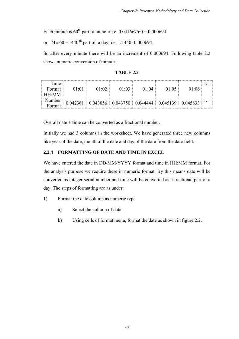
Chapter-2: Research Methodology and Data Collection
37
Each minute is 60th part of an hour i.e. 0.041667/60 = 0.000694
or 14406024 th part of a day, i.e. 1/1440=0.000694.
So after every minute there will be an increment of 0.000694. Following table 2.2
shows numeric conversion of minutes.
TABLE 2.2
Time Format
HH:MM 01:01 01:02 01:03 01:04 01:05 01:06
…
Number Format
0.042361 0.043056 0.043750 0.044444 0.045139 0.045833…
Overall date + time can be converted as a fractional number.
Initially we had 3 columns in the worksheet. We have generated three new columns
like year of the date, month of the date and day of the date from the date field.
2.2.4 FORMATTING OF DATE AND TIME IN EXCEL
We have entered the date in DD/MM/YYYY format and time in HH:MM format. For
the analysis purpose we require these in numeric format. By this means date will be
converted as integer serial number and time will be converted as a fractional part of a
day. The steps of formatting are as under:
1) Format the date column as numeric type
a) Select the column of date
b) Using cells of format menu, format the date as shown in figure 2.2.

Chapter-2: Research Methodology and Data Collection
38
FIGURE 2.2
2) Format the time column as numeric type
a) Select the column of time
b) Using cells of format menu, format the time as shown in figure 2.3.

Chapter-2: Research Methodology and Data Collection
39
FIGURE 2.3
3) Separate year, month and day of the date
a) Insert three columns B,C and D each for year, month and day
b) Get the year of the date by writing the formula =YEAR(E1) in B1
c) Get the month of the date by writing the formula =MONTH(E1) in C1
d) Get the day of the date by writing the formula =DAY(E1) in D1
e) Copy B1, C1 and D1 for all the dates
f) Finally we have created the worksheet ‘ymdtamt.xls’ file having
columns like Serial number, Numeric year of the date i.e. YEAR(E1),
Numeric month of the date i.e. MONTH(E1), Numeric day of the date

Chapter-2: Research Methodology and Data Collection
40
i.e. DAY(E1), Date as number format, Time as number format and
Amount.
Sample of the worksheet after conversion in above mentioned format is as under at
figure 2.4:
FIGURE 2.4
As we have used the C++ programming language, we require the data file accessible
through C++. To prepare the data file accessible to C++ we have saved the worksheet
in CSV format as under at figure 2.5:

Chapter-2: Research Methodology and Data Collection
41
FIGURE 2.5
Now, our data is ready for further processing. We have developed C++ programs to
read the data file ymdtamt.csv and generated various data files and results for the
different objectives.
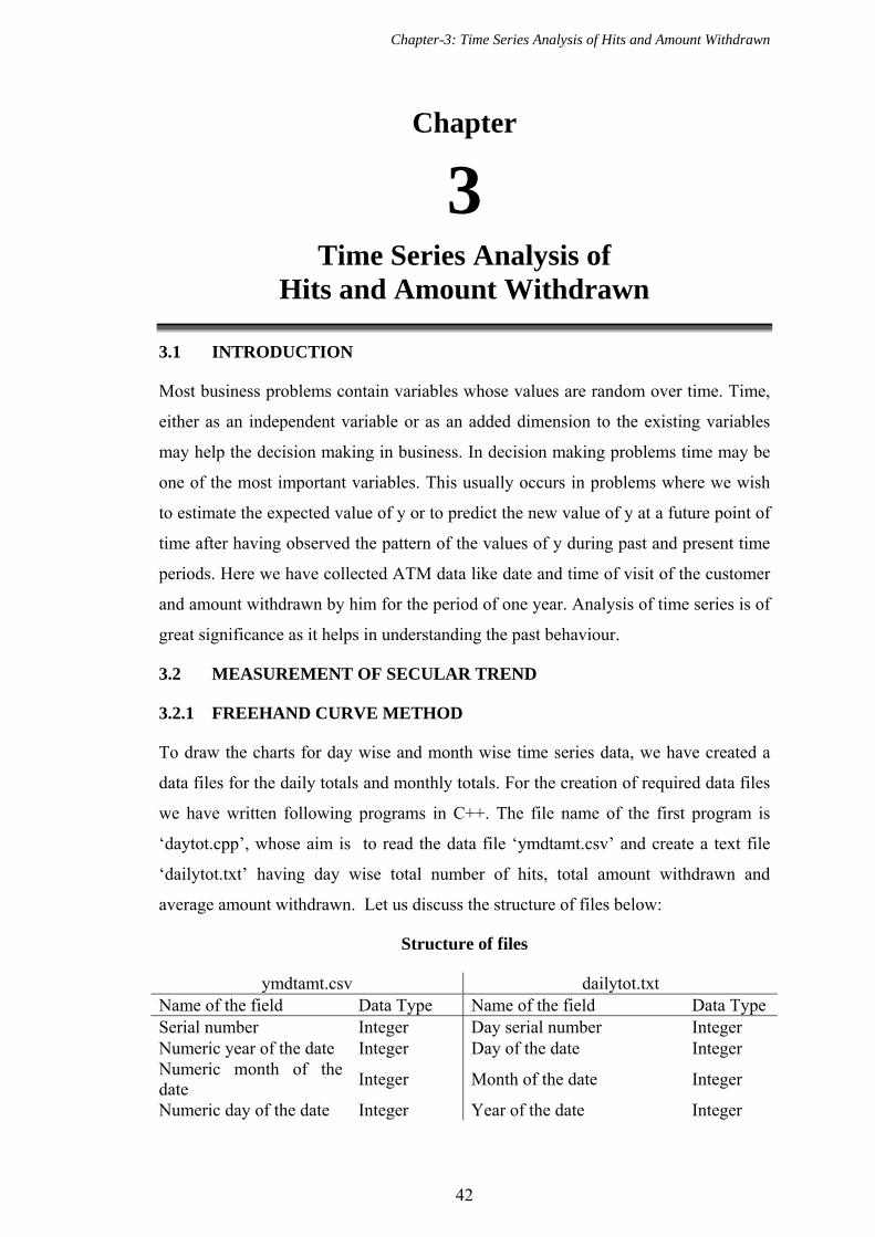
Chapter-3: Time Series Analysis of Hits and Amount Withdrawn
42
Chapter
3 Time Series Analysis of
Hits and Amount Withdrawn
3.1 INTRODUCTION
Most business problems contain variables whose values are random over time. Time,
either as an independent variable or as an added dimension to the existing variables
may help the decision making in business. In decision making problems time may be
one of the most important variables. This usually occurs in problems where we wish
to estimate the expected value of y or to predict the new value of y at a future point of
time after having observed the pattern of the values of y during past and present time
periods. Here we have collected ATM data like date and time of visit of the customer
and amount withdrawn by him for the period of one year. Analysis of time series is of
great significance as it helps in understanding the past behaviour.
3.2 MEASUREMENT OF SECULAR TREND
3.2.1 FREEHAND CURVE METHOD
To draw the charts for day wise and month wise time series data, we have created a
data files for the daily totals and monthly totals. For the creation of required data files
we have written following programs in C++. The file name of the first program is
‘daytot.cpp’, whose aim is to read the data file ‘ymdtamt.csv’ and create a text file
‘dailytot.txt’ having day wise total number of hits, total amount withdrawn and
average amount withdrawn. Let us discuss the structure of files below:
Structure of files
ymdtamt.csv dailytot.txt Name of the field Data Type Name of the field Data Type Serial number Integer Day serial number Integer Numeric year of the date Integer Day of the date Integer Numeric month of the date
Integer Month of the date Integer
Numeric day of the date Integer Year of the date Integer

Chapter-3: Time Series Analysis of Hits and Amount Withdrawn
43
Date as number format Long integer Total number of hits Integer Time as number format Double Total amount of withdrawal Double
Amount Double Average amount of withdrawal
Double
Here we cite a sample data for 15 days in the month of January 2005. The data are
shown in Table 3.1.
TABLE 3.1
Day serial
number
Day of the
date
Month of the
date
Year of the
date
Total number
of hits
Total amount of
withdrawal
Average amount of
withdrawal1 1 1 2005 41 129000 3146.342 2 1 2005 31 58500 1887.103 3 1 2005 36 115900 3219.444 4 1 2005 33 194700 5900.005 5 1 2005 30 127100 4236.676 6 1 2005 31 143100 4616.137 7 1 2005 27 98800 3659.268 8 1 2005 30 171200 5706.679 9 1 2005 23 75800 3295.65
10 10 1 2005 27 105200 3896.3011 11 1 2005 34 132000 3882.3512 12 1 2005 43 150600 3502.3313 13 1 2005 41 184300 4495.1214 14 1 2005 21 32700 1557.1415 15 1 2005 28 109700 3917.86
However we have collected the actual data for the period 01-01-2005 to 31-12-2005.
Initially for this program ‘daytot.cpp’, let the algorithm is given below:
1. Open an input data file1 “ymdtamt.csv” to read in “r” mode
2. Open an output data file2 “dailytot.txt” to write in “w” mode
3. Check for the end of the file in file1, if end of file then display appropriate
message and terminate the process.
4. If not end of file then set the counter 1 to serial number of day, dayno.
5. Read one by one record while not end of file and repeat following steps.
a. Set counters for total hits and total amount to zero.
b. Read one by one record and repeat following steps for the day of date is not
changed.
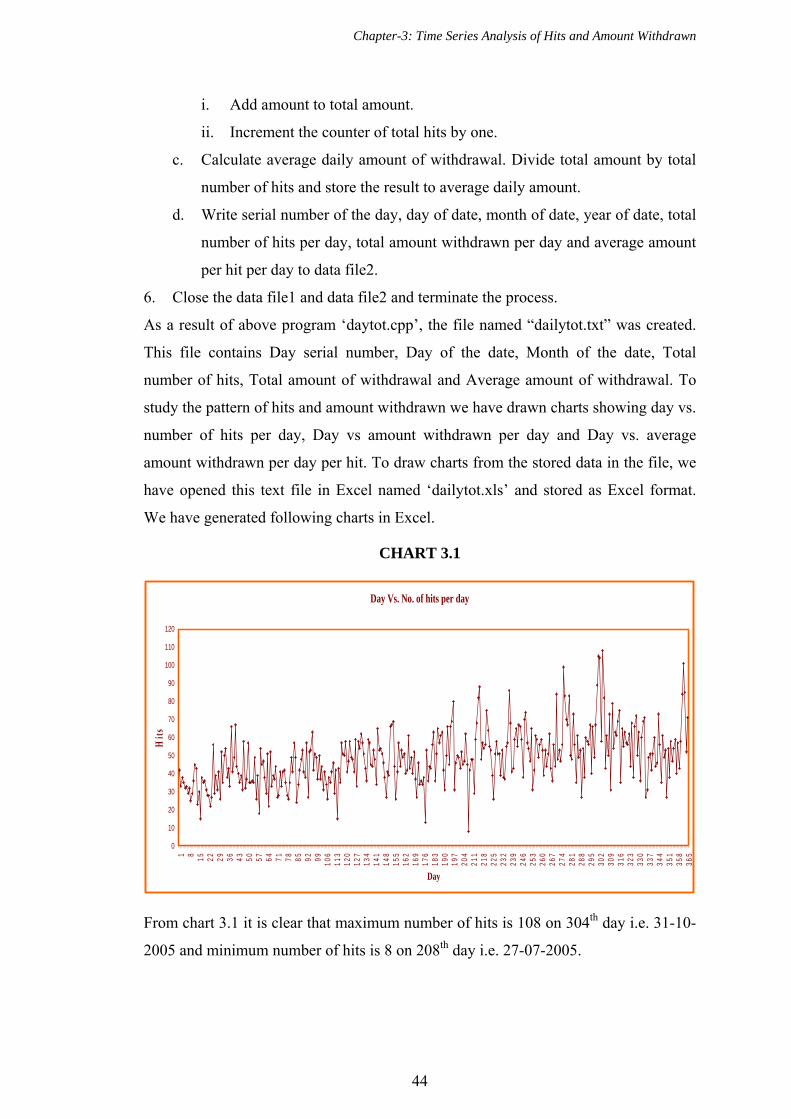
Chapter-3: Time Series Analysis of Hits and Amount Withdrawn
44
i. Add amount to total amount.
ii. Increment the counter of total hits by one.
c. Calculate average daily amount of withdrawal. Divide total amount by total
number of hits and store the result to average daily amount.
d. Write serial number of the day, day of date, month of date, year of date, total
number of hits per day, total amount withdrawn per day and average amount
per hit per day to data file2.
6. Close the data file1 and data file2 and terminate the process.
As a result of above program ‘daytot.cpp’, the file named “dailytot.txt” was created.
This file contains Day serial number, Day of the date, Month of the date, Total
number of hits, Total amount of withdrawal and Average amount of withdrawal. To
study the pattern of hits and amount withdrawn we have drawn charts showing day vs.
number of hits per day, Day vs amount withdrawn per day and Day vs. average
amount withdrawn per day per hit. To draw charts from the stored data in the file, we
have opened this text file in Excel named ‘dailytot.xls’ and stored as Excel format.
We have generated following charts in Excel.
CHART 3.1
Day Vs. No. of hits per day
0
10
20
30
40
50
60
70
80
90
100
110
120
1 81
52
22
93
64
35
05
76
47
17
88
59
29
910
611
312
012
713
414
114
815
516
216
917
618
319
019
720
421
121
822
523
223
924
625
326
026
727
428
128
829
530
230
931
632
333
033
734
435
135
836
5
Day
Hit
s
From chart 3.1 it is clear that maximum number of hits is 108 on 304th day i.e. 31-10-
2005 and minimum number of hits is 8 on 208th day i.e. 27-07-2005.

Chapter-3: Time Series Analysis of Hits and Amount Withdrawn
45
CHART 3.2
Day Vs. Amount withdrawn per day
0
100000
200000
300000
400000
500000
6000001 16 31 46 61 76 91 106
121
136
151
166
181
196
211
226
241
256
271
286
301
316
331
346
361
Day
Am
oun
t
From chart 3.2 it is clear that maximum amount withdrawn is Rs.523100 on 304th day
i.e. 31-10-2005 and minimum amount withdrawn is Rs.17000 on 16th day i.e. 16-01-
2005.
CHART 3.3
Day vs Average amount withdrawn per hit per day
0
1000
2000
3000
4000
5000
6000
7000
8000
1 16 31 46 61 76 91 106 121 136 151 166 181 196 211 226 241 256 271 286 301 316 331 346 361
Day
Ave
rage
From chart 3.3 it is clear that maximum average amount withdrawn is Rs.6920 on 80th
day i.e. 21-03-2005 and minimum average amount withdrawn is Rs.1133.33 on
16th day i.e. 16-01-2005.
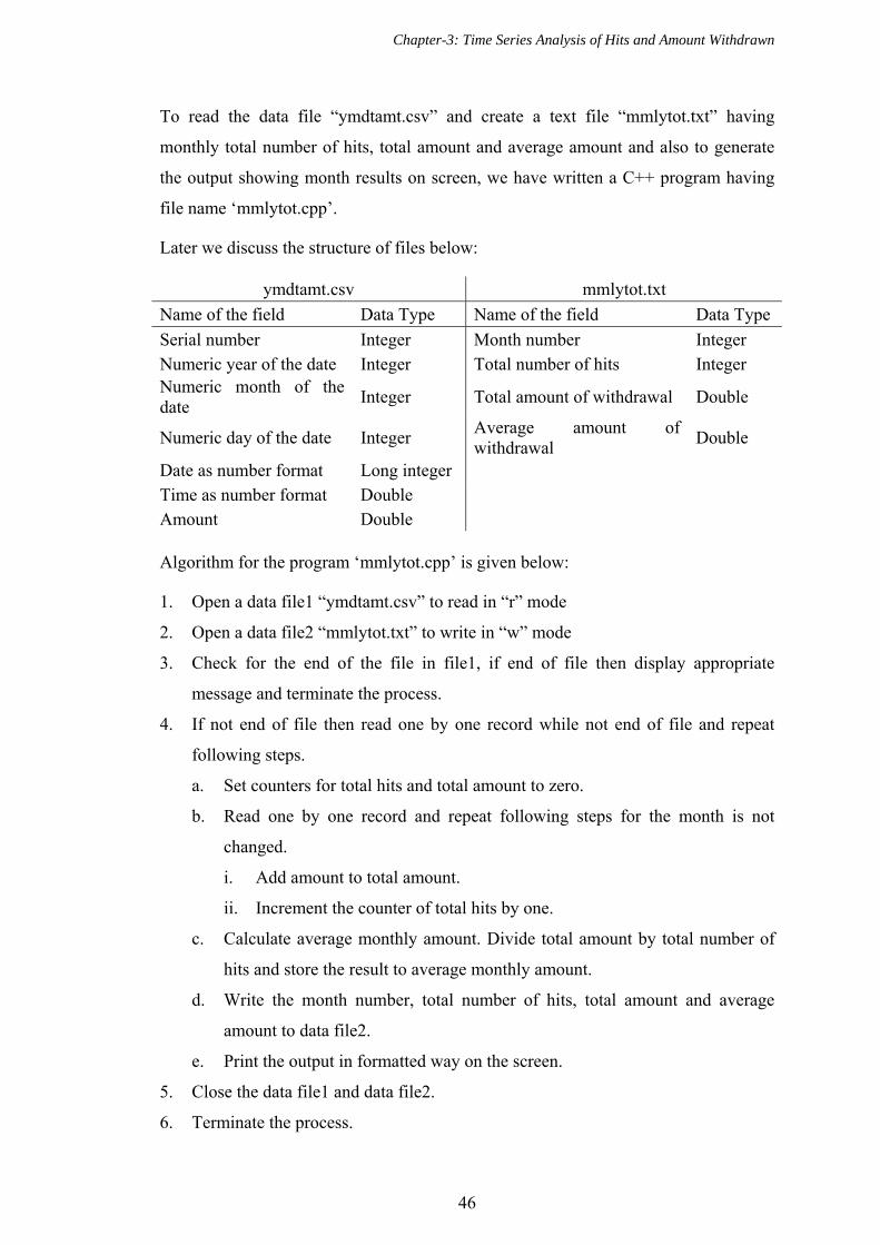
Chapter-3: Time Series Analysis of Hits and Amount Withdrawn
46
To read the data file “ymdtamt.csv” and create a text file “mmlytot.txt” having
monthly total number of hits, total amount and average amount and also to generate
the output showing month results on screen, we have written a C++ program having
file name ‘mmlytot.cpp’.
Later we discuss the structure of files below:
ymdtamt.csv mmlytot.txt
Name of the field Data Type Name of the field Data Type
Serial number Integer Month number Integer Numeric year of the date Integer Total number of hits Integer Numeric month of the date
Integer Total amount of withdrawal Double
Numeric day of the date Integer Average amount of withdrawal
Double
Date as number format Long integer Time as number format Double Amount Double Algorithm for the program ‘mmlytot.cpp’ is given below:
1. Open a data file1 “ymdtamt.csv” to read in “r” mode
2. Open a data file2 “mmlytot.txt” to write in “w” mode
3. Check for the end of the file in file1, if end of file then display appropriate
message and terminate the process.
4. If not end of file then read one by one record while not end of file and repeat
following steps.
a. Set counters for total hits and total amount to zero.
b. Read one by one record and repeat following steps for the month is not
changed.
i. Add amount to total amount.
ii. Increment the counter of total hits by one.
c. Calculate average monthly amount. Divide total amount by total number of
hits and store the result to average monthly amount.
d. Write the month number, total number of hits, total amount and average
amount to data file2.
e. Print the output in formatted way on the screen.
5. Close the data file1 and data file2.
6. Terminate the process.
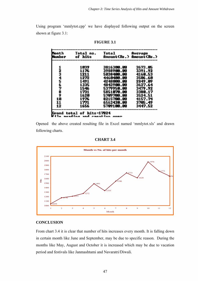
Chapter-3: Time Series Analysis of Hits and Amount Withdrawn
47
Using program ‘mmlytot.cpp’ we have displayed following output on the screen
shown at figure 3.1:
FIGURE 3.1
Opened the above created resulting file in Excel named ‘mmlytot.xls’ and drawn
following charts.
CHART 3.4
Month vs No. of hits per month
1039
11761211
1272
1491
1335
1546
1731
1620
1976
1771
1656
1000
1100
1200
1300
1400
1500
1600
1700
1800
1900
2000
2100
1 2 3 4 5 6 7 8 9 10 11 12
Month
Hits
CONCLUSION
From chart 3.4 it is clear that number of hits increases every month. It is falling down
in certain month like June and September, may be due to specific reason. During the
months like May, August and October it is increased which may be due to vacation
period and festivals like Janmashtami and Navaratri/Diwali.

Chapter-3: Time Series Analysis of Hits and Amount Withdrawn
48
CHART 3.5
Month vs Total amount withdrawn per month
38163003988900
5038400
44604004248000
4842900
5379950
58510705709700
8215700
6562430
5709100
3000000
3500000
4000000
4500000
5000000
5500000
6000000
6500000
7000000
7500000
8000000
8500000
1 2 3 4 5 6 7 8 9 10 11 12
Month
Am
ount
CONCLUSION
From chart 3.5 it is clear that month wise total amount withdrawn increases from 1st to
3rd month but from 4th and 5th month, it is decreasing due to specific reason. Again
from 5th month to 8th month, it increases in form of straight line. In the month of
October, it is increased very fast and again it decreases during 11th and 12th month.
CHART 3.6
Month vs Monthly average withdrawal per hit
3673.05
3391.92
4160.53
3506.60
2849.09
3627.64
3479.92
3380.17
3524.51
4157.74
3705.49
3447.52
2700.00
2800.00
2900.00
3000.00
3100.00
3200.00
3300.00
3400.00
3500.00
3600.00
3700.00
3800.00
3900.00
4000.00
4100.00
4200.00
4300.00
1 2 3 4 5 6 7 8 9 10 11 12
Month
Ave
rage
Chapter-3: Time Series Analysis of Hits and Amount Withdrawn
49
3.2.2 METHOD OF MOVING AVERAGES
We have already studied the trend through free hand method. These are very irregular
and having ups and down movements of the curves, so we need to study moving
average method.
The moving average series would yield a smooth curve. Here we have calculated
quarterly moving average using above created data file “mmlytot.txt”. This file
contains month wise total number of hits (total number of withdrawals per month),
total amount of withdrawal and average amount of withdrawal (i.e. total amount of
withdrawal / total number of hits).
To read the data file “mmlytot.txt” and create a text file “qmahit.txt” having quarterly
moving average of hits and also to generate the well formatted table showing
quarterly moving average of hits on the screen, we have prepared C++ programs
‘qmahit.cpp’ and ‘qmaamt.cpp’ for quarterly moving average of hits and quarterly
moving average of amount withdrawn respectively.
Structure of the output data file qmahit.txt is as under:
Name of the field Type-Format Month number Numeric- integer Quarterly moving average Numeric- float Algorithm for the program ‘qmahit.cpp’ is given below:
1. Open an input data file1 “mmlytot.txt” to read in “r” mode
2. Open an output data file2 “qmahit.txt” to write in “w” mode
3. Read the file “mmlytot.txt” up to end of file and generate two one dimensional
arrays to store month numbers and total number of hits per month. Thus we have
initialised two arrays namely mnth[] and hits[] with 12 elements each.
4. To calculate quarterly moving average for the months 2 to 11, repeat following
process for i= 2 to 11:
a. Calculate quarterly moving total, say mtot3[i], Calculate hits[i-1] + hits[i] +
hits[i+1] and store the result to mtot3[i].
b. Calculate quarterly moving average, say mavg3[i], calculate mtot3[i]/3 and
store the result to mavg3[i].

Chapter-3: Time Series Analysis of Hits and Amount Withdrawn
50
c. Write the month number and quarterly moving average to the output file
“qmahit.txt” and Print the month number, hits, quarterly moving total and
quarterly moving average in formatted way on the screen.
5. Close all data files and terminate the process.
Program ‘qmahit.cpp’ generates the table of quarterly moving average for month wise
number of hits and shows output on screen at figure 3.2:
FIGURE 3.2 Quarterly moving average for hits
We have opened the generated text file “qmahit.txt” in Excel, saved the same in Excel
format and generated following chart.
CHART 3.7
Quarterly moving average for hits
1142
1219
13241366
1457
1537
1632
1775 1789 1801
1000
1100
1200
1300
1400
1500
1600
1700
1800
1900
2 3 4 5 6 7 8 9 10 11
Month
Hits
CONCLUSION
From chart 3.7 it is clear that number of hits increases slowly 2nd month to 5th month,
but from 5th month to 9th month it increases rapidly. However 9th to 11th month,
number of hits is more or less same but it is in increasing sequence. Further we can
say that maximum number of hit is in 3rd and 4th quarter.

Chapter-3: Time Series Analysis of Hits and Amount Withdrawn
51
Similarly we have also created C++ program ‘qmaamt.cpp’ to generate the well
formatted table showing quarterly moving average of amount withdrawn.
FIGURE 3.3 Quarterly moving average for amount
We have also generated one output text file “qmaamt.txt” contains month number and
quarterly moving averages. We have opened this file in Excel and saved in Excel
format and generated following chart.
CHART 3.8
Quarterly Moving Average for Amount withdrawn
4281200
44959004582266.67
4517100
4823616.67
5357973.33
5646906.67
6592156.67
6829276.67 6829076.67
4000000
4250000
4500000
4750000
5000000
5250000
5500000
5750000
6000000
6250000
6500000
6750000
7000000
2 3 4 5 6 7 8 9 10 11
Month
Am
oun
t
CONCLUSION
From chart 3.8 it is clear that total amount withdrawn is more or less same from 1st
month to 5th month. However from 5th month, total amount withdrawn increase in the
form of straight line. This shows that from June to October people need to spend
much more money due to several personal and official purposes.
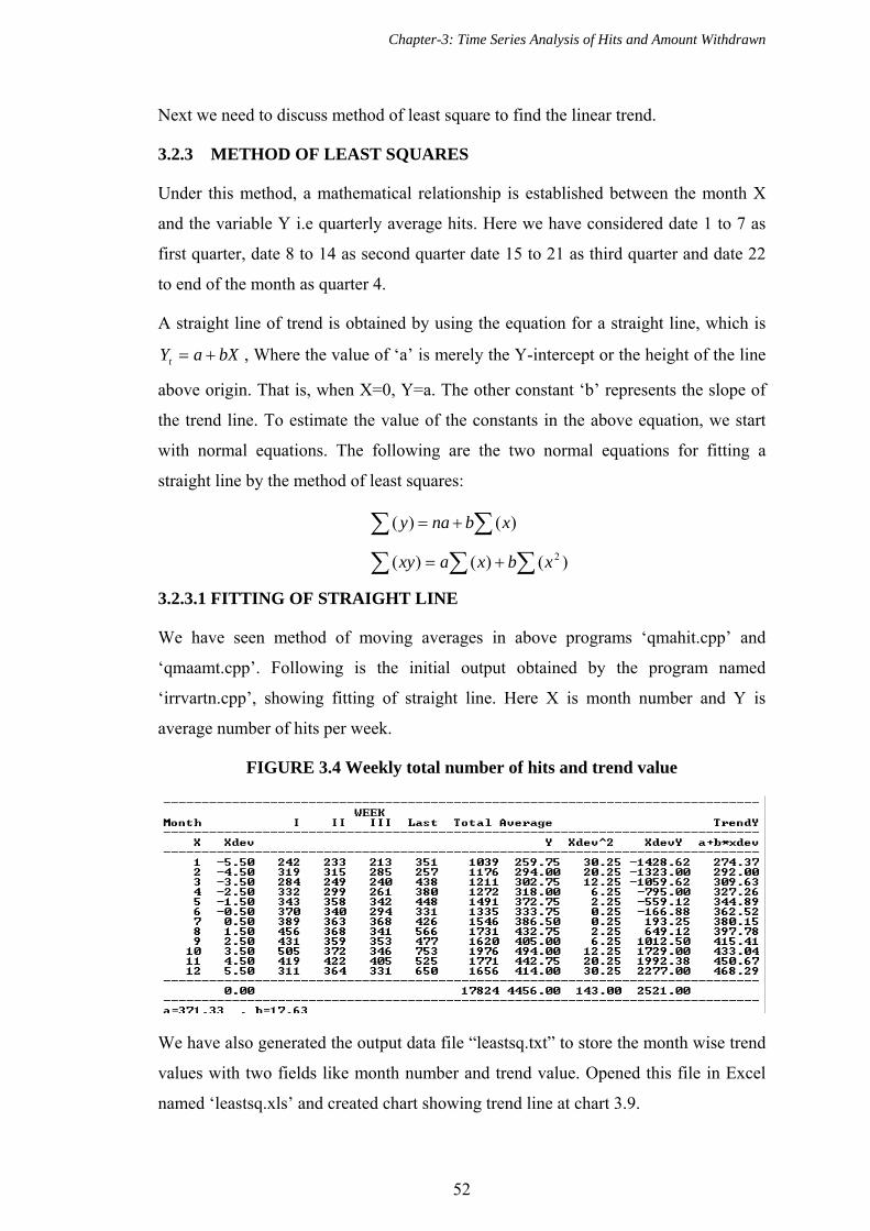
Chapter-3: Time Series Analysis of Hits and Amount Withdrawn
52
Next we need to discuss method of least square to find the linear trend.
3.2.3 METHOD OF LEAST SQUARES
Under this method, a mathematical relationship is established between the month X
and the variable Y i.e quarterly average hits. Here we have considered date 1 to 7 as
first quarter, date 8 to 14 as second quarter date 15 to 21 as third quarter and date 22
to end of the month as quarter 4.
A straight line of trend is obtained by using the equation for a straight line, which is
bXaYt , Where the value of ‘a’ is merely the Y-intercept or the height of the line
above origin. That is, when X=0, Y=a. The other constant ‘b’ represents the slope of
the trend line. To estimate the value of the constants in the above equation, we start
with normal equations. The following are the two normal equations for fitting a
straight line by the method of least squares:
)()( xbnay
)()()( 2xbxaxy
3.2.3.1 FITTING OF STRAIGHT LINE
We have seen method of moving averages in above programs ‘qmahit.cpp’ and
‘qmaamt.cpp’. Following is the initial output obtained by the program named
‘irrvartn.cpp’, showing fitting of straight line. Here X is month number and Y is
average number of hits per week.
FIGURE 3.4 Weekly total number of hits and trend value
We have also generated the output data file “leastsq.txt” to store the month wise trend
values with two fields like month number and trend value. Opened this file in Excel
named ‘leastsq.xls’ and created chart showing trend line at chart 3.9.

Chapter-3: Time Series Analysis of Hits and Amount Withdrawn
53
CHART 3.9
The line of best fit for hit
273.95
291.57
309.19
326.8
344.42
362.04
379.66
397.28
414.9
432.52
450.14
467.76
250
275
300
325
350
375
400
425
450
475
500
1 2 3 4 5 6 7 8 9 10 11 12
Month
Tre
nd
CONCLUSION
Here value of b is 17.63 i.e. positive, so the slope will be upwards. It is clearly seen
by the figures in the output and in chart, number of hits increases every month.
We have already studied least square method for average number of hits per week.
Similarly we have written the program ‘irramt.cpp’ and following is the initial output
obtained by the program named ‘irramt.cpp’, showing fitting of straight line. Here X
is month number and Y is average amount withdrawn per week.
FIGURE 3.5 Least square method for weekly total amount withdrawn

Chapter-3: Time Series Analysis of Hits and Amount Withdrawn
54
We have also generated the output data file “leastamt.txt” to store the month wise
trend values for amount withdrawn with two fields like month number and trend
value. Opened this file in Excel named ‘leastamt.xls’ and created following chart
showing trend line.
CHART 3.10
Line of best fit for amount
953835.94
1021657.62
1089479.38
1157301
1225122.75
1292944.38
1360766.12
1428587.75
1496409.5
1564231.12
1632052.88
1699874.62
800000
900000
1000000
1100000
1200000
1300000
1400000
1500000
1600000
1700000
1800000
1 2 3 4 5 6 7 8 9 10 11 12
Month
Tre
nd
Conclusion:
Here value of b is 67821.70 i.e. positive, so the slope will be upwards. It is clearly
seen by the figures in the output and in chart, Amount withdrawn per month increases
every month.
3.2.3.2 FITTING OF SECOND DEGREE CURVE
General form for second degree equation is 2cXbXaYt
2)()( xcxbnay
32 )()()( xcxbxaxy
4322 )()()( xcxbxayx
Following is the initial output obtained by the program named ‘lsq2nd.cpp’, showing
fitting of second degree curve for hits. Here X is month number and Y is average
number of hits per week.
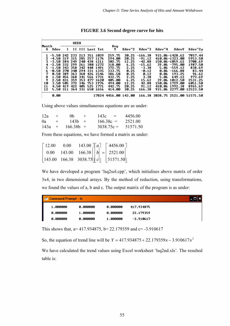
Chapter-3: Time Series Analysis of Hits and Amount Withdrawn
55
FIGURE 3.6 Second degree curve for hits
Using above values simultaneous equations are as under:
12a + 0b + 143c = 4456.00 0a + 143b + 166.38c = 2521.00 143a + 166.38b + 3038.75c = 51571.50
From these equations, we have formed a matrix as under:
50.51571
00.2521
00.4456
75.303838.16600.143
38.16600.14300.0
00.14300.000.12
c
b
a
We have developed a program ‘lsq2sol.cpp’, which initialises above matrix of order
3x4, in two dimensional arrays. By the method of reduction, using transformations,
we found the values of a, b and c. The output matrix of the program is as under:
This shows that, a= 417.934875, b= 22.179359 and c= -3.910617
So, the equation of trend line will be 2910617.3179359.22934875.417 xxY
We have calculated the trend values using Excel worksheet ‘lsq2nd.xls’. The resulted
table is:
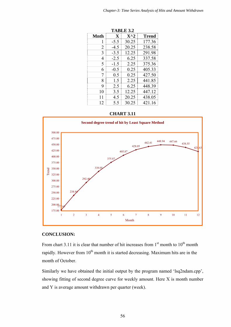
Chapter-3: Time Series Analysis of Hits and Amount Withdrawn
56
TABLE 3.2 Mnth X X^2 Trend
1 -5.5 30.25 177.362 -4.5 20.25 238.583 -3.5 12.25 291.984 -2.5 6.25 337.585 -1.5 2.25 375.366 -0.5 0.25 405.337 0.5 0.25 427.508 1.5 2.25 441.859 2.5 6.25 448.39
10 3.5 12.25 447.1211 4.5 20.25 438.0512 5.5 30.25 421.16
CHART 3.11
Second degree trend of hit by Least Square Method
177.65
238.94
292.40
338.05
375.87
405.87
428.05442.41 448.94 447.66
438.55
421.63
175.00
200.00
225.00
250.00
275.00
300.00
325.00
350.00
375.00
400.00
425.00
450.00
475.00
500.00
1 2 3 4 5 6 7 8 9 10 11 12
Month
Tre
nd
CONCLUSION:
From chart 3.11 it is clear that number of hit increases from 1st month to 10th month
rapidly. However from 10th month it is started decreasing. Maximum hits are in the
month of October.
Similarly we have obtained the initial output by the program named ‘lsq2ndam.cpp’,
showing fitting of second degree curve for weekly amount. Here X is month number
and Y is average amount withdrawn per quarter (week).
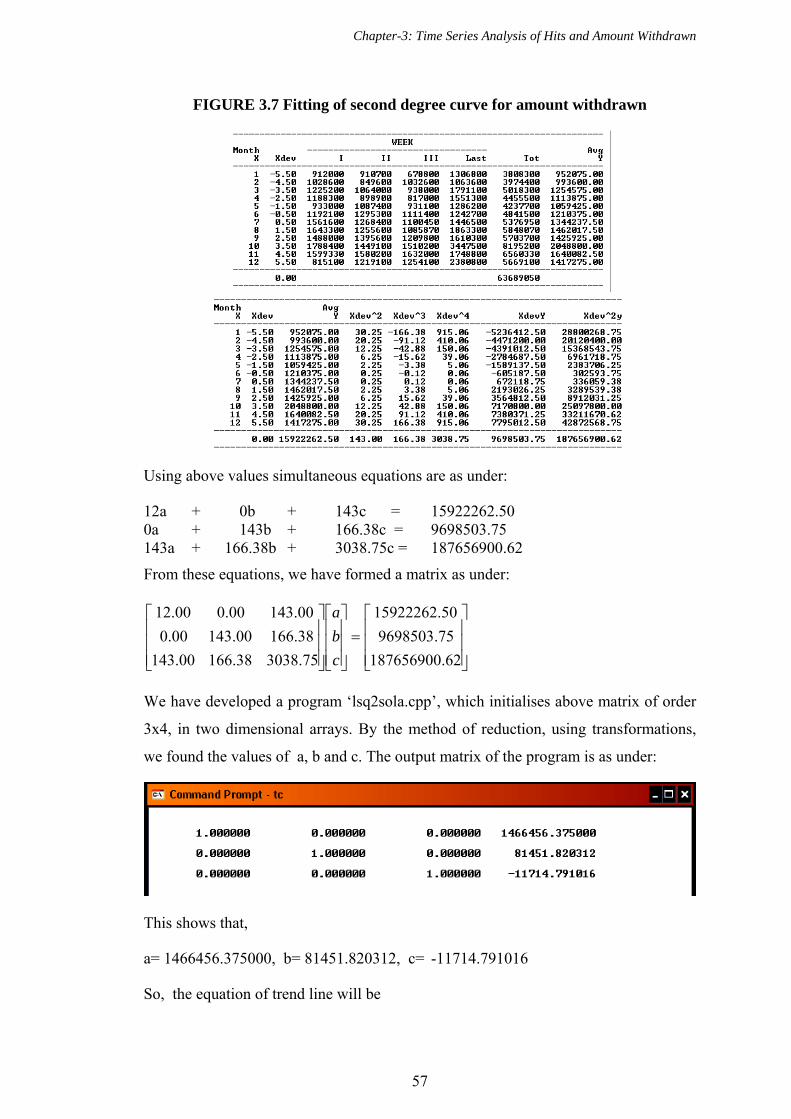
Chapter-3: Time Series Analysis of Hits and Amount Withdrawn
57
FIGURE 3.7 Fitting of second degree curve for amount withdrawn
Using above values simultaneous equations are as under:
12a + 0b + 143c = 15922262.50 0a + 143b + 166.38c = 9698503.75 143a + 166.38b + 3038.75c = 187656900.62
From these equations, we have formed a matrix as under:
62.187656900
75.9698503
50.15922262
75.303838.16600.143
38.16600.14300.0
00.14300.000.12
c
b
a
We have developed a program ‘lsq2sola.cpp’, which initialises above matrix of order
3x4, in two dimensional arrays. By the method of reduction, using transformations,
we found the values of a, b and c. The output matrix of the program is as under:
This shows that,
a= 1466456.375000, b= 81451.820312, c= -11714.791016
So, the equation of trend line will be

Chapter-3: Time Series Analysis of Hits and Amount Withdrawn
58
21611714.79101281451.820350001466456.37 xxY
We have calculated the trend values using Excel. The resulted table is as under:
TABLE 3.3
Month x x^2 Trend1 -5.5 30.25 664098.942 -4.5 20.25 862698.673 -3.5 12.25 1037868.814 -2.5 6.25 1189609.385 -1.5 2.25 1317920.366 -0.5 0.25 1422801.777 0.5 0.25 1504253.598 1.5 2.25 1562275.839 2.5 6.25 1596868.48
10 3.5 12.25 1608031.5611 4.5 20.25 1595765.0512 5.5 30.25 1560068.96
CHART 3.12
Second degree trend for amount withdrawn by Least Square Method
6640
98.94
8626
98.67
1037
868.8
1 1189
609.3
8 1317
920.3
614
2280
1.77
1504
253.5
9
1562
275.8
3
1596
868.4
8
1608
031.5
6
1595
765.0
5
1560
068.9
6
600000.00
800000.00
1000000.00
1200000.00
1400000.00
1600000.00
1800000.00
1 2 3 4 5 6 7 8 9 10 11 12
Month
Tre
nd
CONCLUSION
From chart 3.12 it is clear that amount withdrawn increases from 1st month to 10th
month rapidly. However from 10th month it is started decreasing. Maximum amount
withdrawn is in the month of October.
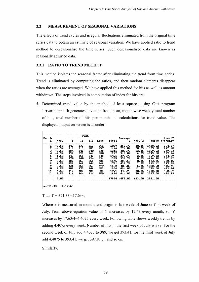
Chapter-3: Time Series Analysis of Hits and Amount Withdrawn
59
3.3 MEASUREMENT OF SEASONAL VARIATIONS
The effects of trend cycles and irregular fluctuations eliminated from the original time
series data to obtain an estimate of seasonal variation. We have applied ratio to trend
method to deseasonalise the time series. Such deseasonalised data are known as
seasonally adjusted data.
3.3.1 RATIO TO TREND METHOD
This method isolates the seasonal factor after eliminating the trend from time series.
Trend is eliminated by computing the ratios, and then random elements disappear
when the ratios are averaged. We have applied this method for hits as well as amount
withdrawn. The steps involved in computation of index for hits are:
5. Determined trend value by the method of least squares, using C++ program
‘irrvartn.cpp’. It generates deviation from mean, month wise weekly total number
of hits, total number of hits per month and calculations for trend value. The
displayed output on screen is as under:
Thus xY 63.1733.371 ,
Where x is measured in months and origin is last week of June or first week of
July. From above equation value of Y increases by 17.63 every month, so, Y
increases by 17.63/4=4.4075 every week. Following table shows weekly trends by
adding 4.4075 every week. Number of hits in the first week of July is 389. For the
second week of July add 4.4075 to 389, we get 393.41, for the third week of July
add 4.4075 to 393.41, we get 397.81 … and so on.
Similarly,

Chapter-3: Time Series Analysis of Hits and Amount Withdrawn
60
For the last week of June subtract 4.4075 from 389, we get 384.59, for the third
week of June subtract 4.4075 from 384.59, we get 380.19… and so on.
Thus we have generated table showing weekly trend values at figure 3.8.
FIGURE 3.8 Weekly trend values
6. Divide the original data quarter by quarter (Week as a quarter of the month) by the
corresponding trend values and express them as percentages. From above
mentioned outputs, in first week of January total number of hits=242, Weekly
trend = 283.22
10022.283
242Percentage =85.44 and so on for all respective values.
FIGURE 3.9 Weekly percentages of hits
7. Average the different values for a quarter.
8. Adjust all these averages and find the adjusted seasonal index, i.e. multiply each
average by 1200/1149.13.
It may be noted here that step (2) eliminates the trend and the values so obtained
include cyclical and irregular variations. Step (3) frees the values from cyclical and
irregular variations.

Chapter-3: Time Series Analysis of Hits and Amount Withdrawn
61
FIGURE 3.10 Cyclical irregularities
We have already studied measurement of seasonal variations for the visit of customer
to ATM i.e. number of hits. We have studied the same for the amount withdrawn also.
The steps involved in computation of index for amount withdrawn are:
1. Determined trend value by the method of least squares, using C++ program
‘irramt.cpp’. The received output is as shown in figure 3.11:
FIGURE 3.11 Weekly total amount withdrawn
Thus xY 70.6782125.1326855 ,
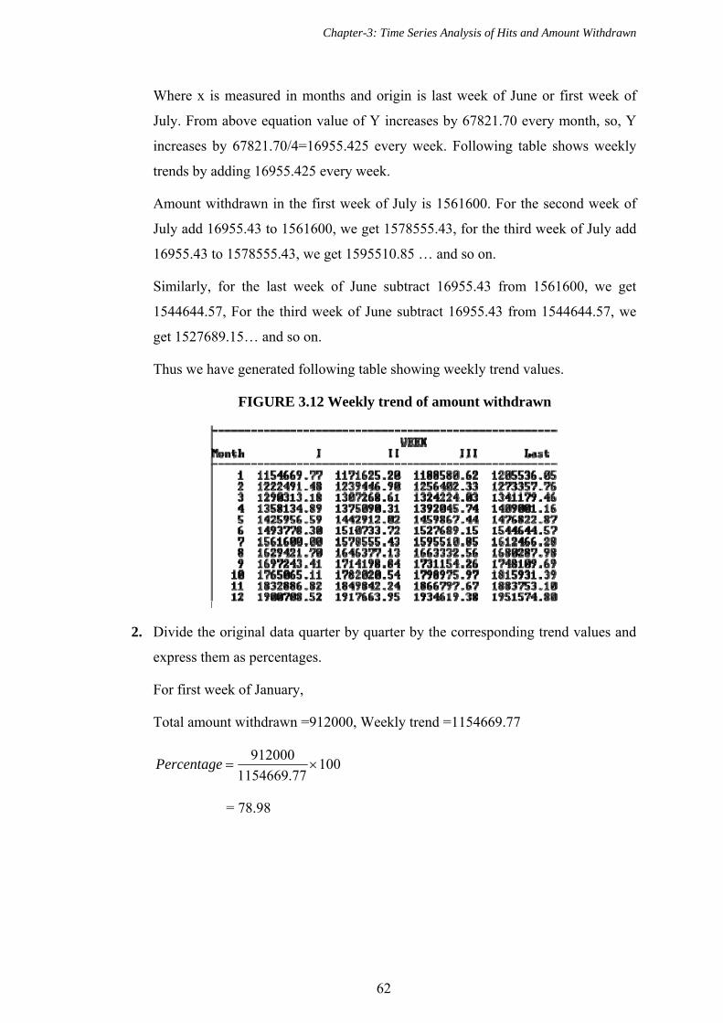
Chapter-3: Time Series Analysis of Hits and Amount Withdrawn
62
Where x is measured in months and origin is last week of June or first week of
July. From above equation value of Y increases by 67821.70 every month, so, Y
increases by 67821.70/4=16955.425 every week. Following table shows weekly
trends by adding 16955.425 every week.
Amount withdrawn in the first week of July is 1561600. For the second week of
July add 16955.43 to 1561600, we get 1578555.43, for the third week of July add
16955.43 to 1578555.43, we get 1595510.85 … and so on.
Similarly, for the last week of June subtract 16955.43 from 1561600, we get
1544644.57, For the third week of June subtract 16955.43 from 1544644.57, we
get 1527689.15… and so on.
Thus we have generated following table showing weekly trend values.
FIGURE 3.12 Weekly trend of amount withdrawn
2. Divide the original data quarter by quarter by the corresponding trend values and
express them as percentages.
For first week of January,
Total amount withdrawn =912000, Weekly trend =1154669.77
10077.1154669
912000Percentage
= 78.98
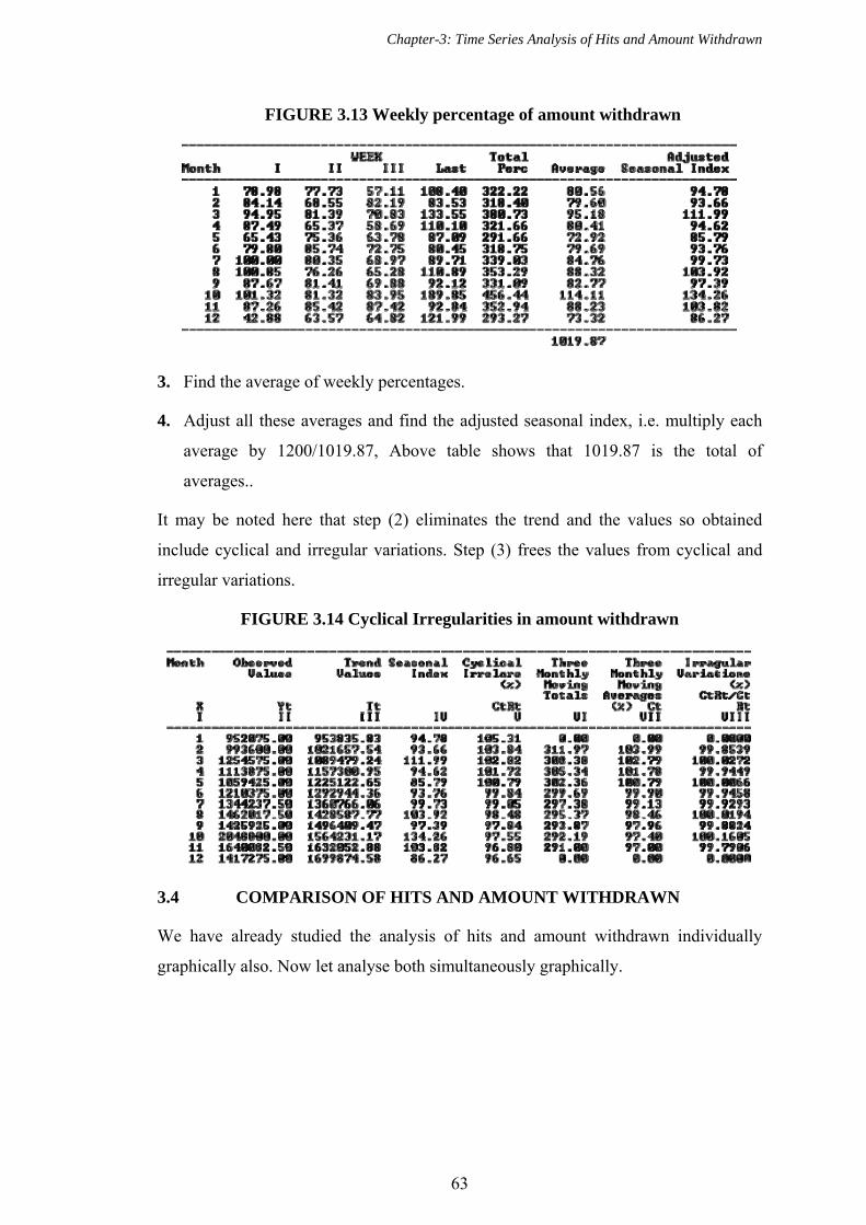
Chapter-3: Time Series Analysis of Hits and Amount Withdrawn
63
FIGURE 3.13 Weekly percentage of amount withdrawn
3. Find the average of weekly percentages.
4. Adjust all these averages and find the adjusted seasonal index, i.e. multiply each
average by 1200/1019.87, Above table shows that 1019.87 is the total of
averages..
It may be noted here that step (2) eliminates the trend and the values so obtained
include cyclical and irregular variations. Step (3) frees the values from cyclical and
irregular variations.
FIGURE 3.14 Cyclical Irregularities in amount withdrawn
3.4 COMPARISON OF HITS AND AMOUNT WITHDRAWN
We have already studied the analysis of hits and amount withdrawn individually
graphically also. Now let analyse both simultaneously graphically.

Chapter-3: Time Series Analysis of Hits and Amount Withdrawn
64
CHART 3.13 Day Vs. Number of hits and amount withdrawn for january
Day vs Number of hits and Amount withdrawn for January
0
5
10
15
20
25
30
35
40
45
50
55
601 2 3 4 5 6 7 8 9 10 11 12 13 14 15 16 17 18 19 20 21 22 23 24 25 26 27 28 29 30 31
Day
Hit
s
0
25000
50000
75000
100000
125000
150000
175000
200000
225000
250000
275000
Day
Am
oun
t
Amount Hits
From chart 3.13 it is seen that first two week and last two week the amount of
withdrawl is more compared to third week. This may be due to reason that in the
beginning and at the end money is required for marketing, tuition fees, electricity,
telephone bills etc. There is no perfect relation between number of hits and amount
withdrawn.

Chapter-3: Time Series Analysis of Hits and Amount Withdrawn
65
CHART 3.14 Month Vs. number of hits and amount withdrawn
Month vs Number of hits and Amount withdrawn
0
200
400
600
800
1000
1200
1400
1600
1800
2000
2200
1 2 3 4 5 6 7 8 9 10 11 12
Month
Hit
s
0
1000000
2000000
3000000
4000000
5000000
6000000
7000000
8000000
9000000
Month
Am
oun
t
Amount Hits
From chart 3.14 it is seen that amount withdrawn is more in the month of August,
October and November. This may be due to festival like Janmashtami, Navaratri and
new year where more money require for marketing. May is vacation time and hence
they go for tour and hence more money is also withdrawn in this month. In monthly
withdrawn it seems there is relation between number of hits and amount withdrawn as
number of hits increases amount withdrawn is also increases (except march and
April).

Chapter-3: Time Series Analysis of Hits and Amount Withdrawn
66
3.5 ANOVA FOR HITS
We have developed a C++ program named ‘anovahit.cpp’ to generate ANOVA table
for hits. The output of this program is shown here at figure 3.15.
FIGURE 3.15 Month wise weekly hits and sum of squares
Analysis of Variance (ANOVA) table
H0: Each week has same number of hits.
H1: Each week has different number of hits.
Conclusion: Here test is significant and hence H0 is rejected, that is, number of hits
per week are different.
**
*
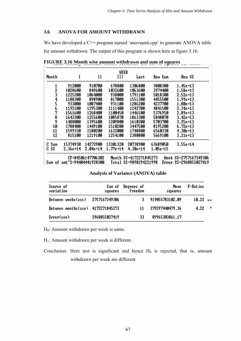
Chapter-3: Time Series Analysis of Hits and Amount Withdrawn
67
3.6 ANOVA FOR AMOUNT WITHDRAWN
We have developed a C++ program named ‘anovaamt.cpp’ to generate ANOVA table
for amount withdrawn. The output of this program is shown here at figure 3.16.
FIGURE 3.16 Month wise amount withdrawn and sum of squares
Analysis of Variance (ANOVA) table
H0: Amount withdrawn per week is same.
H1: Amount withdrawn per week is different.
Conclusion: Here test is significant and hence H0 is rejected, that is, amount
withdrawn per week are different.
**
*
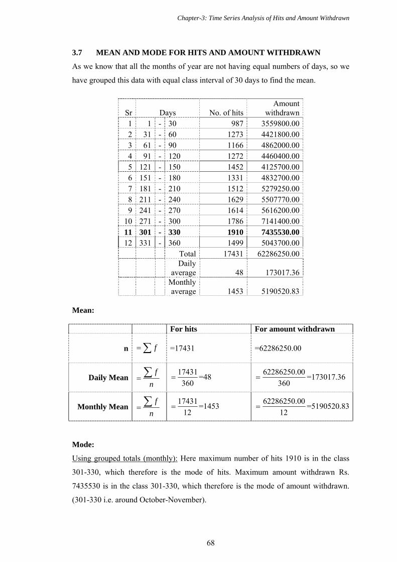
Chapter-3: Time Series Analysis of Hits and Amount Withdrawn
68
3.7 MEAN AND MODE FOR HITS AND AMOUNT WITHDRAWN
As we know that all the months of year are not having equal numbers of days, so we
have grouped this data with equal class interval of 30 days to find the mean.
Sr Days No. of hitsAmount
withdrawn 1 1 - 30 987 3559800.00 2 31 - 60 1273 4421800.00 3 61 - 90 1166 4862000.00 4 91 - 120 1272 4460400.00 5 121 - 150 1452 4125700.00 6 151 - 180 1331 4832700.00 7 181 - 210 1512 5279250.00 8 211 - 240 1629 5507770.00 9 241 - 270 1614 5616200.00
10 271 - 300 1786 7141400.00 11 301 - 330 1910 7435530.00 12 331 - 360 1499 5043700.00
Total 17431 62286250.00
Daily
average 48 173017.36
Monthly average 1453 5190520.83
Mean:
For hits For amount withdrawn
n f =17431 =62286250.00
Daily Mean n
f 360
17431 =48
360
062286250.0 =173017.36
Monthly Mean n
f 12
17431 =1453
12
062286250.0 =5190520.83
Mode:
Using grouped totals (monthly): Here maximum number of hits 1910 is in the class
301-330, which therefore is the mode of hits. Maximum amount withdrawn Rs.
7435530 is in the class 301-330, which therefore is the mode of amount withdrawn.
(301-330 i.e. around October-November).

Chapter-3: Time Series Analysis of Hits and Amount Withdrawn
69
Using daily totals: Here maximum number of hits per day is 108 on 31-10-2005,
which is therefore is the mode of hits and maximum amount withdrawn Rs.523100 is
also on 31-10-2005, which therefore is the mode of amount withdrawn per day.
HitsAmount
withdrawnTotal 17824 63822850
Maximum 108 523100
This shows that bank must keep amount of Rs. 523100 per day and Rs. 7435530 per
month. Again from chart 3.11 and 3.12 it is clear that number of hits and amount
withdrawn increase from 1st month to 10th month rapidly. However from 10th month it
is started decreasing. Maximum hits and amount withdrawn are in the month of
October.
If it is considered then it assured that customer will not return without collecting
money from the ATM. If money is kept less than those values then some customers
will return without taking money.
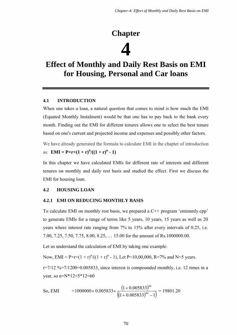
Chapter-4: Effect of Monthly and Daily Rest Basis on EMI
70
Chapter
4 Effect of Monthly and Daily Rest Basis on EMI
for Housing, Personal and Car loans
4.1 INTRODUCTION
When one takes a loan, a natural question that comes to mind is how much the EMI
(Equated Monthly Instalment) would be that one has to pay back to the bank every
month. Finding out the EMI for different tenures allows one to select the best tenure
based on one's current and projected income and expenses and possibly other factors.
We have already generated the formula to calculate EMI in the chapter of introduction
as: EMI = P×r×(1 + r)n/((1 + r)n - 1)
In this chapter we have calculated EMIs for different rate of interests and different
tenures on monthly and daily rest basis and studied the effect. First we discuss the
EMI for housing loan.
4.2 HOUSING LOAN
4.2.1 EMI ON REDUCING MONTHLY BASIS
To calculate EMI on monthly rest basis, we prepared a C++ program ‘emimmly.cpp’
to generate EMIs for a range of terms like 5 years, 10 years, 15 years as well as 20
years where interest rate ranging from 7% to 15% after every intervals of 0.25, i.e.
7.00, 7.25, 7.50, 7.75, 8.00, 8.25, … 15.00 for the amount of Rs.1000000.00.
Let us understand the calculation of EMI by taking one example:
Now, EMI = P×r×(1 + r)n/((1 + r)n - 1), Let P=10,00,000, R=7% and N=5 years.
r=7/12 %=7/1200=0.005833, since interest is compounded monthly, i.e. 12 times in a
year, so n=N*12=5*12=60
So, EMI =
1005833.01
005833.01005833.01000000
60
60
= 19801.20
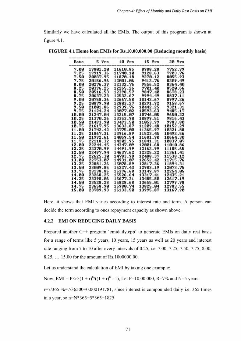
Chapter-4: Effect of Monthly and Daily Rest Basis on EMI
71
Similarly we have calculated all the EMIs. The output of this program is shown at
figure 4.1.
FIGURE 4.1 Home loan EMIs for Rs.10,00,000.00 (Reducing monthly basis)
Here, it shows that EMI varies according to interest rate and term. A person can
decide the term according to ones repayment capacity as shown above.
4.2.2 EMI ON REDUCING DAILY BASIS
Prepared another C++ program ‘emidaily.cpp’ to generate EMIs on daily rest basis
for a range of terms like 5 years, 10 years, 15 years as well as 20 years and interest
rate ranging from 7 to 10 after every intervals of 0.25, i.e. 7.00, 7.25, 7.50, 7.75, 8.00,
8.25, … 15.00 for the amount of Rs.1000000.00.
Let us understand the calculation of EMI by taking one example:
Now, EMI = P×r×(1 + r)n/((1 + r)n - 1), Let P=10,00,000, R=7% and N=5 years.
r=7/365 %=7/36500=0.000191781, since interest is compounded daily i.e. 365 times
in a year, so n=N*365=5*365=1825

Chapter-4: Effect of Monthly and Daily Rest Basis on EMI
72
So, EMI for a day =
110.000191781
10.00019178110.000191781000000
1825
1825
= 649.4698
So, EMI for a month = 649.4698 * (365/12) = 19754.71
Similarly we have calculated all the EMIs. The output of this program is at figure 4.2.
FIGURE 4.2 Home loan EMIs for Rs.10,00,000.00 (reducing daily basis)
Here, both figure 4.1 and figure 4.2 clearly indicates that amount of EMI with
reducing daily rest basis is less than the EMI with reducing monthly rest basis.
4.2.3 DIFFERENCE OF EMI ON REDUCING MONTHLY AND DAILY
BASIS
To see the clear difference of EMI amount for daily and monthly reducing basis,
prepared a C++ program ‘emidiff.cpp’. The output is at figure 4.3.

Chapter-4: Effect of Monthly and Daily Rest Basis on EMI
73
FIGURE 4.3
From figure 4.3 we conclude that daily reducing basis is less EMI than monthly
reducing basis. For the tenure of 5 years the difference of EMI is ranging from
Rs.2790 to Rs.5758, for the tenure of 10 years the difference of EMI is ranging from
2706 to 5023, for the tenure of 15 years the difference of EMI is ranging from 2573 to
4032 and for the tenure of 20 years the difference of EMI is ranging from 2401 to
3006 on monthly repayment of the loan.
We draw the chart for Rate of interest Vs. yearwise EMI difference and shown at
chart number 4.1.
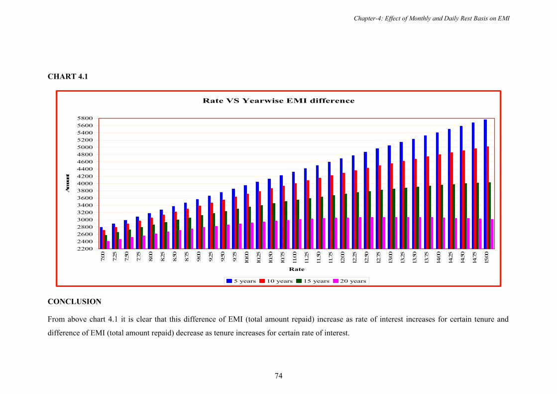
Chapter-4: Effect of Monthly and Daily Rest Basis on EMI
74
CHART 4.1
Rate VS Yearwise EMI difference
2200
2400
2600
2800
3000
3200
3400
3600
3800
4000
4200
4400
4600
4800
5000
5200
5400
5600
5800
7.00
7.25
7.50
7.75
8.00
8.25
8.50
8.75
9.00
9.25
9.50
9.75
10.00
10.25
10.50
10.75
11.00
11.25
11.50
11.75
12.00
12.25
12.50
12.75
13.00
13.25
13.50
13.75
14.00
14.25
14.50
14.75
15.00
Rate
Am
ount
5 years 10 years 15 years 20 years
CONCLUSION
From above chart 4.1 it is clear that this difference of EMI (total amount repaid) increase as rate of interest increases for certain tenure and
difference of EMI (total amount repaid) decrease as tenure increases for certain rate of interest.

Chapter-4: Effect of Monthly and Daily Rest Basis on EMI
75
4.2.4 RATE OF INTEREST AND EMI OF VARIOUS BANKS FOR
DIFFERENT PERIODS
For the academic interest, we have collected home loan interest rates and EMI
amount (As on 01-03-2010) of various banks from the web site ecompare.co.in. We
have also visited banks of surrounding area to verify the rates and EMIs. As our
interest is only to know the amount of EMI at certain rate of interest and certain
tenure, the lender bank and the effective date is not important for us. Following tables
show interest rates and EMI of various banks for different tenure like 5 years, 10
years, 15 years and 20 years. That will be useful to compare our program generated
EMIs:
TABLE 4.1 Compilation of Resident Home Loan Search Results for Rs. 10,00,000 Updated on 01 March 2010
5 years 10 years 15 years 20 years
Financial Institution Rate EMI Rate EMI Rate EMI Rate EMI
Dena Bank 9.75 21124 10.25 13354 10.25 10900 10.25 9816
Punjab & Sind Bank 9.00 20758 11 13775 11 11366 11.00 10322
Federal Bank 10.00 21494 11 13775 11 11366 11.00 10322
Allahabad bank 9.25 20880 9.25 12803 9.25 10292 9.25 9159
Indian Bank 10.50 21494 11 13775
United Bank 8.75 20637 8.75 12533
Bank of Baroda 9.50 21002 9.75 13077 10.00 10746
Syndicate Bank 10.75 21618 11.75 14203
Punjab National Bank 9.25 20880 10.00 13215 10.50 11054 10.50 9984
Indian Overses Bank 9.00 20758 9.50 12940
UCO Bank 11.75 22118 11.75 14203 12.00 12002 12.00 11011
Bank of India
Corporation Bank 11.00 21742 11 13775 11 11366 11 10322
Union Bank of India 9.50 21002
IDBI Bank 11.25 21867
Central Bank of India 10.00 21247
Vijaya Bank 10.75 21618
State Bank of India 10.75 21618 10.75 13634
Canara Bank
J & K Bank 10.25 21370 11 13775
Andhra Bank
Karur Vysya Bank 12.00 22244 12.50 14638 13.00 12652
South indian Bank 12.50 22498 13.5 15227 12.75 12488 12.75 11538
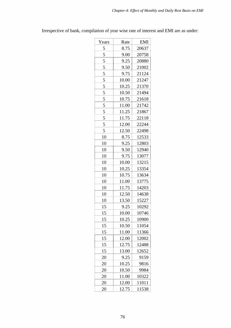
Chapter-4: Effect of Monthly and Daily Rest Basis on EMI
76
Irrespective of bank, compilation of year wise rate of interest and EMI are as under:
Years Rate EMI5 8.75 206375 9.00 207585 9.25 208805 9.50 210025 9.75 211245 10.00 212475 10.25 213705 10.50 214945 10.75 216185 11.00 217425 11.25 218675 11.75 221185 12.00 222445 12.50 2249810 8.75 1253310 9.25 1280310 9.50 1294010 9.75 1307710 10.00 1321510 10.25 1335410 10.75 1363410 11.00 1377510 11.75 1420310 12.50 1463810 13.50 1522715 9.25 1029215 10.00 1074615 10.25 1090015 10.50 1105415 11.00 1136615 12.00 1200215 12.75 1248815 13.00 1265220 9.25 915920 10.25 981620 10.50 998420 11.00 1032220 12.00 1101120 12.75 11538
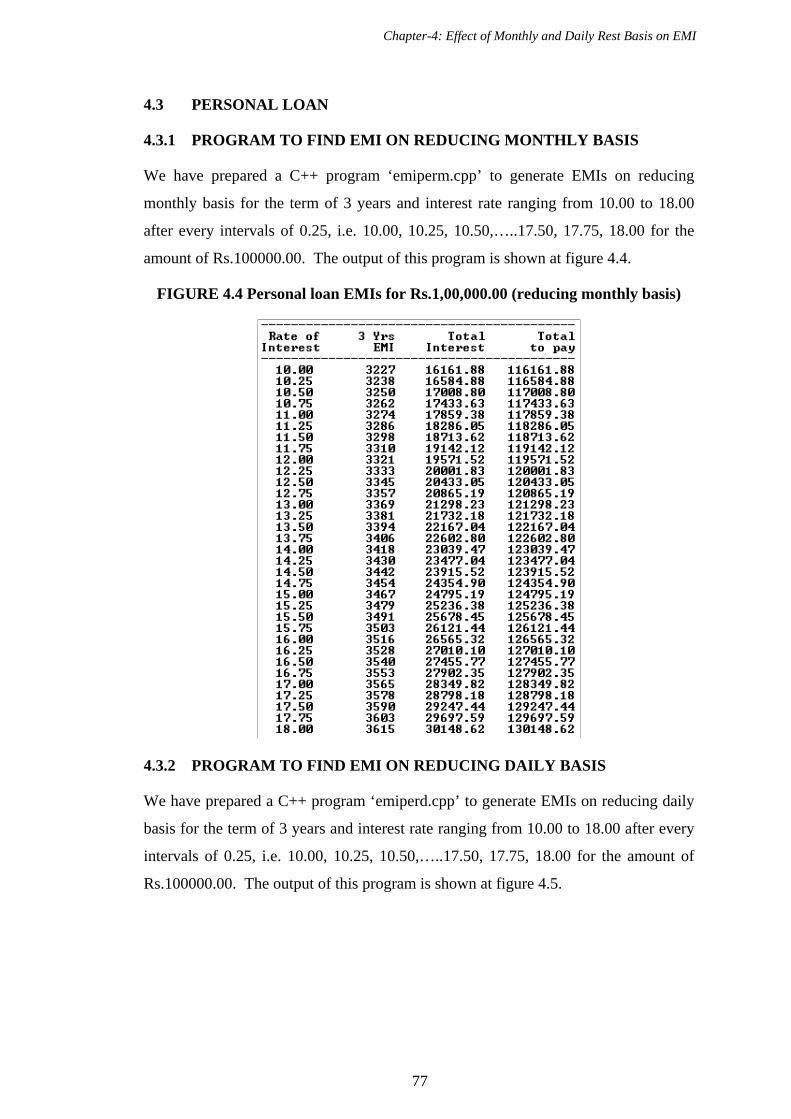
Chapter-4: Effect of Monthly and Daily Rest Basis on EMI
77
4.3 PERSONAL LOAN
4.3.1 PROGRAM TO FIND EMI ON REDUCING MONTHLY BASIS
We have prepared a C++ program ‘emiperm.cpp’ to generate EMIs on reducing
monthly basis for the term of 3 years and interest rate ranging from 10.00 to 18.00
after every intervals of 0.25, i.e. 10.00, 10.25, 10.50,…..17.50, 17.75, 18.00 for the
amount of Rs.100000.00. The output of this program is shown at figure 4.4.
FIGURE 4.4 Personal loan EMIs for Rs.1,00,000.00 (reducing monthly basis)
4.3.2 PROGRAM TO FIND EMI ON REDUCING DAILY BASIS
We have prepared a C++ program ‘emiperd.cpp’ to generate EMIs on reducing daily
basis for the term of 3 years and interest rate ranging from 10.00 to 18.00 after every
intervals of 0.25, i.e. 10.00, 10.25, 10.50,…..17.50, 17.75, 18.00 for the amount of
Rs.100000.00. The output of this program is shown at figure 4.5.
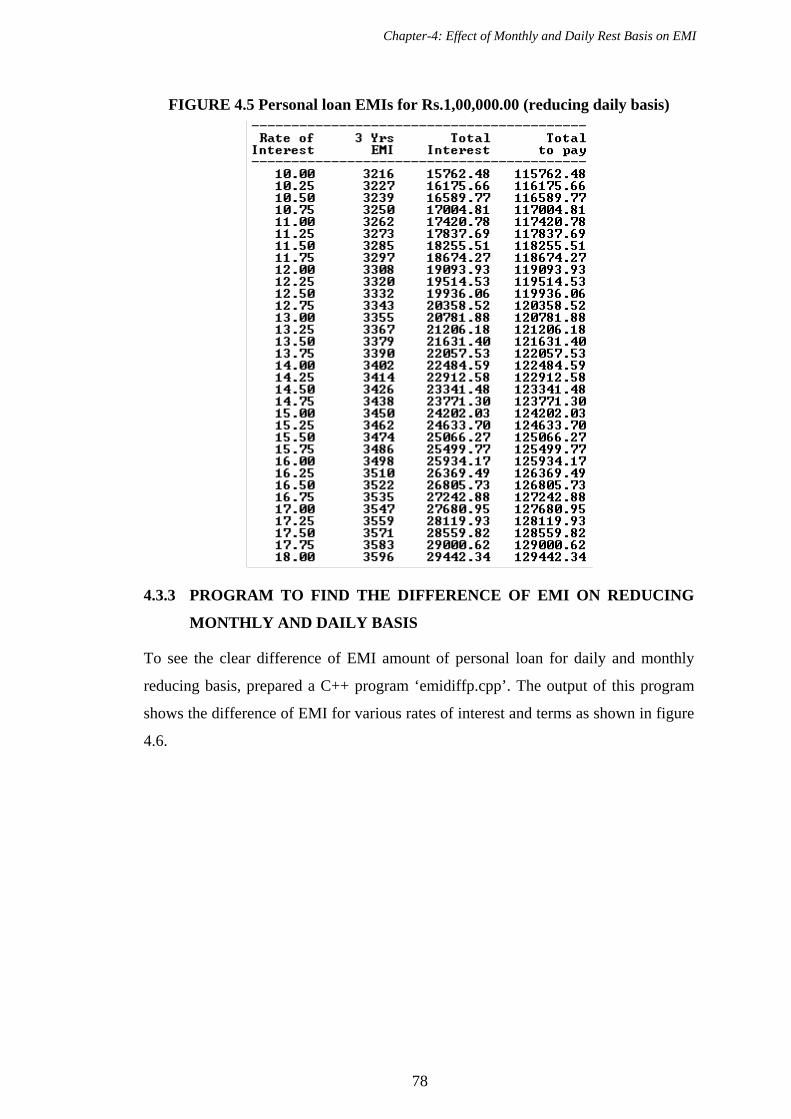
Chapter-4: Effect of Monthly and Daily Rest Basis on EMI
78
FIGURE 4.5 Personal loan EMIs for Rs.1,00,000.00 (reducing daily basis)
4.3.3 PROGRAM TO FIND THE DIFFERENCE OF EMI ON REDUCING
MONTHLY AND DAILY BASIS
To see the clear difference of EMI amount of personal loan for daily and monthly
reducing basis, prepared a C++ program ‘emidiffp.cpp’. The output of this program
shows the difference of EMI for various rates of interest and terms as shown in figure
4.6.
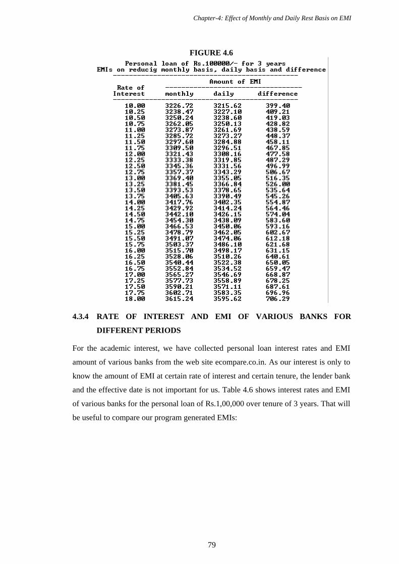
Chapter-4: Effect of Monthly and Daily Rest Basis on EMI
79
FIGURE 4.6
4.3.4 RATE OF INTEREST AND EMI OF VARIOUS BANKS FOR
DIFFERENT PERIODS
For the academic interest, we have collected personal loan interest rates and EMI
amount of various banks from the web site ecompare.co.in. As our interest is only to
know the amount of EMI at certain rate of interest and certain tenure, the lender bank
and the effective date is not important for us. Table 4.6 shows interest rates and EMI
of various banks for the personal loan of Rs.1,00,000 over tenure of 3 years. That will
be useful to compare our program generated EMIs:

Chapter-4: Effect of Monthly and Daily Rest Basis on EMI
80
TABLE 4.2 Personal Loan Search Results for 1,00,000 over 3 years
Updated on 01 March 2010
Sr. No.
Financial Institution
InterestRate
EMITotal
Interest Total
To Pay
1 Bank of India 11.50% 3298 18714 118714
2 Union Bank of India 11.75% 3310 19142 119142
3 United Bank 12.75% 3357 20865 120865
4 Central Bank of India 13.00% 3369 21298 121298
5 Allahabad Bank 13.00% 3369 21298 121298
6 Oriental Bank 13.00% 3369 21298 121298
7 Vijaya Bank 13.25% 3381 21732 121732
8 UCO Bank 13.25% 3381 21732 121732
9 Canara Bank 13.75% 3406 22603 122603
10 Indian Bank 13.75% 3406 22603 122603
11 Punjab & Sind Bank 14.00% 3418 23039 123039
12 Bank of Maharashtra 14.25% 3430 23477 123477
13 Corporation Bank 14.50% 3442 23916 123916
14 Dena Bank 15.00% 3467 24795 124795
15 South Indian Bank 15.25% 3479 25236 125236
16 Bank of Baroda 15.25% 3479 25236 125236
17 Karur Vysya Bank 15.50% 3491 25678 125678
18 State Bank of India 16.00% 3516 26565 126565
19 Federal Bank 16.25% 3528 27010 127010
20 IndusInd Bank 17.00% 3565 28350 128350
21 ABN-AMRO 17.75% 3603 29698 129698
22 Kotak 19.00% 3666 31962 131962
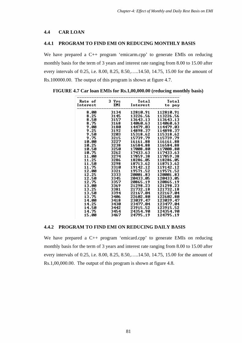
Chapter-4: Effect of Monthly and Daily Rest Basis on EMI
81
4.4 CAR LOAN 4.4.1 PROGRAM TO FIND EMI ON REDUCING MONTHLY BASIS We have prepared a C++ program ‘emicarm.cpp’ to generate EMIs on reducing
monthly basis for the term of 3 years and interest rate ranging from 8.00 to 15.00 after
every intervals of 0.25, i.e. 8.00, 8.25, 8.50,…..14.50, 14.75, 15.00 for the amount of
Rs.100000.00. The output of this program is shown at figure 4.7.
FIGURE 4.7 Car loan EMIs for Rs.1,00,000.00 (reducing monthly basis)
4.4.2 PROGRAM TO FIND EMI ON REDUCING DAILY BASIS
We have prepared a C++ program ‘emicard.cpp’ to generate EMIs on reducing
monthly basis for the term of 3 years and interest rate ranging from 8.00 to 15.00 after
every intervals of 0.25, i.e. 8.00, 8.25, 8.50,…..14.50, 14.75, 15.00 for the amount of
Rs.1,00,000.00. The output of this program is shown at figure 4.8.

Chapter-4: Effect of Monthly and Daily Rest Basis on EMI
82
FIGURE 4.8 Car loan EMIs for Rs.1,00,000.00 (reducing daily basis)
4.4.3 PROGRAM TO FIND THE DIFFERENCE OF EMI ON REDUCING
MONTHLY AND DAILY BASIS
To see the clear difference of EMI amount of car loan for daily and monthly reducing
basis, prepared a C++ program ‘emidiffc.cpp’. The output of this program shows the
difference of EMI for various rates of interest and terms given at figure 4.9.

Chapter-4: Effect of Monthly and Daily Rest Basis on EMI
83
FIGURE 4.9
4.4.4 RATE OF INTEREST AND EMI OF VARIOUS BANKS FOR
DIFFERENT PERIODS
For the academic interest, we have collected car loan interest rates and EMI amount
of various banks from the web site ecompare.co.in. As our interest is only to know the
amount of EMI at certain rate of interest and certain tenure, the lender bank and the
effective date is not important for us. Following tables show interest rates and EMI of
various banks for the personal loan of Rs.100000 over tenure of 3 years. That will be
useful to compare our program generated EMIs:

Chapter-4: Effect of Monthly and Daily Rest Basis on EMI
84
TABLE 4.3 Car Loan Search Results for Rs. 100,000 over 3 years
Updated on 01 March 2010
Sr. No.
Financial Institution
InterestRate EMI
Total Interest
TotalTo Pay
1 Bank of India 9.75% 3215 15740 115740
2 Union Bank of India 9.75% 3215 15740 115740
3 Central Bank Of India 10.00% 3227 16162 116162
4 Bank of Baroda 10.00% 3227 16162 116162
5 Bank of Maharashtra 10.25% 3238 16585 116585
6 Punjab National Bank 10.50% 3250 17009 117009
7 State Bank of India 10.50% 3250 17009 117009
8 Punjab & Sindh Bank 10.75% 3262 17434 117434
9 Indian Bank 10.75% 3262 17434 117434
10 United Bank 10.75% 3262 17434 117434
11 Dena Bank 11.00% 3274 17859 117859
12 Oriental Bank 11.00% 3274 17859 117859
13 Allahabad Bank 11.00% 3274 17859 117859
14 Vijaya Bank 11.25% 3286 18286 118286
15 Indian Overseas Bank 11.25% 3286 18286 118286
16 Canara Bank 11.25% 3286 18286 118286
17 Corporation Bank 11.50% 3250 17009 117009
18 Karur Vysya Bank 11.50% 3298 18714 118714
19 UCO Bank 11.50% 3298 18714 118714
20 Federal Bank 14.25% 3430 23477 123477
21 South Indian Bank 14.75% 3454 24355 124355
22 ABN-AMRO 16.75% 3553 27902 127902 4.5 VERIFICATION OF THE RESULT
As per program generated table, sample details of EMI for the housing loan at 7.5%
rate of interest and loan amount of Rs.10,00,000.00 are as under:
5 years 10 years 15 years 20 years Monthly
basis Daily basis
Monthly basis
Daily basis
Monthly basis
Daily basis
Monthly basis
Daily basis
20038 19988 11870 11846 9270 9255 8056 8045
While taking any loan from the bank, we are paying EMI on monthly basis for opted
number of months. Here interest is calculated on a ‘reducing balance’ or only on the
Chapter-4: Effect of Monthly and Daily Rest Basis on EMI
85
amount of loan left to pay and not the entire loan amount. So the loan left to pay will
be reduced to zero after paying all instalments.
We have calculated opening balance, adjusted principal, adjusted interest and closing
balance after every month using Excel as well as C++. We have prepared worksheet
‘emi-check-final.xls’ and also prepared a C++ program ‘emicheck.cpp’ for the
required calculations of closing balance after every month of payment for the entire
duration.
Following is the Excel worksheet based on EMI Rs. 20038.00, calculated on monthly
basis @ 7.5% for 5 years. Brief illustration of each column is as under:
Here in following example we are repaying equal monthly instalments – EMI Rs.
20038.00 at 7.5% rate of interest every month for 60 months.
Date of depositing EMI varies, so at an average if we consider that customer is
depositing the EMI in the middle of the month, then customer gets interest of 15 days
for particular month. So the effective EMI is amount of EMI (EMI+ interest of 15
days on that).
Opening balance is outstanding loan amount at the beginning of the month. So the
interest is calculated on opening balance for a particular month and that is adjusted
from the paid EMI amount. The remaining amount (EMI-Adjusted interest) is
adjusted principal. Now adjusted principal is subtracted from opening balance and this
becomes closing balance for a particular month. This closing balance will become
opening balance for the next month.
Thus for the proper amount of EMI, after repaying all the EMIs, closing balance
should be zero.
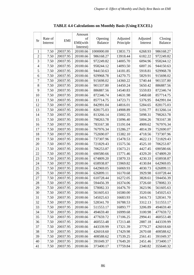
Chapter-4: Effect of Monthly and Daily Rest Basis on EMI
86
TABLE 4.4 Calculations on Monthly Basis (Using EXCEL)
Sr Rate of Interest
EMI
Amount of
EMI(with Interest)
Opening Balance
Adjusted Principle
Adjusted Interest
Closing Balance
1 7.50 20037.95 20100.66 1000000.00 13831.73 6268.93 986168.272 7.50 20037.95 20100.66 986168.27 13918.44 6182.22 972249.823 7.50 20037.95 20100.66 972249.82 14005.70 6094.96 958244.124 7.50 20037.95 20100.66 958244.12 14093.50 6007.16 944150.635 7.50 20037.95 20100.66 944150.63 14181.85 5918.81 929968.786 7.50 20037.95 20100.66 929968.78 14270.75 5829.91 915698.027 7.50 20037.95 20100.66 915698.02 14360.22 5740.44 901337.808 7.50 20037.95 20100.66 901337.80 14450.24 5650.42 886887.569 7.50 20037.95 20100.66 886887.56 14540.83 5559.83 872346.74
10 7.50 20037.95 20100.66 872346.74 14631.98 5468.68 857714.7511 7.50 20037.95 20100.66 857714.75 14723.71 5376.95 842991.0412 7.50 20037.95 20100.66 842991.04 14816.01 5284.65 828175.0313 7.50 20037.95 20100.66 828175.03 14908.89 5191.77 813266.1414 7.50 20037.95 20100.66 813266.14 15002.35 5098.31 798263.7815 7.50 20037.95 20100.66 798263.78 15096.40 5004.26 783167.3816 7.50 20037.95 20100.66 783167.38 15191.04 4909.62 767976.3417 7.50 20037.95 20100.66 767976.34 15286.27 4814.39 752690.0718 7.50 20037.95 20100.66 752690.07 15382.10 4718.56 737307.9619 7.50 20037.95 20100.66 737307.96 15478.53 4622.13 721829.4320 7.50 20037.95 20100.66 721829.43 15575.56 4525.10 706253.8721 7.50 20037.95 20100.66 706253.87 15673.21 4427.45 690580.6622 7.50 20037.95 20100.66 690580.66 15771.46 4329.20 674809.2023 7.50 20037.95 20100.66 674809.20 15870.33 4230.33 658938.8724 7.50 20037.95 20100.66 658938.87 15969.82 4130.84 642969.0525 7.50 20037.95 20100.66 642969.05 16069.93 4030.73 626899.1126 7.50 20037.95 20100.66 626899.11 16170.68 3929.98 610728.4427 7.50 20037.95 20100.66 610728.44 16272.05 3828.61 594456.3928 7.50 20037.95 20100.66 594456.39 16374.06 3726.60 578082.3329 7.50 20037.95 20100.66 578082.33 16476.70 3623.96 561605.6330 7.50 20037.95 20100.66 561605.63 16580.00 3520.66 545025.6331 7.50 20037.95 20100.66 545025.63 16683.93 3416.73 528341.7032 7.50 20037.95 20100.66 528341.70 16788.53 3312.13 511553.1733 7.50 20037.95 20100.66 511553.17 16893.77 3206.89 494659.4034 7.50 20037.95 20100.66 494659.40 16999.68 3100.98 477659.7235 7.50 20037.95 20100.66 477659.72 17106.25 2994.41 460553.4836 7.50 20037.95 20100.66 460553.48 17213.48 2887.18 443339.9937 7.50 20037.95 20100.66 443339.99 17321.39 2779.27 426018.6038 7.50 20037.95 20100.66 426018.60 17429.98 2670.68 408588.6239 7.50 20037.95 20100.66 408588.62 17539.25 2561.41 391049.3740 7.50 20037.95 20100.66 391049.37 17649.20 2451.46 373400.1741 7.50 20037.95 20100.66 373400.17 17759.84 2340.82 355640.32
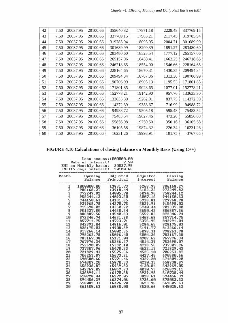
Chapter-4: Effect of Monthly and Daily Rest Basis on EMI
87
42 7.50 20037.95 20100.66 355640.32 17871.18 2229.48 337769.1543 7.50 20037.95 20100.66 337769.15 17983.21 2117.45 319785.9444 7.50 20037.95 20100.66 319785.94 18095.95 2004.71 301689.9945 7.50 20037.95 20100.66 301689.99 18209.39 1891.27 283480.6046 7.50 20037.95 20100.66 283480.60 18323.54 1777.12 265157.0647 7.50 20037.95 20100.66 265157.06 18438.41 1662.25 246718.6548 7.50 20037.95 20100.66 246718.65 18554.00 1546.66 228164.6549 7.50 20037.95 20100.66 228164.65 18670.31 1430.35 209494.3450 7.50 20037.95 20100.66 209494.34 18787.36 1313.30 190706.9951 7.50 20037.95 20100.66 190706.99 18905.13 1195.53 171801.8552 7.50 20037.95 20100.66 171801.85 19023.65 1077.01 152778.2153 7.50 20037.95 20100.66 152778.21 19142.90 957.76 133635.3054 7.50 20037.95 20100.66 133635.30 19262.91 837.75 114372.3955 7.50 20037.95 20100.66 114372.39 19383.67 716.99 94988.7256 7.50 20037.95 20100.66 94988.72 19505.18 595.48 75483.5457 7.50 20037.95 20100.66 75483.54 19627.46 473.20 55856.0858 7.50 20037.95 20100.66 55856.08 19750.50 350.16 36105.5859 7.50 20037.95 20100.66 36105.58 19874.32 226.34 16231.2660 7.50 20037.95 20100.66 16231.26 19998.91 101.75 -3767.65
FIGURE 4.10 Calculations of closing balance on Monthly Basis (Using C++)

Chapter-4: Effect of Monthly and Daily Rest Basis on EMI
88
From the table 4.8 and figure 4.10, it is clear that customer is repaying Rs.3767.65
more for this case when EMI is calculated on monthly compounding basis.
Following is the Excel worksheet based on EMI Rs. 19988.00, calculated on daily
basis for 5 years.
TABLE 4.5 Calculations on Daily Basis (Using EXCEL)
Sr Rate of Interest
EMI
Amount of
EMI(with Interest)
Opening Balance
Adjusted Principle
Adjusted Interest
Closing Balance
1 7.50 19988.22 20050.77 1000000.00 13781.85 6268.93 986218.152 7.50 19988.22 20050.77 986218.15 13868.25 6182.53 972349.913 7.50 19988.22 20050.77 972349.91 13955.18 6095.59 958394.724 7.50 19988.22 20050.77 958394.72 14042.67 6008.11 944352.055 7.50 19988.22 20050.77 944352.05 14130.70 5920.07 930221.356 7.50 19988.22 20050.77 930221.35 14219.29 5831.49 916002.067 7.50 19988.22 20050.77 916002.06 14308.43 5742.35 901693.648 7.50 19988.22 20050.77 901693.64 14398.12 5652.65 887295.529 7.50 19988.22 20050.77 887295.52 14488.38 5562.39 872807.13
10 7.50 19988.22 20050.77 872807.13 14579.21 5471.56 858227.9211 7.50 19988.22 20050.77 858227.92 14670.61 5380.17 843557.3112 7.50 19988.22 20050.77 843557.31 14762.58 5288.20 828794.7413 7.50 19988.22 20050.77 828794.74 14855.12 5195.65 813939.6114 7.50 19988.22 20050.77 813939.61 14948.25 5102.53 798991.3715 7.50 19988.22 20050.77 798991.37 15041.96 5008.82 783949.4116 7.50 19988.22 20050.77 783949.41 15136.25 4914.52 768813.16

Chapter-4: Effect of Monthly and Daily Rest Basis on EMI
89
17 7.50 19988.22 20050.77 768813.16 15231.14 4819.63 753582.0218 7.50 19988.22 20050.77 753582.02 15326.62 4724.15 738255.3919 7.50 19988.22 20050.77 738255.39 15422.71 4628.07 722832.6820 7.50 19988.22 20050.77 722832.68 15519.39 4531.38 707313.2921 7.50 19988.22 20050.77 707313.29 15616.68 4434.09 691696.6222 7.50 19988.22 20050.77 691696.62 15714.58 4336.19 675982.0423 7.50 19988.22 20050.77 675982.04 15813.09 4237.68 660168.9424 7.50 19988.22 20050.77 660168.94 15912.22 4138.55 644256.7225 7.50 19988.22 20050.77 644256.72 16011.98 4038.80 628244.7426 7.50 19988.22 20050.77 628244.74 16112.35 3938.42 612132.3927 7.50 19988.22 20050.77 612132.39 16213.36 3837.41 595919.0228 7.50 19988.22 20050.77 595919.02 16315.00 3735.77 579604.0229 7.50 19988.22 20050.77 579604.02 16417.28 3633.49 563186.7430 7.50 19988.22 20050.77 563186.74 16520.20 3530.58 546666.5431 7.50 19988.22 20050.77 546666.54 16623.76 3427.01 530042.7832 7.50 19988.22 20050.77 530042.78 16727.98 3322.80 513314.8133 7.50 19988.22 20050.77 513314.81 16832.84 3217.93 496481.9634 7.50 19988.22 20050.77 496481.96 16938.37 3112.41 479543.6035 7.50 19988.22 20050.77 479543.60 17044.55 3006.22 462499.0536 7.50 19988.22 20050.77 462499.05 17151.40 2899.37 445347.6537 7.50 19988.22 20050.77 445347.65 17258.92 2791.85 428088.7238 7.50 19988.22 20050.77 428088.72 17367.12 2683.66 410721.6039 7.50 19988.22 20050.77 410721.60 17475.99 2574.78 393245.6140 7.50 19988.22 20050.77 393245.61 17585.55 2465.23 375660.0741 7.50 19988.22 20050.77 375660.07 17695.79 2354.99 357964.2842 7.50 19988.22 20050.77 357964.28 17806.72 2244.05 340157.5543 7.50 19988.22 20050.77 340157.55 17918.35 2132.42 322239.2044 7.50 19988.22 20050.77 322239.20 18030.68 2020.09 304208.5245 7.50 19988.22 20050.77 304208.52 18143.71 1907.06 286064.8146 7.50 19988.22 20050.77 286064.81 18257.46 1793.32 267807.3547 7.50 19988.22 20050.77 267807.35 18371.91 1678.86 249435.4448 7.50 19988.22 20050.77 249435.44 18487.08 1563.69 230948.3649 7.50 19988.22 20050.77 230948.36 18602.98 1447.80 212345.3850 7.50 19988.22 20050.77 212345.38 18719.60 1331.18 193625.7951 7.50 19988.22 20050.77 193625.79 18836.95 1213.83 174788.8452 7.50 19988.22 20050.77 174788.84 18955.04 1095.74 155833.8053 7.50 19988.22 20050.77 155833.80 19073.86 976.91 136759.9454 7.50 19988.22 20050.77 136759.94 19193.44 857.34 117566.5055 7.50 19988.22 20050.77 117566.50 19313.76 737.02 98252.7456 7.50 19988.22 20050.77 98252.74 19434.84 615.94 78817.9157 7.50 19988.22 20050.77 78817.91 19556.67 494.10 59261.2458 7.50 19988.22 20050.77 59261.24 19679.27 371.50 39581.9759 7.50 19988.22 20050.77 39581.97 19802.64 248.14 19779.3360 7.50 19988.22 20050.77 19779.33 19926.78 124.00 -147.45
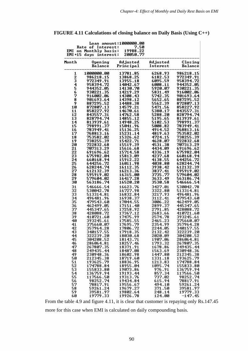
Chapter-4: Effect of Monthly and Daily Rest Basis on EMI
90
FIGURE 4.11 Calculations of closing balance on Daily Basis (Using C++)
From the table 4.9 and figure 4.11, it is clear that customer is repaying only Rs.147.45
more for this case when EMI is calculated on daily compounding basis.

Chapter-4: Effect of Monthly and Daily Rest Basis on EMI
91
Following is the output of ‘emichkal.cpp’, showing Summary of closing balances for
both the methods after completion of various durations is as under:
FIGURE 4.12
From above figure 4.12, we have prepared an Excel worksheet ‘EMI check all.xls’
given as under:
Closing Balance Rest Basis
EMI Number of installments
Total Repayment Amount
Extra % on loan amount
20037.95 60 1202277.00 -3767.65 0.38
11870.18 120 1424421.60 -4506.39 0.45
9270.12 180 1668621.60 -5340.63 0.53 Monthly
8055.93 240 1933423.20 -6284.01 0.63
19988.22 60 1199293.20 -147.45 0.01
11846.16 120 1421539.20 -213.73 0.02
9255.01 180 1665901.80 -311.85 0.03 Daily
8045.46 240 1930910.40 -452.05 0.05
Here, in principle, after completion of all instalments the closing balance amount
should be 0. But considering rounding errors and other points like 365 days in a year,
the amount of closing balance is approaching to 0.
Thus EMI calculated based on daily basis is the proper one.

Chapter-5: Effect of Rest Basis on Bank Deposits
92
Chapter
5 Effect of Rest Basis on Bank Deposits
5.1 INTRODUCTION
Banks are also called custodians of public money. Basically, the money is accepted as
deposit for safe keeping. Since the Banks use this money to earn interest from people
who need money, Banks share a part of this interest with the depositors. The quantum
of interest depends upon the term - length of time for which the depositor wishes to
keep the money with the Bank so to make withdrawal.
A fixed deposit is meant for those investors who want to deposit a lump sum of
money for a fixed period; say for a minimum period of 15 days to five years and
above, thereby earning a higher rate of interest in return. Investor gets a lump sum
(principal + interest) at the maturity of the deposit.
One can calculate maturity amount using different methods of compounding. Here in
this chapter we have calculated maturity amounts of fixed deposits and recurring
deposits using method of quarterly compounding and method of daily compounding.
We have also found the difference amount by using both the methods.
5.1.1 FEATURES
Bank deposits are fairly safe because banks are subject to control of the Reserve Bank
of India (RBI) with regard to several policy and operational parameters. The banks are
free to offer varying interests in fixed deposits of different maturities. Interest is
compounded once a quarter, leading to a somewhat higher effective rate.

Chapter-5: Effect of Rest Basis on Bank Deposits
93
5.1.2 RETURNS
The rate of interest for Bank Fixed Deposits varies between 4 and 11 per cent,
depending on the maturity period (duration) of the FD and the amount invested.
Interest rate also varies between each bank. A Bank FD does not provide regular
interest income, but a lump-sum amount on its maturity. Some banks have facility to
pay interest every quarter or every month, but the interest paid may be at a discounted
rate in case of monthly interest. The Interest payable on Fixed Deposit can also be
transferred to Savings Bank or Current Account of the customer. The deposit period
can vary from 15, 30 or 45 days to 3, 6 months, 1 year, 1.5 years to 10 years.
Duration Interest rate (%) per annum 15-30 days 4 -5 % 30-45 days 4.25-5 % 46-90 days 4.75—5.5 % 91-180 days 5.5-6.5 % 181-365 days 5.75-6.5 % 1-2 years 6-8 % 2-3 years 6.25-8 % 3-5 years 6.75-8
Indian Banks’ Association (IBA) Code for Banking Practice is issued by IBA for
uniform adoption by the Member Banks. The Code is intended to promote good
banking practices by setting out minimum standards which Member Banks will follow
in their dealings with customers. IBA, for the purpose of calculation of interest on
domestic term deposit, have prescribed that on deposits repayable in less than three
months or where the terminal quarter is incomplete, interest should be paid
proportionately for the actual number of days reckoning the year at 365/ 366 days.
5.1.3 BENEFITS, DRAWBACKS AND PRECAUTIONS
Any investment portfolio should comprise the right of safe, moderate and risky
investments. Mutual funds and stocks are the favorite contenders for moderate and
risky investments. Fixed deposits, government bonds etc. are considered safe
investments. Fixed deposits have been particularly popular among a large section of
investors in India as a safe investment option for a long period.
Chapter-5: Effect of Rest Basis on Bank Deposits
94
With fixed deposits or FDs as they are popularly known, a person can invest an
amount for a fixed duration. The banks provide interest rates depending on this loan
amount and the term of deposit. Here are the benefits, drawbacks of fixed deposits and
precautions one should take while making such investments.
5.1.3.1 BENEFITS
Safety: The fixed deposits of reputed banks and financial institutions regulated
by RBI (Reserve Bank of India) the banking regulator in India are very secure
and considered as one of the safest investment methods.
Regular Income: Fixed deposits earn fixed interest rates for their entire
tenure, which is usually compounded quarterly. So, those who want an income
on a regular basis can invest into fixed deposits and use the interest rate as
their income. This makes a fixed deposit very popular way of investing money
for retirees.
Saves tax: With the directives of the income tax department stating that
investment in fixed deposits up to a maximum of Rs.100,000 for 5 years are
eligible for tax deductions under section 80 C of income tax act, fixed deposits
have again become popular. Fixed deposits save tax and give high returns on
invested money.
5.1.3.2 DRAWBACKS
Lower rate of returns: While the money invested in stock markets may give
you a return of 20% the fixed deposits will yield only about 7.5%. So, the
money grows slowly in the case of fixed deposits.
Taxes: The interest earned on fixed deposits is fully taxable and is added to
the annual income of the individual. Gains from stocks are considered capital
gains while dividends are tax free.
Rising inflation can wipe out the interest benefits: The actual benefits or
income from fixed deposit can be annulled by a rising inflation. Suppose the
inflation which is currently at 3 % rises to about 6%, your fixed deposit at
7.5% annual return will effectively yield only(7.5%-6%) = 1.5% of return.
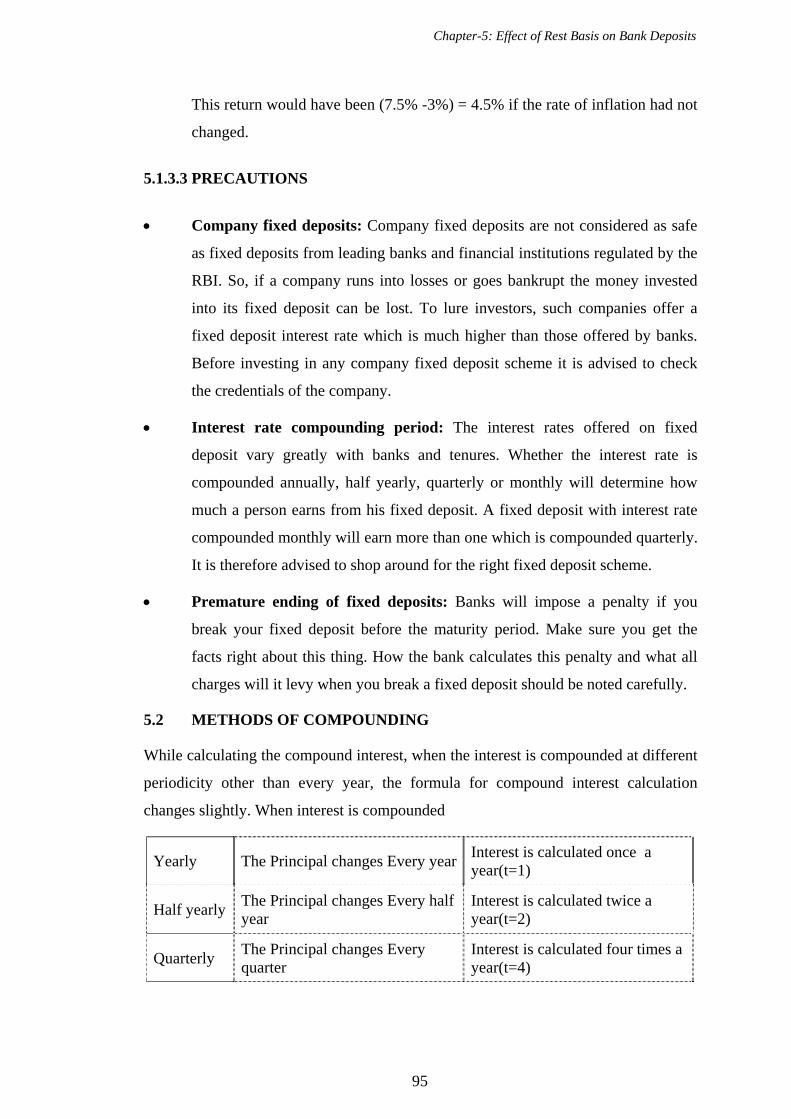
Chapter-5: Effect of Rest Basis on Bank Deposits
95
This return would have been (7.5% -3%) = 4.5% if the rate of inflation had not
changed.
5.1.3.3 PRECAUTIONS
Company fixed deposits: Company fixed deposits are not considered as safe
as fixed deposits from leading banks and financial institutions regulated by the
RBI. So, if a company runs into losses or goes bankrupt the money invested
into its fixed deposit can be lost. To lure investors, such companies offer a
fixed deposit interest rate which is much higher than those offered by banks.
Before investing in any company fixed deposit scheme it is advised to check
the credentials of the company.
Interest rate compounding period: The interest rates offered on fixed
deposit vary greatly with banks and tenures. Whether the interest rate is
compounded annually, half yearly, quarterly or monthly will determine how
much a person earns from his fixed deposit. A fixed deposit with interest rate
compounded monthly will earn more than one which is compounded quarterly.
It is therefore advised to shop around for the right fixed deposit scheme.
Premature ending of fixed deposits: Banks will impose a penalty if you
break your fixed deposit before the maturity period. Make sure you get the
facts right about this thing. How the bank calculates this penalty and what all
charges will it levy when you break a fixed deposit should be noted carefully.
5.2 METHODS OF COMPOUNDING
While calculating the compound interest, when the interest is compounded at different
periodicity other than every year, the formula for compound interest calculation
changes slightly. When interest is compounded
Yearly The Principal changes Every yearInterest is calculated once a year(t=1)
Half yearly The Principal changes Every half year
Interest is calculated twice a year(t=2)
Quarterly The Principal changes Every quarter
Interest is calculated four times a year(t=4)
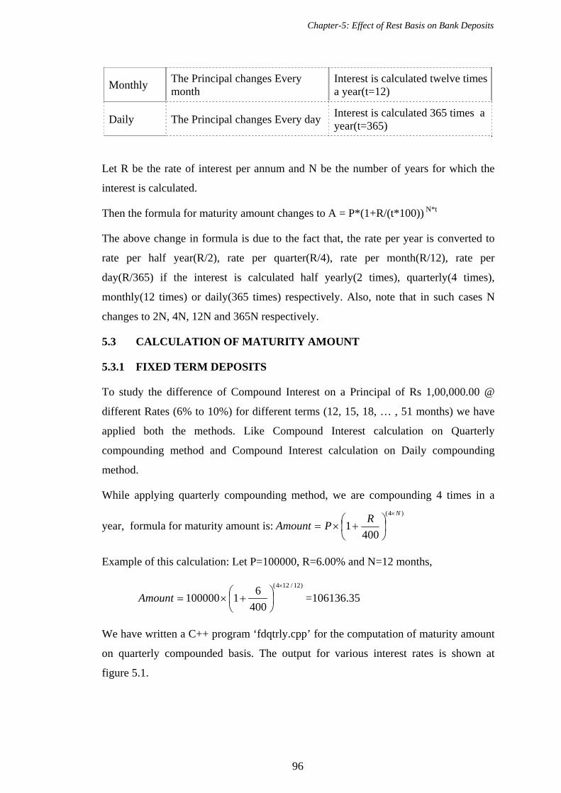
Chapter-5: Effect of Rest Basis on Bank Deposits
96
Monthly The Principal changes Every month
Interest is calculated twelve times a year(t=12)
Daily The Principal changes Every day Interest is calculated 365 times a year(t=365)
Let R be the rate of interest per annum and N be the number of years for which the
interest is calculated.
Then the formula for maturity amount changes to A = P*(1+R/(t*100)) N*t
The above change in formula is due to the fact that, the rate per year is converted to
rate per half year(R/2), rate per quarter(R/4), rate per month(R/12), rate per
day(R/365) if the interest is calculated half yearly(2 times), quarterly(4 times),
monthly(12 times) or daily(365 times) respectively. Also, note that in such cases N
changes to 2N, 4N, 12N and 365N respectively.
5.3 CALCULATION OF MATURITY AMOUNT
5.3.1 FIXED TERM DEPOSITS
To study the difference of Compound Interest on a Principal of Rs 1,00,000.00 @
different Rates (6% to 10%) for different terms (12, 15, 18, … , 51 months) we have
applied both the methods. Like Compound Interest calculation on Quarterly
compounding method and Compound Interest calculation on Daily compounding
method.
While applying quarterly compounding method, we are compounding 4 times in a
year, formula for maturity amount is:)4(
4001
NR
PAmount
Example of this calculation: Let P=100000, R=6.00% and N=12 months,
)12/124(
400
61100000
Amount =106136.35
We have written a C++ program ‘fdqtrly.cpp’ for the computation of maturity amount
on quarterly compounded basis. The output for various interest rates is shown at
figure 5.1.
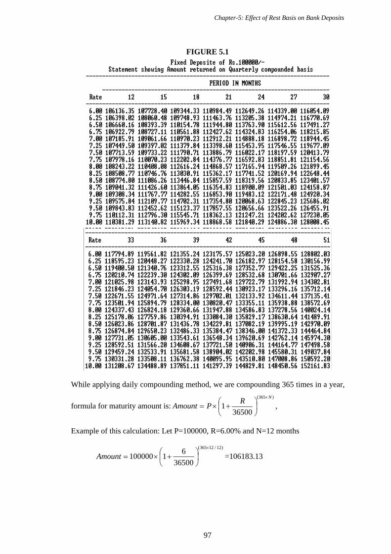
Chapter-5: Effect of Rest Basis on Bank Deposits
97
FIGURE 5.1
While applying daily compounding method, we are compounding 365 times in a year,
formula for maturity amount is:)365(
365001
NR
PAmount
,
Example of this calculation: Let P=100000, R=6.00% and N=12 months
)12/12365(
36500
61100000
Amount =106183.13

Chapter-5: Effect of Rest Basis on Bank Deposits
98
We have written a C++ program ‘fddaily.cpp’ for the computation of maturity amount
on daily compounded basis. The output for various interest rates is shown at figure
5.2.
FIGURE 5.2
When bank is applying method of compounding quarterly, it is useful to know the
difference of maturity amount with compounding daily.
We have written a C++ program ‘fddiff.cpp’ for the computation of difference of
maturity amount on quarterly compounded basis and daily compounded basis. The
output for various interest rates is shown at figure 5.3.

Chapter-5: Effect of Rest Basis on Bank Deposits
99
FIGURE 5.3
Using worksheet of Excel ‘FD-compounding quarterly and daily.xls’, following table
shows the summary of the difference, on P=1,00,000.00, R=7.5% for the years 1 to
10.
TABLE 5.1 Summary of the difference of maturity amount
Interest Amount (Rs.) No. of
Years Compounding
QuarterlyCompounding
Monthly Difference 1 7713.59 7787.58 74.00 2 16022.17 16181.63 159.47 3 24971.64 25229.38 257.74 4 34611.43 34981.72 370.29 5 44994.80 45493.54 498.73 6 56179.10 56823.97 644.87 7 68226.11 69036.77 810.66 8 81202.38 82200.65 998.27 9 95179.58 96389.68 1210.10
10 110234.93 111683.69 1448.76 We can show the above difference graphically as under:

Chapter-5: Effect of Rest Basis on Bank Deposits
100
CHART 5.1
DIFFERENCE OF MATURITY AMOUNT(Compounding daily - Compounding quarterly)
74.00
159.47
257.74
370.29
498.73
644.87
810.66
998.27
1210.10
1448.76
0.00
100.00
200.00
300.00
400.00
500.00
600.00
700.00
800.00
900.00
1000.00
1100.00
1200.00
1300.00
1400.00
1500.00
1600.00
1 2 3 4 5 6 7 8 9 10
YEARS
DIF
FE
RE
NC
E A
MO
UN
T
From chart 5.1 it is clear that while calculating maturity amount using daily
compounding and quarterly compounding methods, the difference of maturity amount
increases rapidly with years for a certain rate of interest.
5.3.2 RECURRING TERM DEPOSIT
Recurring term deposit is a very good investment option to the investors who do not
want to invest the amount at a time for long term but those who want to invest certain
amount every month for certain fixed term.
We have written C++ programs ‘recurqfl.cpp’ and ‘recurdfl.cpp’ to generate a text
file output when the principal amount deposited every month is Rs.100 for various
rates of interests and various terms using compounding quarterly and compounding
daily respectively. We have also written a program called ‘recudiff.cpp’ to generate
the difference table of maturity amounts using compounded daily and compounded
quarterly. Here generated tabulated text file is showing output of maturity amount for
3, 6, 9, …60 months at different rate of interests.
Calculation of maturity amount for the recurring of Rs.100, duration of n months and
quarterly compounding basis or daily compounding basis is given as an example.

Chapter-5: Effect of Rest Basis on Bank Deposits
101
for the 1st month, interest will be calculated on Rs.100 for n months. i.e.
Interest1=12
4
4001100
n
R
OR Interest1=
12365
365001100
n
R
for the 2nd month, interest will be calculated on Rs.100 for (n-1) months. i.e.
Interest2=12
)1(4
4001100
n
R OR Interest2=
12
)1(365
365001100
n
R
Similarly for the nth month, interest will be calculated on Rs.100 for 1 month. i.e.
Interestn=12
14
4001100
R OR Interestn=
12
1365
365001100
R
So, Maturity amount after n months=100n + Interest1 + Interest2 + …. + Interestn
Using above mentioned method we have applied the formula of compounding
quarterly and generated the output text file using C++ program named ‘recurqfl.cpp’.
The generated output is shown at Table 5.2.
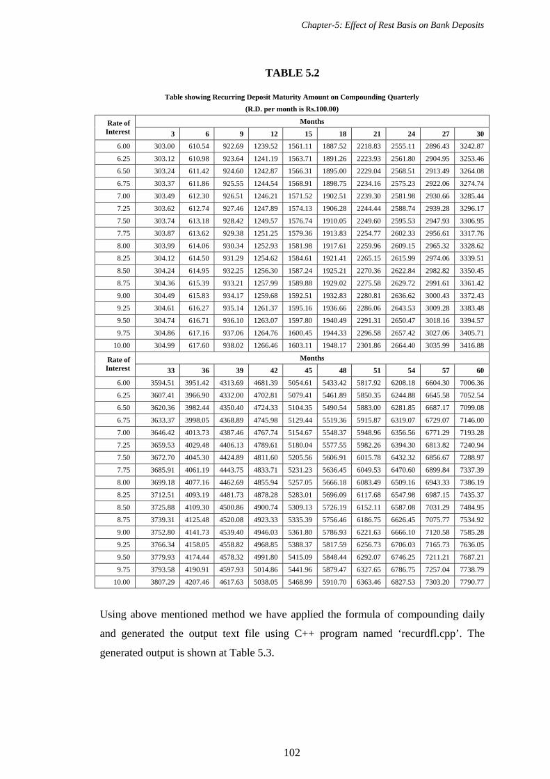
Chapter-5: Effect of Rest Basis on Bank Deposits
102
TABLE 5.2
Table showing Recurring Deposit Maturity Amount on Compounding Quarterly
(R.D. per month is Rs.100.00)
Months Rate of Interest 3 6 9 12 15 18 21 24 27 30
6.00 303.00 610.54 922.69 1239.52 1561.11 1887.52 2218.83 2555.11 2896.43 3242.87
6.25 303.12 610.98 923.64 1241.19 1563.71 1891.26 2223.93 2561.80 2904.95 3253.46
6.50 303.24 611.42 924.60 1242.87 1566.31 1895.00 2229.04 2568.51 2913.49 3264.08
6.75 303.37 611.86 925.55 1244.54 1568.91 1898.75 2234.16 2575.23 2922.06 3274.74
7.00 303.49 612.30 926.51 1246.21 1571.52 1902.51 2239.30 2581.98 2930.66 3285.44
7.25 303.62 612.74 927.46 1247.89 1574.13 1906.28 2244.44 2588.74 2939.28 3296.17
7.50 303.74 613.18 928.42 1249.57 1576.74 1910.05 2249.60 2595.53 2947.93 3306.95
7.75 303.87 613.62 929.38 1251.25 1579.36 1913.83 2254.77 2602.33 2956.61 3317.76
8.00 303.99 614.06 930.34 1252.93 1581.98 1917.61 2259.96 2609.15 2965.32 3328.62
8.25 304.12 614.50 931.29 1254.62 1584.61 1921.41 2265.15 2615.99 2974.06 3339.51
8.50 304.24 614.95 932.25 1256.30 1587.24 1925.21 2270.36 2622.84 2982.82 3350.45
8.75 304.36 615.39 933.21 1257.99 1589.88 1929.02 2275.58 2629.72 2991.61 3361.42
9.00 304.49 615.83 934.17 1259.68 1592.51 1932.83 2280.81 2636.62 3000.43 3372.43
9.25 304.61 616.27 935.14 1261.37 1595.16 1936.66 2286.06 2643.53 3009.28 3383.48
9.50 304.74 616.71 936.10 1263.07 1597.80 1940.49 2291.31 2650.47 3018.16 3394.57
9.75 304.86 617.16 937.06 1264.76 1600.45 1944.33 2296.58 2657.42 3027.06 3405.71
10.00 304.99 617.60 938.02 1266.46 1603.11 1948.17 2301.86 2664.40 3035.99 3416.88
Months Rate of Interest 33 36 39 42 45 48 51 54 57 60
6.00 3594.51 3951.42 4313.69 4681.39 5054.61 5433.42 5817.92 6208.18 6604.30 7006.36
6.25 3607.41 3966.90 4332.00 4702.81 5079.41 5461.89 5850.35 6244.88 6645.58 7052.54
6.50 3620.36 3982.44 4350.40 4724.33 5104.35 5490.54 5883.00 6281.85 6687.17 7099.08
6.75 3633.37 3998.05 4368.89 4745.98 5129.44 5519.36 5915.87 6319.07 6729.07 7146.00
7.00 3646.42 4013.73 4387.46 4767.74 5154.67 5548.37 5948.96 6356.56 6771.29 7193.28
7.25 3659.53 4029.48 4406.13 4789.61 5180.04 5577.55 5982.26 6394.30 6813.82 7240.94
7.50 3672.70 4045.30 4424.89 4811.60 5205.56 5606.91 6015.78 6432.32 6856.67 7288.97
7.75 3685.91 4061.19 4443.75 4833.71 5231.23 5636.45 6049.53 6470.60 6899.84 7337.39
8.00 3699.18 4077.16 4462.69 4855.94 5257.05 5666.18 6083.49 6509.16 6943.33 7386.19
8.25 3712.51 4093.19 4481.73 4878.28 5283.01 5696.09 6117.68 6547.98 6987.15 7435.37
8.50 3725.88 4109.30 4500.86 4900.74 5309.13 5726.19 6152.11 6587.08 7031.29 7484.95
8.75 3739.31 4125.48 4520.08 4923.33 5335.39 5756.46 6186.75 6626.45 7075.77 7534.92
9.00 3752.80 4141.73 4539.40 4946.03 5361.80 5786.93 6221.63 6666.10 7120.58 7585.28
9.25 3766.34 4158.05 4558.82 4968.85 5388.37 5817.59 6256.73 6706.03 7165.73 7636.05
9.50 3779.93 4174.44 4578.32 4991.80 5415.09 5848.44 6292.07 6746.25 7211.21 7687.21
9.75 3793.58 4190.91 4597.93 5014.86 5441.96 5879.47 6327.65 6786.75 7257.04 7738.79
10.00 3807.29 4207.46 4617.63 5038.05 5468.99 5910.70 6363.46 6827.53 7303.20 7790.77
Using above mentioned method we have applied the formula of compounding daily
and generated the output text file using C++ program named ‘recurdfl.cpp’. The
generated output is shown at Table 5.3.
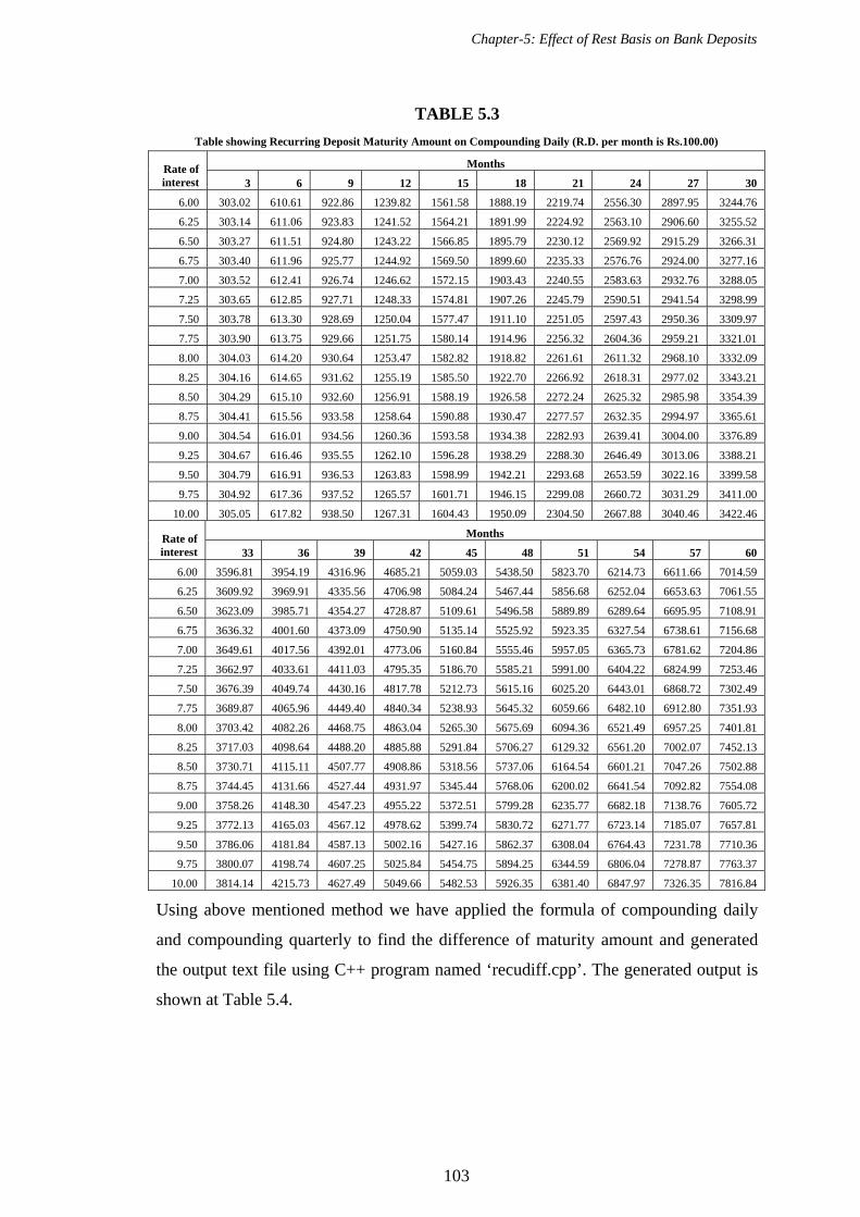
Chapter-5: Effect of Rest Basis on Bank Deposits
103
TABLE 5.3
Table showing Recurring Deposit Maturity Amount on Compounding Daily (R.D. per month is Rs.100.00)
Months Rate of interest 3 6 9 12 15 18 21 24 27 30
6.00 303.02 610.61 922.86 1239.82 1561.58 1888.19 2219.74 2556.30 2897.95 3244.76
6.25 303.14 611.06 923.83 1241.52 1564.21 1891.99 2224.92 2563.10 2906.60 3255.52
6.50 303.27 611.51 924.80 1243.22 1566.85 1895.79 2230.12 2569.92 2915.29 3266.31
6.75 303.40 611.96 925.77 1244.92 1569.50 1899.60 2235.33 2576.76 2924.00 3277.16
7.00 303.52 612.41 926.74 1246.62 1572.15 1903.43 2240.55 2583.63 2932.76 3288.05
7.25 303.65 612.85 927.71 1248.33 1574.81 1907.26 2245.79 2590.51 2941.54 3298.99
7.50 303.78 613.30 928.69 1250.04 1577.47 1911.10 2251.05 2597.43 2950.36 3309.97
7.75 303.90 613.75 929.66 1251.75 1580.14 1914.96 2256.32 2604.36 2959.21 3321.01
8.00 304.03 614.20 930.64 1253.47 1582.82 1918.82 2261.61 2611.32 2968.10 3332.09
8.25 304.16 614.65 931.62 1255.19 1585.50 1922.70 2266.92 2618.31 2977.02 3343.21
8.50 304.29 615.10 932.60 1256.91 1588.19 1926.58 2272.24 2625.32 2985.98 3354.39
8.75 304.41 615.56 933.58 1258.64 1590.88 1930.47 2277.57 2632.35 2994.97 3365.61
9.00 304.54 616.01 934.56 1260.36 1593.58 1934.38 2282.93 2639.41 3004.00 3376.89
9.25 304.67 616.46 935.55 1262.10 1596.28 1938.29 2288.30 2646.49 3013.06 3388.21
9.50 304.79 616.91 936.53 1263.83 1598.99 1942.21 2293.68 2653.59 3022.16 3399.58
9.75 304.92 617.36 937.52 1265.57 1601.71 1946.15 2299.08 2660.72 3031.29 3411.00
10.00 305.05 617.82 938.50 1267.31 1604.43 1950.09 2304.50 2667.88 3040.46 3422.46
Months Rate of interest 33 36 39 42 45 48 51 54 57 60
6.00 3596.81 3954.19 4316.96 4685.21 5059.03 5438.50 5823.70 6214.73 6611.66 7014.59
6.25 3609.92 3969.91 4335.56 4706.98 5084.24 5467.44 5856.68 6252.04 6653.63 7061.55
6.50 3623.09 3985.71 4354.27 4728.87 5109.61 5496.58 5889.89 6289.64 6695.95 7108.91
6.75 3636.32 4001.60 4373.09 4750.90 5135.14 5525.92 5923.35 6327.54 6738.61 7156.68
7.00 3649.61 4017.56 4392.01 4773.06 5160.84 5555.46 5957.05 6365.73 6781.62 7204.86
7.25 3662.97 4033.61 4411.03 4795.35 5186.70 5585.21 5991.00 6404.22 6824.99 7253.46
7.50 3676.39 4049.74 4430.16 4817.78 5212.73 5615.16 6025.20 6443.01 6868.72 7302.49
7.75 3689.87 4065.96 4449.40 4840.34 5238.93 5645.32 6059.66 6482.10 6912.80 7351.93
8.00 3703.42 4082.26 4468.75 4863.04 5265.30 5675.69 6094.36 6521.49 6957.25 7401.81
8.25 3717.03 4098.64 4488.20 4885.88 5291.84 5706.27 6129.32 6561.20 7002.07 7452.13
8.50 3730.71 4115.11 4507.77 4908.86 5318.56 5737.06 6164.54 6601.21 7047.26 7502.88
8.75 3744.45 4131.66 4527.44 4931.97 5345.44 5768.06 6200.02 6641.54 7092.82 7554.08
9.00 3758.26 4148.30 4547.23 4955.22 5372.51 5799.28 6235.77 6682.18 7138.76 7605.72
9.25 3772.13 4165.03 4567.12 4978.62 5399.74 5830.72 6271.77 6723.14 7185.07 7657.81
9.50 3786.06 4181.84 4587.13 5002.16 5427.16 5862.37 6308.04 6764.43 7231.78 7710.36
9.75 3800.07 4198.74 4607.25 5025.84 5454.75 5894.25 6344.59 6806.04 7278.87 7763.37
10.00 3814.14 4215.73 4627.49 5049.66 5482.53 5926.35 6381.40 6847.97 7326.35 7816.84
Using above mentioned method we have applied the formula of compounding daily
and compounding quarterly to find the difference of maturity amount and generated
the output text file using C++ program named ‘recudiff.cpp’. The generated output is
shown at Table 5.4.
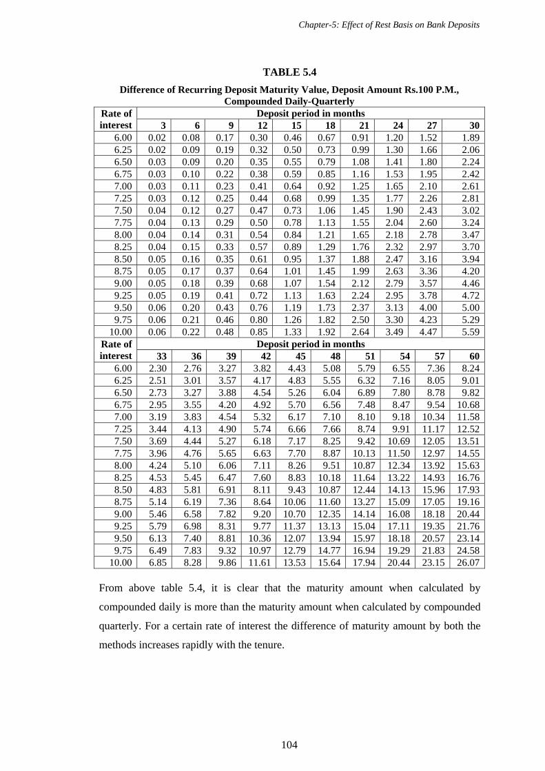
Chapter-5: Effect of Rest Basis on Bank Deposits
104
TABLE 5.4
Difference of Recurring Deposit Maturity Value, Deposit Amount Rs.100 P.M., Compounded Daily-Quarterly
Deposit period in months Rate of interest 3 6 9 12 15 18 21 24 27 30
6.00 0.02 0.08 0.17 0.30 0.46 0.67 0.91 1.20 1.52 1.896.25 0.02 0.09 0.19 0.32 0.50 0.73 0.99 1.30 1.66 2.066.50 0.03 0.09 0.20 0.35 0.55 0.79 1.08 1.41 1.80 2.246.75 0.03 0.10 0.22 0.38 0.59 0.85 1.16 1.53 1.95 2.427.00 0.03 0.11 0.23 0.41 0.64 0.92 1.25 1.65 2.10 2.617.25 0.03 0.12 0.25 0.44 0.68 0.99 1.35 1.77 2.26 2.817.50 0.04 0.12 0.27 0.47 0.73 1.06 1.45 1.90 2.43 3.027.75 0.04 0.13 0.29 0.50 0.78 1.13 1.55 2.04 2.60 3.248.00 0.04 0.14 0.31 0.54 0.84 1.21 1.65 2.18 2.78 3.478.25 0.04 0.15 0.33 0.57 0.89 1.29 1.76 2.32 2.97 3.708.50 0.05 0.16 0.35 0.61 0.95 1.37 1.88 2.47 3.16 3.948.75 0.05 0.17 0.37 0.64 1.01 1.45 1.99 2.63 3.36 4.209.00 0.05 0.18 0.39 0.68 1.07 1.54 2.12 2.79 3.57 4.469.25 0.05 0.19 0.41 0.72 1.13 1.63 2.24 2.95 3.78 4.729.50 0.06 0.20 0.43 0.76 1.19 1.73 2.37 3.13 4.00 5.009.75 0.06 0.21 0.46 0.80 1.26 1.82 2.50 3.30 4.23 5.29
10.00 0.06 0.22 0.48 0.85 1.33 1.92 2.64 3.49 4.47 5.59Deposit period in months Rate of
interest 33 36 39 42 45 48 51 54 57 606.00 2.30 2.76 3.27 3.82 4.43 5.08 5.79 6.55 7.36 8.246.25 2.51 3.01 3.57 4.17 4.83 5.55 6.32 7.16 8.05 9.016.50 2.73 3.27 3.88 4.54 5.26 6.04 6.89 7.80 8.78 9.826.75 2.95 3.55 4.20 4.92 5.70 6.56 7.48 8.47 9.54 10.687.00 3.19 3.83 4.54 5.32 6.17 7.10 8.10 9.18 10.34 11.587.25 3.44 4.13 4.90 5.74 6.66 7.66 8.74 9.91 11.17 12.527.50 3.69 4.44 5.27 6.18 7.17 8.25 9.42 10.69 12.05 13.517.75 3.96 4.76 5.65 6.63 7.70 8.87 10.13 11.50 12.97 14.558.00 4.24 5.10 6.06 7.11 8.26 9.51 10.87 12.34 13.92 15.638.25 4.53 5.45 6.47 7.60 8.83 10.18 11.64 13.22 14.93 16.768.50 4.83 5.81 6.91 8.11 9.43 10.87 12.44 14.13 15.96 17.938.75 5.14 6.19 7.36 8.64 10.06 11.60 13.27 15.09 17.05 19.169.00 5.46 6.58 7.82 9.20 10.70 12.35 14.14 16.08 18.18 20.449.25 5.79 6.98 8.31 9.77 11.37 13.13 15.04 17.11 19.35 21.769.50 6.13 7.40 8.81 10.36 12.07 13.94 15.97 18.18 20.57 23.149.75 6.49 7.83 9.32 10.97 12.79 14.77 16.94 19.29 21.83 24.58
10.00 6.85 8.28 9.86 11.61 13.53 15.64 17.94 20.44 23.15 26.07 From above table 5.4, it is clear that the maturity amount when calculated by
compounded daily is more than the maturity amount when calculated by compounded
quarterly. For a certain rate of interest the difference of maturity amount by both the
methods increases rapidly with the tenure.

Chapter-5: Effect of Rest Basis on Bank Deposits
105
CHART 5.2
Difference of Maturity amount(Compounding Daily - Compounding Quarterly, on Rs.100 @ 7.5% rate of interest)
0.04 0.12 0.27 0.47 0.731.06
1.451.90
2.433.02
3.69
4.44
5.27
6.18
7.17
8.25
9.42
10.69
12.05
13.51
0.00
2.00
4.00
6.00
8.00
10.00
12.00
14.00
16.00
3 6 9 12 15 18 21 24 27 30 33 36 39 42 45 48 51 54 57 60
Period-Months
Diff
eren
ce A
mou
nt
From chart 5.2 it is clear that while calculating maturity amount using daily compounding and quarterly compounding methods, the difference of
maturity amount increases rapidly with tenure for a certain rate of interest.

Chapter-5: Effect of Rest Basis on Bank Deposits
106
We have calculated the difference of maturity amounts for the recurring of Rs.100.
We can obtain the same for any amount of recurring deposit. Let us calculate the
differences for various amounts of deposit amounts per month for the duration of 5
years at 7.5% rate of interest. Summary is shown in Table 5.5.
TABLE 5.5
Deposit amount P.M.
Difference of Maturity Amount
100 13.511000 135.10
10000 1351.0020000 2702.0030000 4053.00
40000 5404.0050000 6755.0060000 8106.0070000 9457.0080000 10808.0090000 12159.00
100000 13510.00
The graph of Deposit amount P.M. Vs. Difference amount is shown at chart 5.3.
CHART 5.3
Deposit amount Vs. Difference amount
135.10
1351.00
2702.00
4053.00
5404.00
6755.00
8106.00
9457.00
10808.00
12159.00
13510.00
0.00
1000.00
2000.00
3000.00
4000.00
5000.00
6000.00
7000.00
8000.00
9000.00
10000.00
11000.00
12000.00
13000.00
14000.00
15000.00
1000 10000 20000 30000 40000 50000 60000 70000 80000 90000 100000
Deposit amount (P.M.)
Dif
fere
nce
of
mat
uri
ty a
mou
nt
Difference Amount
From chart 5.3, it is clear that for the certain rate of interest and tenure, the difference
of maturity amount increases rapidly with the amount deposited per month.
Chapter-5: Effect of Rest Basis on Bank Deposits
107
5.4 DIFFERENCE OF POLICY
While giving loans to the customer, bank is calculating interest on daily compounding
basis, which is comparatively higher than quarterly compounding basis. The same
bank is calculating interest on quarterly compounding basis while taking money as
fixed deposit or recurring deposit.

Chapter-6: Weibull Distribution for Amount Withdrawn Per Day
108
Chapter
6 Weibull Distribution for
Amount Withdrawn Per Day
6.1 INTRODUCTION
In the banking services ATM is playing very important role because it helps to solve
problems for which people do not have to come to bank and wait to withdraw money.
ATM machine contains a paper role in it, on which details of each visit of a customer
is printed. Details are like date, time, amount withdrawn etc. Here in this chapter we
have focused our study on the amount withdrawn per day from the ATM. We have
collected data of hit and amount withdrawn through ATM for 1 year varying from 01-
01-2005 to 31-12-2005.
In this chapter our intension is to fit this data for a distribution. For which we obtained
frequency distribution of amount withdrawn per day with class interval 25000 and
then we draw the graph for number of amount Vs. frequency and found that frequency
distribution is right skewed. Hence in such situation we found that weibull
distribution will fit well.
6.2 FREQUENCY DISTRIBUTION OF AMOUNT WITHDRAWN PER DAY
TABLE 6.1
Lower Limit
Upper Limit Mid value Frequency
1 25000 12500.5 0
25001 50000 37500.5 3
50001 75000 62500.5 7
75001 100000 87500.5 17
100001 125000 112500.5 34
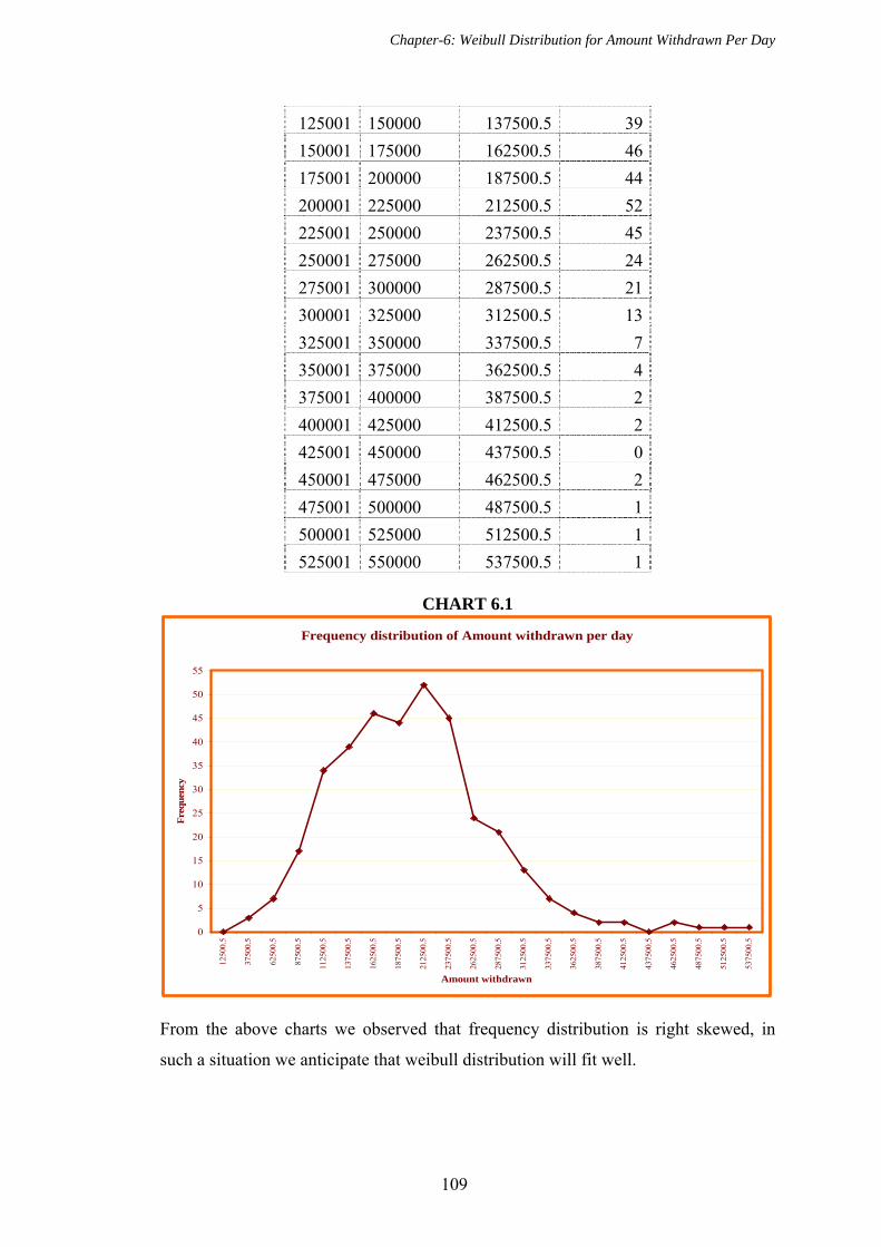
Chapter-6: Weibull Distribution for Amount Withdrawn Per Day
109
125001 150000 137500.5 39
150001 175000 162500.5 46
175001 200000 187500.5 44
200001 225000 212500.5 52
225001 250000 237500.5 45
250001 275000 262500.5 24
275001 300000 287500.5 21
300001 325000 312500.5 13
325001 350000 337500.5 7
350001 375000 362500.5 4
375001 400000 387500.5 2
400001 425000 412500.5 2
425001 450000 437500.5 0
450001 475000 462500.5 2
475001 500000 487500.5 1
500001 525000 512500.5 1
525001 550000 537500.5 1
CHART 6.1
Frequency distribution of Amount withdrawn per day
0
5
10
15
20
25
30
35
40
45
50
55
1250
0.5
3750
0.5
6250
0.5
8750
0.5
1125
00.5
1375
00.5
1625
00.5
1875
00.5
2125
00.5
2375
00.5
2625
00.5
2875
00.5
3125
00.5
3375
00.5
3625
00.5
3875
00.5
4125
00.5
4375
00.5
4625
00.5
4875
00.5
5125
00.5
5375
00.5
Amount withdrawn
Fre
qu
ency
From the above charts we observed that frequency distribution is right skewed, in
such a situation we anticipate that weibull distribution will fit well.
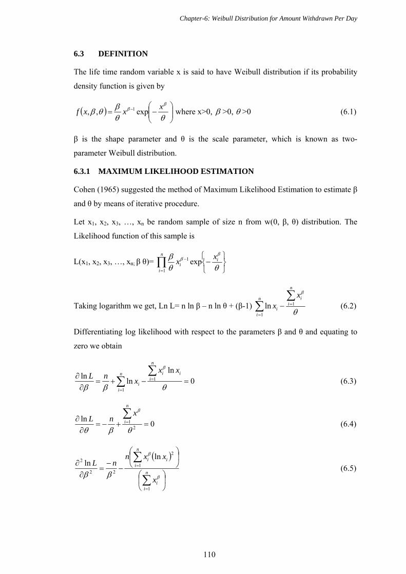
Chapter-6: Weibull Distribution for Amount Withdrawn Per Day
110
6.3 DEFINITION
The life time random variable x is said to have Weibull distribution if its probability
density function is given by
x
xxf exp,, 1 where x>0, >0, >0 (6.1)
β is the shape parameter and θ is the scale parameter, which is known as two-
parameter Weibull distribution.
6.3.1 MAXIMUM LIKELIHOOD ESTIMATION
Cohen (1965) suggested the method of Maximum Likelihood Estimation to estimate β
and θ by means of iterative procedure.
Let x1, x2, x3, …, xn be random sample of size n from w(0, β, θ) distribution. The
Likelihood function of this sample is
L(x1, x2, x3, …, xn; β θ)=
in
ii
xx exp
1
1
Taking logarithm we get, Ln L= n ln β – n ln θ + (β-1)
n
iin
ii
xx 1
1
ln (6.2)
Differentiating log likelihood with respect to the parameters β and θ and equating to
zero we obtain
0ln
lnln
1
1
n
i
n
iii
i
xxx
nL
(6.3)
0ln
21
n
i
xnL
(6.4)
n
ii
n
iii
x
xxnnL
1
1
2
22
2ln
ln
(6.5)
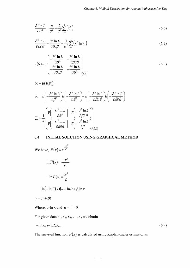
Chapter-6: Weibull Distribution for Amount Withdrawn Per Day
111
n
iix
nL
1322
2 2ln
(6.6)
n
iii xx
LL
12
22
ln1lnln
(6.7)
ˆ,ˆ2
22
2
2
2
lnln
lnln
LL
LL
EI (6.8)
1 IE
ˆˆ
lnˆˆ
lnˆln
ˆln 22
2
2
2
2 LE
LE
LE
LEK
ˆ,ˆ2
22
2
2
2
lnln
lnln
1
LE
LE
LE
LE
K
6.4 INITIAL SOLUTION USING GRAPHICAL METHOD
We have,
x
exF
xxF
ln
xxF ln
xxF lnlnlnln
ty
Where, t=ln x and = -ln
For given data x1, x2, x3, …, xn we obtain
ti=ln xi, i=1,2,3,…. (6.9)
The survival function xF is calculated using Kaplan-meier estimator as

Chapter-6: Weibull Distribution for Amount Withdrawn Per Day
112
1
1ˆ
n
inxF i
Define si )(lnln( )(ixF
))1
1ln(ln(
in
n (6.10)
By taking (si, ti), i=1, 2, 3, …, n, we fit a straight line.
Then estimator of slope (which is same as shape parameter)
2)(
))((ˆtt
ttss
i
ii (6.11)
And
)(,)(
)(,
ˆ
)(
ˆ
censoredr
xrnx
uncensoredn
x
ri
i
(6.12)
To calculate initial solution, we have developed a C++ program named ‘gramt.cpp’.
We are using data files to handle the data. A data file ‘snramta.csv’ consisting fields
like serial number and data observations x1, x2, …, xn (showing amount withdrawn
per day) is created in Excel. We are reading the same and creating one data file to
store our tabulated output. Following is the algorithm for the program:
1. Open input data file ‘snramta.csv’ to read and output data file ‘graphamt.txt’ to
write.
2. Read the input data file ‘snramta.csv’ till end of file and do following till end of
file.
a. Store observation x to array element ax[i] and add to tx for total of x.
b. Calculate
1
1lnln
in
nsi and store in array element as[i] and add to ts
for total.
c. Calculate ii xt ln and store in array element at[i] and add to tt for total.
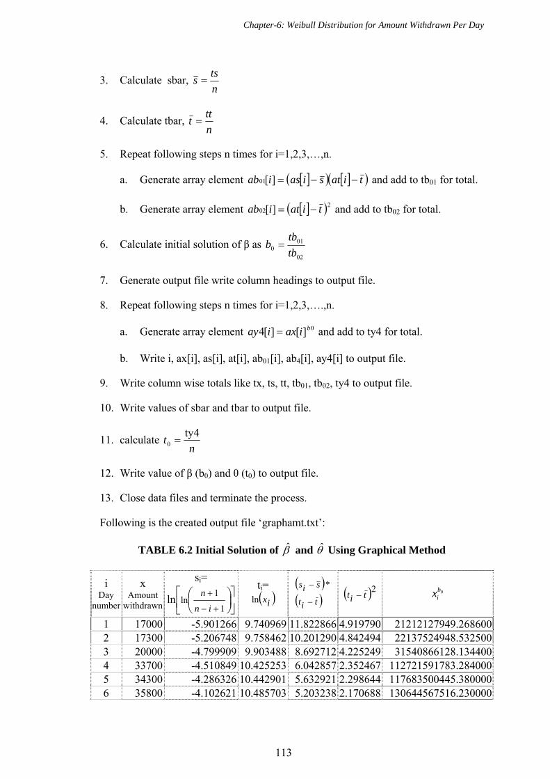
Chapter-6: Weibull Distribution for Amount Withdrawn Per Day
113
3. Calculate sbar, n
tss
4. Calculate tbar, n
ttt
5. Repeat following steps n times for i=1,2,3,…,n.
a. Generate array element tiatsiasiab ][01 and add to tb01 for total.
b. Generate array element 202 ][ tiatiab and add to tb02 for total.
6. Calculate initial solution of β as 02
010 tb
tbb
7. Generate output file write column headings to output file.
8. Repeat following steps n times for i=1,2,3,….,n.
a. Generate array element 0][][4 biaxiay and add to ty4 for total.
b. Write i, ax[i], as[i], at[i], ab01[i], ab4[i], ay4[i] to output file.
9. Write column wise totals like tx, ts, tt, tb01, tb02, ty4 to output file.
10. Write values of sbar and tbar to output file.
11. calculate n
t4ty
0
12. Write value of β (b0) and θ (t0) to output file.
13. Close data files and terminate the process.
Following is the created output file ‘graphamt.txt’:
TABLE 6.2 Initial Solution of and Using Graphical Method
i Day
number
x Amount
withdrawn
si=
1
1lnln
in
nti= ixln
tit
sis
* 2tit 0b
ix
1 17000 -5.901266 9.740969 11.822866 4.919790 21212127949.2686002 17300 -5.206748 9.758462 10.201290 4.842494 22137524948.5325003 20000 -4.799909 9.903488 8.692712 4.225249 31540866128.1344004 33700 -4.510849 10.425253 6.042857 2.352467 112721591783.2840005 34300 -4.286326 10.442901 5.632921 2.298644 117683500445.3800006 35800 -4.102621 10.485703 5.203238 2.170688 130644567516.230000

Chapter-6: Weibull Distribution for Amount Withdrawn Per Day
114
7 36800 -3.947083 10.513253 4.881070 2.090267 139732547901.4790008 37100 -3.812162 10.521372 4.659688 2.066856 142529517451.0360009 40800 -3.692986 10.616437 4.191561 1.802551 179756717809.99200010 49100 -3.586229 10.801614 3.489878 1.339608 282484552995.59000011 51000 -3.489519 10.839581 3.267138 1.253163 309915865573.43200012 51100 -3.401105 10.841540 3.162619 1.248781 311401312593.36500013 51500 -3.319656 10.849337 3.050169 1.231415 317385085389.81400014 51600 -3.244138 10.851277 2.961182 1.227114 318891542830.31700015 53700 -3.173733 10.891168 2.779363 1.140326 351505844663.04800016 53900 -3.107778 10.894886 2.699502 1.132400 354710069486.42700017 59200 -3.045734 10.988677 2.401370 0.941582 445967479080.51800018 60400 -2.987152 11.008744 2.296039 0.903040 468357189873.74500019 61500 -2.931658 11.026792 2.200699 0.869064 489452206015.51900020 62500 -2.878935 11.042922 2.114322 0.839251 509107332086.73900021 63500 -2.828712 11.058795 2.032475 0.810420 529220901227.93300022 67200 -2.780755 11.115429 1.864156 0.711661 607680163307.12800023 67800 -2.734863 11.124317 1.806207 0.696743 621009723587.17800024 70800 -2.690860 11.167614 1.677694 0.626337 690236878270.86000025 72100 -2.648591 11.185809 1.606439 0.597868 721584286929.41200026 72600 -2.607919 11.192720 1.560914 0.587228 733860341961.20200027 74800 -2.568725 11.222573 1.471241 0.542367 789334539968.09600028 76700 -2.530899 11.247657 1.394222 0.506049 839175779551.08000029 77300 -2.494346 11.255449 1.353232 0.495024 855290500917.03400030 78600 -2.458980 11.272127 1.296862 0.471834 890828368896.72100031 79500 -2.424721 11.283512 1.252224 0.456322 915933267726.77000032 79800 -2.391500 11.287279 1.222926 0.451248 924393222611.48800033 79900 -2.359252 11.288531 1.199024 0.449567 927223416009.02600034 83000 -2.327920 11.326596 1.111138 0.399971 1017507348009.16000035 83200 -2.297449 11.329003 1.087713 0.396933 1023502681031.85000036 83500 -2.267791 11.332602 1.062920 0.392410 1032534694398.16000037 83600 -2.238901 11.333799 1.042826 0.390912 1035555780226.94000038 85100 -2.210738 11.351582 0.996058 0.368991 1081499036167.05000039 85800 -2.183264 11.359774 0.966161 0.359106 1103343140487.96000040 86000 -2.156444 11.362103 0.946397 0.356321 1109631720343.00000041 87800 -2.130245 11.382817 0.898460 0.332020 1167181462135.83000042 88200 -2.104638 11.387362 0.876734 0.326802 1180204079418.50000043 88600 -2.079593 11.391887 0.855590 0.321649 1193312081020.27000044 89500 -2.055086 11.401994 0.826692 0.310288 1223118153784.40000045 89900 -2.031092 11.406453 0.806815 0.305339 1236504830120.11000046 90900 -2.007587 11.417515 0.777935 0.293237 1270348604784.47000047 92600 -1.984552 11.436044 0.739269 0.273512 1329125546983.62000048 94100 -1.961965 11.452113 0.705105 0.256963 1382295691239.25000049 95900 -1.939808 11.471061 0.667937 0.238112 1447731477592.09000050 96500 -1.918064 11.477298 0.648925 0.232064 1469941348219.070000
.
.
.

Chapter-6: Weibull Distribution for Amount Withdrawn Per Day
115
315 252100 0.678443 12.437581 0.597921 0.229013 15321945389258.900000316 253000 0.688441 12.441145 0.607193 0.232436 15455811319606.000000317 253600 0.698539 12.443514 0.615069 0.234726 15545437416127.800000318 254200 0.708741 12.445877 0.623036 0.237021 15635369599927.000000319 255400 0.719052 12.450586 0.634131 0.241629 15816153505589.000000320 255600 0.729475 12.451369 0.640273 0.242399 15846403493579.100000321 256500 0.740017 12.454884 0.650071 0.245873 15982950940112.300000322 256600 0.750682 12.455274 0.655874 0.246259 15998165584856.800000323 263800 0.761475 12.482947 0.698104 0.274490 17116171572899.400000324 268600 0.772404 12.500979 0.728053 0.293710 17886391826638.500000325 269300 0.783473 12.503581 0.737577 0.296538 18000390563084.300000326 270000 0.794690 12.506177 0.747231 0.299372 18114817102327.800000327 270100 0.806061 12.506548 0.753963 0.299777 18131198702051.900000328 271300 0.817596 12.510980 0.766434 0.304651 18328460190454.500000329 271800 0.829301 12.512822 0.775473 0.306687 18411024602258.500000330 272800 0.841185 12.516494 0.787240 0.310768 18576811077699.800000331 273200 0.853259 12.517959 0.796058 0.312404 18643371443219.600000332 273700 0.865533 12.519788 0.805545 0.314451 18726769600407.500000333 275300 0.878018 12.525617 0.820992 0.321022 18995121848974.800000334 275700 0.890726 12.527069 0.830314 0.322670 19062562322080.700000335 276600 0.903670 12.530328 0.842473 0.326383 19214819586196.300000336 277300 0.916865 12.532855 0.853772 0.329277 19333736568800.400000337 279100 0.930327 12.539325 0.871211 0.336744 19641514180724.600000338 279600 0.944073 12.541115 0.881899 0.338825 19727517602094.300000339 280500 0.958122 12.544329 0.894991 0.342577 19882883090787.100000340 284100 0.972496 12.557082 0.923088 0.357667 20511555289163.300000341 286000 0.987218 12.563747 0.942278 0.365685 20848021072175.900000342 286200 1.002314 12.564446 0.952507 0.366530 20883626632391.300000343 290200 1.017814 12.578326 0.983943 0.383529 21603285795575.200000344 299200 1.033750 12.608868 1.042824 0.422291 23275437890389.900000345 299800 1.050161 12.610871 1.056736 0.424898 23389537717750.300000346 302100 1.067088 12.618513 1.080289 0.434920 23829975690601.900000347 302200 1.084579 12.618844 1.092372 0.435357 23849235264837.800000348 308900 1.102691 12.640773 1.141024 0.464775 25160619301038.800000349 310300 1.121489 12.645295 1.161492 0.470961 25439885584293.100000350 313500 1.141047 12.655555 1.192480 0.485149 26085054523362.500000351 318900 1.161457 12.672633 1.236283 0.509231 27195477273588.700000352 324900 1.182824 12.691273 1.284221 0.536182 28461459093804.800000353 334000 1.205277 12.718896 1.349730 0.577399 30446782615275.700000354 335400 1.228976 12.723079 1.375266 0.583773 30759249248718.100000355 346000 1.254116 12.754194 1.451263 0.632288 33186484539162.000000356 349000 1.280947 12.762827 1.488586 0.646092 33893265344453.100000357 369400 1.309794 12.819635 1.618617 0.740644 38934696737817.800000358 373100 1.341086 12.829602 1.664604 0.757898 39893521828098.300000359 380730 1.375416 12.849846 1.733894 0.793555 41914414564391.700000360 382900 1.413636 12.855529 1.779220 0.803713 42499955925679.300000361 440900 1.457031 12.996573 2.104165 1.076499 59966973053443.700000362 446300 1.507702 13.008747 2.182042 1.101908 61775639528712.800000

Chapter-6: Weibull Distribution for Amount Withdrawn Per Day
116
363 457300 1.569453 13.033095 2.298980 1.153619 65558543733497.000000364 488700 1.650481 13.099504 2.533536 1.300684 77095834415330.200000365 523100 1.775399 13.167528 2.835612 1.460471 91021559723153.200000TOT 63822850 -208.412057 4365.045414 232.581184 95.280569 3131158681713497.280000
-0.570992 11.959029 Remark: We did not show the entire value of x because of space. If any one require,
we can provide it as we have stored as soft copy. As per given algorithm, we have calculated values of initial solution. i.e. β and θ. β=2.4410138 and θ=8578516936201.362400.
6.5 ESTIMATION OF PARAMETERS BY N-R METHOD
We have written a C++ program ‘nramt.cpp’, to get the final solution using N-R
method. Output is stored in a data file named ‘nramt.txt’.
To write the algorithm let us rewrite equations (6.3) and (6.5) for the reference, as
0ln
lnln
1
1
n
i
n
iii
i
xxx
nL
(6.3)
Equation (6.3) can be rewritten as
0
21
01 t
yy
b
nz
Where, β= b0, θ= t0, y1=
n
iix
1
ln and y2=
n
iii xx
1
ln
n
ii
n
iii
x
xxnnL
1
1
2
22
2ln
ln
(6.5)
Equation (6.5) can be rewritten as
Z2=4
32
0y
ny
b
n Where, β= b0, y3=
n
iii xx
1
2ln and y4=
n
iix
1
Algorithm for the above program ‘nramt.cpp’ is as under:
1. Find the initial solution, i.e., calculate b0 and t0 using graphical method as shown
earlier.

Chapter-6: Weibull Distribution for Amount Withdrawn Per Day
117
2. Calculate y1=
n
iix
1
ln
3. Calculate y2=
n
ii
bi xx
1
ln0
4. Calculate y3=
n
ii
bi xx
1
2ln0
5. Calculate y4=
n
i
bix
1
0
6. Calculate 0
21
01 t
yy
b
nz
7. Calculate z2=4
32
0y
ny
b
n
8. Calculate 2
101 z
zbb
9. Calculate t1=n
y4
10. Calculate the difference between b0 and b1, i.e. difference= abs(b1-b0)
11. Assign value of b1 to b0
12. Repeat above steps 3 to 10 till the difference<= 0.0001
13. Terminate the process.
This is iterative process. To reduce the number of iterations we have taken the initial
solution by graphical method, i.e., nearer to the final solution. Using C++ program we
could get the final solution (with the difference > 0.0001) after 343 iterations. Portion
of tabulated output and solution of last iteration by N-R method using ‘nramt.cpp’
program is as under:
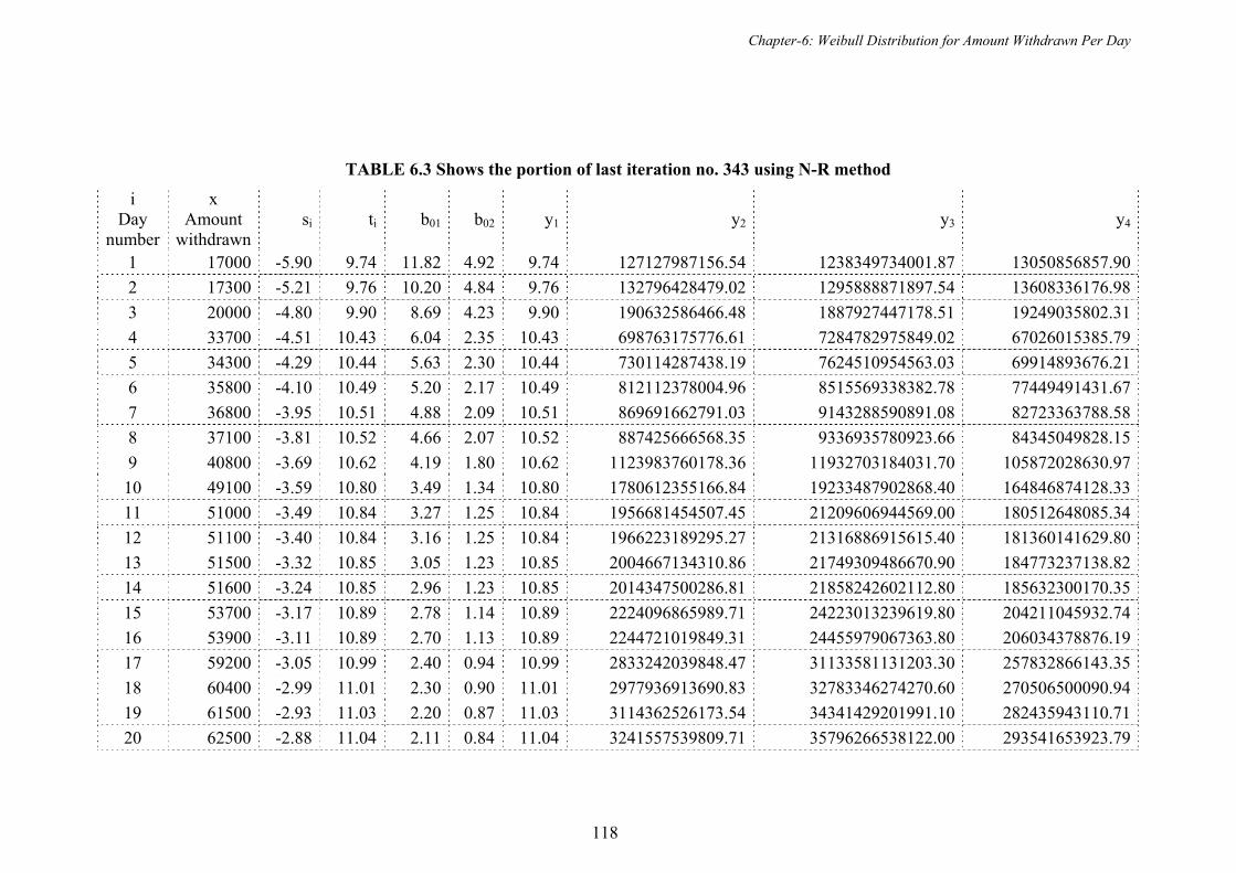
Chapter-6: Weibull Distribution for Amount Withdrawn Per Day
118
TABLE 6.3 Shows the portion of last iteration no. 343 using N-R method
i Day
number
x Amount
withdrawnsi ti b01 b02 y1 y2 y3 y4
1 17000 -5.90 9.74 11.82 4.92 9.74 127127987156.54 1238349734001.87 13050856857.90
2 17300 -5.21 9.76 10.20 4.84 9.76 132796428479.02 1295888871897.54 13608336176.98
3 20000 -4.80 9.90 8.69 4.23 9.90 190632586466.48 1887927447178.51 19249035802.31
4 33700 -4.51 10.43 6.04 2.35 10.43 698763175776.61 7284782975849.02 67026015385.79
5 34300 -4.29 10.44 5.63 2.30 10.44 730114287438.19 7624510954563.03 69914893676.21
6 35800 -4.10 10.49 5.20 2.17 10.49 812112378004.96 8515569338382.78 77449491431.67
7 36800 -3.95 10.51 4.88 2.09 10.51 869691662791.03 9143288590891.08 82723363788.58
8 37100 -3.81 10.52 4.66 2.07 10.52 887425666568.35 9336935780923.66 84345049828.15
9 40800 -3.69 10.62 4.19 1.80 10.62 1123983760178.36 11932703184031.70 105872028630.97
10 49100 -3.59 10.80 3.49 1.34 10.80 1780612355166.84 19233487902868.40 164846874128.33
11 51000 -3.49 10.84 3.27 1.25 10.84 1956681454507.45 21209606944569.00 180512648085.34
12 51100 -3.40 10.84 3.16 1.25 10.84 1966223189295.27 21316886915615.40 181360141629.80
13 51500 -3.32 10.85 3.05 1.23 10.85 2004667134310.86 21749309486670.90 184773237138.82
14 51600 -3.24 10.85 2.96 1.23 10.85 2014347500286.81 21858242602112.80 185632300170.35
15 53700 -3.17 10.89 2.78 1.14 10.89 2224096865989.71 24223013239619.80 204211045932.74
16 53900 -3.11 10.89 2.70 1.13 10.89 2244721019849.31 24455979067363.80 206034378876.19
17 59200 -3.05 10.99 2.40 0.94 10.99 2833242039848.47 31133581131203.30 257832866143.35
18 60400 -2.99 11.01 2.30 0.90 11.01 2977936913690.83 32783346274270.60 270506500090.94
19 61500 -2.93 11.03 2.20 0.87 11.03 3114362526173.54 34341429201991.10 282435943110.71
20 62500 -2.88 11.04 2.11 0.84 11.04 3241557539809.71 35796266538122.00 293541653923.79
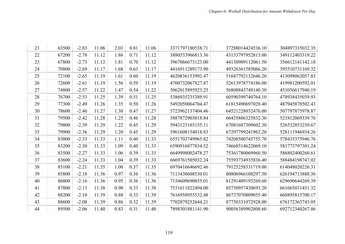
Chapter-6: Weibull Distribution for Amount Withdrawn Per Day
119
21 63500 -2.83 11.06 2.03 0.81 11.06 3371797180538.71 37288014424536.10 304897335032.35
22 67200 -2.78 11.12 1.86 0.71 11.12 3880533966813.36 43133797952813.00 349112403319.22
23 67800 -2.73 11.12 1.81 0.70 11.12 3967066673123.00 44130909112061.50 356612141142.18
24 70800 -2.69 11.17 1.68 0.63 11.17 4416911289173.90 49326361585066.20 395510731169.32
25 72100 -2.65 11.19 1.61 0.60 11.19 4620836153992.47 51687792132646.20 413098062057.83
26 72600 -2.61 11.19 1.56 0.59 11.19 4700732067827.87 52613978774186.00 419981200592.01
27 74800 -2.57 11.22 1.47 0.54 11.22 5062015895923.25 56808843749140.30 451056617940.19
28 76700 -2.53 11.25 1.39 0.51 11.25 5386935235389.91 60590399740764.10 478938435039.93
29 77300 -2.49 11.26 1.35 0.50 11.26 5492050064704.47 61815490697028.40 487945878502.43
30 78600 -2.46 11.27 1.30 0.47 11.27 5723962137404.46 64521228032476.00 507797875978.87
31 79500 -2.42 11.28 1.25 0.46 11.28 5887872903018.84 66435886325832.30 521812069339.76
32 79800 -2.39 11.29 1.22 0.45 11.29 5943123103155.11 67081687309602.30 526532853239.67
33 79900 -2.36 11.29 1.20 0.45 11.29 5961608154018.83 67297799241962.20 528111946934.26
34 83000 -2.33 11.33 1.11 0.40 11.33 6551703749965.82 74208500745755.70 578435375946.76
35 83200 -2.30 11.33 1.09 0.40 11.33 6590916877834.52 74668514622069.10 581773797301.24
36 83500 -2.27 11.33 1.06 0.39 11.33 6649998002478.27 75361780069960.50 586802400260.61
37 83600 -2.24 11.33 1.04 0.39 11.33 6669761505032.24 75593734935836.40 588484198747.02
38 85100 -2.21 11.35 1.00 0.37 11.35 6970416646692.46 79125258331719.00 614048020226.31
39 85800 -2.18 11.36 0.97 0.36 11.36 7113430608530.01 80806966108297.50 626194713888.36
40 86000 -2.16 11.36 0.95 0.36 11.36 7154609690855.01 81291409193269.60 629690644269.39
41 87800 -2.13 11.38 0.90 0.33 11.38 7531611822494.00 85730957430693.20 661665031451.32
42 88200 -2.10 11.39 0.88 0.33 11.39 7616958955532.48 86737070809055.40 668895815700.17
43 88600 -2.08 11.39 0.86 0.32 11.39 7702879252644.21 87750331072928.00 676172363743.05
44 89500 -2.06 11.40 0.83 0.31 11.40 7898301881141.90 90056389902808.60 692712340267.86
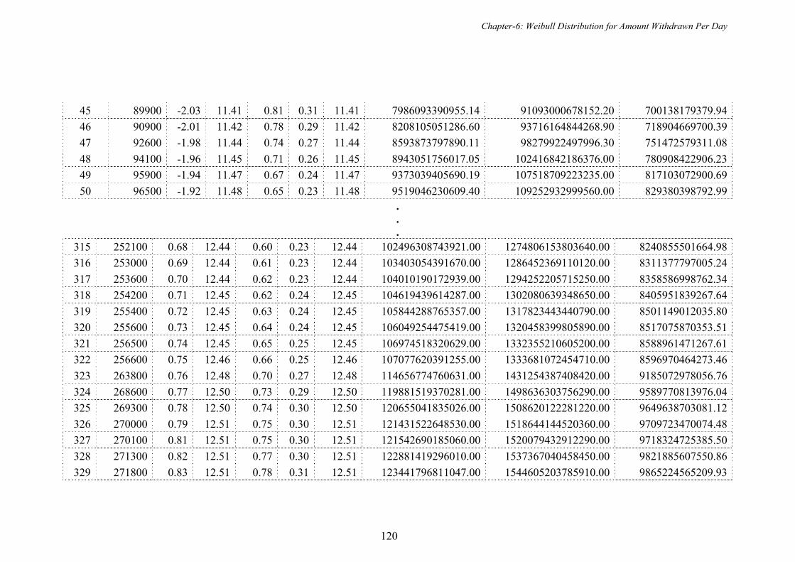
Chapter-6: Weibull Distribution for Amount Withdrawn Per Day
120
45 89900 -2.03 11.41 0.81 0.31 11.41 7986093390955.14 91093000678152.20 700138179379.94
46 90900 -2.01 11.42 0.78 0.29 11.42 8208105051286.60 93716164844268.90 718904669700.39
47 92600 -1.98 11.44 0.74 0.27 11.44 8593873797890.11 98279922497996.30 751472579311.08
48 94100 -1.96 11.45 0.71 0.26 11.45 8943051756017.05 102416842186376.00 780908422906.23
49 95900 -1.94 11.47 0.67 0.24 11.47 9373039405690.19 107518709223235.00 817103072900.69
50 96500 -1.92 11.48 0.65 0.23 11.48 9519046230609.40 109252932999560.00 829380398792.99 . . .
315 252100 0.68 12.44 0.60 0.23 12.44 102496308743921.00 1274806153803640.00 8240855501664.98
316 253000 0.69 12.44 0.61 0.23 12.44 103403054391670.00 1286452369110120.00 8311377797005.24
317 253600 0.70 12.44 0.62 0.23 12.44 104010190172939.00 1294252205715250.00 8358586998762.34
318 254200 0.71 12.45 0.62 0.24 12.45 104619439614287.00 1302080639348650.00 8405951839267.64
319 255400 0.72 12.45 0.63 0.24 12.45 105844288765357.00 1317823443440790.00 8501149012035.80
320 255600 0.73 12.45 0.64 0.24 12.45 106049254475419.00 1320458399805890.00 8517075870353.51
321 256500 0.74 12.45 0.65 0.25 12.45 106974518320629.00 1332355210605200.00 8588961471267.61
322 256600 0.75 12.46 0.66 0.25 12.46 107077620391255.00 1333681072454710.00 8596970464273.46
323 263800 0.76 12.48 0.70 0.27 12.48 114656774760631.00 1431254387408420.00 9185072978056.76
324 268600 0.77 12.50 0.73 0.29 12.50 119881519370281.00 1498636303756290.00 9589770813976.04
325 269300 0.78 12.50 0.74 0.30 12.50 120655041835026.00 1508620122281220.00 9649638703081.12
326 270000 0.79 12.51 0.75 0.30 12.51 121431522648530.00 1518644144520360.00 9709723470074.48
327 270100 0.81 12.51 0.75 0.30 12.51 121542690185060.00 1520079432912290.00 9718324725385.50
328 271300 0.82 12.51 0.77 0.30 12.51 122881419296010.00 1537367040458450.00 9821885607550.86
329 271800 0.83 12.51 0.78 0.31 12.51 123441796811047.00 1544605203785910.00 9865224565209.93
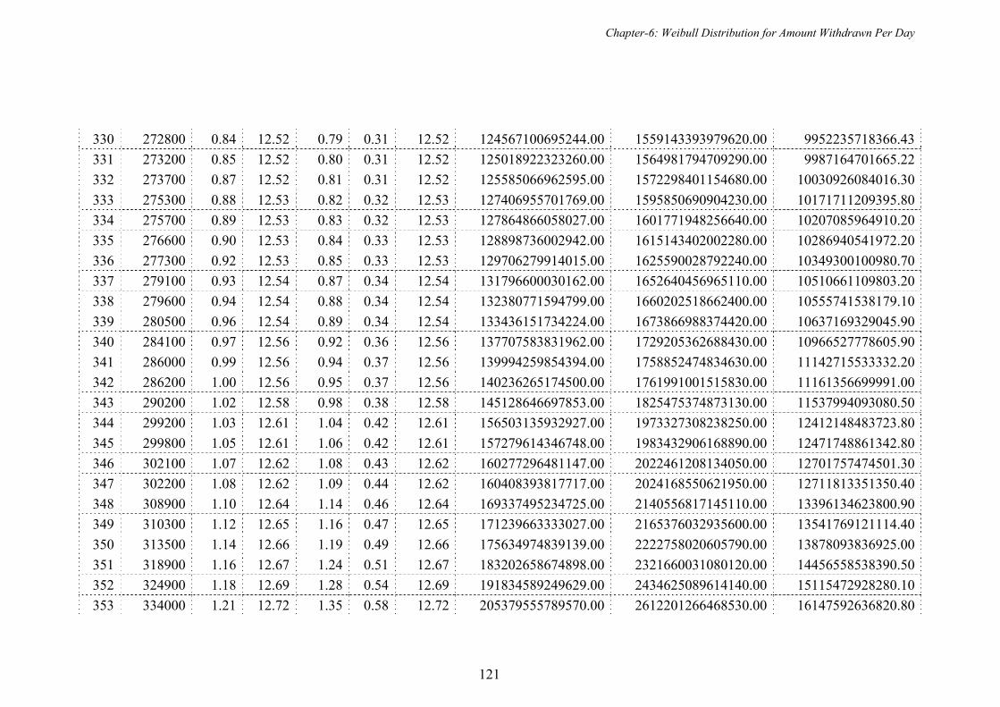
Chapter-6: Weibull Distribution for Amount Withdrawn Per Day
121
330 272800 0.84 12.52 0.79 0.31 12.52 124567100695244.00 1559143393979620.00 9952235718366.43
331 273200 0.85 12.52 0.80 0.31 12.52 125018922323260.00 1564981794709290.00 9987164701665.22
332 273700 0.87 12.52 0.81 0.31 12.52 125585066962595.00 1572298401154680.00 10030926084016.30
333 275300 0.88 12.53 0.82 0.32 12.53 127406955701769.00 1595850690904230.00 10171711209395.80
334 275700 0.89 12.53 0.83 0.32 12.53 127864866058027.00 1601771948256640.00 10207085964910.20
335 276600 0.90 12.53 0.84 0.33 12.53 128898736002942.00 1615143402002280.00 10286940541972.20
336 277300 0.92 12.53 0.85 0.33 12.53 129706279914015.00 1625590028792240.00 10349300100980.70
337 279100 0.93 12.54 0.87 0.34 12.54 131796600030162.00 1652640456965110.00 10510661109803.20
338 279600 0.94 12.54 0.88 0.34 12.54 132380771594799.00 1660202518662400.00 10555741538179.10
339 280500 0.96 12.54 0.89 0.34 12.54 133436151734224.00 1673866988374420.00 10637169329045.90
340 284100 0.97 12.56 0.92 0.36 12.56 137707583831962.00 1729205362688430.00 10966527778605.90
341 286000 0.99 12.56 0.94 0.37 12.56 139994259854394.00 1758852474834630.00 11142715533332.20
342 286200 1.00 12.56 0.95 0.37 12.56 140236265174500.00 1761991001515830.00 11161356699991.00
343 290200 1.02 12.58 0.98 0.38 12.58 145128646697853.00 1825475374873130.00 11537994093080.50
344 299200 1.03 12.61 1.04 0.42 12.61 156503135932927.00 1973327308238250.00 12412148483723.80
345 299800 1.05 12.61 1.06 0.42 12.61 157279614346748.00 1983432906168890.00 12471748861342.80
346 302100 1.07 12.62 1.08 0.43 12.62 160277296481147.00 2022461208134050.00 12701757474501.30
347 302200 1.08 12.62 1.09 0.44 12.62 160408393817717.00 2024168550621950.00 12711813351350.40
348 308900 1.10 12.64 1.14 0.46 12.64 169337495234725.00 2140556817145110.00 13396134623800.90
349 310300 1.12 12.65 1.16 0.47 12.65 171239663333027.00 2165376032935600.00 13541769121114.40
350 313500 1.14 12.66 1.19 0.49 12.66 175634974839139.00 2222758020605790.00 13878093836925.00
351 318900 1.16 12.67 1.24 0.51 12.67 183202658674898.00 2321660031080120.00 14456558538390.50
352 324900 1.18 12.69 1.28 0.54 12.69 191834589249629.00 2434625089614140.00 15115472928280.10
353 334000 1.21 12.72 1.35 0.58 12.72 205379555789570.00 2612201266468530.00 16147592636820.80

Chapter-6: Weibull Distribution for Amount Withdrawn Per Day
122
354 335400 1.23 12.72 1.38 0.58 12.72 207512257967221.00 2640194878223940.00 16309908621450.60
355 346000 1.25 12.75 1.45 0.63 12.75 224086791631580.00 2858046425416370.00 17569655180258.20
356 349000 1.28 12.76 1.49 0.65 12.76 228915570867255.00 2921609874639300.00 17936117700160.40
357 369400 1.31 12.82 1.62 0.74 12.82 263388794701368.00 3376548302490820.00 20545732197304.40
358 373100 1.34 12.83 1.66 0.76 12.83 269950759046908.00 3463360733168090.00 21041242285882.70
359 380730 1.38 12.85 1.73 0.79 12.85 283786626386432.00 3646614372558490.00 22084827483222.00
360 382900 1.41 12.86 1.78 0.80 12.86 287796803921466.00 3699780198481830.00 22387005687905.00
361 440900 1.46 13.00 2.10 1.08 13.00 407656284471763.00 5298134811427580.00 31366443509682.00
362 446300 1.51 13.01 2.18 1.10 13.01 420089899076765.00 5464843067573050.00 32292880348840.40
363 457300 1.57 13.03 2.30 1.15 13.03 446107080456430.00 5814155919453810.00 34228790901097.00
364 488700 1.65 13.10 2.53 1.30 13.10 525544997669219.00 6884378842903880.00 40119457525181.40
365 523100 1.78 13.17 2.84 1.46 13.17 621583635473986.00 8184719880536030.00 47205795864543.80
TOT 63822850 -208.4 4365.0 232.58 95.28 4365.05 20913184615845900.00 259418951595684000.00 1687553151508530.00
-0.57 11.96 Remark: As total numbers of iterations are 343, we did not show all iterations because of space. If any one require we can provide it as we
have stored as soft copy.
b0 b1
( ) Difference (b1-b0)
t1
( ) 2.3911503 2.3910504 0.0000999 4623433291804.207140

Chapter-6: Weibull Distribution for Amount Withdrawn Per Day
123
Thus, using N-R method =2.3910504
We obtain (uncensored) as =nxi
, on putting value of we get
=4623433291804.207140.
6.6 FINAL SOLUTION USING GOAL-SEEK FACILITY OF EXCEL
For the estimation of parameters, as we know,
n
ixnnL1
ln1lnlnln
2
1ln
n
ixnL
n
iin
i
xxxnL 1
1
lnln
ln
And MLE’s and are solutions of
n
in
i
n
ii
xnx
xx
1
1
ˆ
1
ˆ
ln1
ˆ1
ln
=365
44365.04541=11.95902853 (6.13)
Here, value on the left hand side of the equation is depending on the value of . Goal
seek facility of Excel is useful to find the value of by iterative method in such a
way that left hand side of the equation is equal to right hand side (11.95902853).
Goal-Seek facility of Excel
The basic forecasting command in Excel is Goal Seek, which is located on the Tools
menu. The Goal Seek command determines the unknown value that produces a
desired result of equation (6.13).
Goal Seek is simple; it can calculate only one unknown value.
To use Goal Seek, set up the worksheet which contains the following:
Chapter-6: Weibull Distribution for Amount Withdrawn Per Day
124
1. A formula that calculates your goal (for example, a formula that mentioned in
equation-(6.13))
2. An empty variable cell for the unknown number that will produce the desired
outcome (for example, a cell to hold the value of )
3. Values in any cells (other than the empty cell) that the formula refers to (for
example, a cell that helps to evaluate the formula)
The empty cell should be referenced in your formula; it serves as the variable that
Excel changes.
When the Goal Seek command starts to run, it repeatedly tries new values in the
variable cell to find a solution to the problem we have set. This process is called
iteration, and it continues until Excel has run the problem 100 times or has found an
answer within .001 of the target value you specified. (We can adjust these iteration
settings by clicking Options on the Tools menu, and then adjusting the Iteration
options on the Calculations tab.) Here we have set maximum iterations 1000 and
maximum change 0.0001. Because it calculates so fast, the Goal Seek command can
save our significant time. To forecast using the Goal Seek command we have the
following algorithm for (6.13):
1. Create a worksheet that contains clumns of i (serial number of the day), xi
(amount withdrawn per day) and ln xi.
2. Keep one cell for the variable with any initial value.
3. To calculate the left had side of the equation (6.13), add two more columns of
ix and ixix ln using the initial value of the variable.
4. The formula cell determines the value in the variable cell by following way.
4.1 In your worksheet, select the cell containing the formula. (i.e. formula
given in L.H.S. of equation (6.13))
4.2 On the Tools menu, click Goal Seek and the Goal Seek dialog box
opens.
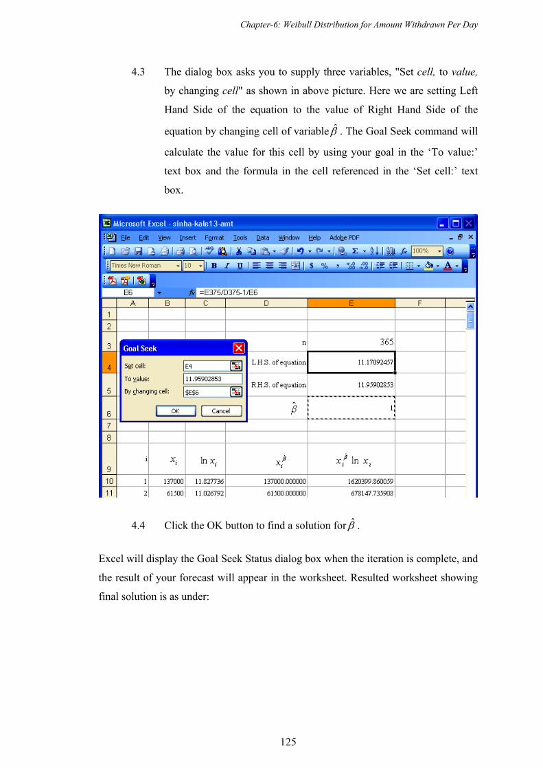
Chapter-6: Weibull Distribution for Amount Withdrawn Per Day
125
4.3 The dialog box asks you to supply three variables, "Set cell, to value,
by changing cell" as shown in above picture. Here we are setting Left
Hand Side of the equation to the value of Right Hand Side of the
equation by changing cell of variable . The Goal Seek command will
calculate the value for this cell by using your goal in the ‘To value:’
text box and the formula in the cell referenced in the ‘Set cell:’ text
box.
4.4 Click the OK button to find a solution for .
Excel will display the Goal Seek Status dialog box when the iteration is complete, and
the result of your forecast will appear in the worksheet. Resulted worksheet showing
final solution is as under:

Chapter-6: Weibull Distribution for Amount Withdrawn Per Day
126
TABLE 6.4 Final solution of and using goal seek of Excel
n 365
L.H.S. of equation 11.95910706
R.H.S. of equation 11.95902853
2.344353817
i Day
number
xi Amount
withdrawn 1 137000 11.827736 1102276296477.690000 13037433259553.400000
2 61500 11.026792 168584505629.394000 1858946354500.900000
3 123900 11.727230 870885695573.228000 10213076914584.100000
4 196300 12.187399 2561402961634.430000 31216840867231.300000
5 140100 11.850112 1161640877782.790000 13765574194562.300000
6 152100 11.932293 1408459628465.180000 16806153639109.800000
7 109100 11.600020 646314178458.130000 7497257507448.330000
8 201200 12.212055 2713816572704.080000 33141276478327.400000
9 77300 11.255449 288152408967.913000 3243284810958.980000
10 107000 11.580584 617525727915.382000 7151308634339.850000
11 143000 11.870600 1218797956106.680000 14467862907144.400000
12 151400 11.927681 1393310364972.950000 16618961037912.700000
13 195000 12.180755 2521812732407.910000 30717582639662.400000
14 35800 10.485703 47414705299.444700 497176525776.267000
15 117500 11.674194 769064252127.986000 8978204979845.650000
16 17000 9.740969 8273115288.009010 80588156435.274700
17 183100 12.117788 2175722522903.350000 26364943693364.600000
18 108100 11.590812 632511578058.684000 7331322791395.840000
19 103500 11.547327 571208354707.685000 6595929595072.660000
20 95900 11.471061 477689249197.555000 5479602641204.880000
21 53700 10.891168 122668561061.524000 1336003941247.470000
22 101300 11.525842 543149781978.534000 6260258401171.200000
23 37100 10.521372 51550058945.522200 542377359602.881000
24 137400 11.830652 1109836001132.560000 13130083127762.000000
25 183700 12.121059 2192473705733.660000 26575103737752.300000
26 108400 11.593583 636634421532.110000 7380874240963.130000
27 158900 11.976030 1560539123104.560000 18689063904602.700000
28 106000 11.571194 604080736464.402000 6989935618671.490000
29 163600 12.005180 1670908924762.960000 20059561909377.800000
30 53900 10.894886 123742299445.066000 1348158215749.750000
31 256500 12.454884 4795287176125.570000 59724745254843.500000
ix ii xx ln
ixln
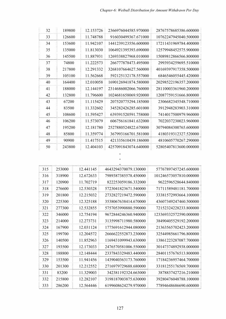
Chapter-6: Weibull Distribution for Amount Withdrawn Per Day
127
32 189800 12.153726 2366976044585.970000 28767578685386.600000
33 126600 11.748788 916030499367.671000 10762247945040.500000
34 153600 11.942107 1441239123556.600000 17211431969784.400000
35 135000 11.813030 1064921395393.690000 12579948452575.900000
36 145500 11.887931 1269338827968.010000 15089812866566.800000
37 74800 11.222573 266777878473.495000 2993934259695.510000
38 217800 12.291332 3268107664627.560000 40169397917358.500000
39 105100 11.562668 592125132178.557000 6846546055445.420000
40 164400 12.010058 1690126941874.580000 20298522196357.200000
41 188000 12.144197 2314686002066.760000 28110003361960.200000
42 132800 11.796600 1024681658069.920000 12087759151666.800000
43 67200 11.115429 207520775294.185000 2306682345548.710000
44 83500 11.332602 345282426285.601000 3912948283903.310000
45 108600 11.595427 639391520591.758000 7414017500979.960000
46 106200 11.573079 606756161841.632000 7022037230023.960000
47 195200 12.181780 2527880524822.670000 30794084300765.600000
48 85800 11.359774 367993166701.581000 4180319312327.520000
49 90900 11.417515 421335610439.186000 4810605770267.290000
50 243800 12.404103 4257091843074.640000 52805407813600.000000
.
.
. 315 253000 12.441145 4643294370079.130000 57767897457245.600000
316 318900 12.672633 7989387385578.450000 101246573057810.000000
317 120900 11.702719 822253059186.332000 9622596528644.840000
318 276600 12.530328 5723041823671.540000 71711589481181.700000
319 201800 12.215032 2732827219472.590000 33381572993664.100000
320 225300 12.325188 3538067638414.670000 43607349247460.500000
321 277300 12.532855 5757053990880.590000 72152324228233.800000
322 346000 12.754194 9672844246360.940000 123369332572590.000000
323 214000 12.273731 3135998711980.580000 38490405529192.200000
324 167900 12.031124 1775691612944.080000 21363565702423.200000
325 199700 12.204572 2666622552873.230000 32544985661796.800000
326 140500 11.852963 1169431099943.630000 13861223287087.700000
327 193500 12.173033 2476570581006.550000 30147374892938.000000
328 188800 12.148444 2337843329483.440000 28401157676513.800000
329 153500 11.941456 1439040363173.760000 17184236957464.700000
330 201300 12.212552 2716979729688.680000 33181255176569.700000
331 83200 11.329003 342381192324.663000 3878837427216.210000
332 215800 12.282107 3198187003875.630000 39280476048788.100000
333 286200 12.564446 6199608624279.970000 77894648686690.600000
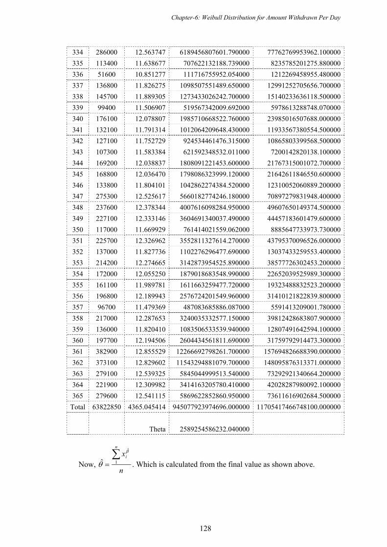
Chapter-6: Weibull Distribution for Amount Withdrawn Per Day
128
334 286000 12.563747 6189456807601.790000 77762769953962.100000
335 113400 11.638677 707622132188.739000 8235785201275.880000
336 51600 10.851277 111716755952.054000 1212269458955.480000
337 136800 11.826275 1098507551489.650000 12991252705656.700000
338 145700 11.889305 1273433026242.700000 15140233636118.500000
339 99400 11.506907 519567342009.692000 5978613288748.070000
340 176100 12.078807 1985710668522.760000 23985016507688.000000
341 132100 11.791314 1012064209648.430000 11933567380554.500000
342 127100 11.752729 924534461476.315000 10865803399568.500000
343 107300 11.583384 621592348532.011000 7200142820138.100000
344 169200 12.038837 1808091221453.600000 21767315001072.700000
345 168800 12.036470 1798086323999.120000 21642611846550.600000
346 133800 11.804101 1042862274384.520000 12310052060889.200000
347 275300 12.525617 5660182774246.180000 70897279831948.400000
348 237600 12.378344 4007616098284.950000 49607650149374.500000
349 227100 12.333146 3604691340037.490000 44457183601479.600000
350 117000 11.669929 761414021559.062000 8885647733973.730000
351 225700 12.326962 3552811327614.270000 43795370096526.000000
352 137000 11.827736 1102276296477.690000 13037433259553.400000
353 214200 12.274665 3142873954525.890000 38577726302453.200000
354 172000 12.055250 1879018683548.990000 22652039525989.300000
355 161100 11.989781 1611663259477.720000 19323488832523.200000
356 196800 12.189943 2576724201549.960000 31410121822839.800000
357 96700 11.479369 487083685886.087000 5591413209001.780000
358 217000 12.287653 3240035332577.150000 39812428683807.900000
359 136000 11.820410 1083506533539.940000 12807491642594.100000
360 197700 12.194506 2604434561811.690000 31759792914473.300000
361 382900 12.855529 12266692798261.700000 157694826688390.000000
362 373100 12.829602 11543294881079.700000 148095876313371.000000
363 279100 12.539325 5845044999513.540000 73292921340664.200000
364 221900 12.309982 3414163205780.410000 42028287980092.100000
365 279600 12.541115 5869622852860.950000 73611616902684.500000
Total 63822850 4365.045414 945077923974696.000000 11705417466748100.000000
Theta 2589254586232.040000
Now, n
xn
i 1
ˆ
ˆ
. Which is calculated from the final value as shown above.

Chapter-6: Weibull Distribution for Amount Withdrawn Per Day
129
365
0074696.00009450779239 = 2589254586232.040000
TABLE 6.5 Final solutions using all the methods
Method of calculation Graphical Newton-Raphson Goal Seek of Excel 2.4410138 2.3910504 2.344353817
8578516936201.362400 4623433291804.207140 2589254586232.040000
6.7 GOODNESS OF FIT TEST
Using Excel we have prepared a worksheet ‘goodness-amt.xls’ having columns like x
and f(x) for unique values of x with the help of =2.3910504 and
=4623433291804.207140 (obtained using N-R method).
Where
xxxf exp,, 1
x
exF
1)(
a
b
aFbFdxxf )()()(
=
ˆˆ ba
ee
And
i
ii
EEO 2
2
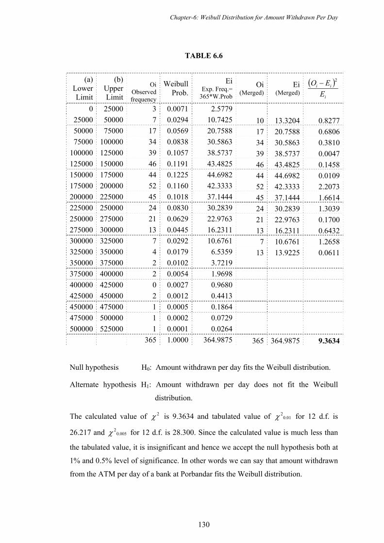
Chapter-6: Weibull Distribution for Amount Withdrawn Per Day
130
TABLE 6.6
(a) Lower Limit
(b) Upper Limit
Oi
Observed frequency
Weibull Prob.
EiExp. Freq.=
365*W.Prob
Oi(Merged)
Ei (Merged)
i
ii
EEO 2
0 25000 3 0.0071 2.5779 25000 50000 7 0.0294 10.7425 10 13.3204 0.827750000 75000 17 0.0569 20.7588 17 20.7588 0.680675000 100000 34 0.0838 30.5863 34 30.5863 0.3810
100000 125000 39 0.1057 38.5737 39 38.5737 0.0047125000 150000 46 0.1191 43.4825 46 43.4825 0.1458150000 175000 44 0.1225 44.6982 44 44.6982 0.0109175000 200000 52 0.1160 42.3333 52 42.3333 2.2073200000 225000 45 0.1018 37.1444 45 37.1444 1.6614225000 250000 24 0.0830 30.2839 24 30.2839 1.3039250000 275000 21 0.0629 22.9763 21 22.9763 0.1700275000 300000 13 0.0445 16.2311 13 16.2311 0.6432300000 325000 7 0.0292 10.6761 7 10.6761 1.2658325000 350000 4 0.0179 6.5359 13 13.9225 0.0611350000 375000 2 0.0102 3.7219 375000 400000 2 0.0054 1.9698 400000 425000 0 0.0027 0.9680 425000 450000 2 0.0012 0.4413 450000 475000 1 0.0005 0.1864 475000 500000 1 0.0002 0.0729 500000 525000 1 0.0001 0.0264 365 1.0000 364.9875 365 364.9875 9.3634
Null hypothesis H0: Amount withdrawn per day fits the Weibull distribution.
Alternate hypothesis H1: Amount withdrawn per day does not fit the Weibull
distribution.
The calculated value of 2 is 9.3634 and tabulated value of 01.02 for 12 d.f. is
26.217 and 005.02 for 12 d.f. is 28.300. Since the calculated value is much less than
the tabulated value, it is insignificant and hence we accept the null hypothesis both at
1% and 0.5% level of significance. In other words we can say that amount withdrawn
from the ATM per day of a bank at Porbandar fits the Weibull distribution.

Chapter-6: Weibull Distribution for Amount Withdrawn Per Day
131
6.8 MEAN AND VARIANCE
Now we find expected mean and variance of Weibull distribution with the help of
‘mean-weibull.xls’ file of Excel, for the following value of and (obtained from
different methods)
Graphical 2.4410138 8578516936201.360N-R 2.3910504 4623433291804.200Goal Seek 2.344535817 2589254586232.040
Mean:
Here mean is obtained using the formula
1
1
1 for the different methods
as:
TABLE 6.7
Method 1
1
1
Mean
Graphical 198782.13165 1.409665853 0.8867799 176275.993487N-R 198070.78600 1.418226232 0.8864218 175574.256652Goal Seek 197021.10056 1.426523661 0.8861373 174587.737295
Variance:
Similarly variance is obtained using the formula
12 2
2
2 for
different methods as:
TABLE 6.8
Method 2
2
1
2
12
Variance Graphical 39514335863 1.81933 1.40966 0.93665 0.78637 5938179522N-R 39232036266 1.83645 1.41822 0.94156 0.78574 6113271086Goal Seek 38817314067 1.85304 1.42652 0.94654 0.78523 6261274822
Chapter-6: Weibull Distribution for Amount Withdrawn Per Day
132
Conclusion: From all the three methods, we concluded that withrawl of average
amount per day is more or less same. We also found from the observed amount
withdrawn per day with the help of available data, that the average withdrawn amount
is Rs.173017 only.
Finally we conclude that the Bank must keep more than Rs.176275 per day at the
ATM so that customer will not return without withdrawing money. However during
the festival period, Bank must keep more amount which must be equal to its mode
amount.

References
133
References
1. http://www.en.wikipedia.org/wiki/Time_series
2. Ajay Goel & Alka Goel, Mathematics and Statistics, Taxmann Allied Services
Pvt. Ltd., 879-929
3. http://www.ecompare.co.in, Loans, Home Loans & Rates, Personal Loans,
Credit Cards in India
4. http://www.ecompare.co.in/savings/, Fixed Deposits, Interest Rates ...
5. http://www.rbi.org.in/, Reserve Bank of India
6. http://www.en.wikipedia.org/wiki/Deposit_account
7. http://www.allbankingsolutions.com/dep1.htm, Saving, Recurring, Term,
Fixed Deposits in Banks in India. Tips ...
8. http://www.en.wikipedia.org/wiki/Weibull_distribution
9. Johnson and Kotz, Continuous univariate distributions-1, John Wiley & Sons,
250-267
10. Sinha & Kale, Life Testing and Reliability Estimation, Wiley Eastern Limited,
41-45
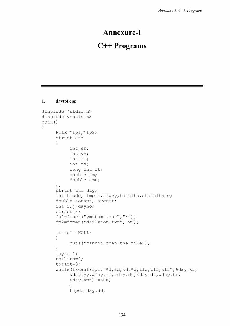
Annexure-I: C++ Programs
134
Annexure-I
C++ Programs
1. daytot.cpp #include <stdio.h> #include <conio.h> main() { FILE *fp1,*fp2; struct atm { int sr; int yy; int mm; int dd; long int dt; double tm; double amt; }; struct atm day; int tmpdd, tmpmm,tmpyy,tothits,gtothits=0; double totamt, avgamt; int i,j,dayno; clrscr(); fp1=fopen("ymdtamt.csv","r"); fp2=fopen("dailytot.txt","w"); if(fp1==NULL) { puts("cannot open the file"); } dayno=1; tothits=0; totamt=0; while(fscanf(fp1,"%d,%d,%d,%d,%ld,%lf,%lf",&day.sr,
&day.yy,&day.mm,&day.dd,&day.dt,&day.tm, &day.amt)!=EOF)
{ tmpdd=day.dd;
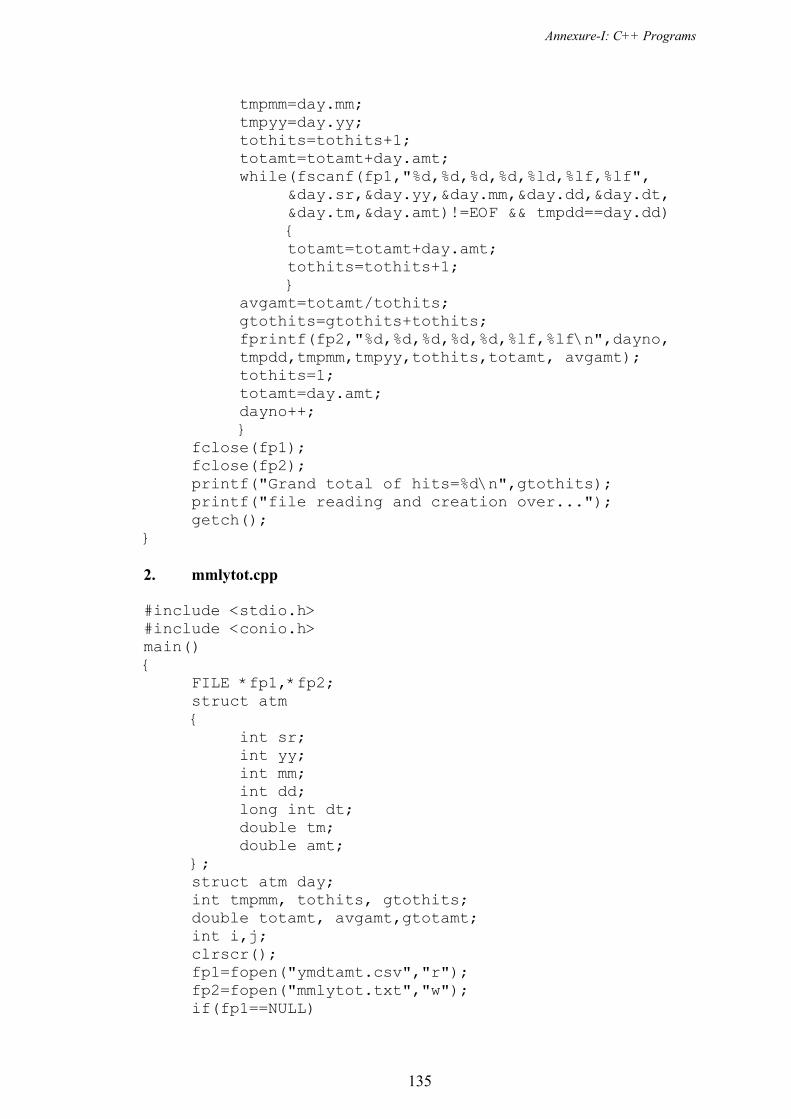
Annexure-I: C++ Programs
135
tmpmm=day.mm; tmpyy=day.yy; tothits=tothits+1; totamt=totamt+day.amt; while(fscanf(fp1,"%d,%d,%d,%d,%ld,%lf,%lf",
&day.sr,&day.yy,&day.mm,&day.dd,&day.dt, &day.tm,&day.amt)!=EOF && tmpdd==day.dd)
{ totamt=totamt+day.amt; tothits=tothits+1; } avgamt=totamt/tothits; gtothits=gtothits+tothits; fprintf(fp2,"%d,%d,%d,%d,%d,%lf,%lf\n",dayno,
tmpdd,tmpmm,tmpyy,tothits,totamt, avgamt); tothits=1; totamt=day.amt; dayno++; } fclose(fp1); fclose(fp2); printf("Grand total of hits=%d\n",gtothits); printf("file reading and creation over..."); getch(); } 2. mmlytot.cpp #include <stdio.h> #include <conio.h> main() { FILE *fp1,*fp2; struct atm { int sr; int yy; int mm; int dd; long int dt; double tm; double amt; }; struct atm day; int tmpmm, tothits, gtothits; double totamt, avgamt,gtotamt; int i,j; clrscr(); fp1=fopen("ymdtamt.csv","r"); fp2=fopen("mmlytot.txt","w"); if(fp1==NULL)

Annexure-I: C++ Programs
136
{ puts("cannot open the file"); } printf("\n\n --------------------------------------- ------\n"); printf(" Month Total no. Total
Average\n"); printf(" Number of hits Amount(Rs.) Amount(Rs.)\n"); printf(" ------------------------------------------- ------\n"); tothits=0; totamt=0; gtothits=0; gtotamt=0; while(fscanf(fp1,"%d,%d,%d,%d,%ld,%lf,%lf",&day.sr,
&day.yy,&day.mm,&day.dd,&day.dt,&day.tm, &day.amt)!=EOF)
{ tmpmm=day.mm; tothits=tothits+1; totamt=totamt+day.amt; while(fscanf(fp1,"%d,%d,%d,%d,%ld,%lf,%lf",
&day.sr,&day.yy,&day.mm,&day.dd,&day.dt, &day.tm,&day.amt)!=EOF && tmpmm==day.mm)
{ totamt=totamt+day.amt; tothits=tothits+1; } avgamt=totamt/tothits; gtothits=gtothits+tothits; gtotamt=gtotamt+totamt; fprintf(fp2,"\n%d,%d,%lf,%lf",tmpmm,tothits, totamt, avgamt); printf("\n %2d %7d 12.2lf%11.2lf",tmpmm,
tothits, totamt, avgamt); tothits=1; totamt=day.amt; } printf("\n ----------------------------------------- ----\n"); printf(" %7d %12.2lf\n",
gtothits,gtotamt); printf(" ------------------------------------------- --\n"); fclose(fp1); fclose(fp2); printf(" file reading and creation over..."); getch(); }

Annexure-I: C++ Programs
137
3. qmahit.cpp #include <stdio.h> # include <conio.h> main() { FILE *fp1,*fp2; struct atm { int mm; int tothits; double totamt; double avgamt; }; struct atm day; int mnth[13], hits[13], mtot3[13]={0}, i; float mavg3[13]; clrscr(); fp1=fopen("mmlytot.txt","r"); fp2=fopen("qmahit.txt","w"); if(fp1==NULL) { puts("cannot open the file"); } i=1; while(fscanf(fp1,"%d,%d,%lf,%lf",&day.mm,
&day.tothits,&day.totamt,&day.avgamt)!=EOF) { mnth[i]=day.mm; hits[i]=day.tothits; i++; } fclose(fp1); for(i=2;i<=11;i++) { mtot3[i]=hits[i-1]+hits[i]+hits[i+1]; mavg3[i]=mtot3[i]/3; } printf(" Quarterly moving average for
hits\n"); printf("--------------------------------------- -----\n"); printf(" Month Hits Quarterly
Quarterly\n"); printf("Number moving
moving\n"); printf(" total
average\n"); printf("--------------------------------------- -----\n"); for(i=1;i<=12;i++)

Annexure-I: C++ Programs
138
{ if(i==1||i==12) { printf(" %2d %5d %5d\n",mnth[i],hits[i],mtot3[i]); continue; } printf(" %2d %5d %5d %8.2f\n",
mnth[i],hits[i],mtot3[i],mavg3[i]); fprintf(fp2,"%2d,%8.2f\n",mnth[i],mavg3[i]); } printf("---------------------------------------\n"); fclose(fp2); getch(); } 4. qmaamt.cpp #include <stdio.h> # include <conio.h> main() { FILE *fp1,*fp2; struct atm { int mm; int tothits; double totamt; double avgamt; }; struct atm day; int mnth[13],i; double amt[13], mtot3[13]={0}, mavg3[13]={0}; clrscr(); fp1=fopen("mmlytot.txt","r"); fp2=fopen("qmaamt.txt","w"); if(fp1==NULL) { puts("cannot open the file"); } i=1; while(fscanf(fp1,"%d,%d,%lf,%lf",&day.mm,
&day.tothits,&day.totamt,&day.avgamt)!=EOF) { mnth[i]=day.mm; amt[i]=day.totamt; i++; } fclose(fp1); for(i=2;i<=11;i++) {
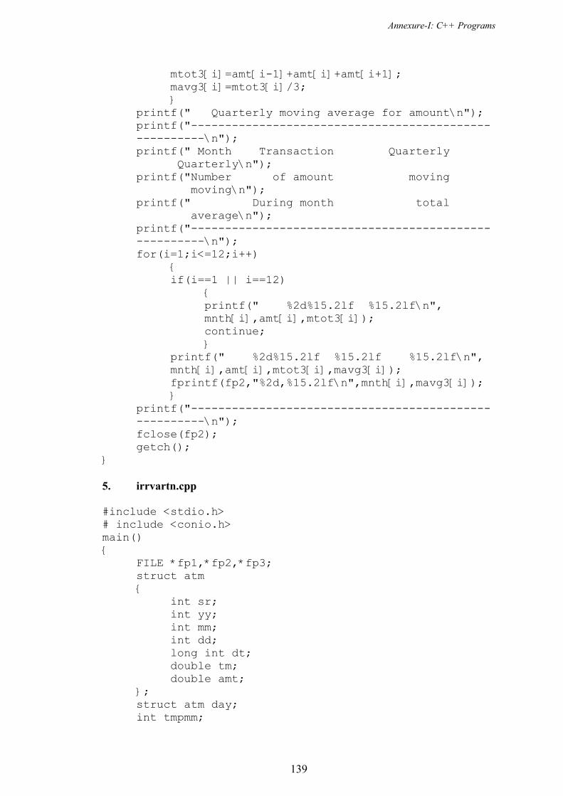
Annexure-I: C++ Programs
139
mtot3[i]=amt[i-1]+amt[i]+amt[i+1]; mavg3[i]=mtot3[i]/3; } printf(" Quarterly moving average for amount\n"); printf("-------------------------------------------- ----------\n"); printf(" Month Transaction Quarterly
Quarterly\n"); printf("Number of amount moving
moving\n"); printf(" During month total
average\n"); printf("-------------------------------------------- ----------\n"); for(i=1;i<=12;i++) { if(i==1 || i==12) { printf(" %2d%15.2lf %15.2lf\n", mnth[i],amt[i],mtot3[i]); continue; } printf(" %2d%15.2lf %15.2lf %15.2lf\n", mnth[i],amt[i],mtot3[i],mavg3[i]); fprintf(fp2,"%2d,%15.2lf\n",mnth[i],mavg3[i]); } printf("-------------------------------------------- ----------\n"); fclose(fp2); getch(); } 5. irrvartn.cpp #include <stdio.h> # include <conio.h> main() { FILE *fp1,*fp2,*fp3; struct atm { int sr; int yy; int mm; int dd; long int dt; double tm; double amt; }; struct atm day; int tmpmm;
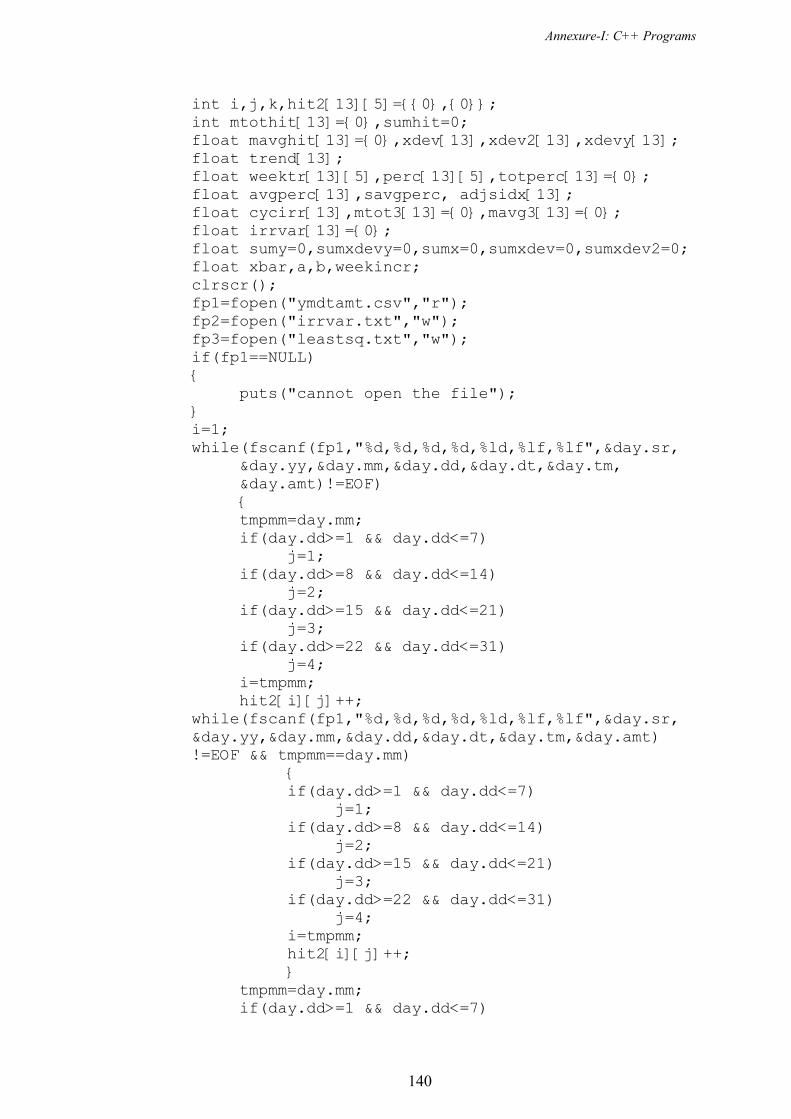
Annexure-I: C++ Programs
140
int i,j,k,hit2[13][5]={{0},{0}}; int mtothit[13]={0},sumhit=0;
float mavghit[13]={0},xdev[13],xdev2[13],xdevy[13]; float trend[13];
float weektr[13][5],perc[13][5],totperc[13]={0}; float avgperc[13],savgperc, adjsidx[13];
float cycirr[13],mtot3[13]={0},mavg3[13]={0}; float irrvar[13]={0};
float sumy=0,sumxdevy=0,sumx=0,sumxdev=0,sumxdev2=0; float xbar,a,b,weekincr;
clrscr(); fp1=fopen("ymdtamt.csv","r"); fp2=fopen("irrvar.txt","w"); fp3=fopen("leastsq.txt","w"); if(fp1==NULL) { puts("cannot open the file"); } i=1; while(fscanf(fp1,"%d,%d,%d,%d,%ld,%lf,%lf",&day.sr,
&day.yy,&day.mm,&day.dd,&day.dt,&day.tm, &day.amt)!=EOF)
{ tmpmm=day.mm; if(day.dd>=1 && day.dd<=7) j=1; if(day.dd>=8 && day.dd<=14) j=2; if(day.dd>=15 && day.dd<=21) j=3; if(day.dd>=22 && day.dd<=31) j=4; i=tmpmm; hit2[i][j]++; while(fscanf(fp1,"%d,%d,%d,%d,%ld,%lf,%lf",&day.sr,
&day.yy,&day.mm,&day.dd,&day.dt,&day.tm,&day.amt) !=EOF && tmpmm==day.mm)
{ if(day.dd>=1 && day.dd<=7) j=1; if(day.dd>=8 && day.dd<=14) j=2; if(day.dd>=15 && day.dd<=21) j=3; if(day.dd>=22 && day.dd<=31) j=4; i=tmpmm; hit2[i][j]++; } tmpmm=day.mm; if(day.dd>=1 && day.dd<=7)
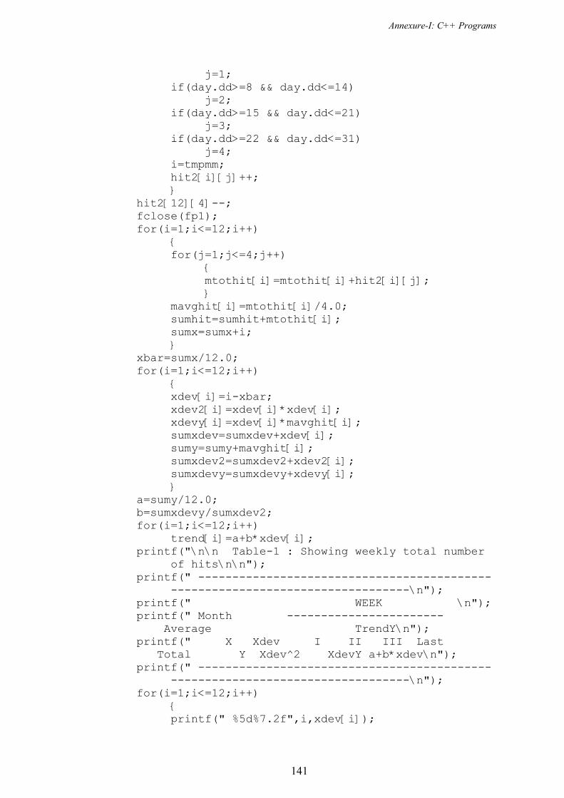
Annexure-I: C++ Programs
141
j=1; if(day.dd>=8 && day.dd<=14) j=2; if(day.dd>=15 && day.dd<=21) j=3; if(day.dd>=22 && day.dd<=31) j=4; i=tmpmm; hit2[i][j]++; } hit2[12][4]--; fclose(fp1); for(i=1;i<=12;i++) { for(j=1;j<=4;j++) { mtothit[i]=mtothit[i]+hit2[i][j]; } mavghit[i]=mtothit[i]/4.0; sumhit=sumhit+mtothit[i]; sumx=sumx+i; } xbar=sumx/12.0; for(i=1;i<=12;i++) { xdev[i]=i-xbar; xdev2[i]=xdev[i]*xdev[i]; xdevy[i]=xdev[i]*mavghit[i]; sumxdev=sumxdev+xdev[i]; sumy=sumy+mavghit[i]; sumxdev2=sumxdev2+xdev2[i]; sumxdevy=sumxdevy+xdevy[i]; } a=sumy/12.0; b=sumxdevy/sumxdev2; for(i=1;i<=12;i++) trend[i]=a+b*xdev[i]; printf("\n\n Table-1 : Showing weekly total number of hits\n\n"); printf(" ------------------------------------------- -----------------------------------\n"); printf(" WEEK \n"); printf(" Month ----------------------- Average TrendY\n"); printf(" X Xdev I II III Last
Total Y Xdev^2 XdevY a+b*xdev\n"); printf(" ------------------------------------------- -----------------------------------\n"); for(i=1;i<=12;i++) { printf(" %5d%7.2f",i,xdev[i]);
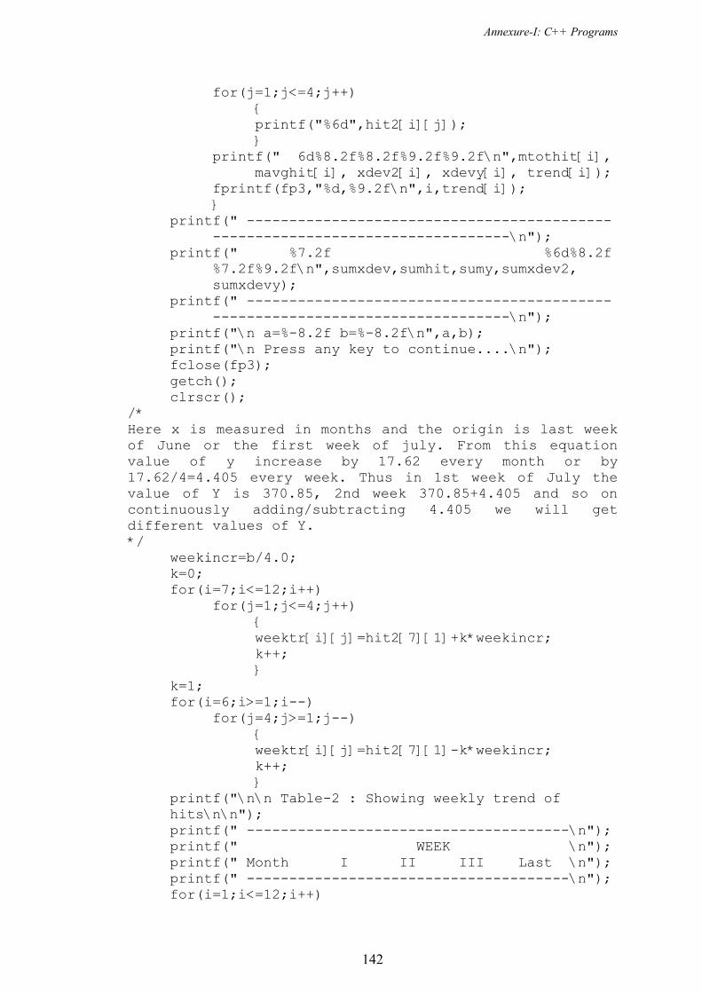
Annexure-I: C++ Programs
142
for(j=1;j<=4;j++) { printf("%6d",hit2[i][j]); } printf(" 6d%8.2f%8.2f%9.2f%9.2f\n",mtothit[i],
mavghit[i], xdev2[i], xdevy[i], trend[i]); fprintf(fp3,"%d,%9.2f\n",i,trend[i]); } printf(" ------------------------------------------- -----------------------------------\n"); printf(" %7.2f %6d%8.2f %7.2f%9.2f\n",sumxdev,sumhit,sumy,sumxdev2,
sumxdevy); printf(" ------------------------------------------- -----------------------------------\n"); printf("\n a=%-8.2f b=%-8.2f\n",a,b); printf("\n Press any key to continue....\n"); fclose(fp3); getch(); clrscr(); /* Here x is measured in months and the origin is last week of June or the first week of july. From this equation value of y increase by 17.62 every month or by 17.62/4=4.405 every week. Thus in 1st week of July the value of Y is 370.85, 2nd week 370.85+4.405 and so on continuously adding/subtracting 4.405 we will get different values of Y. */ weekincr=b/4.0; k=0; for(i=7;i<=12;i++) for(j=1;j<=4;j++) { weektr[i][j]=hit2[7][1]+k*weekincr; k++; } k=1; for(i=6;i>=1;i--) for(j=4;j>=1;j--) { weektr[i][j]=hit2[7][1]-k*weekincr; k++; } printf("\n\n Table-2 : Showing weekly trend of hits\n\n"); printf(" --------------------------------------\n"); printf(" WEEK \n"); printf(" Month I II III Last \n"); printf(" --------------------------------------\n"); for(i=1;i<=12;i++)
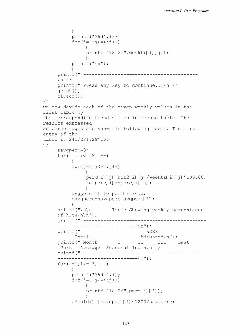
Annexure-I: C++ Programs
143
{ printf("%5d",i); for(j=1;j<=4;j++) { printf("%8.2f",weektr[i][j]); } printf("\n"); } printf(" ---------------------------------------- \n"); printf(" Press any key to continue...\n"); getch(); clrscr(); /* we now devide each of the given weekly values in the first table by the corresponding trend values in second table. The results expressed as percentages are shown in following table. The first entry of the table is 241/281.28*100 */ savgperc=0; for(i=1;i<=12;i++) { for(j=1;j<=4;j++) { perc[i][j]=hit2[i][j]/weektr[i][j]*100.00; totperc[i]+=perc[i][j]; } avgperc[i]=totperc[i]/4.0; savgperc=savgperc+avgperc[i]; } printf("\n\n Table Showing weekly percentages of hits\n\n"); printf(" ------------------------------------------- ----------------------------\n"); printf(" WEEK Total Adjusted\n"); printf(" Month I II III Last
Perc Average Seasonal Index\n"); printf(" -------------------------------------------
----------------------------\n"); for(i=1;i<=12;i++) { printf("%5d ",i); for(j=1;j<=4;j++) { printf("%8.2f",perc[i][j]); } adjsidx[i]=avgperc[i]*1200/savgperc;
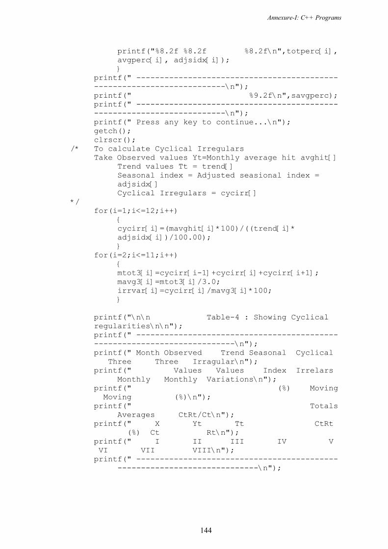
Annexure-I: C++ Programs
144
printf("%8.2f %8.2f %8.2f\n",totperc[i], avgperc[i], adjsidx[i]); } printf(" ------------------------------------------- ----------------------------\n"); printf(" %9.2f\n",savgperc); printf(" ------------------------------------------- ----------------------------\n"); printf(" Press any key to continue...\n"); getch(); clrscr(); /* To calculate Cyclical Irregulars Take Observed values Yt=Monthly average hit avghit[] Trend values Tt = trend[] Seasonal index = Adjusted seasional index = adjsidx[] Cyclical Irregulars = cycirr[] */ for(i=1;i<=12;i++) { cycirr[i]=(mavghit[i]*100)/((trend[i]*
adjsidx[i])/100.00); } for(i=2;i<=11;i++) { mtot3[i]=cycirr[i-1]+cycirr[i]+cycirr[i+1]; mavg3[i]=mtot3[i]/3.0; irrvar[i]=cycirr[i]/mavg3[i]*100; } printf("\n\n Table-4 : Showing Cyclical regularities\n\n"); printf(" ------------------------------------------- ------------------------------\n"); printf(" Month Observed Trend Seasonal Cyclical
Three Three Irragular\n"); printf(" Values Values Index Irrelars Monthly Monthly Variations\n"); printf(" (%) Moving
Moving (%)\n"); printf(" Totals Averages CtRt/Ct\n"); printf(" X Yt Tt CtRt (%) Ct Rt\n"); printf(" I II III IV V VI VII VIII\n"); printf(" ------------------------------------------- ------------------------------\n");

Annexure-I: C++ Programs
145
for(i=1;i<=12;i++) { printf(" %5d%9.2f%9.2f%9.2f %9.2f%9.2f %9.2f %10.4f\n",i, mavghit[i], trend[i], adjsidx[i],cycirr[i],mtot3[i], mavg3[i], irrvar[i]); fprintf(fp2,"%d,%f,%f,%f,%f,%f,%f\n",i,
mavghit[i],trend[i],adjsidx[i],cycirr[i], mavg3[i],irrvar[i]);
} printf(" ------------------------------------------- ------------------------------\n"); printf(" Press any key to continue...\n"); getch(); clrscr(); } 6. irramt.cpp /* Monthly, Weekly number of hits for time series 1st week- Date 1 to 7 2nd week= Date 8 to 14 3rd week- Date 16 to 21 Last week- Date 22 to end of the month Program to calculate monthly trend using least square method*/ #include <stdio.h> # include <conio.h> main() { FILE *fp1,*fp2,*fp3; struct atm { int sr; int yy; int mm; int dd; long int dt; double tm; double amt; }; struct atm day; int tmpmm; int i,j,k; double amt2[13][5]={{0},{0}},mtotamt[13]={0}; double mavgamt[13]={0},xdev[13],xdev2[13];
double xdevy[13],trend[13], irrvar[13]={0}; double weektr[13][5],perc[13][5],totperc[13]={0};
double avgperc[13],savgperc, adjsidx[13];
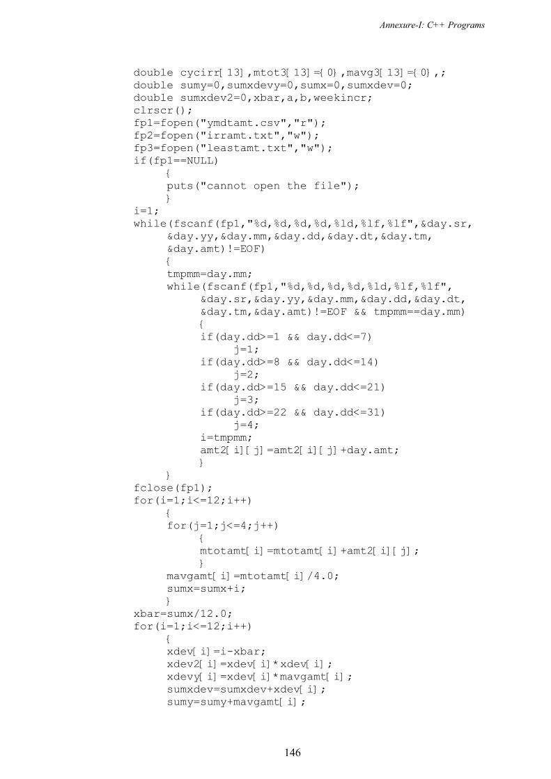
Annexure-I: C++ Programs
146
double cycirr[13],mtot3[13]={0},mavg3[13]={0},; double sumy=0,sumxdevy=0,sumx=0,sumxdev=0;
double sumxdev2=0,xbar,a,b,weekincr; clrscr(); fp1=fopen("ymdtamt.csv","r"); fp2=fopen("irramt.txt","w"); fp3=fopen("leastamt.txt","w"); if(fp1==NULL) { puts("cannot open the file"); } i=1; while(fscanf(fp1,"%d,%d,%d,%d,%ld,%lf,%lf",&day.sr,
&day.yy,&day.mm,&day.dd,&day.dt,&day.tm, &day.amt)!=EOF)
{ tmpmm=day.mm; while(fscanf(fp1,"%d,%d,%d,%d,%ld,%lf,%lf",
&day.sr,&day.yy,&day.mm,&day.dd,&day.dt, &day.tm,&day.amt)!=EOF && tmpmm==day.mm)
{ if(day.dd>=1 && day.dd<=7) j=1; if(day.dd>=8 && day.dd<=14) j=2; if(day.dd>=15 && day.dd<=21) j=3; if(day.dd>=22 && day.dd<=31) j=4; i=tmpmm; amt2[i][j]=amt2[i][j]+day.amt; } } fclose(fp1); for(i=1;i<=12;i++) { for(j=1;j<=4;j++) { mtotamt[i]=mtotamt[i]+amt2[i][j]; } mavgamt[i]=mtotamt[i]/4.0; sumx=sumx+i; } xbar=sumx/12.0; for(i=1;i<=12;i++) { xdev[i]=i-xbar; xdev2[i]=xdev[i]*xdev[i]; xdevy[i]=xdev[i]*mavgamt[i]; sumxdev=sumxdev+xdev[i]; sumy=sumy+mavgamt[i];

Annexure-I: C++ Programs
147
sumxdev2=sumxdev2+xdev2[i]; sumxdevy=sumxdevy+xdevy[i]; } a=sumy/12.0; b=sumxdevy/sumxdev2; for(i=1;i<=12;i++) trend[i]=a+b*xdev[i]; printf("\n weekly total amount withdrawn\n\n"); printf(" ------------------------------------------- --------\n"); printf(" Month WEEK \n"); printf(" ------------------------------ \n"); printf(" X Xdev I II III Last
Total\n"); printf(" ------------------------------------------- --------\n"); for(i=1;i<=12;i++) { printf(" %5d%6.2lf",i,xdev[i]); for(j=1;j<=4;j++) { printf("%8.0lf",amt2[i][j]); } printf("%8.0lf\n",mtotamt[i]); } printf(" ------------------------------------------- --------\n"); printf(" %6.2lf\n",sumxdev); printf(" ------------------------------------------- --------\n"); printf(" Press any key to continue....\n"); getch(); clrscr(); printf("\n\n Least square method for weekly total amount withdrawn\n\n"); printf(" ------------------------------------------- --------------------------\n"); printf(" Weekly\n"); printf(" Month Weekly Average TrendY\n"); printf(" X Xdev Total Y Xdev^2 XdevY a+b*xdev\n"); printf(" ------------------------------------------- --------------------------\n"); for(i=1;i<=12;i++) { printf(" %5d%6.2lf",i,xdev[i]); printf(" %12.2lf%12.2lf%8.2lf%13.2lf%12.2lf\n",
mtotamt[i mavgamt[i],xdev2[i],xdevy[i],

Annexure-I: C++ Programs
148
trend[i]); fprintf(fp3,"%d,%12.2lf\n",i,trend[i]); } printf(" ------------------------------------------- --------------------------\n"); printf(" %6.2lf %12.2lf%8.2lf%13.2lf\n",
sumxdev,sumy,sumxdev2,sumxdevy); printf(" ------------------------------------------- --------------------------\n"); printf("\n a=%-12.2lf b=%-12.2lf\n",a,b); printf("\n Press any key to continue....\n"); fclose(fp3); getch(); clrscr(); weekincr=b/4.0; k=0; for(i=7;i<=12;i++) for(j=1;j<=4;j++) { weektr[i][j]=amt2[7][1]+k*weekincr; k++; } k=1; for(i=6;i>=1;i--) for(j=4;j>=1;j--) { weektr[i][j]=amt2[7][1]-k*weekincr; k++; } printf(" Table showing weekly trend of amount withdrawn\n\n"); printf("-------------------------------------------- ---------\n"); printf(" WEEK\n"); printf("Month I II III
Last \n"); printf("-------------------------------------------- ---------\n"); for(i=1;i<=12;i++) { printf("%5d",i); for(j=1;j<=4;j++) { printf("%12.2lf",weektr[i][j]); } printf("\n"); } printf("-------------------------------------------- ---------\n"); printf("Press any key to continue...\n"); getch();
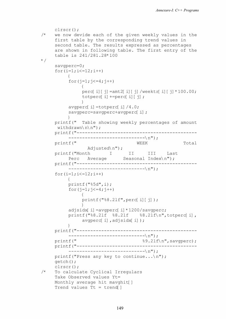
Annexure-I: C++ Programs
149
clrscr(); /* we now devide each of the given weekly values in the first table by the corresponding trend values in
second table. The results expressed as percentages are shown in following table. The first entry of the
table is 241/281.28*100 */ savgperc=0; for(i=1;i<=12;i++) { for(j=1;j<=4;j++) { perc[i][j]=amt2[i][j]/weektr[i][j]*100.00; totperc[i]+=perc[i][j]; } avgperc[i]=totperc[i]/4.0; savgperc=savgperc+avgperc[i]; } printf(" Table showing weekly percentages of amount
withdrawn\n\n"); printf("-------------------------------------------- ----------------------------\n"); printf(" WEEK Total Adjusted\n"); printf("Month I II III Last Perc Average Seasonal Index\n"); printf("-------------------------------------------- ----------------------------\n"); for(i=1;i<=12;i++) { printf("%5d",i); for(j=1;j<=4;j++) { printf("%8.2lf",perc[i][j]); } adjsidx[i]=avgperc[i]*1200/savgperc; printf("%8.2lf %8.2lf %8.2lf\n",totperc[i], avgperc[i],adjsidx[i]); } printf("-------------------------------------------- ----------------------------\n"); printf(" %9.2lf\n",savgperc); printf("-------------------------------------------- ----------------------------\n"); printf("Press any key to continue...\n"); getch(); clrscr(); /* To calculate Cyclical Irregulars Take Observed values Yt=
Monthly average hit mavghit[] Trend values Tt = trend[]
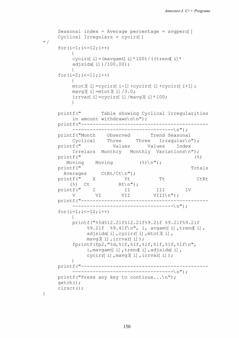
Annexure-I: C++ Programs
150
Seasonal index = Average percentage = avgperc[] Cyclical Irregulars = cycirr[] */ for(i=1;i<=12;i++) { cycirr[i]=(mavgamt[i]*100)/((trend[i]*
adjsidx[i])/100.00); } for(i=2;i<=11;i++) { mtot3[i]=cycirr[i-1]+cycirr[i]+cycirr[i+1]; mavg3[i]=mtot3[i]/3.0; irrvar[i]=cycirr[i]/mavg3[i]*100; } printf(" Table showing Cyclical Irregularities in amount withdrawn\n\n"); printf("-------------------------------------------- -----------------------------------\n"); printf("Month Observed Trend Seasonal Cyclical Three Three Irragular\n"); printf(" Values Values Index Irrelars Monthly Monthly Variations\n"); printf(" (%)
Moving Moving (%)\n"); printf(" Totals
Averages CtRt/Ct\n"); printf(" X Yt Tt CtRt
(%) Ct Rt\n"); printf(" I II III IV V VI VII VIII\n"); printf("-------------------------------------------- -----------------------------------\n"); for(i=1;i<=12;i++) { printf("%5d%12.2lf%12.2lf%9.2lf %9.2lf%9.2lf %9.2lf %9.4lf\n", i, avgamt[i],trend[i],
adjsidx[i],cycirr[i],mtot3[i], mavg3[i],irrvar[i]); fprintf(fp2,"%d,%lf,%lf,%lf,%lf,%lf,%lf\n",
i,mavgamt[i],trend[i],adjsidx[i], cycirr[i],mavg3[i],irrvar[i]);
} printf("-------------------------------------------- -----------------------------------\n"); printf("Press any key to continue...\n"); getch(); clrscr(); }
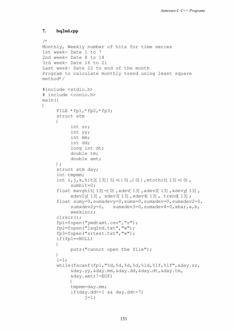
Annexure-I: C++ Programs
151
7. lsq2nd.cpp /* Monthly, Weekly number of hits for time series 1st week- Date 1 to 7 2nd week= Date 8 to 14 3rd week- Date 16 to 21 Last week- Date 22 to end of the month Program to calculate monthly trend using least square method*/ #include <stdio.h> # include <conio.h> main() { FILE *fp1,*fp2,*fp3; struct atm { int sr; int yy; int mm; int dd; long int dt; double tm; double amt; }; struct atm day; int tmpmm; int i,j,k,hit2[13][5]={{0},{0}},mtothit[13]={0},
sumhit=0; float mavghit[13]={0},xdev[13],xdev2[13],xdevy[13],
xdev2y[13], xdev3[13],xdev4[13], trend[13]; float sumy=0,sumxdevy=0,sumx=0,sumxdev=0,sumxdev2=0,
sumxdev2y=0, sumxdev3=0,sumxdev4=0,xbar,a,b, weekincr;
clrscr(); fp1=fopen("ymdtamt.csv","r"); fp2=fopen("lsq2nd.txt","w"); fp3=fopen("srtest.txt","w"); if(fp1==NULL) { puts("cannot open the file"); } i=1; while(fscanf(fp1,"%d,%d,%d,%d,%ld,%lf,%lf",&day.sr,
&day.yy,&day.mm,&day.dd,&day.dt,&day.tm, &day.amt)!=EOF)
{ tmpmm=day.mm; if(day.dd>=1 && day.dd<=7) j=1;

Annexure-I: C++ Programs
152
if(day.dd>=8 && day.dd<=14) j=2; if(day.dd>=15 && day.dd<=21) j=3; if(day.dd>=22 && day.dd<=31) j=4; i=tmpmm; hit2[i][j]++; fprintf(fp3,"%d\n",day.sr); while(fscanf(fp1,"%d,%d,%d,%d,%ld,%lf,%lf",
&day.sr,&day.yy,&day.mm,&day.dd,&day.dt, &day.tm,&day.amt)!=EOF && mpmm==day.mm)
{ if(day.dd>=1 && day.dd<=7) j=1; if(day.dd>=8 && day.dd<=14) j=2; if(day.dd>=15 && day.dd<=21) j=3; if(day.dd>=22 && day.dd<=31) j=4; i=tmpmm; hit2[i][j]++; fprintf(fp3,"%d\n",day.sr); } if(day.dd>=1 && day.dd<=7) j=1; if(day.dd>=8 && day.dd<=14) j=2; if(day.dd>=15 && day.dd<=21) j=3; if(day.dd>=22 && day.dd<=31) j=4; i=day.mm; hit2[i][j]++; fprintf(fp3,"%d\n",day.sr); } hit2[i][j]--; fclose(fp1); fclose(fp3); for(i=1;i<=12;i++) { for(j=1;j<=4;j++) { mtothit[i]=mtothit[i]+hit2[i][j]; } mavghit[i]=mtothit[i]/4.0; sumhit=sumhit+mtothit[i]; sumx=sumx+i; } xbar=sumx/12.0;

Annexure-I: C++ Programs
153
for(i=1;i<=12;i++) { xdev[i]=i-xbar; xdev2[i]=xdev[i]*xdev[i]; xdev3[i]=xdev2[i]*xdev[i]; xdev4[i]=xdev3[i]*xdev[i]; xdevy[i]=xdev[i]*mavghit[i]; xdev2y[i]=xdevy[i]*xdev[i]; sumxdev=sumxdev+xdev[i]; sumy=sumy+mavghit[i]; sumxdev2=sumxdev2+xdev2[i]; sumxdevy=sumxdevy+xdevy[i]; sumxdev2y=sumxdev2y+xdev2y[i]; sumxdev3=sumxdev3=xdev3[i]; sumxdev4=sumxdev4+xdev4[i]; } printf("\n\n Table Showing feeting of second degree curve\n\n"); printf(" ------------------------------------------- -----------------------------------\n"); printf(" WEEK \n"); printf(" Month ----------------- Avg \n"); printf(" X Xdev I II III Last Tot Y Xdev^2 Xdev^3 Xdev^4 XdevY Xdev^2y\n"); printf(" ------------------------------------------- -----------------------------------\n"); for(i=1;i<=12;i++) { printf("%4d%6.2f",i,xdev[i]); for(j=1;j<=4;j++) { printf("%4d",hit2[i][j]); } printf(" %4d %7.2f%7.2f%8.2f%8.2f%8.2f
%9.2f\n",mtothit[i], mavghit[i], xdev2[i], xdev3[i],xdev4[i],xdevy[i],xdev2y[i]);
fprintf(fp2,"%d%8.2f%8.2f\n",i,xdev[i], xdev2[i]);
} printf(" ------------------------------------------- -----------------------------------\n"); printf(" %6.2f %5d %7.2f %6.2f
%7.2f%8.2f%8.2f %9.2f \n", sumxdev,sumhit,sumy, sumxdev2,sumxdev3,sumxdev4, sumxdevy, sumxdev2y);
printf(" ------------------------------------------- -----------------------------------\n"); printf(" Press any key to continue....\n"); fclose(fp1); getch(); clrscr(); }
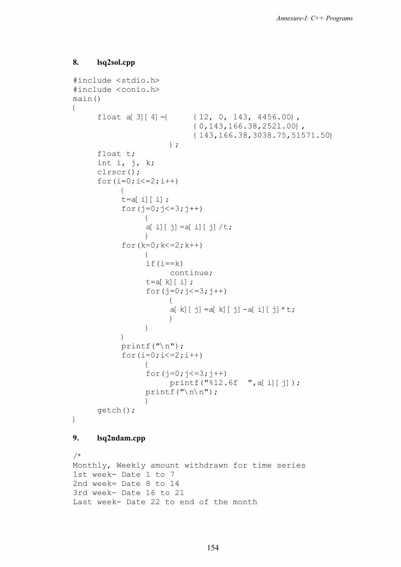
Annexure-I: C++ Programs
154
8. lsq2sol.cpp #include <stdio.h> #include <conio.h> main() { float a[3][4]={ {12, 0, 143, 4456.00}, {0,143,166.38,2521.00}, {143,166.38,3038.75,51571.50} }; float t; int i, j, k; clrscr(); for(i=0;i<=2;i++) { t=a[i][i]; for(j=0;j<=3;j++) { a[i][j]=a[i][j]/t; } for(k=0;k<=2;k++) { if(i==k) continue; t=a[k][i]; for(j=0;j<=3;j++) { a[k][j]=a[k][j]-a[i][j]*t; } } } printf("\n"); for(i=0;i<=2;i++) { for(j=0;j<=3;j++) printf("%12.6f ",a[i][j]); printf("\n\n"); } getch(); } 9. lsq2ndam.cpp /* Monthly, Weekly amount withdrawn for time series 1st week- Date 1 to 7 2nd week= Date 8 to 14 3rd week- Date 16 to 21 Last week- Date 22 to end of the month

Annexure-I: C++ Programs
155
Program to calculate monthly trend using least square method*/ #include <stdio.h> # include <conio.h> main() { FILE *fp1,*fp2,*fp3; struct atm { int sr; int yy; int mm; int dd; long int dt; double tm; double amt; }; struct atm day; int tmpmm; int i,j,k; long int amt2[13][5]={{0},{0}},mtotamt[13]={0},
sumamt=0; double mavgamt[13]={0},xdev[13],xdev2[13],xdevy[13],
xdev2y[13], xdev3[13],xdev4[13],trend[13]; double sumy=0,sumxdevy=0,sumx=0,sumxdev=0,
sumxdev2=0,sumxdev2y=0,sumxdev3=0,sumxdev4=0, xbar,a,b,weekincr;
clrscr(); fp1=fopen("ymdtamt.csv","r"); fp2=fopen("lsq2ndam.txt","w"); if(fp1==NULL) { puts("cannot open the file"); } i=1; while(fscanf(fp1,"%d,%d,%d,%d,%ld,%lf,%lf",&day.sr,
&day.yy,&day.mm,&day.dd,&day.dt,&day.tm, &day.amt)!=EOF)
{ tmpmm=day.mm; while(fscanf(fp1,"%d,%d,%d,%d,%ld,%lf,%lf",
&day.sr,&day.yy,&day.mm,&day.dd,&day.dt, &day.tm,&day.amt)!=EOF&&tmpmm==day.mm)
{ if(day.dd>=1 && day.dd<=7) j=1; if(day.dd>=8 && day.dd<=14) j=2; if(day.dd>=15 && day.dd<=21) j=3;

Annexure-I: C++ Programs
156
if(day.dd>=22 && day.dd<=31) j=4; i=tmpmm; amt2[i][j]=amt2[i][j]+day.amt; } } fclose(fp1); for(i=1;i<=12;i++) { for(j=1;j<=4;j++) { mtotamt[i]=mtotamt[i]+amt2[i][j]; } mavgamt[i]=mtotamt[i]/4.0; sumamt=sumamt+mtotamt[i]; sumx=sumx+i; } xbar=sumx/12.0; for(i=1;i<=12;i++) { xdev[i]=i-xbar; xdev2[i]=xdev[i]*xdev[i]; xdev3[i]=xdev2[i]*xdev[i]; xdev4[i]=xdev3[i]*xdev[i]; xdevy[i]=xdev[i]*mavgamt[i]; xdev2y[i]=xdevy[i]*xdev[i]; sumxdev=sumxdev+xdev[i]; sumy=sumy+mavgamt[i]; sumxdev2=sumxdev2+xdev2[i]; sumxdevy=sumxdevy+xdevy[i]; sumxdev2y=sumxdev2y+xdev2y[i]; sumxdev3=sumxdev3=xdev3[i]; sumxdev4=sumxdev4+xdev4[i]; } printf("\n\n Table showing feeting of second degree curve\n\n"); printf(" ------------------------------------------- ---------------------------\n"); printf(" WEEK \n"); printf(" Month ----------------------------- ----- Avg \n"); printf(" X Xdev I II III
Last Tot Y \n"); printf(" ------------------------------------------- ---------------------------\n"); for(i=1;i<=12;i++) { printf(" %4d %6.2lf",i,xdev[i]); for(j=1;j<=4;j++) {

Annexure-I: C++ Programs
157
printf("%9ld",amt2[i][j]); } printf(" %9ld%12.2lf\n",mtotamt[i],mavgamt[i]); } printf(" ------------------------------------------- ---------------------------\n"); printf(" %6.2lf %9ld\n",
sumxdev, sumamt); printf(" ------------------------------------------- ---------------------------\n"); printf("\n\n Table showing feeting of second degree curve\n\n"); printf(" ------------------------------------------- --------------------------------\n"); printf(" Month Avg\n"); printf(" X Xdev Y Xdev^2 Xdev^3
Xdev^4 XdevY Xdev^2y\n"); printf(" ------------------------------------------- --------------------------------\n"); for(i=1;i<=12;i++) { printf(" %4d%6.2lf",i,xdev[i]); printf("%12.2lf%8.2lf%8.2lf%8.2lf%14.2lf
%14.2lf\n",mavgamt[i],xdev2[i],xdev3[i], xdev4[i],xdevy[i],xdev2y[i]);
fprintf(fp2,"%d%8.2lf%8.2lf\n",i,xdev[i], xdev2[i]);
} printf(" ------------------------------------------- --------------------------------\n"); printf(" %6.2lf%12.2lf%8.2lf%8.2lf%8.2lf%14.2lf
%14.2lf\n", sumxdev,sumy, sumxdev2,sumxdev3, sumxdev4,sumxdevy,sumxdev2y);
printf(" ------------------------------------------- --------------------------------\n"); printf(" Press any key to continue....\n"); fclose(fp1); getch(); clrscr(); } 10. lsq2sola.cpp #include <stdio.h> #include <conio.h> main() { float a[3][4]=
{ {12, 0, 143, 15922262.5}, {0,143,166.38,9698503.75}, {143,166.38,3038.75,187656900.62}
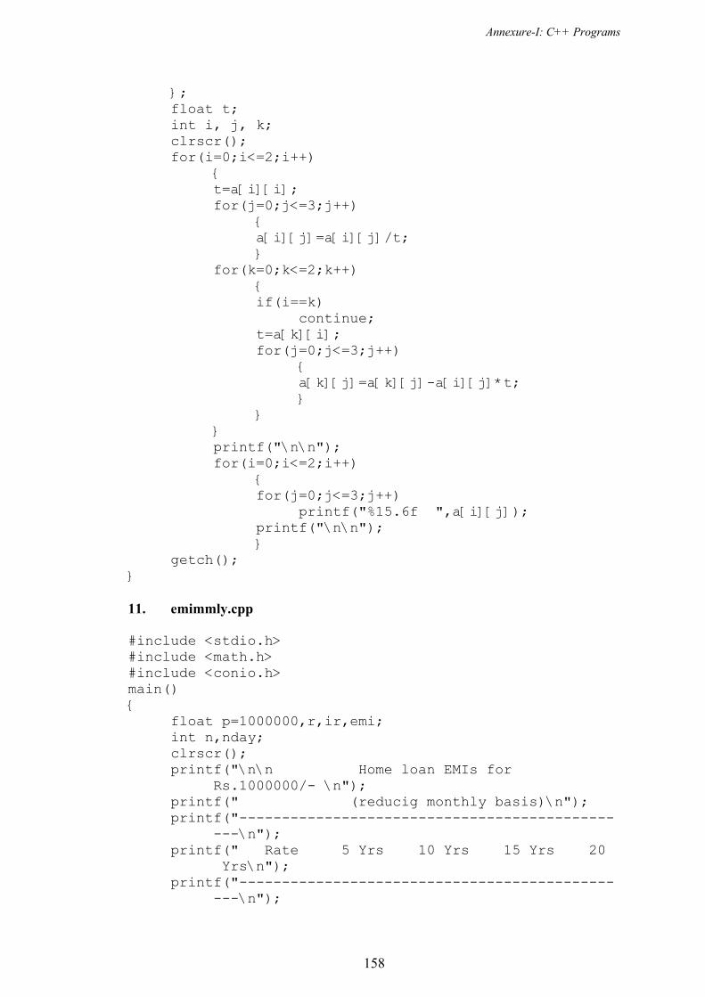
Annexure-I: C++ Programs
158
}; float t; int i, j, k; clrscr(); for(i=0;i<=2;i++) { t=a[i][i]; for(j=0;j<=3;j++) { a[i][j]=a[i][j]/t; } for(k=0;k<=2;k++) { if(i==k) continue; t=a[k][i]; for(j=0;j<=3;j++) { a[k][j]=a[k][j]-a[i][j]*t; } } } printf("\n\n"); for(i=0;i<=2;i++) { for(j=0;j<=3;j++) printf("%15.6f ",a[i][j]); printf("\n\n"); } getch(); } 11. emimmly.cpp #include <stdio.h> #include <math.h> #include <conio.h> main() { float p=1000000,r,ir,emi; int n,nday; clrscr(); printf("\n\n Home loan EMIs for Rs.1000000/- \n"); printf(" (reducig monthly basis)\n"); printf("-------------------------------------------- ---\n"); printf(" Rate 5 Yrs 10 Yrs 15 Yrs 20
Yrs\n"); printf("-------------------------------------------- ---\n");
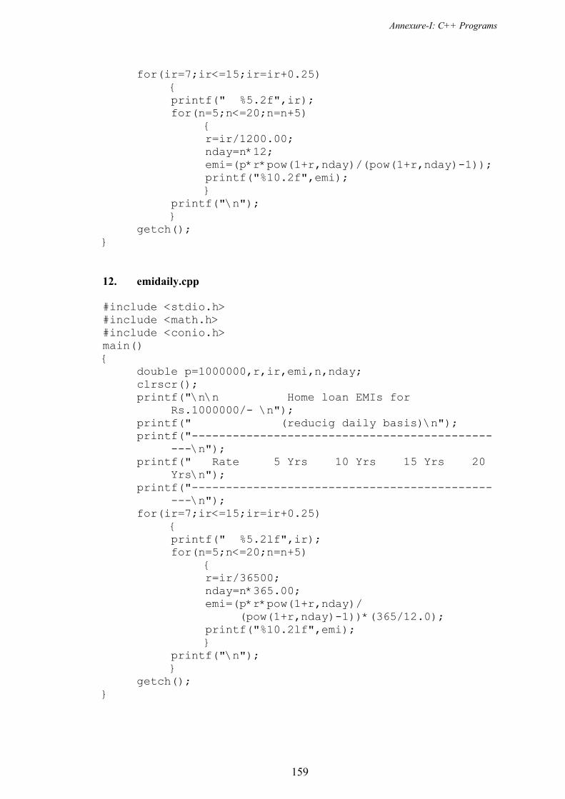
Annexure-I: C++ Programs
159
for(ir=7;ir<=15;ir=ir+0.25) { printf(" %5.2f",ir); for(n=5;n<=20;n=n+5) { r=ir/1200.00; nday=n*12; emi=(p*r*pow(1+r,nday)/(pow(1+r,nday)-1)); printf("%10.2f",emi); } printf("\n"); } getch(); } 12. emidaily.cpp #include <stdio.h> #include <math.h> #include <conio.h> main() { double p=1000000,r,ir,emi,n,nday; clrscr(); printf("\n\n Home loan EMIs for Rs.1000000/- \n"); printf(" (reducig daily basis)\n"); printf("-------------------------------------------- ---\n"); printf(" Rate 5 Yrs 10 Yrs 15 Yrs 20 Yrs\n"); printf("-------------------------------------------- ---\n"); for(ir=7;ir<=15;ir=ir+0.25) { printf(" %5.2lf",ir); for(n=5;n<=20;n=n+5) { r=ir/36500; nday=n*365.00; emi=(p*r*pow(1+r,nday)/
(pow(1+r,nday)-1))*(365/12.0); printf("%10.2lf",emi); } printf("\n"); } getch(); }

Annexure-I: C++ Programs
160
13. emidiff.cpp #include <stdio.h> #include <math.h> #include <conio.h> main() { float p=1000000,r,ir,emimm,emidd,diff; int n,nday; FILE *fp; clrscr(); fp=fopen("emidiff.txt","w"); printf("\n\n Home loan of
Rs.1000000/- \n"); printf(" Statement showing EMIs on reducig monthly basis, daily basis and difference\n"); printf(" ------------------------------------------- -----------------------------------\n"); printf(" 5 Yrs 10 Yrs
15 Yrs 20 Yrs\n"); printf(" ------------------------------------ -----------------------------------\n"); printf(" Rate mnthly daily diff mnthly daily diff mnthly daily diff mnthly daily diff\n"); printf(" ------------------------------------------- -----------------------------------\n"); for(ir=7;ir<=15;ir=ir+0.25) { printf(" %5.2f",ir); fprintf(fp,"%5.2f,",ir); for(n=5;n<=20;n=n+5) { r=ir/1200; nday=n*12; emimm=(p*r*pow(1+r,nday)/
(pow(1+r,nday)-1)); r=ir/36500; nday=n*365; emidd=(p*r*pow(1+r,nday)/
(pow(1+r,nday)-1))*(365/12.0); diff=(emimm-emidd)*n*12; printf("%7.f%6.f%5.f",emimm,emidd,diff); fprintf(fp,"%7.f,%7.f,%7.f,",
emimm,emidd,diff); } printf("\n"); fprintf(fp,"\n"); } fclose(fp); getch(); }

Annexure-I: C++ Programs
161
14. emicheck.cpp # include <math.h> # include <stdio.h> # include <conio.h> main() { int i; double p,r,n,n1,e,eamt,openbal,adjp,adjint,closbal; clrscr(); p=1000000; r=11; n=5; n1=n*12; e=21742.00; eamt=e*pow((1.00+r/36500.00),(365.00/24.00)); printf("\n\n Loan amount:%10.2lf\n",p); printf(" Rate of Interest:%10.2lf\n",r); printf(" EMI on Monthly basis:%10.2lf\n",e); printf(" EMI+15 days interest:%10.2lf\n",eamt); openbal=p; printf(" ------------------------------------------- -----------\n"); printf(" Month Opening Adjusted Adjusted Closing\n"); printf(" Balance Principal Interest Balance\n"); printf(" ------------------------------------------- -----------\n"); for(i=1;i<=n1;i++) { adjint=openbal*pow((1+r/36500.00),(365.00/12))- openbal; adjp=eamt-adjint; closbal=openbal-adjp; printf(" %5d %12.2lf%12.2lf%12.2lf%12.2lf\n",
i,openbal,adjp,adjint,closbal); openbal=closbal; if(i%30==0) { getch(); clrscr(); printf(" --------------------------------- ---------------------\n"); printf(" Month Opening Adjusted
Adjusted Closing\n"); printf(" Balance Principal
Interest Balance\n"); printf(" ---------------------------------
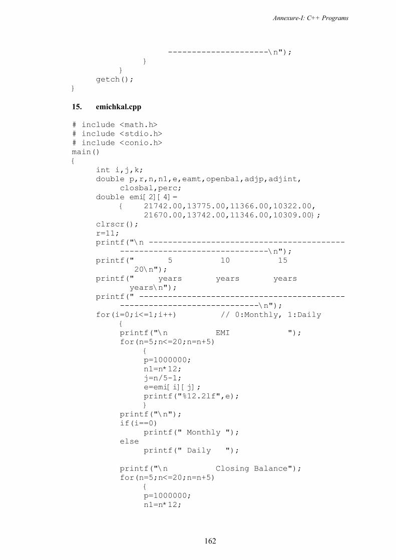
Annexure-I: C++ Programs
162
---------------------\n"); } } getch(); } 15. emichkal.cpp # include <math.h> # include <stdio.h> # include <conio.h> main() { int i,j,k; double p,r,n,n1,e,eamt,openbal,adjp,adjint,
closbal,perc; double emi[2][4]=
{ 21742.00,13775.00,11366.00,10322.00, 21670.00,13742.00,11346.00,10309.00}; clrscr(); r=11; printf("\n ----------------------------------------- -------------------------------\n"); printf(" 5 10 15
20\n"); printf(" years years years
years\n"); printf(" ------------------------------------------- -----------------------------\n"); for(i=0;i<=1;i++) // 0:Monthly, 1:Daily { printf("\n EMI "); for(n=5;n<=20;n=n+5) { p=1000000; n1=n*12; j=n/5-1; e=emi[i][j]; printf("%12.2lf",e); } printf("\n"); if(i==0) printf(" Monthly "); else printf(" Daily "); printf("\n Closing Balance"); for(n=5;n<=20;n=n+5) { p=1000000; n1=n*12;

Annexure-I: C++ Programs
163
j=n/5-1; e=emi[i][j]; eamt=e*pow((1.00+r/36500.00),
(365.00/24.00)); openbal=p; for(k=1;k<=n1;k++) { adjint=openbal*pow((1+r/36500.00),
(365.00/12))- openbal; adjp=eamt-adjint; closbal=openbal-adjp; openbal=closbal; } printf("%12.2lf",closbal); } printf("\n\n"); } printf(" ------------------------------------------- -----------------------------\n"); getch(); } 16. fdqtrly.cpp #include <stdio.h> #include <math.h> #include <conio.h> main() { float p=100000,r,ir,amtq,nt; int n; clrscr(); printf("\n\n Fixed Deposite of Rs.100000/- \n"); printf(" Statement showing Amount returned on Quarterly compounded basis\n"); printf(" ------------------------------------------- --------------------------------\n"); printf(" PERIOD IN MONTHS\n"); printf(" -------------------------------------- --------------------------------\n"); printf(" Rate 12 15 18
21 24 27 30\n"); printf(" ------------------------------------------- --------------------------------\n"); for(ir=6;ir<=10;ir=ir+0.25) { printf(" %5.2f",ir); for(n=12;n<=30;n=n+3) { r=ir/400;

Annexure-I: C++ Programs
164
nt=4.0*(n/12.0); amtq=p*pow(1+r,nt); printf("%10.2f",amtq); } printf("\n"); } printf(" ------------------------------------------- --------------------------------\n"); printf(" Rate 33 36 39
42 45 48 51\n"); printf(" ------------------------------------------- --------------------------------\n"); for(ir=6;ir<=10;ir=ir+0.25) { printf(" %5.2f",ir); for(n=33;n<=51;n=n+3) { r=ir/400; nt=4.0*(n/12.0); amtq=p*pow(1+r,nt); printf("%10.2f",amtq); } printf("\n"); } getch(); } 17. fddaily.cpp #include <stdio.h> #include <math.h> #include <conio.h> main() { float p=100000,r,ir,amtd,nt; int n; clrscr(); printf("\n\n Fixed Deposite of Rs.100000/- \n"); printf(" Statement showing Amount returned on Daily compounded basis\n"); printf(" ------------------------------------------- --------------------------------\n"); printf(" PERIOD IN MONTHS\n"); printf(" -------------------------------------- --------------------------------\n"); printf(" Rate 12 15 18 21
24 27 30\n"); printf(" ------------------------------------------- --------------------------------\n"); for(ir=6;ir<=10;ir=ir+0.25) {

Annexure-I: C++ Programs
165
printf(" %5.2f",ir); for(n=12;n<=30;n=n+3) { r=ir/36500; nt=365.0*(n/12.0); amtd=p*pow(1+r,nt); printf("%10.2f",amtd); } printf("\n"); } printf(" ------------------------------------------- --------------------------------\n"); printf(" Rate 33 36 39 42
45 48 51\n"); printf(" ------------------------------------------- --------------------------------\n"); for(ir=6;ir<=10;ir=ir+0.25) { printf(" %5.2f",ir); for(n=33;n<=51;n=n+3) { r=ir/36500; nt=365.0*(n/12.0); amtd=p*pow(1+r,nt); printf("%10.2f",amtd); } printf("\n"); } getch(); } 18. fddiff.cpp #include <stdio.h> #include <math.h> #include <conio.h> main() { float p=100000,r,ir,amtd,amtq,diff,nt; int n; clrscr(); printf("\n\n Fixed Deposite of Rs.100000/- \n"); printf(" Statement showing difference of maturity amount returned on\n"); printf(" Daily and Quarterly compounded basis\n"); printf(" ------------------------------------------- --------------------------------\n"); printf(" PERIOD IN MONTHS\n"); printf(" -------------------------------------- --------------------------------\n");

Annexure-I: C++ Programs
166
printf(" Rate 12 15 18 21 24 27 30\n");
printf(" ------------------------------------------- --------------------------------\n"); for(ir=6;ir<=10;ir=ir+0.25) { printf(" %5.2f",ir); for(n=12;n<=30;n=n+3) { r=ir/36500; nt=365.0*(n/12.0); amtd=p*pow(1+r,nt); r=ir/400; nt=4.0*(n/12.0); amtq=p*pow(1+r,nt); diff=amtd-amtq; printf("%10.2f",diff); } printf("\n"); } printf(" ------------------------------------------- --------------------------------\n"); printf(" Rate 33 36 39 42
45 48 51\n"); printf(" ------------------------------------------- -------------------------------\n"); for(ir=6;ir<=10;ir=ir+0.25) { printf(" %5.2f",ir); for(n=33;n<=51;n=n+3) { r=ir/36500; nt=365.0*(n/12.0); amtd=p*pow(1+r,nt); r=ir/400; nt=4.0*(n/12.0); amtq=p*pow(1+r,nt); diff=amtd-amtq; printf("%10.2f",diff); } printf("\n"); } getch(); } 19. recurqfl.cpp #include <stdio.h> #include <conio.h> #include <math.h> void main()
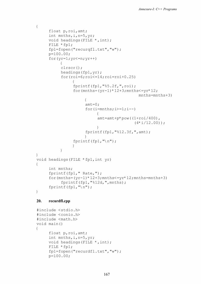
Annexure-I: C++ Programs
167
{ float p,roi,amt; int mnths,i,n=5,yr; void headings(FILE *,int); FILE *fp1; fp1=fopen("recurqfl.txt","w"); p=100.00; for(yr=1;yr<=n;yr++) { clrscr(); headings(fp1,yr); for(roi=6;roi<=14;roi=roi+0.25) { fprintf(fp1,"%5.2f,",roi); for(mnths=(yr-1)*12+3;mnths<=yr*12;
mnths=mnths+3) { amt=0; for(i=mnths;i>=1;i--) { amt=amt+p*pow((1+roi/400),
(4*i/12.00)); } fprintf(fp1,"%12.3f,",amt); } fprintf(fp1,"\n"); } } } void headings(FILE *fp1,int yr) { int mnths; fprintf(fp1," Rate,"); for(mnths=(yr-1)*12+3;mnths<=yr*12;mnths=mnths+3) fprintf(fp1,"%12d,",mnths); fprintf(fp1,"\n"); } 20. recurdfl.cpp #include <stdio.h> #include <conio.h> #include <math.h> void main() { float p,roi,amt; int mnths,i,n=5,yr; void headings(FILE *,int); FILE *fp1; fp1=fopen("recurdfl.txt","w"); p=100.00;

Annexure-I: C++ Programs
168
for(yr=1;yr<=n;yr++) { clrscr(); headings(fp1,yr); for(roi=6;roi<=14;roi=roi+0.25) { fprintf(fp1,"%5.2f,",roi); for(mnths=(yr-1)*12+3;mnths<=yr*12;
mnths=mnths+3) { amt=0; for(i=mnths;i>=1;i--) { amt=amt+p*pow((1+roi/36500),
(365*i/12.00)); } fprintf(fp1,"%12.3f,",amt); } fprintf(fp1,"\n"); } } } void headings(FILE *fp1,int yr) { int mnths; fprintf(fp1," Rate,"); for(mnths=(yr-1)*12+3;mnths<=yr*12;mnths=mnths+3) fprintf(fp1,"%12d,",mnths); fprintf(fp1,"\n"); } 21. recudiff.cpp #include <stdio.h> #include <conio.h> #include <math.h> void main() { float p,roi,amtq,amtd,diff; int mnths,i,n=5,yr; void headings(FILE *,int); FILE *fp1; fp1=fopen("recudiff.txt","w"); p=100.00; for(yr=1;yr<=n;yr++) { clrscr(); headings(fp1,yr); for(roi=6;roi<=14;roi=roi+0.25) { fprintf(fp1,"%5.2f,",roi);

Annexure-I: C++ Programs
169
for(mnths=(yr-1)*12+3;mnths<=yr*12; mnths=mnths+3)
{ amtq=amtd=0; for(i=mnths;i>=1;i--) { amtd=amtd+p*pow((1+roi/36500), (365*i/12.00)); amtq=amtq+p*pow((1+roi/400),
(4*i/12.00)); } diff=amtd-amtq; fprintf(fp1,"%12.3f,",diff); } fprintf(fp1,"\n"); } } } void headings(FILE *fp1,int yr) { int mnths; fprintf(fp1," Rate,"); for(mnths=(yr-1)*12+3;mnths<=yr*12;mnths=mnths+3) fprintf(fp1,"%12d,",mnths); fprintf(fp1,"\n"); } 22. grfile.cpp #include <stdio.h> #include <conio.h> #include <math.h> void main() { FILE *fp1,*fp2; long double ts,tt,sbar,tbar,tmp; long double t0,b0,tb01,tb02; long double as[366],at[366],ab01[366],ab02[366]; long double ay4[366],ty4; /* double tmp;*/ int i,x,ax[366],tx,n=365,tmpi; clrscr(); fp1=fopen("snrdhita.csv","r"); fp2=fopen("graphicl.txt","w"); if(fp1==NULL) { puts("cannot open the file");

Annexure-I: C++ Programs
170
} tmpi=0; tx=0; ts=0.0; tt=0.0; while(fscanf(fp1,"%d,%d",&i,&x)!=EOF) { if(tmpi==i) break; ax[i]=x; as[i]=log(log((n+1)/(float)(n-i+1))); at[i]=log(x); tx=tx+x; ts=ts+as[i]; tt=tt+at[i]; tmpi=i; } sbar=ts/n; tbar=tt/n; fclose(fp1); tb01=tb02=0.0; for(i=1;i<=n;i++) { ab01[i]=(as[i]-sbar)*(at[i]-tbar); tb01=tb01+ab01[i]; ab02[i]=(at[i]-tbar)*(at[i]-tbar); tb02=tb02+ab02[i]; } b0=tb01/tb02; fprintf(fp2,"--------------------------------------- ----------------------------------------------- ---------\n"); fprintf(fp2," i x si ti
(si-sbar)(ti-tbar) (ti-tbar)^2 xi^b0\n"); fprintf(fp2,"--------------------------------------- ----------------------------------------------- ---------\n"); ty4=0.0; for(i=1;i<=n;i++) { tmp=ax[i]; ay4[i]=pow(tmp,b0); ty4=ty4+ay4[i]; fprintf(fp2,"%5d%5d%13.6Lf%13.6Lf
%13.6Lf %13.6Lf %20.6Lf\n", i,ax[i],as[i],at[i],ab01[i],ab02[i],ay4[i]);
} fprintf(fp2,"--------------------------------------- ----------------------------------------------- ---------\n");

Annexure-I: C++ Programs
171
fprintf(fp2,"TOT %5d%13.6Lf%13.6Lf %13.6Lf %13.6Lf %20.6Lf\n",tx,ts,tt,tb01,tb02,ty4);
fprintf(fp2,"--------------------------------------- ----------------------------------------------- ---------\n"); fprintf(fp2," %13.6Lf%13.6Lf\n",sbar,tbar); fprintf(fp2,"--------------------------------------- ----------------------------------------------- ---------\n"); t0=ty4/(long double)n; fprintf(fp2,"\nBeta=%10.7Lf Theta=%17.6Lf\n"
,b0,t0); fclose(fp2); } 23. nrtable1.cpp #include <stdio.h> #include <conio.h> #include <math.h> void main() { FILE *fp1,*fp2; long double ts,tt,sbar,tbar,tmp; long double z1,z2,t0,b0,b1,diff; long double tb01,tb02; long double as[366],at[366],ab01[366],ab02[366]; long double ay1[366],ay2[366],ay3[366],ay4[366],
ty1,ty2,ty3,ty4; /* double tmp;*/ int i,x,ax[366],tx,n=365,tmpi,iteration=1; clrscr(); fp1=fopen("snrdhita.csv","r"); fp2=fopen("nriterja.txt","w"); if(fp1==NULL) { puts("cannot open the file"); } tmpi=0; tx=0; ts=0.0; tt=0.0; while(fscanf(fp1,"%d,%d",&i,&x)!=EOF) { if(tmpi==i) break; ax[i]=x; as[i]=log(log((n+1)/(float)(n-i+1)));
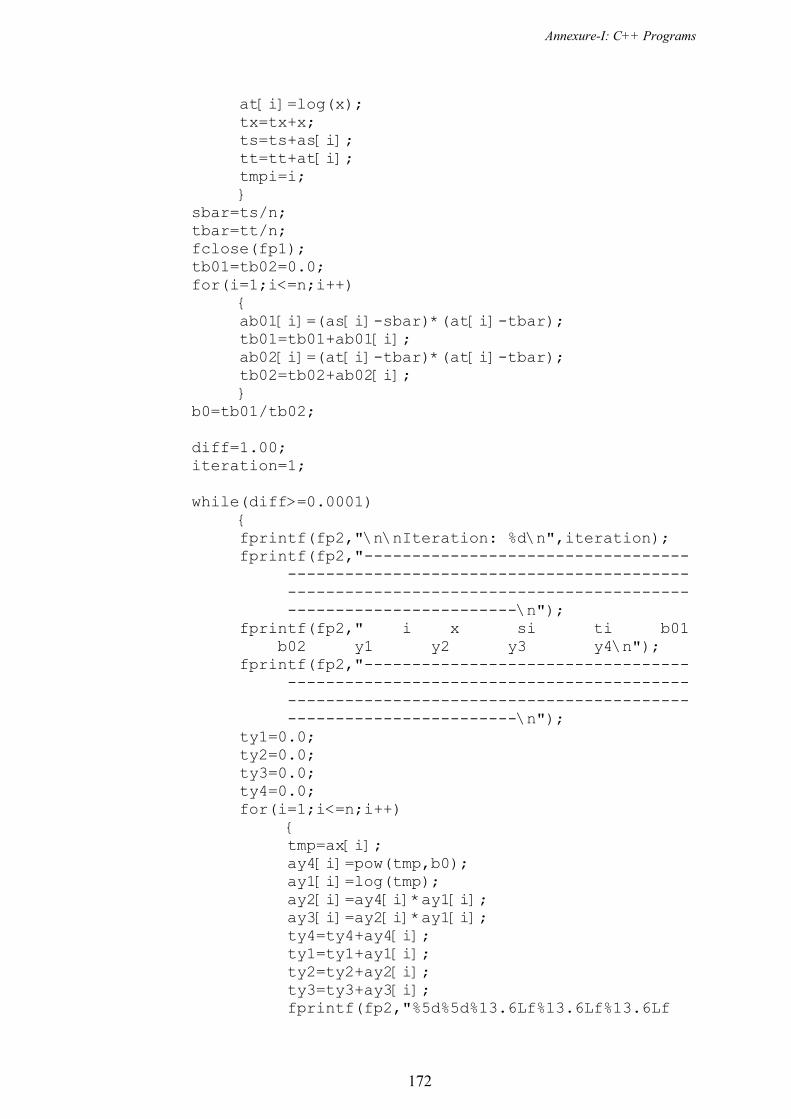
Annexure-I: C++ Programs
172
at[i]=log(x); tx=tx+x; ts=ts+as[i]; tt=tt+at[i]; tmpi=i; } sbar=ts/n; tbar=tt/n; fclose(fp1); tb01=tb02=0.0; for(i=1;i<=n;i++) { ab01[i]=(as[i]-sbar)*(at[i]-tbar); tb01=tb01+ab01[i]; ab02[i]=(at[i]-tbar)*(at[i]-tbar); tb02=tb02+ab02[i]; } b0=tb01/tb02; diff=1.00; iteration=1; while(diff>=0.0001) { fprintf(fp2,"\n\nIteration: %d\n",iteration); fprintf(fp2,"---------------------------------- ------------------------------------------ ------------------------------------------ ------------------------\n"); fprintf(fp2," i x si ti b01
b02 y1 y2 y3 y4\n"); fprintf(fp2,"---------------------------------- ------------------------------------------ ------------------------------------------ ------------------------\n"); ty1=0.0; ty2=0.0; ty3=0.0; ty4=0.0; for(i=1;i<=n;i++) { tmp=ax[i]; ay4[i]=pow(tmp,b0); ay1[i]=log(tmp); ay2[i]=ay4[i]*ay1[i]; ay3[i]=ay2[i]*ay1[i]; ty4=ty4+ay4[i]; ty1=ty1+ay1[i]; ty2=ty2+ay2[i]; ty3=ty3+ay3[i]; fprintf(fp2,"%5d%5d%13.6Lf%13.6Lf%13.6Lf
Annexure-I: C++ Programs
173
%13.6Lf%20.6Lf%20.6Lf%20.6Lf %20.6Lf\n",i,ax[i],as[i],at[i], ab01[i],ab02[i], ay1[i], ay2[i],ay3[i],ay4[i]);
} fprintf(fp2,"---------------------------------- ------------------------------------------ ------------------------------------------ ------------------------\n"); fprintf(fp2,"TOT %5d%13.6Lf%13.6Lf%13.6Lf
%13.6Lf%20.6Lf%20.6Lf%20.6Lf%20.6Lf\n", tx,ts,tt,tb01,tb02,ty1,ty2,ty3,ty4);
fprintf(fp2,"---------------------------------- ------------------------------------------ ------------------------------------------ ------------------------\n"); fprintf(fp2," %13.6Lf%13.6Lf\n",
sbar,tbar); fprintf(fp2,"---------------------------------- ------------------------------------------ ------------------------------------------ ------------------------\n"); t0=ty4/(long double)n; z1=((long double)n/b0)+ty1-(ty2/t0); z2=(-n/pow(b0,2))-(n*ty3/ty4); b1=b0-z1/z2; diff=fabs(b1-b0); fprintf(fp2,"\nb0=%10.7Lf b1=%10.7Lf
difference=%10.7Lf theta= %17.6Lf\n", b0,b1,diff,t0);
b0=b1; iteration++; } fclose(fp2); } 24. gramt.cpp #include <stdio.h> #include <conio.h> #include <math.h> void main() { FILE *fp1,*fp2; long double ts,tt,sbar,tbar,tmp; long double t0,b0,tb01,tb02; long double as[366],at[366],ab01[366],ab02[366]; long double ay4[366],ty4,x,ax[366],tx; /* double tmp;*/ int i,n=365,tmpi; clrscr();
Annexure-I: C++ Programs
174
fp1=fopen("snramta.csv","r"); fp2=fopen("graphamt.txt","w"); if(fp1==NULL) { puts("cannot open the file"); } tmpi=0; tx=0; ts=0.0; tt=0.0; while(fscanf(fp1,"%d,%Lf",&i,&x)!=EOF) { if(tmpi==i) break; ax[i]=x; as[i]=log(log((n+1)/(float)(n-i+1))); at[i]=log(x); tx=tx+x; ts=ts+as[i]; tt=tt+at[i]; tmpi=i; } sbar=ts/n; tbar=tt/n; fclose(fp1); tb01=tb02=0.0; for(i=1;i<=n;i++) { ab01[i]=(as[i]-sbar)*(at[i]-tbar); tb01=tb01+ab01[i]; ab02[i]=(at[i]-tbar)*(at[i]-tbar); tb02=tb02+ab02[i]; } b0=tb01/tb02;
fprintf(fp2,"--------------------------------------- ------------------------------------------ -------------------\n"); fprintf(fp2," i x si ti (si-sbar)(ti-tbar) (ti-tbar)^2 xi^b0\n"); fprintf(fp2,"--------------------------------------- ----------------------------------------------- --------------\n");
ty4=0.0; for(i=1;i<=n;i++) { tmp=ax[i]; ay4[i]=pow(tmp,b0); ty4=ty4+ay4[i];

Annexure-I: C++ Programs
175
fprintf(fp2,"%5d%10.0Lf%13.6Lf%13.6Lf %13.6Lf %13.6Lf %25.6Lf\n", i,ax[i],as[i],at[i],
ab01[i],ab02[i],ay4[i]); } fprintf(fp2,"--------------------------------------- ----------------------------------------------- --------------\n"); fprintf(fp2,"TOT %11.0Lf%13.6Lf%13.6Lf %13.6Lf
%13.6Lf %25.6Lf\n", tx,ts,tt,tb01,tb02,ty4); fprintf(fp2,"--------------------------------------- ----------------------------------------------- --------------\n"); fprintf(fp2," %13.6Lf%13.6Lf\n",sbar,tbar); fprintf(fp2,"--------------------------------------- ----------------------------------------------- --------------\n"); t0=ty4/(long double)n; fprintf(fp2,"\nBeta=%10.7Lf Theta=%17.6Lf\n",
b0,t0); printf("\nBeta=%10.7Lf Theta=%17.6Lf\n",b0,t0); fclose(fp2); getch(); } 25. nramt.cpp #include <stdio.h> #include <conio.h> #include <math.h> void main() { FILE *fp1,*fp2; long double ts,tt,sbar,tbar,tmp; long double z1,z2,t0,b0,b1,diff; long double tb01,tb02,x,ax[366],tx; long double as[366],at[366],ab01[366],ab02[366]; long double ay1[366],ay2[366],ay3[366],ay4[366],
ty1,ty2,ty3,ty4; /* double tmp;*/ int i,n=365,tmpi,iteration=1; clrscr(); fp1=fopen("snramta.csv","r"); fp2=fopen("nramt.txt","w"); if(fp1==NULL) { puts("cannot open the file"); } tmpi=0;
Annexure-I: C++ Programs
176
tx=0; ts=0.0; tt=0.0; while(fscanf(fp1,"%d,%Lf",&i,&x)!=EOF) { if(tmpi==i) break; ax[i]=x; as[i]=log(log((n+1)/(float)(n-i+1))); at[i]=log(x); tx=tx+x; ts=ts+as[i]; tt=tt+at[i]; tmpi=i; } sbar=ts/n; tbar=tt/n; fclose(fp1); tb01=tb02=0.0; for(i=1;i<=n;i++) { ab01[i]=(as[i]-sbar)*(at[i]-tbar); tb01=tb01+ab01[i]; ab02[i]=(at[i]-tbar)*(at[i]-tbar); tb02=tb02+ab02[i]; } b0=tb01/tb02; diff=1.00; iteration=1; while(diff>=0.0001) { fprintf(fp2,"\n\nIteration: %d\n",iteration); fprintf(fp2,"---------------------------------- ------------------------------------------ ------------------------------------------ -------------------------------------\n"); fprintf(fp2," i x si ti b01 b02 y1 y2 y3 y4\n"); fprintf(fp2,"---------------------------------- ------------------------------------------ ------------------------------------------ -------------------------------------\n"); ty1=0.0; ty2=0.0; ty3=0.0; ty4=0.0; for(i=1;i<=n;i++) { tmp=ax[i];
Annexure-I: C++ Programs
177
ay4[i]=pow(tmp,b0); ay1[i]=log(tmp); ay2[i]=ay4[i]*ay1[i]; ay3[i]=ay2[i]*ay1[i]; ty4=ty4+ay4[i]; ty1=ty1+ay1[i]; ty2=ty2+ay2[i]; ty3=ty3+ay3[i]; fprintf(fp2,"%5d%10.0Lf%13.6Lf%13.6Lf
%13.6Lf%13.6Lf%13.6Lf %27.6Lf%27.6Lf %27.6Lf\n",i,ax[i],as[i],at[i],ab01[i],
ab02[i],ay1[i],ay2[i],ay3[i],ay4[i]); } fprintf(fp2,"---------------------------------- ------------------------------------------ ------------------------------------------ -------------------------------------\n"); fprintf(fp2,"TOT %10.0Lf%13.6Lf%13.6Lf%13.6Lf
%13.6Lf%13.6Lf %27.6Lf%27.6Lf%27.6Lf\n", tx,ts,tt,tb01,tb02,ty1,ty2,ty3,ty4);
fprintf(fp2,"---------------------------------- ------------------------------------------ ------------------------------------------ -------------------------------------\n"); fprintf(fp2," %13.6Lf%13.6Lf\n",
sbar,tbar); fprintf(fp2,"---------------------------------- ------------------------------------------ ------------------------------------------ -------------------------------------\n"); t0=ty4/(long double)n; z1=((long double)n/b0)+ty1-(ty2/t0); z2=(-n/pow(b0,2))-(n*ty3/ty4); b1=b0-z1/z2; diff=fabs(b1-b0); fprintf(fp2,"\nb0=%10.7Lf b1=%10.7Lf
difference=%10.7Lf theta=%17.6Lf\n", b0,b1,diff,t0);
b0=b1; iteration++; } fclose(fp2); } 26. anovahit.cpp /* Monthly, Weekly number of hits for time series 1st week- Date 1 to 7 2nd week= Date 8 to 14 3rd week- Date 16 to 21

Annexure-I: C++ Programs
178
Last week- Date 22 to end of the month Generate two dimensional array of hits, Sum ofsquares between months, Sum of squares between weeks, The total sum of square, Error sum of square and ANOVA table, Months as rows and weeks as columns */ #include <stdio.h> # include <conio.h> main() { FILE *fp1; struct atm { int sr; int yy; int mm; int dd; long int dt; double tm; double amt; }; struct atm day; int tmpmm; int i,j,k,hit2[13][5]={{0},{0}},dofr,dofc,dofe; float rtot[13]={0},ctot[5]={0},rtots[13],ctots[5],
gtot,rtotss=0, ctotss=0,hitss=0; float ssr,ssc,cf,sst,sse,msr,msc,mse,
fratior,fratioc; clrscr(); fp1=fopen("ymdtamt.csv","r"); if(fp1==NULL) { puts("cannot open the file"); } i=1; while(fscanf(fp1,"%d,%d,%d,%d,%ld,%lf,%lf",
&day.sr,&day.yy,&day.mm,&day.dd,&day.dt, &day.tm,&day.amt)!=EOF)
{ tmpmm=day.mm; if(day.dd>=1 && day.dd<=7) j=1; if(day.dd>=8 && day.dd<=14) j=2; if(day.dd>=15 && day.dd<=21) j=3; if(day.dd>=22 && day.dd<=31)

Annexure-I: C++ Programs
179
j=4; i=tmpmm; hit2[i][j]++; while(fscanf(fp1,"%d,%d,%d,%d,%ld,%lf,%lf",
&day.sr,&day.yy,&day.mm,&day.dd,&day.dt, &day.tm,&day.amt)!=EOF && tmpmm==day.mm)
{ if(day.dd>=1 && day.dd<=7) j=1; if(day.dd>=8 && day.dd<=14) j=2; if(day.dd>=15 && day.dd<=21) j=3; if(day.dd>=22 && day.dd<=31) j=4; i=tmpmm; hit2[i][j]++; } tmpmm=day.mm; if(day.dd>=1 && day.dd<=7) j=1; if(day.dd>=8 && day.dd<=14) j=2; if(day.dd>=15 && day.dd<=21) j=3; if(day.dd>=22 && day.dd<=31) j=4; i=tmpmm; hit2[i][j]++; } hit2[i][j]--; fclose(fp1); /* TO CALCULATE ROW TOTALS, ITS SQUARES AND SUM OF SQUARES */ for(i=1;i<=12;i++) { for(j=1;j<=4;j++) { rtot[i]=rtot[i]+hit2[i][j]; } rtots[i]=rtot[i]*rtot[i]; rtotss=rtotss+rtots[i]; } /* TO CALCULATE COLUMN TOTALS, ITS SQUARES AND SUM OF SQUARES */ for(j=1;j<=4;j++) { for(i=1;i<=12;i++)

Annexure-I: C++ Programs
180
{ ctot[j]=ctot[j]+hit2[i][j]; } ctots[j]=ctot[j]*ctot[j]; ctotss=ctotss+ctots[j]; } /* TO CALCULATE WEEKLY HITS SUM OF SQUARES (12X4) AND GRAND TOTAL */ for(i=1;i<=12;i++) { for(j=1;j<=4;j++) { hitss=hitss+(float)hit2[i][j]*hit2[i][j]; gtot=gtot+hit2[i][j]; } } /* TO CALCULATE CF, MONTHSS(SSR), HITSS(SSC), TOTAL SS(SST) AND ERROR SS (SSE) */ cf=gtot*gtot/48.0; ssr=rtotss/4-cf; ssc=ctotss/12-cf; sst=hitss-cf; sse=sst-ssr-ssc; printf("\n\n Table showing monthwise weekly hits and sum of squares\n"); printf(" ------------------------------------------- -----------------------------------\n"); printf(" WEEK \n"); printf(" Month I II III Last
Row Sum Sum of square\n"); printf(" ------------------------------------------- -----------------------------------\n"); for(i=1;i<=12;i++) { printf("%5d ",i); for(j=1;j<=4;j++) { printf("%10d",hit2[i][j]); } printf(" %10.2f %10.2f\n",
rtot[i],rtots[i]); } printf(" ------------------------------------------- -----------------------------------\n"); printf(" Column Sum %10.0f%10.0f%10.0f%10.0f %11.2f
%11.2f\n", ctot[1], ctot[2],ctot[3],ctot[4],

Annexure-I: C++ Programs
181
gtot,rtotss); printf(" Sum of Squ. %10.0f%10.0f%10.0f%10.0f
%11.2f\n",ctots[1], ctots[2],ctots[3], ctots[4],ctotss);
printf(" ------------------------------------------- -----------------------------------\n"); printf(" CF = %10.2f Month SS = %10.2f
Week SS = %10.2f\n",cf,ssr,ssc); printf(" Sum of Hit^2 = %10.2f Total SS = %10.2f
Error SS= %10.2f\n",hitss,sst,sse); // printf(" Press any key to continue....\n"); // getch(); // clrscr(); dofr=11; dofc=3; dofe=dofr*dofc; msr=ssr/dofr; msc=ssc/dofc; mse=sse/dofe; fratior=msr/mse; fratioc=msc/mse; printf("\n\n\n The table for Analysis of Variance (ANOVA)\n"); printf(" ------------------------------------------- ------------------------------\n"); printf(" Source of Sum of Degrees of Mean F-Ratios\n"); printf(" variation squares
freedom squares\n"); printf(" ------------------------------------------- ------------------------------\n"); printf(" Between weeks(ssc) %12.2f %2d
%12.2f %12.2f\n\n",ssc,dofc,msc,fratioc); printf(" Between months(ssr)%12.2f %2d
%12.2f %12.2f\n\n", ssr,dofr,msr,fratior); printf(" Error(sse) %12.2f %2d %12.2f\n",sse,dofe,mse); printf(" ------------------------------------------- ------------------------------\n"); getch(); clrscr(); } 27. anovaamt.cpp /* Monthly, Weekly amount withdrawn - ANOVA 1st week- Date 1 to 7 2nd week= Date 8 to 14 3rd week- Date 16 to 21

Annexure-I: C++ Programs
182
Last week- Date 22 to end of the month Generate two dimensional array of hits, Sum ofsquares between months, Sum of squares between weeks, The total sum of square, Error sum of square and ANOVA table, Months as rows and weeks as columns */ #include <stdio.h> # include <conio.h> main() { FILE *fp1; struct atm { int sr; int yy; int mm; int dd; long int dt; double tm; double amt; }; struct atm day; int tmpmm; int i,j,k,dofr,dofc,dofe; double amt2[13][5]={{0},{0}},rtot[13]={0},
ctot[5]={0},rtots[13], ctots[5],gtot, rtotss=0,ctotss=0,amtss=0;
double ssr,ssc,cf,sst,sse,msr,msc,mse, fratior,fratioc;
clrscr(); fp1=fopen("ymdtamt.csv","r"); if(fp1==NULL) { puts("cannot open the file"); } i=1; while(fscanf(fp1,"%d,%d,%d,%d,%ld,%lf,%lf",&day.sr,
&day.yy,&day.mm,&day.dd,&day.dt,&day.tm, &day.amt)!=EOF)
{ tmpmm=day.mm; while(fscanf(fp1,"%d,%d,%d,%d,%ld,%lf,%lf",
&day.sr,&day.yy,&day.mm,&day.dd,&day.dt, &day.tm,&day.amt)!=EOF && tmpmm==day.mm)
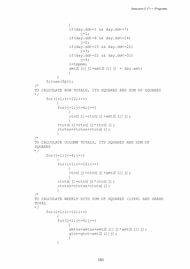
Annexure-I: C++ Programs
183
{ if(day.dd>=1 && day.dd<=7) j=1; if(day.dd>=8 && day.dd<=14) j=2; if(day.dd>=15 && day.dd<=21) j=3; if(day.dd>=22 && day.dd<=31) j=4; i=tmpmm; amt2[i][j]=amt2[i][j] + day.amt; } } fclose(fp1); /* TO CALCULATE ROW TOTALS, ITS SQUARES AND SUM OF SQUARES */ for(i=1;i<=12;i++) { for(j=1;j<=4;j++) { rtot[i]=rtot[i]+amt2[i][j]; } rtots[i]=rtot[i]*rtot[i]; rtotss=rtotss+rtots[i]; } /* TO CALCULATE COLUMN TOTALS, ITS SQUARES AND SUM OF SQUARES */ for(j=1;j<=4;j++) { for(i=1;i<=12;i++) { ctot[j]=ctot[j]+amt2[i][j]; } ctots[j]=ctot[j]*ctot[j]; ctotss=ctotss+ctots[j]; } /* TO CALCULATE WEEKLY HITS SUM OF SQUARES (12X4) AND GRAND TOTAL */ for(i=1;i<=12;i++) { for(j=1;j<=4;j++) { amtss=amtss+amt2[i][j]*amt2[i][j]; gtot=gtot+amt2[i][j]; } }

Annexure-I: C++ Programs
184
/* TO CALCULATE CF, MONTHSS(SSR), HITSS(SSC), TOTAL SS(SST) AND ERROR SS (SSE) */ cf=gtot*gtot/48.0; ssr=rtotss/4-cf; ssc=ctotss/12-cf; sst=amtss-cf; sse=sst-ssr-ssc; printf(" Table showing monthwise amount withdrawn and sum of squares \n"); printf("-------------------------------------------- ----------------------------------\n"); printf(" WEEK \n"); printf("Month I II III Last
Row Sum Row SS\n"); printf("-------------------------------------------- ----------------------------------\n"); for(i=1;i<=12;i++) { printf("%5d ",i); for(j=1;j<=4;j++) { printf("%10.0lf",amt2[i][j]); } printf(" %10.0lf %10.2e\n",rtot[i],rtots[i]); } printf("-------------------------------------------- ----------------------------------\n"); printf("C Sum %10.0lf%10.0lf%10.0lf%10.0lf%11.0lf %10.2e\n",ctot[1],ctot[2],ctot[3],ctot[4],
gtot,rtotss); printf("C SS %10.2e%10.2e%10.2e%10.2e%11.2e\n",
ctots[1], ctots[2],ctots[3],ctots[4],ctotss); printf("-------------------------------------------- ----------------------------------\n"); printf(" CF=%10.0lf Month SS=%10.0lf
Week SS=%10.0lf\n", cf,ssr,ssc); printf("Sum of amt^2=%10.0lf Total SS=%10.0lf Error SS=%10.0lf\n", amtss,sst,sse); printf("Press any key to continue....\n"); getch(); clrscr(); dofr=11; dofc=3; dofe=dofr*dofc;
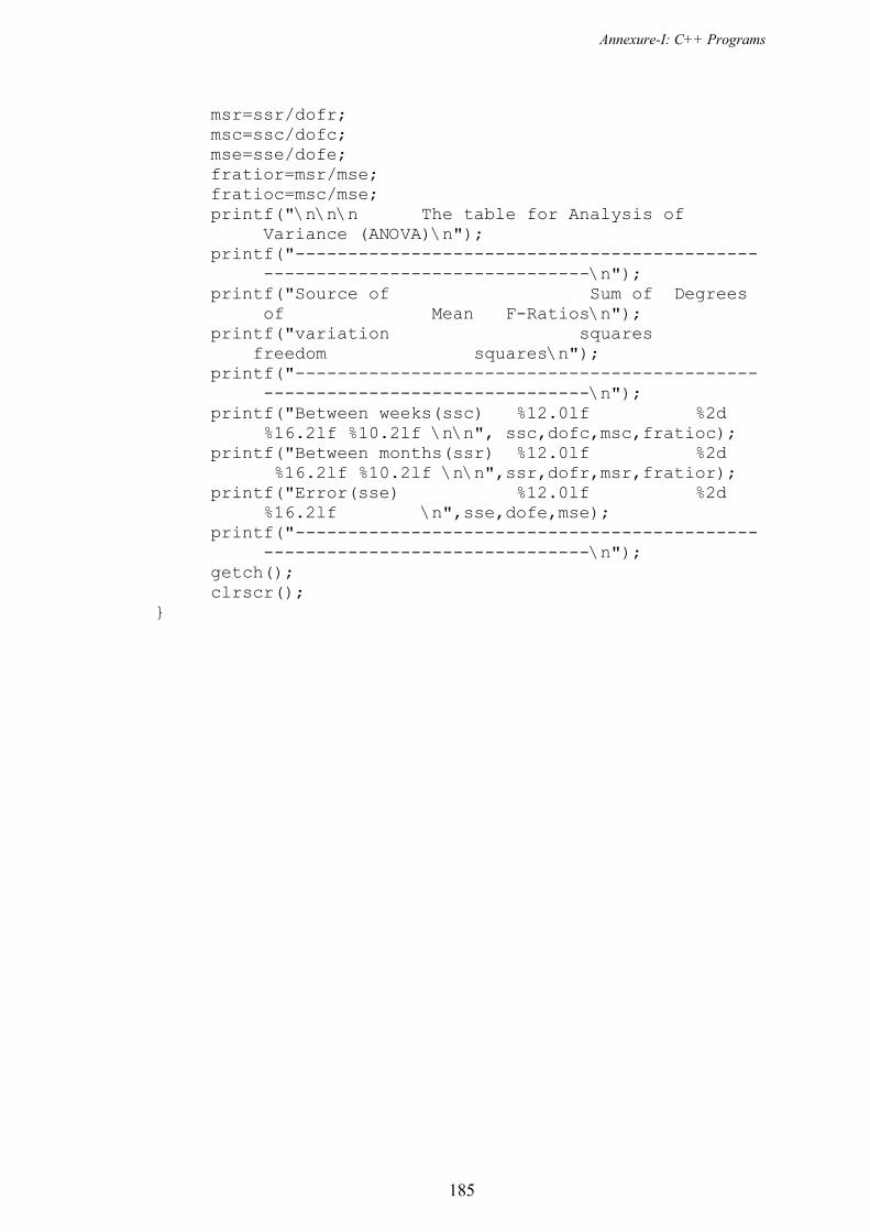
Annexure-I: C++ Programs
185
msr=ssr/dofr; msc=ssc/dofc; mse=sse/dofe; fratior=msr/mse; fratioc=msc/mse; printf("\n\n\n The table for Analysis of Variance (ANOVA)\n"); printf("-------------------------------------------- -------------------------------\n"); printf("Source of Sum of Degrees of Mean F-Ratios\n"); printf("variation squares
freedom squares\n"); printf("-------------------------------------------- -------------------------------\n"); printf("Between weeks(ssc) %12.0lf %2d %16.2lf %10.2lf \n\n", ssc,dofc,msc,fratioc); printf("Between months(ssr) %12.0lf %2d
%16.2lf %10.2lf \n\n",ssr,dofr,msr,fratior); printf("Error(sse) %12.0lf %2d %16.2lf \n",sse,dofe,mse); printf("-------------------------------------------- -------------------------------\n"); getch(); clrscr(); }

Annexure-II: ATM data
186
Annexure-II
ATM data
January-2005
Sr. Date Time Amount1 01/01/05 09:13 80002 01/01/05 09:16 10003 01/01/05 10:40 1004 01/01/05 11:23 100005 01/01/05 11:37 170006 01/01/05 11:50 5007 01/01/05 11:59 3008 01/01/05 12:24 60009 01/01/05 12:35 1200
10 01/01/05 12:36 1000011 01/01/05 12:54 100012 01/01/05 13:44 800013 01/01/05 13:52 250014 01/01/05 14:09 550015 01/01/05 14:20 200016 01/01/05 14:28 430017 01/01/05 14:43 20018 01/01/05 15:28 10019 01/01/05 16:39 100020 01/01/05 16:42 750021 01/01/05 16:45 500022 01/01/05 16:46 20023 01/01/05 17:02 300024 01/01/05 18:01 10025 01/01/05 18:15 20026 01/01/05 18:17 210027 01/01/05 18:19 250028 01/01/05 18:24 300029 01/01/05 18:56 700030 01/01/05 19:11 100031 01/01/05 19:16 2000
32 01/01/05 19:20 200033 01/01/05 19:28 50034 01/01/05 19:29 10035 01/01/05 20:02 10036 01/01/05 20:13 500037 01/01/05 20:55 440038 01/01/05 21:18 620039 01/01/05 21:47 80040 01/01/05 22:04 250041 01/01/05 22:05 300042 01/01/05 23:00 10043 02/01/05 09:08 100044 02/01/05 09:41 200045 02/01/05 10:32 100046 02/01/05 11:06 300047 02/01/05 11:07 100048 02/01/05 11:27 2000049 02/01/05 11:29 100050 02/01/05 11:34 20051 02/01/05 11:44 20052 02/01/05 11:45 20053 02/01/05 12:23 10054 02/01/05 12:33 40055 02/01/05 13:47 50056 02/01/05 13:50 490057 02/01/05 13:52 60058 02/01/05 13:56 100059 02/01/05 14:52 300060 02/01/05 16:34 500061 02/01/05 17:44 140062 02/01/05 17:45 60063 02/01/05 17:48 2500
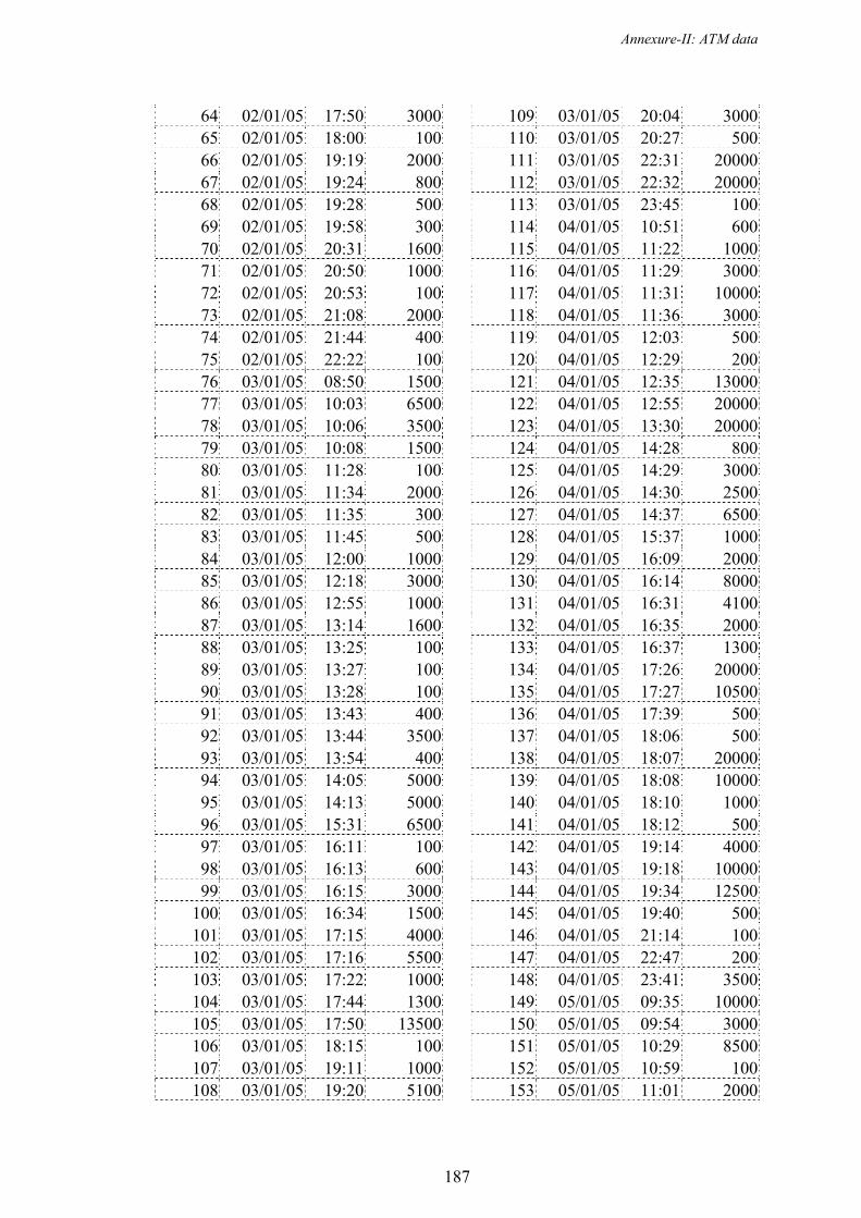
Annexure-II: ATM data
187
64 02/01/05 17:50 300065 02/01/05 18:00 10066 02/01/05 19:19 200067 02/01/05 19:24 80068 02/01/05 19:28 50069 02/01/05 19:58 30070 02/01/05 20:31 160071 02/01/05 20:50 100072 02/01/05 20:53 10073 02/01/05 21:08 200074 02/01/05 21:44 40075 02/01/05 22:22 10076 03/01/05 08:50 150077 03/01/05 10:03 650078 03/01/05 10:06 350079 03/01/05 10:08 150080 03/01/05 11:28 10081 03/01/05 11:34 200082 03/01/05 11:35 30083 03/01/05 11:45 50084 03/01/05 12:00 100085 03/01/05 12:18 300086 03/01/05 12:55 100087 03/01/05 13:14 160088 03/01/05 13:25 10089 03/01/05 13:27 10090 03/01/05 13:28 10091 03/01/05 13:43 40092 03/01/05 13:44 350093 03/01/05 13:54 40094 03/01/05 14:05 500095 03/01/05 14:13 500096 03/01/05 15:31 650097 03/01/05 16:11 10098 03/01/05 16:13 60099 03/01/05 16:15 3000
100 03/01/05 16:34 1500101 03/01/05 17:15 4000102 03/01/05 17:16 5500103 03/01/05 17:22 1000104 03/01/05 17:44 1300105 03/01/05 17:50 13500106 03/01/05 18:15 100107 03/01/05 19:11 1000108 03/01/05 19:20 5100
109 03/01/05 20:04 3000110 03/01/05 20:27 500111 03/01/05 22:31 20000112 03/01/05 22:32 20000113 03/01/05 23:45 100114 04/01/05 10:51 600115 04/01/05 11:22 1000116 04/01/05 11:29 3000117 04/01/05 11:31 10000118 04/01/05 11:36 3000119 04/01/05 12:03 500120 04/01/05 12:29 200121 04/01/05 12:35 13000122 04/01/05 12:55 20000123 04/01/05 13:30 20000124 04/01/05 14:28 800125 04/01/05 14:29 3000126 04/01/05 14:30 2500127 04/01/05 14:37 6500128 04/01/05 15:37 1000129 04/01/05 16:09 2000130 04/01/05 16:14 8000131 04/01/05 16:31 4100132 04/01/05 16:35 2000133 04/01/05 16:37 1300134 04/01/05 17:26 20000135 04/01/05 17:27 10500136 04/01/05 17:39 500137 04/01/05 18:06 500138 04/01/05 18:07 20000139 04/01/05 18:08 10000140 04/01/05 18:10 1000141 04/01/05 18:12 500142 04/01/05 19:14 4000143 04/01/05 19:18 10000144 04/01/05 19:34 12500145 04/01/05 19:40 500146 04/01/05 21:14 100147 04/01/05 22:47 200148 04/01/05 23:41 3500149 05/01/05 09:35 10000150 05/01/05 09:54 3000151 05/01/05 10:29 8500152 05/01/05 10:59 100153 05/01/05 11:01 2000

Annexure-II: ATM data
188
154 05/01/05 12:07 100155 05/01/05 12:59 500156 05/01/05 13:44 1000157 05/01/05 13:45 1000158 05/01/05 14:19 700159 05/01/05 14:45 14000160 05/01/05 15:02 20000161 05/01/05 15:03 20000162 05/01/05 15:34 5000163 05/01/05 16:29 500164 05/01/05 16:36 2000165 05/01/05 17:08 500166 05/01/05 18:00 10000167 05/01/05 18:05 500168 05/01/05 18:06 3000169 05/01/05 18:08 100170 05/01/05 18:16 3000171 05/01/05 18:25 500172 05/01/05 18:30 6000173 05/01/05 19:34 10000174 05/01/05 19:39 2000175 05/01/05 19:44 10300176 05/01/05 19:45 100177 05/01/05 20:19 100178 05/01/05 20:20 100179 05/01/05 20:59 2500180 05/01/05 22:38 3000181 06/01/05 09:39 8500182 06/01/05 09:40 500183 06/01/05 09:45 4500184 06/01/05 09:45 4500185 06/01/05 11:29 10000186 06/01/05 11:33 200187 06/01/05 11:51 100188 06/01/05 12:43 500189 06/01/05 12:57 1100190 06/01/05 13:01 200191 06/01/05 13:22 200192 06/01/05 13:24 5000193 06/01/05 13:26 13000194 06/01/05 13:37 500195 06/01/05 14:45 20000196 06/01/05 15:06 3000197 06/01/05 15:31 1000198 06/01/05 15:35 20000
199 06/01/05 16:34 3100200 06/01/05 16:37 4000201 06/01/05 17:07 10000202 06/01/05 17:22 200203 06/01/05 18:26 3000204 06/01/05 18:30 3000205 06/01/05 18:31 2000206 06/01/05 18:41 500207 06/01/05 18:48 300208 06/01/05 19:00 1100209 06/01/05 19:15 1000210 06/01/05 19:27 20000211 06/01/05 20:08 100212 06/01/05 21:58 1000213 06/01/05 22:01 10000214 07/01/05 10:55 4300215 07/01/05 10:56 6000216 07/01/05 10:57 300217 07/01/05 10:59 10000218 07/01/05 11:21 6000219 07/01/05 11:34 300220 07/01/05 11:45 3000221 07/01/05 11:45 2000222 07/01/05 11:47 500223 07/01/05 11:50 600224 07/01/05 12:02 600225 07/01/05 12:14 1000226 07/01/05 12:31 15000227 07/01/05 12:34 1200228 07/01/05 12:55 2000229 07/01/05 13:34 10000230 07/01/05 14:16 7000231 07/01/05 14:19 20000232 07/01/05 15:49 500233 07/01/05 18:14 400234 07/01/05 18:16 9000235 07/01/05 18:27 600236 07/01/05 18:50 300237 07/01/05 18:57 3600238 07/01/05 19:09 2900239 07/01/05 19:36 100240 07/01/05 19:51 200241 07/01/05 20:00 700242 07/01/05 21:44 1000243 08/01/05 11:04 20000
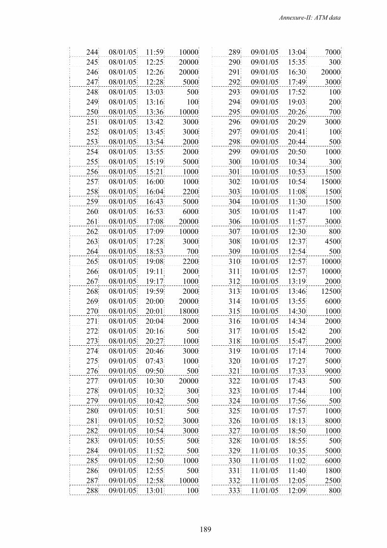
Annexure-II: ATM data
189
244 08/01/05 11:59 10000245 08/01/05 12:25 20000246 08/01/05 12:26 20000247 08/01/05 12:28 5000248 08/01/05 13:03 500249 08/01/05 13:16 100250 08/01/05 13:36 10000251 08/01/05 13:42 3000252 08/01/05 13:45 3000253 08/01/05 13:54 2000254 08/01/05 13:55 2000255 08/01/05 15:19 5000256 08/01/05 15:21 1000257 08/01/05 16:00 1000258 08/01/05 16:04 2200259 08/01/05 16:43 5000260 08/01/05 16:53 6000261 08/01/05 17:08 20000262 08/01/05 17:09 10000263 08/01/05 17:28 3000264 08/01/05 18:53 700265 08/01/05 19:08 2200266 08/01/05 19:11 2000267 08/01/05 19:17 1000268 08/01/05 19:59 2000269 08/01/05 20:00 20000270 08/01/05 20:01 18000271 08/01/05 20:04 2000272 08/01/05 20:16 500273 08/01/05 20:27 1000274 08/01/05 20:46 3000275 09/01/05 07:43 1000276 09/01/05 09:50 500277 09/01/05 10:30 20000278 09/01/05 10:32 300279 09/01/05 10:42 500280 09/01/05 10:51 500281 09/01/05 10:52 3000282 09/01/05 10:54 3000283 09/01/05 10:55 500284 09/01/05 11:52 500285 09/01/05 12:50 1000286 09/01/05 12:55 500287 09/01/05 12:58 10000288 09/01/05 13:01 100
289 09/01/05 13:04 7000290 09/01/05 15:35 300291 09/01/05 16:30 20000292 09/01/05 17:49 3000293 09/01/05 17:52 100294 09/01/05 19:03 200295 09/01/05 20:26 700296 09/01/05 20:29 3000297 09/01/05 20:41 100298 09/01/05 20:44 500299 09/01/05 20:50 1000300 10/01/05 10:34 300301 10/01/05 10:53 1500302 10/01/05 10:54 15000303 10/01/05 11:08 1500304 10/01/05 11:30 1500305 10/01/05 11:47 100306 10/01/05 11:57 3000307 10/01/05 12:30 800308 10/01/05 12:37 4500309 10/01/05 12:54 500310 10/01/05 12:57 10000311 10/01/05 12:57 10000312 10/01/05 13:19 2000313 10/01/05 13:46 12500314 10/01/05 13:55 6000315 10/01/05 14:30 1000316 10/01/05 14:34 2000317 10/01/05 15:42 200318 10/01/05 15:47 2000319 10/01/05 17:14 7000320 10/01/05 17:27 5000321 10/01/05 17:33 9000322 10/01/05 17:43 500323 10/01/05 17:44 100324 10/01/05 17:56 500325 10/01/05 17:57 1000326 10/01/05 18:13 8000327 10/01/05 18:50 1000328 10/01/05 18:55 500329 11/01/05 10:35 5000330 11/01/05 11:02 6000331 11/01/05 11:40 1800332 11/01/05 12:05 2500333 11/01/05 12:09 800

Annexure-II: ATM data
190
334 11/01/05 12:13 1000335 11/01/05 12:14 100336 11/01/05 12:17 3000337 11/01/05 12:25 13000338 11/01/05 12:37 7000339 11/01/05 12:56 11000340 11/01/05 12:57 4000341 11/01/05 13:00 500342 11/01/05 13:11 800343 11/01/05 13:18 20000344 11/01/05 13:19 10000345 11/01/05 13:40 500346 11/01/05 14:02 3000347 11/01/05 14:17 300348 11/01/05 15:06 300349 11/01/05 15:13 10000350 11/01/05 15:39 10000351 11/01/05 15:40 5000352 11/01/05 15:41 5000353 11/01/05 16:26 1000354 11/01/05 16:57 500355 11/01/05 17:06 2500356 11/01/05 17:57 1000357 11/01/05 18:16 1500358 11/01/05 18:39 1200359 11/01/05 18:50 600360 11/01/05 18:55 3000361 11/01/05 18:58 100362 11/01/05 19:24 3000363 11/01/05 21:37 5000364 11/01/05 22:09 3000365 12/01/05 09:07 500366 12/01/05 09:12 300367 12/01/05 10:09 100368 12/01/05 10:30 300369 12/01/05 10:57 300370 12/01/05 11:23 5000371 12/01/05 11:26 10000372 12/01/05 11:37 500373 12/01/05 11:38 500374 12/01/05 11:39 500375 12/01/05 11:40 500376 12/01/05 11:41 500377 12/01/05 11:42 500378 12/01/05 11:45 500
379 12/01/05 11:48 1000380 12/01/05 11:58 2000381 12/01/05 12:28 20000382 12/01/05 12:38 100383 12/01/05 12:46 3700384 12/01/05 14:09 400385 12/01/05 14:37 3000386 12/01/05 14:53 20000387 12/01/05 14:54 5000388 12/01/05 14:56 1000389 12/01/05 15:01 3000390 12/01/05 15:12 700391 12/01/05 15:15 8000392 12/01/05 15:30 18000393 12/01/05 15:57 3000394 12/01/05 16:33 100395 12/01/05 16:36 100396 12/01/05 16:58 500397 12/01/05 17:04 10000398 12/01/05 17:21 12000399 12/01/05 17:26 200400 12/01/05 17:30 3000401 12/01/05 18:14 500402 12/01/05 19:08 200403 12/01/05 19:41 2500404 12/01/05 20:07 800405 12/01/05 20:32 1000406 12/01/05 20:33 500407 12/01/05 21:21 4000408 12/01/05 21:51 6100409 12/01/05 22:31 1000410 13/01/05 08:24 700411 13/01/05 10:23 10000412 13/01/05 11:11 17000413 13/01/05 11:21 8000414 13/01/05 11:30 10000415 13/01/05 11:46 500416 13/01/05 11:50 1000417 13/01/05 11:54 500418 13/01/05 11:57 500419 13/01/05 12:11 600420 13/01/05 12:12 20000421 13/01/05 12:13 10000422 13/01/05 12:19 20000423 13/01/05 12:24 10000

Annexure-II: ATM data
191
424 13/01/05 12:38 14000425 13/01/05 12:41 1000426 13/01/05 12:44 3000427 13/01/05 13:00 500428 13/01/05 13:18 3000429 13/01/05 13:33 3000430 13/01/05 13:38 700431 13/01/05 13:41 100432 13/01/05 13:57 100433 13/01/05 15:13 20000434 13/01/05 15:14 10000435 13/01/05 15:19 1500436 13/01/05 15:44 2000437 13/01/05 16:20 3000438 13/01/05 17:43 500439 13/01/05 17:46 1000440 13/01/05 17:54 500441 13/01/05 17:57 500442 13/01/05 18:12 3500443 13/01/05 18:27 3000444 13/01/05 18:27 3000445 13/01/05 18:35 10000446 13/01/05 18:37 300447 13/01/05 19:01 500448 13/01/05 19:13 100449 13/01/05 19:35 200450 13/01/05 19:54 1000451 13/01/05 20:04 100452 13/01/05 20:44 100453 14/01/05 09:45 400454 14/01/05 10:11 2700455 14/01/05 10:46 1000456 14/01/05 11:35 1000457 14/01/05 12:33 5000458 14/01/05 12:49 2500459 14/01/05 13:07 200460 14/01/05 13:09 300461 14/01/05 13:26 2000462 14/01/05 13:30 500463 14/01/05 13:59 3000464 14/01/05 14:01 3000465 14/01/05 14:02 1000466 14/01/05 15:01 600467 14/01/05 15:05 300468 14/01/05 16:10 500
469 14/01/05 16:16 300470 14/01/05 16:27 200471 14/01/05 19:37 5000472 14/01/05 21:00 1000473 14/01/05 21:03 100474 14/01/05 21:33 200475 14/01/05 23:03 5000476 15/01/05 08:57 2800477 15/01/05 08:58 5000478 15/01/05 09:50 5000479 15/01/05 09:59 300480 15/01/05 10:00 10000481 15/01/05 10:14 2000482 15/01/05 11:29 1500483 15/01/05 11:32 5000484 15/01/05 11:49 5000485 15/01/05 12:46 200486 15/01/05 13:08 18000487 15/01/05 13:23 300488 15/01/05 13:49 5500489 15/01/05 14:29 15000490 15/01/05 15:18 900491 15/01/05 16:12 700492 15/01/05 16:29 300493 15/01/05 17:22 1500494 15/01/05 17:25 2000495 15/01/05 17:27 300496 15/01/05 17:50 600497 15/01/05 18:06 200498 15/01/05 18:09 20000499 15/01/05 18:10 5000500 15/01/05 18:31 200501 15/01/05 18:59 500502 15/01/05 19:45 3000503 15/01/05 19:59 600504 15/01/05 20:14 2500505 15/01/05 21:46 3600506 16/01/05 10:31 2000507 16/01/05 10:35 3000508 16/01/05 11:06 1000509 16/01/05 11:08 300510 16/01/05 11:56 1500511 16/01/05 11:59 1000512 16/01/05 12:21 1000513 16/01/05 13:07 100

Annexure-II: ATM data
192
514 16/01/05 13:30 2000515 16/01/05 17:30 1000516 16/01/05 18:34 2000517 16/01/05 18:47 1000518 16/01/05 19:02 500519 16/01/05 19:22 500520 16/01/05 21:55 100521 17/01/05 09:12 2700522 17/01/05 09:37 100523 17/01/05 10:55 100524 17/01/05 11:12 500525 17/01/05 11:40 20000526 17/01/05 11:52 2000527 17/01/05 11:59 1000528 17/01/05 12:04 18000529 17/01/05 12:05 1000530 17/01/05 12:19 500531 17/01/05 12:58 500532 17/01/05 13:57 400533 17/01/05 14:20 2500534 17/01/05 15:06 20000535 17/01/05 15:08 6000536 17/01/05 15:10 10000537 17/01/05 15:11 200538 17/01/05 15:48 20000539 17/01/05 16:35 1000540 17/01/05 17:03 2500541 17/01/05 17:30 10000542 17/01/05 17:32 10500543 17/01/05 17:52 20000544 17/01/05 17:54 14500545 17/01/05 18:13 1000546 17/01/05 18:14 300547 17/01/05 18:40 600548 17/01/05 18:43 2000549 17/01/05 19:08 100550 17/01/05 19:11 500551 17/01/05 19:19 1000552 17/01/05 19:25 600553 17/01/05 20:19 1000554 17/01/05 20:21 1000555 17/01/05 20:23 1000556 17/01/05 20:25 1000557 17/01/05 20:32 1000558 17/01/05 20:36 8000
559 18/01/05 09:05 3000560 18/01/05 09:06 3000561 18/01/05 09:14 2000562 18/01/05 10:11 2000563 18/01/05 10:28 2400564 18/01/05 13:15 1000565 18/01/05 13:21 200566 18/01/05 13:36 15000567 18/01/05 14:08 2500568 18/01/05 14:10 500569 18/01/05 14:11 3000570 18/01/05 14:18 4500571 18/01/05 14:26 3000572 18/01/05 14:39 10500573 18/01/05 15:44 100574 18/01/05 15:45 100575 18/01/05 16:07 10000576 18/01/05 16:18 3000577 18/01/05 16:21 3000578 18/01/05 16:22 3000579 18/01/05 16:23 3000580 18/01/05 16:24 3000581 18/01/05 16:25 3000582 18/01/05 16:26 1000583 18/01/05 16:36 1500584 18/01/05 16:40 3000585 18/01/05 16:41 2000586 18/01/05 16:50 2000587 18/01/05 17:29 10000588 18/01/05 17:46 400589 18/01/05 17:56 500590 18/01/05 18:27 6000591 18/01/05 18:30 300592 18/01/05 18:39 100593 18/01/05 21:15 500594 19/01/05 09:56 100595 19/01/05 10:45 500596 19/01/05 11:23 2000597 19/01/05 11:27 11000598 19/01/05 11:53 21000599 19/01/05 12:03 1000600 19/01/05 12:10 1000601 19/01/05 12:16 1300602 19/01/05 12:18 2000603 19/01/05 12:20 200
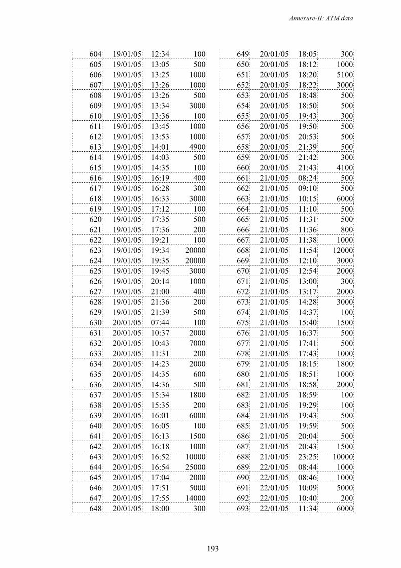
Annexure-II: ATM data
193
604 19/01/05 12:34 100605 19/01/05 13:05 500606 19/01/05 13:25 1000607 19/01/05 13:26 1000608 19/01/05 13:26 500609 19/01/05 13:34 3000610 19/01/05 13:36 100611 19/01/05 13:45 1000612 19/01/05 13:53 1000613 19/01/05 14:01 4900614 19/01/05 14:03 500615 19/01/05 14:35 100616 19/01/05 16:19 400617 19/01/05 16:28 300618 19/01/05 16:33 3000619 19/01/05 17:12 100620 19/01/05 17:35 500621 19/01/05 17:36 200622 19/01/05 19:21 100623 19/01/05 19:34 20000624 19/01/05 19:35 20000625 19/01/05 19:45 3000626 19/01/05 20:14 1000627 19/01/05 21:00 400628 19/01/05 21:36 200629 19/01/05 21:39 500630 20/01/05 07:44 100631 20/01/05 10:37 2000632 20/01/05 10:43 7000633 20/01/05 11:31 200634 20/01/05 14:23 2000635 20/01/05 14:35 600636 20/01/05 14:36 500637 20/01/05 15:34 1800638 20/01/05 15:35 200639 20/01/05 16:01 6000640 20/01/05 16:05 100641 20/01/05 16:13 1500642 20/01/05 16:18 1000643 20/01/05 16:52 10000644 20/01/05 16:54 25000645 20/01/05 17:04 2000646 20/01/05 17:51 5000647 20/01/05 17:55 14000648 20/01/05 18:00 300
649 20/01/05 18:05 300650 20/01/05 18:12 1000651 20/01/05 18:20 5100652 20/01/05 18:22 3000653 20/01/05 18:48 500654 20/01/05 18:50 500655 20/01/05 19:43 300656 20/01/05 19:50 500657 20/01/05 20:53 500658 20/01/05 21:39 500659 20/01/05 21:42 300660 20/01/05 21:43 4100661 21/01/05 08:24 500662 21/01/05 09:10 500663 21/01/05 10:15 6000664 21/01/05 11:10 500665 21/01/05 11:31 500666 21/01/05 11:36 800667 21/01/05 11:38 1000668 21/01/05 11:54 12000669 21/01/05 12:10 3000670 21/01/05 12:54 2000671 21/01/05 13:00 300672 21/01/05 13:17 2000673 21/01/05 14:28 3000674 21/01/05 14:37 100675 21/01/05 15:40 1500676 21/01/05 16:37 500677 21/01/05 17:41 500678 21/01/05 17:43 1000679 21/01/05 18:15 1800680 21/01/05 18:51 1000681 21/01/05 18:58 2000682 21/01/05 18:59 100683 21/01/05 19:29 100684 21/01/05 19:43 500685 21/01/05 19:59 500686 21/01/05 20:04 500687 21/01/05 20:43 1500688 21/01/05 23:25 10000689 22/01/05 08:44 1000690 22/01/05 08:46 1000691 22/01/05 10:09 5000692 22/01/05 10:40 200693 22/01/05 11:34 6000
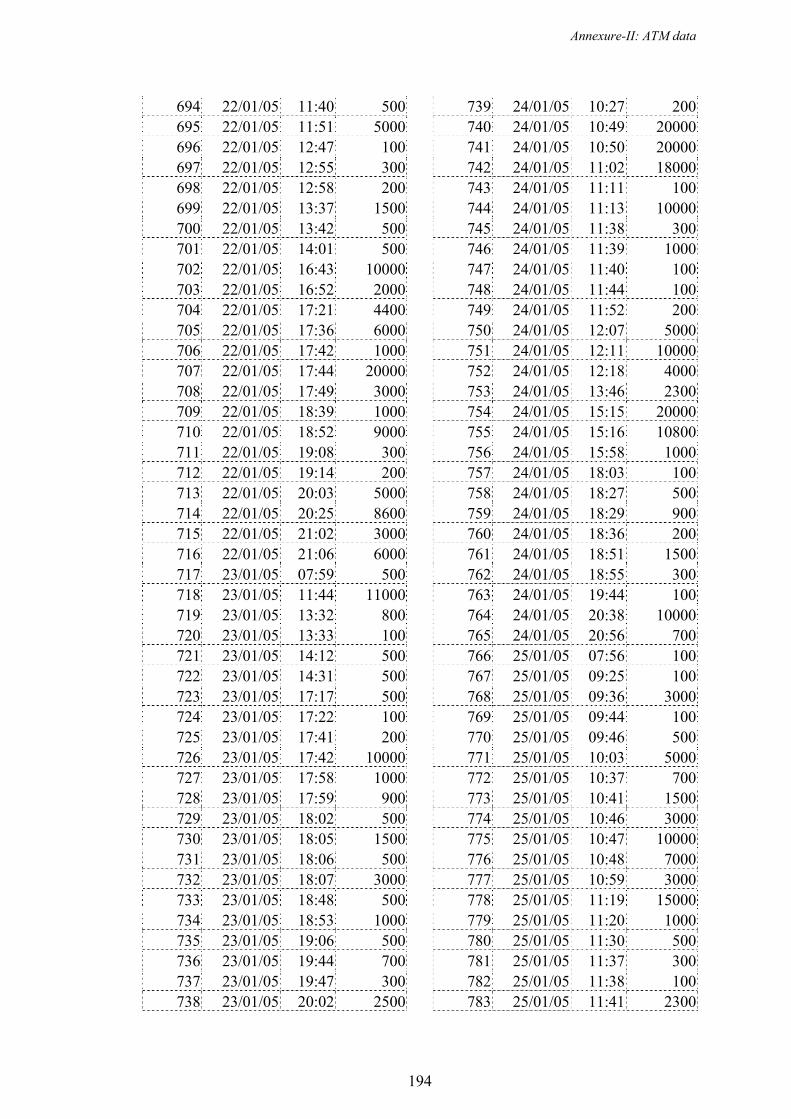
Annexure-II: ATM data
194
694 22/01/05 11:40 500695 22/01/05 11:51 5000696 22/01/05 12:47 100697 22/01/05 12:55 300698 22/01/05 12:58 200699 22/01/05 13:37 1500700 22/01/05 13:42 500701 22/01/05 14:01 500702 22/01/05 16:43 10000703 22/01/05 16:52 2000704 22/01/05 17:21 4400705 22/01/05 17:36 6000706 22/01/05 17:42 1000707 22/01/05 17:44 20000708 22/01/05 17:49 3000709 22/01/05 18:39 1000710 22/01/05 18:52 9000711 22/01/05 19:08 300712 22/01/05 19:14 200713 22/01/05 20:03 5000714 22/01/05 20:25 8600715 22/01/05 21:02 3000716 22/01/05 21:06 6000717 23/01/05 07:59 500718 23/01/05 11:44 11000719 23/01/05 13:32 800720 23/01/05 13:33 100721 23/01/05 14:12 500722 23/01/05 14:31 500723 23/01/05 17:17 500724 23/01/05 17:22 100725 23/01/05 17:41 200726 23/01/05 17:42 10000727 23/01/05 17:58 1000728 23/01/05 17:59 900729 23/01/05 18:02 500730 23/01/05 18:05 1500731 23/01/05 18:06 500732 23/01/05 18:07 3000733 23/01/05 18:48 500734 23/01/05 18:53 1000735 23/01/05 19:06 500736 23/01/05 19:44 700737 23/01/05 19:47 300738 23/01/05 20:02 2500
739 24/01/05 10:27 200740 24/01/05 10:49 20000741 24/01/05 10:50 20000742 24/01/05 11:02 18000743 24/01/05 11:11 100744 24/01/05 11:13 10000745 24/01/05 11:38 300746 24/01/05 11:39 1000747 24/01/05 11:40 100748 24/01/05 11:44 100749 24/01/05 11:52 200750 24/01/05 12:07 5000751 24/01/05 12:11 10000752 24/01/05 12:18 4000753 24/01/05 13:46 2300754 24/01/05 15:15 20000755 24/01/05 15:16 10800756 24/01/05 15:58 1000757 24/01/05 18:03 100758 24/01/05 18:27 500759 24/01/05 18:29 900760 24/01/05 18:36 200761 24/01/05 18:51 1500762 24/01/05 18:55 300763 24/01/05 19:44 100764 24/01/05 20:38 10000765 24/01/05 20:56 700766 25/01/05 07:56 100767 25/01/05 09:25 100768 25/01/05 09:36 3000769 25/01/05 09:44 100770 25/01/05 09:46 500771 25/01/05 10:03 5000772 25/01/05 10:37 700773 25/01/05 10:41 1500774 25/01/05 10:46 3000775 25/01/05 10:47 10000776 25/01/05 10:48 7000777 25/01/05 10:59 3000778 25/01/05 11:19 15000779 25/01/05 11:20 1000780 25/01/05 11:30 500781 25/01/05 11:37 300782 25/01/05 11:38 100783 25/01/05 11:41 2300
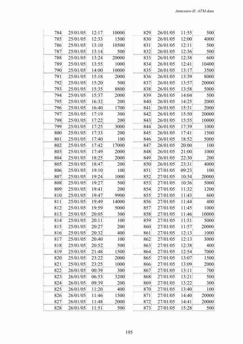
Annexure-II: ATM data
195
784 25/01/05 12:17 10000785 25/01/05 12:33 1500786 25/01/05 13:10 10500787 25/01/05 13:14 500788 25/01/05 13:24 20000789 25/01/05 13:55 1000790 25/01/05 14:00 10000791 25/01/05 15:18 2000792 25/01/05 15:20 500793 25/01/05 15:35 8800794 25/01/05 15:37 2000795 25/01/05 16:32 200796 25/01/05 16:40 1700797 25/01/05 17:19 300798 25/01/05 17:22 200799 25/01/05 17:25 3000800 25/01/05 17:33 200801 25/01/05 17:40 100802 25/01/05 17:42 17000803 25/01/05 17:49 2000804 25/01/05 18:25 2000805 25/01/05 18:47 200806 25/01/05 19:10 100807 25/01/05 19:24 1000808 25/01/05 19:27 500809 25/01/05 19:41 200810 25/01/05 19:47 9900811 25/01/05 19:49 14000812 25/01/05 19:59 5000813 25/01/05 20:05 300814 25/01/05 20:11 100815 25/01/05 20:27 200816 25/01/05 20:32 400817 25/01/05 20:40 100818 25/01/05 20:52 500819 25/01/05 21:48 1500820 25/01/05 23:22 2000821 25/01/05 23:25 1000822 26/01/05 00:39 300823 26/01/05 06:53 3200824 26/01/05 09:39 200825 26/01/05 11:20 400826 26/01/05 11:46 1500827 26/01/05 11:48 2000828 26/01/05 11:51 500
829 26/01/05 11:55 500830 26/01/05 12:00 4000831 26/01/05 12:11 500832 26/01/05 12:36 500833 26/01/05 12:38 600834 26/01/05 12:41 10400835 26/01/05 13:17 3500836 26/01/05 13:39 8000837 26/01/05 13:57 20000838 26/01/05 13:58 5000839 26/01/05 14:04 500840 26/01/05 14:25 2000841 26/01/05 15:31 2000842 26/01/05 15:50 20000843 26/01/05 15:55 10000844 26/01/05 17:39 1000845 26/01/05 17:41 1500846 26/01/05 18:52 5000847 26/01/05 20:00 100848 26/01/05 21:00 1000849 26/01/05 22:30 200850 26/01/05 23:31 4000851 27/01/05 09:23 100852 27/01/05 10:34 20000853 27/01/05 10:36 5000854 27/01/05 11:32 1200855 27/01/05 11:43 600856 27/01/05 11:44 400857 27/01/05 11:45 1000858 27/01/05 11:46 10000859 27/01/05 11:51 5000860 27/01/05 11:57 20000861 27/01/05 12:13 1000862 27/01/05 12:13 3000863 27/01/05 12:38 400864 27/01/05 12:54 7000865 27/01/05 13:07 1500866 27/01/05 13:09 2000867 27/01/05 13:11 700868 27/01/05 13:21 500869 27/01/05 13:22 300870 27/01/05 13:40 100871 27/01/05 14:40 20000872 27/01/05 14:41 20000873 27/01/05 15:28 500
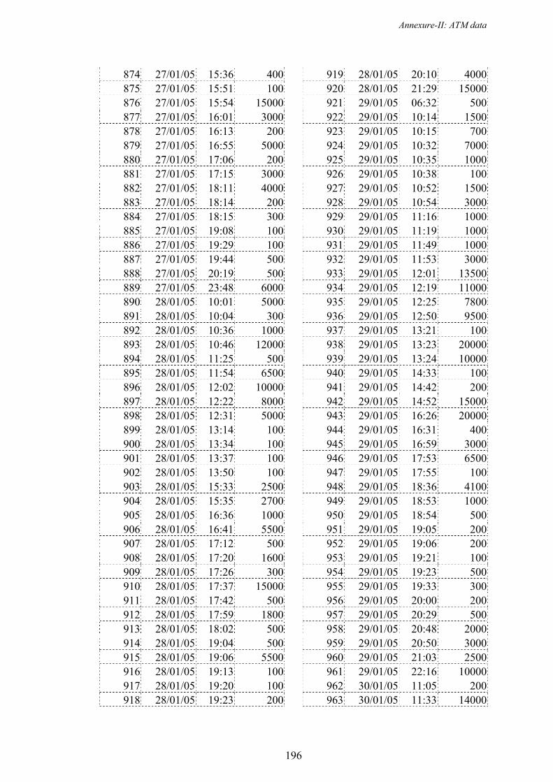
Annexure-II: ATM data
196
874 27/01/05 15:36 400875 27/01/05 15:51 100876 27/01/05 15:54 15000877 27/01/05 16:01 3000878 27/01/05 16:13 200879 27/01/05 16:55 5000880 27/01/05 17:06 200881 27/01/05 17:15 3000882 27/01/05 18:11 4000883 27/01/05 18:14 200884 27/01/05 18:15 300885 27/01/05 19:08 100886 27/01/05 19:29 100887 27/01/05 19:44 500888 27/01/05 20:19 500889 27/01/05 23:48 6000890 28/01/05 10:01 5000891 28/01/05 10:04 300892 28/01/05 10:36 1000893 28/01/05 10:46 12000894 28/01/05 11:25 500895 28/01/05 11:54 6500896 28/01/05 12:02 10000897 28/01/05 12:22 8000898 28/01/05 12:31 5000899 28/01/05 13:14 100900 28/01/05 13:34 100901 28/01/05 13:37 100902 28/01/05 13:50 100903 28/01/05 15:33 2500904 28/01/05 15:35 2700905 28/01/05 16:36 1000906 28/01/05 16:41 5500907 28/01/05 17:12 500908 28/01/05 17:20 1600909 28/01/05 17:26 300910 28/01/05 17:37 15000911 28/01/05 17:42 500912 28/01/05 17:59 1800913 28/01/05 18:02 500914 28/01/05 19:04 500915 28/01/05 19:06 5500916 28/01/05 19:13 100917 28/01/05 19:20 100918 28/01/05 19:23 200
919 28/01/05 20:10 4000920 28/01/05 21:29 15000921 29/01/05 06:32 500922 29/01/05 10:14 1500923 29/01/05 10:15 700924 29/01/05 10:32 7000925 29/01/05 10:35 1000926 29/01/05 10:38 100927 29/01/05 10:52 1500928 29/01/05 10:54 3000929 29/01/05 11:16 1000930 29/01/05 11:19 1000931 29/01/05 11:49 1000932 29/01/05 11:53 3000933 29/01/05 12:01 13500934 29/01/05 12:19 11000935 29/01/05 12:25 7800936 29/01/05 12:50 9500937 29/01/05 13:21 100938 29/01/05 13:23 20000939 29/01/05 13:24 10000940 29/01/05 14:33 100941 29/01/05 14:42 200942 29/01/05 14:52 15000943 29/01/05 16:26 20000944 29/01/05 16:31 400945 29/01/05 16:59 3000946 29/01/05 17:53 6500947 29/01/05 17:55 100948 29/01/05 18:36 4100949 29/01/05 18:53 1000950 29/01/05 18:54 500951 29/01/05 19:05 200952 29/01/05 19:06 200953 29/01/05 19:21 100954 29/01/05 19:23 500955 29/01/05 19:33 300956 29/01/05 20:00 200957 29/01/05 20:29 500958 29/01/05 20:48 2000959 29/01/05 20:50 3000960 29/01/05 21:03 2500961 29/01/05 22:16 10000962 30/01/05 11:05 200963 30/01/05 11:33 14000

Annexure-II: ATM data
197
964 30/01/05 11:50 200965 30/01/05 11:52 500966 30/01/05 11:53 200967 30/01/05 12:45 200968 30/01/05 12:47 9000969 30/01/05 12:50 100970 30/01/05 12:51 1000971 30/01/05 12:56 1400972 30/01/05 15:05 1500973 30/01/05 15:21 100974 30/01/05 15:47 1000975 30/01/05 16:41 500976 30/01/05 17:36 1000977 30/01/05 18:35 300978 30/01/05 18:44 1500979 30/01/05 18:48 300980 30/01/05 19:06 100981 30/01/05 19:08 200982 30/01/05 20:05 100983 30/01/05 20:26 100984 30/01/05 21:11 400985 30/01/05 22:27 10000986 30/01/05 23:35 5000987 30/01/05 23:52 5000988 31/01/05 08:55 100989 31/01/05 09:27 500990 31/01/05 09:35 2000991 31/01/05 09:48 800992 31/01/05 09:51 2500993 31/01/05 09:53 600994 31/01/05 09:58 20000995 31/01/05 10:29 500996 31/01/05 10:33 500997 31/01/05 10:50 10000998 31/01/05 11:02 2500999 31/01/05 11:03 5900
1000 31/01/05 11:29 1001001 31/01/05 11:30 2001002 31/01/05 11:53 20000
1003 31/01/05 12:01 28001004 31/01/05 12:04 100001005 31/01/05 12:09 100001006 31/01/05 12:20 10001007 31/01/05 13:04 200001008 31/01/05 14:09 47001009 31/01/05 14:28 20001010 31/01/05 14:39 20001011 31/01/05 15:25 20001012 31/01/05 15:35 150001013 31/01/05 15:43 20001014 31/01/05 16:08 20001015 31/01/05 16:24 10001016 31/01/05 16:41 10001017 31/01/05 16:42 200001018 31/01/05 16:43 200001019 31/01/05 16:48 2001020 31/01/05 16:49 200001021 31/01/05 16:52 208001022 31/01/05 16:53 52001023 31/01/05 17:22 54001024 31/01/05 17:34 1001025 31/01/05 17:53 9001026 31/01/05 18:14 3001027 31/01/05 18:16 3001028 31/01/05 18:20 50001029 31/01/05 18:21 10001030 31/01/05 18:50 3001031 31/01/05 19:02 4001032 31/01/05 19:10 6001033 31/01/05 19:11 8001034 31/01/05 19:43 50001035 31/01/05 20:01 50001036 31/01/05 20:11 2001037 31/01/05 20:36 25001038 31/01/05 21:49 1001039 31/01/05 21:54 700
.
.
.
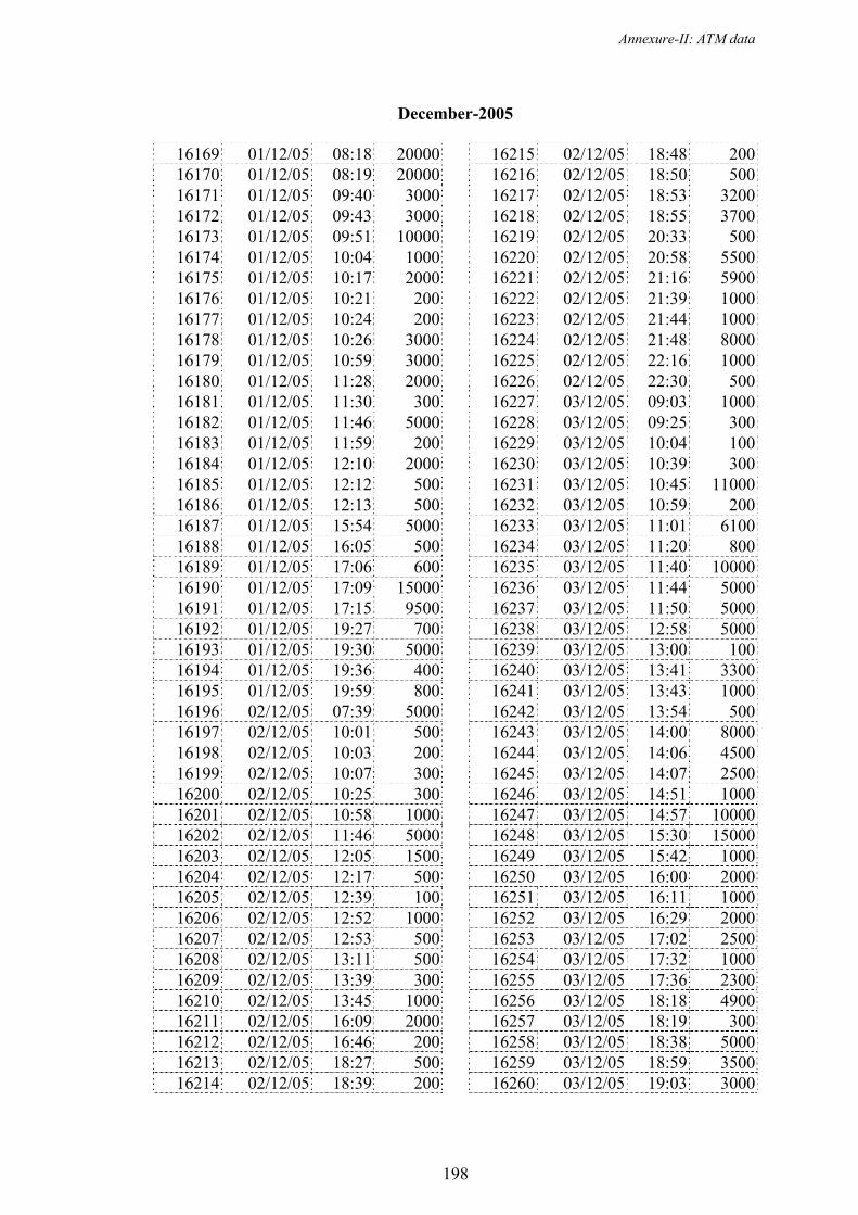
Annexure-II: ATM data
198
December-2005
16169 01/12/05 08:18 2000016170 01/12/05 08:19 2000016171 01/12/05 09:40 300016172 01/12/05 09:43 300016173 01/12/05 09:51 1000016174 01/12/05 10:04 100016175 01/12/05 10:17 200016176 01/12/05 10:21 20016177 01/12/05 10:24 20016178 01/12/05 10:26 300016179 01/12/05 10:59 300016180 01/12/05 11:28 200016181 01/12/05 11:30 30016182 01/12/05 11:46 500016183 01/12/05 11:59 20016184 01/12/05 12:10 200016185 01/12/05 12:12 50016186 01/12/05 12:13 50016187 01/12/05 15:54 500016188 01/12/05 16:05 50016189 01/12/05 17:06 60016190 01/12/05 17:09 1500016191 01/12/05 17:15 950016192 01/12/05 19:27 70016193 01/12/05 19:30 500016194 01/12/05 19:36 40016195 01/12/05 19:59 80016196 02/12/05 07:39 500016197 02/12/05 10:01 50016198 02/12/05 10:03 20016199 02/12/05 10:07 30016200 02/12/05 10:25 30016201 02/12/05 10:58 100016202 02/12/05 11:46 500016203 02/12/05 12:05 150016204 02/12/05 12:17 50016205 02/12/05 12:39 10016206 02/12/05 12:52 100016207 02/12/05 12:53 50016208 02/12/05 13:11 50016209 02/12/05 13:39 30016210 02/12/05 13:45 100016211 02/12/05 16:09 200016212 02/12/05 16:46 20016213 02/12/05 18:27 50016214 02/12/05 18:39 200
16215 02/12/05 18:48 20016216 02/12/05 18:50 50016217 02/12/05 18:53 320016218 02/12/05 18:55 370016219 02/12/05 20:33 50016220 02/12/05 20:58 550016221 02/12/05 21:16 590016222 02/12/05 21:39 100016223 02/12/05 21:44 100016224 02/12/05 21:48 800016225 02/12/05 22:16 100016226 02/12/05 22:30 50016227 03/12/05 09:03 100016228 03/12/05 09:25 30016229 03/12/05 10:04 10016230 03/12/05 10:39 30016231 03/12/05 10:45 1100016232 03/12/05 10:59 20016233 03/12/05 11:01 610016234 03/12/05 11:20 80016235 03/12/05 11:40 1000016236 03/12/05 11:44 500016237 03/12/05 11:50 500016238 03/12/05 12:58 500016239 03/12/05 13:00 10016240 03/12/05 13:41 330016241 03/12/05 13:43 100016242 03/12/05 13:54 50016243 03/12/05 14:00 800016244 03/12/05 14:06 450016245 03/12/05 14:07 250016246 03/12/05 14:51 100016247 03/12/05 14:57 1000016248 03/12/05 15:30 1500016249 03/12/05 15:42 100016250 03/12/05 16:00 200016251 03/12/05 16:11 100016252 03/12/05 16:29 200016253 03/12/05 17:02 250016254 03/12/05 17:32 100016255 03/12/05 17:36 230016256 03/12/05 18:18 490016257 03/12/05 18:19 30016258 03/12/05 18:38 500016259 03/12/05 18:59 350016260 03/12/05 19:03 3000
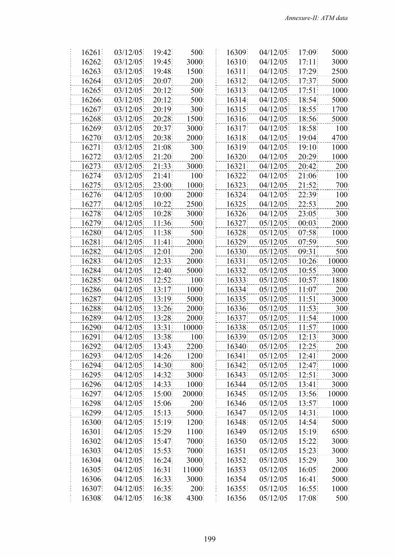
Annexure-II: ATM data
199
16261 03/12/05 19:42 50016262 03/12/05 19:45 300016263 03/12/05 19:48 150016264 03/12/05 20:07 20016265 03/12/05 20:12 50016266 03/12/05 20:12 50016267 03/12/05 20:19 30016268 03/12/05 20:28 150016269 03/12/05 20:37 300016270 03/12/05 20:38 200016271 03/12/05 21:08 30016272 03/12/05 21:20 20016273 03/12/05 21:33 300016274 03/12/05 21:41 10016275 03/12/05 23:00 100016276 04/12/05 10:00 200016277 04/12/05 10:22 250016278 04/12/05 10:28 300016279 04/12/05 11:36 50016280 04/12/05 11:38 50016281 04/12/05 11:41 200016282 04/12/05 12:01 20016283 04/12/05 12:33 200016284 04/12/05 12:40 500016285 04/12/05 12:52 10016286 04/12/05 13:17 100016287 04/12/05 13:19 500016288 04/12/05 13:26 200016289 04/12/05 13:28 200016290 04/12/05 13:31 1000016291 04/12/05 13:38 10016292 04/12/05 13:43 220016293 04/12/05 14:26 120016294 04/12/05 14:30 80016295 04/12/05 14:32 300016296 04/12/05 14:33 100016297 04/12/05 15:00 2000016298 04/12/05 15:06 20016299 04/12/05 15:13 500016300 04/12/05 15:19 120016301 04/12/05 15:29 110016302 04/12/05 15:47 700016303 04/12/05 15:53 700016304 04/12/05 16:24 300016305 04/12/05 16:31 1100016306 04/12/05 16:33 300016307 04/12/05 16:35 20016308 04/12/05 16:38 4300
16309 04/12/05 17:09 500016310 04/12/05 17:11 300016311 04/12/05 17:29 250016312 04/12/05 17:37 500016313 04/12/05 17:51 100016314 04/12/05 18:54 500016315 04/12/05 18:55 170016316 04/12/05 18:56 500016317 04/12/05 18:58 10016318 04/12/05 19:04 470016319 04/12/05 19:10 100016320 04/12/05 20:29 100016321 04/12/05 20:42 20016322 04/12/05 21:06 10016323 04/12/05 21:52 70016324 04/12/05 22:39 10016325 04/12/05 22:53 20016326 04/12/05 23:05 30016327 05/12/05 00:03 200016328 05/12/05 07:58 100016329 05/12/05 07:59 50016330 05/12/05 09:31 50016331 05/12/05 10:26 1000016332 05/12/05 10:55 300016333 05/12/05 10:57 180016334 05/12/05 11:07 20016335 05/12/05 11:51 300016336 05/12/05 11:53 30016337 05/12/05 11:54 100016338 05/12/05 11:57 100016339 05/12/05 12:13 300016340 05/12/05 12:25 20016341 05/12/05 12:41 200016342 05/12/05 12:47 100016343 05/12/05 12:51 300016344 05/12/05 13:41 300016345 05/12/05 13:56 1000016346 05/12/05 13:57 100016347 05/12/05 14:31 100016348 05/12/05 14:54 500016349 05/12/05 15:19 650016350 05/12/05 15:22 300016351 05/12/05 15:23 300016352 05/12/05 15:29 30016353 05/12/05 16:05 200016354 05/12/05 16:41 500016355 05/12/05 16:55 100016356 05/12/05 17:08 500
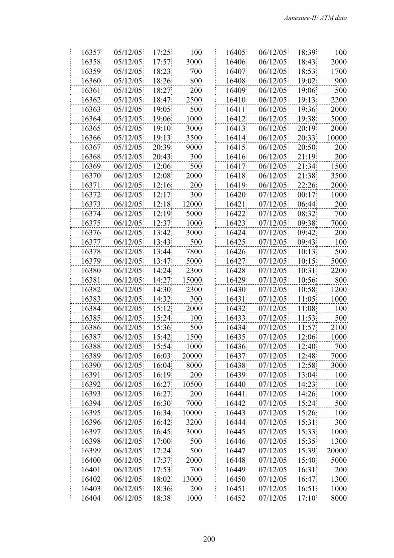
Annexure-II: ATM data
200
16357 05/12/05 17:25 10016358 05/12/05 17:57 300016359 05/12/05 18:23 70016360 05/12/05 18:26 80016361 05/12/05 18:27 20016362 05/12/05 18:47 250016363 05/12/05 19:05 50016364 05/12/05 19:06 100016365 05/12/05 19:10 300016366 05/12/05 19:13 350016367 05/12/05 20:39 900016368 05/12/05 20:43 30016369 06/12/05 12:06 50016370 06/12/05 12:08 200016371 06/12/05 12:16 20016372 06/12/05 12:17 30016373 06/12/05 12:18 1200016374 06/12/05 12:19 500016375 06/12/05 12:37 100016376 06/12/05 13:42 300016377 06/12/05 13:43 50016378 06/12/05 13:44 780016379 06/12/05 13:47 500016380 06/12/05 14:24 230016381 06/12/05 14:27 1500016382 06/12/05 14:30 230016383 06/12/05 14:32 30016384 06/12/05 15:12 200016385 06/12/05 15:24 10016386 06/12/05 15:36 50016387 06/12/05 15:42 150016388 06/12/05 15:54 100016389 06/12/05 16:03 2000016390 06/12/05 16:04 800016391 06/12/05 16:19 20016392 06/12/05 16:27 1050016393 06/12/05 16:27 20016394 06/12/05 16:30 700016395 06/12/05 16:34 1000016396 06/12/05 16:42 320016397 06/12/05 16:45 300016398 06/12/05 17:00 50016399 06/12/05 17:24 50016400 06/12/05 17:37 200016401 06/12/05 17:53 70016402 06/12/05 18:02 1300016403 06/12/05 18:36 20016404 06/12/05 18:38 1000
16405 06/12/05 18:39 10016406 06/12/05 18:43 200016407 06/12/05 18:53 170016408 06/12/05 19:02 90016409 06/12/05 19:06 50016410 06/12/05 19:13 220016411 06/12/05 19:36 200016412 06/12/05 19:38 500016413 06/12/05 20:19 200016414 06/12/05 20:33 1000016415 06/12/05 20:50 20016416 06/12/05 21:19 20016417 06/12/05 21:34 150016418 06/12/05 21:38 350016419 06/12/05 22:26 200016420 07/12/05 00:17 100016421 07/12/05 06:44 20016422 07/12/05 08:32 70016423 07/12/05 09:38 700016424 07/12/05 09:42 20016425 07/12/05 09:43 10016426 07/12/05 10:13 50016427 07/12/05 10:15 500016428 07/12/05 10:31 220016429 07/12/05 10:56 80016430 07/12/05 10:58 120016431 07/12/05 11:05 100016432 07/12/05 11:08 10016433 07/12/05 11:53 50016434 07/12/05 11:57 210016435 07/12/05 12:06 100016436 07/12/05 12:40 70016437 07/12/05 12:48 700016438 07/12/05 12:58 300016439 07/12/05 13:04 10016440 07/12/05 14:23 10016441 07/12/05 14:26 100016442 07/12/05 15:24 50016443 07/12/05 15:26 10016444 07/12/05 15:31 30016445 07/12/05 15:33 100016446 07/12/05 15:35 130016447 07/12/05 15:39 2000016448 07/12/05 15:40 500016449 07/12/05 16:31 20016450 07/12/05 16:47 130016451 07/12/05 16:51 100016452 07/12/05 17:10 8000

Annexure-II: ATM data
201
16453 07/12/05 17:12 900016454 07/12/05 17:21 300016455 07/12/05 17:40 200016456 07/12/05 17:51 120016457 07/12/05 17:54 20016458 07/12/05 17:55 300016459 07/12/05 17:56 300016460 07/12/05 18:10 200016461 07/12/05 18:10 100016462 07/12/05 18:11 100016463 07/12/05 18:14 10016464 07/12/05 18:21 70016465 07/12/05 18:30 1000016466 07/12/05 18:31 250016467 07/12/05 18:39 500016468 07/12/05 18:55 200016469 07/12/05 19:23 300016470 07/12/05 20:33 10016471 07/12/05 20:34 100016472 07/12/05 20:50 200016473 07/12/05 21:36 20016474 07/12/05 21:39 10016475 07/12/05 22:08 10016476 07/12/05 22:27 200016477 07/12/05 22:27 300016478 07/12/05 23:05 20016479 07/12/05 23:56 50016480 08/12/05 08:32 200016481 08/12/05 09:19 310016482 08/12/05 09:21 220016483 08/12/05 10:07 120016484 08/12/05 10:09 200016485 08/12/05 10:35 150016486 08/12/05 10:42 120016487 08/12/05 10:45 110016488 08/12/05 10:55 50016489 08/12/05 11:12 20016490 08/12/05 11:18 250016491 08/12/05 11:28 150016492 08/12/05 11:29 10016493 08/12/05 11:50 550016494 08/12/05 11:57 130016495 08/12/05 12:44 1000016496 08/12/05 12:57 50016497 08/12/05 13:32 50016498 08/12/05 13:47 20016499 08/12/05 13:51 1000016500 08/12/05 13:59 100
16501 08/12/05 14:16 680016502 08/12/05 16:01 220016503 08/12/05 16:03 230016504 08/12/05 16:05 10016505 08/12/05 16:06 100016506 08/12/05 16:08 50016507 08/12/05 16:24 800016508 08/12/05 17:00 90016509 08/12/05 17:17 20016510 08/12/05 17:22 100016511 08/12/05 17:57 30016512 08/12/05 18:03 200016513 08/12/05 18:17 100016514 08/12/05 18:18 100016515 08/12/05 18:26 10016516 08/12/05 19:22 200016517 08/12/05 19:33 1000016518 08/12/05 20:00 350016519 08/12/05 20:09 100016520 08/12/05 20:10 100016521 08/12/05 20:21 2000016522 08/12/05 20:44 700016523 08/12/05 23:14 800016524 09/12/05 00:07 150016525 09/12/05 00:23 10016526 09/12/05 09:21 70016527 09/12/05 09:34 300016528 09/12/05 09:35 200016529 09/12/05 10:00 200016530 09/12/05 10:35 10016531 09/12/05 10:44 20016532 09/12/05 11:29 50016533 09/12/05 11:33 800016534 09/12/05 11:36 1000016535 09/12/05 11:39 800016536 09/12/05 11:47 120016537 09/12/05 11:49 50016538 09/12/05 12:09 200016539 09/12/05 12:10 2000016540 09/12/05 12:29 100016541 09/12/05 12:43 300016542 09/12/05 12:44 300016543 09/12/05 13:03 30016544 09/12/05 13:26 50016545 09/12/05 13:43 50016546 09/12/05 13:52 1650016547 09/12/05 14:16 200016548 09/12/05 14:24 500

Annexure-II: ATM data
202
16549 09/12/05 14:49 150016550 09/12/05 15:14 100016551 09/12/05 16:42 30016552 09/12/05 17:32 150016553 09/12/05 18:00 50016554 09/12/05 18:00 50016555 09/12/05 18:01 10016556 09/12/05 18:30 500016557 09/12/05 18:42 10016558 09/12/05 18:50 20016559 09/12/05 19:25 150016560 09/12/05 19:30 10016561 09/12/05 19:33 20016562 09/12/05 19:43 10016563 09/12/05 20:01 80016564 09/12/05 20:04 10016565 09/12/05 20:07 50016566 09/12/05 20:19 300016567 09/12/05 20:30 20016568 09/12/05 20:32 100016569 09/12/05 22:28 200016570 10/12/05 07:44 200016571 10/12/05 07:45 50016572 10/12/05 07:46 50016573 10/12/05 09:48 200016574 10/12/05 10:01 50016575 10/12/05 10:02 1500016576 10/12/05 10:06 100016577 10/12/05 10:08 100016578 10/12/05 10:37 200016579 10/12/05 11:01 30016580 10/12/05 11:03 500016581 10/12/05 11:08 100016582 10/12/05 11:18 200016583 10/12/05 11:19 30016584 10/12/05 11:28 100016585 10/12/05 11:34 370016586 10/12/05 11:38 800016587 10/12/05 11:43 20016588 10/12/05 11:47 920016589 10/12/05 11:54 200016590 10/12/05 11:55 20016591 10/12/05 11:56 50016592 10/12/05 12:13 100016593 10/12/05 12:25 30016594 10/12/05 12:27 50016595 10/12/05 12:33 100016596 10/12/05 12:38 3000
16597 10/12/05 13:06 110016598 10/12/05 13:27 230016599 10/12/05 13:37 30016600 10/12/05 13:42 10016601 10/12/05 13:51 70016602 10/12/05 13:59 200016603 10/12/05 14:13 1700016604 10/12/05 14:41 100016605 10/12/05 14:59 200016606 10/12/05 15:33 800016607 10/12/05 15:34 800016608 10/12/05 15:52 1500016609 10/12/05 15:58 30016610 10/12/05 16:24 100016611 10/12/05 16:35 1200016612 10/12/05 16:41 500016613 10/12/05 16:55 200016614 10/12/05 16:58 200016615 10/12/05 17:26 50016616 10/12/05 17:50 20016617 10/12/05 17:51 50016618 10/12/05 17:57 10016619 10/12/05 18:06 110016620 10/12/05 18:07 20016621 10/12/05 18:08 10016622 10/12/05 18:10 300016623 10/12/05 18:10 200016624 10/12/05 18:13 100016625 10/12/05 18:25 20016626 10/12/05 18:34 50016627 10/12/05 18:38 20016628 10/12/05 18:47 50016629 10/12/05 18:56 130016630 10/12/05 19:05 180016631 10/12/05 19:15 50016632 10/12/05 19:35 100016633 10/12/05 19:37 300016634 10/12/05 19:45 30016635 10/12/05 20:33 80016636 10/12/05 20:50 10016637 10/12/05 21:14 10016638 10/12/05 21:23 310016639 10/12/05 21:29 200016640 10/12/05 21:31 50016641 10/12/05 21:40 90016642 10/12/05 22:08 20016643 11/12/05 00:25 30016644 11/12/05 01:14 100

Annexure-II: ATM data
203
16645 11/12/05 09:42 2000016646 11/12/05 09:43 800016647 11/12/05 10:30 100016648 11/12/05 10:50 300016649 11/12/05 11:11 30016650 11/12/05 11:24 200016651 11/12/05 11:51 150016652 11/12/05 11:58 200016653 11/12/05 12:06 110016654 11/12/05 12:11 1020016655 11/12/05 12:31 2000016656 11/12/05 12:33 1500016657 11/12/05 12:46 200016658 11/12/05 13:14 200016659 11/12/05 13:22 150016660 11/12/05 13:26 200016661 11/12/05 14:18 120016662 11/12/05 15:09 200016663 11/12/05 15:39 50016664 11/12/05 15:41 10016665 11/12/05 16:40 50016666 11/12/05 16:54 500016667 11/12/05 17:04 50016668 11/12/05 17:05 50016669 11/12/05 17:15 50016670 11/12/05 17:28 20016671 11/12/05 17:40 1000016672 11/12/05 17:47 100016673 11/12/05 17:52 50016674 11/12/05 18:10 500016675 11/12/05 18:14 30016676 11/12/05 18:23 100016677 11/12/05 18:24 100016678 11/12/05 18:25 100016679 11/12/05 18:35 100016680 11/12/05 18:38 20016681 11/12/05 18:59 350016682 11/12/05 19:07 50016683 11/12/05 19:22 250016684 11/12/05 19:27 2000016685 11/12/05 19:38 100016686 11/12/05 19:43 10016687 11/12/05 19:55 90016688 11/12/05 20:10 50016689 11/12/05 20:16 100016690 11/12/05 21:24 300016691 11/12/05 22:13 500016692 11/12/05 22:27 500
16693 11/12/05 22:32 300016694 11/12/05 23:06 20016695 11/12/05 23:07 150016696 11/12/05 23:29 30016697 11/12/05 23:35 30016698 11/12/05 23:45 100016699 12/12/05 08:58 1700016700 12/12/05 09:49 50016701 12/12/05 11:04 1000016702 12/12/05 11:37 120016703 12/12/05 11:58 100016704 12/12/05 12:16 200016705 12/12/05 12:29 50016706 12/12/05 12:32 300016707 12/12/05 12:45 450016708 12/12/05 12:47 500016709 12/12/05 13:04 1000016710 12/12/05 13:34 2200016711 12/12/05 13:40 10016712 12/12/05 14:21 300016713 12/12/05 15:00 50016714 12/12/05 15:07 100016715 12/12/05 16:01 100016716 12/12/05 16:14 120016717 12/12/05 16:50 900016718 12/12/05 17:06 300016719 12/12/05 17:08 20016720 12/12/05 17:21 50016721 12/12/05 18:10 10016722 12/12/05 18:19 1300016723 12/12/05 18:59 300016724 12/12/05 19:17 20016725 12/12/05 19:24 30016726 12/12/05 19:37 200016727 12/12/05 20:30 300016728 12/12/05 20:55 1500016729 12/12/05 21:06 50016730 12/12/05 21:20 20016731 12/12/05 23:49 10016732 12/12/05 23:51 10016733 12/12/05 23:52 10016734 13/12/05 01:31 10016735 13/12/05 09:11 20016736 13/12/05 09:35 300016737 13/12/05 09:36 300016738 13/12/05 10:35 100016739 13/12/05 10:36 100016740 13/12/05 10:48 500
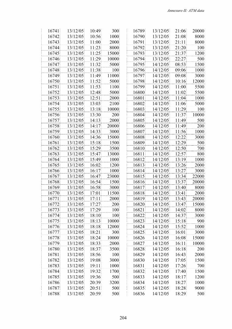
Annexure-II: ATM data
204
16741 13/12/05 10:49 30016742 13/12/05 10:56 100016743 13/12/05 11:00 200016744 13/12/05 11:23 800016745 13/12/05 11:25 1500016746 13/12/05 11:29 1000016747 13/12/05 11:32 500016748 13/12/05 11:38 10016749 13/12/05 11:49 1100016750 13/12/05 11:52 500016751 13/12/05 11:53 110016752 13/12/05 12:48 500016753 13/12/05 12:51 200016754 13/12/05 13:03 210016755 13/12/05 13:18 1000016756 13/12/05 13:30 20016757 13/12/05 14:13 200016758 13/12/05 14:17 2000016759 13/12/05 14:33 300016760 13/12/05 14:36 1500016761 13/12/05 15:18 150016762 13/12/05 15:29 350016763 13/12/05 15:47 1300016764 13/12/05 15:49 100016765 13/12/05 16:02 120016766 13/12/05 16:17 100016767 13/12/05 16:47 2300016768 13/12/05 16:54 150016769 13/12/05 16:58 300016770 13/12/05 17:01 1150016771 13/12/05 17:11 200016772 13/12/05 17:27 20016773 13/12/05 17:29 10016774 13/12/05 18:10 10016775 13/12/05 18:13 1000016776 13/12/05 18:18 1200016777 13/12/05 18:21 30016778 13/12/05 18:24 1000016779 13/12/05 18:33 200016780 13/12/05 18:37 350016781 13/12/05 18:56 10016782 13/12/05 19:08 300016783 13/12/05 19:11 100016784 13/12/05 19:32 170016785 13/12/05 19:36 50016786 13/12/05 20:39 320016787 13/12/05 20:51 50016788 13/12/05 20:59 500
16789 13/12/05 21:06 2000016790 13/12/05 21:08 800016791 13/12/05 21:11 800016792 13/12/05 21:20 10016793 13/12/05 21:37 120016794 13/12/05 22:27 50016795 14/12/05 08:53 150016796 14/12/05 09:06 100016797 14/12/05 09:08 300016798 14/12/05 10:16 1200016799 14/12/05 11:00 550016800 14/12/05 11:02 550016801 14/12/05 11:04 100016802 14/12/05 11:06 500016803 14/12/05 11:29 10016804 14/12/05 11:37 1000016805 14/12/05 11:49 50016806 14/12/05 11:49 20016807 14/12/05 11:56 100016808 14/12/05 12:22 300016809 14/12/05 12:29 50016810 14/12/05 12:50 70016811 14/12/05 12:57 80016812 14/12/05 13:19 100016813 14/12/05 13:26 200016814 14/12/05 13:27 300016815 14/12/05 13:34 2200016816 14/12/05 13:37 2000016817 14/12/05 13:40 800016818 14/12/05 13:41 200016819 14/12/05 13:43 2000016820 14/12/05 13:47 1500016821 14/12/05 14:02 800016822 14/12/05 14:37 300016823 14/12/05 15:18 90016824 14/12/05 15:52 100016825 14/12/05 16:01 300016826 14/12/05 16:08 1500016827 14/12/05 16:11 1000016828 14/12/05 16:18 20016829 14/12/05 16:43 200016830 14/12/05 17:05 150016831 14/12/05 17:26 70016832 14/12/05 17:40 150016833 14/12/05 18:17 120016834 14/12/05 18:27 100016835 14/12/05 18:28 900016836 14/12/05 18:29 500

Annexure-II: ATM data
205
16837 14/12/05 18:33 30016838 14/12/05 19:04 2000016839 14/12/05 19:06 800016840 14/12/05 19:08 100016841 14/12/05 19:34 30016842 14/12/05 19:56 20016843 14/12/05 20:46 500016844 15/12/05 07:42 30016845 15/12/05 09:41 50016846 15/12/05 09:48 2000016847 15/12/05 09:49 500016848 15/12/05 09:51 50016849 15/12/05 10:14 20016850 15/12/05 10:26 10016851 15/12/05 10:40 10016852 15/12/05 10:41 100016853 15/12/05 10:47 70016854 15/12/05 10:48 50016855 15/12/05 10:55 1970016856 15/12/05 10:57 20016857 15/12/05 11:10 300016858 15/12/05 11:12 50016859 15/12/05 11:45 20016860 15/12/05 12:00 450016861 15/12/05 12:11 50016862 15/12/05 12:20 2000016863 15/12/05 12:22 800016864 15/12/05 12:51 100016865 15/12/05 12:53 500016866 15/12/05 13:16 70016867 15/12/05 13:20 30016868 15/12/05 13:21 50016869 15/12/05 14:04 2000016870 15/12/05 14:06 1200016871 15/12/05 14:26 320016872 15/12/05 14:27 800016873 15/12/05 14:28 200016874 15/12/05 16:01 100016875 15/12/05 16:20 700016876 15/12/05 16:35 500016877 15/12/05 16:58 500016878 15/12/05 16:59 500016879 15/12/05 17:56 20016880 15/12/05 18:00 500016881 15/12/05 18:10 200016882 15/12/05 18:12 250016883 15/12/05 18:24 1000016884 15/12/05 18:53 800
16885 15/12/05 19:00 2100016886 15/12/05 19:01 100016887 15/12/05 19:11 10016888 15/12/05 19:12 100016889 15/12/05 19:14 10016890 15/12/05 19:21 50016891 15/12/05 19:24 50016892 15/12/05 21:11 20016893 15/12/05 21:27 1650016894 15/12/05 21:32 50016895 15/12/05 22:38 300016896 15/12/05 22:43 100016897 16/12/05 00:32 2000016898 16/12/05 06:13 50016899 16/12/05 06:13 500016900 16/12/05 09:24 250016901 16/12/05 09:41 100016902 16/12/05 09:50 20016903 16/12/05 09:52 2000016904 16/12/05 09:52 800016905 16/12/05 09:54 200016906 16/12/05 11:06 500016907 16/12/05 11:28 100016908 16/12/05 12:00 10016909 16/12/05 12:28 100016910 16/12/05 12:36 30016911 16/12/05 12:55 700016912 16/12/05 13:08 50016913 16/12/05 13:09 300016914 16/12/05 14:40 30016915 16/12/05 17:11 1200016916 16/12/05 17:16 20016917 16/12/05 17:22 100016918 16/12/05 18:10 2000016919 16/12/05 19:19 300016920 16/12/05 19:27 200016921 16/12/05 19:43 100016922 16/12/05 20:29 20016923 16/12/05 22:56 20016924 17/12/05 09:39 200016925 17/12/05 09:53 50016926 17/12/05 10:00 500016927 17/12/05 10:02 50016928 17/12/05 10:03 300016929 17/12/05 10:10 1000016930 17/12/05 10:29 330016931 17/12/05 10:33 20016932 17/12/05 10:39 1800
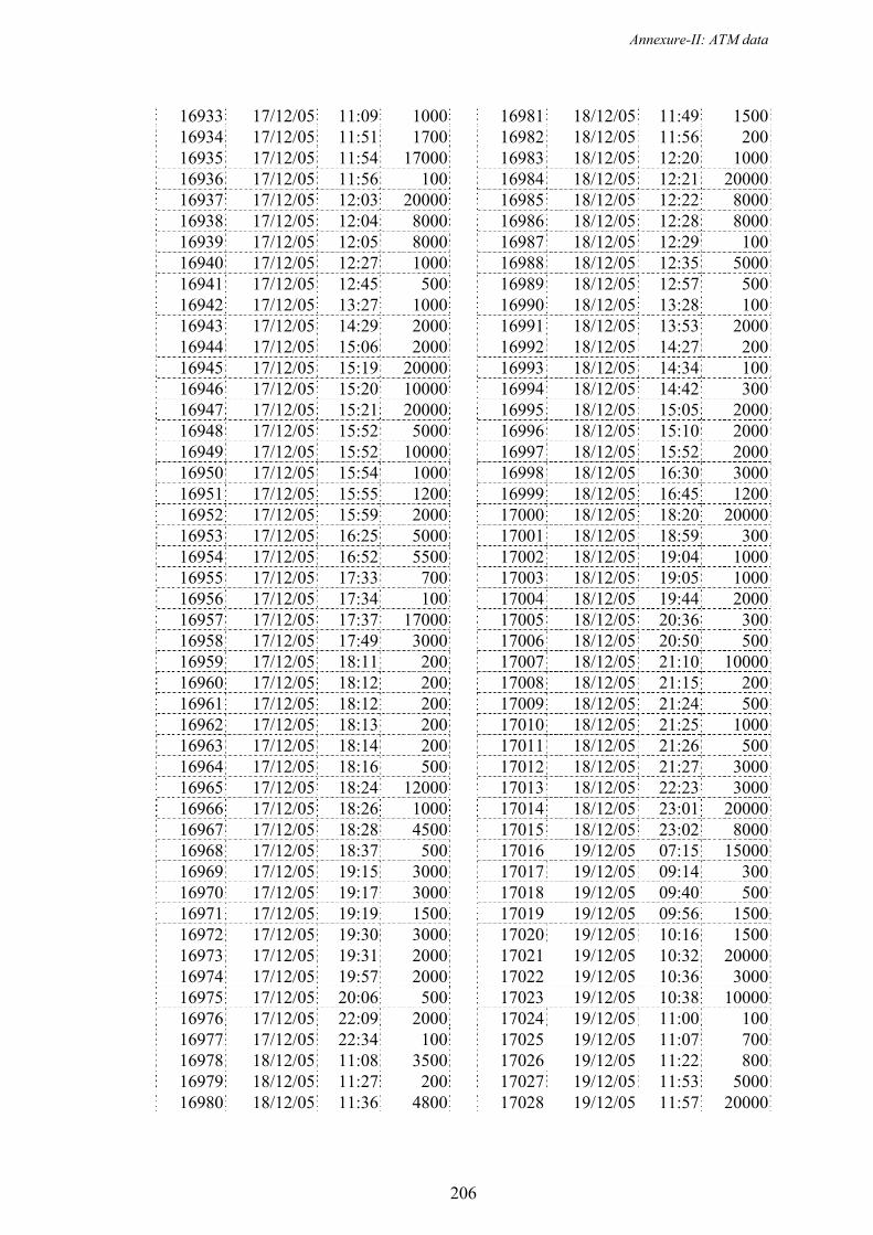
Annexure-II: ATM data
206
16933 17/12/05 11:09 100016934 17/12/05 11:51 170016935 17/12/05 11:54 1700016936 17/12/05 11:56 10016937 17/12/05 12:03 2000016938 17/12/05 12:04 800016939 17/12/05 12:05 800016940 17/12/05 12:27 100016941 17/12/05 12:45 50016942 17/12/05 13:27 100016943 17/12/05 14:29 200016944 17/12/05 15:06 200016945 17/12/05 15:19 2000016946 17/12/05 15:20 1000016947 17/12/05 15:21 2000016948 17/12/05 15:52 500016949 17/12/05 15:52 1000016950 17/12/05 15:54 100016951 17/12/05 15:55 120016952 17/12/05 15:59 200016953 17/12/05 16:25 500016954 17/12/05 16:52 550016955 17/12/05 17:33 70016956 17/12/05 17:34 10016957 17/12/05 17:37 1700016958 17/12/05 17:49 300016959 17/12/05 18:11 20016960 17/12/05 18:12 20016961 17/12/05 18:12 20016962 17/12/05 18:13 20016963 17/12/05 18:14 20016964 17/12/05 18:16 50016965 17/12/05 18:24 1200016966 17/12/05 18:26 100016967 17/12/05 18:28 450016968 17/12/05 18:37 50016969 17/12/05 19:15 300016970 17/12/05 19:17 300016971 17/12/05 19:19 150016972 17/12/05 19:30 300016973 17/12/05 19:31 200016974 17/12/05 19:57 200016975 17/12/05 20:06 50016976 17/12/05 22:09 200016977 17/12/05 22:34 10016978 18/12/05 11:08 350016979 18/12/05 11:27 20016980 18/12/05 11:36 4800
16981 18/12/05 11:49 150016982 18/12/05 11:56 20016983 18/12/05 12:20 100016984 18/12/05 12:21 2000016985 18/12/05 12:22 800016986 18/12/05 12:28 800016987 18/12/05 12:29 10016988 18/12/05 12:35 500016989 18/12/05 12:57 50016990 18/12/05 13:28 10016991 18/12/05 13:53 200016992 18/12/05 14:27 20016993 18/12/05 14:34 10016994 18/12/05 14:42 30016995 18/12/05 15:05 200016996 18/12/05 15:10 200016997 18/12/05 15:52 200016998 18/12/05 16:30 300016999 18/12/05 16:45 120017000 18/12/05 18:20 2000017001 18/12/05 18:59 30017002 18/12/05 19:04 100017003 18/12/05 19:05 100017004 18/12/05 19:44 200017005 18/12/05 20:36 30017006 18/12/05 20:50 50017007 18/12/05 21:10 1000017008 18/12/05 21:15 20017009 18/12/05 21:24 50017010 18/12/05 21:25 100017011 18/12/05 21:26 50017012 18/12/05 21:27 300017013 18/12/05 22:23 300017014 18/12/05 23:01 2000017015 18/12/05 23:02 800017016 19/12/05 07:15 1500017017 19/12/05 09:14 30017018 19/12/05 09:40 50017019 19/12/05 09:56 150017020 19/12/05 10:16 150017021 19/12/05 10:32 2000017022 19/12/05 10:36 300017023 19/12/05 10:38 1000017024 19/12/05 11:00 10017025 19/12/05 11:07 70017026 19/12/05 11:22 80017027 19/12/05 11:53 500017028 19/12/05 11:57 20000

Annexure-II: ATM data
207
17029 19/12/05 11:58 800017030 19/12/05 12:15 120017031 19/12/05 12:17 100017032 19/12/05 12:19 350017033 19/12/05 12:27 1000017034 19/12/05 12:28 120017035 19/12/05 12:30 10017036 19/12/05 12:32 100017037 19/12/05 12:57 50017038 19/12/05 13:23 50017039 19/12/05 13:28 50017040 19/12/05 14:46 2000017041 19/12/05 14:47 1200017042 19/12/05 14:50 200017043 19/12/05 14:52 300017044 19/12/05 16:29 10017045 19/12/05 16:33 330017046 19/12/05 16:49 300017047 19/12/05 17:08 200017048 19/12/05 17:15 50017049 19/12/05 17:16 20017050 19/12/05 17:38 430017051 19/12/05 17:42 50017052 19/12/05 17:43 100017053 19/12/05 18:12 20017054 19/12/05 18:17 2000017055 19/12/05 18:26 300017056 19/12/05 18:30 50017057 19/12/05 18:37 200017058 19/12/05 18:39 50017059 19/12/05 19:01 300017060 19/12/05 19:02 300017061 19/12/05 19:03 50017062 19/12/05 19:09 690017063 19/12/05 19:17 500017064 19/12/05 19:24 20017065 19/12/05 19:46 250017066 19/12/05 19:57 150017067 19/12/05 20:04 100017068 19/12/05 20:16 200017069 19/12/05 21:47 100017070 19/12/05 21:53 200017071 19/12/05 21:56 50017072 19/12/05 23:20 100017073 19/12/05 23:34 10017074 20/12/05 08:42 800017075 20/12/05 08:49 10017076 20/12/05 08:50 8000
17077 20/12/05 10:20 2000017078 20/12/05 11:08 100017079 20/12/05 11:09 200017080 20/12/05 11:28 70017081 20/12/05 11:36 300017082 20/12/05 12:21 350017083 20/12/05 12:23 50017084 20/12/05 12:24 100017085 20/12/05 12:36 120017086 20/12/05 13:23 50017087 20/12/05 13:31 1000017088 20/12/05 13:41 200017089 20/12/05 14:15 500017090 20/12/05 14:18 300017091 20/12/05 14:38 800017092 20/12/05 14:39 2000017093 20/12/05 14:50 20017094 20/12/05 15:18 250017095 20/12/05 16:31 150017096 20/12/05 17:01 10017097 20/12/05 17:19 700017098 20/12/05 18:06 150017099 20/12/05 18:07 20017100 20/12/05 18:09 800017101 20/12/05 18:29 610017102 20/12/05 18:31 750017103 20/12/05 19:45 30017104 20/12/05 19:49 20017105 20/12/05 20:11 2000017106 20/12/05 20:12 700017107 20/12/05 20:13 100017108 20/12/05 20:14 30017109 20/12/05 20:15 100017110 20/12/05 20:43 100017111 20/12/05 20:49 50017112 20/12/05 20:50 50017113 20/12/05 20:51 100017114 20/12/05 20:53 20017115 20/12/05 21:33 10017116 20/12/05 21:34 30017117 20/12/05 21:43 100017118 20/12/05 21:45 10017119 20/12/05 22:16 30017120 20/12/05 22:22 510017121 21/12/05 09:16 200017122 21/12/05 09:17 50017123 21/12/05 09:47 20017124 21/12/05 11:13 300
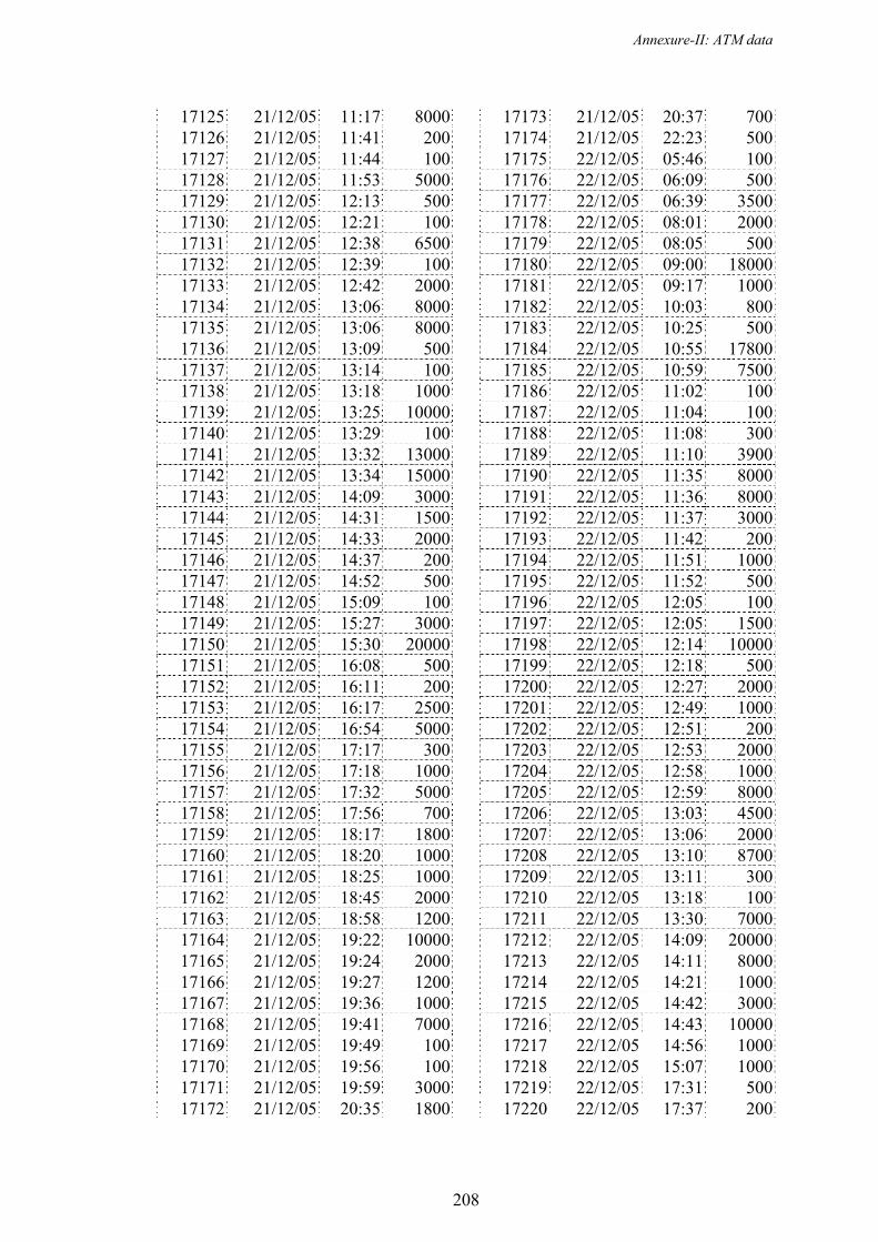
Annexure-II: ATM data
208
17125 21/12/05 11:17 800017126 21/12/05 11:41 20017127 21/12/05 11:44 10017128 21/12/05 11:53 500017129 21/12/05 12:13 50017130 21/12/05 12:21 10017131 21/12/05 12:38 650017132 21/12/05 12:39 10017133 21/12/05 12:42 200017134 21/12/05 13:06 800017135 21/12/05 13:06 800017136 21/12/05 13:09 50017137 21/12/05 13:14 10017138 21/12/05 13:18 100017139 21/12/05 13:25 1000017140 21/12/05 13:29 10017141 21/12/05 13:32 1300017142 21/12/05 13:34 1500017143 21/12/05 14:09 300017144 21/12/05 14:31 150017145 21/12/05 14:33 200017146 21/12/05 14:37 20017147 21/12/05 14:52 50017148 21/12/05 15:09 10017149 21/12/05 15:27 300017150 21/12/05 15:30 2000017151 21/12/05 16:08 50017152 21/12/05 16:11 20017153 21/12/05 16:17 250017154 21/12/05 16:54 500017155 21/12/05 17:17 30017156 21/12/05 17:18 100017157 21/12/05 17:32 500017158 21/12/05 17:56 70017159 21/12/05 18:17 180017160 21/12/05 18:20 100017161 21/12/05 18:25 100017162 21/12/05 18:45 200017163 21/12/05 18:58 120017164 21/12/05 19:22 1000017165 21/12/05 19:24 200017166 21/12/05 19:27 120017167 21/12/05 19:36 100017168 21/12/05 19:41 700017169 21/12/05 19:49 10017170 21/12/05 19:56 10017171 21/12/05 19:59 300017172 21/12/05 20:35 1800
17173 21/12/05 20:37 70017174 21/12/05 22:23 50017175 22/12/05 05:46 10017176 22/12/05 06:09 50017177 22/12/05 06:39 350017178 22/12/05 08:01 200017179 22/12/05 08:05 50017180 22/12/05 09:00 1800017181 22/12/05 09:17 100017182 22/12/05 10:03 80017183 22/12/05 10:25 50017184 22/12/05 10:55 1780017185 22/12/05 10:59 750017186 22/12/05 11:02 10017187 22/12/05 11:04 10017188 22/12/05 11:08 30017189 22/12/05 11:10 390017190 22/12/05 11:35 800017191 22/12/05 11:36 800017192 22/12/05 11:37 300017193 22/12/05 11:42 20017194 22/12/05 11:51 100017195 22/12/05 11:52 50017196 22/12/05 12:05 10017197 22/12/05 12:05 150017198 22/12/05 12:14 1000017199 22/12/05 12:18 50017200 22/12/05 12:27 200017201 22/12/05 12:49 100017202 22/12/05 12:51 20017203 22/12/05 12:53 200017204 22/12/05 12:58 100017205 22/12/05 12:59 800017206 22/12/05 13:03 450017207 22/12/05 13:06 200017208 22/12/05 13:10 870017209 22/12/05 13:11 30017210 22/12/05 13:18 10017211 22/12/05 13:30 700017212 22/12/05 14:09 2000017213 22/12/05 14:11 800017214 22/12/05 14:21 100017215 22/12/05 14:42 300017216 22/12/05 14:43 1000017217 22/12/05 14:56 100017218 22/12/05 15:07 100017219 22/12/05 17:31 50017220 22/12/05 17:37 200

Annexure-II: ATM data
209
17221 22/12/05 17:50 1000017222 22/12/05 18:04 200017223 22/12/05 18:05 20017224 22/12/05 18:29 100017225 22/12/05 19:03 100017226 22/12/05 19:15 200017227 22/12/05 19:50 530017228 22/12/05 19:52 50017229 22/12/05 19:54 200017230 22/12/05 20:04 30017231 22/12/05 21:19 10017232 22/12/05 22:11 100017233 22/12/05 22:23 50017234 23/12/05 07:52 100017235 23/12/05 08:01 50017236 23/12/05 08:49 50017237 23/12/05 08:57 150017238 23/12/05 09:30 50017239 23/12/05 09:36 300017240 23/12/05 09:56 50017241 23/12/05 10:11 100017242 23/12/05 10:20 300017243 23/12/05 10:23 200017244 23/12/05 10:28 200017245 23/12/05 10:33 500017246 23/12/05 11:23 200017247 23/12/05 11:41 50017248 23/12/05 11:48 90017249 23/12/05 11:58 100017250 23/12/05 12:00 90017251 23/12/05 12:19 50017252 23/12/05 12:28 30017253 23/12/05 12:30 100017254 23/12/05 12:46 200017255 23/12/05 12:58 20017256 23/12/05 13:38 500017257 23/12/05 13:44 10017258 23/12/05 13:59 250017259 23/12/05 15:07 2000017260 23/12/05 16:02 1000017261 23/12/05 17:05 300017262 23/12/05 18:21 50017263 23/12/05 18:29 50017264 23/12/05 18:40 500017265 23/12/05 18:44 150017266 23/12/05 18:47 10017267 23/12/05 19:51 500017268 23/12/05 20:07 2000
17269 23/12/05 20:28 100017270 23/12/05 21:06 10017271 23/12/05 21:16 10017272 23/12/05 21:40 1000017273 23/12/05 22:01 50017274 24/12/05 09:13 10017275 24/12/05 09:52 30017276 24/12/05 10:12 1500017277 24/12/05 10:18 10017278 24/12/05 10:19 250017279 24/12/05 10:21 200017280 24/12/05 10:22 210017281 24/12/05 10:25 20017282 24/12/05 10:27 550017283 24/12/05 10:40 50017284 24/12/05 10:53 10017285 24/12/05 10:55 50017286 24/12/05 11:17 100017287 24/12/05 11:27 250017288 24/12/05 11:31 10017289 24/12/05 11:35 300017290 24/12/05 11:41 1500017291 24/12/05 11:43 200017292 24/12/05 11:53 100017293 24/12/05 12:09 200017294 24/12/05 12:26 50017295 24/12/05 12:28 2000017296 24/12/05 12:38 50017297 24/12/05 12:39 150017298 24/12/05 12:54 30017299 24/12/05 13:00 50017300 24/12/05 13:25 50017301 24/12/05 13:33 1000017302 24/12/05 13:47 500017303 24/12/05 13:52 70017304 24/12/05 13:57 100017305 24/12/05 13:58 50017306 24/12/05 13:58 50017307 24/12/05 14:09 100017308 24/12/05 14:22 800017309 24/12/05 14:33 2000017310 24/12/05 14:44 100017311 24/12/05 14:45 500017312 24/12/05 14:54 200017313 24/12/05 15:10 1000017314 24/12/05 15:12 200017315 24/12/05 15:19 200017316 24/12/05 15:20 5000
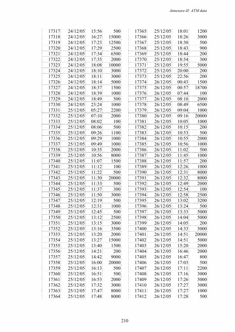
Annexure-II: ATM data
210
17317 24/12/05 15:56 50017318 24/12/05 16:27 1500017319 24/12/05 17:23 1250017320 24/12/05 17:29 250017321 24/12/05 17:34 650017322 24/12/05 17:35 200017323 24/12/05 18:08 1000017324 24/12/05 18:10 300017325 24/12/05 18:11 300017326 24/12/05 18:14 500017327 24/12/05 18:37 150017328 24/12/05 18:39 100017329 24/12/05 18:49 50017330 24/12/05 23:24 100017331 25/12/05 05:27 220017332 25/12/05 07:10 200017333 25/12/05 08:02 10017334 25/12/05 08:06 50017335 25/12/05 09:26 110017336 25/12/05 09:29 100017337 25/12/05 09:49 100017338 25/12/05 10:35 200017339 25/12/05 10:56 800017340 25/12/05 11:07 150017341 25/12/05 11:12 10017342 25/12/05 11:22 50017343 25/12/05 11:30 2000017344 25/12/05 11:33 50017345 25/12/05 11:37 30017346 25/12/05 11:50 300017347 25/12/05 12:19 50017348 25/12/05 12:31 100017349 25/12/05 12:45 50017350 25/12/05 13:12 250017351 25/12/05 13:15 300017352 25/12/05 13:16 350017353 25/12/05 13:20 200017354 25/12/05 13:27 1500017355 25/12/05 13:40 150017356 25/12/05 14:21 20017357 25/12/05 14:42 900017358 25/12/05 16:00 2000017359 25/12/05 16:13 50017360 25/12/05 16:51 50017361 25/12/05 16:53 200017362 25/12/05 17:32 300017363 25/12/05 17:47 800017364 25/12/05 17:48 8000
17365 25/12/05 18:01 120017366 25/12/05 18:26 300017367 25/12/05 18:30 50017368 25/12/05 18:43 90017369 25/12/05 18:44 20017370 25/12/05 18:54 30017371 25/12/05 19:55 500017372 25/12/05 20:00 20017373 25/12/05 22:56 20017374 26/12/05 00:43 150017375 26/12/05 00:57 1870017376 26/12/05 07:44 10017377 26/12/05 08:10 200017378 26/12/05 08:49 650017379 26/12/05 09:04 100017380 26/12/05 09:16 2000017381 26/12/05 10:05 100017382 26/12/05 10:15 20017383 26/12/05 10:53 50017384 26/12/05 10:55 200017385 26/12/05 10:56 100017386 26/12/05 11:02 50017387 26/12/05 11:45 100017388 26/12/05 11:57 20017389 26/12/05 12:26 100017390 26/12/05 12:31 800017391 26/12/05 12:32 800017392 26/12/05 12:49 200017393 26/12/05 12:54 10017394 26/12/05 12:58 250017395 26/12/05 13:02 320017396 26/12/05 13:24 50017397 26/12/05 13:33 500017398 26/12/05 14:04 500017399 26/12/05 14:05 20017400 26/12/05 14:33 500017401 26/12/05 14:51 2000017402 26/12/05 14:51 500017403 26/12/05 15:20 200017404 26/12/05 16:46 200017405 26/12/05 16:47 80017406 26/12/05 17:03 50017407 26/12/05 17:11 220017408 26/12/05 17:16 300017409 26/12/05 17:26 500017410 26/12/05 17:27 300017411 26/12/05 17:27 100017412 26/12/05 17:28 500
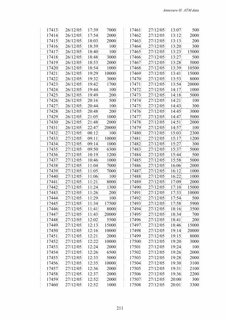
Annexure-II: ATM data
211
17413 26/12/05 17:39 700017414 26/12/05 17:54 200017415 26/12/05 18:03 200017416 26/12/05 18:39 10017417 26/12/05 18:40 10017418 26/12/05 18:48 300017419 26/12/05 18:53 200017420 26/12/05 18:54 100017421 26/12/05 19:29 1000017422 26/12/05 19:32 300017423 26/12/05 19:42 170017424 26/12/05 19:44 10017425 26/12/05 19:49 20017426 26/12/05 20:16 50017427 26/12/05 20:44 10017428 26/12/05 20:48 20017429 26/12/05 21:05 100017430 26/12/05 21:48 200017431 26/12/05 22:47 2000017432 27/12/05 08:12 10017433 27/12/05 09:11 1000017434 27/12/05 09:14 100017435 27/12/05 09:50 630017436 27/12/05 10:19 120017437 27/12/05 10:46 100017438 27/12/05 11:04 700017439 27/12/05 11:05 700017440 27/12/05 11:06 10017441 27/12/05 11:21 800017442 27/12/05 11:24 130017443 27/12/05 11:26 20017444 27/12/05 11:29 10017445 27/12/05 11:34 1750017446 27/12/05 11:41 800017447 27/12/05 11:43 2000017448 27/12/05 12:02 550017449 27/12/05 12:13 1500017450 27/12/05 12:16 1000017451 27/12/05 12:21 200017452 27/12/05 12:22 1000017453 27/12/05 12:24 200017454 27/12/05 12:26 650017455 27/12/05 12:33 500017456 27/12/05 12:35 1000017457 27/12/05 12:36 200017458 27/12/05 12:37 200017459 27/12/05 12:52 200017460 27/12/05 12:52 1000
17461 27/12/05 13:07 50017462 27/12/05 13:12 200017463 27/12/05 13:13 20017464 27/12/05 13:20 30017465 27/12/05 13:23 1500017466 27/12/05 13:27 50017467 27/12/05 13:28 500017468 27/12/05 13:39 1050017469 27/12/05 13:41 1500017470 27/12/05 13:53 800017471 27/12/05 13:54 2000017472 27/12/05 14:17 100017473 27/12/05 14:18 500017474 27/12/05 14:21 10017475 27/12/05 14:43 30017476 27/12/05 14:45 300017477 27/12/05 14:47 500017478 27/12/05 14:51 200017479 27/12/05 14:57 10017480 27/12/05 15:03 230017481 27/12/05 15:17 120017482 27/12/05 15:27 30017483 27/12/05 15:37 500017484 27/12/05 15:44 50017485 27/12/05 15:58 500017486 27/12/05 16:06 200017487 27/12/05 16:12 100017488 27/12/05 16:22 100017489 27/12/05 17:09 200017490 27/12/05 17:10 1500017491 27/12/05 17:33 1000017492 27/12/05 17:54 50017493 27/12/05 17:58 590017494 27/12/05 18:16 350017495 27/12/05 18:34 70017496 27/12/05 18:41 20017497 27/12/05 18:46 1500017498 27/12/05 19:14 2000017499 27/12/05 19:15 800017500 27/12/05 19:20 300017501 27/12/05 19:24 10017502 27/12/05 19:26 200017503 27/12/05 19:28 200017504 27/12/05 19:30 310017505 27/12/05 19:31 210017506 27/12/05 19:36 220017507 27/12/05 20:00 30017508 27/12/05 20:01 3300
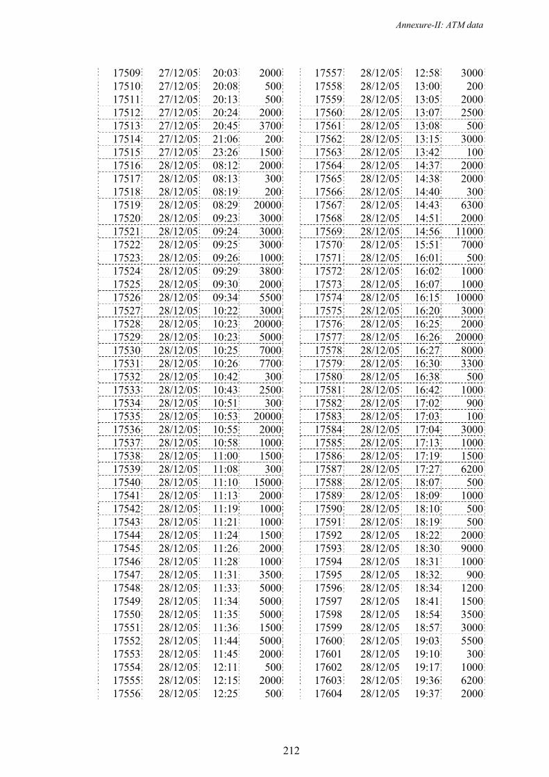
Annexure-II: ATM data
212
17509 27/12/05 20:03 200017510 27/12/05 20:08 50017511 27/12/05 20:13 50017512 27/12/05 20:24 200017513 27/12/05 20:45 370017514 27/12/05 21:06 20017515 27/12/05 23:26 150017516 28/12/05 08:12 200017517 28/12/05 08:13 30017518 28/12/05 08:19 20017519 28/12/05 08:29 2000017520 28/12/05 09:23 300017521 28/12/05 09:24 300017522 28/12/05 09:25 300017523 28/12/05 09:26 100017524 28/12/05 09:29 380017525 28/12/05 09:30 200017526 28/12/05 09:34 550017527 28/12/05 10:22 300017528 28/12/05 10:23 2000017529 28/12/05 10:23 500017530 28/12/05 10:25 700017531 28/12/05 10:26 770017532 28/12/05 10:42 30017533 28/12/05 10:43 250017534 28/12/05 10:51 30017535 28/12/05 10:53 2000017536 28/12/05 10:55 200017537 28/12/05 10:58 100017538 28/12/05 11:00 150017539 28/12/05 11:08 30017540 28/12/05 11:10 1500017541 28/12/05 11:13 200017542 28/12/05 11:19 100017543 28/12/05 11:21 100017544 28/12/05 11:24 150017545 28/12/05 11:26 200017546 28/12/05 11:28 100017547 28/12/05 11:31 350017548 28/12/05 11:33 500017549 28/12/05 11:34 500017550 28/12/05 11:35 500017551 28/12/05 11:36 150017552 28/12/05 11:44 500017553 28/12/05 11:45 200017554 28/12/05 12:11 50017555 28/12/05 12:15 200017556 28/12/05 12:25 500
17557 28/12/05 12:58 300017558 28/12/05 13:00 20017559 28/12/05 13:05 200017560 28/12/05 13:07 250017561 28/12/05 13:08 50017562 28/12/05 13:15 300017563 28/12/05 13:42 10017564 28/12/05 14:37 200017565 28/12/05 14:38 200017566 28/12/05 14:40 30017567 28/12/05 14:43 630017568 28/12/05 14:51 200017569 28/12/05 14:56 1100017570 28/12/05 15:51 700017571 28/12/05 16:01 50017572 28/12/05 16:02 100017573 28/12/05 16:07 100017574 28/12/05 16:15 1000017575 28/12/05 16:20 300017576 28/12/05 16:25 200017577 28/12/05 16:26 2000017578 28/12/05 16:27 800017579 28/12/05 16:30 330017580 28/12/05 16:38 50017581 28/12/05 16:42 100017582 28/12/05 17:02 90017583 28/12/05 17:03 10017584 28/12/05 17:04 300017585 28/12/05 17:13 100017586 28/12/05 17:19 150017587 28/12/05 17:27 620017588 28/12/05 18:07 50017589 28/12/05 18:09 100017590 28/12/05 18:10 50017591 28/12/05 18:19 50017592 28/12/05 18:22 200017593 28/12/05 18:30 900017594 28/12/05 18:31 100017595 28/12/05 18:32 90017596 28/12/05 18:34 120017597 28/12/05 18:41 150017598 28/12/05 18:54 350017599 28/12/05 18:57 300017600 28/12/05 19:03 550017601 28/12/05 19:10 30017602 28/12/05 19:17 100017603 28/12/05 19:36 620017604 28/12/05 19:37 2000

Annexure-II: ATM data
213
17605 28/12/05 19:38 300017606 28/12/05 19:57 1000017607 28/12/05 20:15 50017608 28/12/05 20:20 50017609 28/12/05 20:33 2000017610 28/12/05 20:37 250017611 28/12/05 20:50 200017612 28/12/05 21:05 50017613 28/12/05 21:06 20017614 28/12/05 21:07 50017615 28/12/05 22:03 100017616 28/12/05 22:42 2000017617 29/12/05 08:26 100017618 29/12/05 09:23 100017619 29/12/05 09:34 300017620 29/12/05 09:36 300017621 29/12/05 09:54 30017622 29/12/05 09:56 430017623 29/12/05 10:32 200017624 29/12/05 10:49 290017625 29/12/05 10:51 300017626 29/12/05 11:01 10017627 29/12/05 11:04 300017628 29/12/05 11:05 300017629 29/12/05 11:06 2000017630 29/12/05 11:08 500017631 29/12/05 11:09 500017632 29/12/05 11:12 300017633 29/12/05 11:13 300017634 29/12/05 11:14 200017635 29/12/05 11:18 500017636 29/12/05 11:29 30017637 29/12/05 11:32 800017638 29/12/05 11:34 1500017639 29/12/05 11:46 650017640 29/12/05 11:49 20017641 29/12/05 11:50 700017642 29/12/05 11:55 300017643 29/12/05 11:57 50017644 29/12/05 11:57 50017645 29/12/05 12:11 300017646 29/12/05 12:17 150017647 29/12/05 12:22 2200017648 29/12/05 12:30 200017649 29/12/05 13:19 10017650 29/12/05 13:21 200017651 29/12/05 13:39 20017652 29/12/05 14:35 100
17653 29/12/05 14:43 500017654 29/12/05 14:47 700017655 29/12/05 14:49 20017656 29/12/05 14:52 200017657 29/12/05 15:03 100017658 29/12/05 16:01 800017659 29/12/05 16:19 500017660 29/12/05 16:52 300017661 29/12/05 16:53 100017662 29/12/05 16:58 200017663 29/12/05 17:00 300017664 29/12/05 17:02 20017665 29/12/05 17:10 100017666 29/12/05 17:11 500017667 29/12/05 17:12 200017668 29/12/05 17:14 500017669 29/12/05 17:18 50017670 29/12/05 17:21 30017671 29/12/05 17:26 20017672 29/12/05 17:39 200017673 29/12/05 17:40 50017674 29/12/05 17:42 500017675 29/12/05 17:58 250017676 29/12/05 18:09 50017677 29/12/05 18:18 300017678 29/12/05 18:19 100017679 29/12/05 18:21 100017680 29/12/05 18:27 300017681 29/12/05 18:28 100017682 29/12/05 18:31 500017683 29/12/05 18:34 1000017684 29/12/05 18:38 100017685 29/12/05 18:49 200017686 29/12/05 18:51 720017687 29/12/05 19:00 500017688 29/12/05 19:11 300017689 29/12/05 19:19 350017690 29/12/05 19:21 30017691 29/12/05 19:25 200017692 29/12/05 19:33 100017693 29/12/05 19:35 500017694 29/12/05 19:38 50017695 29/12/05 19:40 10017696 29/12/05 19:44 1000017697 29/12/05 20:13 500017698 29/12/05 20:14 200017699 29/12/05 20:31 300017700 29/12/05 20:36 1000
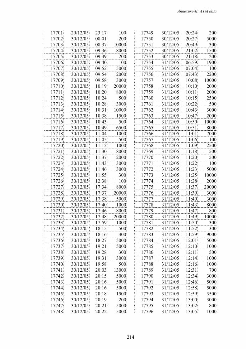
Annexure-II: ATM data
214
17701 29/12/05 23:17 10017702 30/12/05 08:01 20017703 30/12/05 08:37 1000017704 30/12/05 09:36 800017705 30/12/05 09:39 20017706 30/12/05 09:40 10017707 30/12/05 09:52 500017708 30/12/05 09:54 200017709 30/12/05 09:58 300017710 30/12/05 10:19 2000017711 30/12/05 10:20 800017712 30/12/05 10:24 50017713 30/12/05 10:28 300017714 30/12/05 10:31 1000017715 30/12/05 10:38 150017716 30/12/05 10:43 50017717 30/12/05 10:49 650017718 30/12/05 11:04 100017719 30/12/05 11:05 50017720 30/12/05 11:12 100017721 30/12/05 11:30 800017722 30/12/05 11:37 200017723 30/12/05 11:43 300017724 30/12/05 11:46 300017725 30/12/05 11:55 30017726 30/12/05 12:38 10017727 30/12/05 17:34 800017728 30/12/05 17:37 2000017729 30/12/05 17:38 500017730 30/12/05 17:40 100017731 30/12/05 17:46 800017732 30/12/05 17:48 2000017733 30/12/05 17:59 100017734 30/12/05 18:15 50017735 30/12/05 18:16 30017736 30/12/05 18:27 500017737 30/12/05 19:21 500017738 30/12/05 19:28 30017739 30/12/05 19:31 300017740 30/12/05 19:58 50017741 30/12/05 20:03 1300017742 30/12/05 20:15 500017743 30/12/05 20:16 500017744 30/12/05 20:16 500017745 30/12/05 20:18 150017746 30/12/05 20:19 20017747 30/12/05 20:21 500017748 30/12/05 20:22 5000
17749 30/12/05 20:24 20017750 30/12/05 20:27 500017751 30/12/05 20:49 30017752 30/12/05 21:02 150017753 30/12/05 21:18 20017754 31/12/05 06:59 190017755 31/12/05 07:04 10017756 31/12/05 07:43 220017757 31/12/05 10:08 1000017758 31/12/05 10:10 200017759 31/12/05 10:11 200017760 31/12/05 10:15 250017761 31/12/05 10:22 50017762 31/12/05 10:43 300017763 31/12/05 10:47 200017764 31/12/05 10:50 1000017765 31/12/05 10:51 800017766 31/12/05 11:01 700017767 31/12/05 11:06 10017768 31/12/05 11:09 250017769 31/12/05 11:18 50017770 31/12/05 11:20 50017771 31/12/05 11:22 10017772 31/12/05 11:23 500017773 31/12/05 11:25 1000017774 31/12/05 11:28 200017775 31/12/05 11:37 2000017776 31/12/05 11:39 300017777 31/12/05 11:40 300017778 31/12/05 11:43 800017779 31/12/05 11:47 80017780 31/12/05 11:49 1000017781 31/12/05 11:50 30017782 31/12/05 11:52 30017783 31/12/05 11:59 900017784 31/12/05 12:01 500017785 31/12/05 12:10 100017786 31/12/05 12:11 50017787 31/12/05 12:14 100017788 31/12/05 12:16 100017789 31/12/05 12:31 70017790 31/12/05 12:34 300017791 31/12/05 12:46 500017792 31/12/05 12:58 500017793 31/12/05 12:59 350017794 31/12/05 13:00 300017795 31/12/05 13:02 80017796 31/12/05 13:05 1000

Annexure-II: ATM data
215
17797 31/12/05 13:05 50017798 31/12/05 13:14 300017799 31/12/05 13:28 50017800 31/12/05 14:17 500017801 31/12/05 14:29 500017802 31/12/05 14:30 500017803 31/12/05 14:32 500017804 31/12/05 14:33 500017805 31/12/05 15:03 100017806 31/12/05 15:27 250017807 31/12/05 15:55 70017808 31/12/05 17:20 100017809 31/12/05 17:25 1500017810 31/12/05 17:37 2000
17811 31/12/05 17:43 500017812 31/12/05 17:44 200017813 31/12/05 17:47 1000017814 31/12/05 17:53 300017815 31/12/05 18:02 100017816 31/12/05 18:05 100017817 31/12/05 18:21 1000017818 31/12/05 18:23 300017819 31/12/05 18:30 500017820 31/12/05 19:10 1500017821 31/12/05 20:14 1000017822 31/12/05 20:38 50017823 31/12/05 20:58 200017824 31/12/05 21:02 4100
Remark: As total number of hits is 17824, we did not show complete data because of
space. If any one require we can provide it as we have stored as soft copy.