Embed Size (px)
Citation preview
sc4026Exercise Session 7 (with solutions)
Alessandro Abate
Marco Forgione
Delft Center for Systems and Control, TU Delft
October 25, 2012
– Ac.Yr. 2012/13, 1e Sem. Q1 – Exercise Session 7 – sc4026

A. Abate, M. Forgione
Solution to state space models
Find the output response to a step input, where the system
is given by:
X = AX + BU
Y = CX +DU,
where
X(0) =
[1
0
], B =
[1
0
], C =
[1 0
], D = 0,
and where A is [−1 3
0 −4
].
Compute then the steady-state error to a step input, and verify
the correctness of the result by calculating the transfer function
of the model.
Solution:
– Ac.Yr. 2012/13, 1e Sem. Q1 – Exercise Session 7 – sc4026 1

A. Abate, M. Forgione
The output is
Y (t) = CX(t) +DU(t)
= CeAtX(0) + C
∫ t
0
eA(t−τ)
BU(τ)dτ +DU(t).
It is easy to see that eAt =
[e−t e−t − e−4t
0 e−4t
].
Step input means u(t) =
{1, t > 0
0, t = 0.With reference to
the values in the matrices B,C,X(0), we obtain y(t) =
e−t + 1 − e−t = 1. Notice that the non-zero initial condition
“cancels out” the effect of the input.
Thus, the steady-state error to a step input is equal to zero.
Let us compute the relationship, in frequency, between input,initial conditions, and output:
Y (s) = (C(sI − A)−1B +D)U(s) + Ce
At(X(0)− (sI − A)
−1B).
Notice that the effect of the non-zero state X(0) vanishes since
the state matrix A is stable.
The steady-state to a state response can be thus computed
through
[1 0
] [ s+ 1 −3
0 s+ 4
]−1 [1
0
]+ 0 =
1
s+ 1,
– Ac.Yr. 2012/13, 1e Sem. Q1 – Exercise Session 7 – sc4026 2

A. Abate, M. Forgione
so the steady-state is computed by setting s = 0, which gives 1.
This means that the steady-state error to a step input is zero.
2
– Ac.Yr. 2012/13, 1e Sem. Q1 – Exercise Session 7 – sc4026 3
A. Abate, M. Forgione
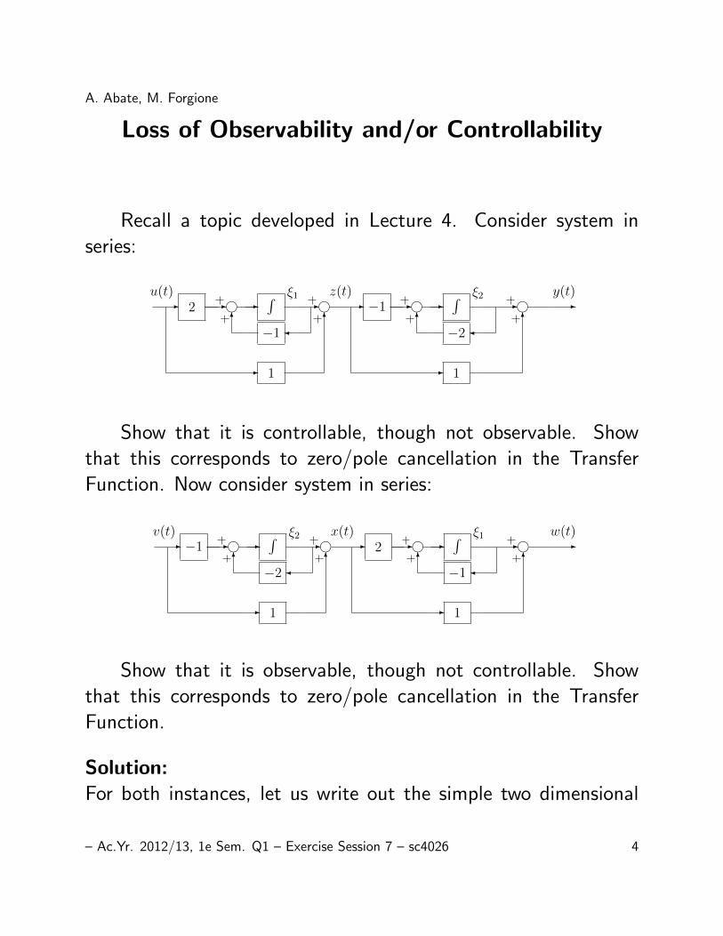
Loss of Observability and/or Controllability
Recall a topic developed in Lecture 4. Consider system in
series:
Stabilizable, detectable 117
Controllable and observable eigenvalues can be relocated by feedback.
In some cases, it is su!cient that the unstable eigenvalues are
controllable and observable, leading to the following weaker concepts
Definition
(A, B) is stabilisable if all!!i(A)
""" Re!i(A) ! 0#
are controllable
(A, C) is detectable if all!!i(A)
""" Re!i(A) ! 0#
are observable
Note that the eigenvalues on the imaginary axis are considered as
unstable.
Controllability/observability 9: pole-zero cancellation 118
s + 3
s + 1! s + 1
s + 2! !
u(s) z(s) y(s)
Simulation diagram (time domain):
$!
$!"1!
"1 " "2 "
1! 1!
!#
! !#
!!#
! !#
!2! !u(t) z(t) y(t)"1 "2
Controllability/observability 9: pole-zero cancellation 119
Diagram uniquely defines (A, B, C,D):
%A B
C D
&=
'()
"1 0 2
"1 "2 "1
1 1 1
*+,
-B AB
.=
%2 "2
"1 0
&rank is 2
%C
CA
&=
%1 1
"2 "2
&rank is 1
Controllable, not completely observable.
Controllability/observability 9: pole-zero cancellation 120
Eigenvectors of !1 = "1, !2 = "2:
m1 =
%1
"1
&m2 =
%0
1
&
%C
CA
&m1 = 0
/ 01 2unobservable
%C
CA
&m2 #= 0
/ 01 2observable
Unobservable eigenvalue !2 = "1 is cancelled by forming transfer
function
C(sI " A)!1B + D =
3s + 3
s + 2
4
Show that it is controllable, though not observable. Show
that this corresponds to zero/pole cancellation in the Transfer
Function. Now consider system in series:
Controllability/observability 9: zero-pole cancellation 121
s + 1
s + 2! s + 3
s + 1! !
v(s) x(s) w(s)
Simulation diagram (time domain)
!!
!!2!
!2 " !1 "
1! 1!
!#
! !#
!!#
! !#
!!1! !v(t) x(t) w(t)!2 !1
Controllability/observability 9: zero-pole cancellation 122
Diagram uniquely defines (A, B, C,D):
"A B
C D
#=
$%&
!1 2 2
0 !2 !1
1 1 1
'()
*B AB
+=
"2 !4
!1 2
#rank=1
"C
CA
#=
"1 1
!1 0
#rank=2
Observable, not completely controllable
Controllability/observability 9: zero-pole cancellation 123
Eigenvectors of "1 = !1, "2 = !2:
m1 =
"1
0
#m2 =
"2
!1
#
m1 /" range*
B AB+
, -. /uncontrollable
m2 " range*
B AB+
, -. /controllable
Uncontrollable eigenvalue " = !1 is cancelled by forming transfer
function
C(sI ! A)!1B + D =
0s + 3
s + 2
1
Minimal order 124
Result
Let R be controllable subspace of (A, B). Let Tc bring (A, B)
to form of (94), then columns 1, 2, . . . , nc of T!1c span R
Let N be unobservable subspace of (A, C). Let To bring (A, C)
to form of (98), then columns no + 1, . . . , n of T!1o span N
In general, Tc and To will be di!erent
Definition
(A, B, C) is of minimal order if (A, B) is controllable and (A, C)
is observable. Then (A, B, C) is called a minimal realisation
Show that it is observable, though not controllable. Show
that this corresponds to zero/pole cancellation in the Transfer
Function.
Solution:For both instances, let us write out the simple two dimensional
– Ac.Yr. 2012/13, 1e Sem. Q1 – Exercise Session 7 – sc4026 4

A. Abate, M. Forgione
state-space representations of the two models, which are both
observable and controllable, interconnect them and show the lack
of either property.
Let us then introduce the transfer functions of the system
components (rather than of the 2-d compositions), and show
the cancellations.
Introducing state variable [ξ1 ξ2]T , input u and output y,
we have:
A =
[−1 0
−1 −2
], B =
[2
−1
],
C =[
1 1], D = [1].
The Kalman controllability matrix is:[2 −2
−1 0
],
which is full rank. Thus, the composition is controllable. However
the observability one is: [1 1
−2 −2
],
which is not full rank. Thus, the composition is not observable.
Given a state-space representation, a transfer function can be
– Ac.Yr. 2012/13, 1e Sem. Q1 – Exercise Session 7 – sc4026 5

A. Abate, M. Forgione
obtained as C(sI − A)−1B + D. The first module has the
following transfer functions:
Gf(s) =s+ 3
s+ 1,
whereas the second
Gs(s) =s+ 1
s+ 2.
You can see that the pole of the first TF cancels with the zero of
the second TF.
Similarly, for the second model, introducing state variable
[ξ1 ξ2]T , input v and output w, we have:
A =
[−1 2
0 −2
], B =
[2
−1
],
C =[
1 1], D = [1].
The Kalman controllability matrix is:[2 −4
−1 2
],
which is not full rank. Thus, the composition is not controllable.
– Ac.Yr. 2012/13, 1e Sem. Q1 – Exercise Session 7 – sc4026 6
A. Abate, M. Forgione
The observability one is: [1 1
−1 0
],
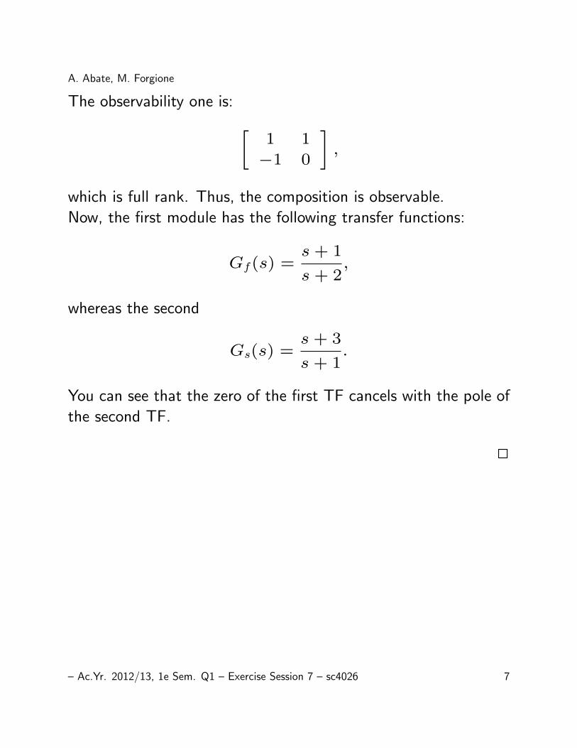
which is full rank. Thus, the composition is observable.
Now, the first module has the following transfer functions:
Gf(s) =s+ 1
s+ 2,
whereas the second
Gs(s) =s+ 3
s+ 1.
You can see that the zero of the first TF cancels with the pole of
the second TF.
2
– Ac.Yr. 2012/13, 1e Sem. Q1 – Exercise Session 7 – sc4026 7

A. Abate, M. Forgione
Controllable Canonical Form from polynomials ofTransfer Function
Consider the following transfer function:
Y (s)
U(s)=
(s+ 10)(s2 + s+ 25)
s2(s+ 3)(s2 + s+ 36).
Give a state-space description of the system in its canonical
controllable form.
Solution:Let us recall some theory to begin with.
Consider a transfer function as a ratio between two polynomials,
as follows:
Y (s)
U(s)=
b1sn−1 + b2s
n−2 + . . .+ bn
sn + a1sn−1 + a2sn−2 + . . .+ an.
There exists a state-space representation of this transfer function
(a.k.a., a realization), which takes the form of the controllable
– Ac.Yr. 2012/13, 1e Sem. Q1 – Exercise Session 7 – sc4026 8

A. Abate, M. Forgione
canonical form, where:
A =
−a1 −a3 . . . −an
1 0 . . . 0...
0 ...
0 . . . 0 1 0
, B =
1
0...
0
0
,C =
[b1 b2 . . . . . . bn
], D = [0].
In MATLAB, this realization is obtained with the command
tf2ss . Notice that in general it is not always possible to
obtain such a realization. (There are sufficient conditions on the
rational functions for that, but we do not discuss them right now.)
Also, notice that this realization is not unique. In particular, we
may be interested to obtain the observable canonical form.
In our instance, we have:
Y (s)
U(s)=
(s+ 10)(s2 + s+ 25)
s2(s+ 3)(s2 + s+ 36)
=s3 + 11s2 + 35s+ 250
s5 + 4s4 + 39s3 + 108s2
=b(s)
a(s).
From this expression, we have that b1 = 0, b2 = 1, b3 =11, b4 = 35, b5 = 250; a1 = 4, a2 = 39, a3 = 108, a4 =
– Ac.Yr. 2012/13, 1e Sem. Q1 – Exercise Session 7 – sc4026 9
A. Abate, M. Forgione
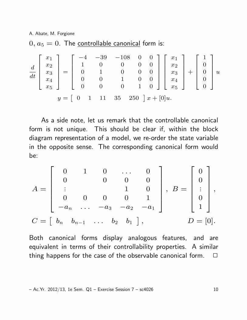
0, a5 = 0. The controllable canonical form is:
d
dt
x1
x2
x3
x4
x5
=
−4 −39 −108 0 01 0 0 0 00 1 0 0 00 0 1 0 00 0 0 1 0
x1
x2
x3
x4
x5
+
10000
uy =
[0 1 11 35 250
]x+ [0]u.
As a side note, let us remark that the controllable canonical
form is not unique. This should be clear if, within the block
diagram representation of a model, we re-order the state variable
in the opposite sense. The corresponding canonical form would
be:
A =
0 1 0 . . . 0
0 0 0 0... 1 0
0 0 0 0 1
−an . . . −a3 −a2 −a1
, B =
0
0...
0
1
,C =
[bn bn−1 . . . b2 b1
], D = [0].
Both canonical forms display analogous features, and are
equivalent in terms of their controllability properties. A similar
thing happens for the case of the observable canonical form. 2
– Ac.Yr. 2012/13, 1e Sem. Q1 – Exercise Session 7 – sc4026 10

A. Abate, M. Forgione
Observer Design for DC Servo
Problem 2: Observer design.
x2 x1
Observer
a2su
a1s
u 1
z2
z
Figure 2: Simple model of a DC Servo system.
Figure 2 shows a block diagram representation of a simple model of a DC servo system: x1 is a voltage signalproportional to the output angular velocity x2 (ie. a tacho signal is not available).
(a) Design a full order observer, with observer gain matrix T given by
T =
!
T1
T2
"
, (3)
for x1 and x2 so that the characteristic polynomial associated with the error dynamics is given by:
!e(s) = s2 + 2!e"es + "2
e (4)
(“Design” means write the equations for the observer, with expressions for gains T1 and T2.)
(b) Now, the observer is a system with inputs u and x1, and outputs z1 and z2. Thus, there are four possibletransfer functions between inputs and outputs – these may be included as elements in a 2!2 matrix. Evaluatethe following matrix of transfer functions M(s) between the inputs to the observer u and x1, and its outputsz1 and z2:
M(s) =
!
z1(s)/u(s) z1(s)/x1(s)z2(s)/u(s) z2(s)/x1(s)
"
(5)
as a function of gains T1 and T2, as well as system parameters a1 and a2.
(c) Now determine M(s) as T2 " #. Discuss the meaning of the result.
Problem 3: Observer design.
x1 x2
z1
uinput
velocityobserved variable
observeroutput
observer
1s 2+s
2 s
Figure 3: Velocity Observation System.
Figure 3 shows a velocity observation system where x1 is the velocity to be observed. An observer is to beconstructed to track x1, using u and x2 as inputs. The variable x2 is obtained from x1 through a sensor havingthe known transfer function
2 $ s
2 + s(6)
2
The Figure above shows a block diagram representation of a
simple model of a DC servo system. The variable x1 is a voltage
signal that corresponds to the output y, whereas x2 is the angular
velocity.
1. Design an observer, with observer gain matrix L = [l1 l2]T ,
for the variables x1, x2, and such that the characteristic
polynomial associated with the error dynamics is given by:
∆(s) = s2
+ 2ζωs+ ω2.
2. The observer is a system with inputs u and x1, and with
outputs z1 and z2. Thus, there are four possible transfer
functions between inputs and outputs these may be included
as elements in a 2× 2 matrix. Evaluate the following matrix
– Ac.Yr. 2012/13, 1e Sem. Q1 – Exercise Session 7 – sc4026 11

A. Abate, M. Forgione
of transfer functions M(s) between the inputs to the observer
u and x1, and its outputs z1 and z2
M(s) =
[Z1(s)
U(s)
Z1(s)
X1(s)Z2(s)
U(s)
Z2(s)
X1(s)
],
as a function of gains l1 and l2, as well as of the system
parameters a1, a2.
3. Determine M(s) as l2 → ∞. Discuss the meaning of the
result.
Solution:We have:
X1(s) =a2
sX2(s) ⇒ x1(t) = a2x2(t)
X2(s) =a1
sU(s) ⇒ x2(t) = a1u(t)
y(t) = x1(t)
The state-space model follows:
d
dt
[x1
x2
]=
[0 a2
0 0
] [x1
x2
]+
[0
a1
]u
y =[
1 0] [ x1
x2
]+ [0]u.
– Ac.Yr. 2012/13, 1e Sem. Q1 – Exercise Session 7 – sc4026 12

A. Abate, M. Forgione
Let us introduce an observer matrix L =
[l1l2
]. The closed-
loop matrix for the estimator is
A− LC =
[−l1 a2
−l2 0
].
Let us compute the characteristic polynomial:
det(sI − (A− LC)) = s(s+ l1) + a2l2,
which is then equated to the desired characteristic polynomial,
thus obtaining:
l1 = 2ζω, l2 =ω2
a2
.
Let us now look closer at the observer, with variable z =
[z1 z2]T : ˙z = Az + Bu + L(y − y) = Az + Bu + L(y −
Cz) = (A−LC)z+[B L][u y]T , where y = x1. We obtain:
d
dt
[z1
z2
]=
[−l1 a2
−l2 0
] [z1
z2
]+
[0 l1a1 l2
] [u
y
]y =
[1 0
0 1
] [z1
z2
].
– Ac.Yr. 2012/13, 1e Sem. Q1 – Exercise Session 7 – sc4026 13

A. Abate, M. Forgione
The transfer function can be directly found as follows:
M(s) = C(sI − A)−1B +D
=
[1 0
0 1
] [s+ l1 −a2
l2 s
]−1 [0 l1a1 l2
]=
1
s2 + l1s+ a2l2
[a1a2 sl1 + a2l2
a1(s+ l1) sl2
].
If l2 →∞, we have:
liml2→∞
M(s) =
[0 1
0 s/a2
].
Since l2 = ω2/a2, whenever l2 → ∞, then ω2 → ∞. The
speed of the estimator thus increases in speed and its error
converges to zero infinitely fast at the limit. In the long run, we
expect z1(t) → x1(t), z2(t) → x2(t) =x1(t)
a2, and that the
effect of the input on the estimate is null.
2
– Ac.Yr. 2012/13, 1e Sem. Q1 – Exercise Session 7 – sc4026 14

A. Abate, M. Forgione
Heading Controller for Aircraft Ground Control
EECS 128 Introduction to Control Design Techniques
Problem Set 3
Professor C. TomlinDepartment of Electrical Engineering and Computer Sciences
University of California at Berkeley, Fall 2008Issued 10/2; Due 10/9
Problem 1: Heading controllers for ground control of aircraft. A top view of the tricycle landing gear
!a
"
L
V
Figure 1: Tricycle landing gear top view.
for a small unmanned aerial vehicle is shown in Figure 1. Consider the case in which the vehicle is movingwith constant forward velocity V (achieved by an input motor thrust, not shown here). The only input wewould like to consider here is the heading actuator !a, which a!ects the heading ". The dynamics betweenheading actuator and heading, for small angle changes, can be modeled as:
"(s) =V
L
1
s(#s + 1)!a(s)
(a) Design a controller for this system, so that a given step reference heading "ref = 1 is achieved with nosteady state error.
(b) Design a controller for this system, so that a given step reference heading rate $ref = "ref = 1 (corre-sponding to a changing heading) is achieved with no steady state error.
Problem 2. Root locus design.
G(s)R YK(s)
Figure 2: Unity Feedback System with proportional controller K(s), plant G(s)
Consider the unity feedback system of Figure 2 with G(s) = 1s(s+1) . You would like to have closed loop poles
1
The above figure displays a top view of a tricycle landing
gear of an aircraft. Consider the case in which the vehicle is
moving with constant forward velocity V (achieved by an input
motor thrust, which is not shown here). The only input we would
like to consider here is the heading actuator δa, which affects the
heading ψ. The dynamics between heading actuator and heading,
for small angle changes, can be modeled as
Ψ(s) =V
L
1
s(τs+ 1)∆a(s),
– Ac.Yr. 2012/13, 1e Sem. Q1 – Exercise Session 7 – sc4026 15

A. Abate, M. Forgione
where in the formula we have denoted with capitals letters the
respective Laplace transforms, and where V, L, τ > 0.
1. Write a block diagram representation of the feedback loop
that presents a controller (call it C(s)) and the system block
with input δa and output ψ. The block diagram should
also encompass a reference signal. (If necessary, you can get
inspiration from the first Section of Chapter 9 in the A.M.)
2. Based on this representation, design a controller (the simplest
possible) for this system, so that a given step reference heading
ψref = 1 is achieved with no steady state error. (In other
words, apply a step input at the reference and make sure to
get zero steady state error.)
3. Furthermore, design a controller for this system (again, the
simplest possible), so that a given step reference heading rate
ωref = ψref = 1 (corresponding to a change in the heading)
is achieved with no steady state error.
Solution:The block diagram appears on page 268 of the A.M. book, in
Figure 9.1 a), where P (s) = VL
1s(τs+1) and r = ψref is the
reference signal.
Let us call G(s) = Ψ(s)/∆a(s) = VL
1s(τs+1). Given a
controller C(s), the relationship between ψ and ψref can be
– Ac.Yr. 2012/13, 1e Sem. Q1 – Exercise Session 7 – sc4026 16

A. Abate, M. Forgione
obtained as follows:
Ψ(s)
Ψref(s)=
C(s)G(s)
1 + C(s)G(s).
The steady-state of this transfer function is C(0)G(0)1+C(0)G(0), thus its
error (w.r.t. ψref = 1) is
1−C(0)G(0)
1 + C(0)G(0)=
1
1 + C(0)G(0)
=1
1 + C(s)VL1
s(τs+1)
∣∣∣∣∣s=0
The requirement is thus
1
1 + C(s)VL1
s(τs+1)
∣∣∣∣∣s=0
= 0,
which can be simply achieved by choosing C(s) = C, where C
is a non-zero gain.
The second instance can be obtained by replicating the block
diagram above, and adding a derivative at the output of the block
described by G(s), thus relating Ψ(s) with its derivative sΨ(s).
The transfer function relating ∆a(s) to the derivative of Ψ(s) is
thus sG(s) = VL
1(τs+1). Reasoning along the previous lines, we
– Ac.Yr. 2012/13, 1e Sem. Q1 – Exercise Session 7 – sc4026 17

A. Abate, M. Forgione
get to the following requirement
1
1 + C(s)VL1
(τs+1)
∣∣∣∣∣s=0
= 0,
which can be simply achieved by choosing C(s) = C/s, which
is a simple integrator with gain C.
2
– Ac.Yr. 2012/13, 1e Sem. Q1 – Exercise Session 7 – sc4026 18
A. Abate, M. Forgione
Observer Design Problem
Problem 2: Observer design.
x2 x1
Observer
a2su
a1s
u 1
z2
z
Figure 2: Simple model of a DC Servo system.
Figure 2 shows a block diagram representation of a simple model of a DC servo system: x1 is a voltage signalproportional to the output angular velocity x2 (ie. a tacho signal is not available).
(a) Design a full order observer, with observer gain matrix T given by
T =
!
T1
T2
"
, (3)
for x1 and x2 so that the characteristic polynomial associated with the error dynamics is given by:
!e(s) = s2 + 2!e"es + "2
e (4)
(“Design” means write the equations for the observer, with expressions for gains T1 and T2.)
(b) Now, the observer is a system with inputs u and x1, and outputs z1 and z2. Thus, there are four possibletransfer functions between inputs and outputs – these may be included as elements in a 2!2 matrix. Evaluatethe following matrix of transfer functions M(s) between the inputs to the observer u and x1, and its outputsz1 and z2:
M(s) =
!
z1(s)/u(s) z1(s)/x1(s)z2(s)/u(s) z2(s)/x1(s)
"
(5)
as a function of gains T1 and T2, as well as system parameters a1 and a2.
(c) Now determine M(s) as T2 " #. Discuss the meaning of the result.
Problem 3: Observer design.
x1 x2
z1
uinput
velocityobserved variable
observeroutput
observer
1s 2+s
2 s
Figure 3: Velocity Observation System.
Figure 3 shows a velocity observation system where x1 is the velocity to be observed. An observer is to beconstructed to track x1, using u and x2 as inputs. The variable x2 is obtained from x1 through a sensor havingthe known transfer function
2 $ s
2 + s(6)
2
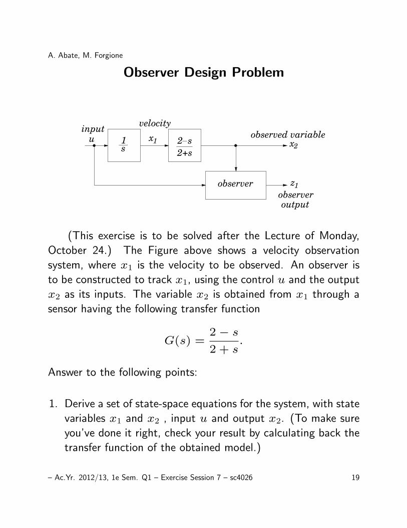
(This exercise is to be solved after the Lecture of Monday,
October 24.) The Figure above shows a velocity observation
system, where x1 is the velocity to be observed. An observer is
to be constructed to track x1, using the control u and the output
x2 as its inputs. The variable x2 is obtained from x1 through a
sensor having the following transfer function
G(s) =2− s2 + s
.
Answer to the following points:
1. Derive a set of state-space equations for the system, with state
variables x1 and x2 , input u and output x2. (To make sure
you’ve done it right, check your result by calculating back the
transfer function of the obtained model.)
– Ac.Yr. 2012/13, 1e Sem. Q1 – Exercise Session 7 – sc4026 19

A. Abate, M. Forgione
Plot the poles and the zeros of the transfer function in
MATLAB. Also, represent its Bode plot with MATLAB.
2. Design an observer with states z1 and z2 to track respectively
x1 and x2. Choose both observer eigenvalues to be at −4.
Write out the state space equations for the observer.
3. Derive the combined state-space equations for the system
composed of the model and of the observer. To do so, consider
four state variables x1, x2, e1 = x1 − z1, e2 = x2 − z2.
Select u as the input and z1 as the output. Is the composed
model controllable and/or observable? If meaningful, try to
give physical reasons for any of the states being uncontrollable
or unobservable.
4. What is the transfer function relating u to z1? (Explain your
result.)
Solution:We have:
X1(s) =1
sU(s)⇒x1(t) = u(t)
X2(s) =2− s2 + s
X1(s)⇒(2 + s)X2(s) = (2− s)X1(s)
⇒x2(t) + 2x2(t) = −x1(t) + 2x1(t)
⇒x2(t) = 2x1(t)− 2x2(t)− u(t)
y(t) = x2(t)
– Ac.Yr. 2012/13, 1e Sem. Q1 – Exercise Session 7 – sc4026 20
A. Abate, M. Forgione
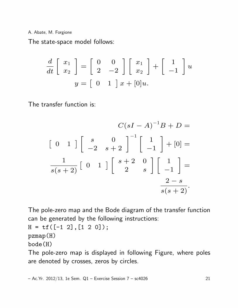
The state-space model follows:
d
dt
[x1
x2
]=
[0 0
2 −2
] [x1
x2
]+
[1
−1
]u
y =[
0 1]x+ [0]u.
The transfer function is:
C(sI − A)−1B +D =
[0 1
] [ s 0
−2 s+ 2
]−1 [1
−1
]+ [0] =
1
s(s+ 2)
[0 1
] [ s+ 2 0
2 s
] [1
−1
]=
2− ss(s+ 2)
.
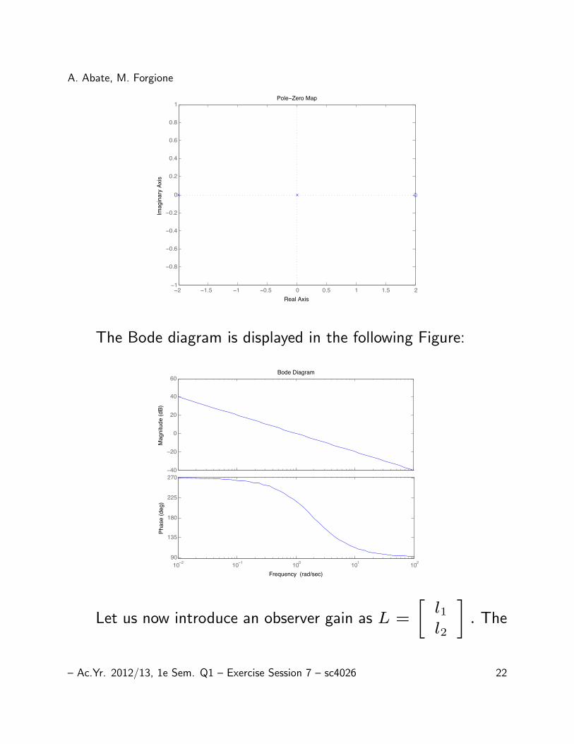
The pole-zero map and the Bode diagram of the transfer function
can be generated by the following instructions:
H = tf([-1 2],[1 2 0]);
pzmap(H)
bode(H)
The pole-zero map is displayed in following Figure, where poles
are denoted by crosses, zeros by circles.
– Ac.Yr. 2012/13, 1e Sem. Q1 – Exercise Session 7 – sc4026 21
A. Abate, M. Forgione
−2 −1.5 −1 −0.5 0 0.5 1 1.5 2−1
−0.8
−0.6
−0.4
−0.2
0
0.2
0.4
0.6
0.8
1Pole−Zero Map
Real Axis
Imag
inar
y Ax
is
The Bode diagram is displayed in the following Figure:
−40
−20
0
20
40
60
Mag
nitu
de (d
B)
10−2 10−1 100 101 10290
135
180
225
270
Phas
e (d
eg)
Bode Diagram
Frequency (rad/sec)
Let us now introduce an observer gain as L =
[l1l2
]. The
– Ac.Yr. 2012/13, 1e Sem. Q1 – Exercise Session 7 – sc4026 22

A. Abate, M. Forgione
closed-loop matrix for the observer is
A− LC =
[0 −l12 −(l2 + 2)
].
Let us compute the characteristic polynomial:
det(sI − (A− LC)) = s2
+ s(l2 + 2) + 2l1.
We can assign the eigenvalues of the observer to the point −4
by choosing
l1 = 8, l2 = 6.
The state space equations for the observer, with variable z =
[z1 z2]T , are:
z = (A− LC)z + [B|L]
[u
y
], y = z2;
d
dt
[z1
z2
]=
[0 −8
2 −8
] [z1
z2
]+
[1 8
−1 6
] [u
y
]y = [0 1]
[z1
z2
].
Let us introduce the error e = x − z, and its dynamics
e = (A − LC)e, which are to be considered along with the
– Ac.Yr. 2012/13, 1e Sem. Q1 – Exercise Session 7 – sc4026 23
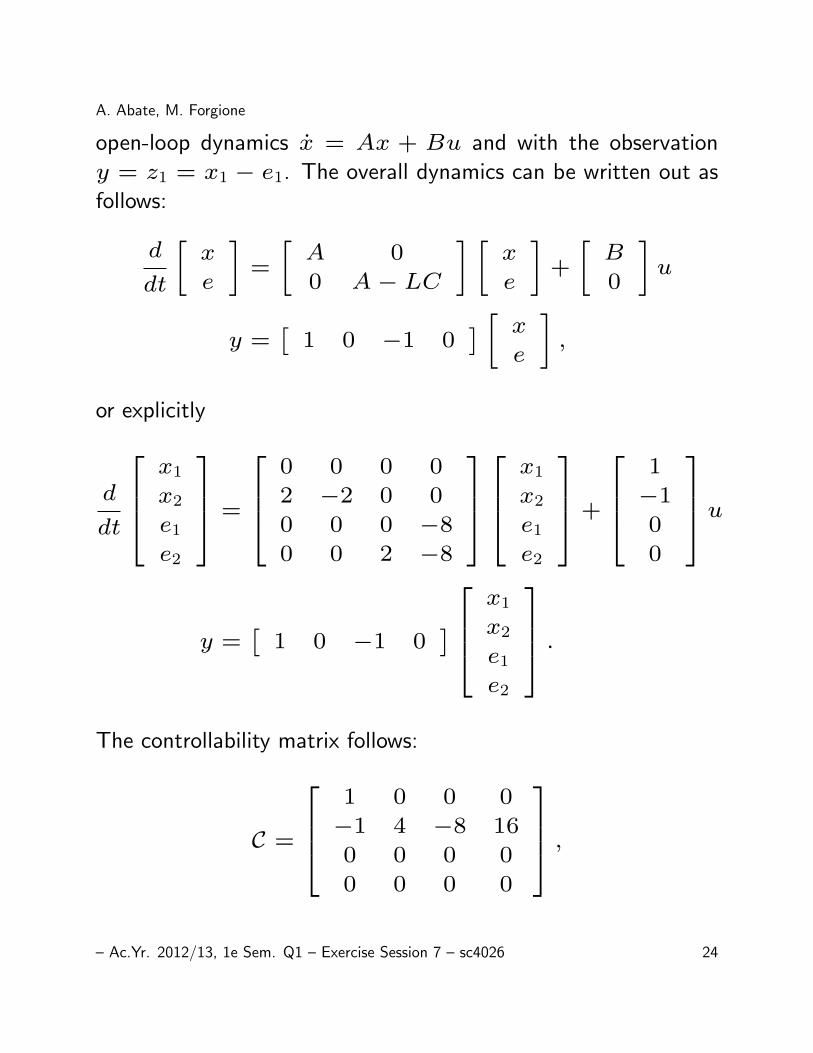
A. Abate, M. Forgione
open-loop dynamics x = Ax + Bu and with the observation
y = z1 = x1 − e1. The overall dynamics can be written out as
follows:
d
dt
[x
e
]=
[A 0
0 A− LC
] [x
e
]+
[B
0
]u
y =[
1 0 −1 0] [ x
e
],
or explicitly
d
dt
x1
x2
e1
e2
=
0 0 0 0
2 −2 0 0
0 0 0 −8
0 0 2 −8
x1
x2
e1
e2
+
1
−1
0
0
u
y =[
1 0 −1 0]
x1
x2
e1
e2
.The controllability matrix follows:
C =
1 0 0 0
−1 4 −8 16
0 0 0 0
0 0 0 0
,
– Ac.Yr. 2012/13, 1e Sem. Q1 – Exercise Session 7 – sc4026 24

A. Abate, M. Forgione
so that
rank(C) = 2 < 4,
which enables us to conclude that the model is uncontrollable.
More precisely, it is so over the error states e1, e2, since they are
bound to decay to zero, regardless of the control effort.
The observability matrix follows:
O =
1 0 −1 0
0 0 0 8
0 0 16 −64
0 0 −128 384
so that
rank(O) = 3 < 4,
which enables us to conclude that the model is unobservable. In
fact, the observer is only estimating values of x1, not of x2.
The transfer function relating u to z1 can be directly derived
– Ac.Yr. 2012/13, 1e Sem. Q1 – Exercise Session 7 – sc4026 25

A. Abate, M. Forgione
as:
C(sI − A)−1B +D
=[
1 0 −1 0]
s 0 0 0−2 s+ 2 0 00 0 s 80 0 −2 s+ 8
−1
1−100
=
1
s.
In fact, we expect that z1 → x1 = 1su.
2
– Ac.Yr. 2012/13, 1e Sem. Q1 – Exercise Session 7 – sc4026 26