Embed Size (px)
Citation preview
SCAIL-Agriculture: User guide
Sniffer ER26 March / 2014

Contents 1. Introduction .................................................................................................................................... 3
1.1. Legislative background ........................................................................................................ 3
1.2. Emission sources and impacts ............................................................................................ 5
1.3. Environmental Assessment Levels, Critical Loads, Critical Levels ....................................... 6
1.4. Meteorology........................................................................................................................ 7
2. The SCAIL-Agriculture Web System ................................................................................................. 8
2.1. SCAIL-Agriculture decision flow chart ................................................................................. 8
2.2. Filling out the Form ........................................................................................................... 10
2.3. Interpreting the Results .................................................................................................... 21
Appendix 1: Typical Meteorological Year Wind Roses ...................................................................... 24
Appendix 2: Ammonia Emission Factors for Cattle ........................................................................... 46
SCAIL-Agriculture: User Guide, March 2014 2

1. Introduction
Simple Calculation of Atmospheric Impact Limits from Agricultural Sources (SCAIL-Agriculture) is a screening tool for assessing the impact from pig and poultry farms on human health and on semi-natural areas like SSSIs and SACs. The model provides an estimate of the amount of acidity and nitrogen deposited as a consequence of ammonia emissions from a farm as well as predictions of air concentrations of ammonia (NH3), odour and particulate matter with an aerodynamic diameter of less than 10 microns (PM10). These values can then be used to assess whether impact limits for human health or habitats are exceeded or not. Please note that the updated version of SCAIL-Agriculture includes a module that provides an estimation of PM10 concentrations. The module is currently under development in consultation with the regulatory authorities, and should only be used to provide an indicative assessment for PM10. The SCAIL-Agriculture user guide provides information on the Industrial Emissions Directive (IED), critical loads and the model, as well as providing a walk-through of the system itself. You will be shown how to complete a query using the web form and how to interpret the results.
1.1. Legislative background
Industrial Emissions Directive - Intensive agriculture is covered under the Environmental Permitting Regulations (in England and Wales); Pollution Prevention and Control (Scotland) Regulations 2012; Pollution Prevention and Control (Industrial Emissions) Regulations (Northern Ireland) 2013 ('The Regulations'); and, Environmental Protection Agency (Industrial Emissions) (Licensing) Regulations Republic of Ireland) 2013 for the rearing of poultry and pigs. There are three main activities that are included in the regulations, for installations with more than:
i) 40,000 places for poultry, including ducks and turkeys; ii) 2,000 places for production pigs (over 30 kilogrammes); or iii) 750 places for sows
For the three situations above, there is also a requirement to look at the different emission sources of NH3 that are occurring within these types of installation - namely emissions from housing, storage and land spreading. On an environmental permit application form, and on the SCAIL web site, you will be asked to fill out all the sources involved in your farming operation that contribute to NH3 emissions. Further detailed information on IED can be found on the APIS IED Directive page. The following links will direct the user to the relevant guidance specific to the agency regulating the installation. England: http://www.environment-agency.gov.uk/business/sectors/40069.aspx; Wales: http://naturalresourceswales.gov.uk/apply-buy-report/apply-buy-grid/installations/intensive-farming/ Scotland: http://www.sepa.org.uk/air/process_industry_regulation/pollution_prevention__control/intensive_agriculture.aspx: Northern Ireland: http://www.doeni.gov.uk/niea/pollution-home/ippc/ippc_farmregs/application_forms_and_guidance.htm; Republic of Ireland: http://www.epa.ie/pubs/forms/lic/ipc/#d.en.46362.
SCAIL-Agriculture: User Guide, March 2014 3

If there is the potential for deposition to have an impact on a site with a conservation designation [e.g. Special Area of Conservation (SAC) or in the UK an Area/Site of Special Scientific Interest (ASSI/SSSI)] then this potential impact needs to be considered. PM10 legislation - Air quality regulation within the EU is based upon the Ambient Air Quality Directive (2008/50/EC) and Directive 2004/107/EC, which set limits for concentrations of pollutants in outdoor air. These are promulgated in national legislation. Air quality is a devolved matter, though the UK government leads on international and European legislation. Administrations in Scotland, Wales and Northern Ireland are responsible for their own air quality policy and legislation. The Air Quality (Standards) Regulations 2010 transpose into English law the requirements of Directives 2008/50/EC and 2004/107/EC on ambient air quality. Equivalent regulations have been made by the devolved administrations in Scotland, Wales and Northern Ireland. The equivalent in the Republic of Ireland is the Air Quality Standards Regulations 2011. Odours - The Environmental Permitting Regulations require the control of pollution including odour. In addition, action on odours can be taken under Section 80 of The Environmental Protection Act 1990 in cases where a statutory nuisance is found to exist. Whether or not odour constitutes a statutory nuisance depends on several factors, including:
• severity • duration • frequency and • whether it interferes with the "average" person's reasonable enjoyment of their property.
In other words, an unpleasant odour in someone's garden in the winter that does not enter their house would not constitute a statutory nuisance as the "average" person would not be expected to spend significant periods of time in their garden during cold weather. However, during warmer weather they are more likely to be in the garden and therefore the same odour would be more likely to constitute a statutory nuisance. A Public Inquiry at Newbiggin-on-Sea established that the 98th percentile of hourly concentrations provided a suitable surrogate for determining an odour nuisance. Typically concentrations above between 1 and 5 Odour Units per cubic meter of air when evaluated as the 98th percentile of hourly values would be determined to result in odour pollution. Horizontal Guidance from the Environment Agency for England, Wales, Scotland and Northern Ireland and the Odour Impact Assessment Guidance for EPA Licensed Sites for the Republic of Ireland provides further details on the assessment of odour issues for regulatory purposes.
Further, guidance can be found at:
http://www.scottishairquality.co.uk | http://www.sepa.org.uk | http://www.apis.ac.uk | http://www.environment-agency.gov.uk |http://naturalresourceswales.gov.uk | http://www.epa.ie | http://www.doeni.gov.uk.
SCAIL-Agriculture: User Guide, March 2014 4
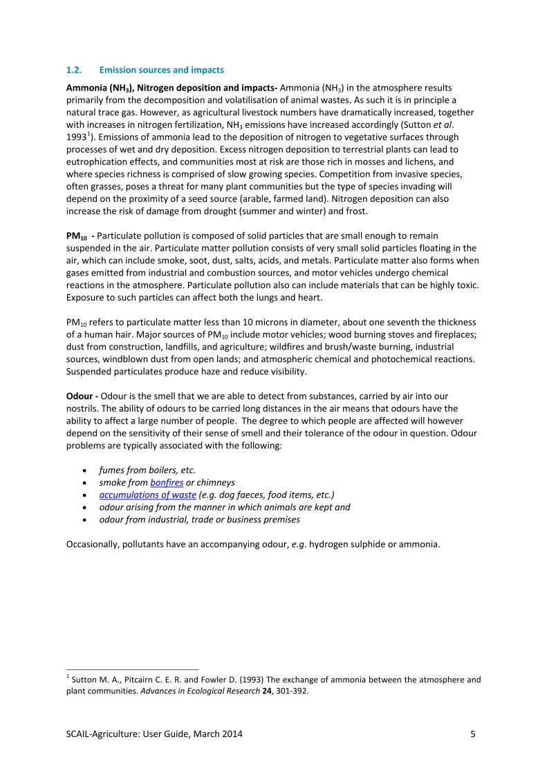
1.2. Emission sources and impacts
Ammonia (NH3), Nitrogen deposition and impacts- Ammonia (NH3) in the atmosphere results primarily from the decomposition and volatilisation of animal wastes. As such it is in principle a natural trace gas. However, as agricultural livestock numbers have dramatically increased, together with increases in nitrogen fertilization, NH3 emissions have increased accordingly (Sutton et al. 19931). Emissions of ammonia lead to the deposition of nitrogen to vegetative surfaces through processes of wet and dry deposition. Excess nitrogen deposition to terrestrial plants can lead to eutrophication effects, and communities most at risk are those rich in mosses and lichens, and where species richness is comprised of slow growing species. Competition from invasive species, often grasses, poses a threat for many plant communities but the type of species invading will depend on the proximity of a seed source (arable, farmed land). Nitrogen deposition can also increase the risk of damage from drought (summer and winter) and frost. PM10 - Particulate pollution is composed of solid particles that are small enough to remain suspended in the air. Particulate matter pollution consists of very small solid particles floating in the air, which can include smoke, soot, dust, salts, acids, and metals. Particulate matter also forms when gases emitted from industrial and combustion sources, and motor vehicles undergo chemical reactions in the atmosphere. Particulate pollution also can include materials that can be highly toxic. Exposure to such particles can affect both the lungs and heart. PM10 refers to particulate matter less than 10 microns in diameter, about one seventh the thickness of a human hair. Major sources of PM10 include motor vehicles; wood burning stoves and fireplaces; dust from construction, landfills, and agriculture; wildfires and brush/waste burning, industrial sources, windblown dust from open lands; and atmospheric chemical and photochemical reactions. Suspended particulates produce haze and reduce visibility. Odour - Odour is the smell that we are able to detect from substances, carried by air into our nostrils. The ability of odours to be carried long distances in the air means that odours have the ability to affect a large number of people. The degree to which people are affected will however depend on the sensitivity of their sense of smell and their tolerance of the odour in question. Odour problems are typically associated with the following:
• fumes from boilers, etc. • smoke from bonfires or chimneys • accumulations of waste (e.g. dog faeces, food items, etc.) • odour arising from the manner in which animals are kept and • odour from industrial, trade or business premises
Occasionally, pollutants have an accompanying odour, e.g. hydrogen sulphide or ammonia.
1 Sutton M. A., Pitcairn C. E. R. and Fowler D. (1993) The exchange of ammonia between the atmosphere and plant communities. Advances in Ecological Research 24, 301-392.
SCAIL-Agriculture: User Guide, March 2014 5

1.3. Environmental Assessment Levels, Critical Loads, Critical Levels
For many substances which are released to air Environmental Quality Standards have not been defined. Where the necessary criteria are absent then the Regulators have adopted interim values known as Environmental Assessment Levels (EALs). The EAL is the concentration of a substance which in a particular environmental medium the Regulators regard as a comparator value to enable a comparison to be made between the environmental effects of different substances in that medium and between environmental effects in different media and to enable the summation of those effects. PM10 are governed by ambient air quality standards set out in the Air Quality (Standards) Regulations 2010. In England, Wales, and Ireland for PM10, the daily average concentration limit is 50 µg/m3, not to be exceeded more than 35 times a calendar year. For Scotland the PM10 daily average concentration limit is 50 µg/m3, not to be exceeded more than 7 times a calendar year. Critical Loads/levels are the threshold level for the deposition or concentration of a pollutant above which harmful indirect effects can be shown on a habitat or species, according to current knowledge. Additional deposition above the Critical Load/Level is termed Critical Load/Level Exceedance. For agricultural practices we are primarily interested in the critical loads for nitrogen and acidity and the critical level for ammonia (NH3) since emissions from livestock farming lead to increased pollutant loads which could cause harmful effects. The impact of excess nitrogen deposition is always quoted in Kg of nitrogen per hectare per year (Kg N/ha/yr) whilst acid deposition is quoted in Kg of hydrogen ion equivalents (K Eq H+) per hectare per year (K Eq H+/ha /yr). Further information on critical loads can be found at: www.apis.ac.uk/overview/issues/overview_Cloadslevels.htm. Critical levels for ammonia are quoted in µg/m3 and have been set for lichens/bryophytes and other vegetation.
SCAIL-Agriculture: User Guide, March 2014 6

1.4. Meteorology
The SCAIL-Agriculture screening model uses an approach that uses data from nearby meteorological stations. The Typical Meteorological Year approach is used to derive meteorological data to best represent the long-term dataset based on the similarity of the annual wind direction distribution to the long-term average (five year). Similarity of long-term wind direction distributions of nearby stations has been used to reduce the number of meteorological stations used. The 30 stations included in the model for the UK are shown in Figure 1a, and the 11 stations for the Republic of Ireland are shown in Figure 1b.
a: 30 Meteorological Station used in SCAIL-Agriculture for the UK
b: 11 Meteorological Station used in SCAIL-Agriculture for the Republic of Ireland Figure 1 Meteorological Station used in SCAIL-Agriculture
SCAIL-Agriculture: User Guide, March 2014 7

2. The SCAIL-Agriculture Web System
This section provides a brief walk-through of the system and will guide you through the form filling exercise and interpretation of the results.
2.1. SCAIL-Agriculture decision flow chart
Figure 2 shows the flow diagram of the SCAIL agriculture tool and the decisions that may be taken in carrying out an environmental assessment. Since the tool compares a number of metrics for habitats or human health, obtaining no exceedance on all limits may be difficult. Where environmental standards are already exceeded by the background or the new installation results in an exceedance you should consult the relevant regulatory guidance for further action. In addition, for emissions of ammonia where a sensitive receptor is located within 250 metres of the installation the following guidance must be followed:
• For intensive farming sites that are regulated under the Environmental Permitting Regulations (EPR) in England and Wales (PPC permitted sites in Scotland, IPPC in Northern Ireland) and with distances to the nearest sensitive receptor of less than 250m, applicants must go straight to undertaking detailed modelling.
• For non-EPR (PPC / IPPC) sites with distances to the nearest sensitive receptor between 100-250m, SCAIL can be used and then advice must be sought from the regulator for clarification on whether detailed modelling is required.
• For sites with distances to the nearest sensitive receptor of less than 100m, detailed modelling will be required.
SCAIL-Agriculture: User Guide, March 2014 8

Figure 2: SCAIL Agriculture flow chart
SCAIL-Agriculture: User Guide, March 2014 9

2.2. Filling out the Form
Throughout the SCAIL-Agriculture web system the user is provided with guidance notes by using the information icon ( ). By clicking the mouse on the icon (see Figure 3) text is displayed in the grey box on the right of the form giving guidance on the relevant input field.
Figure 3: How to use the guidance info tool
Entering Input Data:
All the information needed to run the model is entered on the web form. However, if you have saved input data from a previous run, this can be loaded by clicking on the Load Input Data button at the top-right of the form. This will bring up a window where the input file can be selected and loaded (Figure 4). This will populate the form with the saved input data, ready to edit or run.
Figure 4: Specifying file for loading input data Project Details & Run Mode: In the Project Notes box you can enter details on the sources to be modelled and the type of run being carried out, e.g. ‘worst case’ or ‘realistic’. This information is copied onto the output screen and also to any output files saved (Figure 5). For the Project Run Mode, either Conservative or Realistic Met can be chosen (Figure 5). Realistic Met will use the actual position of the habitat site, and Conservative Met will rotate the habitat site so that it is in the prevailing wind direction for the meteorological file being used and
SCAIL-Agriculture: User Guide, March 2014 10

hence receive the highest amount of pollutant concentration and deposition. The ‘Conservative Met’ assumption can help to ensure that the effects of local wind fields are captured. However, the method works best for situations where there are either single sources or sources are closely grouped, and care needs to be taken with sources that are widely spaced apart. For situations where a large number of sources are being modelled across a wide geographical area the modeller should use the actual source position as applied through the “realistic met” option. As a general rule run the model for both ‘Conservative Met’ and ‘Realistic Met’ situations. Where SCAIL-Agriculture results are to be reported to the relevant regulatory authority, results must be produced using the Conservative Met run mode. SCAIL-Agriculture can be used in either mode as a guide for non-regulatory purposes such as exploratory investigations for planning, pre-application or research. Details of the meteorological sites included in SCAIL-Agriculture can be seen in Appendix 1. The prevailing wind direction at each of the meteorological sites is listed in Table A1.1, ‘Wind Direction (degrees)’. The following examples illustrate the use of the ‘Conservative Met’ option. The left hand and centre figures illustrate that the rotation of the receptor locations into the prevailing wind direction works well when sources are located close to Installation number 1. The methodology does not work well though when sources are distant from Installation number 1 as shown in the right hand figure. For this reason, the use of SCAIL-Agriculture is not suitable for regulatory screening of sites with multiple installations or dispersed sources, and the relevant Regulatory Authority should be contacted for advice.
SCAIL-Agriculture: User Guide, March 2014 11
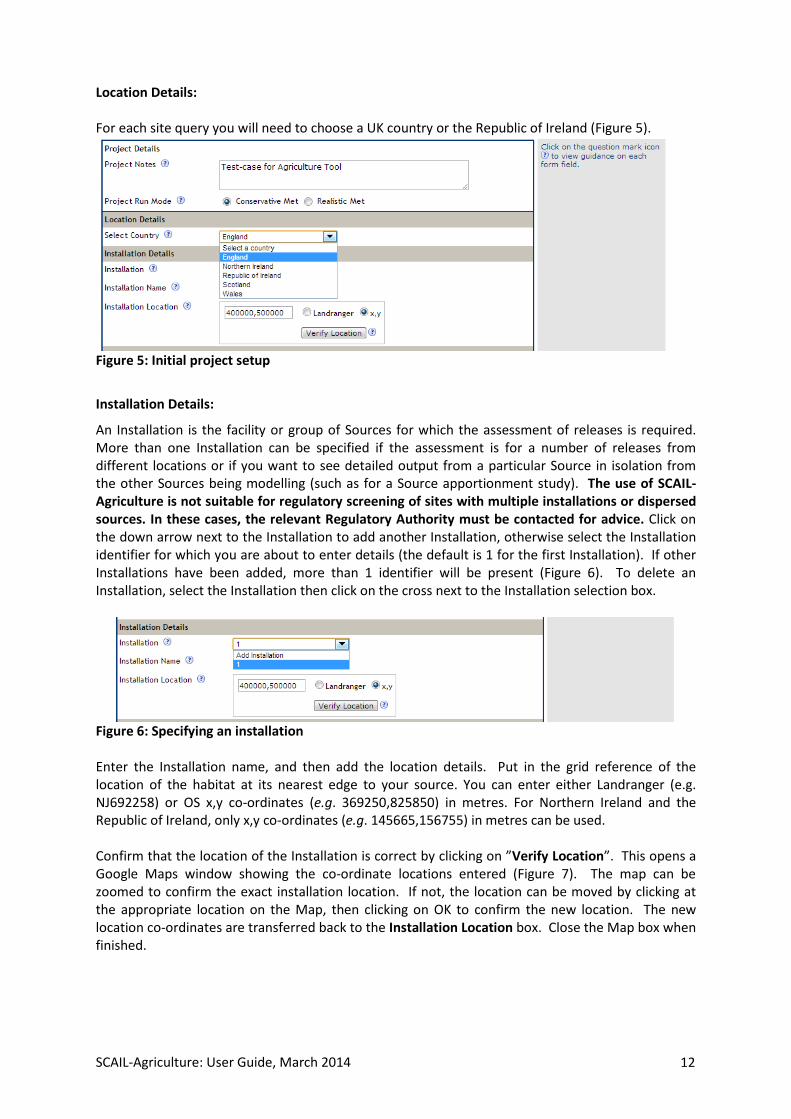
Location Details: For each site query you will need to choose a UK country or the Republic of Ireland (Figure 5).
Figure 5: Initial project setup
Installation Details:
An Installation is the facility or group of Sources for which the assessment of releases is required. More than one Installation can be specified if the assessment is for a number of releases from different locations or if you want to see detailed output from a particular Source in isolation from the other Sources being modelling (such as for a Source apportionment study). The use of SCAIL-Agriculture is not suitable for regulatory screening of sites with multiple installations or dispersed sources. In these cases, the relevant Regulatory Authority must be contacted for advice. Click on the down arrow next to the Installation to add another Installation, otherwise select the Installation identifier for which you are about to enter details (the default is 1 for the first Installation). If other Installations have been added, more than 1 identifier will be present (Figure 6). To delete an Installation, select the Installation then click on the cross next to the Installation selection box.
Figure 6: Specifying an installation Enter the Installation name, and then add the location details. Put in the grid reference of the location of the habitat at its nearest edge to your source. You can enter either Landranger (e.g. NJ692258) or OS x,y co-ordinates (e.g. 369250,825850) in metres. For Northern Ireland and the Republic of Ireland, only x,y co-ordinates (e.g. 145665,156755) in metres can be used. Confirm that the location of the Installation is correct by clicking on ”Verify Location”. This opens a Google Maps window showing the co-ordinate locations entered (Figure 7). The map can be zoomed to confirm the exact installation location. If not, the location can be moved by clicking at the appropriate location on the Map, then clicking on OK to confirm the new location. The new location co-ordinates are transferred back to the Installation Location box. Close the Map box when finished.
SCAIL-Agriculture: User Guide, March 2014 12
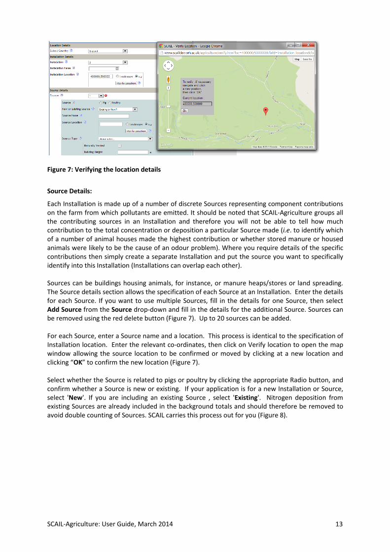
Figure 7: Verifying the location details
Source Details:
Each Installation is made up of a number of discrete Sources representing component contributions on the farm from which pollutants are emitted. It should be noted that SCAIL-Agriculture groups all the contributing sources in an Installation and therefore you will not be able to tell how much contribution to the total concentration or deposition a particular Source made (i.e. to identify which of a number of animal houses made the highest contribution or whether stored manure or housed animals were likely to be the cause of an odour problem). Where you require details of the specific contributions then simply create a separate Installation and put the source you want to specifically identify into this Installation (Installations can overlap each other). Sources can be buildings housing animals, for instance, or manure heaps/stores or land spreading. The Source details section allows the specification of each Source at an Installation. Enter the details for each Source. If you want to use multiple Sources, fill in the details for one Source, then select Add Source from the Source drop-down and fill in the details for the additional Source. Sources can be removed using the red delete button (Figure 7). Up to 20 sources can be added. For each Source, enter a Source name and a location. This process is identical to the specification of Installation location. Enter the relevant co-ordinates, then click on Verify location to open the map window allowing the source location to be confirmed or moved by clicking at a new location and clicking “OK” to confirm the new location (Figure 7). Select whether the Source is related to pigs or poultry by clicking the appropriate Radio button, and confirm whether a Source is new or existing. If your application is for a new Installation or Source, select 'New'. If you are including an existing Source , select 'Existing'. Nitrogen deposition from existing Sources are already included in the background totals and should therefore be removed to avoid double counting of Sources. SCAIL carries this process out for you (Figure 8).
SCAIL-Agriculture: User Guide, March 2014 13

Figure 8: Specifying Source details Select Pig or Poultry depending on the livestock type you are assessing. At this point you are now ready to enter the data that will be used to calculate the emissions coming from the various agricultural Sources. SCAIL uses the same emission factors found in the IPPC application. There are three menus associated with Source type (Figure 8). Most of the time you will need to select all 3. The first select list shows the three main types of agricultural Sources:
1. Housing 2. Litter / Manure Storage 3. Land Spreading
The second select menu will depend on what is selected in the first menu, but it will contain livestock types, storage or land spreading operations. Finally the third select menu gives further detail. The two input boxes are for inputting the number of livestock or area of housing or volume of slurry spread on fields. For example, in Figure 8 the user has selected "Housing", "Layers" and "Ventilated deep pit". There are 10000 layers in the housing unit which has an area of 1000 m2 (50 x
SCAIL-Agriculture: User Guide, March 2014 14

20 m shed). It should be noted that SCAIL-Agriculture includes buildings as cuboids, hence this building will be represented in the tool as having a footprint of 31.6 m x 31.6 m. If housing is selected, you are prompted to specify the building height and select if the building is naturally ventilated. If the building is not naturally ventilated (i.e. it is ventilated by mechanical fans) then specify the location of the ventilation fans as either “Roof” or “Side of Building” using the “Fan Location” drop down. If you do not know the location of the ventilation fans or if there is a roughly even split between fans mounted on the roof and walls of the building then you should select “Side of Building”. When “Roof” mounted fans are selected then you should specify the number of fans, the diameter of a typical exhaust and airflow of a typical fan (Figure 9). If any of information required for including “Roof” mounted fans is unknown then use the “Side of Building” option. Guidelines on the ventilation rates for typical livestock types can be found in Table 2-D of the SCAIL-Agriculture report.
Figure 9: Specifying options for housing Finally specify the Livestock number and the footprint area of the animal housing and the type of animal housed in the building (see Figure 10 for types available). As a guide, the animal welfare regulations (The Welfare of Farmed Animals (England) Regulations 2007) recommends minimum floor areas that must be provided for livestock.
Figure 10: Specifying animal types for housing The last input stage is to specify the housing regime for the animal (Figure 11), then click on the “Get Emission Values” button to populate the values from the database defaults according to the options selected and input values. User-specified values can be added and comments on the Source entered. Where any manual modification is made to the emission rates then suitable comments should be included to provide a record of any assumptions made.
SCAIL-Agriculture: User Guide, March 2014 15
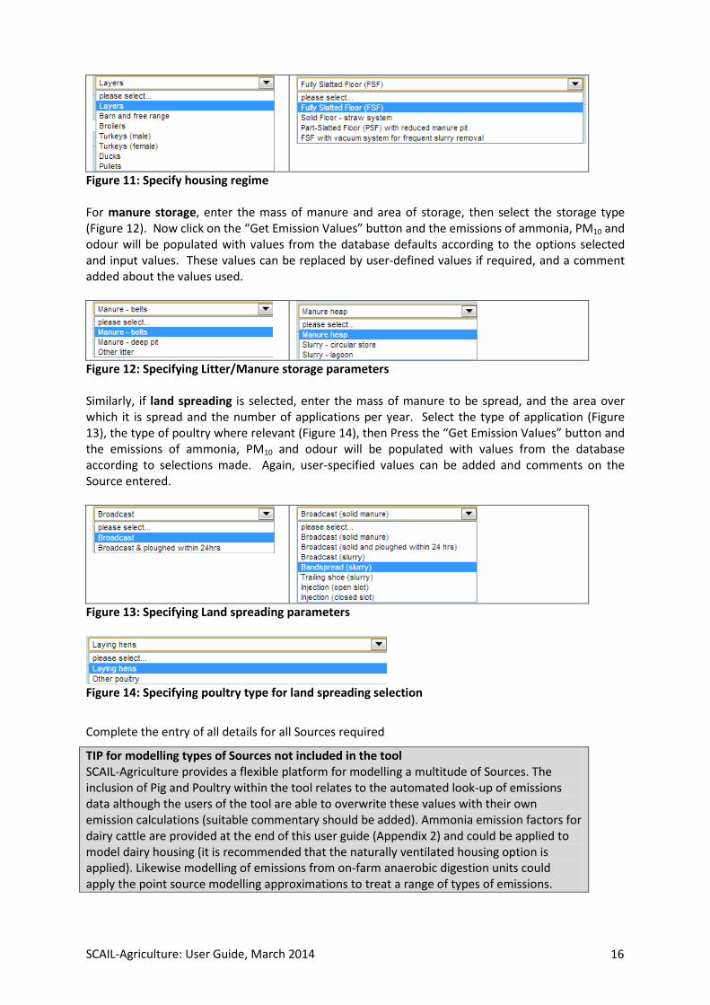
Figure 11: Specify housing regime For manure storage, enter the mass of manure and area of storage, then select the storage type (Figure 12). Now click on the “Get Emission Values” button and the emissions of ammonia, PM10 and odour will be populated with values from the database defaults according to the options selected and input values. These values can be replaced by user-defined values if required, and a comment added about the values used.
Figure 12: Specifying Litter/Manure storage parameters Similarly, if land spreading is selected, enter the mass of manure to be spread, and the area over which it is spread and the number of applications per year. Select the type of application (Figure 13), the type of poultry where relevant (Figure 14), then Press the “Get Emission Values” button and the emissions of ammonia, PM10 and odour will be populated with values from the database according to selections made. Again, user-specified values can be added and comments on the Source entered.
Figure 13: Specifying Land spreading parameters
Figure 14: Specifying poultry type for land spreading selection
Complete the entry of all details for all Sources required
TIP for modelling types of Sources not included in the tool SCAIL-Agriculture provides a flexible platform for modelling a multitude of Sources. The inclusion of Pig and Poultry within the tool relates to the automated look-up of emissions data although the users of the tool are able to overwrite these values with their own emission calculations (suitable commentary should be added). Ammonia emission factors for dairy cattle are provided at the end of this user guide (Appendix 2) and could be applied to model dairy housing (it is recommended that the naturally ventilated housing option is applied). Likewise modelling of emissions from on-farm anaerobic digestion units could apply the point source modelling approximations to treat a range of types of emissions.
SCAIL-Agriculture: User Guide, March 2014 16

Entering designated site details:
Enter the radius over which you would like an automated search of designated sites, then click on the “Run receptor search” button. It should be noted that this search will be centred on the location that was specified for Installation number 1. This searches on-line databases for designated sites within the specified radius from the Installation and produces a list of all sensitive designated sites found (Figure 15). This list shows the site name, the distance to the Installation and the site designation.
Figure 15: Receptor details within a specified distance of an Installation Clicking on the Verify Receptor Locations button produces a map showing the Installation and identified receptor locations (Figure 16). Further information on the specific habits is provided by hovering the mouse over the blue “Receptors” pins; these show the closest edge of the identified habitats. The red “Receptor” pin shows the location of the first Installation that was added.
Figure 16: Confirming Receptor locations in relation to an Installation
SCAIL-Agriculture: User Guide, March 2014 17

There is also the facility to add User-specified sites. This can be used where new sites may have arisen, for example, or where other semi-natural areas need assessing. Click on Add site, then enter a name and location for the site. You should also select the habitat type within the Receptor site (Figure 17).
Figure 17: Specifying habitat type for a user defined receptor Confirm the site location using the map, then at this stage you can use the Check Background Levels button to check the background concentration and deposition levels for each pollutant at the habitat grid reference entered and then compare these levels with the Critical Load/Level of the selected Habitat Type (Figure 18). This information will open in a new window. More User-specified sites can be added in the same way and individual sites can be deleted by selecting the site, then pressing the red delete button next to the Add site button.
Figure 18: Background levels at User-specified habitat sites.
Entering Human Receptor details:
There is also the facility to add User-specified Human Receptor sites. These are used to assess concentrations of PM10 and odour. There are a number of statistics that are relevant for PM10 exposure hence SCAIL Agriculture allows the user to specify either the 90th percentile, 98th percentile or annual average statistic, these are selected using the “PM10 percentile” drop-down shown in Figure 19.
SCAIL-Agriculture: User Guide, March 2014 18

The method is very similar to the addition of user-specified habitat sites as described in the previous section. Click on Add receptor, then enter a name and location for the Receptor. Confirm the site location using the map, then at this stage you can use the Check Background PM10 Levels button to check the background PM10 concentration at the location read from APIS (Figure 19). As before, more Human Receptor sites can be added in the same way and individual receptors can be deleted by selecting the receptor, then pressing the red delete button next to the Add receptor button. It should be noted that background concentrations for odour are not required in the assessment.
Figure 19: Checking PM10 background at specified receptors and selecting the output statistic for PM10 assessments.
Saving the input file:
Use the Save input data button to save all the information entered on the form for this project (Figure 20 and Figure 21). This will enable the same scenario to be run again or modified without having to enter all the information again. A user-specified file can be saved (Figure 20) although this depends on the internet browser that you are using (the options shown in Figure 20 are relevant to Microsoft Internet Explorer). This file should be renamed if you want to save multiple runs in the same folder. If you forget to save the input data at this stage, it can be saved from the results page after the model has run.
Figure 20: Specifying file name for saving input data (options depend on the browser that you are using).
Clearing the Form:
If you want to clear the form, deleting all the Sources that have been set up, click on the Clear Form button (Figure 21). If the input data is required later, make sure you have saved the data first using the Save Input Data button.
SCAIL-Agriculture: User Guide, March 2014 19
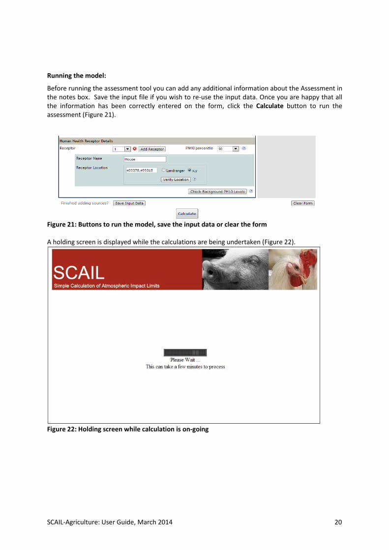
Running the model:
Before running the assessment tool you can add any additional information about the Assessment in the notes box. Save the input file if you wish to re-use the input data. Once you are happy that all the information has been correctly entered on the form, click the Calculate button to run the assessment (Figure 21).
Figure 21: Buttons to run the model, save the input data or clear the form A holding screen is displayed while the calculations are being undertaken (Figure 22).
Figure 22: Holding screen while calculation is on-going
SCAIL-Agriculture: User Guide, March 2014 20
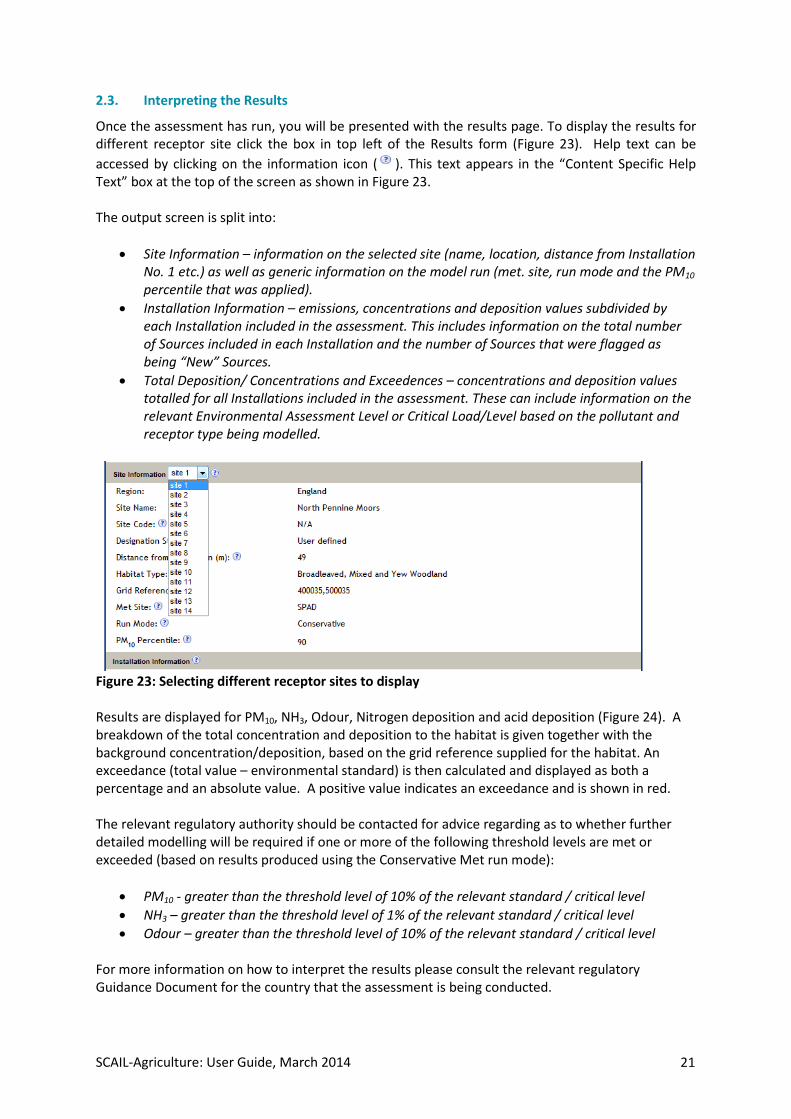
2.3. Interpreting the Results
Once the assessment has run, you will be presented with the results page. To display the results for different receptor site click the box in top left of the Results form (Figure 23). Help text can be accessed by clicking on the information icon ( ). This text appears in the “Content Specific Help Text” box at the top of the screen as shown in Figure 23. The output screen is split into:
• Site Information – information on the selected site (name, location, distance from Installation No. 1 etc.) as well as generic information on the model run (met. site, run mode and the PM10 percentile that was applied).
• Installation Information – emissions, concentrations and deposition values subdivided by each Installation included in the assessment. This includes information on the total number of Sources included in each Installation and the number of Sources that were flagged as being “New” Sources.
• Total Deposition/ Concentrations and Exceedences – concentrations and deposition values totalled for all Installations included in the assessment. These can include information on the relevant Environmental Assessment Level or Critical Load/Level based on the pollutant and receptor type being modelled.
Figure 23: Selecting different receptor sites to display Results are displayed for PM10, NH3, Odour, Nitrogen deposition and acid deposition (Figure 24). A breakdown of the total concentration and deposition to the habitat is given together with the background concentration/deposition, based on the grid reference supplied for the habitat. An exceedance (total value – environmental standard) is then calculated and displayed as both a percentage and an absolute value. A positive value indicates an exceedance and is shown in red. The relevant regulatory authority should be contacted for advice regarding as to whether further detailed modelling will be required if one or more of the following threshold levels are met or exceeded (based on results produced using the Conservative Met run mode):
• PM10 - greater than the threshold level of 10% of the relevant standard / critical level • NH3 – greater than the threshold level of 1% of the relevant standard / critical level • Odour – greater than the threshold level of 10% of the relevant standard / critical level
For more information on how to interpret the results please consult the relevant regulatory Guidance Document for the country that the assessment is being conducted.
SCAIL-Agriculture: User Guide, March 2014 21

Figure 24: Results screen (Displayed Critical Load values are examples only)
SCAIL-Agriculture: User Guide, March 2014 22

Options after running the model:
At the bottom of the results page are several options (Figure 24). The Save Results button will save the output data in CSV (comma separated variables) format, which can be opened in Microsoft Excel. The Save Inputs button can be used to save the input data for this model run if it was not saved on the input form before running the model. You can return to the Input Page by clicking on the Back Page button at the bottom of the page. If you use your browser’s Back button to go back to the input page, you may lose the input data you filled out on the form.
SCAIL-Agriculture: User Guide, March 2014 23

Appendix 1: Typical Meteorological Year Wind Roses
Table A1.1: Details of meteorological sites included in SCAIL-Agriculture
Station Name (Short)
Station Grid
Station X Coordinate (m)
Station Y Coordinate (m)
Station Elevation (m)
Wind Direction (degrees)
AVIEMORE AVIE OS 289652 814315 228 210 BALLYKELLY BALL IRL 263400 423800 4 110 BOULMER BOUL OS 425300 614200 23 250 CARDIFF WEATHER CENTRE CARD OS 318200 176100 52 230
CHURCH FENTON CHUR OS 452818 438027 8 270 COLESHILL COLE OS 421090 286940 96 200 CROSBY CROS OS 329940 400570 9 150 EDINBURGH GOGARBANK EDIN OS 316100 671400 57 250 ESKDALEMUIR ESKD OS 323500 602600 242 190 GLASGOW BISHOPTON GLAS OS 241788 671073 59 210 HEATHROW HEAT OS 507700 176700 25 210 ISLAY PORT ELLEN ISLA OS 132900 651300 17 140 ISLE OF PORTLAND ISLE OS 367798 69251 52 250 LERWICK LERW OS 445392 1139664 82 170 LEUCHARS LEUC OS 346800 720900 10 260 LOSSIEMOUTH LOSS OS 321249 869822 6 250 LYNEHAM LYNE OS 400629 178255 145 210 MARHAM MARH OS 573700 309100 21 210 MUMBLES HEAD MUMB OS 262700 187000 32 270 PLYMOUTH MOUNTBATTEN PLYM OS 249219 52714 50 90
PORTGLENONE PORT IRL 299100 403100 64 330 SENNYBRIDGE NO 2 SENN OS 289408 241777 307 230 SKYE LUSA SKYE OS 170593 824888 18 210 SPADEADAM NO 2 SPAD OS 364700 573000 285 250 STORNOWAY AIRPORT STOR OS 146443 933104 15 190 VALLEY VALL OS 230885 375849 10 210 DYCE DYCE OS 387810 812800 62 170 PRESTWICK RNAS PRES OS 236902 627653 10 250 TIREE TIRE OS 99900 744600 10 190 WICK AIRPORT WICK OS 336490 952230 30 150 BELLMULLET BELL IRL 70220 335187 11 190 BIRR BIRR IRL 206158 205628 73 190 CASEMENT CASE IRL 303878 229925 94 220 CORK CORK IRL 166139 65739 154 220 DUBLIN AIRPORT DUBL IRL 316878 243079 71 250 KILLKENNY KILK IRL 250828 155810 66 180 KNOCK KNOC IRL 139548 282924 205 210 MULLINGAR MULL IRL 243023 253295 104 220 ROSSLARE ROSS IRL 309980 114606 26 220 SHANNON SHAN IRL 138530 162095 6 250 VALENTIA VALE IRL 45204 77945 25 170
SCAIL-Agriculture: User Guide, March 2014 24
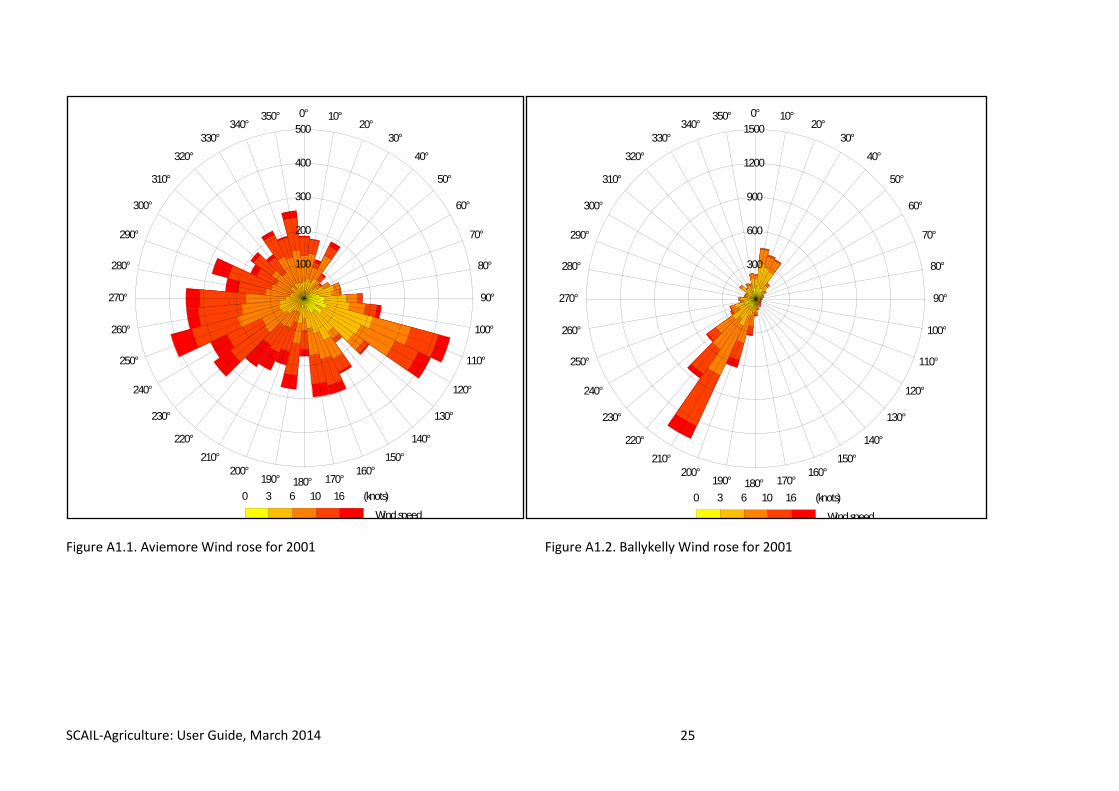
Figure A1.1. Aviemore Wind rose for 2001 Figure A1.2. Ballykelly Wind rose for 2001
0 3 6 10 16 (knots)
Wind speed
0° 10°20°
30°40°
50°
60°
70°
80°
90°
100°
110°
120°
130°
140°150°
160°170°180°190°
200°210°
220°
230°
240°
250°
260°
270°
280°
290°
300°
310°
320°330°
340°350°
100
200
300
400
500
0 3 6 10 16 (knots)
Wind speed
0° 10°20°
30°40°
50°
60°
70°
80°
90°
100°
110°
120°
130°
140°150°
160°170°180°190°
200°210°
220°
230°
240°
250°
260°
270°
280°
290°
300°
310°
320°330°
340°350°
300
600
900
1200
1500
SCAIL-Agriculture: User Guide, March 2014 25

Figure A1.3. Boulmer Wind rose for 2004 Figure A1.4. Cardiff Weather Centre Wind rose for 2003
0 3 6 10 16 (knots)
Wind speed
0° 10°20°
30°40°
50°
60°
70°
80°
90°
100°
110°
120°
130°
140°150°
160°170°180°190°
200°210°
220°
230°
240°
250°
260°
270°
280°
290°
300°
310°
320°330°
340°350°
200
400
600
800
0 3 6 10 16 (knots)
Wind speed
0° 10°20°
30°40°
50°
60°
70°
80°
90°
100°
110°
120°
130°
140°150°
160°170°180°190°
200°210°
220°
230°
240°
250°
260°
270°
280°
290°
300°
310°
320°330°
340°350°
200
400
600
800
1000
SCAIL-Agriculture: User Guide, March 2014 26

Figure A1.5. Church Fenton Wind rose 2003 Figure A1.6. Coleshill Wind rose for 2001
0 3 6 10 16 (knots)
Wind speed
0° 10°20°
30°40°
50°
60°
70°
80°
90°
100°
110°
120°
130°
140°150°
160°170°180°190°
200°210°
220°
230°
240°
250°
260°
270°
280°
290°
300°
310°
320°330°
340°350°
100
200
300
400
500
0 3 6 10 16 (knots)
Wind speed
0° 10°20°
30°40°
50°
60°
70°
80°
90°
100°
110°
120°
130°
140°150°
160°170°180°190°
200°210°
220°
230°
240°
250°
260°
270°
280°
290°
300°
310°
320°330°
340°350°
100
200
300
400
500
SCAIL-Agriculture: User Guide, March 2014 27

Figure A1.7. Crosby Wind rose for 2001 Figure A1.8. Edinburgh Gogarbank Wind rose for 2003
0 3 6 10 16 (knots)
Wind speed
0° 10°20°
30°40°
50°
60°
70°
80°
90°
100°
110°
120°
130°
140°150°
160°170°180°190°
200°210°
220°
230°
240°
250°
260°
270°
280°
290°
300°
310°
320°330°
340°350°
100
200
300
400
500
600
0 3 6 10 16 (knots)
Wind speed
0° 10°20°
30°40°
50°
60°
70°
80°
90°
100°
110°
120°
130°
140°150°
160°170°180°190°
200°210°
220°
230°
240°
250°
260°
270°
280°
290°
300°
310°
320°330°
340°350°
200
400
600
800
1000
SCAIL-Agriculture: User Guide, March 2014 28
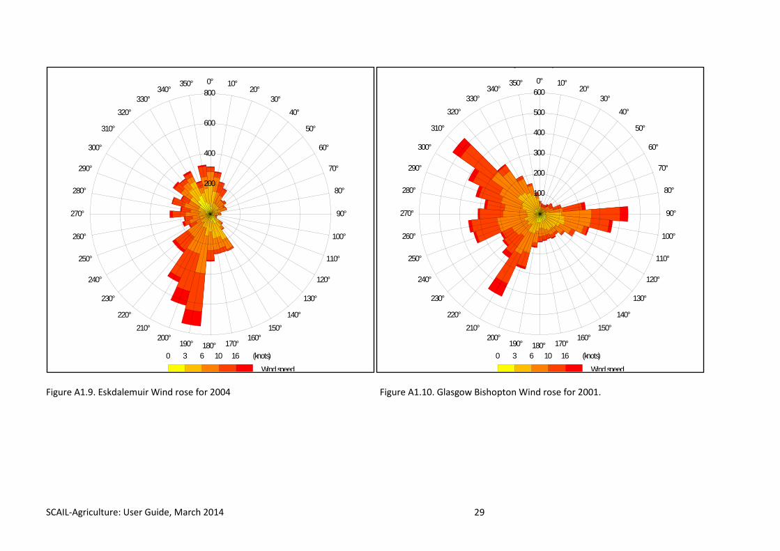
Figure A1.9. Eskdalemuir Wind rose for 2004 Figure A1.10. Glasgow Bishopton Wind rose for 2001.
0 3 6 10 16 (knots)
Wind speed
0° 10°20°
30°40°
50°
60°
70°
80°
90°
100°
110°
120°
130°
140°150°
160°170°180°190°
200°210°
220°
230°
240°
250°
260°
270°
280°
290°
300°
310°
320°330°
340°350°
200
400
600
800
g p
0 3 6 10 16 (knots)
Wind speed
0° 10°20°
30°40°
50°
60°
70°
80°
90°
100°
110°
120°
130°
140°150°
160°170°180°190°
200°210°
220°
230°
240°
250°
260°
270°
280°
290°
300°
310°
320°330°
340°350°
100
200
300
400
500
600
SCAIL-Agriculture: User Guide, March 2014 29

Figure A1.11. Heathrow Wind rose for 2001 Figure A1.12. Islay Port Ellen wind rose for 2005
0 3 6 10 16 (knots)
Wind speed
0° 10°20°
30°40°
50°
60°
70°
80°
90°
100°
110°
120°
130°
140°150°
160°170°180°190°
200°210°
220°
230°
240°
250°
260°
270°
280°
290°
300°
310°
320°330°
340°350°
100
200
300
400
500
600
y
0 3 6 10 16 (knots)
Wind speed
0° 10°20°
30°40°
50°
60°
70°
80°
90°
100°
110°
120°
130°
140°150°
160°170°180°190°
200°210°
220°
230°
240°
250°
260°
270°
280°
290°
300°
310°
320°330°
340°350°
100
200
300
400
500
SCAIL-Agriculture: User Guide, March 2014 30
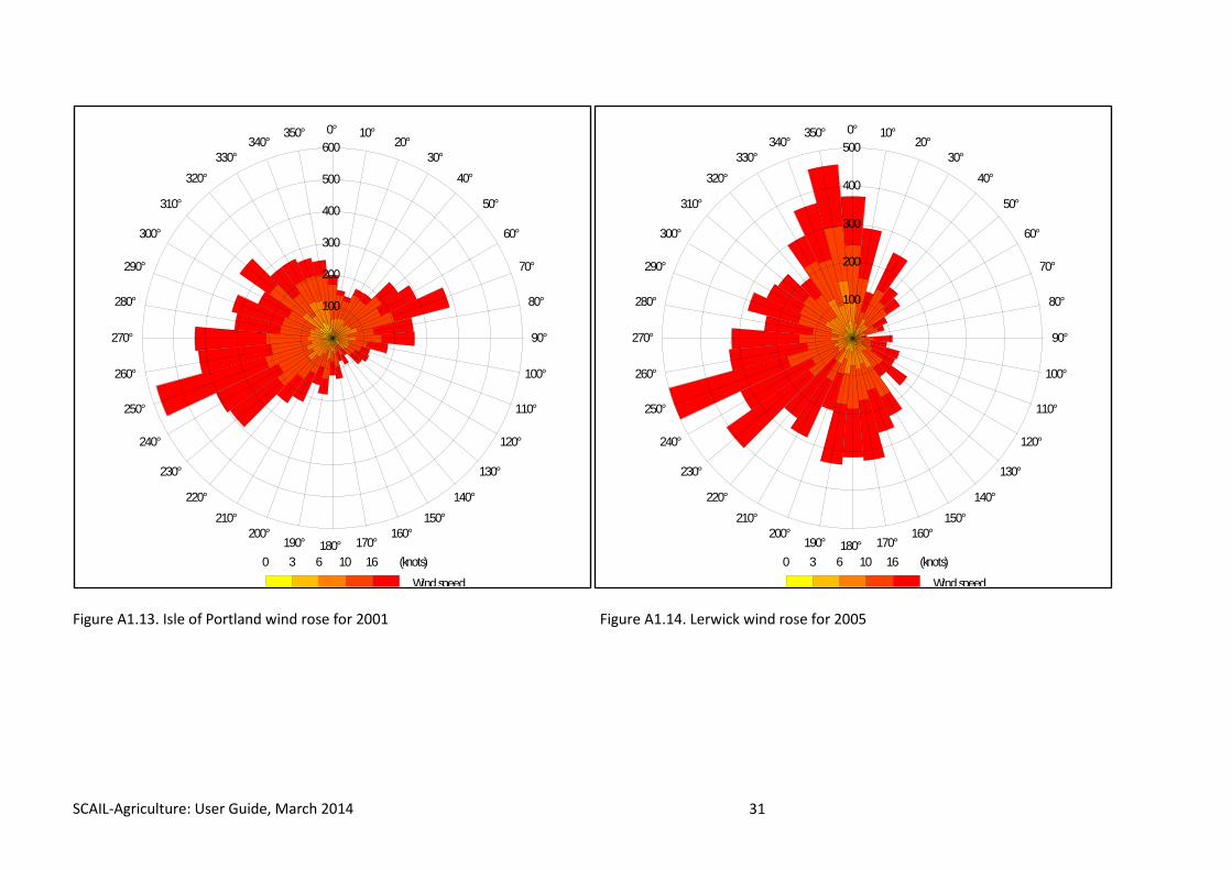
Figure A1.13. Isle of Portland wind rose for 2001 Figure A1.14. Lerwick wind rose for 2005
0 3 6 10 16 (knots)
Wind speed
0° 10°20°
30°40°
50°
60°
70°
80°
90°
100°
110°
120°
130°
140°150°
160°170°180°190°
200°210°
220°
230°
240°
250°
260°
270°
280°
290°
300°
310°
320°330°
340°350°
100
200
300
400
500
600
0 3 6 10 16 (knots)
Wind speed
0° 10°20°
30°40°
50°
60°
70°
80°
90°
100°
110°
120°
130°
140°150°
160°170°180°190°
200°210°
220°
230°
240°
250°
260°
270°
280°
290°
300°
310°
320°330°
340°350°
100
200
300
400
500
SCAIL-Agriculture: User Guide, March 2014 31

Figure A1.15. Leuchars wind rose 2003 Figure A1.16. Lossiemouth wind rose 2004
0 3 6 10 16 (knots)
Wind speed
0° 10°20°
30°40°
50°
60°
70°
80°
90°
100°
110°
120°
130°
140°150°
160°170°180°190°
200°210°
220°
230°
240°
250°
260°
270°
280°
290°
300°
310°
320°330°
340°350°
200
400
600
800
1000
0 3 6 10 16 (knots)
Wind speed
0° 10°20°
30°40°
50°
60°
70°
80°
90°
100°
110°
120°
130°
140°150°
160°170°180°190°
200°210°
220°
230°
240°
250°
260°
270°
280°
290°
300°
310°
320°330°
340°350°
200
400
600
800
SCAIL-Agriculture: User Guide, March 2014 32

Figure A1.17. Lyneham wind rose for 2002 Figure A1.18. Marham wind rose for 2001
y
0 3 6 10 16 (knots)
Wind speed
0° 10°20°
30°40°
50°
60°
70°
80°
90°
100°
110°
120°
130°
140°150°
160°170°180°190°
200°210°
220°
230°
240°
250°
260°
270°
280°
290°
300°
310°
320°330°
340°350°
100
200
300
400
500
600
0 3 6 10 16 (knots)
Wind speed
0° 10°20°
30°40°
50°
60°
70°
80°
90°
100°
110°
120°
130°
140°150°
160°170°180°190°
200°210°
220°
230°
240°
250°
260°
270°
280°
290°
300°
310°
320°330°
340°350°
100
200
300
400
500
SCAIL-Agriculture: User Guide, March 2014 33
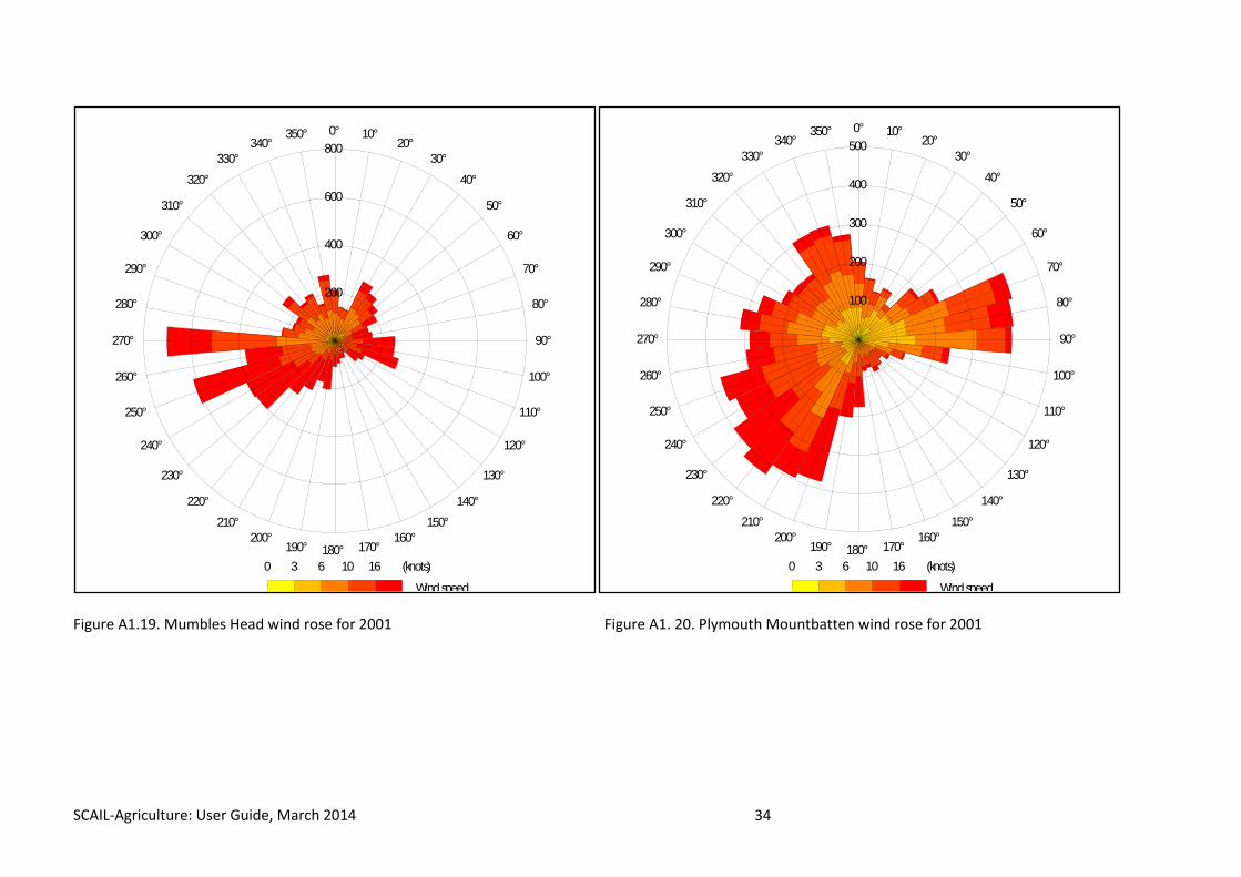
Figure A1.19. Mumbles Head wind rose for 2001 Figure A1. 20. Plymouth Mountbatten wind rose for 2001
0 3 6 10 16 (knots)
Wind speed
0° 10°20°
30°40°
50°
60°
70°
80°
90°
100°
110°
120°
130°
140°150°
160°170°180°190°
200°210°
220°
230°
240°
250°
260°
270°
280°
290°
300°
310°
320°330°
340°350°
200
400
600
800
0 3 6 10 16 (knots)
Wind speed
0° 10°20°
30°40°
50°
60°
70°
80°
90°
100°
110°
120°
130°
140°150°
160°170°180°190°
200°210°
220°
230°
240°
250°
260°
270°
280°
290°
300°
310°
320°330°
340°350°
100
200
300
400
500
SCAIL-Agriculture: User Guide, March 2014 34
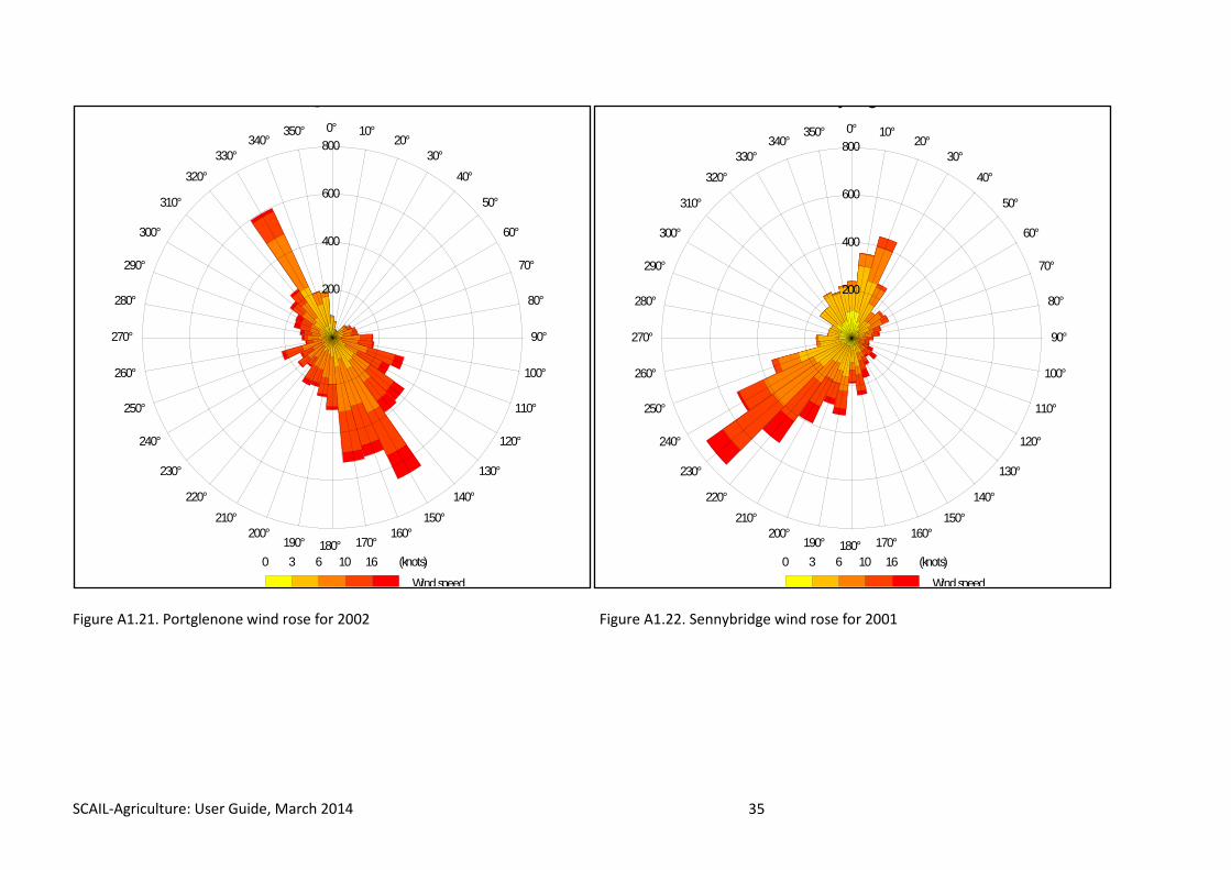
Figure A1.21. Portglenone wind rose for 2002 Figure A1.22. Sennybridge wind rose for 2001
g
0 3 6 10 16 (knots)
Wind speed
0° 10°20°
30°40°
50°
60°
70°
80°
90°
100°
110°
120°
130°
140°150°
160°170°180°190°
200°210°
220°
230°
240°
250°
260°
270°
280°
290°
300°
310°
320°330°
340°350°
200
400
600
800
y g
0 3 6 10 16 (knots)
Wind speed
0° 10°20°
30°40°
50°
60°
70°
80°
90°
100°
110°
120°
130°
140°150°
160°170°180°190°
200°210°
220°
230°
240°
250°
260°
270°
280°
290°
300°
310°
320°330°
340°350°
200
400
600
800
SCAIL-Agriculture: User Guide, March 2014 35

Figure A1.23. Skye Lusa wind rose for 2004 Figure A1.24. Spadeadam wind rose for 2001
y
0 3 6 10 16 (knots)
Wind speed
0° 10°20°
30°40°
50°
60°
70°
80°
90°
100°
110°
120°
130°
140°150°
160°170°180°190°
200°210°
220°
230°
240°
250°
260°
270°
280°
290°
300°
310°
320°330°
340°350°
200
400
600
800
1000
0 3 6 10 16 (knots)
Wind speed
0° 10°20°
30°40°
50°
60°
70°
80°
90°
100°
110°
120°
130°
140°150°
160°170°180°190°
200°210°
220°
230°
240°
250°
260°
270°
280°
290°
300°
310°
320°330°
340°350°
300
600
900
1200
SCAIL-Agriculture: User Guide, March 2014 36
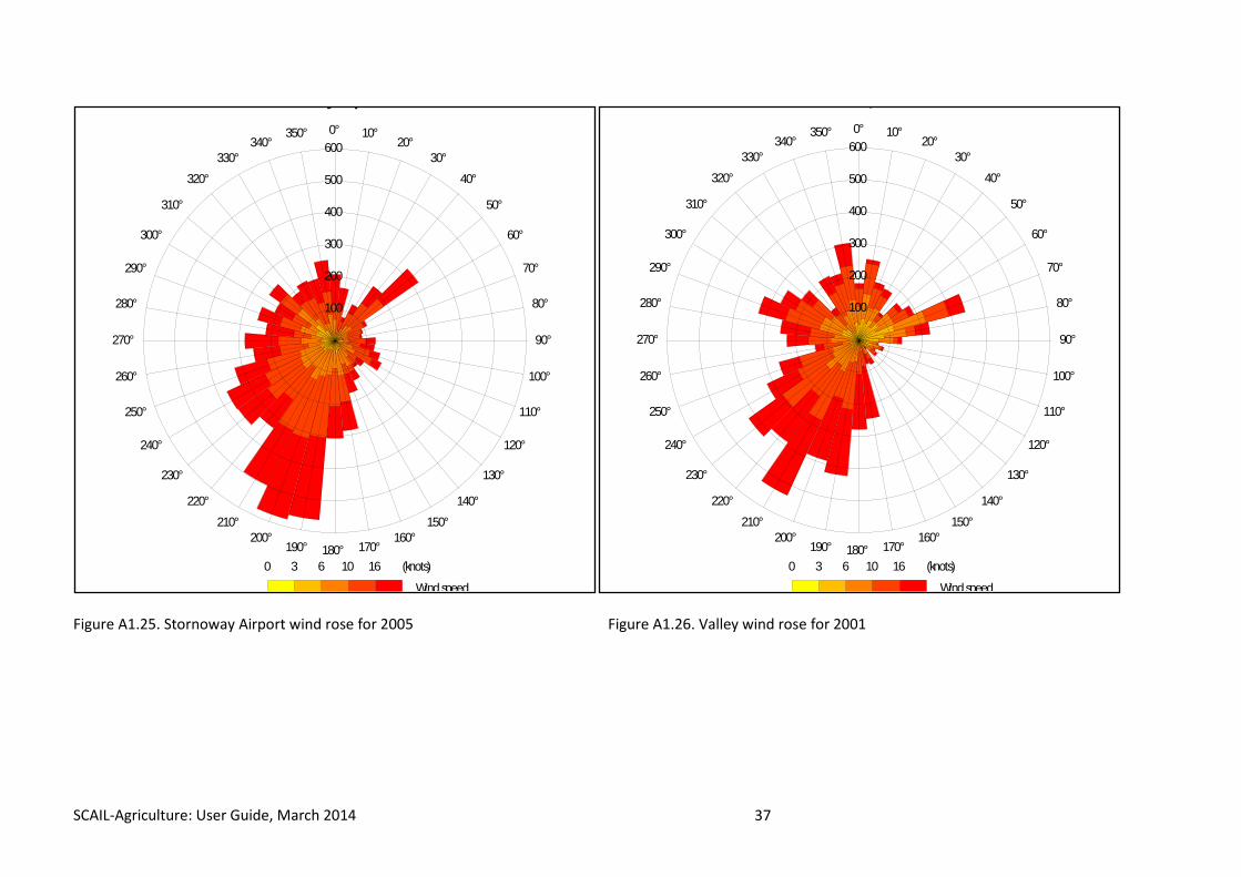
Figure A1.25. Stornoway Airport wind rose for 2005 Figure A1.26. Valley wind rose for 2001
y p
0 3 6 10 16 (knots)
Wind speed
0° 10°20°
30°40°
50°
60°
70°
80°
90°
100°
110°
120°
130°
140°150°
160°170°180°190°
200°210°
220°
230°
240°
250°
260°
270°
280°
290°
300°
310°
320°330°
340°350°
100
200
300
400
500
600
y
0 3 6 10 16 (knots)
Wind speed
0° 10°20°
30°40°
50°
60°
70°
80°
90°
100°
110°
120°
130°
140°150°
160°170°180°190°
200°210°
220°
230°
240°
250°
260°
270°
280°
290°
300°
310°
320°330°
340°350°
100
200
300
400
500
600
SCAIL-Agriculture: User Guide, March 2014 37
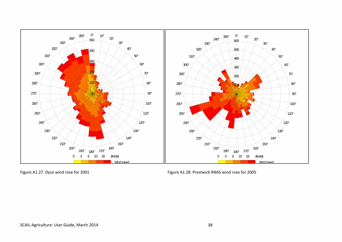
Figure A1.27. Dyce wind rose for 2001 Figure A1.28. Prestwick RNAS wind rose for 2005
0 3 6 10 16 (knots)
Wind speed
0° 10°20°
30°40°
50°
60°
70°
80°
90°
100°
110°
120°
130°
140°150°
160°170°180°190°
200°210°
220°
230°
240°
250°
260°
270°
280°
290°
300°
310°
320°330°
340°350°
100
200
300
400
500
0 3 6 10 16 (knots)
Wind speed
0° 10°20°
30°40°
50°
60°
70°
80°
90°
100°
110°
120°
130°
140°150°
160°170°180°190°
200°210°
220°
230°
240°
250°
260°
270°
280°
290°
300°
310°
320°330°
340°350°
100
200
300
400
500
600
SCAIL-Agriculture: User Guide, March 2014 38

Figure A1.29. Tiree wind rose for 2005 Figure A1.30. Wick Airport wind rose for 2001
0 3 6 10 16 (knots)
Wind speed
0° 10°20°
30°40°
50°
60°
70°
80°
90°
100°
110°
120°
130°
140°150°
160°170°180°190°
200°210°
220°
230°
240°
250°
260°
270°
280°
290°
300°
310°
320°330°
340°350°
100
200
300
400
500
p
0 3 6 10 16 (knots)
Wind speed
0° 10°20°
30°40°
50°
60°
70°
80°
90°
100°
110°
120°
130°
140°150°
160°170°180°190°
200°210°
220°
230°
240°
250°
260°
270°
280°
290°
300°
310°
320°330°
340°350°
100
200
300
400
500
SCAIL-Agriculture: User Guide, March 2014 39

Figure A1.31. Belmullet wind rose for 2002 Figure A1.32. Birr wind rose for 2005
0
0
3
1.5
6
3.1
10
5.1
16
8.2
(knots)
(m/s)
Wind speed
0° 10°20°
30°40°
50°
60°
70°
80°
90°
100°
110°
120°
130°
140°150°
160°170°180°190°
200°210°
220°
230°
240°
250°
260°
270°
280°
290°
300°
310°
320°330°
340°350°
100
200
300
400
500
0
0
3
1.5
6
3.1
10
5.1
16
8.2
(knots)
(m/s)
Wind speed
0° 10°20°
30°40°
50°
60°
70°
80°
90°
100°
110°
120°
130°
140°150°
160°170°180°190°
200°210°
220°
230°
240°
250°
260°
270°
280°
290°
300°
310°
320°330°
340°350°
100
200
300
400
500
SCAIL-Agriculture: User Guide, March 2014 40
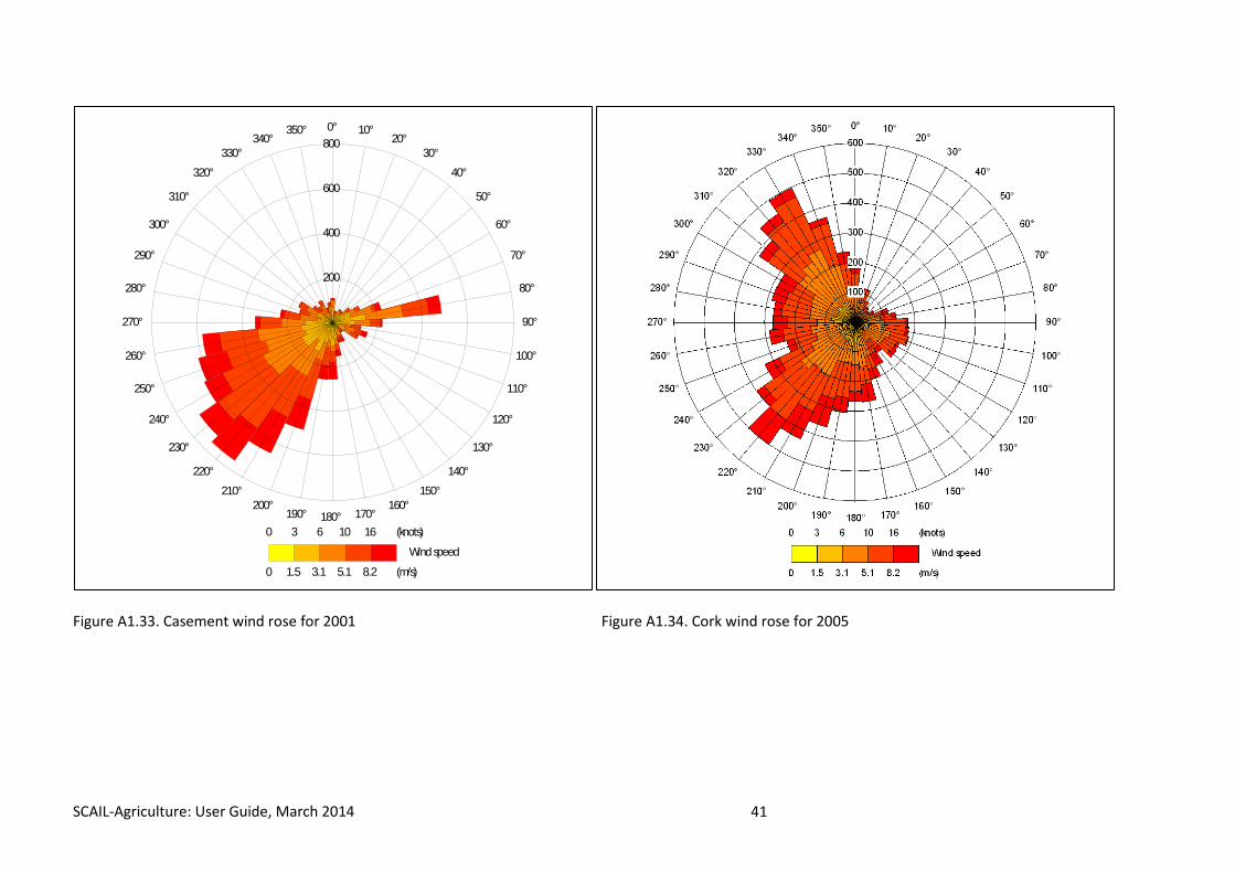
Figure A1.33. Casement wind rose for 2001 Figure A1.34. Cork wind rose for 2005
_ _
0
0
3
1.5
6
3.1
10
5.1
16
8.2
(knots)
(m/s)
Wind speed
0° 10°20°
30°40°
50°
60°
70°
80°
90°
100°
110°
120°
130°
140°150°
160°170°180°190°
200°210°
220°
230°
240°
250°
260°
270°
280°
290°
300°
310°
320°330°
340°350°
200
400
600
800
SCAIL-Agriculture: User Guide, March 2014 41
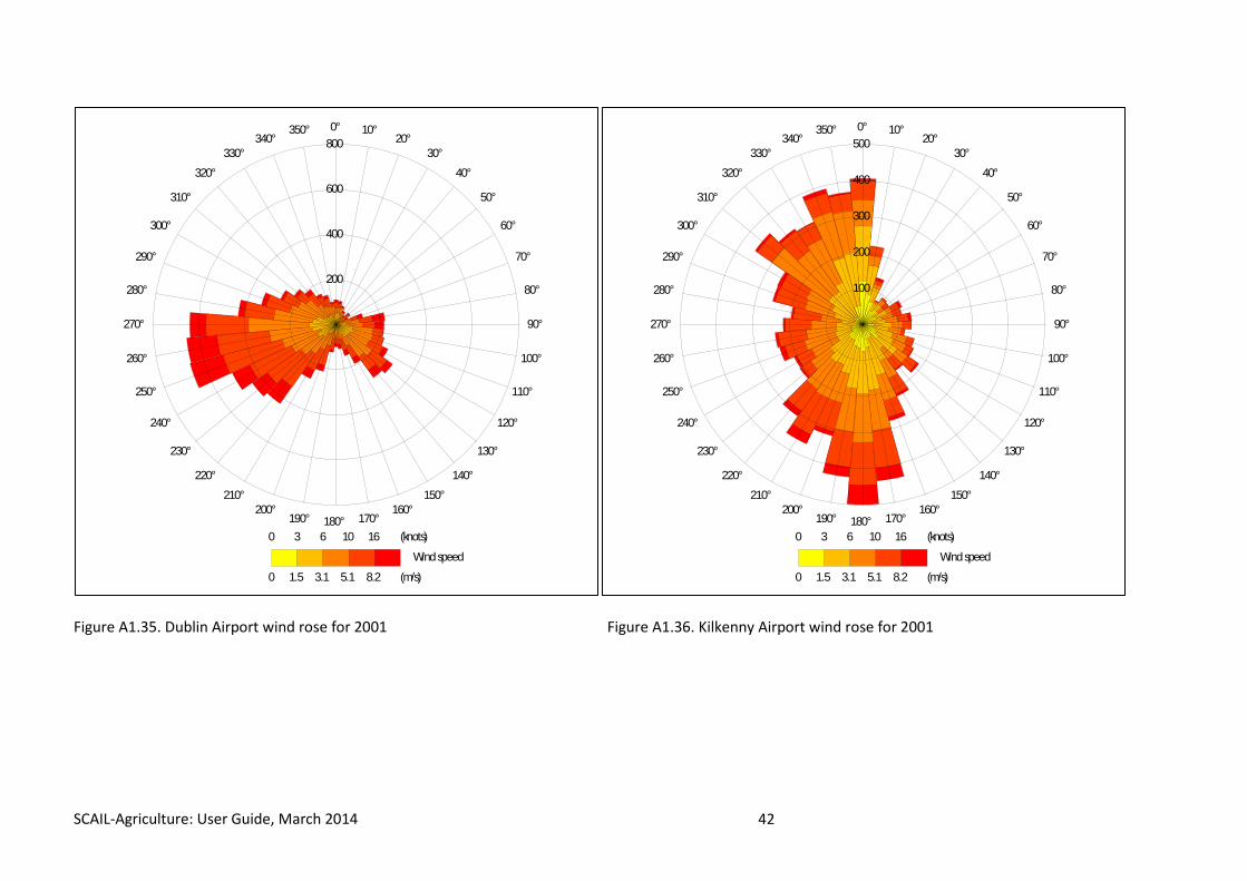
Figure A1.35. Dublin Airport wind rose for 2001 Figure A1.36. Kilkenny Airport wind rose for 2001
0
0
3
1.5
6
3.1
10
5.1
16
8.2
(knots)
(m/s)
Wind speed
0° 10°20°
30°40°
50°
60°
70°
80°
90°
100°
110°
120°
130°
140°150°
160°170°180°190°
200°210°
220°
230°
240°
250°
260°
270°
280°
290°
300°
310°
320°330°
340°350°
200
400
600
800
0
0
3
1.5
6
3.1
10
5.1
16
8.2
(knots)
(m/s)
Wind speed
0° 10°20°
30°40°
50°
60°
70°
80°
90°
100°
110°
120°
130°
140°150°
160°170°180°190°
200°210°
220°
230°
240°
250°
260°
270°
280°
290°
300°
310°
320°330°
340°350°
100
200
300
400
500
SCAIL-Agriculture: User Guide, March 2014 42

Figure A1.37. Knock wind rose for 2005 Figure A1.38. Mullingar wind rose for 2005
_ _
0
0
3
1.5
6
3.1
10
5.1
16
8.2
(knots)
(m/s)
Wind speed
0° 10°20°
30°40°
50°
60°
70°
80°
90°
100°
110°
120°
130°
140°150°
160°170°180°190°
200°210°
220°
230°
240°
250°
260°
270°
280°
290°
300°
310°
320°330°
340°350°
100
200
300
400
500
600
g
0
0
3
1.5
6
3.1
10
5.1
16
8.2
(knots)
(m/s)
Wind speed
0° 10°20°
30°40°
50°
60°
70°
80°
90°
100°
110°
120°
130°
140°150°
160°170°180°190°
200°210°
220°
230°
240°
250°
260°
270°
280°
290°
300°
310°
320°330°
340°350°
100
200
300
400
500
600
SCAIL-Agriculture: User Guide, March 2014 43
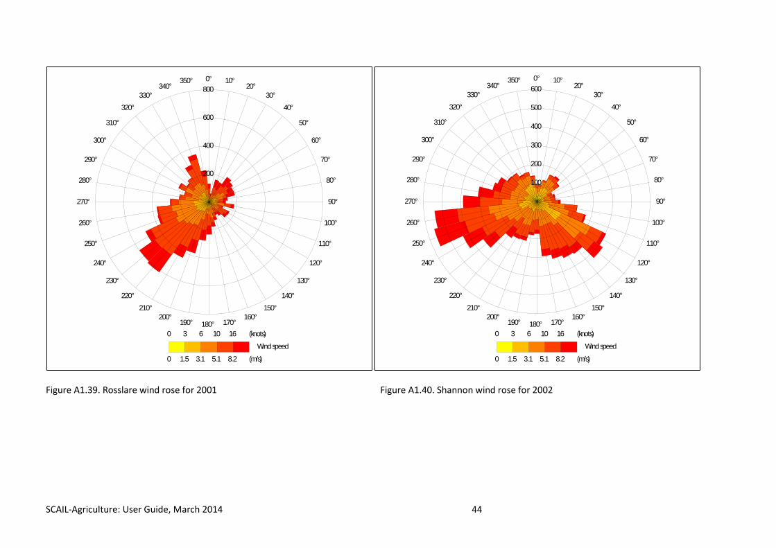
Figure A1.39. Rosslare wind rose for 2001 Figure A1.40. Shannon wind rose for 2002
0
0
3
1.5
6
3.1
10
5.1
16
8.2
(knots)
(m/s)
Wind speed
0° 10°20°
30°40°
50°
60°
70°
80°
90°
100°
110°
120°
130°
140°150°
160°170°180°190°
200°210°
220°
230°
240°
250°
260°
270°
280°
290°
300°
310°
320°330°
340°350°
200
400
600
800
0
0
3
1.5
6
3.1
10
5.1
16
8.2
(knots)
(m/s)
Wind speed
0° 10°20°
30°40°
50°
60°
70°
80°
90°
100°
110°
120°
130°
140°150°
160°170°180°190°
200°210°
220°
230°
240°
250°
260°
270°
280°
290°
300°
310°
320°330°
340°350°
100
200
300
400
500
600
SCAIL-Agriculture: User Guide, March 2014 44
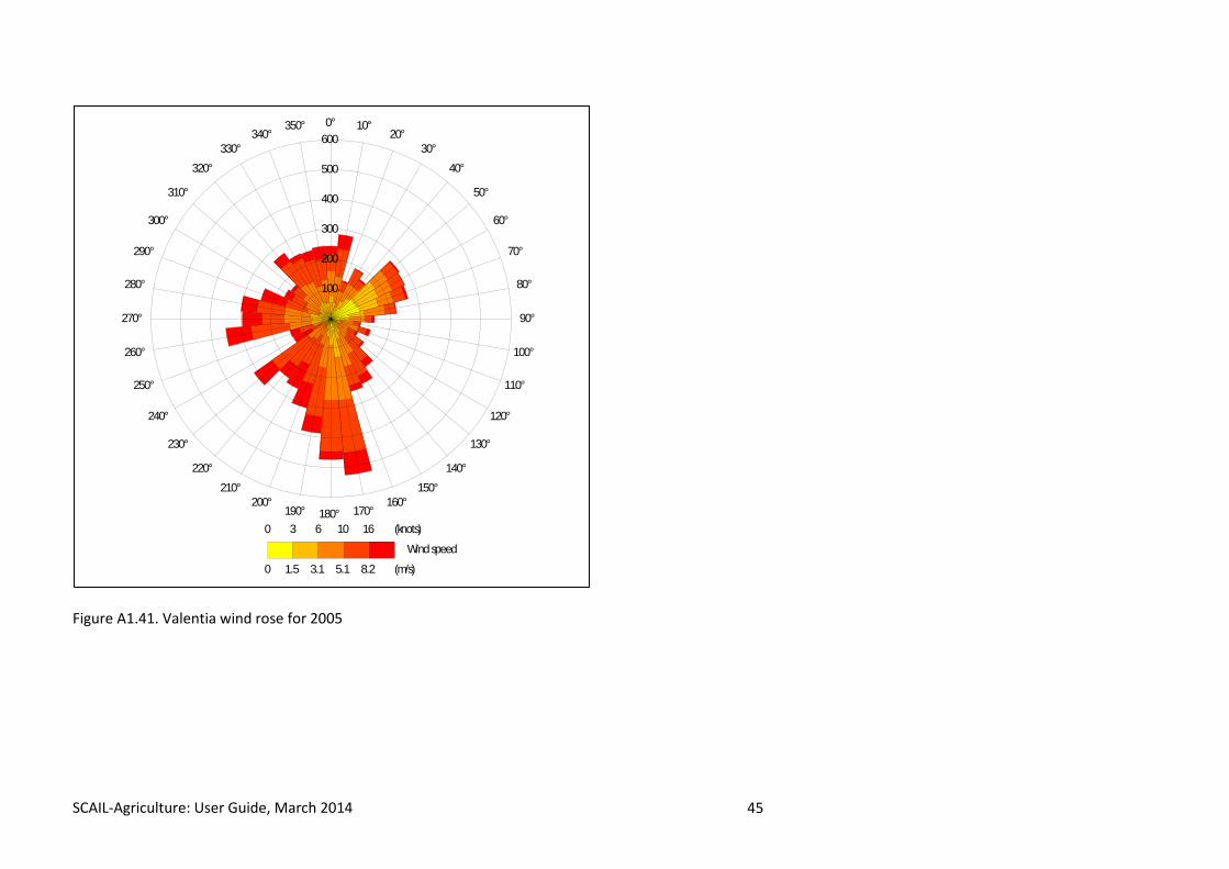
Figure A1.41. Valentia wind rose for 2005
0
0
3
1.5
6
3.1
10
5.1
16
8.2
(knots)
(m/s)
Wind speed
0° 10°20°
30°40°
50°
60°
70°
80°
90°
100°
110°
120°
130°
140°150°
160°170°180°190°
200°210°
220°
230°
240°
250°
260°
270°
280°
290°
300°
310°
320°330°
340°350°
100
200
300
400
500
600
SCAIL-Agriculture: User Guide, March 2014 45

Appendix 2: Ammonia Emission Factors for Cattle
Livestock category Housing emission
Storage emission
Spreading emission
Grazing/outdoor emission
Dairy cows & heifers 1.70E+01 5.15E+00 9.28E+00 2.01E+00 Dairy heifers in calf 5.04E+00 1.57E+00 2.24E+00 1.89E+00 Dairy replacements 4.21E+00 1.31E+00 1.87E+00 1.58E+00 Dairy calves 9.51E-01 1.66E+00 1.83E+00 9.10E-01 Beef cows & heifers 6.45E+00 1.87E+00 2.69E+00 2.14E+00 Beef heifers in calf 4.57E+00 1.33E+00 1.91E+00 1.52E+00 Beef >1yr 4.57E+00 1.33E+00 1.91E+00 1.52E+00 Beef calves 9.51E-01 1.65E+00 1.84E+00 9.10E-01
Emissions are quoted in Kg NH3 per animal per year.
SCAIL-Agriculture: User Guide, March 2014 46

© Sniffer 2014 All rights reserved. No part of this document may be reproduced, stored in a retrieval system or transmitted, in any form or by any means, electronic, mechanical, photocopying, recording or otherwise without the prior permission of Sniffer. The views expressed in this document are not necessarily those of Sniffer. Its members, servants or agents accept no liability whatsoever for any loss or damage arising from the interpretation or use of the information, or reliance upon views contained herein. Dissemination status Unrestricted Project funders Environment Agency Scottish Environment Protection Agency Northern Ireland Environment Agency Whilst this document is considered to represent the best available scientific information and expert opinion available at the stage of completion of the report, it does not necessarily represent the final or policy positions of the project funders. Research contractor This document was produced by: Jacobs UK Ltd, 1080 Eskdale Road. Winnersh, Wokingham, RG41 5TU Centre for Ecology & Hydrology Maclean Building Benson Lane Crowmarsh Gifford Wallingford Oxfordshire OX10 8BB
Sniffer’s project manager Sniffer’s project manager for this contract is: Michelagh O'Neill, Sniffer Sniffer’s technical advisory group is: Rob Kinnersley, Environment Agency – Principal technical advisor Alan McDonald, Scottish Environment Protection Agency Alison Long, Scottish Environment Protection Agency Åsa Hedmark, Scottish Environment Protection Agency John McEntagart, Environmental Protection Agency Ciara Maxwell, Environmental Protection Agency David Bruce, Northern Ireland Environment Agency Clare Whitfield, Joint Nature Conservation Committee Simon Bareham, Natural Resources Wales Ji Ping Shi, Natural Resources Wales
Sniffer is a charity delivering knowledge-based solutions to resilience and sustainability issues. We create and use breakthrough ideas and collaborative approaches across sectors, to make Scotland a more resilient place to live, work and play. Through innovative partnership approaches we share good practice, synthesise and translate evidence, commission new studies and target communications, guidance and training. Sniffer is a company limited by guarantee and a registered charity with offices in Edinburgh.
Sniffer, Greenside House, 25 Greenside Place, Edinburgh, EH1 3AA, Scotland, UK
T: 0131 557 2140 E: [email protected] W: ww.sniffer.org.uk Scotland & Northern Ireland Forum for Environmental Research (Sniffer), Scottish Charity No SC022375, Company No SC149513. Registered in Edinburgh. Registered Office: Edinburgh Quay, 133 Fountainbridge, Edinburgh, EH3 9AG
SCAIL-Agriculture: User Guide, March 2014 47