Scalable and Interactive Segmentation and Visualization

of Neural Processes in EM Datasets

Won-Ki Jeong, Johanna Beyer, Student Member, IEEE,

Markus Hadwiger, Member, IEEE, Amelio Vazquez, Student Member, IEEE,

Hanspeter Pfister, Senior Member, IEEE, and Ross T. Whitaker, Member, IEEE

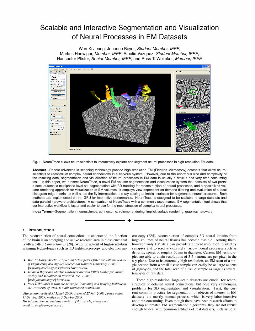
Fig. 1. NeuroTrace allows neuroscientists to interactively explore and segment neural processes in high-resolution EM data.

Abstract—Recent advances in scanning technology provide high resolution EM (Electron Microscopy) datasets that allow neuro-scientists to reconstruct complex neural connections in a nervous system. However, due to the enormous size and complexity ofthe resulting data, segmentation and visualization of neural processes in EM data is usually a difficult and very time-consumingtask. In this paper, we present NeuroTrace, a novel EM volume segmentation and visualization system that consists of two parts:a semi-automatic multiphase level set segmentation with 3D tracking for reconstruction of neural processes, and a specialized vol-ume rendering approach for visualization of EM volumes. It employs view-dependent on-demand filtering and evaluation of a localhistogram edge metric, as well as on-the-fly interpolation and ray-casting of implicit surfaces for segmented neural structures. Bothmethods are implemented on the GPU for interactive performance. NeuroTrace is designed to be scalable to large datasets anddata-parallel hardware architectures. A comparison of NeuroTrace with a commonly used manual EM segmentation tool shows thatour interactive workflow is faster and easier to use for the reconstruction of complex neural processes.

Index Terms—Segmentation, neuroscience, connectome, volume rendering, implicit surface rendering, graphics hardware.

1 INTRODUCTION

The reconstruction of neural connections to understand the functionof the brain is an emerging and active research area in bioscience thatis often called Connectomics [28]. With the advent of high-resolutionscanning technologies such as 3D light-microscopy and electron mi-

• Won-Ki Jeong, Amelio Vazquez, and Hanspeter Pfister are with the School

of Engineering and Applied Sciences at Harvard University, E-mail:

{wkjeong,amelio,pfister}@seas.harvard.edu.

• Johanna Beyer and Markus Hadwiger are with VRVis Center for Virtual

Reality and Visualization Research, Inc., E-mail:

{msh,johanna.beyer}@vrvis.at.

• Ross T. Whitaker is with the Scientific Computing and Imaging Institute at

the University of Utah, E-mail: whitaker@cs.utah.edu.

Manuscript received 31 March 2009; accepted 27 July 2009; posted online

11 October 2009; mailed on 5 October 2009.

For information on obtaining reprints of this article, please send

email to: tvcg@computer.org .

croscopy (EM), reconstruction of complex 3D neural circuits fromlarge volumes of neural tissues has become feasible. Among them,however, only EM data can provide sufficient resolution to identifysynapses and to resolve extremely narrow neural processes such asdendritic spines of roughly 50 nm in diameter. Current EM technolo-gies are able to attain resolutions of 3-5 nanometers per pixel in thex-y plane. Due to its extremely high resolution, an EM scan of a sin-gle section from a small tissue sample can easily be as large as tensof gigabytes, and the total scan of a tissue sample as large as severalterabytes of raw data.

These high-resolution, large-scale datasets are crucial for recon-struction of detailed neural connections, but pose very challengingproblems for 3D segmentation and visualization. First, the cur-rent common practice for segmentation of objects of interest in EMdatasets is a mostly manual process, which is very labor-intensiveand time-consuming. Even though there have been research efforts todevelop automated EM segmentation algorithms, they are not robustenough to deal with common artifacts of real datasets, such as noise

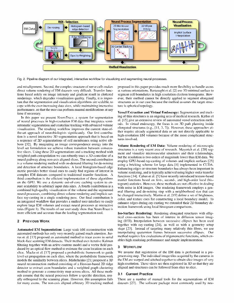
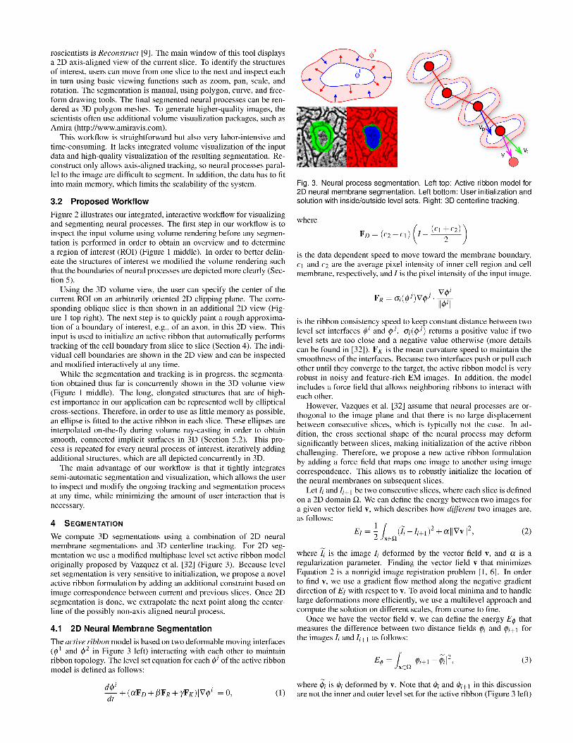
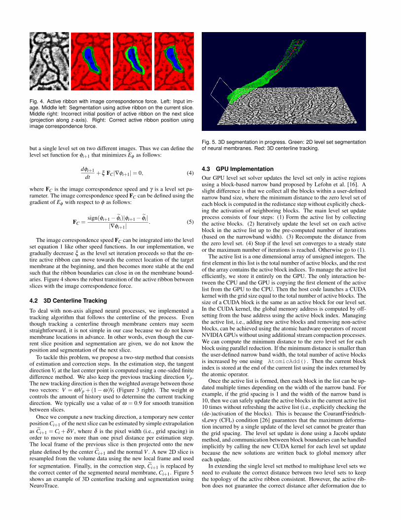
Fig. 4. Active ribbon with image correspondence force. Left: Input im-age. Middle left: Segmentation using active ribbon on the current slice.Middle right: Incorrect initial position of active ribbon on the next slice(projection along z-axis). Right: Correct active ribbon position usingimage correspondence force.

but a single level set on two different images. Thus we can define thelevel set function for φi+1 that minimizes Eφ as follows:

dφi+1

dt+ξ FC|∇φi+1|= 0, (4)

where FC is the image correspondence speed and γ is a level set pa-rameter. The image correspondence speed FC can be defined using thegradient of Eφ with respect to φ as follows:

FC =sign(φi+1− φi)|φi+1− φi|

|∇φi+1|. (5)

The image correspondence speed FC can be integrated into the levelset equation 1 like other speed functions. In our implementation, wegradually decrease ξ as the level set iteration proceeds so that the en-tire active ribbon can move towards the correct location of the targetmembrane at the beginning, and then becomes more stable at the endsuch that the ribbon boundaries can close in on the membrane bound-aries. Figure 4 shows the robust transition of the active ribbon betweenslices with the image correspondence force.

4.2 3D Centerline Tracking

To deal with non-axis aligned neural processes, we implemented atracking algorithm that follows the centerline of the process. Eventhough tracking a centerline through membrane centers may seemstraightforward, it is not simple in our case because we do not knowmembrane locations in advance. In other words, even though the cur-rent slice position and segmentation are given, we do not know theposition and segmentation of the next slice.

To tackle this problem, we propose a two-step method that consistsof estimation and correction steps. In the estimation step, the tangentdirection Vt at the last center point is computed using a one-sided finitedifference method. We also keep the previous tracking direction Vp.The new tracking direction is then the weighted average between thosetwo vectors: V = ωVp + (1−ω)Vt (Figure 3 right). The weight ωcontrols the amount of history used to determine the current trackingdirection. We typically use a value of ω = 0.9 for smooth transitionbetween slices.

Once we compute a new tracking direction, a temporary new centerposition Ci+1 of the next slice can be estimated by simple extrapolation

as Ci+1 = Ci + δV , where δ is the pixel width (i.e., grid spacing) inorder to move no more than one pixel distance per estimation step.The local frame of the previous slice is then projected onto the new

plane defined by the center Ci+1 and the normal V . A new 2D slice isresampled from the volume data using the new local frame and used

for segmentation. Finally, in the correction step, Ci+1 is replaced bythe correct center of the segmented neural membrane, Ci+1. Figure 5shows an example of 3D centerline tracking and segmentation usingNeuroTrace.

Fig. 5. 3D segmentation in progress. Green: 2D level set segmentationof neural membranes. Red: 3D centerline tracking.

4.3 GPU Implementation

Our GPU level set solver updates the level set only in active regionsusing a block-based narrow band proposed by Lefohn et al. [16]. Aslight difference is that we collect all the blocks within a user-definednarrow band size, where the minimum distance to the zero level set ofeach block is computed in the redistance step without explicitly check-ing the activation of neighboring blocks. The main level set updateprocess consists of four steps: (1) Form the active list by collectingthe active blocks. (2) Iteratively update the level set on each activeblock in the active list up to the pre-computed number of iterations(based on the narrowband width). (3) Recompute the distance fromthe zero level set. (4) Stop if the level set converges to a steady stateor the maximum number of iterations is reached. Otherwise go to (1).

The active list is a one dimensional array of unsigned integers. Thefirst element in this list is the total number of active blocks, and the restof the array contains the active block indices. To manage the active listefficiently, we store it entirely on the GPU. The only interaction be-tween the CPU and the GPU is copying the first element of the activelist from the GPU to the CPU. Then the host code launches a CUDAkernel with the grid size equal to the total number of active blocks. Thesize of a CUDA block is the same as an active block for our level set.In the CUDA kernel, the global memory address is computed by off-setting from the base address using the active block index. Managingthe active list, i.e., adding new active blocks and removing non-activeblocks, can be achieved using the atomic hardware operators of recentNVIDIA GPUs without using additional stream compaction processes.We can compute the minimum distance to the zero level set for eachblock using parallel reduction. If the minimum distance is smaller thanthe user-defined narrow band width, the total number of active blocksis increased by one using AtomicAdd(). Then the current blockindex is stored at the end of the current list using the index returned bythe atomic operator.

Once the active list is formed, then each block in the list can be up-dated multiple times depending on the width of the narrow band. Forexample, if the grid spacing is 1 and the width of the narrow band is10, then we can safely update the active blocks in the current active list10 times without refreshing the active list (i.e., explicitly checking the(de-)activation of the blocks). This is because the CourantFriedrich-sLewy (CFL) condition [26] guarantees that the maximum deforma-tion incurred by a single update of the level set cannot be greater thanthe grid spacing. The level set update is done using a Jacobi updatemethod, and communication between block boundaries can be handledimplicitly by calling the new CUDA kernel for each level set updatebecause the new solutions are written back to global memory aftereach update.

In extending the single level set method to multiphase level sets weneed to evaluate the correct distance between two level sets to keepthe topology of the active ribbon consistent. However, the active rib-bon does not guarantee the correct distance after deformation due to

the combination of various force fields. Therefore, we recompute thedistance field for each level set when the list of active blocks is up-dated. Note that we need to redistance not only on the active lists butthe complete level sets because the level sets may not share the sameactive list unless they are very close to each other. To quickly computethe distance fields we employ the GPU-based Eikonal solver by Jeonget al. [12].

We implemented the nonrigid image registration method usingsemi-implicit discretization as a two-step iterative process, updatingand smoothing the vector field v as follows:

v ← v+dt(Ii+1− Ii)∇Ii (6)

v ← G⋆v, (7)

where G is a Gaussian smoothing kernel. Equation 6 is a simple Eulerintegration that can be efficiently mapped to the GPU. To interpolate

the pixel values Ii and ∇Ii on locations defined by v we use texturehardware interpolation on the GPU. Texture memory is cached, so itis efficient for locally coherent random memory accesses. To speedup the 2D Gaussian smoothing in image space, we implemented a se-quence of 1D convolutions using shared memory and apply them alongx and y, respectively.

5 VOLUME VISUALIZATION

Volume rendering of high-resolution EM data poses several chal-lenges. EM data is extremely dense and heavily textured, exhibits acomplex structure of interconnected nerve cells, and has a low signal-to-noise ratio. Therefore, standard volume rendering results in clut-tered images that make it hard to identify regions of interest (ROIs) orto observe an ongoing segmentation.

Our visualization approach supports the inspection of data prior tosegmentation, for identifying ROIs, as well as the visualization of theongoing and final segmentation (see Figure 2). To improve the visu-alization of the raw data prior to segmentation, we have implementedon-the-fly nonlinear noise removal and edge enhancement to supportthe user in finding and selecting ROIs. Using a local histogram-basededge metric, which is only calculated on demand for currently visi-ble parts of the volume and cached for later reuse, we can enhanceimportant structures (e.g., myelinated axons) while fading out less im-portant regions. During ray-casting we use the computed edge valuesto modulate the current sample’s opacity with different user-selectableopacity weighting modes (e.g., min, max, alpha blending).

5.1 On-demand Filtering

The main motivations for on-demand filtering (i.e., noise removal andedge detection) are the flexibility offered by being able to change fil-ters and filter parameters on the fly while avoiding additional disk stor-age and bandwidth bottlenecks for terabyte-sized volume data. Weperform filtering only on blocks of the volume that are visible fromthe current viewpoint, and store the computed data directly on the GPUfor later reuse. We have implemented a caching scheme for these pre-computed blocks on the GPU to avoid costly transfers to and fromGPU memory while at the same time avoiding repetitive recalculationof filtered blocks. During visualization we display either the originalvolume, the noise-reduced data, the computed edge values, or a com-bination of the above.

Our on-demand filtering algorithm consists of several steps: (1)Detect for each block in the volume if it is visible from the currentviewpoint. (2) Build the list of blocks that need to be computed. (3)Perform noise removal filtering on selected blocks and store them inthe cache. (4) Calculate the histogram-based edge metric on selectedblocks and store those blocks in the cache. (5) High-resolution ray-casting combining edge values and original data values. The detectionof visible blocks (Step 1) is done either in a separate low-resolutionray-casting pass or included in Step 5.

5.1.1 Noise Removal

Since EM data generally exhibits a low signal-to-noise ratio we haveintegrated an on-demand noise removal filter step into our pipeline

prior to calculating the local histogram-based edge metric. We per-form the filtering only on those blocks that were marked as visibleand are not present in the cache yet. We have implemented 2D and 3DGaussian, mean, non-linear median, bilateral [31], and anisotropic dif-fusion filters [22] with user adjustable neighborhood sizes. Especiallynon-linear filters have shown good noise removal properties withoutdegrading edges in the EM data [30]. Our main objective, however,was to develop a general framework for noise removal, where addi-tional filters could be added easily. The results for each processedblock is stored in the cache and used as input for the edge detectionalgorithm.

5.1.2 Local Histogram-based Edge Detection

We use a local histogram-based edge metric to modulate the opacity ofthe EM data during raycasting. Boundaries in the volume get enhancedwhile more homogenous regions are supressed. This helps the userin navigating through the unsegmented dataset and in finding regionswhere a segmentation should be started. The edge metric is computedonly for visible blocks that are not stored in the cache yet.

Our edge detection algorithm is based on the work of Martin etal. [19] who introduced edge and boundary detection in 2D imagebased on local histograms. They did a thorough evaluation of differentbrightness, color, and texture cues for constructing a local boundarymodel, which was subsequently used to detect contours [18] in naturalimages.

In our local histogram-based edge detection approach we take ablock neighborhood around each voxel to calculate the brightness gra-dient for different directions. We separate the voxel’s neighborhoodalong the given direction into two halves and calculate the histogramin each half-space. Finally, the histogram difference is calculated us-ing the χ2 distance metric. A high difference between histograms in-dicates an abrupt change in brightness in the volume, i.e., an edge.The maximum difference value over all directions is saved as the edgevalue in the cache block. As the neighborhood size for the histogramcalculation can be adjusted to match the resolution level of the currentinput data, this approach scales to large data and to volume subdivisionschemes like octrees. Again, we have kept the implementation of ouredge detection framework as modular as possible to support addingdifferent edge detection algorithms in the future. During volume ren-dering, we fetch at each sample location the corresponding edge valueand use it to modulate the sample’s opacity and/or color. Optionally,the user can first use a windowing function on the calculated edge val-ues to further enhance the visualization.

5.1.3 Dynamic Caching

To improve the performance of our edge-based visualization schemewe have implemented a dynamic caching scheme for storing on-the-flycomputed blocks. Two caches are allocated directly on the GPU, oneto store de-noised volume blocks and the second to store blocks con-taining the calculated edge values. First, the visibility of all blocks isupdated for the current viewpoint in a first ray-casting pass and savedin a 3D array corresponding to the number of blocks in the volume.Next, all blocks are flagged as either: (1) visible, present in cache; (2)visible, not present in cache; (3) not visible, present in cache; or (4)not visible, not present in cache. Visible blocks that are already in thecache (flagged with (1)) do not need to be recomputed. Only blocksflagged with (2) need to the processed. Therefore, indices of blocksflagged with (2) are stored for later calculation (see Section 5.1.4).During filtering/edge detection the computed blocks are stored in thecorresponding cache. A small lookup table is maintained for mappingbetween block storage space in the cache to actual volume blocks asdescribed in [4]. Unused blocks are kept in the cache for later reuse(flagged with (3)). However, if cache memory gets low, unused blocksare flushed from the cache and replaced by currently visible blocks.

5.1.4 GPU Implementation

After detecting which blocks need processing, a CUDA kernel islaunched with grid size corresponding to the number of blocks thatneed to be processed. For simplicity we explain the implementation of

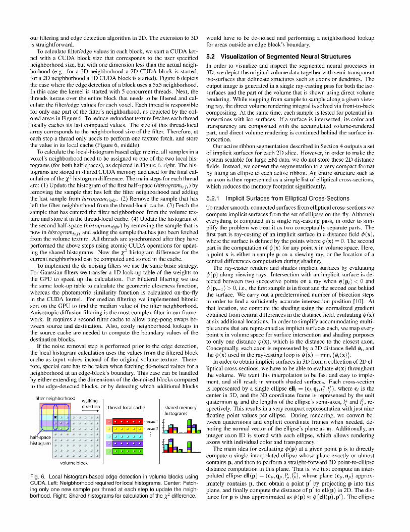
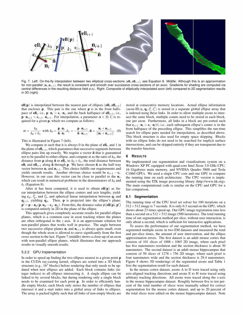
Fig. 7. Left: On-the-fly interpolation between two elliptical cross-sections (elli,elli+1), see Equation 8. Middle: Although this is an approximationfor non-parallel (ni,ni+1), the result is consistent and smooth over successive cross-sections of an axon. Gradients for shading are computed viacentral differences in the resulting distance field φ(x). Right: Composite of elliptically-interpolated axon (left) compared to 2D segmentation resultsin 3D (right).

ell(p) is interpolated between the nearest pair of ellipses (elli,elli+1)that encloses p. This pair is the one where p is in the front halfs-pace of elli, i.e., p ·ni > ci ·ni, and the back halfspace of elli+1, i.e.,p ·ni+1 < ci+1 ·ni+1. For interpolation, a parameter α ∈ [0,1] is re-quired for a given p, which we compute as follows:

α =k0

k0 + k1with k0 =

p ·ni

n ·ni,k1 =−

p ·ni+1

n ·ni+1, n =

ni +ni+1

||ni +ni+1||. (8)

This is illustrated in Figure 7 (left).

We compute α such that it is always 0 in the plane of elli, and 1 inthe plane of elli+1, which guarantees that successive segments betweenellipse pairs line up exactly. We require a vector n that is guaranteednot to be parallel to either ellipse, and compute α as the ratio of k0, thedistance from p along n to elli, to k0 + k1, the total distance betweenelli and elli+1 along n through p. We have chosen n as the half-wayvector between ni and ni+1. This choice fulfills our requirements andyields smooth results. Another obvious choice would be ci+1 − ci.However, in our case this vector can be close to parallel to the ni,which can result in numerical problems in the denominators of k0 andk1 (Equation 8).

After α has been computed, it is used to obtain ell(p) as lin-ear interpolation between the ellipse centers and axis lengths, yield-ing cp, lx

p, and lyp, and spherical linear interpolation between qi and

qi+1, yielding qp. Then, p is projected into the ellipse’s plane:

p′= p−np(p ·np−cp ·np). From this, the distance value φ(ell(p),p′

)

is computed entirely in 2D in the plane of the ellipse.

This approach gives completely accurate results for parallel ellipseplanes, which is a common case in axon tracking where the planesare often orthogonal to the z axis. It is an approximate solution fornon-parallel planes that works well in practice. The angle betweentwo successive ellipse planes ni and ni+1 is always quite small, eventhough the whole axon is allowed to curve significantly from the firstcross-section to the last. Figure 7 (middle) shows a close-up of an axonwith non-parallel ellipse planes, which illustrates that our approachresults in visually smooth results.

5.2.2 GPU Implementation

In order to speed up finding the two ellipses nearest to a given point p

in the CUDA ray-casting kernel, ellipses are sorted into a 3D blockstructure (e.g., 163 blocks) before rendering that only needs to be up-dated when new ellipses are added. Each block contains links (in-teger indices) to all ellipses intersecting it. A single ellipse can belinked to by several blocks, but during rendering only a single blockneeds to be examined for each point p. In order to efficiently han-dle empty blocks, each block only stores the number of ellipses thatintersect it and a start index into a global array of links to ellipses.The array is packed tightly such that all links of non-empty blocks are

stored at consecutive memory locations. Actual ellipse information(axon-ID,ci,qi, l

xi , l

yi ) is stored in a separate global ellipse array that

is indexed using these links. In order to allow multiple axons to inter-sect the same block, multiple counts need to be stored in each block,one per axon. Furthermore, all links in a block are pre-sorted suchthat ci+1 ·ni > ci ·ni∀i, i.e., each subsequent ellipse’s center is in thefront halfspace of the preceding ellipse. This simplifies the run-timesearch for ellipse pairs needed for interpolation, as described above.This block structure is also used for empty space skipping. Blockswith no ellipse links do not need to be searched for implicit surfaceintersections, and can be skipped entirely if they are transparent due tothe transfer function.

6 RESULTS

We implemented our segmentation and visualizations system on aWindows XP PC equipped with quad-core Intel Xeon 3.0 GHz CPU,16 Gigabytes main memory, and NVIDIA Quadro 5800 and TeslaC1060 GPUs. We used a single CPU core and one GPU to comparethe running time on each architecture. The CPU version is imple-mented using the ITK image processing library (http://www.itk.org).The main computational code is similar on the CPU and GPU for afair comparison.

6.1 Segmentation

The running time of the CPU level set solver for 100 iterations on a512×512 image is 7 seconds. It is only 0.3 second on the GPU, whichshows about 23 times speed-up. Our GPU image registration runs lessthan a second on a 512×512 image (500 iterations). The total runningtime of our segmentation method per slice, without user interaction, isonly about a second, which is sufficient for interactive applications.

To assess the performance of our segmentation method, we havesegmented multiple axons in two EM datasets and measured the totaland per-slice times, the amount of user intervention, and the ellipseapproximation errors. The first dataset is an adult mouse cortex thatconsists of 101 slices of 1008× 1065 2D image, where each pixelhas five nanometers resolution and the section thickness is about 30nanometers. The second dataset is an adult mouse hippocampus thatconsists of 50 slices of 1278× 756 2D image, where each pixel isfour nanometers wide and the section thickness is 29.4 nanometers.Figure 8 shows 3D renderings of the segmented axons and Table 1lists the segmentation result for each dataset.

In the mouse cortex dataset, axons A to D were traced using onlyaxis-aligned tracking directions and axons E to H were traced usingarbitrary tracking directions. All axons were traced along the z-axisin the mouse hippocampus dataset. Roughly between five to ten per-cent of the total number of slices were manually edited for correctsegmentation for the mouse cortex dataset, and up to 20 percent ofthe total slices were edited on the mouse hippocampus dataset. Note

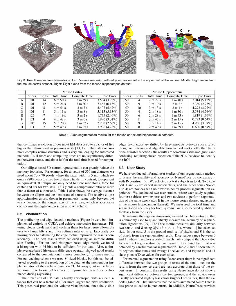
Fig. 8. Result images from NeuroTrace. Left: Volume rendering with edge enhancement in the upper part of the volume. Middle: Eight axons fromthe mouse cortex dataset. Right: Eight axons from the mouse hippocampus dataset.

Mouse Cortex Mouse Hippocampus

Slices Edits Total Time Compute Time Ellipse Error Slices Edits Total Time Compute Time Ellipse Error

A 101 14 6 m 50 s 3 m 59 s 3.584 (3.98%) 50 4 2 m 27 s 1 m 40 s 7.014 (5.12%)B 101 12 5 m 24 s 3 m 30 s 7.468 (6.13%) 50 9 3 m 19 s 2 m 2 s 2.380 (2.73%)C 101 8 4 m 54 s 3 m 7 s 5.407 (5.62%) 50 10 3 m 13 s 2 m 1 s 4.292 (3.97%)D 101 11 5 m 11 s 3 m 8 s 5.115 (5.13%) 50 4 2 m 18 s 1 m 30 s 3.534 (4.76%)E 127 7 4 m 19 s 3 m 2 s 1.775 (2.46%) 50 6 2 m 28 s 1 m 43 s 1.819 (1.76%)F 121 4 4 m 42 s 3 m 0 s 1.890 (3.01%) 50 11 3 m 47 s 2 m 15 s 0.773 (0.64%)G 105 15 5 m 20 s 2 m 52 s 2.230 (2.66%) 50 9 3 m 14 s 2 m 15 s 4.966 (3.37%)H 111 7 5 m 49 s 3 m 35 s 3.996 (4.28%) 50 8 2 m 49 s 1 m 39 s 0.630 (0.67%)

Table 1. Axon segmentation results for the mouse cortex and hippocampus datasets.

that the image resolution of our input EM data is up to a factor of fivehigher than those used in previous work [13, 17]. The data containsmore complex neural structures and is very challenging for automatedmethods. Total times and computing times are not significantly differ-ent between axons, and about half of the total time is used for compu-tation.

Our ellipse-based 3D neuron representation can greatly reduce thememory footprint. For example, for an axon of 350 nm diameter weneed about 70× 70 pixels where the pixel width is 5 nm, which re-quires 9800 floats to store two distance fields. In contrast, to representan equivalent 3D ellipse we only need to store nine floats, three forcenter and six for two axis. This yields a compression ratio of morethan a factor of a thousand. Table 1 also shows the average distancebetween the ellipse and the membrane of neurons. The relative ellipseapproximation errors, shown in parenthesis, range only between 0.6to six percent of the longest axis of the ellipse, which is acceptableconsidering the high compression ratio we achieve.

6.2 Visualization

The prefiltering and edge-detection methods (Figure 9) were both im-plemented entirely in CUDA and achieve interactive framerates. Fil-tering blocks on-demand and caching them for later reuse allows theuser to change filters and filter settings interactively. Especially de-noising prior to calculating the edge metric improved the results con-siderably. The best results were achieved using anisotropic diffu-sion filtering. For our local histogram-based edge metric we founda histogram with 64 bins to be sufficient for our data. Also, a sim-ple average-based histogram difference operator showed good resultscompared to the computationally more complex χ2 distance metric.

For our caching scheme we used 83 sized blocks, but this can be ad-justed according to the resolution of the data. At the moment our im-plementation of the cache is based on CUDA arrays, but in the futurewe would like to use 3D textures to improve tri-linear filter perfor-mance during raycasting.

The dimension of EM data is highly anisotropic, with z-slice dis-tances that can be a factor of 10 or more larger than pixel resolution.This poses real problems for volume visualization, since the visible

edges from axons are shifted by large amounts between slices. Eventhough our filtering and edge detection method works better than tradi-tional transfer functions, the results are sometimes still ambiguous andconfusing, requiring closer inspection of the 2D slice views to identifythe ROI.

6.3 User Study

We have conducted informal user studies of our segmentation methodto assess the usability and accuracy of NeuroTrace by comparing itwith Reconstruct [9]. We selected six test subjects in total. Two (Ex-pert 1 and 2) are expert neuroscientists, and the other four (Novice1 to 4) are novices with no previous neural process segmentation ex-perience. We conducted two user studies, where each study requiredfour test subjects (two experts and two novices) to perform segmenta-tion of the same axon (axon E in the mouse cortex dataset and axon Ain the mouse hippocampus dataset). We measured the total time andsegmentation accuracy for both systems. We also received qualitativefeedback from the users.

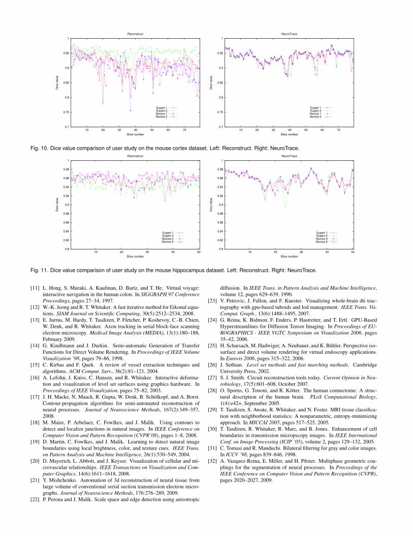
To measure the segmentation error, we used the Dice metric [8] thatis commonly used to quantitatively measure the accuracy of segmen-tation algorithms [29]. The Dice metric measures similarity betweentwo sets A and B using 2|A∩B|/(|A|+ |B|), where | · | indicates setsize. In our case, A is the ground truth set of pixels, and B is the setof pixels from the segmentation result. Dice values range between 0and 1, where 1 implies a perfect match. We compute the Dice valuefor each 2D segmentation by comparing it to ground truth that wasobtained by careful manual segmentation. Table 2 and 3 show the to-tal segmentation times and average Dice values, and Figure 10 and 11show plots of Dice values for each slice.

For manual segmentation using Reconstruct there is no significantdifference between the two groups in terms of the total time, but theresults from the novice users are less accurate than those of the ex-pert users. In contrast, the results using NeuroTrace do not show asignificant difference between the two groups, and the novice usersusually generated slightly less errors (higher Dice values) than the ex-perts (Table 2). That indicates that the semi-automated NeuroTrace isless prone to lead to human errors. In addition, NeuroTrace provides

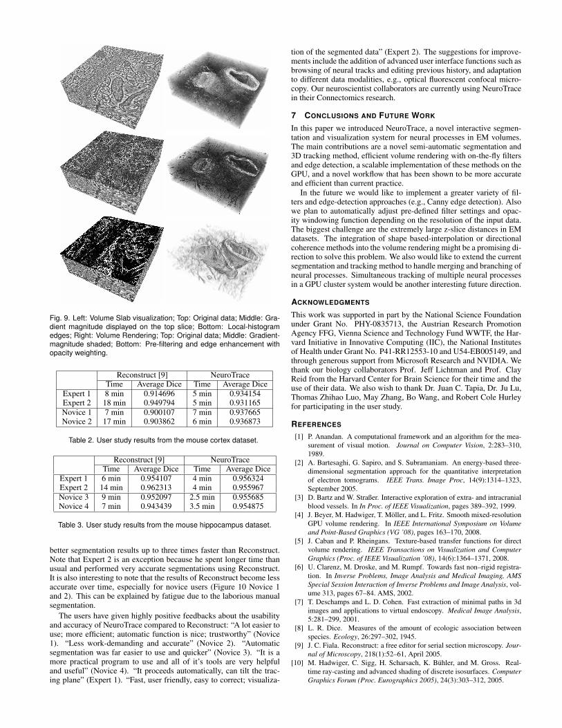
Fig. 9. Left: Volume Slab visualization; Top: Original data; Middle: Gra-dient magnitude displayed on the top slice; Bottom: Local-histogramedges; Right: Volume Rendering; Top: Original data; Middle: Gradient-magnitude shaded; Bottom: Pre-filtering and edge enhancement withopacity weighting.

Reconstruct [9] NeuroTraceTime Average Dice Time Average Dice

Expert 1 8 min 0.914696 5 min 0.934154Expert 2 18 min 0.949794 5 min 0.931165

Novice 1 7 min 0.900107 7 min 0.937665Novice 2 17 min 0.903862 6 min 0.936873

Table 2. User study results from the mouse cortex dataset.

Reconstruct [9] NeuroTraceTime Average Dice Time Average Dice

Expert 1 6 min 0.954107 4 min 0.956324Expert 2 14 min 0.962313 4 min 0.955967

Novice 3 9 min 0.952097 2.5 min 0.955685Novice 4 7 min 0.943439 3.5 min 0.954875

Table 3. User study results from the mouse hippocampus dataset.

better segmentation results up to three times faster than Reconstruct.Note that Expert 2 is an exception because he spent longer time thanusual and performed very accurate segmentations using Reconstruct.It is also interesting to note that the results of Reconstruct become lessaccurate over time, especially for novice users (Figure 10 Novice 1and 2). This can be explained by fatigue due to the laborious manualsegmentation.

The users have given highly positive feedbacks about the usabilityand accuracy of NeuroTrace compared to Reconstruct: “A lot easier touse; more efficient; automatic function is nice; trustworthy” (Novice1). “Less work-demanding and accurate” (Novice 2). “Automaticsegmentation was far easier to use and quicker” (Novice 3). “It is amore practical program to use and all of it’s tools are very helpfuland useful” (Novice 4). “It proceeds automatically, can tilt the trac-ing plane” (Expert 1). “Fast, user friendly, easy to correct; visualiza-

tion of the segmented data” (Expert 2). The suggestions for improve-ments include the addition of advanced user interface functions such asbrowsing of neural tracks and editing previous history, and adaptationto different data modalities, e.g., optical fluorescent confocal micro-copy. Our neuroscientist collaborators are currently using NeuroTracein their Connectomics research.

7 CONCLUSIONS AND FUTURE WORK

In this paper we introduced NeuroTrace, a novel interactive segmen-tation and visualization system for neural processes in EM volumes.The main contributions are a novel semi-automatic segmentation and3D tracking method, efficient volume rendering with on-the-fly filtersand edge detection, a scalable implementation of these methods on theGPU, and a novel workflow that has been shown to be more accurateand efficient than current practice.

In the future we would like to implement a greater variety of fil-ters and edge-detection approaches (e.g., Canny edge detection). Alsowe plan to automatically adjust pre-defined filter settings and opac-ity windowing function depending on the resolution of the input data.The biggest challenge are the extremely large z-slice distances in EMdatasets. The integration of shape based-interpolation or directionalcoherence methods into the volume rendering might be a promising di-rection to solve this problem. We also would like to extend the currentsegmentation and tracking method to handle merging and branching ofneural processes. Simultaneous tracking of multiple neural processesin a GPU cluster system would be another interesting future direction.

ACKNOWLEDGMENTS

This work was supported in part by the National Science Foundationunder Grant No. PHY-0835713, the Austrian Research PromotionAgency FFG, Vienna Science and Technology Fund WWTF, the Har-vard Initiative in Innovative Computing (IIC), the National Institutesof Health under Grant No. P41-RR12553-10 and U54-EB005149, andthrough generous support from Microsoft Research and NVIDIA. Wethank our biology collaborators Prof. Jeff Lichtman and Prof. ClayReid from the Harvard Center for Brain Science for their time and theuse of their data. We also wish to thank Dr. Juan C. Tapia, Dr. Ju Lu,Thomas Zhihao Luo, May Zhang, Bo Wang, and Robert Cole Hurleyfor participating in the user study.

REFERENCES

[1] P. Anandan. A computational framework and an algorithm for the mea-

surement of visual motion. Journal on Computer Vision, 2:283–310,

1989.

[2] A. Bartesaghi, G. Sapiro, and S. Subramaniam. An energy-based three-

dimensional segmentation approach for the quantitative interpretation

of electron tomograms. IEEE Trans. Image Proc, 14(9):1314–1323,

September 2005.

[3] D. Bartz and W. Straßer. Interactive exploration of extra- and intracranial

blood vessels. In In Proc. of IEEE Visualization, pages 389–392, 1999.

[4] J. Beyer, M. Hadwiger, T. Moller, and L. Fritz. Smooth mixed-resolution

GPU volume rendering. In IEEE International Symposium on Volume

and Point-Based Graphics (VG ’08), pages 163–170, 2008.

[5] J. Caban and P. Rheingans. Texture-based transfer functions for direct

volume rendering. IEEE Transactions on Visualization and Computer

Graphics (Proc. of IEEE Visualization ’08), 14(6):1364–1371, 2008.

[6] U. Clarenz, M. Droske, and M. Rumpf. Towards fast non–rigid registra-

tion. In Inverse Problems, Image Analysis and Medical Imaging, AMS

Special Session Interaction of Inverse Problems and Image Analysis, vol-

ume 313, pages 67–84. AMS, 2002.

[7] T. Deschamps and L. D. Cohen. Fast extraction of minimal paths in 3d

images and applications to virtual endoscopy. Medical Image Analysis,

5:281–299, 2001.

[8] L. R. Dice. Measures of the amount of ecologic association between

species. Ecology, 26:297–302, 1945.

[9] J. C. Fiala. Reconstruct: a free editor for serial section microscopy. Jour-

nal of Microscopy, 218(1):52–61, April 2005.

[10] M. Hadwiger, C. Sigg, H. Scharsach, K. Buhler, and M. Gross. Real-

time ray-casting and advanced shading of discrete isosurfaces. Computer

Graphics Forum (Proc. Eurographics 2005), 24(3):303–312, 2005.

0.7

0.75

0.8

0.85

0.9

0.95

1

10 20 30 40 50 60 70

Dic

e v

alu

e

Slice number

Reconstruct

Expert 1Expert 2Novice 1Novice 2

0.7

0.75

0.8

0.85

0.9

0.95

1

10 20 30 40 50 60 70

Dic

e v

alu

e

Slice number

NeuroTrace

Expert 1Expert 2Novice 1Novice 2

Fig. 10. Dice value comparison of user study on the mouse cortex dataset. Left: Reconstruct. Right: NeuroTrace.

0.8

0.82

0.84

0.86

0.88

0.9

0.92

0.94

0.96

0.98

1

10 20 30 40 50

Dic

e v

alu

e

Slice number

Reconstruct

Expert 1Expert 2Novice 3Novice 4

0.8

0.82

0.84

0.86

0.88

0.9

0.92

0.94

0.96

0.98

1

10 20 30 40 50

Dic

e v

alu

e

Slice number

NeuroTrace

Expert 1Expert 2Novice 3Novice 4

Fig. 11. Dice value comparison of user study on the mouse hippocampus dataset. Left: Reconstruct. Right: NeuroTrace.

[11] L. Hong, S. Muraki, A. Kaufman, D. Bartz, and T. He. Virtual voyage:

interactive navigation in the human colon. In SIGGRAPH 97 Conference

Proceedings, pages 27–34, 1997.

[12] W.-K. Jeong and R. T. Whitaker. A fast iterative method for Eikonal equa-

tions. SIAM Journal on Scientific Computing, 30(5):2512–2534, 2008.

[13] E. Jurrus, M. Hardy, T. Tasdizen, P. Fletcher, P. Koshevoy, C.-B. Chien,

W. Denk, and R. Whitaker. Axon tracking in serial block-face scanning

electron microscopy. Medical Image Analysis (MEDIA), 13(1):180–188,

February 2009.

[14] G. Kindlmann and J. Durkin. Semi-automatic Generation of Transfer

Functions for Direct Volume Rendering. In Proceedings of IEEE Volume

Visualization ’98, pages 79–86, 1998.

[15] C. Kirbas and F. Quek. A review of vessel extraction techniques and

algorithms. ACM Comput. Surv., 36(2):81–121, 2004.

[16] A. Lefohn, J. Kniss, C. Hansen, and R. Whitaker. Interactive deforma-

tion and visualization of level set surfaces using graphics hardware. In

Proceedings of IEEE Visualization, pages 75–82, 2003.

[17] J. H. Macke, N. Maack, R. Gupta, W. Denk, B. Scholkopf, and A. Borst.

Contour-propagation algorithms for semi-automated reconstruction of

neural processes. Journal of Neuroscience Methods, 167(2):349–357,

2008.

[18] M. Maire, P. Arbelaez, C. Fowlkes, and J. Malik. Using contours to

detect and localize junctions in natural images. In IEEE Conference on

Computer Vision and Pattern Recognition (CVPR’08), pages 1–8, 2008.

[19] D. Martin, C. Fowlkes, and J. Malik. Learning to detect natural image

boundaries using local brightness, color, and texture cues. IEEE Trans.

on Pattern Analysis and Machine Intelligence, 26(1):530–549, 2004.

[20] D. Mayerich, L. Abbott, and J. Keyser. Visualization of cellular and mi-

crovascular relationships. IEEE Transactions on Visualization and Com-

puter Graphics, 14(6):1611–1618, 2008.

[21] Y. Mishchenko. Automation of 3d reconstruction of neural tissue from

large volume of conventional serial section transmission electron micro-

graphs. Journal of Neuroscience Methods, 176:276–289, 2009.

[22] P. Perona and J. Malik. Scale space and edge detection using anisotropic

diffusion. In IEEE Trans. in Pattern Analysis and Machine Intelligence,

volume 12, pages 629–639, 1990.

[23] V. Petrovic, J. Fallon, and F. Kuester. Visualizing whole-brain dti trac-

tography with gpu-based tuboids and lod management. IEEE Trans. Vis.

Comput. Graph., 13(6):1488–1495, 2007.

[24] G. Reina, K. Bidmon, F. Enders, P. Hastreiter, and T. Ertl. GPU-Based

Hyperstreamlines for Diffusion Tensor Imaging. In Proceedings of EU-

ROGRAPHICS - IEEE VGTC Symposium on Visualization 2006, pages

35–42, 2006.

[25] H. Scharsach, M. Hadwiger, A. Neubauer, and K. Buhler. Perspective iso-

surface and direct volume rendering for virtual endoscopy applications.

In Eurovis 2006, pages 315–322, 2006.

[26] J. Sethian. Level set methods and fast marching methods. Cambridge

University Press, 2002.

[27] S. J. Smith. Circuit reconstruction tools today. Current Opinion in Neu-

robiology, 17(5):601–608, October 2007.

[28] O. Sporns, G. Tononi, and R. Kotter. The human connectome: A struc-

tural description of the human brain. PLoS Computational Biology,

1(4):e42+, September 2005.

[29] T. Tasdizen, S. Awate, R. Whitaker, and N. Foster. MRI tissue classifica-

tion with neighborhood statistics: A nonparametric, entropy-minimizing

approach. In MICCAI 2005, pages 517–525, 2005.

[30] T. Tasdizen, R. Whitaker, R. Marc, and B. Jones. Enhancement of cell

boundaries in transmission micropscopy images. In IEEE International

Conf. on Image Processing (ICIP ’05), volume 2, pages 129–132, 2005.

[31] C. Tomasi and R. Manduchi. Bilateral filtering for gray and color images.

In ICCV ’98, pages 839–846, 1998.

[32] A. Vazquez-Reina, E. Miller, and H. Pfister. Multiphase geometric cou-

plings for the segmentation of neural processes. In Proceedings of the

IEEE Conference on Computer Vision and Pattern Recognition (CVPR),

pages 2020–2027, 2009.