Scalable parallel methods for monolithic coupling in

fluid-structure interaction with application to blood flow

modeling

Andrew T. Barker∗,a, Xiao-Chuan Caib

aDepartment of Applied Mathematics, University of Colorado, 526 UCB, Boulder, CO

80309-0526bDepartment of Computer Science, University of Colorado, 430 UCB, Boulder, CO

80309-0430

Abstract

We introduce and study numerically a scalable parallel finite element solverfor the simulation of blood flow in compliant arteries. The incompressibleNavier-Stokes equations are used to model the fluid and coupled to an incom-pressible linear elastic model for the blood vessel walls. Our method featuresan unstructured dynamic mesh capable of modeling complicated geometries,an arbitrary Lagrangian-Eulerian framework that allows for large displace-ments of the moving fluid domain, monolithic coupling between the fluid andstructure equations, and fully implicit time discretization. Simulations basedon blood vessel geometries derived from patient-specific clinical data are per-formed on large supercomputers using scalable Newton-Krylov algorithmspreconditioned with an overlapping restricted additive Schwarz method thatpreconditions the entire fluid-structure system together. The algorithm isshown to be robust and scalable for a variety of physical parameters, scalingto hundreds of processors and millions of unknowns.

Key words: fluid-structure interaction, blood flow, mesh movement,restricted additive Schwarz, domain decomposition, parallel computing

This research was supported in part by DOE under DE-FC02-04ER25595, and in partby NSF under grants CCF-0634894, and CNS-0722023, and DMS-0913089

∗Corresponding author.Email addresses: andrew.barker@colorado.edu (Andrew T. Barker),

cai@cs.colorado.edu (Xiao-Chuan Cai)

Preprint submitted to Journal of Computational Physics September 24, 2009

1. Introduction

In this work we develop a scalable parallel framework for simulating fluid-structure interaction. Fluid-structure interaction is an important concern inmany applications, including aircraft design and civil engineering, but theapplication area we focus on here is the simulation of blood flow in humanarteries.

Artery disease is the leading cause of death in developed nations, and bysome accounts is the leading cause of death worldwide [35]. Artery disease isclosely associated with flow properties of the blood and with the interactionbetween the blood and the vessel wall. In particular, areas of turbulence, flowrecirculation, or places where the artery wall is subject to low or oscillatingshear stress are at higher risk for plaque formation and disease. Accuratemodeling of these flow characteristics might enable better prediction of whenand where artery disease will occur and lead to more accurate, less invasive,and more timely treatment [43].

Unfortunately, the blood flow problem is difficult from both a modelingand a computational perspective. Good overviews of the problem can befound in [17, 43]. The main challenge we are concerned with here is theeffective coupling of the fluid and the structure in a stable and scalable man-ner. The fluid-structure coupling in arteries is strong, the structure and thefluid domain deform significantly, and the coupling is essential to describ-ing the behavior of the system, which makes the blood flow problem a goodapplication for our method.

Because of our focus, certain parts of our model are at this point physi-cally unrealistic. In particular, all our simulations are 2D, we model arterywalls as an incompressible linear elastic solid, and our outlet boundary con-ditions are simplistic. But we demonstrate that our method has attractiveconvergence properties and good scalability, and even at this stage we canqualitatively reproduce some of the more important physical aspects of bloodflow in compliant arteries and quantitatively reproduce results found in theliterature.

Blood is a viscous shear-thinning fluid, and it is inhomogeneous, contain-ing a significant proportion of non-fluid particles (blood cells and platelets).At physiological conditions it can be assumed to be incompressible. Mostmodeling also makes the assumption that blood is a Newtonian fluid, whichis a reasonable assumption in large arteries but begins to break down insmaller vessels, where the shear-thinning properties of blood become more

2

apparent [17].Artery walls are a complex tissue with three layers, each with different

non-isotropic material properties. Finding and validating accurate physicalmodels for this tissue has been the focus of a lot of effort [26, 50].

A moving artery wall implies a moving fluid domain, which means thatthe computational mesh for the fluid deforms. The displacement of the fluidmesh forms a third field of solution variables, and the governing equationsfor this field are another aspect that must be modeled. The goal is to providesmooth, well-conditioned elements as the fluid domain deforms at minimalcomputational cost. One approach is to simply say the mesh displacementsmust satisfy the Laplace equation, as in [36], but it is possible to modelthe mesh as a pseudo-structural system with a time-dependent momentumequation [15, 16].

There are three general approaches to fluid-structure coupling. The firstapproach is explicit coupling, in which the fluid and structure subproblemsare solved separately, each one using as boundary conditions results from theother’s previous time step. This approach does not guarantee any consistencyat the fluid-structure interface, and is unstable unless time steps are verysmall. The second approach is iterative coupling, where at each time stepthe fluid and structure subproblems are each solved multiple times, updatingeach other’s boundary conditions, until some desired tolerance is reached,at which point you can advance to the next time step [36, 20, 30, 46, 47].Iterative coupling, however, can also become unstable for large time steps,and in some cases can reduce the order of accuracy of the time-steppingalgorithm [33]. Finally, fluid and structure can be coupled monolithically,which means that a single system contains all variables and is solved at oncewith coupling conditions enforced strongly as part of the algebraic system[6, 7, 19, 23, 24, 25, 28, 48].

One of the primary motivations for the explicit or iterative approaches isthe ability to use existing fluid and structure codes from off the shelf, ratherthan developing a separate fluid-structure interaction code. The advantageof monolithic coupling is better and more robust convergence behavior for avariety of parameters. Our approach uses monolithic coupling.

Little work on the blood flow simulation problem makes explicit refer-ence to parallel performance and scalability, or to the particular solutionalgorithms that are employed. In particular, the research involving the bestphysical modeling of the problem says very little about the computationalefficiency of the algorithms employed [5, 7, 19]. In contrast, the work that

3

Ωs

Γw

Γi Γo

Ωf(t)

Γsn

Γsd

Γsd

ΓsdΓsn Γsd

Γw

Ωs

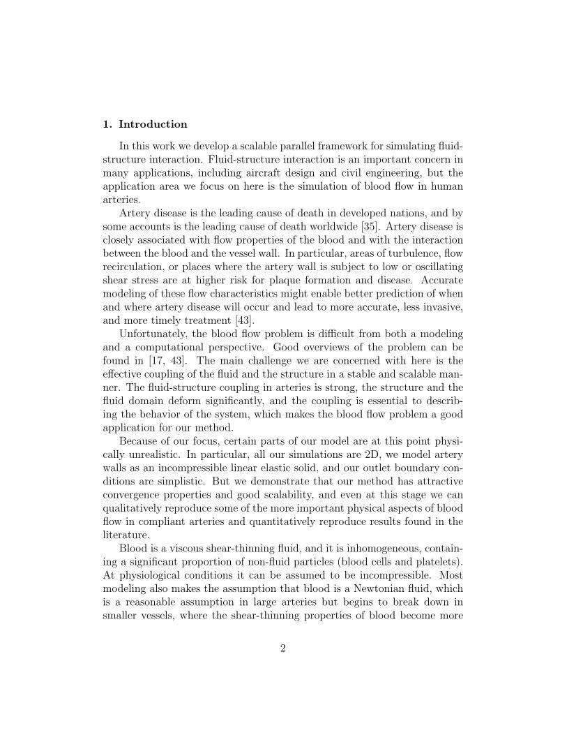
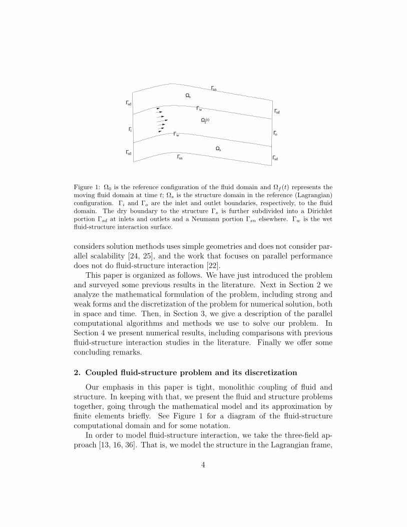
Figure 1: Ω0 is the reference configuration of the fluid domain and Ωf (t) represents themoving fluid domain at time t; Ωs is the structure domain in the reference (Lagrangian)configuration. Γi and Γo are the inlet and outlet boundaries, respectively, to the fluiddomain. The dry boundary to the structure Γs is further subdivided into a Dirichletportion Γsd at inlets and outlets and a Neumann portion Γsn elsewhere. Γw is the wetfluid-structure interaction surface.

considers solution methods uses simple geometries and does not consider par-allel scalability [24, 25], and the work that focuses on parallel performancedoes not do fluid-structure interaction [22].

This paper is organized as follows. We have just introduced the problemand surveyed some previous results in the literature. Next in Section 2 weanalyze the mathematical formulation of the problem, including strong andweak forms and the discretization of the problem for numerical solution, bothin space and time. Then, in Section 3, we give a description of the parallelcomputational algorithms and methods we use to solve our problem. InSection 4 we present numerical results, including comparisons with previousfluid-structure interaction studies in the literature. Finally we offer someconcluding remarks.

2. Coupled fluid-structure problem and its discretization

Our emphasis in this paper is tight, monolithic coupling of fluid andstructure. In keeping with that, we present the fluid and structure problemstogether, going through the mathematical model and its approximation byfinite elements briefly. See Figure 1 for a diagram of the fluid-structurecomputational domain and for some notation.

In order to model fluid-structure interaction, we take the three-field ap-proach [13, 16, 36]. That is, we model the structure in the Lagrangian frame,

4

and we would like to model the fluid in the Eulerian frame, but since thefluid domain is moving with time, we are forced instead to consider the arbi-trary Lagrangian-Eulerian framework [11, 14]. Then our three fields are thestructure, the fluid, and the moving mesh for the ALE formulation of themoving fluid domain.

For the fluid in Ωf we use the incompressible Navier-Stokes equationswritten in the ALE frame

∂uf

∂t

∣

∣

∣

∣

Y

+ [(uf − ωg) · ∇]uf +1

ρf

∇pf = νf∆uf + ff (1)

∇ · uf = 0 (2)

where ρf is the fluid density, νf is the kinematic viscosity, ωg = ∂xf/∂t is thevelocity of the moving mesh and where the Y indicates that the time deriva-tive is to be taken with respect to the ALE coordinates, not the Euleriancoordinates.

The displacement of the structure in Ωs is governed by a modified equa-tion of incompressible linear elasticity,

ρs

∂2xs

∂t2+ ∇ · σs − β

∂

∂t∆xs + γxs = fs (3)

∇ · xs = 0 (4)

where σs = −psI + µs(∇xs + ∇xTs ) is the Cauchy stress tensor for the in-

compressible structure. In a few cases we use compressible linear elasticity,where (4) is modified to read ∇ · xs + ps/λs = 0. The Lame parametersλs and µs are properties of the physical material under consideration, β isa visco-elastic damping parameter, and the γ term is used to represent aradially symmetric artery in two dimensions [2, 34]. For the moving meshwe simply make the fluid mesh displacements satisfy a harmonic extensionof the moving fluid-structure boundary

∆xf = 0. (5)

The assumption that blood is a viscous Newtonian fluid is a good one forlarge arteries, which is where we focus our analysis. The linear elastic modelwe use for the artery wall is not such a good model, but it has certainly beenused before [27, 42, 44], and is adequate as long as the wall deformation isnot too large. The choice of model for the moving fluid mesh is not physically

5

Figure 2: An undeformed fluid mesh in the reference configuration on the right, comparedto the deformed mesh at systole on the right. This simulation is done with a low value ofthe Young’s modulus E and a high inlet velocity to exaggerate the deformation of the fluiddomain. The mesh conditioning remains quite acceptable even under large deformation.

important, but it does have implications in terms of how much deformationthe solver can handle and if the solver becomes ill-conditioned (because of awarped fluid mesh) as the deformation increases. We find that our method,though it is simple, performs quite well, see Figure 2.

In addition to the equations above, we need boundary conditions, and,much more importantly, coupling conditions at the fluid-structure interface.These coupling conditions are

uf =∂xs

∂t(6)

which insures continuity of velocity at the wet surface and is the general-ization of a no-slip boundary condition for the fluid to the case of a movingboundary,

σs · n = −σf · n (7)

which enforces continuity of traction forces on the boundary, representing inparticular the force the fluid imparts on the structure, and

xf = xs. (8)

which represents the computational mesh for the fluid matching the struc-ture displacement at the boundary, allowing the structure to maintain a

6

Lagrangian description and defining the ALE description for the fluid. Equa-tion (7) in practice comes in as a (solution-dependent) Neumann-type condi-tion on the right-hand side of the structure equations, while (6) is a (again,solution-dependent) Dirichlet condition on the fluid equations.

We solve the above equations with the finite element method, discretiz-ing in space with the LBB-stable Q2 − Q1 element. To fully develop thealgorithm, we should derive the weak form of the equations, including testfunctions and function spaces, and from that derive the definitions of all thematrix operators and finite-dimensional approximations that appear. Thisdevelopment, however, is entirely standard, and so here we skip directly tothe semi-discrete form which is continuous in time and discrete in space.Those interested in the details should see [4]. The semi-discrete form is

Mf

du

dt+ B(u)u + Kfu − QT

f pf = 0 (9)

Qfu = 0 (10)

dxs

dt= xs (11)

Ms

dxs

dt+ βKsxs + Ksxs + γMsxs + QT

s ps = Auu + Appf (12)

Qsxs = 0 (13)

Kmxf = 0, (14)

together with the discretized coupling conditions uf = xs and xf = xs onΓw, corresponding to (6) and (8). Here we have two saddle-point problemsimbedded in one large, monolithically coupled system. We have reduced thestructure equations from second order to first order in time, by doubling thenumber of degrees of freedom (we keep track of both structure displacementxs and velocity xs), in preparation for the time discretization. Note theright-hand side of this equation, where the terms Au and Ap are introducedto account for the traction matching in fluid-structure interaction; that is,fluid solution variables are being used to generate a Neumann force on thestructure.

Our time discretization is fully implicit, and the preferred method is thesecond-order trapezoid rule, although our implementation is capable of fallingback on a backward Euler method. The trapezoid rule has sometimes beenfound to be unstable over long time integrations for nonlinear problems (seefor example [21]), but in our case we have not seen instability in any of our

7

tests. We use the same time-stepping scheme for both the fluid and thestructure, so we can simply enforce the coupling at each timestep. We canwrite the time-stepping scheme for the entire monolithically coupled systemas

Mn+1yn+1 − Mnyn −∆t

2(Kn+1yn+1 + Knyn) −

∆t

2(F n+1 + F n) = 0 (15)

where

yn =

unf

∆tpnf

xnf

xns

xsn

∆tpns

, M =

Mf

IMs

, (16)

K =

−B − Kf −(1/∆t)QTf

(1/∆t)Qf

Km

I−Au −Ap −Ks −(1/∆t)QT

s

(1/∆t)Qs

. (17)

Though written in matrix form, many of the operators above are nonlinear.In particular the B term depends on uf , and the Kf ,Mf and Q terms dependon the moving mesh xf . This implies that we have a Jacobian of the form

J =

Jf QTf Zm

−Qf Zc

−(∆t/2)Km

I (∆t/2)I(∆t/2)Au (∆t/2)Ap −(∆t/2)Ks Ms QT

s

−Qs

.

(18)Here Jf = Mf + (∆t/2)Kf + (∆t/2)Jf and Jf is the Jacobian derivativematrix of the nonlinear term Buf with respect to the fluid velocity variablesuf . Similarly, Zm and Zc are the derivatives of the first and second rows,respectively, of (15) with respect to the variables xf . For more detail on thederivation and form of Zm, Zc see Appendix A and [18].

8

−0.6 −0.4 −0.2 0 0.2 0.4 0.6 0.8 1−3.5

−3

−2.5

−2

−1.5

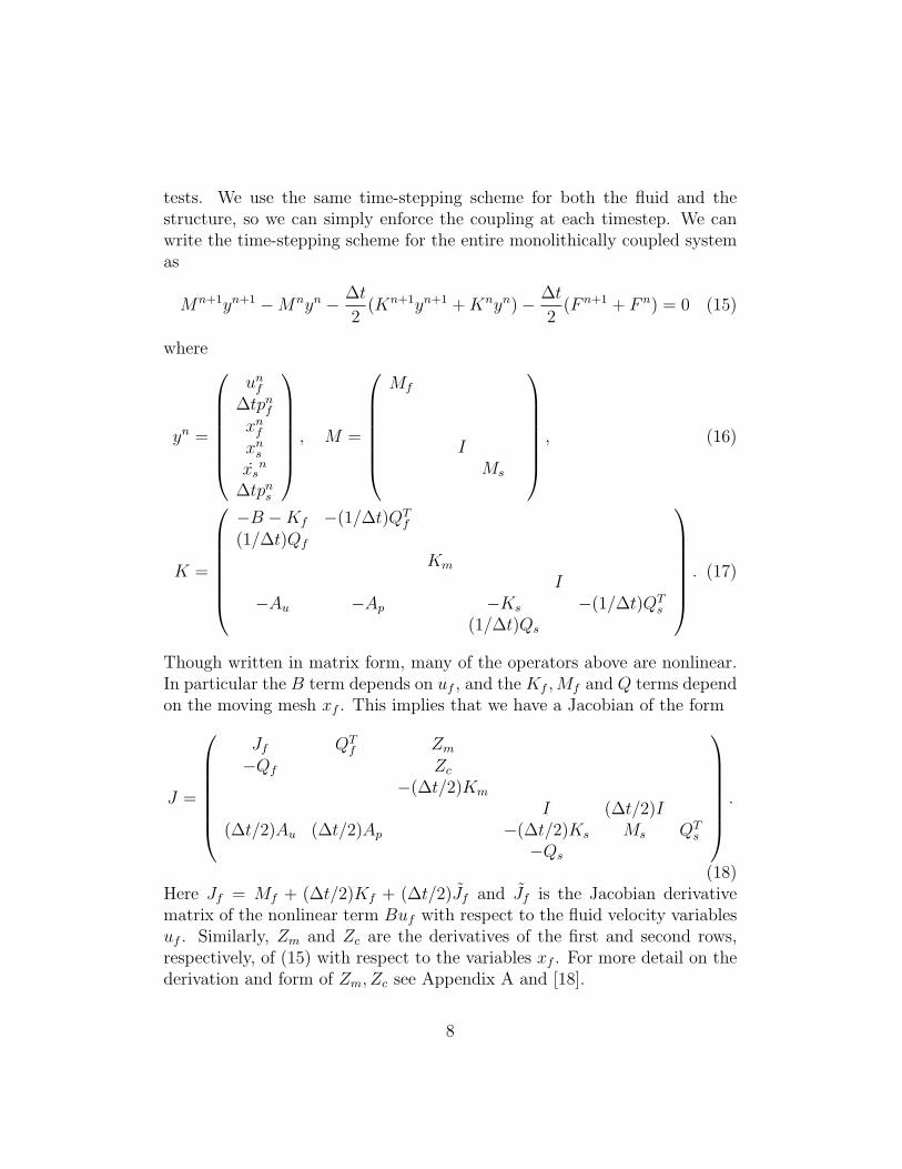
Figure 3: A portion of the branched geometry, shown with subdomains in different colorsand with structure elements darkened compared to fluid elements. Our algorithm doesdoes not notice the fluid-structure boundary in the partitions; that is, it sees the colorsbut not the shading.

For the sake of space in (18) we have not explicitly shown the couplingconditions (6) and (8). To show the coupled discretization of (6), for example,for only the uf and xs degrees of freedom, we can write

JΩf

f JΩfΓw

f

I −I

M Ωss M ΩsΓw

s

MΓwΩss MΓw

s

uΩf

f

uΓw

f

xsΩs

xsΓw

=

fΩf

f

0

f Ωss

fΓws

(19)

where the variables uf and xs have been split into portions on the fluid-structure interface Γw and portions on Ωf = Ωf\Γw and Ωs = Ωs\Γw respec-tively. The coupled discretization of (8) is similar.

This monolithically coupled nonlinear system is solved with a Newton-Krylov-Schwarz algorithm. It is this algorithm that forms the heart of thispaper and that we now go on to describe.

3. Scalable domain decomposition algorithms

At each time step, we solve the nonlinear system (15) with an inexactNewton method. At each Newton step we solve a preconditioned linearsystem of the form J(y)M−1(Ms) = z for the Newton correction s, where

9

M−1 is a one-level additive Schwarz preconditioner [38, 45]. The nonlinearsolver is an inexact Newton method with line search, and the linear system ateach Newton step is solved with restarted GMRES. For the nonlinear solver,we provide an exact hand-coded Jacobian that includes all the terms in (18),including the ones related to mesh movement, as in [18]. The nonlinear andlinear solvers are standard [38, 31], so we focus here on our construction ofthe preconditioner.

One of the underlying themes of this work is the tight, monolithic couplingof fluid and structure. This monolithic coupling extends all the way down tothe preconditioner; even the local solves within the Schwarz preconditionerinclude both fluid and structure elements, where a subdomain will typicallycontain both fluid and structure elements. See Figure 3.

To formally define the restricted additive Schwarz preconditioner M−1,we first partition the entire domain Ω into non-overlapping subdomainsΩℓ, ℓ = 1, . . . , N . This partition does not take into account the fluid-structureboundary. Then each subdomain Ωℓ is extended to overlap its neighbors,with the overlapping domains denoted Ω′

ℓ. The domain decomposition andextension respects element boundaries, so that each Ωℓ and Ω′

ℓ consists of anintegral number of finite elements. A parameter δ represents the size of theoverlap in terms of number of elements. Subdomains on a physical boundaryare not extended.

On each subdomain Ω′

ℓ we construct a subdomain preconditioner Bℓ,which is a restriction of the Jacobian matrix J , that is, it contains entriesfrom J corresponding to degrees of freedom contained in the correspond-ing subdomain Ω′

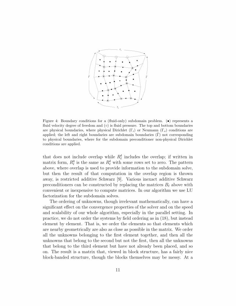
ℓ. Homogeneous Dirichlet boundary conditions are used onthe subdomain boundaries Γ for all solution variables, including fluid andstructure pressure; see Figure 4. For the Navier-Stokes equations this is notan appropriate boundary condition in theory; however, in practice it worksquite well. We emphasize that this boundary condition choice only affectsthe preconditioner on local subdomains. For the global solver, appropriatephysical boundaries conditions are applied on all boundaries.

The restricted additive Schwarz preconditioner can be written as

M−1 = (R01)

T B−11 Rδ

1 + · · · + (R0N)T B−1

N RδN . (20)

If n is the total number of unknowns in Ω and n′

ℓ is the number of unknownsin Ω′

ℓ, then Rℓ is an n′

ℓ×n restriction matrix which maps the global vector ofunknowns to those belonging to a subdomain. In particular R0

ℓ is a restriction

10

Γ ∼

Γ ∼

Γi

Γo

Figure 4: Boundary conditions for a (fluid-only) subdomain problem. (•) represents afluid velocity degree of freedom and () is fluid pressure. The top and bottom boundariesare physical boundaries, where physical Dirichlet (Γi) or Neumann (Γo) conditions areapplied; the left and right boundaries are subdomain boundaries (Γ) not correspondingto physical boundaries, where for the subdomain preconditioner non-physical Dirichletconditions are applied.

that does not include overlap while Rδℓ includes the overlap; if written in

matrix form, R0ℓ is the same as Rδ

ℓ with some rows set to zero. The patternabove, where overlap is used to provide information to the subdomain solve,but then the result of that computation in the overlap region is thrownaway, is restricted additive Schwarz [9]. Various inexact additive Schwarzpreconditioners can be constructed by replacing the matrices Bℓ above withconvenient or inexpensive to compute matrices. In our algorithm we use LUfactorization for the subdomain solves.

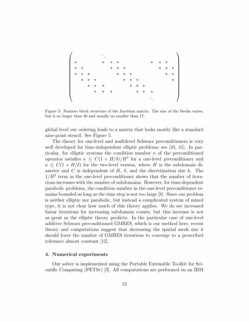
The ordering of unknowns, though irrelevant mathematically, can have asignificant effect on the convergence properties of the solver and on the speedand scalability of our whole algorithm, especially in the parallel setting. Inpractice, we do not order the systems by field ordering as in (18), but insteadelement by element. That is, we order the elements so that elements whichare nearby geometrically are also as close as possible in the matrix. We orderall the unknowns belonging to the first element together, and then all theunknowns that belong to the second but not the first, then all the unknownsthat belong to the third element but have not already been placed, and soon. The result is a matrix that, viewed in block structure, has a fairly niceblock-banded structure, though the blocks themselves may be messy. At a

11

. . .

∗ ∗ ∗ ∗ ∗ ∗ ∗∗ ∗ ∗ ∗ ∗ ∗ ∗ ∗∗ ∗ ∗ ∗ ∗ ∗ ∗ ∗

∗ ∗ ∗ ∗ ∗ ∗ ∗∗ ∗ ∗ ∗ ∗ ∗

∗ ∗ ∗ ∗ ∗ ∗. . .

Figure 5: Nonzero block structure of the Jacobian matrix. The size of the blocks varies,but is no larger than 40 and usually no smaller than 17.

global level our ordering leads to a matrix that looks mostly like a standardnine-point stencil. See Figure 5.

The theory for one-level and multilevel Schwarz preconditioners is verywell developed for time-independent elliptic problems; see [45, 41]. In par-ticular, for elliptic systems the condition number κ of the preconditionedoperator satisfies κ ≤ C(1 + H/δ)/H2 for a one-level preconditioner andκ ≤ C(1 + H/δ) for the two-level version, where H is the subdomain di-ameter and C is independent of H, δ, and the discretization size h. The1/H2 term in the one-level preconditioner shows that the number of itera-tions increases with the number of subdomains. However, for time-dependentparabolic problems, the condition number in the one-level preconditioner re-mains bounded as long as the time step is not too large [8]. Since our problemis neither elliptic nor parabolic, but instead a complicated system of mixedtype, it is not clear how much of this theory applies. We do see increasedlinear iterations for increasing subdomain counts, but this increase is notas great as the elliptic theory predicts. In the particular case of one-leveladditive Schwarz preconditioned GMRES, which is our method here, recenttheory and computations suggest that decreasing the spatial mesh size hshould leave the number of GMRES iterations to converge to a prescribedtolerance almost constant [12].

4. Numerical experiments

Our solver is implemented using the Portable Extensible Toolkit for Sci-entific Computing (PETSc) [3]. All computations are performed on an IBM

12

BlueGene/L supercomputer at the National Center for Atmospheric Researchwith 1024 compute nodes. Meshes are generated with Cubit from Sandia Na-tional Laboratory and partitioned with Parmetis [32, 39]. We validate thestructure part of the solver based on an analytic problem in [40] and thefluid problem part from [36]. The validation of the fluid-structure problemis discussed below.

4.1. Straight tube

Human artery walls are anisotropic in general, and because of the natureof pulsatile flow we can expect radial displacements to be larger than axialdisplacements. But there is no reason to believe that axial displacement isalways zero. We compare our numerical results with those in [2], where onlyradial displacement of the artery wall is considered, but our framework alsoallows for axial displacement. If both are included, the results are noticeablydifferent.

The setup of this test problem is a two-dimensional tube 6 cm by 1 cm,with walls at top and bottom of thickness 0.1 cm. A traction condition isapplied at the left boundary to induce a pressure pulse, which then travels tothe right, deforming the structure as it goes. In this example the kinematicviscosity νf = 0.0035 kg/m s, the Young’s modulus E = 7.5 · 104 kg/m s2,the structure is incompressible, and the inlet pressure pulse takes the form

σf · nf =−P0

2

[

1 − cos

(

πt

.0025s

)]

(21)

where P0 = 2.0 · 105 kg/m s2. We use γ = 4.0 · 109 kg/m3s2 and β = 0. Thetimestep size is ∆t = 0.0001 s, which is small because the timescale of thepressure pulse in (21) is shorter than the pulse produced by a physiologicalheartbeat. We fix the structure at the inlet and outlet (Γsd) with a zero dis-placement condition, and apply zero Neumann conditions to the structure atthe dry boundary Γsn. Neither of these conditions is physically very realistic,but they are commonly used in the literature [19]. A zero traction conditionis applied to the fluid at the outlet.

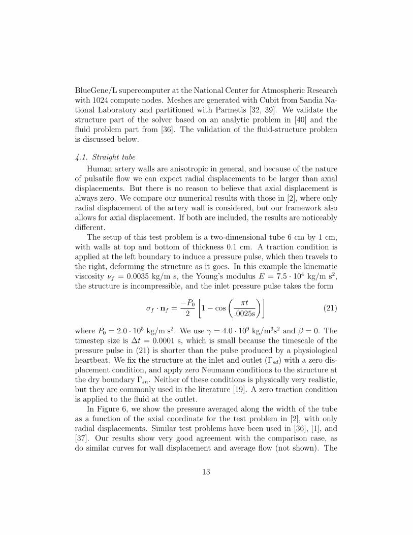
In Figure 6, we show the pressure averaged along the width of the tubeas a function of the axial coordinate for the test problem in [2], with onlyradial displacements. Similar test problems have been used in [36], [1], and[37]. Our results show very good agreement with the comparison case, asdo similar curves for wall displacement and average flow (not shown). The

13

0 1 2 3 4 5 6

0

5000

10000

15000

pre

ssure

(g /

cm

s2

)

t = 2.0 ms

0 1 2 3 4 5 6

0

5000

10000

15000

pre

ssure

(g /

cm

s2

)

t = 4.0 ms

0 1 2 3 4 5 6

0

5000

10000

15000

pre

ssure

(g /

cm

s2

)

t = 6.0 ms

0 1 2 3 4 5 6

0

5000

10000

15000

pre

ssure

(g /

cm

s2

)

t = 8.0 ms

0 1 2 3 4 5 6

0

5000

10000

pre

ssure

(g /

cm

s2

)

t = 10.0 ms

0 1 2 3 4 5 6

0

5000

10000

pre

ssure

(g /

cm

s2

)

t = 12.0 ms

Figure 6: Average pressure profiles for the test problem in [2] with only radial displace-ments allowed. The x-axis shows position, in cm, in the axial direction along the model.These results match the test problem very well.

14

0 1 2 3 4 5 6

0

5000

10000

15000pre

ssure

(g /

cm

s2

)

t = 2.0 ms

0 1 2 3 4 5 60

5000

10000

15000

pre

ssure

(g /

cm

s2

)

t = 4.0 ms

0 1 2 3 4 5 6

0

5000

10000

pre

ssure

(g /

cm

s2

)

t = 6.0 ms

0 1 2 3 4 5 6

0

5000

10000

pre

ssure

(g /

cm

s2

)

t = 8.0 ms

0 1 2 3 4 5 6

0

5000

10000

pre

ssure

(g /

cm

s2

)

t = 10.0 ms

0 1 2 3 4 5 6

0

5000

10000

pre

ssure

(g /

cm

s2

)

t = 12.0 ms

Figure 7: Average pressure profiles for the test problem in [2] with both radial and axialdisplacements. The x-axis shows position, in cm, in the axial direction along the model.

propagation of a pressure pulse is a key test for fluid-structure interaction,as it is completely dependent on the fluid-structure coupling; pressure moveswith infinite speed in an incompressible fluid with rigid walls.

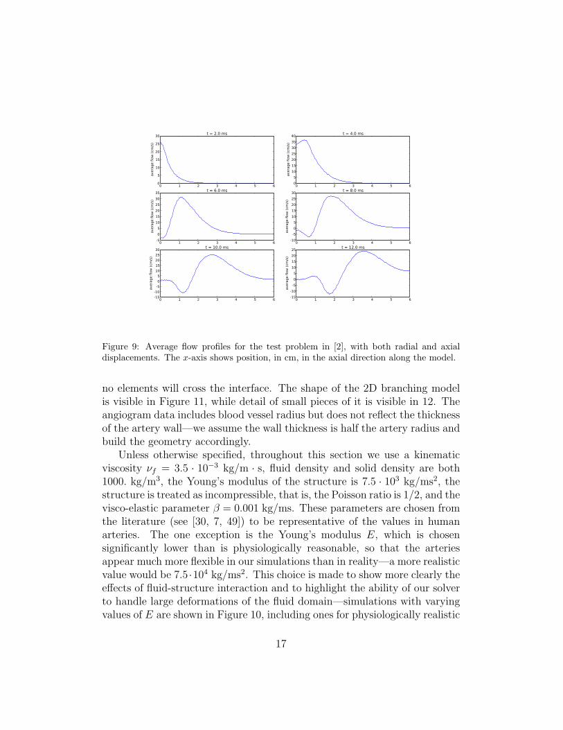
The results if we include axial displacement, on the other hand, are no-ticeably different; see Figures 7, 8, and 9. In particular, the pressure pulseis slightly slower, significantly more spread out, and the dip that follows theinitial positive pressure pulse is much more pronounced when axial displace-ment is taken into consideration. Qualitatively similar features can be seenin the pulse profile as viewed in the displacement and average flow plots ascompared to those in [2].

4.2. Branching model

Here we perform simulations for a complex branching geometry derivedfrom clinical data. The model we use comes from biplane angiography datafrom a pulmonary artery, courtesy of the Children’s Hospital, Denver. Weproject the data to a 2D plane, smooth it, and construct an unstructuredquadrilateral mesh with the Cubit package from Sandia National Laboratory.The fluid-structure interface is specified, and this software guarantees that

15

0 1 2 3 4 5 61.000

1.005

1.010

1.015

1.020

1.025

1.030

1.035

dia

mete

r (c

m)

t = 2.0 ms

0 1 2 3 4 5 60.98

1.00

1.02

1.04

1.06

1.08

1.10

1.12

1.14

dia

mete

r (c

m)

t = 4.0 ms

0 1 2 3 4 5 60.98

1.00

1.02

1.04

1.06

1.08

1.10

dia

mete

r (c

m)

t = 6.0 ms

0 1 2 3 4 5 60.96

0.98

1.00

1.02

1.04

1.06

1.08

dia

mete

r (c

m)

t = 8.0 ms

0 1 2 3 4 5 60.94

0.96

0.98

1.00

1.02

1.04

1.06

1.08

dia

mete

r (c

m)

t = 10.0 ms

0 1 2 3 4 5 60.94

0.96

0.98

1.00

1.02

1.04

1.06

1.08

dia

mete

r (c

m)

t = 12.0 ms

Figure 8: Diameter of the deforming fluid domain for the test problem in [2], with bothradial and axial displacements. The x-axis shows position, in cm, in the axial directionalong the model.

16

0 1 2 3 4 5 60

5

10

15

20

25

30

avera

ge f

low

(cm

/s)

t = 2.0 ms

0 1 2 3 4 5 60

5

10

15

20

25

30

35

40

avera

ge f

low

(cm

/s)

t = 4.0 ms

0 1 2 3 4 5 6-5

0

5

10

15

20

25

30

35

avera

ge f

low

(cm

/s)

t = 6.0 ms

0 1 2 3 4 5 6-10

-5

0

5

10

15

20

25

30

avera

ge f

low

(cm

/s)

t = 8.0 ms

0 1 2 3 4 5 6-15

-10

-5

0

5

10

15

20

25

30

avera

ge f

low

(cm

/s)

t = 10.0 ms

0 1 2 3 4 5 6-15

-10

-5

0

5

10

15

20

25

avera

ge f

low

(cm

/s)

t = 12.0 ms

Figure 9: Average flow profiles for the test problem in [2], with both radial and axialdisplacements. The x-axis shows position, in cm, in the axial direction along the model.

no elements will cross the interface. The shape of the 2D branching modelis visible in Figure 11, while detail of small pieces of it is visible in 12. Theangiogram data includes blood vessel radius but does not reflect the thicknessof the artery wall—we assume the wall thickness is half the artery radius andbuild the geometry accordingly.

Unless otherwise specified, throughout this section we use a kinematicviscosity νf = 3.5 · 10−3 kg/m · s, fluid density and solid density are both1000. kg/m3, the Young’s modulus of the structure is 7.5 · 103 kg/ms2, thestructure is treated as incompressible, that is, the Poisson ratio is 1/2, and thevisco-elastic parameter β = 0.001 kg/ms. These parameters are chosen fromthe literature (see [30, 7, 49]) to be representative of the values in humanarteries. The one exception is the Young’s modulus E, which is chosensignificantly lower than is physiologically reasonable, so that the arteriesappear much more flexible in our simulations than in reality—a more realisticvalue would be 7.5 ·104 kg/ms2. This choice is made to show more clearly theeffects of fluid-structure interaction and to highlight the ability of our solverto handle large deformations of the fluid domain—simulations with varyingvalues of E are shown in Figure 10, including ones for physiologically realistic

17

Figure 10: The pressure pulse in the straight tube problem, at 10 ms, for various valuesof the Young’s modulus E. At top left, E = 7.5 · 103 kg/m · s2, at top right E =3.0 · 104 kg/m · s2, at bottom left E = 7.5 · 104 kg/m · s2 (the physiological value usedin [2]), and at bottom right E = 7.5 · 105 kg/m · s2, which was used in [30]. In all casesβ = 0.001 kg/m · s. These plots are to be compared to the bottom left plot in Figures 6and 7. The profiles are somewhat different for different E but are qualitatively similar.

18

Figure 11: Deformation of the computational domain at systole (left) and diastole (right).In both pictures the fluid is colored by the norm of velocity (red is high and blue is low)while the structure is colored by pressure (again, red is high and blue is low, but in thestructure intermediate values are magenta rather than green). This simulation has Young’smodulus E = 7.5 · 104 kg/ms2 and a sinusoidally pulsing inlet boundary condition.

value for E used in previous blood flow simulations [2] and [30]. Though theprofiles here are different from each other, they certainly show more similaritywith each other than with the rigid-walled case.

In all the numerical results in the remainder of this paper, unless oth-erwise specified, we use a time step ∆t = 0.005 s—for the parameters ofthis problem, this time step size resolves essentially the same dynamics astests with smaller discretization sizes. We stop the linear solver when thepreconditioned residual has decreased by a factor of 10−4, we stop the New-ton iteration when the nonlinear residual has decreased by a factor of 10−6,and GMRES is set to restart every 60 iterations. For all our simulations westart with zero initial conditions and impulsively apply a velocity boundarycondition at the vessel inlet, choosing this case because of the computationaldifficulty. Tests where the fluid is started from a steady-state rather thanimpulsively from rest show similar scaling and solver characteristics. For thescaling results we proceed 10 time steps, reporting average time and nonlin-ear iteration count per time step, and average GMRES iterations per Newton

19

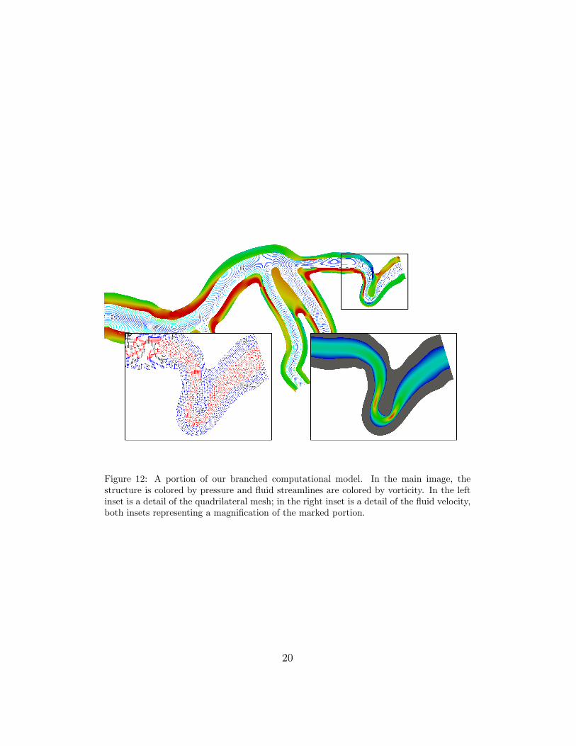
Figure 12: A portion of our branched computational model. In the main image, thestructure is colored by pressure and fluid streamlines are colored by vorticity. In the leftinset is a detail of the quadrilateral mesh; in the right inset is a detail of the fluid velocity,both insets representing a magnification of the marked portion.

20

32 64 128 256 512number of processors

1.0

1.5

2.0

2.5

3.0

3.5

4.0

speedup

8.33 ·105

1.63 ·106

2.40 ·106

3.67 ·106 ideal

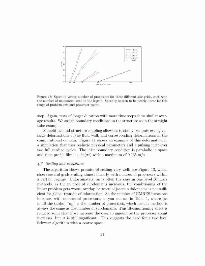
Figure 13: Speedup versus number of processors for three different size grids, each withthe number of unknowns listed in the legend. Speedup is seen to be nearly linear for thisrange of problem size and processor count.

step. Again, tests of longer duration with more time steps show similar aver-age results. We assign boundary conditions to the structure as in the straighttube example.

Monolithic fluid-structure coupling allows us to stably compute even givenlarge deformations of the fluid wall, and corresponding deformations in thecomputational domain. Figure 11 shows an example of this deformation ina simulation that uses realistic physical parameters and a pulsing inlet overtwo full cardiac cycles. The inlet boundary condition is parabolic in spaceand time profile like 1 + sin(πt) with a maximum of 0.165 m/s.

4.3. Scaling and robustness

The algorithm shows promise of scaling very well; see Figure 13, whichshows several grids scaling almost linearly with number of processors withina certain regime. Unfortunately, as is often the case in one level Schwarzmethods, as the number of subdomains increases, the conditioning of thelinear problem gets worse; overlap between adjacent subdomains is not suffi-cient for global transfer of information. So the number of GMRES iterationsincreases with number of processors, as you can see in Table 1, where (asin all the tables) “np” is the number of processors, which for our method isalways the same as the number of subdomains. This ill-conditioning effect isreduced somewhat if we increase the overlap amount as the processor countincreases, but it is still significant. This suggests the need for a two levelSchwarz algorithm with a coarse space.

21

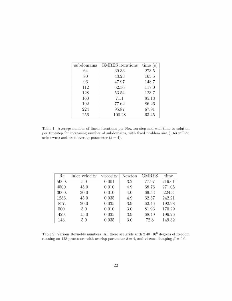
subdomains GMRES iterations time (s)64 39.33 273.580 43.23 165.596 47.97 148.7112 52.56 117.0128 53.54 123.7160 71.1 85.13192 77.62 86.26224 95.87 67.91256 100.28 63.45

Table 1: Average number of linear iterations per Newton step and wall time to solutionper timestep for increasing number of subdomains, with fixed problem size (1.63 millionunknowns) and fixed overlap parameter (δ = 4).

Re inlet velocity viscosity Newton GMRES time5000. 5.0 0.001 3.2 77.97 216.614500. 45.0 0.010 4.9 68.76 271.053000. 30.0 0.010 4.0 69.53 224.31286. 45.0 0.035 4.9 62.37 242.21857. 30.0 0.035 3.9 62.46 192.98500. 5.0 0.010 3.0 81.93 170.29429. 15.0 0.035 3.9 68.49 196.26143. 5.0 0.035 3.0 72.8 149.32

Table 2: Various Reynolds numbers. All these are grids with 2.40 · 106 degrees of freedomrunning on 128 processors with overlap parameter δ = 4, and viscous damping β = 0.0.

22

unknowns np ν Newton GMRES time8.33 · 105 128 0.4 3.9 37.62 41.728.33 · 105 128 0.45 3.9 40.08 42.068.33 · 105 128 0.5 3.9 43.97 40.691.63 · 106 256 0.4 3.6 57.58 62.131.63 · 106 256 0.45 3.6 63.97 64.431.63 · 106 256 0.5 3.6 72.22 64.582.40 · 106 512 0.4 3.5 93.4 70.882.40 · 106 512 0.45 3.4 99.88 70.342.40 · 106 512 0.5 3.4 115.29 73.49

Table 3: Tests for various values of the Poisson ratio ν. Higher Poisson ratio, even atthe incompressible limit, has only a modest effect on the behavior of the solver. Forbiological tissue, ν ≈ 0.5. In both the compressible and incompressible cases we use amixed formulation for elasticity.

The solver performs very well for a variety of Reynolds numbers. Thecompliant structure can absorb some energy from the fluid, so solving thefluid-structure problem for high Reynolds number is noticeably easier thanthe corresponding rigid-walled problem. Table 2 shows the performance ofthe solvers for different Reynolds number, as both inlet fluid velocity andfluid viscosity are varied.

The Poisson ratio ν is an important physical parameter for the solidmodel, with difficulty of simulation typically increasing as ν approaches theincompressible limit ν = 1/2. Biological tissue is nearly incompressible, so itis this limit that is of most interest in the simulation of blood flow. Bazilevset al. use a Poisson ratio of 0.4 in [7] and use 0.45 more recently in [6], butwith our mixed formulation for elasticity we have no difficulty going all theway to incompressibility, with ν = 0.5; see Table 3. Similarly, our solverworks well for a large range of ∆t; see Table 5.

Another important consideration in the design of fluid-structure inter-action algorithms is the added-mass effect, where solution becomes moredifficult if the density of the fluid and the structure are close to each other[10]. This problem mostly affects iterative coupling of fluid and structure,and our monolithic coupling seems to be immune to the added-mass effect;see Table 6.

In overlapping domain decomposition preconditioners like the one we use,

23

the overlap parameter δ plays a large role in the solution of the linear system.High δ corresponds to a stronger preconditioner and fewer iterations, but atthe cost of more global communication in the parallel algorithm. The effectsof various choices of δ can be seen in Table 4.

5. Conclusions and future work

Accurate modeling of blood flow in compliant arteries is a computationalchallenge. In order to meet this challenge, we need not only to model thephysics accurately but also to develop scalable algorithms for parallel com-puting. In this paper we have demonstrated a fluid-structure algorithm thatmonolithically couples fluid to structure, and is therefore quite robust tochanges in physical parameters and large deformation of the fluid domain.In addition, our solver features a Newton-Krylov-Schwarz method that scaleswell for large grids and large parallel machines, which represents a step for-ward in blood flow simulation.

In the future, more work is necessary to both improve physical realismand improve scalability. In particular, a coarse space in the Schwarz precon-ditioner is necessary to insure scalability to large numbers of processors. Forphysical realism, we need more physically meaningful outlet boundary con-ditions, a more sophisticated and complete structure model, and eventuallya three-dimensional method.

6. Acknowledgments

Special thanks to Feng-Nan Hwang, Yue Xue, and John Wilson for previ-ous work on this project and to Robin Shandas, Craig Lanning, and KendallHunter for help acquiring a patient-specific artery model. Thanks also toAlfio Quarteroni for discussions on the added mass effect and to GiovannaGuidoboni for discussions about the straight tube model problem.

References

[1] S. Badia, F. Nobile, and C. Vergara. Fluid-structure partitioned pro-cedures based on Robin transmission conditions. J. Comput. Phys.,227(14):7027–7051, 2008.

24

unknowns np overlap Newton GMRES time8.33 · 105 64 2 3.9 29.23 99.77*8.33 · 105 64 3 3.9 21.62 89.54*8.33 · 105 64 4 3.9 18.92 120.648.33 · 105 64 6 3.9 15.92 102.088.33 · 105 64 8 3.9 14.1 116.058.33 · 105 128 2 3.9 36.79 41.97*8.33 · 105 128 3 3.9 28.59 40.75*8.33 · 105 128 4 3.9 24.87 43.98.33 · 105 128 6 3.9 20.28 65.718.33 · 105 128 8 3.9 17.82 65.24*8.33 · 105 256 2 3.9 72.18 22.68*8.33 · 105 256 3 3.9 51.82 26.078.33 · 105 256 4 3.9 42.28 24.578.33 · 105 256 6 3.9 34.62 38.918.33 · 105 256 8 3.9 28.51 57.352.40 · 106 128 2 3.9 65.46 185.56*2.40 · 106 128 3 3.9 44.92 167.96*2.40 · 106 128 4 3.9 35.97 177.122.40 · 106 128 6 3.9 27.41 218.452.40 · 106 256 2 3.9 106.36 88.76*2.40 · 106 256 3 3.9 75.54 85.0*2.40 · 106 256 4 3.9 60.54 86.562.40 · 106 256 6 3.9 47.82 140.422.40 · 106 256 8 3.9 41.49 141.812.40 · 106 512 2 3.9 384.77 76.992.40 · 106 512 3 3.9 311.31 82.242.40 · 106 512 4 3.9 201.15 79.88*2.40 · 106 512 6 3.9 87.67 76.15*2.40 · 106 512 8 3.9 69.44 76.65

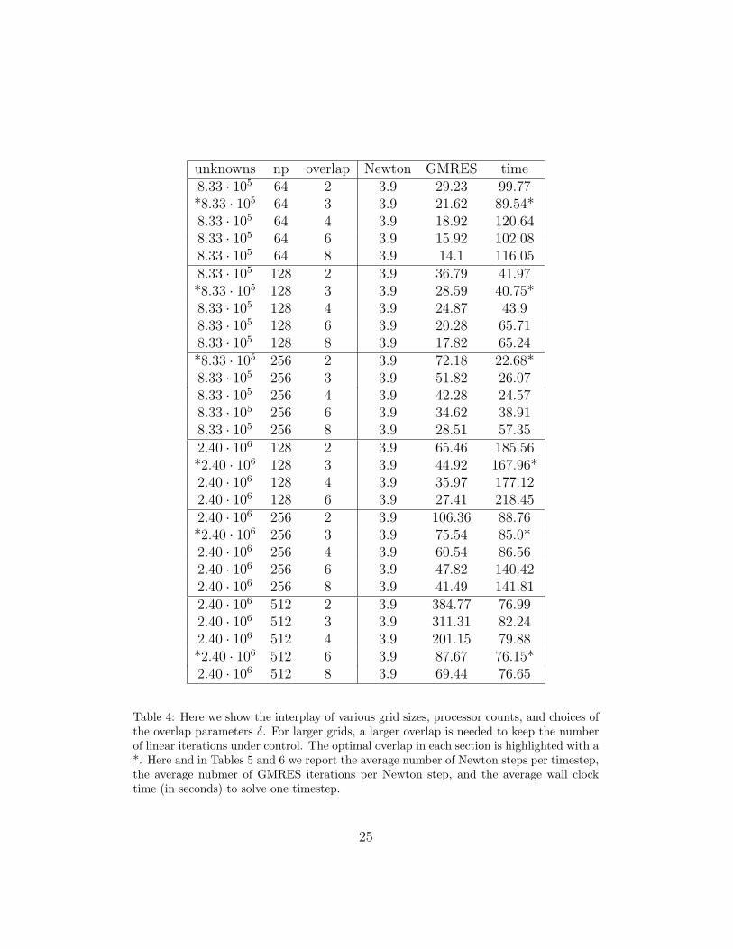
Table 4: Here we show the interplay of various grid sizes, processor counts, and choices ofthe overlap parameters δ. For larger grids, a larger overlap is needed to keep the numberof linear iterations under control. The optimal overlap in each section is highlighted with a*. Here and in Tables 5 and 6 we report the average number of Newton steps per timestep,the average nubmer of GMRES iterations per Newton step, and the average wall clocktime (in seconds) to solve one timestep.

25

unknowns np ∆t Newton GMRES time1.63 · 106 128 1.00 · 10−3 3.6 14.53 80.811.63 · 106 128 2.50 · 10−3 3.8 36.0 85.331.63 · 106 128 5.00 · 10−3 3.9 37.28 85.81.63 · 106 128 1.00 · 10−2 3.9 139.03 119.512.40 · 106 512 1.00 · 10−3 3.6 32.64 76.542.40 · 106 512 2.50 · 10−3 3.7 93.05 83.442.40 · 106 512 5.00 · 10−3 3.9 87.67 76.152.40 · 106 512 1.00 · 10−2 3.9 477.69 160.74

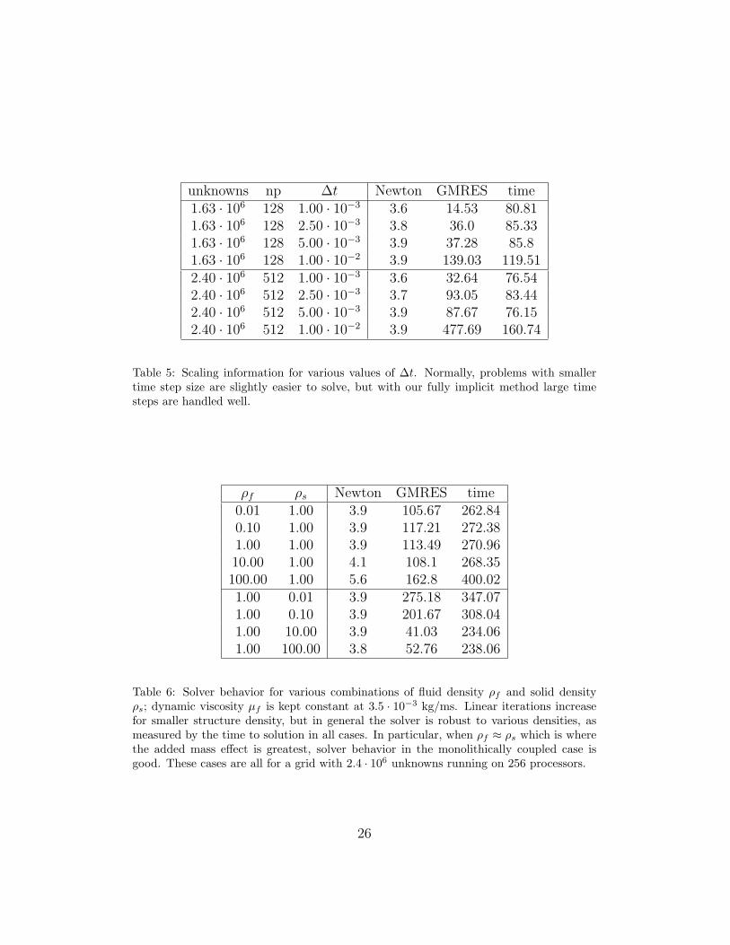
Table 5: Scaling information for various values of ∆t. Normally, problems with smallertime step size are slightly easier to solve, but with our fully implicit method large timesteps are handled well.

ρf ρs Newton GMRES time0.01 1.00 3.9 105.67 262.840.10 1.00 3.9 117.21 272.381.00 1.00 3.9 113.49 270.9610.00 1.00 4.1 108.1 268.35100.00 1.00 5.6 162.8 400.021.00 0.01 3.9 275.18 347.071.00 0.10 3.9 201.67 308.041.00 10.00 3.9 41.03 234.061.00 100.00 3.8 52.76 238.06

Table 6: Solver behavior for various combinations of fluid density ρf and solid densityρs; dynamic viscosity µf is kept constant at 3.5 · 10−3 kg/ms. Linear iterations increasefor smaller structure density, but in general the solver is robust to various densities, asmeasured by the time to solution in all cases. In particular, when ρf ≈ ρs which is wherethe added mass effect is greatest, solver behavior in the monolithically coupled case isgood. These cases are all for a grid with 2.4 · 106 unknowns running on 256 processors.

26

[2] S. Badia, A. Quaini, and A. Quarteroni. Splitting methods based on al-gebraic factorization for fluid-structure interaction. SIAM J. Sci. Com-

put., 30(4):1778–1805, 2008.

[3] S. Balay, K. Buschelman, V. Eijkhout, W. D. Gropp, D. Kaushik, M. G.Knepley, L. C. McInnes, B. F. Smith, and H. Zhang. PETSc usersmanual. Technical report, Argonne National Laboratory, 2008.

[4] A. T. Barker. Monolithic fluid-structure interaction algorithms for par-

allel computing with application to blood flow. PhD thesis, University ofColorado, Boulder, May 2009.

[5] Y. Bazilevs, V. Calo, J. Cottrell, T. Hughes, A. Reali, and G. Scovazzi.Variational multiscale residual-based turbulence modeling for large eddysimulation of incompressible flows. Comput. Methods Appl. Mech. En-

grg., 197:173–201, 2007.

[6] Y. Bazilevs, V. Calo, T. Hughes, and Y. Zhang. Isogeometric fluid-structure interaction: Theory, algorithms and computations. Comput.

Mech., pages 3–27, 2008.

[7] Y. Bazilevs, V. Calo, Y. Zhang, and T. Hughes. Isogeometric fluid-structure interaction analysis with applications to arterial blood flow.Comput. Mech., 38:310–322, 2006.

[8] X.-C. Cai. Additive Schwarz algorithms for parabolic convection-diffusion equations. Numer. Math., 60:42–62, 1990.

[9] X.-C. Cai and M. Sarkis. A restricted additive schwarz preconditionerfor general sparse linear systems. SIAM J. Sci. Comput., 21:792–797,1999.

[10] P. Causin, J. F. Gerbeau, and F. Nobile. Added-mass effect in the designof partitioned algorithms for fluid-structure problems. Comput. Methods

Appl. Mech. Engrg., 194(42-44):4506–4527, 2005.

[11] J. Donea, A. Huerta, J.-P. Ponthot, and A. Rodrıguez-Ferran. Arbi-trary Lagrangian-Eulerian methods. In E. Stein, R. de Borst, and T. J.Hughes, editors, Encyclopedia of Computational Mechanics, volume 1,pages 1–25. Wiley, 2004.

27

[12] X. Du and D. B. Szyld. A note on the mesh independence of convergencebounds for additive Schwarz preconditioned GMRES. Numer. Linear

Algebra Appl., 15:547–557, 2008.

[13] C. Farhat. CFD on moving grids: from theory to realistic flutter, ma-neuvering, and multidisciplinary optimization. Int. J. Comput. Fluid

Dyn., pages 595–603, 2005.

[14] C. Farhat and P. Geuzaine. Design and analysis of robust ALE time-integrators for the solution of unsteady flow problems on moving grids.Comput. Methods Appl. Mech. Engrg., 193(39-41):4073–4095, 2004.

[15] C. Farhat, P. Geuzaine, and C. Grandmont. The discrete geometric con-servation law and the nonlinear stability of ALE schemes for the solutionof flow problems on moving grids. J. Comput. Phys., 174(2):669–694,2001.

[16] C. Farhat, M. Lesoinne, and N. Maman. Mixed explicit/implicit timeintegration of coupled aeroelastic problems: three-field formulation, geo-metric conservation and distributed solution. Internat. J. Numer. Meth-

ods Fluids, 21(10):807–835, 1995. Finite element methods in large-scalecomputational fluid dynamics (Tokyo, 1994).

[17] L. Fatone, P. Gervasio, and A. Quarteroni. Multimodels for incompress-ible flows. J. Math. Fluid Mech., 2(2):126–150, 2000.

[18] M. A. Fernandez and M. Moubachir. A Newton method using exactjacobians for solving fluid-structure coupling. Comput. Struct., 83:127–142, 2005.

[19] C. A. Figueroa, I. E. Vignon-Clementel, K. E. Jansen, T. J. R. Hughes,and C. A. Taylor. A coupled momentum method for modeling bloodflow in three-dimensional deformable arteries. Comput. Methods Appl.

Mech. Engrg., 195(41-43):5685–5706, 2006.

[20] L. Formaggia, J. F. Gerbeau, F. Nobile, and A. Quarteroni. On thecoupling of 3D and 1D Navier-Stokes equations for flow problems incompliant vessels. Comput. Methods Appl. Mech. Engrg., 191(6-7):561–582, 2001.

28

[21] B. Fornberg. On the instability of leap-frog and Crank-Nicolson ap-proximations of a nonlinear partial differential equation. Math. Comp.,27:45–57, 1973.

[22] L. Grinberg and G. E. Karniadakis. A scalable domain decompositionmethod for ultra-parallel arterial flow simulations. Commun. Comput.

Phys., 4:1151–1169, 2008.

[23] M. Heil. An efficient solver for the fully coupled solution of large-displacement fluid-structure interaction problems. Comput. Methods

Appl. Mech. Engrg., 193(1-2):1–23, 2004.

[24] J. J. Heys, E. Lee, T. A. Manteuffel, and S. F. McCormick. On mass-conserving least-squares methods. SIAM J. Sci. Comput., 28(5):1675–1693 (electronic), 2006.

[25] J. J. Heys, T. A. Manteuffel, S. F. McCormick, and J. W. Ruge. First-order system least squares (FOSLS) for coupled fluid-elastic problems.J. Comput. Phys., 195(2):560–575, 2004.

[26] G. A. Holzapfel, T. C. Gasser, and R. W. Ogden. A new constitu-tive framework for arterial wall mechanics and a comparative study ofmaterial models. J. Elasticity, 61(1-3):1–48 (2001), 2000. Soft tissuemechanics.

[27] J. Hron and M. Madlık. Fluid-structure interaction with applications inbiomechanics. Nonlinear Anal. Real World Appl., 8(5):1431–1458, 2007.

[28] B. Hubner, E. Walhron, and D. Dinkler. A monolithic approach to fluid-structure interaction using space-time finite elements. Comput. Methods

Appl. Mech. Engrg., 193:2087–2104, 2004.

[29] T. J. Hughes. The Finite Element Method: linear static and dynamic

finite element analysis. Dover, 2000.

[30] K. S. Hunter, C. J. Lanning, S.-Y. J. Chen, Y. Zhang, R. Garg, D. D.Ivy, and R. Shandas. Simulations of congenital septal defect closure andreactivity testing in patient-specific models of the pediatric pulmonaryvasculature: a 3D numerical study with fluid-structure interaction. J.

Biomech. Eng., 128:564–572, 2006.

29

[31] F.-N. Hwang and X.-C. Cai. A parallel nonlinear additive schwarz pre-conditioned inexact Newton algorithm for incompressible Navier-Stokesequations. J. Comput. Phys., 204:666–691, 2005.

[32] G. Karypis. Metis/Parmetis web page, University of Minnesota, 2008.http://glaros.dtc.umn.edu/gkhome/views/metis.

[33] E. Kuhl, S. Hulshoff, and R. de Borst. An arbitrary Lagrangian Eulerianfinite-element approach for fluid-structure interaction phenomena. Int.

J. Numer. Methods Eng., 57:117–142, 2003.

[34] X. Ma, G. Lee, and S. Wu. Numerical simulation for the propagation ofnonlinear pulsatile waves in arteries. Trans. ASME, 114:490–496, 1992.

[35] C. J. Murray and A. D. Lopez. Mortality by cause for eight regionsof the world: Global Burden of Disease study. Lancet, 349:1269–1276,1997.

[36] F. Nobile. Numerical approximation of fluid-structure interaction prob-

lems with application to haemodynamics. PhD thesis, Ecole Polytech-nique Federale de Lausanne, 2001.

[37] F. Nobile and C. Vergara. An effective fluid-structure interaction for-mulation for vascular dynamics by generalized Robin conditions. SIAM

J. Sci. Comput., 30(2):731–763, 2008.

[38] S. Ovtchinnikov, F. Dobrian, X.-C. Cai, and D. E. Keyes. AdditiveSchwarz-based fully coupled implicit methods for resistive Hall magne-tohydrodynamic problems. J. Comput. Phys., 225(2):1919–1936, 2007.

[39] S. J. Owen and J. F. Shepherd. Cubit project web page, 2008.http://cubit.sandia.gov/.

[40] L. F. Pavarino and E. Zampieri. Overlapping Schwarz and spectralelement methods for linear elasticity and elastic waves. J. Sci. Comput.,27(1-3):51–73, 2006.

[41] B. Smith, P. Bjørstad, and W. Gropp. Domain Decomposition. Cam-bridge, 1996.

30

[42] D. Tang, C. Yang, H. Walker, S. Kobayashi, and D. N. Ku. Simulatingcyclic artery compression using a 3D unsteady model with fluid-structureinteractions. Comput. Struct., 80:1651–1665, 2002.

[43] C. A. Taylor and M. T. Draney. Experimental and computational meth-ods in cardiovascular fluid mechanics. Ann. Rev. Fluid Mech., 36:197–231, 2004.

[44] R. Torii, M. Oshima, T. Kobayashi, K. Takagi, and T. E. Tezduyar.Influence of wall elasticity in patient-specific hemodynamic simulations.Comput. Fluids, 36:160–168, 2007.

[45] A. Toselli and O. Widlund. Domain Decomposition Methods—

Algorithms and Theory. Springer-Verlag, Berlin, 2005.

[46] F. van de Vosse, J. D. Hart, C. V. Oijen, D. Bessems, T. Gunther,A. Segal, B. Wolters, J. Stijnen, and F. Baaijens. Finite-element-basedcomputational methods for cardiovascular fluid-structure interaction. J.

Engrg. Math., 47:335–368, 2003.

[47] I. E. Vignon-Clementel, C. A. Figueroa, K. E. Jansen, and C. A. Tay-lor. Outflow boundary conditions for three-dimensional finite elementmodeling of blood flow and pressure in arteries. Comput. Methods Appl.

Mech. Engrg., 195(29-32):3776–3796, 2006.

[48] X. Yue, F.-N. Hwang, R. Shandas, and X.-C. Cai. Simulation of branch-ing blood flows on parallel computers. Biomed. Sci. Instrum., 40:325–330, 2004.

[49] M. Zamir. The Physics of Pulsatile Flow. Springer, 2000.

[50] Y. Zhang, M. L. Dunn, E. Drexler, C. McCowan, A. Slifka, D. Ivy,and R. Shandas. A microstructural hyperelastic model of pulmonaryarteries under normo- and hypertensive conditions. Ann. Biomed. Eng.,33:1042–1052, 2005.

31

A. Jacobian construction

In this appendix we provide more details for the specific derivations of theterms in the Jacobian matrix J (18) for the nonlinear system (15). Providingan analytic hand-coded Jacobian can be very helpful for the efficiency andaccuracy of nonlinear solvers, but the actual construction of the Jacobian isoften a practical challenge.

A.1. The nonlinear function

Here we compute the term Jf from (18), that is, derivatives of the mo-mentum equations with respect to the fluid velocities uq, vq. This is the onlyterm of J that is also necessary in the case of an unmoving grid—most ofthe machinery in this appendix is for the moving grid case. The nonlinearconvective term B(u)u in the x direction is

∑

j

uj

∫

Ωt

∑

k

(

φ(x)k uk −

∂xk

∂tξ

(x)k

)

∂φ(x)j

∂xφ

(x)i +

∑

j

uj

∫

Ωt

∑

k

(

φ(y)k vk −

∂yk

∂tξ

(y)k

)

∂φ(x)j

∂yφ

(x)i (22)

where we have used φ to represent basis functions on the physical domainΩt in contrast to the reference domain Ω0—this distinction will become im-portant later. We have also written out completely the vector-valued basisfunctions φ

(x)k for clarity—there is a similar term involving the y direction

that is omitted above. Since in our implementation we use φk = ξk and∂xk/∂t = (xt

k − xt−1k )/∆t we can rewrite this as

∑

j

uj

∫

Ωt

∑

k

(

uk −xt

k − xt−1k

∆t

)

φ(x)k

∂φ(x)j

∂xφ

(x)i +

∑

j

uj

∫

Ωt

∑

k

(

vk −yt

k − yt−1k

∆t

)

φ(y)k

∂φ(x)j

∂yφ

(x)i . (23)

In this section of the appendix we are interested in derivatives of the aboveexpressions with respect to uq and vq, the velocity degrees of freedom.

32

Taking the derivative of (23) with respect to uq, we get

∑

j

uj

∫

Ωt

φ(x)i

∂φ(x)j

∂xφ(x)

q +∑

j

(

uj −xt

j − xt−1j

∆t

)

∫

Ωt

φ(x)i φ

(x)j

∂φ(x)q

∂x

+

∫

Ωt

∑

k

(

vk −yt

k − yt−1k

∆t

)

φ(x)i φ

(y)k

∂φ(x)q

∂y. (24)

And now taking the derivative with respect to vq we have

∑

j

uj

∫

Ωt

φ(x)i

∂φ(x)j

∂yφ(y)

q . (25)

The y direction equivalent of (22) behaves similarly, and this is how wecompute the term Jf in (18).

A.2. Dependence of the nonlinear function on the mesh

Here we are interested in derivatives of the momentum equations withrespect to the moving mesh, so we consider (23) with respect to xq and yq.As we will see, there are two dependencies here—one is explicit, because ofthe appearance of the mesh velocity in the advective term, and the otherappears because of the integration over a moving domain. We consider onlythe explicit nonlinear dependence in this section, and turn to the implicitdependence in A.3 and A.4. This provides one component of the Zm term in(18).

Taking the derivative of (23) with respect to xq we get

∑

j

uj

∫

Ωt

−1

∆tφ(x)

q

∂φ(x)j

∂xφ

(x)i . (26)

The y direction is similar.

A.3. Continuity equation

The momentum and continuity equations depend nonlinearly on the mov-ing mesh also because the integrals in the weak form of the equations aretaken over a moving domain, which depends on the mesh variables. Thisnonlinear dependence on the moving mesh is quite a bit more complex. Tounderstand it and show its form, we go in detail through the example of the

33

terms in Zc in (18), the dependence of the continuity equation on the movingmesh. In Section A.4 we will discuss how to generalize this to the terms inZm. The continuity equation in its discrete form is Qu = 0, and the Jacobianentries in Zc will take the form

Jik =∂

∂yk

∑

j

Qijuj =∑

j

uj

∂

∂yk

Qij (27)

with similar forms for the xk derivatives. Our finite element discretizationgives us

Qij =

∫

Ωt

ψi

∂φj

∂x(28)

for some of the entries, or a similar form with a derivative with respect to y.We want to calculate

∂

∂xk

Qij,∂

∂yk

Qij (29)

so as to compute (27). The first thing to notice is that the domain of in-tegration itself in (28) depends on the quantities xk, yk. To deal with this,we do what we do in practical implementations of the finite element methodanyway, and map the physical domain Ωt to a reference domain Ω0 = [−1, 1]2.

At this point we need to introduce some notation. The coordinates onthe physical domain are x, y and those on Ω0 are ξ, η. We will denote thefinite element basis functions on Ωt by φ and those on Ω0 by φ. We have themappings

x(ξ, η) =∑

s

φs(ξ, η)xs, y(ξ, η) =∑

s

φs(ξ, η)ys (30)

as interpolations based on the known mesh positions xs and ys. We do nothave easy access to the inverse mappings ξ(x, y), η(x, y), but we can stilltransform integrals from Ωt to Ω0 by

∫

Ωt

f(x, y) =

∫

Ωs

f(x(ξ, η), y(ξ, η))j (31)

where

j(ξ, η) =∂x

∂ξ

∂y

∂η−

∂x

∂η

∂y

∂ξ(32)

is the determinant of the Jacobian of the mapping (30)—we will call it theelement Jacobian in contrast to the nonlinear system Jacobian J .

34

We transform the integral in (28) to get

Qij =

∫

Ωt

ψi

∂φj

∂x=

∫

Ω0

ψi

∂φj

∂xj. (33)

Because of the finite element mapping (see for example [29]) we have

∂φj

∂x=

(

∂φj

∂ξ

∂y

∂η−

∂φj

∂η

∂y

∂ξ

)

/j. (34)

With this relation we can write

Qij =

∫

Ω0

ψi

(

∂φj

∂ξ

∂y

∂η−

∂φj

∂η

∂y

∂ξ

)

, (35)

and then using the interpolations (30) we have

∂y

∂η=

∑

s

∂φs

∂ηys (36)

and similarly for ∂y/∂ξ and similar terms involving the x mapping. In thisform we can take the kind of derivative we want, namely

∂

∂yk

∂y

∂η=

∂φk

∂η. (37)

Applying this to all the terms in (35), we get

∂

∂yk

Qij =

∫

Ω0

ψi

(

∂φj

∂ξ

∂φk

∂η−

∂φj

∂η

∂φk

∂ξ

)

(38)

which is an integral consisting only of quantities on the reference element—alldependence on x, y has been suppressed, and so this integral can be computedin the algorithm. Inserting this into (27), we can calculate the entries of theJacobian corresponding to the nonlinear effects of the moving mesh on thecontinuity equation—that is, we can fill in the entries of Zc in (18).

A.4. Other mesh dependence terms

The other mesh-dependence terms are derived similarly to those for thecontinuity equation. Each of the other terms forms a part of the term Zm

in (18), but the contributions for the mass matrix Mf , the viscosity matrix

35

Kf , the pressure term QTf , and the nonlinear term B are each calculated

separately and then added into the Zm block of the Jacobian.The general process is similar to that for the continuity equation—map

the integral to the reference domain, and then use (30), (32) and relationslike (34) to calculate derivatives with respect to xk, yk. In order to carry thisout, we need the corresponding y equation to (34), namely

∂φj

∂y=

(

−∂φj

∂ξ

∂x

∂η+

∂φj

∂η

∂x

∂ξ

)

/j. (39)

In the case of the continuity equation, two appearances of the element Ja-cobian j cancelled. In other cases we are not so lucky, so we may need thederivatives

∂

∂xk

j =∂φk

∂ξ

∑

s

∂φs

∂ηys −

∂φk

∂η

∑

s

∂φs

∂ξys (40)

∂

∂yk

j =∂φk

∂η

∑

s

∂φs

∂ξxs −

∂φk

∂ξ

∑

s

∂φs

∂ηxs. (41)

With these, using the product rule in combination with (34), (39) and (30),we can calculate derivatives with respect to xk, yk for any combinations ofbasis function derivatives. The resulting expressions can be quite complicatedto write down but the derivations are not difficult once we have the machineryabove.

36