Embed Size (px)
Citation preview
Scalable Self-Calibrating Display Technology for Seamless Large-Scale Displays
by
Rajeev J. Surati
S.M. Electrical Engineering and Computer Science Massachusetts Institute of Technology (1995)
S.B. Electrical Engineering and Computer Science Massachusetts Institute of Technology (1992)
Submitted to the Department of Electrical Engineering and Computer Science in Partial Fulfillment of the Requirements for the Degree of Doctor of Philosophy in Electrical
Engineering and Computer Science at the Massachusetts Institute of Technology
January 1999
Copyright Massachusetts Institute of Technology. All rights reserved.
Signature of Author______________________________________________________________ Department of Electrical Engineering and Computer Science
January 24, 1999
Certified by____________________________________________________________________ Thomas F. Knight Jr.
Senior Research Scientist Thesis Supervisor
Accepted by___________________________________________________________________ Arthur C. Smith
Chairman, Departmental Committee on Graduate Students

Scalable Self-Calibrating Technology for Seamless Large-Scale Displays
by
Rajeev J. Surati
Submitted to the Department of Electrical Engineering and Computer Science in Partial Fulfillment
of the Requirements for the Degree of Doctor of Philosophy in Electrical Engineering and
Computer Science at the Massachusetts Institute of Technology
Abstract We present techniques for combining high-performance computing with feedback to enable the correction of imperfections in the alignment, optical system, and fabrication of very high-resolution display devices. The key idea relies on the measurement of relative alignment, rotation, optical distortion, and intensity gradients of an aggregated set of low-cost image display devices using a precision low cost reference. Use of the reference allows the construction of a locally correct map relating the coordinate system of the aggregate display to the coordinate systems of the individual projectors composing the display. This idea provides a new technology for linearly scalable, bright, seamless, high-resolution large-scale self-calibrating displays (seamless video walls). Such a large-scale display was constructed using the techniques described in this dissertation. Low-cost computation coupled with feedback is used to provide the precision necessary to create these displays. Digital photogrammetry and digital image warping techniques are used to make a single seamless image appear across the aggregated projection displays. The following techniques are used to improve the display quality:
• Anti-alias filtering to improve the display of high frequency in images;
• Limiting the range of displayed intensities to ones that can be displayed uniformly across all the projectors; and
• Applying intensity smoothing functions to the regions of the image that are projected in the overlapping region. These functions smoothly and gradually transition the projection among the projectors.
The resultant systems demonstrate the viability of the approach by succeeding where other approaches have failed; it makes huge seamless video walls a reality.
Thesis Supervisor: Thomas F. Knight Jr. Title: Senior Research Scientist

Acknowledgements I would like to acknowledge the time, patience, and support given to me by my family: my wife,
Lisa, my parents Jay and Sudha, and my brother, Sanjeev.
Tom Knight, my thesis supervisor, is to be thanked for his brilliant ideas, inspiration, and for
understanding that founding a company is also a worthwhile endeavor.
Elmer Hung, although sometimes he is known as my arch-nemesis, inspired me to work harder
and better. I did enjoy the hack he and Luis played on me.
Luis Rodriguez has been a great person to bounce ideas off of and debate with. I thoroughly
enjoyed the evil hack I played on him.
Olin Shivers has always been there for me. Thanks for your confidence in me.
Hal Abelson and Gerry Sussman are to be thanked for fostering an environment at Project Mac
where students can easily pursue their independent interests. It was a wonderful place to work
with and meet people over the last 10 years including: Rebecca Bisbee, Daniel Coore, Natalya
Cohen, Peter Beebee, Andrew Berlin, Phillip Greenspun, Guillermo Rozas, Michael Blair,
Stephen Adams, Kleanthes Koniaris, Ron Weiss, Radhika Nagpal, Jacob Katznelson, Chris
Hanson, and Hardy Mayer.
The people at Flash Communications/Microsoft who had to endure my Ph.D. research.

4
Table of Contents
Abstract ................................................................................................................................................................ 2
Acknowledgements............................................................................................................................................... 3
Table of Contents ................................................................................................................................................. 4
Table of Figures.................................................................................................................................................... 6
Chapter 1 Introduction ........................................................................................................................................ 8
My Thesis ........................................................................................................................................................ 11
Solving the Problem ......................................................................................................................................... 12
System Architecture ......................................................................................................................................... 14
The Prototype System....................................................................................................................................... 14
Organization of Dissertation ............................................................................................................................. 15
Chapter 2 Background....................................................................................................................................... 17
Visual Perception ............................................................................................................................................. 17
Discrete Tiling of Video Cubes: The State of The Art ....................................................................................... 20
Calibrating Edge-Blended Projector Arrays to Display Seamless Images ........................................................... 21
Digital Photogrammetry ................................................................................................................................... 27
Digital Image Warping ..................................................................................................................................... 35
Conclusion ....................................................................................................................................................... 40
Chapter 3 Establishing the Positional Mappings............................................................................................... 41
Sub-pixel Registration ...................................................................................................................................... 41
Total Geometric Correction .............................................................................................................................. 42
Conclusion ....................................................................................................................................................... 44
Chapter 4 Establishing a Color and Intensity Mapping.................................................................................... 45
What does it take to be seamless? ..................................................................................................................... 45
How can we establish the mapping with our system?......................................................................................... 45
Creating the Mapping ....................................................................................................................................... 50
Implementation Results: ................................................................................................................................... 51
Conclusion ....................................................................................................................................................... 52
Chapter 5 Using the Mappings: A Seamless Display......................................................................................... 54
Warping Style .................................................................................................................................................. 54

5
Resampling ...................................................................................................................................................... 54
Effective Resolution: What Resolution is the System?....................................................................................... 55
Conclusion ....................................................................................................................................................... 60
Chapter 6 Conclusions and Future Work.......................................................................................................... 61
Conclusions...................................................................................................................................................... 61
Future work...................................................................................................................................................... 64
Bibliography....................................................................................................................................................... 66

6
Table of Figures
Figure 1-1: NASDAQ Market Site, New York 100 40” Rear Projection Cubes........................................................ 8
Figure 1-2: An image of a video wall in a news room that shows how visually apparent the seams are. .................... 8
Figure 1-3: An image capturing an attempt to display a familiar Window’s NT Desktop across a 2x2 projector array
visually highlights the distortion compensation ............................................................................................... 9
Figure 1-4: Displaying a single seamless image across the same 2 by 2 projector array in the exact same physical
arrangement pictured above using purely digital distortion correction based on our computation coupled with
feedback scheme(image displayed on system of Chaco Canyon, Az. USA is courtesy of Phillip Greenspun,
http://photo.net/philg). .................................................................................................................................. 10
Figure 1-5: Schematic diagram of prototype system. ............................................................................................. 12
Figure 1-6: Functional relationships between camera, projector, and screen space ................................................. 13
Figure 1-7: System architecture ............................................................................................................................ 14
Figure 1-8: Side view of prototype System............................................................................................................ 15
Figure 1-9: Front view of prototype system........................................................................................................... 16
Figure 2-1: Contrast sensitivity of the human eye as a function of field brightness. The smallest perceptible
difference in brightness between two adjacent fields ( ∆B ) as a fraction of the field brightness remains relatively
constant for brightness above 1 millilambert if the field is large. The dashed line indicates the contrast
sensitivity for a dark surrounded field[Smith 90]. .......................................................................................... 17
Figure 2-2: Spectral responsivities of the three types of photoreceptors in the human color vision system [Robertson
92] ............................................................................................................................................................... 18
Figure 2-3 Typical smoothing functions................................................................................................................ 23
Figure 2-4: Picture illustrating the difference in viewpoints from points A and B of two illuminated points on a high
gain screen (non-lambertian surface). The radius of each lobe emanating from the intersections of the lines
from viewpoints A and B represents the intensity as a function of viewed angle from a single screen location.26
Figure 2-5: Picture illustrating the difference in viewpoints from points A and B of two illuminated points on a 1.0
gain screen (lambertion surface). The radius of each lobe emanating from the intersections of the lines from
viewpoints A and B represents the intensity as a function of viewed angle from a single screen location. ....... 26
Figure 2-6: Picture of an extremely high gain screen while four LCD projectors are attempting to project black input
images. Because of the extremely high gain, the resultant image is an almost perfect reflection of the projectors,
thus the four bright spots. Thus the origin of hot spots is made more apparent................................................ 27
Figure 2-7 A picture of a calibration chart consisting of a regular two dimensional grid of squares. The effect of lens
distortion is grossly apparent in the image ..................................................................................................... 28
Figure 2-8: A sharply focused picture of a square in front of a CCD array. ............................................................ 32
Figure 2-9: Discretization of image with different kinds of values ......................................................................... 32
Figure 2-10: Figure illustrating the worst case error that can be induced with a partially covered pixel................... 33

7
Figure 2-11: The upper left hand corner of the black square surrounding the number character denotes the centroid
of the white square underneath it................................................................................................................... 34
Figure 2-12: Viking Lander picture of moon surface (distorted) ............................................................................ 35
Figure 2-13: Viking Lander picture of moon surface (undistorted)......................................................................... 35
Figure 2-14: Schematic diagram of input and outputs of a resampling system........................................................ 36
Figure 2-15: One-dimensional forward mapping ................................................................................................... 37
Figure 2-16: visual illustration of forward mapping............................................................................................... 38
Figure 2-17: One-dimensional inverse mapping .................................................................................................... 39
Figure 3-1: Image of test chart projected to determine camera to screen space mappings........................................ 42
Figure 3-2: Picture of grid in four projector overlap region.................................................................................... 44
Figure 4-1: Model of effects of illumination.......................................................................................................... 47
Figure 4-2: Feedback system in process of iterating to correct intensities for displayin a uniform green across the
system. ......................................................................................................................................................... 49
Figure 4-3: Picture of a single projector displaying its portion of an image ............................................................ 50
Figure 4-4: Picture of system displaying all white. ................................................................................................ 52
Figure 4-5: Picture of system displaying all black ................................................................................................. 52
Figure 5-1: Nearest Neighbor resampling of sinusoid bitmap ................................................................................ 56
Figure 5-2: Bilinear Interpolation resampling of sinusoid bitmap........................................................................... 57
Figure 5-3: Perfect resampling of sinusoid bitmap................................................................................................. 57
Figure 5-4: Normal bitmap Displayed on System using nearest neighbor resampling. ............................................ 57
Figure 5-5: Normal bitmap displayed on system using linear interpolation resampling........................................... 58
Figure 5-6: Vertical MTF ..................................................................................................................................... 58
Figure 5-7: Horizontal MTF ................................................................................................................................. 59
Figure 5-8: Angled MTF ...................................................................................................................................... 59
Figure 6-1: Picture of Chaco Canyon displayed on distorted system ...................................................................... 63
Figure 6-2: Corrected picture of Chaco Canyon displayed on distorted system ...................................................... 63

8
Chapter 1 Introduction People love to observe pictures and images displayed all around them. The bigger, the
brighter, the higher resolution, and the more inexpensive these displays are the better. The future
promises digital cinema and immersive virtual reality systems that provide a realistic visual
experience. While the computational power necessary to make these systems is available, the
high-quality large-scale displays are not. Those that we see at the shopping mall, on the nightly
news or at the subway station are either too low-resolution or have visible seams. Figure 1-1 for
example, shows the NASDAQ financial market site with over 100 video cubes working together
to simulate a single large screen. The NASDAQ video system cost millions of dollars. At the
time that display was constructed, there was no technology to eliminate seams at a reasonable
cost. Figure 1-2 makes the seams separating the aggregated video cubes more apparent.
Figure 1-1: NASDAQ Market Site, New York 100 40” Rear Projection Cubes
Figure 1-2: An image of a video wall in a news room that shows how visually apparent the seams are.

9
This dissertation describes a low-cost scalable digital technology based on coupling computation
with feedback that enables the projection of a single seamless image using an array of projectors.
The gross distortions that must be corrected in projector arrays are made visually apparent in
Figure 1-3. This figure shows the result of trying to display a familiar Microsoft Windows NT
desktop across a two by two projector array without any consideration for either geometrical or
intensity distortions. Current approaches to calibration of seamless displays using overlapped
projector arrays require manual positioning of projectors to eliminate geometric distortion
followed by manual optical and electronic calibration to eliminate intensity and color distortions.
Due to the sensitivity of these systems calibration must be repeated periodically to compensate
for drift. Because of the high cost of labor and inherent limitations of human vision, the cost of
such calibration is prohibitive. The technique described in this dissertation uses computational
modeling coupled with feedback from optical sensors to determine the geometric and intensity
distortions precisely and digitally compensate for all such distortions. The result is a seamless
image projected across an array. Figure 1-4 shows an image of the projectors used in Figure 1-3
Figure 1-3: An image capturing an attempt to display a familiar Window’s NT Desktop across a 2x2 projector array visually highlights the distortion compensation
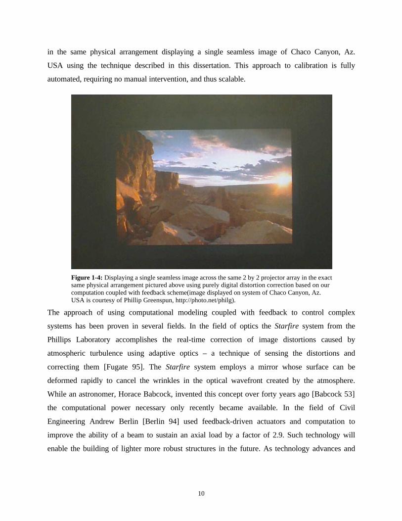
10
in the same physical arrangement displaying a single seamless image of Chaco Canyon, Az.
USA using the technique described in this dissertation. This approach to calibration is fully
automated, requiring no manual intervention, and thus scalable.
The approach of using computational modeling coupled with feedback to control complex
systems has been proven in several fields. In the field of optics the Starfire system from the
Phillips Laboratory accomplishes the real-time correction of image distortions caused by
atmospheric turbulence using adaptive optics – a technique of sensing the distortions and
correcting them [Fugate 95]. The Starfire system employs a mirror whose surface can be
deformed rapidly to cancel the wrinkles in the optical wavefront created by the atmosphere.
While an astronomer, Horace Babcock, invented this concept over forty years ago [Babcock 53]
the computational power necessary only recently became available. In the field of Civil
Engineering Andrew Berlin [Berlin 94] used feedback-driven actuators and computation to
improve the ability of a beam to sustain an axial load by a factor of 2.9. Such technology will
enable the building of lighter more robust structures in the future. As technology advances and
Figure 1-4: Displaying a single seamless image across the same 2 by 2 projector array in the exact same physical arrangement pictured above using purely digital distortion correction based on our computation coupled with feedback scheme(image displayed on system of Chaco Canyon, Az. USA is courtesy of Phillip Greenspun, http://photo.net/philg).
11
the cost of computation drops, computational modeling coupled with feedback will prove to be a
viable approach to solving a growing variety of problems.
My Thesis Low cost computation coupled with feedback can compensate for imperfections in the alignment, optical system and fabrication of very high-resolution composite display devices. Particularly, digital photogrammetry and digital image warping can be composed to computationally couple video feedback and projection. This entirely digital, scalable technology produces displays that are bright, high-resolution, portable and self-calibrating. This technology can create a single seamless wall using overlapping projected images. Furthermore, the purely digital approach enables the creation of display systems that can’t be engineered by conventional mechanical or optical means.
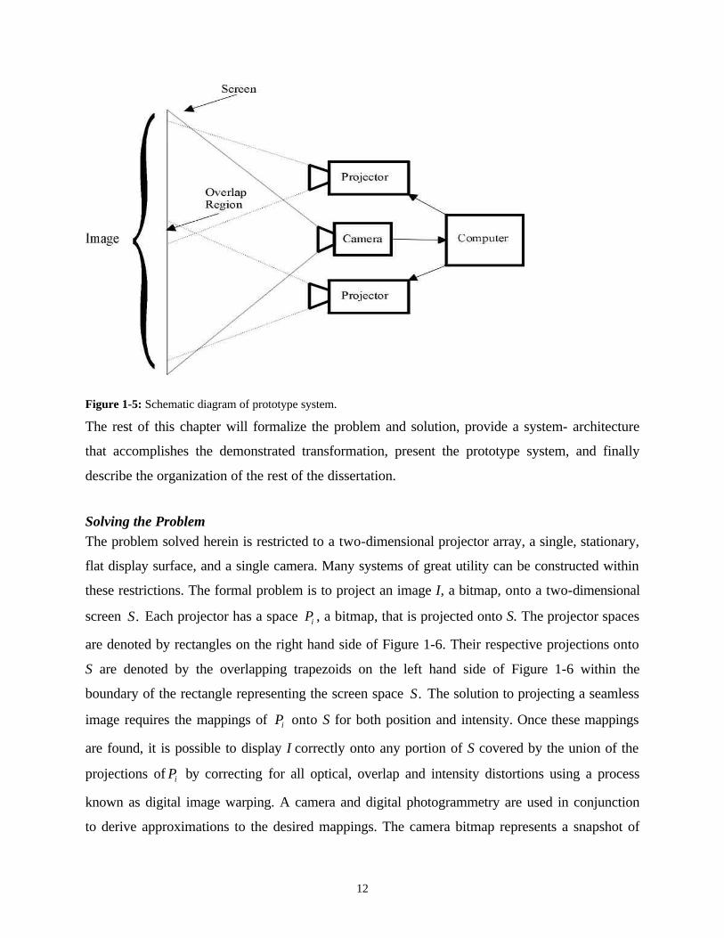
The viability of this thesis has been proven by the successful construction of a prototype system.
Figure 1-5 is a schematic diagram of the realized system. The camera provides the optical
feedback to the computer that is used in conjunction with digital photogrammetry techniques to
computationally compensate for the distortions visible in Figure 1-3. The geometric distortions
can be categorized as perspective distortions (resulting in the trapezoid shape of some of the
projections), pincushion and barrel distortions from the optics (resulting in the bowing outward
and inward of the projections), and alignment distortions between projectors (resulting in the
misalignment in the overlap region). Intensity and color distortions arise from using different
projectors with different light sources and optics, as well as having overlapping regions
illuminated by multiple projectors. The pre-distortions that are computed to compensate for these
distortions remap the position and intensity of each pixel to display a seamless image across the
system. The positional remapping enables the display of straight lines across the projection array
and limits the total displayed image to within the largest rectangular region that the array of
projected images covers. The intensity contribution of each pixel on a projector is modulated
such that when a uniform color and intensity bitmap is input into the frame buffer of the
computer, the image projected across the system will appear uniform for any particular
brightness level. Thus, pixels in different projectors whose projections overlap have their output
diminished such that the observed sum in the output achieves the seamless effect. Once these
pre-distortions are computed, the computer can apply digital image warping to the image in its
frame buffer and output appropriately pre-distorted projector input signals to display a seamless
representation of the image, as was done to generate Figure 1-4.
12
Figure 1-5: Schematic diagram of prototype system.
The rest of this chapter will formalize the problem and solution, provide a system- architecture
that accomplishes the demonstrated transformation, present the prototype system, and finally
describe the organization of the rest of the dissertation.
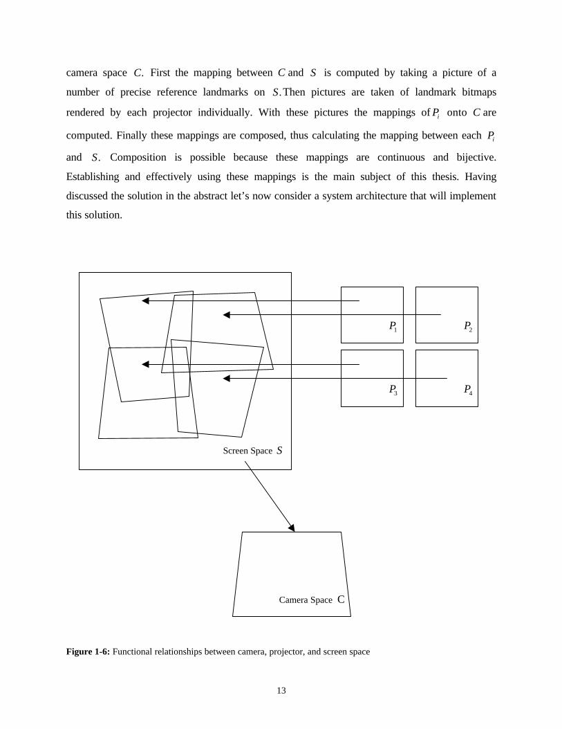
Solving the Problem The problem solved herein is restricted to a two-dimensional projector array, a single, stationary,
flat display surface, and a single camera. Many systems of great utility can be constructed within
these restrictions. The formal problem is to project an image I, a bitmap, onto a two-dimensional
screen .S Each projector has a space iP , a bitmap, that is projected onto S. The projector spaces
are denoted by rectangles on the right hand side of Figure 1-6. Their respective projections onto
S are denoted by the overlapping trapezoids on the left hand side of Figure 1-6 within the
boundary of the rectangle representing the screen space .S The solution to projecting a seamless
image requires the mappings of iP onto S for both position and intensity. Once these mappings
are found, it is possible to display I correctly onto any portion of S covered by the union of the
projections of iP by correcting for all optical, overlap and intensity distortions using a process
known as digital image warping. A camera and digital photogrammetry are used in conjunction
to derive approximations to the desired mappings. The camera bitmap represents a snapshot of
13
camera space .C First the mapping between C and S is computed by taking a picture of a
number of precise reference landmarks on .S Then pictures are taken of landmark bitmaps
rendered by each projector individually. With these pictures the mappings of iP onto C are
computed. Finally these mappings are composed, thus calculating the mapping between each iP
and .S Composition is possible because these mappings are continuous and bijective.
Establishing and effectively using these mappings is the main subject of this thesis. Having
discussed the solution in the abstract let’s now consider a system architecture that will implement
this solution.
Figure 1-6: Functional relationships between camera, projector, and screen space
Camera Space C
1P 2P
3P
Screen Space S
4P
14
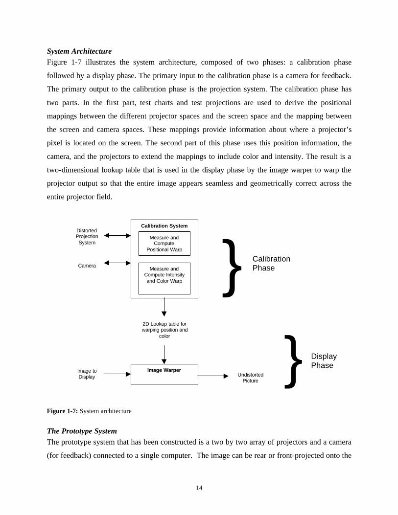
System Architecture Figure 1-7 illustrates the system architecture, composed of two phases: a calibration phase
followed by a display phase. The primary input to the calibration phase is a camera for feedback.
The primary output to the calibration phase is the projection system. The calibration phase has
two parts. In the first part, test charts and test projections are used to derive the positional
mappings between the different projector spaces and the screen space and the mapping between
the screen and camera spaces. These mappings provide information about where a projector’s
pixel is located on the screen. The second part of this phase uses this position information, the
camera, and the projectors to extend the mappings to include color and intensity. The result is a
two-dimensional lookup table that is used in the display phase by the image warper to warp the
projector output so that the entire image appears seamless and geometrically correct across the
entire projector field.
Figure 1-7: System architecture
The Prototype System The prototype system that has been constructed is a two by two array of projectors and a camera
(for feedback) connected to a single computer. The image can be rear or front-projected onto the
Distorted Projection System
Camera
Measure and Compute
Positional Warp
Measure and Compute Intensity and Color Warp
Calibration System
2D Lookup table for warping position and
color
Image Warper Image to Display Undistorted
Picture
} Calibration Phase
} Display Phase
15
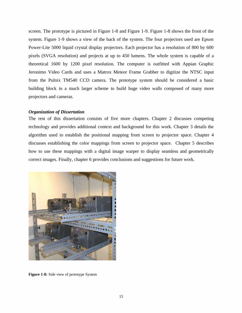
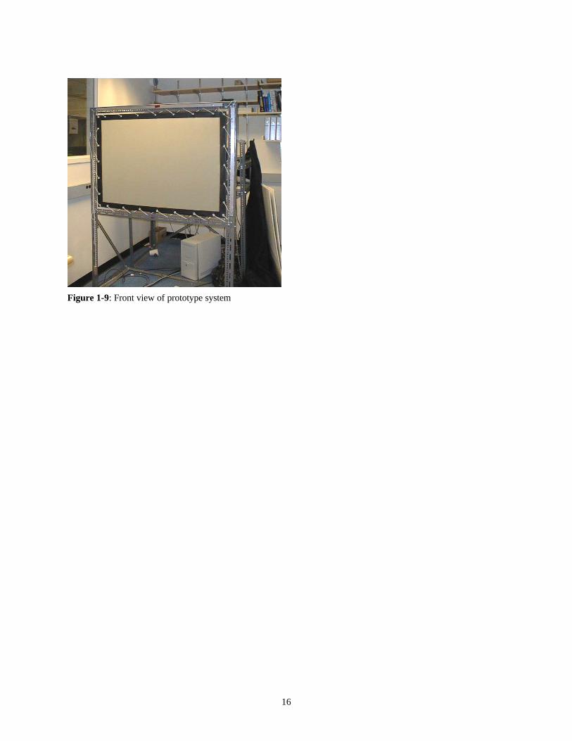
screen. The prototype is pictured in Figure 1-8 and Figure 1-9. Figure 1-8 shows the front of the
system. Figure 1-9 shows a view of the back of the system. The four projectors used are Epson
Power-Lite 5000 liquid crystal display projectors. Each projector has a resolution of 800 by 600
pixels (SVGA resolution) and projects at up to 450 lumens. The whole system is capable of a
theoretical 1600 by 1200 pixel resolution. The computer is outfitted with Appian Graphic
Jeronimo Video Cards and uses a Matrox Meteor Frame Grabber to digitize the NTSC input
from the Pulnix TM540 CCD camera. The prototype system should be considered a basic
building block in a much larger scheme to build huge video walls composed of many more
projectors and cameras.
Organization of Dissertation The rest of this dissertation consists of five more chapters. Chapter 2 discusses competing
technology and provides additional context and background for this work. Chapter 3 details the
algorithm used to establish the positional mapping from screen to projector space. Chapter 4
discusses establishing the color mappings from screen to projector space. Chapter 5 describes
how to use these mappings with a digital image warper to display seamless and geometrically
correct images. Finally, chapter 6 provides conclusions and suggestions for future work.
Figure 1-8: Side view of prototype System
16
Figure 1-9: Front view of prototype system

17
Chapter 2 Background This chapter begins by examining both the relevant principles of visual perception, by which the
quality of these displays must be evaluated, and the state-of-the-art in scalable technologies for
creating large-scale displays. The problems currently faced in calibrating edge-blended projector
arrays to produce seamless images are then discussed. Finally the basic techniques of digital
photogrammetry, and digital image warping used in this dissertation to automatically resolve
these issues are detailed.
Visual Perception A human vision system is the ultimate judge of whether or not we have successfully constructed
a seamless display. Unfortunately, we must rely on a combination of realizable sensors, such as
CCD imagers together with a detailed knowledge of human color perception. We must
understand the differences between a CCD imager and a pair of eyes. To that end, two areas of
visual perception important to our problem will be presented: uniformity of brightness, and color
reproduction and perception. [Tannas 92], [Wandell 95], [Thorell 90], [Smith 90] describe the
capabilities of the human eye in detail.
Figure 2-1: Contrast sensitivity of the human eye as a function of field brightness. The smallest perceptible difference in brightness between two adjacent fields ( ∆B ) as a fraction of the field brightness remains relatively constant for brightness above 1 millilambert if the field is large. The dashed line indicates the contrast sensitivity for a dark surrounded field[Smith 90].
18
Uniformity in Brightness
The eye isn’t a good judge of absolute brightness. It is however an extremely good instrument to
compare brightness. It can be used to match the brightness of two adjacent areas to an excellent
degree of precision. Figure 2-1 indicates the brightness differences that the eye can detect as a
function of the absolute brightness of the test areas being differentiated. At ordinary brightness
levels a difference greater than 2 percent is detectable. Contrast sensitivity is best when there is
no visible dividing line between two areas under comparison. When the areas are separated, or if
the demarcation between areas is not distinct, contrast sensitivity drops markedly.
Color Perception and Reproduction
In order to understand the physics of color reproduction, one must first understand the basics of
color perception. Even though the stimulus that enters our eyes and produces the perception can
be described and measured in physical terms, the actual color perceived is the result of a
complex series of processes in the human visual system. Below we will discuss the physics of
color receptors in the eye as well as higher level interactions that determine the perception of
colors. Some attention will be paid to how this understanding of color perception is used to
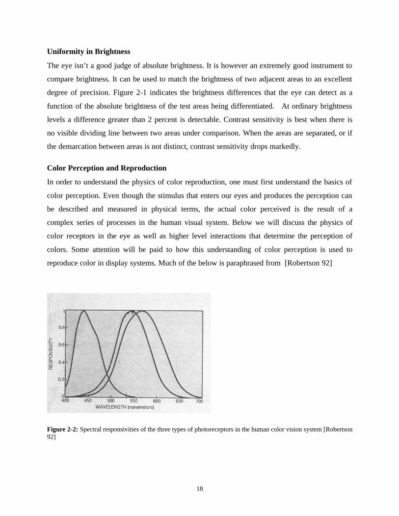
reproduce color in display systems. Much of the below is paraphrased from [Robertson 92]
Figure 2-2: Spectral responsivities of the three types of photoreceptors in the human color vision system [Robertson 92]
19
Physics of Color Receptors
When light enters the eye, it is focused onto the retina, absorbed by photoreceptors and
converted into neural signals. Three types of photoreceptors—known as cones because of their
shape—are sensitive to color. The rods, a fourth type of receptor are active at low light
levels(scotopic rather than photopic) but do not contribute to color vision. Each of the three types
of cones has a different type of spectral responsivity. Figure 2-2 shows the spectral responses for
each. Sometimes the types of cones are referred to as red, green and blue, but this is misleading
as the responses do not correspond to wavelengths that are usually perceived as having those
colors. Better terminology refers to them as long, medium and short-wavelength receptors.
The three responses have considerable overlap, a feature that is necessary to allow the visual
system to distinguish between light of different wavelengths. If for example, wavelengths in the
range 540-570 nm excited only one of the three cone types, the visual system could not
distinguish between intensity differences and wavelength differences in this range. In practice
wavelengths in that range excite long and middle-wavelength receptors, but the ratio of
responses varies with wavelength, allowing the observer to perceive a range of colors from green
to yellow.
A fundamental consequence of the existence of only three types of receptors is that many
different spectral radiance distributions can produce the same perceived color. For example, 6
watts of 540 nm radiation mixed with approximately 25 watts of 650 nm radiation will have the
same effect on the three receptors as 10 watts of 580 nm radiation. Spectral radiance distributions
that produce the same receptor response are known as metamers. Color reproduction systems
take advantage of metameric equivalence to accurately reproduce color psycho-physically. Thus
it is possible to create a tri-stimulus source that can span a large portion of the perceived visual
color range. [Smith 90] provides a detailed treatment explaining what colors are spanned by such
tri-stimulus sources. The most common set of additive sources used in this way have spectral
responses that are centered around red, green and blue. For maintaining color constancy, it is
clear that maintaining the relative contribution of each source at a point is extremely important.
Higher Level Processing
The prior discussion of colors dealt with the perception as if they occurred in isolation – as a
uniform field on a black background. While this is a good standard configuration for
20
fundamental studies of color, it hardly corresponds to the real world. The perceived color in self-
luminous systems is determined not only by the color stimulus to which it is directly associated,
but by neighboring stimuli in the field of view, and by other physical, physiological, and
psychological factors. One example showing the marked dependence of perceived color on the
surrounding stimuli is a stimulus that appears yellowish orange when seen in isolation. The same
stimulus will appear brown when seen against a much brighter white background. Other higher
level processing of neural inputs that affect perceived color is memory of customary appearance
of scenes and assumptions about the context in which stimuli are perceived. These higher level
effects are often not considered or modeled in the design of color reproduction systems.
Undoubtedly, a superior system would take these factors into account.
We have discussed and coarsely characterized the human visual perception to gain an
understanding of how to use a camera in our feedback system. From this description it is possible
to understand and evaluate the design decisions for uniformity of brightness and color
reproduction in our system. We now move on to discussing alternate technologies for large-scale
displays.
Discrete Tiling of Video Cubes: The State of The Art The current state of the art scalable projection systems ultize multiple projectors. Single projector
technology has failed to scale to large displays for three fundamental reasons: low fabrication
yield of high-resolution projection components, high power requirements, and geometric
constraints necessary to avoid large variations in optical path lengths resulting in uneven pixel
shape, size and power distribution. Discrete tiling of video cubes is a scalable technology that
addreses all of these issues. Rather than relying on a single projector, discrete tiling juxtaposes
single rear projection systems called video cubes to create display systems that scale linearly in
both resolution and brightness. The resultant systems are, however, marred by visible artifacts. A
screen four times larger with four times the resolution and the same brightness requires four
times as many projectors. Notably the optical path length does not change with the larger screen
requirement as it would if a single projector were used. By using existing commodity projection
display technology, one can at all times exploit the highest resolution technology available in
high yield and thus enjoy lower cost. The systems constructed, however, suffer from two
significant visible drawbacks. The first drawback is a visible mullion, the black area between

21
each projector's projected image. Typically the black area is between 8 and 50 mm wide. Despite
the small width of the mullion in the picture (8 mm), the seam is still quite noticeable. The
second drawback is that each of the projectors must be calibrated to uniformly display different
colors in unison. The discretely tiled systems pictured in Figure 1-1 and Figure 1-2 make these
drawbacks apparent. As noted before, the separation between cubes reduces the contrast
sensitivity of the eye across the seam. Thus the distinct separation makes it easier to calibrate
uniformity in brightness and color. Each particular projection technology has its own set of
problems that must be addressed to solve this uniform color and brightness problem. For CRT
based displays, one must first converge all the projection systems. Then it is possible to square
each projectors image to squarely join with the other images across the visible boundary. Finally
one must reduce the variances in colors across the monitors. The calibration described here must
be performed periodically because of analog drift. For example, the CRT based system pictured
in Figure 1-1 is calibrated once a month. This takes a total of sixteen man-days. For light-valve
systems, the problem is that the light sources degrade differently over time across projectors.
Thus, any correction done across the system must be redone at a later date depending on system
usage. If any bulb degrades significantly differently from the others, all the bulbs in the system
need to be replaced to make certain of uniformity in brightness across the system. While this
approach provides large-scale systems that scale in resolution and brightness, eliminating the
visible seam represents a substantial improvement.
Calibrating Edge-Blended Projector Arrays to Display Seamless Images In this section we examine the basic problems and issues encountered in calibrating edge-
blended projector arrays to display seamless images. [Lyon 86] and [Lyon 84] provide detailed
descriptions of all the issues and some applicable solutions, though these papers are written to
describe the problems faced in manually calibrating these systems. Below we will discuss those
issues relevant to our approach: registration accuracy in the overlap region, perceived color
match between adjacent projectors, intensity variation across the boundaries, brightness
uniformity across the entire viewing area, contrast ratios, white and black levels, and exit pupil
size. It is worth noting that because all geometric distortion correction is accomplished digitally
in our approach, it is not necessary to discuss the physical alignment of the projectors used to
22
eliminate geometric distortion in manually calibrated systems, an important issue discussed in
the aforementioned papers.
Registration Accuracy in Overlap Region
The major problem is attaining highly accurate pixel registration in the projected overlap. Such
registration creates the ability to draw straight lines across the overlap region from one projector
to the other. Lyon asserts that the registration accuracy in the overlap region should be as good as
that of any single independent projection channel. In practice this means that the registration
accuracy for the red, green and blue images projected by each projector must be comparable to
that achieved between different projector channels. A difference in accuracies between overlap
and non-overlap regions, is potentially noticeable, and thus could make a seam visible. The
registration accuracy for multiple gun or light-valve single projector systems is typically 1/4
pixel.
Perceived Color Match Between Adjacent Projectors
If the different projector colors don't match, attempting to display a uniform color across the
boundary will make the seam apparent. The input to adjacent projectors must be adjusted so that
the seam is not apparent when a uniform color is displayed across the overlap region. As
discussed in the visual perception section, the system must be adjusted so that the relative
contributions from each of the three types of color sources contributing to a pixel’s color are
matched across the system for any particular color displayed.
Intensity Variation Across Boundaries
An abrupt change in intensity or color from one channel to another in the overlap region is
unacceptable. As noted before, the contrast sensitivity of the eye is greatly reduced when the area
of overlap is not clearly demarcated. Thus, an easy way to make a uniformly perceived transition
is to apply smoothing functions to the input to each projector based on the position of an input
pixel in the projected image. If the pixel is in an overlap region, then that projector’s contribution
to the total output should be lowered the closer the pixel is to the projector’s projected image’s
edge. The other projectors must also similarly reduce their input. However, the net sum of their
contributions to the total brightness, must sum to one, to make it appear as if only one projector

23
was projecting into overlap. Care must be taken so that these smoothing function properly factor
in each projector's gamma correction for each color. Otherwise, the seams will appear as either
brighter or dimmer than the rest of the image. Figure 2-3 shows what these smoothing functions
often look like in one-dimension to make the concept easy to see. The two edge-blending
functions that have been created assume that the two projectors they apply to overlap
horizontally and that both their top and bottom edges perfectly overlap in the overlap region.
Each edge-blending function gradually transitions from one down to zero. Each projector's edge-
blending function will be multiplied with each input raster line. One can see that the edge-
blended functions pictured sum to one. That is what should happen with the projector's projected
images provided their corresponding raster lines are properly lined up in space. If everything is
aligned correctly, then the intensity of the overlap region summed from both projectors will look
as though it were generated by one projector. These smoothing functions must be manually
calibrated for each horizontal input line of each projector. Lyon's experiments suggest that for
every degree of channel overlap, a 2 percent variation in intensity, if smooth, is imperceivable.
Figure 2-3 Typical smoothing functions
Brightness Uniformity Across the Entire Viewing Area
Without brightness uniformity across the system, the edges of each projector's projected image
get accented and become conspicuous, revealing the seams. This effect can be compensated for
in the smoothing functions that are applied. In single projector systems there is a brightness
gradient from the center of the image to the edge typically caused by vignetting. The brightness
ratio from center to edge can be as high as 1.66. In rear-projection this effect coupled with
limited projection screen diffusion can cause hotspots. One way to reduce this problem for each
projector is to increase the f-number of the projector lenses. Fixing this problem for a single
Intensity Smoothing Functions
0
0.2
0.4
0.6
0.8
1
1.2
1
Horizontal Location
Right Projector
Left Projector
Sum of Left and Right Projectors

24
projector is difficult. Trying to do this among several projectors and deal with overlap regions is
even more difficult. Usually it is done in an extremely coarse manner. However, care must be
taken in getting the overlap region transitions to be smooth enough to eliminate the visible
seams. Smooth variation across the system is tolerable, as the wide angle of view affords larger
tolerances for uniform perception.
Contrast Ratios, White and Black Levels
The contrast ratio in a display system is the ratio between the brightest white (white level) and
the blackest black (black level). Typical cathode ray tubes achieve ratios above 30. The lowest
number, 30, is barely acceptable for a display as determined through perception experiments
[Projection Basics]. For projection displays, ratios higher than 80 are considered reasonable
[Projection Basics]. Notably the white level is determined by the minimum intensity displayed
when all the projectors are displaying their brightest white. The black-level in these systems is
determined by the brightest intensity displayed when all the projectors overlap and are
attempting to project black. Typically there are at most four projectors overlapping. It is possible
to limit that number to three. There is no disadvantage to doing this, though it is not the
convention in small-scale manually calibrated systems. Thus the contrast ratio is at worst
approximately four times the black level of a typical projector. This suggests the contrast ratio
would be at best one quarter the contrast ratio achievable by the dimmest projector in the array if
the black-level for each pixel were raised to the aforementioned maximum level. One can try to
mitigate this effect some by not overlapping all four projectors. At best, however, the contrast
ratio is three times worse than a single projector’s ratio with at most three overlapping projectors.
Brightening up the black level at any position on the screen can substantially lower the dynamic
range available to display pictures. This trade-off is too expensive and will result in poor image
quality. Thus, the strategy taken in these systems is to not raise the black level to the overlap
region black level. Rather the black level is kept where it is in order to preserve larger contrast
ratio. The cost is that when attempting to display black, the seams are visible. However, as the
ambient light rises to greater than the black level at the overlap, the seam becomes less apparent
and will not be visible when attempting to project black images. Its also worth perhaps looking at
the range of intensities in the image being display and using that to determining what contrast
ratio strategy is used to display each particular image.

25
Large Exit Pupil Size
The exit pupil is the envelope from which quality edge-blending can be viewed. The size of this
region is determined by how the projected light rays are absorbed, reflected and diffused by the
screen surface. If the image is viewed outside this eye envelope, a distinct brightness mismatch
becomes apparent across projection boundaries. This is a result of the screen surface reflecting or
transmitting perceivably unequal amounts of light toward the viewer from juxtaposed projectors.
Screen gain quantifies the dispersion of transmitted or reflected light for either a front-projection
or rear-projection screen. A screen with gain of 1.0, known as a lambertian screen, is one that
disperses light uniformly without regard to its incident angle. The higher a gain screen one uses,
the more the dispersion of light is affected by the angle of incidence of the source light.
To illustrate what screen gain means Figure 2-4 and Figure 2-5 contrast the two different
viewpoints A and B of two equally illuminated points on a high gain screen in Figure 2-4 and a
1.0 gain screen in Figure 2-5. The two lopsided lobes emanating from the screen indicate the
power viewed from that point as a function of angle. Thus the intersection of a line drawn from a
viewpoint with lobes emanating from the illuminated points gives a relative measure of the
difference in intensity viewed from either screen point. The two lobes emanating from the
screens indicate the power viewed of that point as a function of angle. Thus the intersection of a
line drawn from a viewpoint with the lobes emanating from the illuminated screen points gives a
relative measure of the difference in intensity viewed from either screen point. Hence, the left
point looks a lot brighter than the right point from viewpoint A in Figure 2-4. The left point and
right point look equally bright from viewpoint B in Figure 2-4. The left and right point look
equally bright from any viewpoint in Figure 2-5. Note this property is very desirable for our
purposes. The shape of the lobes in the pictures is indicative of the gain. The hemispheres are
associated with screens of gain 1.0. The more like tear drops the lobes become the higher the
gain. An impulse would be associated with total reflection (or transmission depending on the
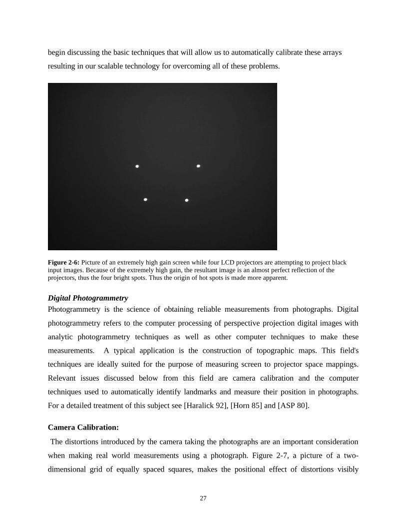
type of projection) or infinite gain. Figure 2-6 provides an illustration of such a screen. It is a
picture of a very high gain screen with four liquid crystal projectors attempting to display black
input images. LCD projectors try to display black by attempting to attenuate the transmission of
light through the liquid crystal. The resultant image shows the clear outline of the light
emanating from the projectors. These are what called hot spots. As the gain goes down there is
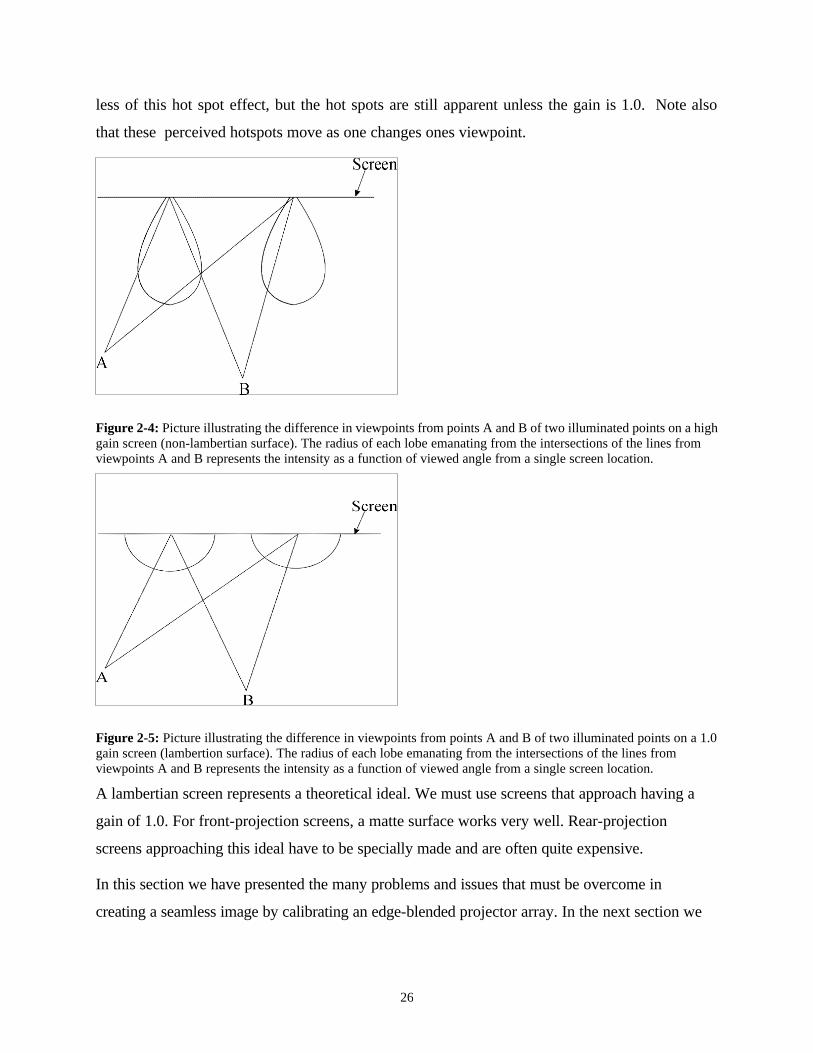
26
less of this hot spot effect, but the hot spots are still apparent unless the gain is 1.0. Note also
that these perceived hotspots move as one changes ones viewpoint.
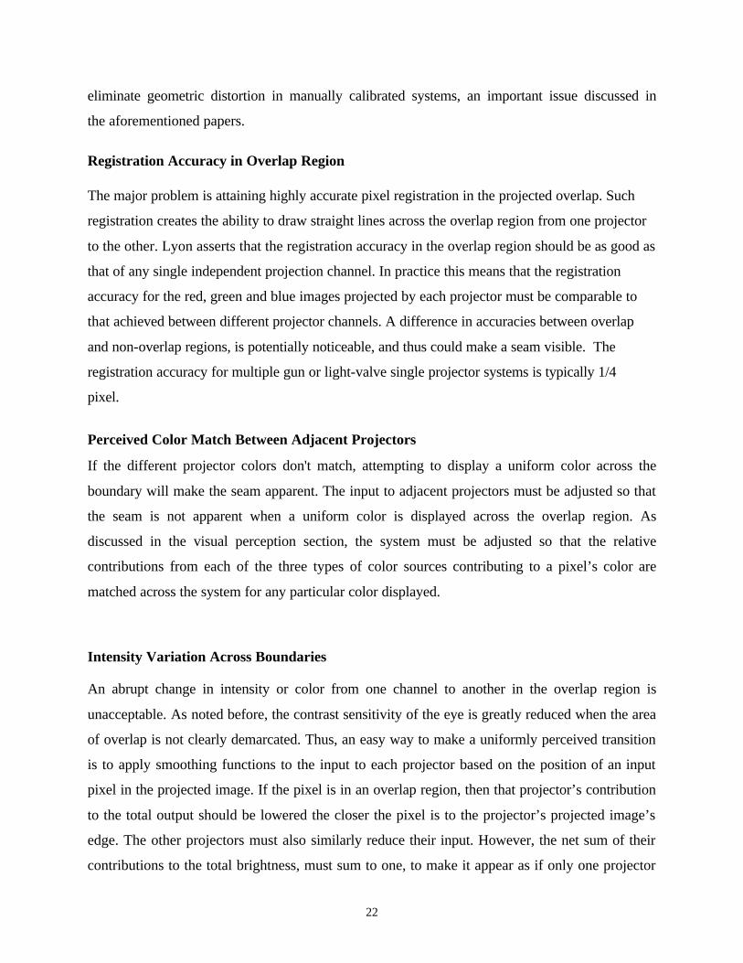
Figure 2-4: Picture illustrating the difference in viewpoints from points A and B of two illuminated points on a high gain screen (non-lambertian surface). The radius of each lobe emanating from the intersections of the lines from viewpoints A and B represents the intensity as a function of viewed angle from a single screen location.
Figure 2-5: Picture illustrating the difference in viewpoints from points A and B of two illuminated points on a 1.0 gain screen (lambertion surface). The radius of each lobe emanating from the intersections of the lines from viewpoints A and B represents the intensity as a function of viewed angle from a single screen location.
A lambertian screen represents a theoretical ideal. We must use screens that approach having a
gain of 1.0. For front-projection screens, a matte surface works very well. Rear-projection
screens approaching this ideal have to be specially made and are often quite expensive.
In this section we have presented the many problems and issues that must be overcome in
creating a seamless image by calibrating an edge-blended projector array. In the next section we
27
begin discussing the basic techniques that will allow us to automatically calibrate these arrays
resulting in our scalable technology for overcoming all of these problems.
Figure 2-6: Picture of an extremely high gain screen while four LCD projectors are attempting to project black input images. Because of the extremely high gain, the resultant image is an almost perfect reflection of the projectors, thus the four bright spots. Thus the origin of hot spots is made more apparent.
Digital Photogrammetry Photogrammetry is the science of obtaining reliable measurements from photographs. Digital
photogrammetry refers to the computer processing of perspective projection digital images with
analytic photogrammetry techniques as well as other computer techniques to make these
measurements. A typical application is the construction of topographic maps. This field's
techniques are ideally suited for the purpose of measuring screen to projector space mappings.
Relevant issues discussed below from this field are camera calibration and the computer
techniques used to automatically identify landmarks and measure their position in photographs.
For a detailed treatment of this subject see [Haralick 92], [Horn 85] and [ASP 80].
Camera Calibration:
The distortions introduced by the camera taking the photographs are an important consideration
when making real world measurements using a photograph. Figure 2-7, a picture of a two-
dimensional grid of equally spaced squares, makes the positional effect of distortions visibly
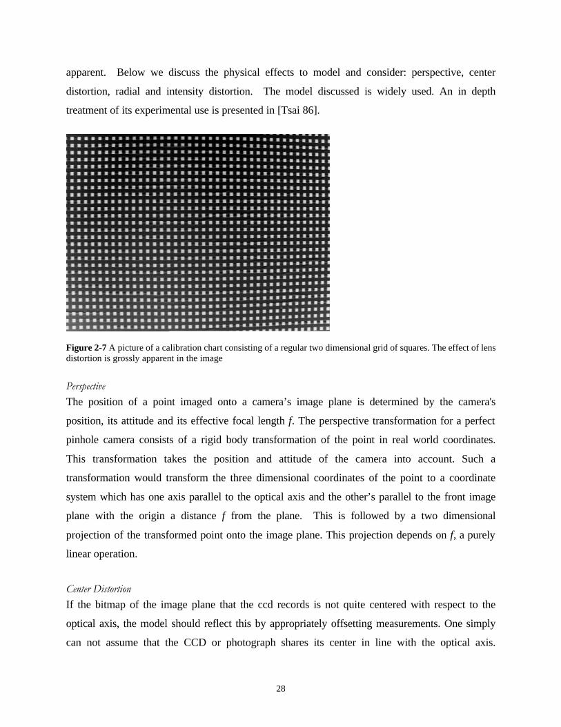
28
apparent. Below we discuss the physical effects to model and consider: perspective, center
distortion, radial and intensity distortion. The model discussed is widely used. An in depth
treatment of its experimental use is presented in [Tsai 86].
Figure 2-7 A picture of a calibration chart consisting of a regular two dimensional grid of squares. The effect of lens distortion is grossly apparent in the image
Perspective
The position of a point imaged onto a camera’s image plane is determined by the camera's
position, its attitude and its effective focal length f. The perspective transformation for a perfect
pinhole camera consists of a rigid body transformation of the point in real world coordinates.
This transformation takes the position and attitude of the camera into account. Such a
transformation would transform the three dimensional coordinates of the point to a coordinate
system which has one axis parallel to the optical axis and the other’s parallel to the front image
plane with the origin a distance f from the plane. This is followed by a two dimensional
projection of the transformed point onto the image plane. This projection depends on f, a purely
linear operation.
Center Distortion
If the bitmap of the image plane that the ccd records is not quite centered with respect to the
optical axis, the model should reflect this by appropriately offsetting measurements. One simply
can not assume that the CCD or photograph shares its center in line with the optical axis.
29
Without an accurate measure of the center, adjusting out radial distortion, which will be
discussed next, is difficult.
Radial Distortion
Pincushion and barrel distortion are the distortions that are apparent as the bowing inward or
outward of images of square objects. This is a radial distortion due to imperfections in the lens.
Short focal length lenses, particularly inexpensive ones, tend to have a fair amount of distortion.
The typical lens, according to [Tsai] can be modeled as having radial distortions that are at most
2nd order. Thus the functional form of the distortion is )||1( 2measuredmeasuredactual PbPP += where
the points referenced have an origin at the point where the optical axis intercepts the image
plane. In experiments [Tsai] has shown the higher order terms contribute insignificantly.
Intensity Distortion
There are two types of intensity distortion in the output signal from a camera. One type is due to
imperfections in the camera lens and is called vignetting. Typically this is instantiated as a sharp
fourth order roll-off in intensity sensitivity around the edges of the lens. The other is a nonlinear
distortion artificially introduced in the output of consumer grade cameras and is called gamma
correction. The output of cheap consumer cameras is designed to be directly input into a
consumer television sets. The cathode ray tubes inside these televisions have a nonlinear
relationship between input voltage and output intensity that is approximately of the form:
γ)(Max
inMaxout V
VII =
Where outI represents the intensity output for a particular pixel, and MaxI represents the maximum
output intensity, inV represents the input voltage to the CRT, and MaxV represents the maximum
input voltage to the CRT. Thus the signal input into these systems must take this effect into
account if one wants an accurate reproduction of the recorded image. This is known as gamma
correction. Note that the gamma of the camera (where gamma of the camera refers to the gamma
that it uses to adjust its output) coupled with quantization due to sampling of the camera input,
determines the fidelity with which the camera can distinguish output intensities; yielding more
fidelity for lower input intensity values for gamma less than one and more fidelity for higher

30
input intensity values for gamma greater than one(note input intensity is related to the inV to the
CRT system described above.)
Having described the camera model, it’s obvious how to calibrate out all the distortions for a
given camera. First one must measure all the parameters of the distortions in the model by taking
pictures of calibration images. The effects of gamma correction need to be factored out first, then
the vignetting. Then, it is possible to remove positional distortions. An important thing to note
about the positional distortions is that they are typically at worst second order and smooth. Now,
having discussed the effects of distortion on the camera image we can move to discussing how to
pick out and measure landmarks in the image.
Automatic Identification of Landmarks and their Measurement
Taking measurements using photographs requires the ability to identify and measure position of
landmarks in a photograph. In this section we will go over some basic machine vision techniques
that can be used to do this. A major assumption is that the landmarks are squares and are easy to
identify and separate from other objects in an image. When calibrating a camera, such scenes are
easy to engineer with a high contrast between the landmark and its background. In such systems
the simple machine vision techniques of thresholding, connecting, and calculating centroids can
be used to identify and measure landmarks to an accuracy higher than the pixel dimensions of the
CCD recording in the image plane. How this works and why it is possible will be explained
below.
Thresholding
In an image where the landmarks stand out in high contrast to the background an easy way to
separate pixels that the landmark covers is by thresholding. The process of thresholding creates a
two-dimensional array exactly the same size as the image bitmap. Each entry is a one if the
corresponding pixel value in the bitmap is greater than or equal to a threshold value or a zero if
the corresponding pixel value in the bitmap is less than the threshold value. The threshold value
has to be picked high enough that the pixels that are greater than the threshold are all part of a
landmark. Connecting the pixels together related to the same landmark is the next step in the
process. With any image it is worth first subtracting out the background, by taking pictures of the

31
background with no landmarks present and subtracting that image from the landmark image.
This makes it so the threshold that needs to be picked to filter out “noise” can be quite low.
Connecting
The image bitmap and threshold array are used to create a connected region array. A connected
region array is the same size as the bitmap and is filled with labels corresponding to the
connected pixels in the bitmap. The assumption is that the threshold that produced the threshold
array was picked low enough so that all the pixels involved with a particular landmark in the
threshold array are adjacent to one another so they may be connected. Pixels are connected if
they neighbor each other on one of four sides and have a corresponding value of one in the
threshold array. Each connected region is given a unique label and this number is placed into the
corresponding element of the connected pixel. The result is a two-dimensional array whose
corresponding pixels in the image bitmap represent landmarks. All pixels related to the same
landmark have the same unique label in the connected region array. Now that the landmarks are
identified and separated, it is possible to measure their centroids.
Measuring Centroids - Super-Resolution
The bitmap and connected region array are then used to create a list of centroids. A two-
dimensional centroid is computed for each connected region. The way to compute the x
coordinate of a centroid for a particular connected region is: average the contributions of the
pixel value multiplied by its x coordinate for each pixel in the bitmap whose element in the
connected region array has the same label as the desired connected region. Say, for example, that
two pixels formed a connected region, then
While the position coordinates on the right hand side of the equation are integers in the bitmap,
the position coordinates on the left need not be an integer. That is the means by which the super-
resolution measurement is achieved beyond that of the camera's CCD's pixel dimensions. Pixel
21
2211 )(
MM
MXMXX centroid +
+=
32
values can range between 0 and 255. Imagine taking a picture of a bright square that extends
over several pixels. The value of a pixel imaging the edge of the square will be determined by
how much of the area of that pixel is covered by that edge. Thus the dynamic range of the
camera can be used to extend the conventional resolution of the camera.
The accuracy of this technique can be estimated by considering the sources of error. One source
of error can be found in the analog electronics that capture the image into the frame buffer(e.g
CCD, and A/D converter). We denote this error errorcamera . errorcamera includes shot noise, and
quantization error. Its value must be calculated based on the specifications of the equipment that
is used to capture the bitmap of the image. The other major source of error comes from the
analytic inaccuracy in the technique of achieving extra precision by taking the centroid of an
image of a square. We denote the other source of error erroranalytic . erroranalytic can be calculated
and below we derive a convenient to use upper bound for it.
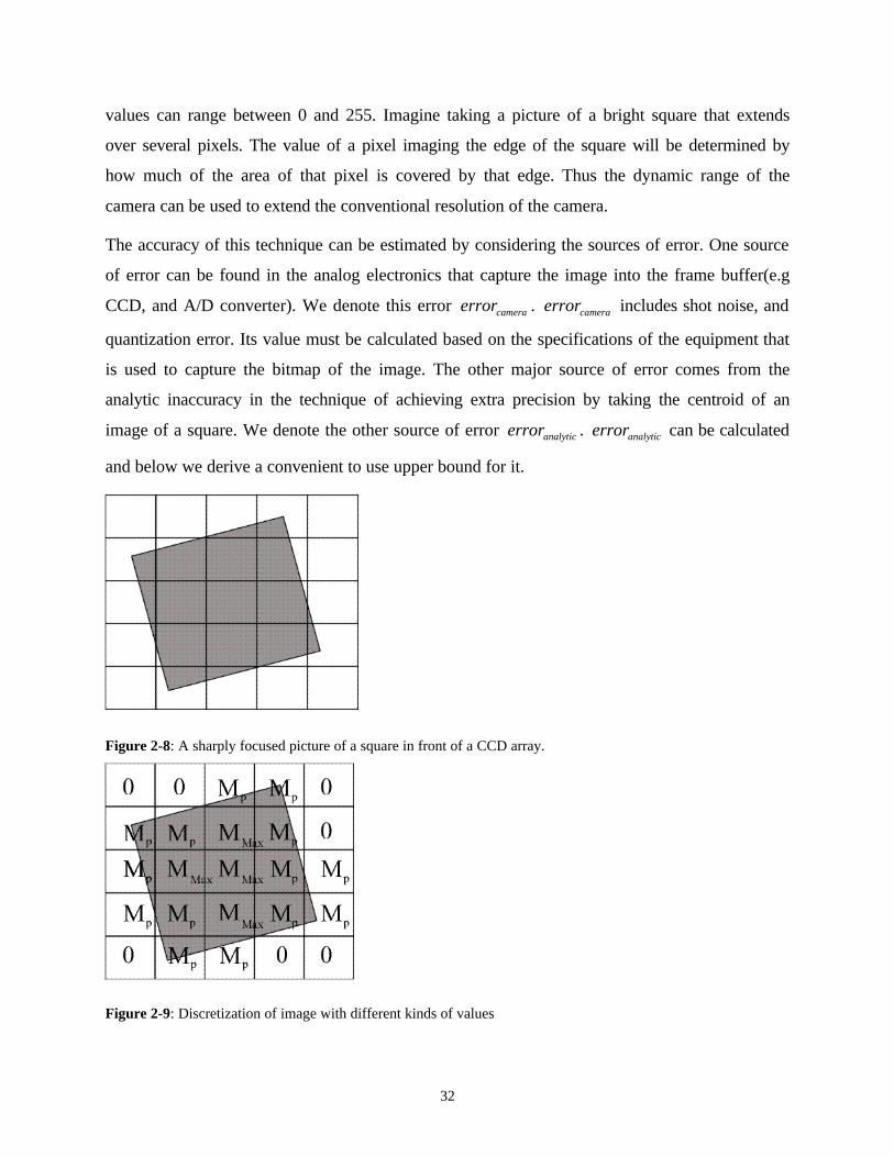
Figure 2-8: A sharply focused picture of a square in front of a CCD array.
Figure 2-9: Discretization of image with different kinds of values
33
Consider the sharply focused continuous image of a square pictured in Figure 2-8 with the
outline of the CCD grid visible. Figure 2-9 represents the discretization of this image into a
bitmap and denotes the three different types of values. The values are based on the amount of
the pixel area covered by the square after the background has been subtracted out. 0 represents
those pixel values that represent pixels that the square does not cover. M p i, represents the value of
the the i th pixel that is partially covered. Mmax represents the value in those pixels that are
totally covered by the square. Note that (1< <M Mp i, max ). N p is the number of partially covered
pixels. N C represents the number of completely covered pixels. One can think of M p i, as the
integration of a constant mass density of value 1
Mmax
over the area of the CCD pixel that is
occluded by the square. The difference between the centroid computed assuming such a mass
density in the real image and the centroid computed using the assumed effective mass is the
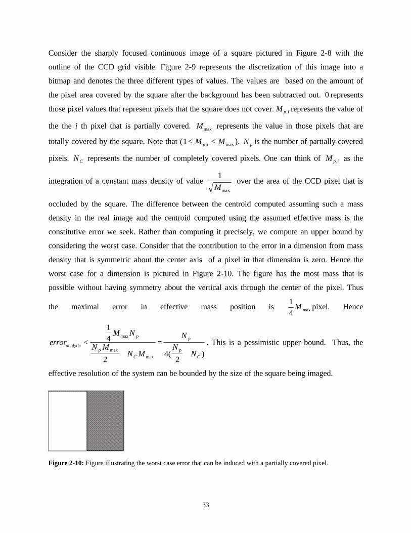
constitutive error we seek. Rather than computing it precisely, we compute an upper bound by
considering the worst case. Consider that the contribution to the error in a dimension from mass
density that is symmetric about the center axis of a pixel in that dimension is zero. Hence the
worst case for a dimension is pictured in Figure 2-10. The figure has the most mass that is
possible without having symmetry about the vertical axis through the center of the pixel. Thus
the maximal error in effective mass position is max4
1M pixel. Hence
errorM N
N MN M
N
NN
analytic
p
p
C
p
p
C
<+
=+
1
4
24
2
max
max
max ( )
. This is a pessimistic upper bound. Thus, the
effective resolution of the system can be bounded by the size of the square being imaged.
Figure 2-10: Figure illustrating the worst case error that can be induced with a partially covered pixel.

34
Finally, the effects of lens distortion on the calculation of the centroid of a small region in a
distorted image can be disregarded because they are second order. One can intuitively see this by
noting that the centroid calculations for small regions about a point are unaffected by the linear
term of the analytic functional expansion about that point.
Which of the aforementioned error terms dominates depends on the input scene and equipment
used to capture the image. However, the estimates provide a means to engineer systems and
images from which the desired accuracy may be extracted.
Figure 2-11: The upper left hand corner of the black square surrounding the number character denotes the centroid of the white square underneath it.
Figure 2-11 shows the successful application of the techniques described here on the picture of
the calibration chart pictured in Figure 2-7. The upper left-hand corner of the black squares with
numbers in them denote the centroid of the white square underneath them.
In this section we have discussed background issues and techniques relevant to digital
photogrammetry as it is used in our prototype system. We plan to use these techniques to
establish the mapping between screen and projector space. Once we have the mappings, using
them to project corrected images will become important. Digital image warping, discussed next
is such a technique.

35
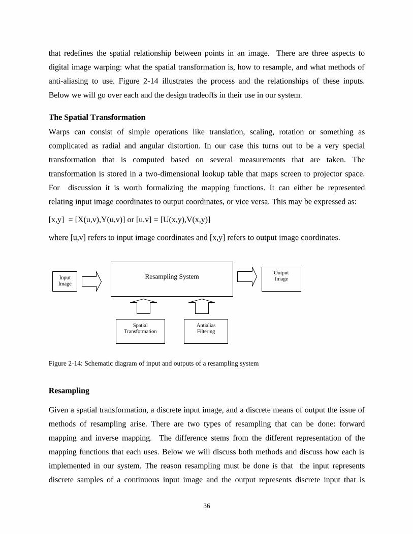
Digital Image Warping Assuming that the functional relationships between screen and projector space have been
measured, one has to warp (map) an image to projector space based on these relationships to
actually display the desired image across the system. The techniques of digital image warping
can be used to do exactly this. In this section we discuss these techniques and the tradeoffs for
using them in our system. For further reading, [Wolberg 90], serves as an excellent reference.
The relevant sections of that book, however, are paraphrased here.
Digital Image Warping is a branch of signal processing which deals with geometric
transformation techniques. It grew out of an interest in the mid-1960s in geometric correction
applications for remote sensing. Figure 6 and 7 illustrate digital image warping done to correct
images sent from NASA's Viking Lander-2 that were distorted. Figure 2-12 is the original
picture distorted due to the downward tilt of the camera on the Lander. Figure 2-13 is the
corrected picture that resulting from digitally warping Figure 2-13. Morphing and texture
mapping are a few of the other special effects that are implemented using digital image warping.
Texture Mapping is so common today in computer graphics that consumer computers often
include hardware to accelerate real-time texture mapping. Warping is essentially an operation
Figure 2-12: Viking Lander picture of moon surface (distorted)
Figure 2-13: Viking Lander picture of moon surface (undistorted)
36
that redefines the spatial relationship between points in an image. There are three aspects to
digital image warping: what the spatial transformation is, how to resample, and what methods of
anti-aliasing to use. Figure 2-14 illustrates the process and the relationships of these inputs.
Below we will go over each and the design tradeoffs in their use in our system.
The Spatial Transformation
Warps can consist of simple operations like translation, scaling, rotation or something as
complicated as radial and angular distortion. In our case this turns out to be a very special
transformation that is computed based on several measurements that are taken. The
transformation is stored in a two-dimensional lookup table that maps screen to projector space.
For discussion it is worth formalizing the mapping functions. It can either be represented
relating input image coordinates to output coordinates, or vice versa. This may be expressed as:
[x,y] = [X(u,v),Y(u,v)] or [u,v] = [U(x,y),V(x,y)]
where [u,v] refers to input image coordinates and [x,y] refers to output image coordinates.
Resampling
Given a spatial transformation, a discrete input image, and a discrete means of output the issue of
methods of resampling arise. There are two types of resampling that can be done: forward
mapping and inverse mapping. The difference stems from the different representation of the
mapping functions that each uses. Below we will discuss both methods and discuss how each is
implemented in our system. The reason resampling must be done is that the input represents
discrete samples of a continuous input image and the output represents discrete input that is
Figure 2-14: Schematic diagram of input and outputs of a resampling system
Input Image
Resampling System
Spatial Transformation
Antialias Filtering
Output Image

37
made into a continuous signal by the projection system. We don’t have the continuous input
image. Resampling is the means of interpolating the continous input image from that discretized
input image and then sampling at a point in the continuous input image space related to the
output projector space by the spatial transformation.
Forward Mapping.
Figure 2-15: One-dimensional forward mapping
Forward Mapping uses the [X(u,v),Y((u,v)] representation of the transformation to map input to
output. Each input pixel is passed through the process where it is mapped to a new output
coordinate. Note that each input pixel coordinate is mapped from integer coordinates to the real
numbers. In Figure 2-15 this is illustrated by regularly spaced input and irregularly spaced
output. Notice that some of the output points are missed. The real valued output presents
complications, possibly leaving holes of discrete output values unmapped. One can avoid this by
filling in values missed based on the neighboring values. A good way to do this maps the four-
corners of a pixel rather than just the center. This maps square patches to quadrilaterals in the
output, rather than single points. Figure 10 illustrates this idea. Assuming the four corner
mapping, an additional consideration is that the mapping could take whole sets of four corners
and map them within a single output pixel or across several in which case a better means of
output is to use an accumulator array at the output and integrate the respective contributions to an
output pixel based on the percentage of the output pixel covered by the output quadrilateral. This
requires expensive interpolation tests and thus is unfortunately very expensive. Traditionally this
problem is dealt with by adaptively sampling of the input such that the projected area from a
single pixel is approximately one pixel in the output space. At that point the contributions from
each input pixel and numbers of input pixels contributing to an output pixel start converging to
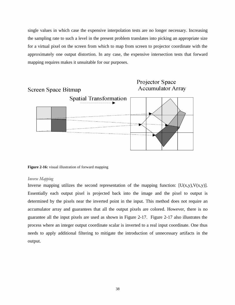
38
single values in which case the expensive interpolation tests are no longer necessary. Increasing
the sampling rate to such a level in the present problem translates into picking an appropriate size
for a virtual pixel on the screen from which to map from screen to projector coordinate with the
approximately one output distortion. In any case, the expensive intersection tests that forward
mapping requires makes it unsuitable for our purposes.
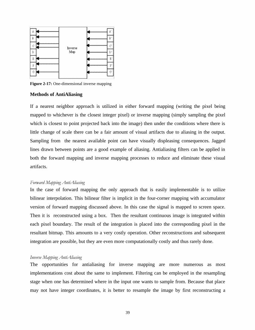
Inverse Mapping
Inverse mapping utilizes the second representation of the mapping function: [U(x,y),V(x,y)].
Essentially each output pixel is projected back into the image and the pixel to output is
determined by the pixels near the inverted point in the input. This method does not require an
accumulator array and guarantees that all the output pixels are colored. However, there is no
guarantee all the input pixels are used as shown in Figure 2-17. Figure 2-17 also illustrates the
process where an integer output coordinate scalar is inverted to a real input coordinate. One thus
needs to apply additional filtering to mitigate the introduction of unnecessary artifacts in the
output.
Figure 2-16: visual illustration of forward mapping
39
Methods of AntiAliasing
If a nearest neighbor approach is utilized in either forward mapping (writing the pixel being
mapped to whichever is the closest integer pixel) or inverse mapping (simply sampling the pixel
which is closest to point projected back into the image) then under the conditions where there is
little change of scale there can be a fair amount of visual artifacts due to aliasing in the output.
Sampling from the nearest available point can have visually displeasing consequences. Jagged
lines drawn between points are a good example of aliasing. Antialiasing filters can be applied in
both the forward mapping and inverse mapping processes to reduce and eliminate these visual
artifacts.
Forward Mapping AntiAliasing
In the case of forward mapping the only approach that is easily implementable is to utilize
bilinear interpolation. This bilinear filter is implicit in the four-corner mapping with accumulator
version of forward mapping discussed above. In this case the signal is mapped to screen space.
Then it is reconstructed using a box. Then the resultant continuous image is integrated within
each pixel boundary. The result of the integration is placed into the corresponding pixel in the
resultant bitmap. This amounts to a very costly operation. Other reconstructions and subsequent
integration are possible, but they are even more computationally costly and thus rarely done.
Inverse Mapping AntiAliasing
The opportunities for antialiasing for inverse mapping are more numerous as most
implementations cost about the same to implement. Filtering can be employed in the resampling
stage when one has determined where in the input one wants to sample from. Because that place
may not have integer coordinates, it is better to resample the image by first reconstructing a
Figure 2-17: One-dimensional inverse mapping

40
continuous representation around that point based on the samples available and resampling that
representation at the point that you want. In the ideal case a sync function would be used to
perfectly reconstruct the input, but alas such a function has infinite support and is thus not
computable given our input. Fortunately there are many substitutes for interpolation kernels like
the Windowed Sync, Lanczos window, Hamming Window, cubic spline, cubic convolution,
exponential and linear. [Wolberg] gives an excellent description of all these methods along with
a comparison. It becomes obvious from his experiments in his book that the difference between
nearest neighbor and linear interpolation is extreme and visually worth correcting,but beyond
that the benefit to effort ratio can be miniscule. Of course this also depends on the image being
resampled and the grid to which it is being warped.
Conclusion In this chapter we have provided background and techniques relevant to creating an
automatically calibrated edge-blended projection array. In the following chapters we will use the
techniques and report experimental results. The next chapter begins with the set of results from
deriving the mapping from projector to screen space.

41
Chapter 3 Establishing the Positional Mappings The two roles that the positional mappings serve are to provide the relative sub-pixel registration
among the projector channels in the overlap regions and to provide the absolute geometric
correction of the projected image across the system. This chapter is divided into two sections.
Each section discusses the design and effectiveness of the methods used to extract the
information necessary to derive a positional mapping from projector to screen space that can
perform these roles.
Sub-pixel Registration In order to achieve sub-pixel registration in the overlap regions among the projector channels,
let’s consider the effective camera resolution that must be achieved. We can choose to restrict the
part of the image that is used to the inner 400 by 400 pixels of our 510 by 490 pixel CCD camera
to attenuate the effects of vignetting. Assuming a twenty percent overlap in each linear
dimension of the 800 by 600 pixel projectors, the approximate resolution of our 2 by 2 projector
system will be 1320 by 960. Thus a conservative estimate is that 2.7 bits beyond the resolution of
the CCD are necessary to guarantee at least a ¼ pixel overlap in each dimension.
The estimated errors can be used to design images to project that should allow us to
achieve the necessary resolution for the camera space to projector space mapping. Let’s first
consider erroranalytic derived in the prior chapter. If we project squares that are greater than eight
pixels by eight pixels on the camera CCD then erroranalytic < = <28
4 641093
1
22 7*( )
. . . From the
specifications of the camera and frame grabber errorcamera = 56 db in intensity. That means that
the camera intensity range is truly eight bits. Clearly an error of less than256
1 in intensity will
have miniscule impact when compared with the error induced by the analytic approximation. In
consideration of the total error, as long as we image landmarks of the prescribed size we should
be able to achieve resolution that is of the desired accuracy.
Rather than projecting individual squares and measuring the centroid for each pixel, we measure
the centroids for an evenly spaced two dimensional grid in each projector space. The resultant
table can be used to interpolate the location in camera space of all other pixels in that projector’s

42
space. The measurement of these points is done in parallel, by projecting images whose spacing
eliminates screen flare effects. Figure 3-1 illustrates an example of such an image.
Figure 3-1: Image of test chart projected to determine camera to screen space mappings.
The result of an experiment that projected a random sample of interpolated registered points
across the system resulted in an indirect measurement of the accuracy achieved was positive but
mixed. In the vertical direction the measured pixel registration for 20 points was within the ¼
pixel desired. In the horizontal direction, however, we achieved less than that with a few pixels
actually not overlapping. Upon examination of the images the registration accuracy in those area
revealed that the images did not have the desired square size specified. The actual number of
pixels covered by a relevant landmark was more consistent with five by five squares, or an error
of 4/1)98(4
16<
+ which provides at worst a resolution the size of one projected pixel in the
horizontal direction hence the resultant non-overlap. Undoubtedly more careful implementation
using larger landmarks would address this issue and achieve the desired sub-pixel registration.
Nonetheless a large fraction of the pixels do achieve the desired accuracy, so the resultant system
is usable.
Total Geometric Correction Having effectively registered the pixels in deriving the projector space to camera space mapping,
we can address the issue of total geometric correction. Total geometric correction can be

43
achieved by measuring and factoring out the positional distortions due to the lens and the
position and attitude of the camera. In our system measuring a screen space to camera space
mapping accomplishes this. A geometrically correct calibration chart is imaged and turned into a
two-dimensional table representing the mapping from screen to camera space. The resultant
mapping can than be composed with the prior projector to camera space mappings to create the
mapping from each projector space to screen space. In this section we will first discuss the
design of our screen space to camera space measurement. Then we will measure the
effectiveness of the approach by measuring the geometric distortion in a composed mapping.
While it is easy to estimate an accuracy that can be achieved measuring centroids of landmarks
in camera space, it is difficult to estimate the accuracy achieved in measuring the parameters of
lens distortion for an as yet unmeasured. Our approach is to take a picture of a regular two-
dimensional grid in screen space, as pictured in Figure 6 in chapter 2. The centroids of the
squares are computed and then used as input to a least squares fit to a cubic consistent with the
assumed second order distortions. Here we are using our knowledge of the physics to increase
the accuracy of our measurement and provide the smoothness that linear interpolation between
measured points won’t. The chart was generated using a plotter and the squares are 10 mm wide
and 20 mm apart. The size of the chart was chosen both to limit the total square distortion, yet
achieve sub camera pixel accuracy and provide lots of samples for the least squares fits.
We can directly measure the accuracy of the approach to correcting the total geometric distortion
by composing the mapping from each projector space to camera space with that of the screen
space to camera space mapping. We will first discuss how to compose the mapping. Then we
will provide results from projecting a two-dimensional graph-paper like grid across the system.
The screen space to camera space mapping and the projector space to camera space mapping are
both one to one. As long as the screen space projected into camera space covers all the projector
space than one can derive a mapping using the two-dimensional tables and approximate
functional inversion using a bilinear approximation for points within known data points. Camera
space serves as an intermediary space that can be composed out. The result is the screen space to
projector space mapping represented as a two-dimensional lookup table. One can invert the
mapping using a simple bilinear approximation with the inversion of neighboring points as it
suits the application.
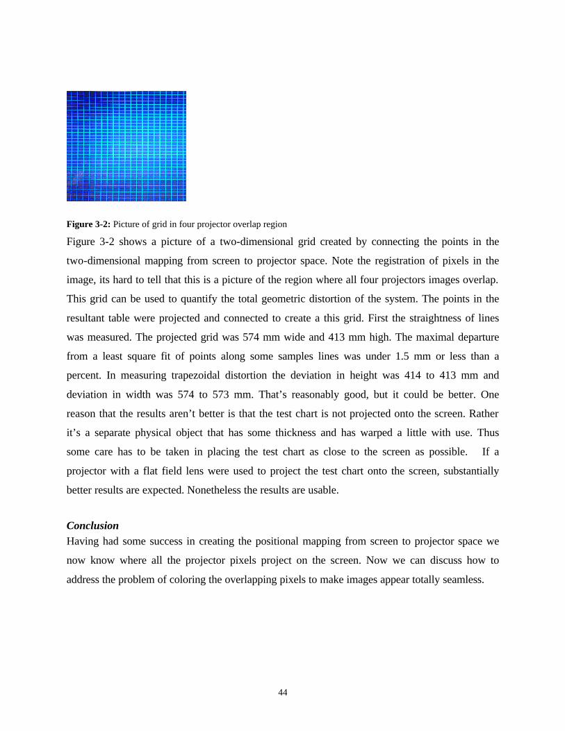
44
Figure 3-2: Picture of grid in four projector overlap region
Figure 3-2 shows a picture of a two-dimensional grid created by connecting the points in the
two-dimensional mapping from screen to projector space. Note the registration of pixels in the
image, its hard to tell that this is a picture of the region where all four projectors images overlap.
This grid can be used to quantify the total geometric distortion of the system. The points in the
resultant table were projected and connected to create a this grid. First the straightness of lines
was measured. The projected grid was 574 mm wide and 413 mm high. The maximal departure
from a least square fit of points along some samples lines was under 1.5 mm or less than a
percent. In measuring trapezoidal distortion the deviation in height was 414 to 413 mm and
deviation in width was 574 to 573 mm. That’s reasonably good, but it could be better. One
reason that the results aren’t better is that the test chart is not projected onto the screen. Rather
it’s a separate physical object that has some thickness and has warped a little with use. Thus
some care has to be taken in placing the test chart as close to the screen as possible. If a
projector with a flat field lens were used to project the test chart onto the screen, substantially
better results are expected. Nonetheless the results are usable.
Conclusion Having had some success in creating the positional mapping from screen to projector space we
now know where all the projector pixels project on the screen. Now we can discuss how to
address the problem of coloring the overlapping pixels to make images appear totally seamless.

45
Chapter 4 Establishing a Color and Intensity Mapping The solution to coloring projector pixels so that there are no perceivable seams is to create a
color and intensity mapping for each output pixel that takes into account the intensity and
overlap distortions between and among the projectors. This mapping can be used to warp or pre-
distort input images appropriately. The mapping can be created through the measurement of the
distortions, using both the positional relationships all ready established along with the projectors
and camera. In this chapter we will specify what it takes to be seamless, how we can achieve
this, and then discuss and evaluate some results from an implementation.
What does it take to be seamless? The background chapter suggests that in order for a system to be imperceivably seamless when
displaying uniformly colored images the intensity may vary at most 2 percent across a degree of
view. In order for color mixing to work, these intensity variations when viewed through filters
representing the eyes spectral responses of long, medium and short cones must also vary in the
same manner or we will perceive a smooth variation of colors. As long as the mapping created
can reproduce uniformly colored images with these properties the system will display seamless
images.
How can we establish the mapping with our system? Establishing a mapping across the spectrum of intensity and color presupposes an ability to
display a single uniform color across the system. First we will discuss how our system can
display a uniformly colored image. Then we will discuss how our system can measure this. Then
we will discuss how to establish the mapping necessary to display a uniformly colored image.
After that the technique of using the solution to the uniform color and intensity problem to create
the table(mapping) that spans all intensities and colors will be described.
How to Display a Uniformly Colored Image
The means and implementation are exactly the same as discussed in the background section on
edge-blended projector arrays. We have exactly the same physical setup but the physical means
is worth some review since it provides some insight into the makeup and limitations of our
mapping. In a single projector systems, three separate channels: red, green, and blue are
converged at a point to allow a pixel to span the perceivable spectrum. Since our projection

46
systems all use the same filters and light sources, any particular point is still illuminated by three
channels of red, green and blue spectrums. Though in the regions where n projectors overlap we
can control the contribution to each channel from each projector. By carefully choosing the
contributions from each projector to the red, green and blue channels for each intensity and color
to be displayed across the system we should be able to project a uniformly colored image. One
means of doing this smoothly in the overlap regions is to relatively weight a projector’s
contribution to a point based on how far it is to its closest projected edge as compared with the
other projectors contributing to the same point. The limitations of the system are that each
projector’s channel has a minimum light intensity. The sum of these determines the black level
for each pixel. This means there is a minimum intensity that we can display for each channel at
each point. Similarly there is a maximum. In any case we will now discuss how we can measure
and determine these contributions with our feedback camera.
How to Measure a Uniform Image
One of our assumptions is that the camera views an image similar to the one from other
viewpoints. In other words we need a wide exit pupil. Thus we must use a screen with a gain
near one. The limits of this exit pupil will depend on both the actual gain and the error in the
camera. But the point is if we don’t do this than the uniformly colored image viewed from the
camera viewpoint won’t be uniformly colored from another viewpoint. This would limit the
utility of the system.
We have an eight-bit monochrome feedback camera viewing the projected image. We can
certainly eliminate intensity distortions like gamma correction, vignetting and distance effects by
measuring their effect and factoring it out. Thus its is possible to measure a uniform intensity,
though the vignetting and gamma correction may further limit the dynamic range of 8 bits. Since
the projectors use red, green, and blue channels to reproduce color we can use red, green, and
blue filters on a monochrome camera to factor out the black levels of the other colors in our
measurements. Thus it is also possible to measure uniform red, green and blue across the system.
If the image using each filter is uniform than there sum which is what is viewed will be uniform.
Thus it is then possible to view a uniformly colored image of any color.
The actual error in intensity and color variation depends on whether or not we have factored out
the lens distortions. In our current set up the lens intensity distortions are limited by having the

47
camera axis close to perpendicular to the screen, limiting the usable are of the CCD to the inner
part to lower the effect of vignetting, and using a camera with a gamma of one. We will
indirectly measure the results of this decision in our results section.
Establishing a Uniformly Colored Image.
So now that we know that the system can produce and measure a uniformly bright color, how
can we use the system to find out what the image input to the projector has to be to do this for a
particular color and brightness. The one approach that immediately comes to mind in trying to
solve this problem is to follow the strategy used before in establishing a positional mapping:
taking one set of measurements and computing the desired mapping. Also taking into account all
the issues mentioned in the background section. That approach is complicated by the amount of
modeling that needs to be done. A more practical solution is to use the system itself in a
feedback loop iterating to find a fixed point that is the desired answer. Both approaches are
worth discussing, the first because doing so will shed some light on the physical nature of the
problem, and the second because it’s the one that is practical.
The Measure, Model and Compute Approach
In the first approach a set of test patterns like the ones used for creating the positional warp
mappings with grids of isolated squares are projected. Intensities of these squares are varied; thus
sampling the space and thus creating a table of measurements from which interior points may be
Figure 4-1: Model of effects of illumination
ii yx βα ),(
)( jj vg
∑
jβ
),,( byxfjq
),( yxb
48
linearly interpolated. From such measurements it is possible to construct the desired table based
on a model of addition in the overlap region as well as the illumination affect of adjacent pixels.
(Rather, this “effect” is really just the effect of the point spread function when the output is
thought of as the projection of the two-dimensional analog of an impulse train, convolved with a
point spread function that represents the effects of the screen and pixel width)
Figure 4-1 gives a model of the measured output iq from the camera for each projector pixel i.
The value measured is a function of the camera’s position and orientation, the particular pixels
input value iv , and value of all the other pixels around it. More specifically for each pixel j there
is a transfer function jg that maps input values to output intensity contributions jβ .
Correspondingly there is a camera transfer function for each screen position that maps brightness
b(x,y) to camera measurement jq . Figure 4-1 illustrates these relationships and the coupling. The
summing of light is accounted for by the adder. It adds up illumination contributions from other
pixels. The scalars ),( yxiα are used to denote whatever effect geometry has on the
illuminations from pixel i. The point in showing these functional relationships is to show the
nature of the coupling between input intensities and output intensities - how changing a pixel's
color has an effect across the system. While the coupling is not strong, it is empirically
measureable. In order to construct a solution to displaying a single intensity across the system
one needs to know g, and the alphas. Thus one must construct a methodology to compute and
measure these. The end result here is a model that allows one to compute the intensity measured
at any one point based on all the input pixel values for all the projectors. Thus to display a
uniform color across the system, one needs to solve the equations that form the model adding
the constraints of the overlapping regions etc. Still that's thousands of coupled equations that
need to be solved. Iteration would be a practical way to solve this numerical problem. With the
solution in hand, one would then display the result and measure the error. That would provide
some measure of what was "wrong" with the model. The problem that is being solved is not
"what is wrong with the model" however. The problem is to get the projectors to project a
uniform intensity for a particular color. A smaller error would be appreciated more, and since the
system is set up there is a more practical and better approach that will be discussed next.
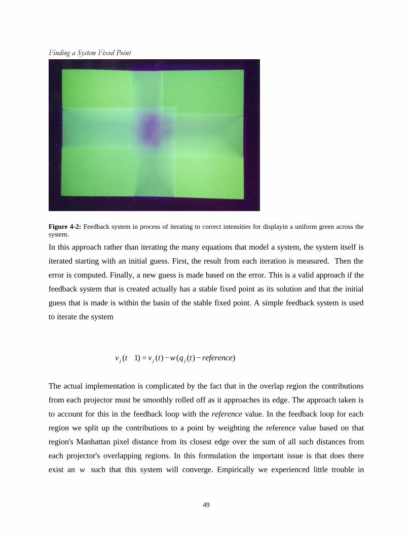
49
Finding a System Fixed Point
Figure 4-2: Feedback system in process of iterating to correct intensities for displayin a uniform green across the system.
In this approach rather than iterating the many equations that model a system, the system itself is
iterated starting with an initial guess. First, the result from each iteration is measured. Then the
error is computed. Finally, a new guess is made based on the error. This is a valid approach if the
feedback system that is created actually has a stable fixed point as its solution and that the initial
guess that is made is within the basin of the stable fixed point. A simple feedback system is used
to iterate the system
The actual implementation is complicated by the fact that in the overlap region the contributions
from each projector must be smoothly rolled off as it approaches its edge. The approach taken is
to account for this in the feedback loop with the reference value. In the feedback loop for each
region we split up the contributions to a point by weighting the reference value based on that
region's Manhattan pixel distance from its closest edge over the sum of all such distances from
each projector's overlapping regions. In this formulation the important issue is that does there
exist an ω such that this system will converge. Empirically we experienced little trouble in
))(()()1( referencetqtvtv jjj −−=+ ω

50
finding such a value. The speed of convergence is also an important issue, typically we observed
the system converging in under 20 iterations. Additionally, as far as good initial guesses, we can
only offer empirical evidence that the system converges by starting with zero as input. Typically
values of .3 seem to work fine in terms of fast convergence. Figure 4-2 shows a feedback loop in
the middle of calibrating a single color intensity(green). Notice that the regions of overlap are
still being corrected. Figure 4-3 shows the output from a single projector displaying a portion of
an image. Please note the roll off at the edges and the edge effects of the Manhattan metric.
It’s worth noting, finally, that rather than storing this mapping for each pixel we store the values
for a subset of the pixels. Then the value for any particular pixel can be interpolated from the
stored values of pixels surrounding it.
Figure 4-3: Picture of a single projector displaying its portion of an image
Creating the Mapping With a solution for creating a uniformly bright intensity the strategy for creating the mapping can
be discussed. For a particular color: red, green, or blue it is possible to display a uniformly bright
intensity. By sampling the inputs necessary to create a set of appropriately chosen output
intensities the desired mapping for a particular color and position can be established in the form
of a lookup table. The output value for input points between sampled points can be linearly
interpolated from the map for that position. In practice, six points uniformly strewn across the
output intensity spectrum provides adequate results. Depending on the projection system this
process can be repeated for each color: red, green or blue. For example, in a system where a
51
color wheel is employed one need only calibrate one color. In a system where three imaging
units are used, sampling all three might be necessary. In our Epson system that has three separate
channels, slightly better results were derived from measuring lookup tables for all three colors
rather than just one color.
Implementation Results: Figure 4-4 illustrates the systems ability to mix colors with a picture of the system trying to
display a high intensity white. The results are visually satisfactory, though residual effects of the
manhattan metric can be observed in the output near the seams. Upon closer observation using a
light meter to measure the uniformity of brightness the reason for this becomes more apparent.
The actual output of the system is about 40 percent brighter at the edges than in the center of the
full screen when a bright white image is displayed. The camera measurement is, however, quite
uniform, but its internal intensity distortions due to vignetting were not calibrated out in the
implementation. Thus the system could use some further correction. This error indirectly
suggests that the intensity distortion vary as much as 40 percent from the center to the edge of
the lens. However as far as this system is concerned the uniformity in brightness in white
perceived is acceptable for viewing angles where the image arc from the center to the edge is
greater than 20 degrees. It could be better. Figure 4-5 illustrates the black level of the system
illustrating the non-uniformity tradeoff discussed earlier for getting high contrast ratio in the
areas where there is no overlap. The contrast ratio for the system thus varies from 28.5 in the
region of quadruple overlap to 145 with no overlap.

52
Figure 4-4: Picture of system displaying all white.
Figure 4-5: Picture of system displaying all black
Conclusion In this chapter the issues, methodology, implementation of creating and using intensity and color
mappings to make completely seamless images were discussed. The implementation clearly
showed it was possible to create a totally seamless display of uniformly colored pictures. The

53
drawbacks of the current implementation were also discussed. Now we will discuss coupling this
mapping with the positional mapping to display uniformly bright images.

54
Chapter 5 Using the Mappings: A Seamless Display In order to display pleasing moving pictures across our seamless video wall, our digital image
warper that utilizes the mappings derived from prior chapters must be designed to work in real-
time and make effective use of the resolution provided. Below we discuss how the real-time
issue affects our choice of warping style and resampling algorithms. The chapter finishes by
evaluating how effectively we have utilized the available resolution in projecting a seamless
image.
Warping Style While the relationship between screen space and projector space has all ready been determined,
we haven’t prescribed the direction of the functional transformation. The choice of warping
style, inverse mapping or forward mapping, determines that direction and can have dramatic
impact on performance. Forward mapping utilizes expensive intersection tests. Primarily for this
reason, it is not generally implemented in real-time warping engines. As was discussed in greater
detail in the background chapter, inverse warping is better suited for real-time applications than
forward warping. Thus we have chosen to use inverse mapping as our warping style. This means
that the direction of the functional transformation is from projector space to screen space. Note
that we associate an input bitmap image with screen space by positioning it to be displayed
within the largest displayable rectangle in screen space. Thus once we have the screen space
coordinate associated with a projector pixel we can resample the input bitmap based on the latter
mentioned relationship between the input bitmap and screen space. Having discussed the effect
of the real-time constraint on our choice of warping style we can discuss how it effects
resampling.
Resampling The real-time constraint conflicts with our ability to perfectly reconstruct images; convolution
with a sync function with infinite support is not possible in a finite time. There are however a
wide variety of approximations that can be used: nearest neighbor, bilinear interpolation, etc…
All of these methonds can be easily implemented in hardware when inverse warping is used.
There is a great body of literature from the late seventies and early eighties comparing and
contrasting the results of using these methods [Wolberg 90]. Figure 5-1 through Figure 5-5
55
provide a visual comparison of the different methods in the context of our system. Figure 5-1
through Figure 5-3 are images of the system displaying a sinusoid in intensity. Figure 5-1 shows
the visible drawback of using the nearest neighbor technique. The blocky appearance and jagged
edges visible when displaying regions of high frequency in images are consistent with one would
expect. Figure 5-2 showing linear interpolation is remarkably better. Figure 5-3 showing perfect
reconstruction is provided for contrast; its better and thus demonstrates the tradeoff. Figure 5-4
and Figure 5-5 further contrast the two techniques on an everyday image of a typical computer
screen bitmap. The “jaggies” (the jagged lines outlining a window) and the jagged text visible in
Figure 5-4 give away the nearest neighbor sampling used to create it, while the effectiveness of
the bilinear filtering in making a sharp window line and text is apparent in Figure 5-5.
For now we have chosen to use bilinear interpolation as our resampling strategy. Thus the real-
time constraint visibly impacts the output quality by requiring less than optimal filtering of input
images. Linear interpolation provides output of acceptable quality. The output quality could be
improved by implementing better filtering. Having discussed the resampling algorithm we can
now discuss the effective resolution of the system.
Effective Resolution: What Resolution is the System? Ascribing a resolution to the system is not straightforward. A first order measure that serves as
an upper bound for an M by N array of projectors with resolutions of Q by R pixels is MNQR.
However due to the overlap and geometric distortion the vertical and horizontal resolution of the
largest rectangle that can be inscribed within the bounds of the projected area is somewhat less
than that. The number of pixels one can count while tracing a line from left to right or top to
bottom can vary quite extensively. For example, in the 2 by 2 array of 800 by 600 pixel
projectors in the prototype system (1600 by 1200 theoretical), a sampling of lines drawn from
top to bottom varies from 1230 pixels to 1300 pixels, and from left to right from 900 pixels to
1000 pixels. By no means does that represent a regular grid of pixels. We can however use these
samples to conservatively ascribe a resolution consistent with the lowest numbers: 1290 by 900.
We can measure the effectiveness of how our system uses the provided resolution by measuring
the modulation transfer function of our system assuming the measured resolution. The transfer
functions were measured by inputting bitmap images of sinusoids of varying frequency and
measuring the contrast ratio between the highest value and lowest value measured along periods
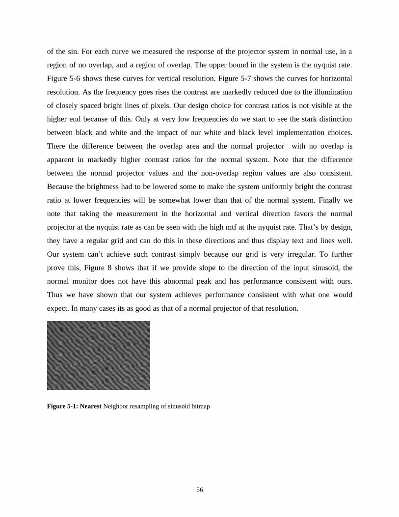
56
of the sin. For each curve we measured the response of the projector system in normal use, in a
region of no overlap, and a region of overlap. The upper bound in the system is the nyquist rate.
Figure 5-6 shows these curves for vertical resolution. Figure 5-7 shows the curves for horizontal
resolution. As the frequency goes rises the contrast are markedly reduced due to the illumination
of closely spaced bright lines of pixels. Our design choice for contrast ratios is not visible at the
higher end because of this. Only at very low frequencies do we start to see the stark distinction
between black and white and the impact of our white and black level implementation choices.
There the difference between the overlap area and the normal projector with no overlap is
apparent in markedly higher contrast ratios for the normal system. Note that the difference
between the normal projector values and the non-overlap region values are also consistent.
Because the brightness had to be lowered some to make the system uniformly bright the contrast
ratio at lower frequencies will be somewhat lower than that of the normal system. Finally we
note that taking the measurement in the horizontal and vertical direction favors the normal
projector at the nyquist rate as can be seen with the high mtf at the nyquist rate. That’s by design,
they have a regular grid and can do this in these directions and thus display text and lines well.
Our system can’t achieve such contrast simply because our grid is very irregular. To further
prove this, Figure 8 shows that if we provide slope to the direction of the input sinusoid, the
normal monitor does not have this abnormal peak and has performance consistent with ours.
Thus we have shown that our system achieves performance consistent with what one would
expect. In many cases its as good as that of a normal projector of that resolution.
Figure 5-1: Nearest Neighbor resampling of sinusoid bitmap

57
Figure 5-2: Bilinear Interpolation resampling of sinusoid bitmap
Figure 5-3: Perfect resampling of sinusoid bitmap
Figure 5-4: Normal bitmap Displayed on System using nearest neighbor resampling.

58
Figure 5-5: Normal bitmap displayed on system using linear interpolation resampling
MTF Vertical (Contrast vs Frequency)
0
5
10
15
20
0 0.2 0.4 0.6 0.8 1 1.2
fraction of nyquist
No Overlap
Overlap
Normal Monitor
Figure 5-6: Vertical MTF
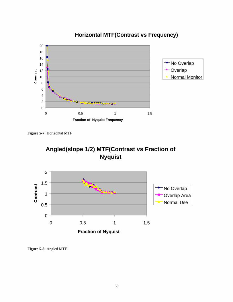
59
Horizontal MTF(Contrast vs Frequency)
0
2
4
6
8
10
12
14
16
18
20
0 0.5 1 1.5
Fraction of Nyquist Frequency
No Overlap
Overlap
Normal Monitor
Figure 5-7: Horizontal MTF
Angled(slope 1/2) MTF(Contrast vs Fraction of Nyquist
0
0.5
1
1.5
2
0 0.5 1 1.5
Fraction of Nyquist
No Overlap
Overlap Area
Normal Use
Figure 5-8: Angled MTF

60
Conclusion By using a digital image warper that inverse maps and uses bilinear interpolation we have
implemented a system that can work in real-time and can display seamless images consistent
with the resolution provided and with some trade off for contrast.

61
Chapter 6 Conclusions and Future Work This thesis has presented techniques for combining high performance computing with feedback
to enable the correction of imperfections in the alignment, optical system and fabrication of very
high-resolution display devices. The key idea relied on the measurement of relative alignment,
rotation, optical distortion, and intensity gradients of an aggregated set of image display devices
using a precision low cost reference. Use of the reference made it possible to construct a locally
correct map relating the coordinate system of the aggregate display to the coordinate system of
the individual projectors. The techniques form a new technology for scalable, bright, seamless,
high-resolution large-scale self-calibrating displays (seamless video walls). The technology
aggregates low-cost component displays and allows one to linearly scale up resolution or size
while maintaining a single level of brightness. None of the well-known technologies for creating
large-scale displays are portable, scalable and provide results that are as visually satisfactory.
The manual calibration and necessary precision involved in those technologies is too great to be
scalable; the automatic calibration approach espoused in this thesis is far superior and enables
scalability. Low cost computation coupled with feedback is leveraged to provide the necessary
precision, and thus correct all distortions digitally. The successful construction of a prototype
seamless video wall that requires no manual alignment provides ample evidence of the validity
of the techniques in this thesis. Below the conclusions from constructing the prototype system
and suggestions for further work given.
Conclusions The prototype system consisting of a two by two array of projectors was arranged to project
overlapping images with a camera used for feedback. Photogrammetry, machine vision and
digital image warping techniques were composed to couple computation, feedback and
projectors to make a single seamless image appear across the aggregated projection displays. The
photogrammetry and machine vision were used with the feedback to create the locally correct
maps relating the coordinate system of the aggregate display to the coordinate systems of the
individual projectors. Camera distortions are computed from a picture taken of a low-cost
precision reference. Then calibration images are projected, captured and undistorted yielding the
desired mapping from the screen to each projector. The resultant mappings provide a means for
positionally warping an input image to appear positionally seamless. From these mappings one
can digitally warp the desired displayed image to appear positionally seamless across the
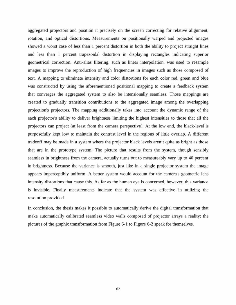
62
aggregated projectors and position it precisely on the screen correcting for relative alignment,
rotation, and optical distortions. Measurements on positionally warped and projected images
showed a worst case of less than 1 percent distortion in both the ability to project straight lines
and less than 1 percent trapezoidal distortion in displaying rectangles indicating superior
geometrical correction. Anti-alias filtering, such as linear interpolation, was used to resample
images to improve the reproduction of high frequencies in images such as those composed of
text. A mapping to eliminate intensity and color distortions for each color red, green and blue
was constructed by using the aforementioned positional mapping to create a feedback system
that converges the aggregated system to also be intensionally seamless. Those mappings are
created to gradually transition contributions to the aggregated image among the overlapping
projection's projectors. The mapping additionally takes into account the dynamic range of the
each projector's ability to deliver brightness limiting the highest intensities to those that all the
projectors can project (at least from the camera perspective). At the low end, the black-level is
purposefully kept low to maintain the contrast level in the regions of little overlap. A different
tradeoff may be made in a system where the projector black levels aren’t quite as bright as those
that are in the prototype system. The picture that results from the system, though sensibly
seamless in brightness from the camera, actually turns out to measureably vary up to 40 percent
in brightness. Because the variance is smooth, just like in a single projector system the image
appears imperceptibly uniform. A better system would account for the camera's geometric lens
intensity distortions that cause this. As far as the human eye is concerned, however, this variance
is invisible. Finally measurements indicate that the system was effective in utilizing the
resolution provided.
In conclusion, the thesis makes it possible to automatically derive the digital transformation that
make automatically calibrated seamless video walls composed of projector arrays a reality: the
pictures of the graphic transformation from Figure 6-1 to Figure 6-2 speak for themselves.
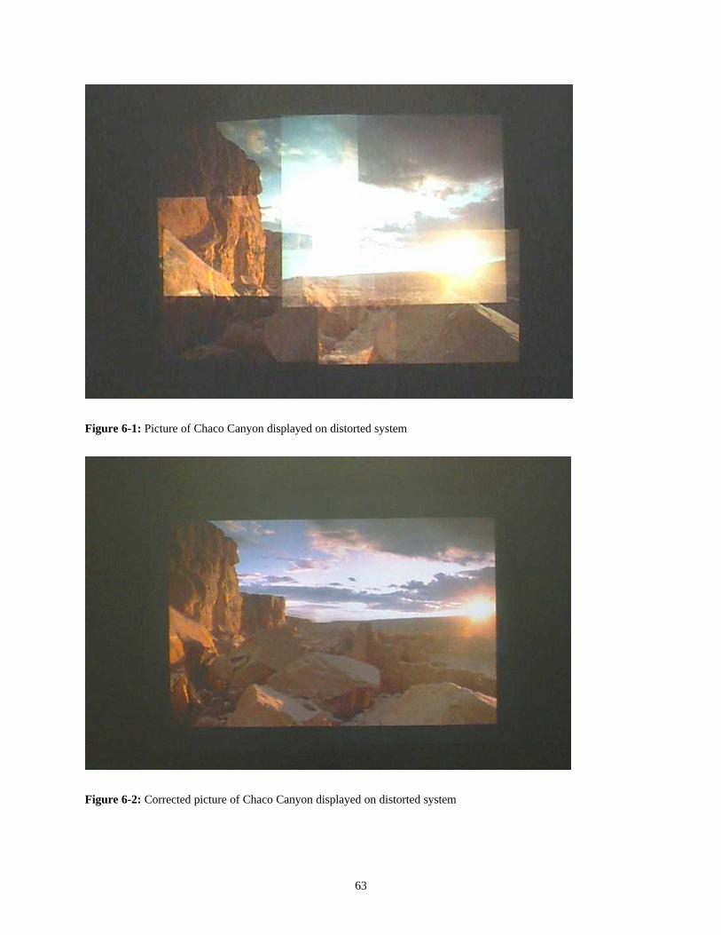
63
Figure 6-1: Picture of Chaco Canyon displayed on distorted system
Figure 6-2: Corrected picture of Chaco Canyon displayed on distorted system

64
Future work While the technology has been shown to work in a small prototype there is much future work.
One area is to make a prototype system that works in real-time. Another area is to make a much
larger prototype system. Below comments relevant comments to both areas of future work will
be given.
Real-time Implementation
The intention in creating these techniques is to build a system that will work in real-time. The
methods discussed in this thesis can be selectively used to create such a system. Assuming that
the system is relatively stable in space such that there is no change in position of the projectors
with respect to the screen, then the positional, and intensity and color warping tables can be
created before the system is used for continuous display. These tables can then be used to
determine the best resolution that can be reconstructed by the system. That resolution can then be
fed back to the computer to be used as the frame-buffer size. The frame buffer must be post-
processed using a hardware accelerator. A hardware accelerator must handle inverse-mapping
back into the frame-buffer, applying the appropriate filtering and finally the color and intensity
mapping to the output pixels. Inverse-mapping is what typical 3-D graphics accelerators do today
when they perform texture mapping. The good graphics accelerators are capable of processing
just under one hundred million pixels per second and using linear interpolation. This suggests
that building hardware that accomplishes the inverse mapping is well within today’s means.
Another nice property is that each graphics card that serves each projector can do these
operations in parallel making it possible to build large-scale systems that work in real time as big
as one wants.
Larger Version of Prototype
The other area that needs to be addressed is the building of a larger prototype. The work that
remains, barring the use of a higher resolution input device, is to compose the input from
multiple cameras viewing the output into a single image. Fortunately, there is a great deal of
work that has all ready been done in this area by researchers seeking a means to higher resolution
input means. The only issue that may come up is properly dealing with the positional intensity
distortion from the different camera lenses, but some of the work that deals with composition
deals with that issue as well.

65
In any case, it seems that all the roadblocks to creating a large-scale version of this display
system that works in real-time are merely in implementation. Hence only time will tell whether it
is a commercial success.
66
Bibliography
[ASP 80] American Society for Photogrammetry, Manual of Photogrammetry, Falls Church,
Va. American Society of Photogrammetry, 1980.
[Babcock 53] H. W. Babcock, Publ. Astron. Soc. Pac, 65, 229, 1953
[Berlin 94] Berlin, Andrew, Towards Intelligent Structures: Active Control of Column Buckling,
Phd Thesis, MIT Department of Electrical Engineering and Computer Science
[Farrell 90] Farrell, Joyce E Fitzhugh, Andrew E. “Discriminability metric based on human
contrast sensitivity, Journal of Optical Society of America A, Volume 7 No, 10 October 1990
pp1976-1984
[Fugate 95] McCullough, P.R., Fugate, R.Q., Christou, J.C., Ellerbroek, B.L., Higgins, C.H.,
Spinhirne, J.M., Cleis, R.A., and Moroney, J.F., "Photoevaporating stellar envelopes observed
with Rayleigh beacon adaptive optics". 1995, ApJ 438, 394-403,
[Haralick 92] Haralick, Robert M. and Shapiro, Linda G. Computer and Robot Vision Reading,
Mass. Addison-Wesley, 1992
[Horn 85] Horn, B. Robot Vision, 1985 MIT Press
[Inova Patent] Inova, Peter. “Seamless Video Display” US Patent #4,974,073
[Lenz 1987] Lenz, R. and Tsai, R. “Techniques for Calibration of the Scale Factor and Image
Center for High Accuracy 3D Machine Vision Metrology” IEEE Journal of Robtoics and
Automation, VOL RA-3, No. 4, August 1987
[Lyon 86] Lyon, P “Edge Blending Multiple Projection Displays on a Dome Surface to Form
Continuous Wide Angle Fields of View” SID Digest 1986
[Lyon 84] Lyon, P and Black S. “A Self-Aligning CRT Projection System with Digital
Correction,” SID Digest 1984
[Robertson 92] Robertson, Alan R. “Color Perception” Physics Todayv 45 n 12 Dec 1, 1992
[Shum 97] Shum, H, Szeliski, “Panoramic Image Mosaics” Microsoft Research Technical Report
MSR-TR-97-23

67
[Smith 90] Smith, Warren Modern Optical Engineering: The Design of Optical Systems
McGraw Hill 1990, New York
[Stumpp 97] Stumpp, Edward H, Projection Displays Short Course, Society for Information
Display Conference
[Tannas 92] Tanna, Lawrence E. Jr. “Color in Electronic Displays” Physics Today v45, Number
12, Dec 1, 1992
[Thorell 90] Thorell, Lisa G. Using Computer Color Effectively: an Illustrated Reference
Prentice Hall, NJ 1990
[Tsai 86] Tsai, Robert “An Efficient and Accurate Camera Calibration Technique for 3D
Machine Vision,” Proceedings of IEEE Conference on Computer Vision and Pattern
Recognition, Miami Beach, FL, 1986, pages 364-374
[Watson 90] Watson, Andrew B. “Perceptual-components architecture for digital video” Journal
of Optical Society of America A, Volume 7 No, 10 October 1990 pp 1943 –1954
[Wandell 95] Wandell, Brian Foundations of Vision, Sinauer Associates, Inc. 1995 Sunderland
Mass
[Wolberg 90] Wolberg, George. Digital Image Warping Ph.D. Thesis 1990 Columbia
University