Scalable Wi-Fi Client Self-Positioning Using Cooperative ...static.tongtianta.site/paper_pdf/1c22188e-9423-11e9-956d-00163e08bb86.pdf · not exposing their presence to the network

This article has been accepted for inclusion in a future issue of this journal. Content is final as presented, with the exception of pagination.

IEEE TRANSACTIONS ON INSTRUMENTATION AND MEASUREMENT 1

Scalable Wi-Fi Client Self-Positioning UsingCooperative FTM-Sensors

Leor Banin, Ofer Bar-Shalom , Nir Dvorecki, and Yuval Amizur

Abstract— This paper presents a protocol that enables anunlimited number of Wi-Fi users to position themselves within ameter-level accuracy and navigate indoors using time-delay-basedWi-Fi measurements. The proposed protocol, called collaborativetime of arrival, is broadcast-based and relies on cooperationbetween the network sensors that support IEEE 802.11 fine-timing measurements (FTMs) capabilities, which are enabled instate-of-the-art Wi-Fi chipsets. The clients can estimate and tracktheir position by passively listening to timing measurements thatare exchanged between the FTM-sensors. The passive nature ofthe clients’ operation enables them to maintain their privacy bynot exposing their presence to the network. This paper outlinesthe principles of the protocol and the mathematical backgroundof the position estimation algorithms. Both theoretical analysisof the expected positioning accuracy, as well as real-life systemperformance examples, are provided. The protocol’s performanceanalysis is based on a publicly available database of real networkmeasurements.

Index Terms— IEEE 802.11 standard, indoor navigation,Kalman filters, maximum-likelihood estimation, multisensor sys-tems, position measurement, time-difference-of-arrival (TDoA),time measurement.

I. INTRODUCTION

RANGING based on time-delay measurements for wire-less local area network (WLAN) 1 mobile devices has

evolved significantly during the past decade. The bandwidthincreases from 20 MHz up to 160 MHz, combined withthe multiple-input-multiple-output (MIMO) technology, hasignited a rapid standardization effort of a fine-timing mea-surement (FTM) protocol [1], [2]. This has facilitated thedevelopment of accurate, time-delay-based Wi-Fi indoor posi-tioning and navigation systems [5]–[14]. FTM is a point-to-point (P2P) single-user protocol, which includes an exchangeof multiple message frames between an initiating Wi-Fi sta-tion (ISTA) and a responding station (RSTA). The ISTA(which is typically a mobile Wi-Fi client such as a mobilephone) attempts to measure its range with respect to theRSTA (e.g., Wi-Fi access point (AP) or a dedicated FTM

Manuscript received August 1, 2018; revised October 21, 2018; acceptedOctober 22, 2018. This work was supported by Intel Communication &Devices Group (iCDG), Intel Corporation. The Associate Editor coor-dinating the review process was Jesús Ureña. (Corresponding author:Ofer Bar-Shalom.)

The authors are with the Intel’s Location Core Division, Petah Tikva 49527,Israel (e-mail: [email protected]).

Color versions of one or more of the figures in this paper are availableonline at http://ieeexplore.ieee.org.

Digital Object Identifier 10.1109/TIM.2018.28808871Commonly referenced using the synonym “Wi-Fi,” which is the Wi-Fi

alliance owned trademark for WLAN technology.

Fig. 1. FTM protocol message flow example.

“responder”). Obtaining an accurate time-delay estimate in adense-multipath environment is challenging and requires anaccurate detection of the first signal path, which is asso-ciated with the line of sight (LoS) between the two sta-tions and estimation of its arrival time. This is implementedusing either superresolution methods [7], [8], or maximum-likelihood methods [9], applied to the estimated channelresponse. The channel response is estimated using train-ing sequences of orthogonal frequency-division multiplexing(OFDM) symbols with known subcarrier modulation includedin the exchanged messages [3]. A schematic description of themessage exchange of the FTM protocol is illustrated in Fig. 1.

The time of flight (ToF) between the two stations is calcu-lated using the following equation:

ToF = (t4 − t1)− (t3 − t2)

2(1)

where t1 denotes the time of departure (ToD) measured bythe RSTA, and t4 denotes the time of arrival (ToA), whichis estimated by the RSTA. The values of t1 and t4 arereported back to the ISTA after the completion of the FTM

0018-9456 © 2018 IEEE. Translations and content mining are permitted for academic research only. Personal use is also permitted,but republication/redistribution requires IEEE permission. See http://www.ieee.org/publications_standards/publications/rights/index.html for more information.

https://orcid.org/0000-0002-1471-2135


2 IEEE TRANSACTIONS ON INSTRUMENTATION AND MEASUREMENT

measurement phase. The values of t1 and t4 are reportedat picosecond granularity using a 48-bit counter that wrapsaround approximately every 281.5 s (= 248 ·10−12). The 48-bitformat was defined mainly to enable a unified timing measure-ment report format for both “millimeter-wave” 802.11 systems(e.g., 60 GHz) and Wi-Fi systems operating in the <7-GHzband. Yet, the achievable timing accuracy for the latter typeis in the order of 1 ns (∼30 cm) [13]. The ISTA combinesthe values of t1 and t4 along with its own estimated ToA (t2)and measured ToD (t3) values, to obtain a range estimate withrespect to the RSTA.2

Being a P2P, single-user protocol, the FTM protocol islimited in scenarios where a large number of users are request-ing positioning services simultaneously. Given that obtaininga single range measurement takes roughly 30-ms per clientstation (cSTA) [16], each AP may only be able to serviceapproximately 30 cSTAs per second (while exhausting itscapacity, leaving it with no bandwidth to provide any dataservices). Moreover, with more and more navigating usersattempting to execute FTM sessions, the likelihood of framecollision increases. This decreases the likelihood of successfulrange measurement, thereby reducing the number of cSTAsthat can be serviced. This is likely to happen in large stadiumshosting rock concerts or major sports events, large airportterminals, central public transportation terminals, and so on.Providing an adequate level of positioning and data servicesto a user capacity of such magnitude would require thedeployment of a network that consists of thousands of FTMresponders. The collaborative ToA (CToA) protocol is aimedto provide a cost-effective solution for such use cases.

CToA is a geolocation protocol designed to provide posi-tioning and navigation services to a large scale of users. Thiscan be achieved using a broadcast approach rather than aP2P or a point to multipoint ranging approach. The proto-col operates over an unmanaged network of unsynchronizedand independent units called “broadcasting stations” (bSTA),which together form a high-precision geolocation network.The bSTAs, deployed at known locations, are implementedusing either standard Wi-Fi APs capable of measuring accurateToA or network detached, responderlike units with FTMcapabilities. According to the protocol [16], the bSTA unitsserve several purposes. Every bSTA:

1) periodically broadcasts CToA “beacons,” which consistof a packet used for timing measurements and some datainformation elements;

2) measures the ToD of its own beacons and announces itwithin the beacon;

3) listens for CToA beacons broadcast by its neighborbSTAs, and measures their ToA;

4) maintains a log of its current ToD and ToA measure-ments and publishes its most recent measurements logas part of its next CToA beacon broadcast; and

5) periodically announces its location as part of its CToAbeacon broadcasts.

2The exchange of the FTM measurement message and its acknowledg-ment (ACK) frame, which has to be sent out after exactly a short interframespacing (SIFS) of 16μs, is assumed to finish within a short period, duringwhich the clocks of the two stations do not drift appreciably.

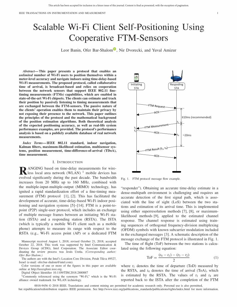
Fig. 2. CToA beacon broadcast example.

The protocol may be visioned as the indoor counterpart ofthe global navigation satellite systems (GNSSs). It is designedfor enabling an unlimited number of clients to estimate theirlocation and navigate while maintaining their privacy. ThecSTAs only passively listen to the bSTA broadcasts. Once acSTA receives a broadcast, it measures its ToA and combinesit with the ToD/ToA measurements log published by the bSTAin their beacons, to determine its current position. Since thecSTAs do not transmit, their presence is unexposed and theirprivacy is maintained.

Fig. 2 illustrates an example of CToA beacon broadcastand its reception. It assumes a CToA network, which consistsof three unsynchronized bSTA units and a single cSTA.These units are assigned with (simplified) medium access con-trol (MAC) addresses: “10:01,” “10:02,” and “10:03,” while thecSTA has a MAC address of “55:55.” As illustrated in Fig. 2,at a time indicated by ToD time-stamp of “199678” (measuredin picoseconds and referenced to the time base of bSTA#1),bSTA#1 broadcasts a CToA beacon associated with packetidentification (PID) “1551.” The ToD and the PID are loggedin a “CToA location measurement report” (CLMR) log-filemaintained by bSTA#1, which also includes the MAC addressof the bSTA. The CLMR broadcast by bSTA1 also includesthe time-stamps it has measured for previous broadcasts itreceived from bSTA#2 and #3. The beacon propagates throughthe channel, and as illustrated in Fig. 2, is received by bSTA#2 & #3, and the cSTA, which update their measurementlogs accordingly: bSTA#2 measured the beacon’s ToA as“329673” (referenced to its own time base) and updates thatvalue in its CLMR log, along with its own MAC address asthe receiving unit. Similarly, bSTA#3 and the cSTA estimateand log the ToAs of that same beacon as “341006,” and“133564,” respectively. The bSTAs also update their CLMRlogs with the additional time-stamps measured by bSTA#1 asreported in its broadcast CLMR. The CLMR is managed asa “sliding-window” of the time-stamps measured during thepast X seconds. The size of that window may be tuned foroptimizing the overall system performance. The entries of theCLMR log table undergo a time-stamp matching phase, during


BANIN & BAR-SHALOM et al.: SCALABLE Wi-Fi CLIENT SELF-POSITIONING USING COOPERATIVE FTM-SENSORS 3

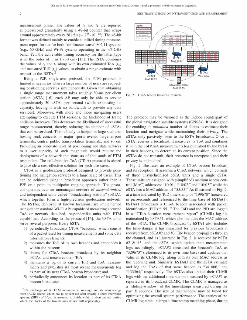
Fig. 3. CToA beacon broadcast timing.

which the ToA measurements are matched with their corre-sponding ToD value. As will be discussed in Section III-B, theclient feeds this timing information, along with the positioninformation of the bSTAs, (also broadcast periodically as partof their beacons), into a Kalman filter that produces an updatedestimate of its current position. The messaging sequence ofthe protocol is described in Fig. 3. The broadcast consistsof two transmitted frames separated by a standard, SIFSof 16 μs [2]. The first frame is called “null-data packet (NDP)announcement” and has a twofold role: it announces the arrivalof the NDP, used by the receiver for measuring the broadcast’sToA, and it conveys the information elements that carry theCLMR and the bSTA location information. A similar broadcastmessaging concept has been discussed in [15], for enablingangular information for the navigating clients. The CToAbeacon duration varies between 100 and 500 μs (dependingon the amount of data contained in the CLMR). Every bSTAbroadcasts a CToA beacon once every 200 to 500 ms. EverybSTA announces its CToA beacon broadcasting schedule tofacilitate the optimization of the cSTAs reception duration.Once the cSTA is tracking its location, it may only wake upfor less than 500 μs every time it wishes to receive a newtiming measurement. The rate, at which the cSTA needs towake up, depends on its required location accuracy and theaccuracy of its crystal oscillator (XO).

A. Related Work and Paper Contributions

The concept of time synchronization for wireless sensor net-works (WSN) using two-way time-stamps exchanges has beenaddressed in [4] (and its referenced sources). The problem ofjoint synchronization and ranging in a WSN between pairs of

nodes exchanging time-stamps has been considered in [12].The localization of a blind node using time-difference-of-arrival (TDoA) measurements enabled by time-stampsexchange has been proposed in [10]. In [11], this solution wasextended for a network-centric architecture, enabling TDoA-based localization and velocity determination of a noncoop-erative node (namely, a node that does not announce theToD of the packets it transmits), using time-stamps exchangedbetween sensor nodes in an asynchronous network. There,the node localization was based on a discrete, least-squares-based fixing, rather than continuous tracking of its positionand network clock parameters. It may be worth noticingthat the solution in [11] is nonscalable in the sense that thenumber of nonoverlapping transmissions, which may be sentby the noncooperative nodes within a given time window,is finite. Furthermore, as the noncooperative nodes transmit,their privacy is compromised.

The contributions of this paper are given in the following.

1) A novel scalable, time-delay-based, client positioningprotocol for unsynchronized Wi-Fi networks.

2) A Kalman filter-based, client positioning engine (PE).3) A theoretical analysis of the PE’s asymptotic accuracy.4) Performance evaluation based on a real indoor network,

for which a measurement database is provided, alongwith the MATLAB source code of the PE (see [17]).

B. Paper Organization

The remainder of this paper is organized as follows.Section II formulates the client position estimation problem.The position estimation algorithms are derived in Section III.This section is divided into two parts; first, Section III-Aoutlines the measurement models and the maximum-likelihoodposition estimators for client mode in the absence of clockdrifts. Then, Section III-B introduces the effect of the clockdrifts on the measurement models and details the Kalmanfilter algorithm executed by the client device and used forestimating and tracking all the time-varying parameters in thesystem. The measurement models derived in Section III-Aare used in Section IV for obtaining bounds on the expectedpositioning accuracy. System-level simulation and real-lifesystem performance are described in Section V. Furtherinsights and design aspects are discussed in Section VI, whilethe final conclusions are summarized in Section VII. Finally,in the Appendix, the Cramér-Rao lower bounds (CRLBs)for the positioning problem are derived. These are used forillustrating the theoretical system performance discussed inSection IV.

Notation: We use lowercase letters to indicate scalars, low-ercase boldface letters to denote vectors, and uppercase bold-face letters to express matrices. Other notations are describednext to their first appearance.

II. PROBLEM FORMULATION

In Section II, the mathematical background of the clientposition estimation is established. Section II-A outlines gen-eral definitions that are used in Section II-B for defining



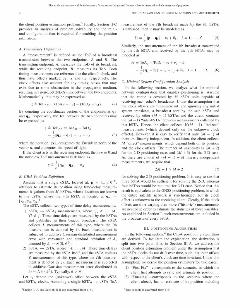
the client position estimation problem.3 Finally, Section II-Cprovides an analysis of problem solvability and the mini-mal configuration that is required for enabling the positionestimation.

A. Preliminary Definitions

A “measurement” is defined as the ToF of a broadcasttransmission between the two endpoints, A and B . Thetransmitting endpoint, A, measures the ToD of its broadcast,while the receiving endpoint, B , measures its ToA. Bothtiming measurements are referenced to the client’s clock, andthus have offsets marked by νA and νB , respectively. Theclock offsets also account for any timing biases that mayexist due to some obstruction in the propagation medium,resulting in a non-LoS (NLoS) link between the two endpoints.Mathematically, this may be expressed as

z � ToFAB = (ToAB + νB)− (ToDA + νA). (2)

By denoting the coordinates vectors of the endpoints as qA

and qB , respectively, the ToF between the two endpoints maybe expressed as

z � ToFAB ≡ ToAB − ToDA

= 1

c�qB − qA� + νB − νA (3)

where the notation, �x�, designates the Euclidean norm of thevector x, and c denotes the speed of light.

If the client acts as the receiving endpoint, then νB ≡ 0 andthe noiseless ToF measurement is defined as

z � 1

c�qB − qA� − νA. (4)

B. CToA Problem Definition

Assume that a single cSTA, located at: p = [x, y, 0]T ,attempts to estimate its position using time-delay measure-ments it gathers from M bSTAs, whose locations are knownto the cSTA, where the mth bSTA is located at qm =[xm, ym, zm ]T .

The cSTA collects two types of time-delay measurements.

1) bSTAi → bSTA j measurements, where i, j ∈ 1 . . .M,∀i �= j . These time delays are measured by the bSTAsand published in their beacon broadcast. The cSTAcollects L measurements of this type, where the lthmeasurement is denoted by zl . Each measurement issubjected to additive Gaussian-distributed measurementerror with zero-mean and standard deviation of σ ,denoted by nl ∼ N (0, σ 2).

2) bSTAi → cSTA, where i ∈ 1 . . .M . These time-delaysare measured by the cSTA itself, and the cSTA collectsL measurements of this type, where the �th measure-ment is denoted by z�. Each measurement is subjectedto additive Gaussian measurement error distributed asn� ∼ N (0, σ 2). Typically, σ > σ .

Let νi denote the (unknown) offset between the cSTAand bSTAi clocks. Assuming a single bSTAi → cSTA ToA

3Section II-A and Section II-B are excerpted from [16].

measurement of the �th broadcast made by the i th bSTA,is unbiased, then it may be modeled as

z� = 1

c�p − qi� − νi + n�, � = 1, . . . ,L. (5)

Similarly, the measurement of the lth broadcast transmittedby the i th bSTA and received by the j th bSTA, may bemodeled as

zl = ToA j − ToDi − νi + ν j + nl

= 1

c�q j − qi� − νi + ν j + nl , l = 1, . . . , L . (6)

C. Minimal System Configuration Analysis

In the following section, we analyze what the minimalnetwork configuration that enables positioning is. Assumethat the venue is covered by M bSTA units capable ofreceiving each other’s broadcasts. Under the assumption thatthe clock offsets are time-invariant, and ignoring any initialsystem transients, a broadcast sent by the mth bSTA andreceived by other (M − 1) bSTAs and the client, containsthe (M −1) “inter-bSTA” previous measurements collected bythat bSTA. Hence, the client collects M(M − 1) “indirect”measurements (which depend only on the unknown clockoffsets). However, it is easy to verify that only (M − 1) ofthem are linearly independent. In addition, the client collectsM “direct” measurements, which depend both on its positionand the clock offsets. The number of unknowns is (M + 2)for the 2-D positioning case, and (M + 3) for the 3-D case.As there are a total of (M − 1) + M linearly independentmeasurements, we require that

2M − 1 ≥ M + 2 (7)

for solving the 2-D positioning problem. It is easy to see thatthree bSTA would be sufficient for solving the 2-D, whereasfour bSTAs would be required for 3-D case. Notice that thisresult is equivalent to the GNSS positioning problem, in whichthe entire satellite network is synchronized, but its clockoffset is unknown to the receiving client. Clearly, if the clockoffsets are time-varying then more (“historic”) measurementsare needed in order to estimate the statistics of these variables.As explained in Section I, such measurements are included inthe broadcasts of every bSTA.

III. POSITIONING ALGORITHMS

In the following section,4 the CToA positioning algorithmsare derived. To facilitate the explanation, the derivation issplit into two parts; first, in Section III-A, we address theclient position estimation problem under the assumption thatthe bSTA clocks do not drift over time, such that their offsetswith respect to the client’s clock are time-invariant. Under thisassumption, we derive the position estimators for two cases.

1) “First-Fix”—corresponds to the scenario, in which theclient first attempts to sync and estimate its position.

2) “Tracking”—corresponds to the scenario where theclient already has an estimate of its position including

4This section is excerpted from [16].



the bSTA timing-related parameters and continues track-ing them using a Kalman filter.

Then, in Section III-B, we outline the Kalman filter thatenables the client to simultaneously estimate and track itsown location coordinates, as well as the clock parameters ofthe bSTAs.

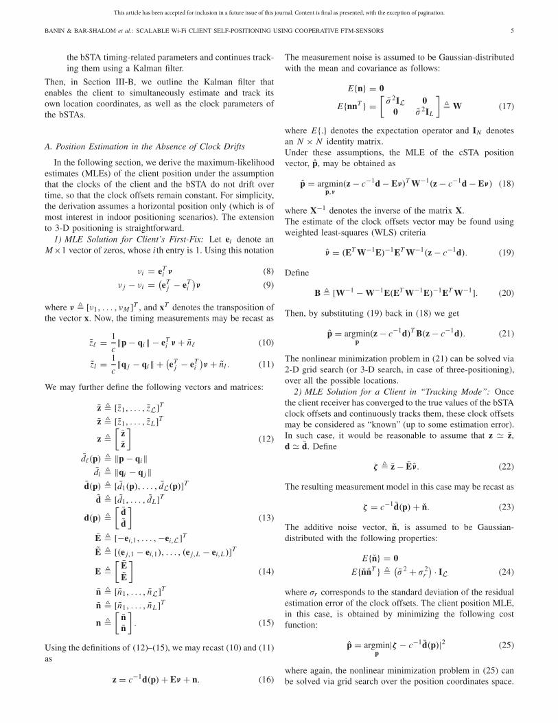
A. Position Estimation in the Absence of Clock Drifts

In the following section, we derive the maximum-likelihoodestimates (MLEs) of the client position under the assumptionthat the clocks of the client and the bSTA do not drift overtime, so that the clock offsets remain constant. For simplicity,the derivation assumes a horizontal position only (which is ofmost interest in indoor positioning scenarios). The extensionto 3-D positioning is straightforward.

1) MLE Solution for Client’s First-Fix: Let ei denote anM×1 vector of zeros, whose i th entry is 1. Using this notation

νi = eTi ν (8)

ν j − νi = (eT

j − eTi

)ν (9)

where ν � [ν1, . . . , νM ]T , and xT denotes the transposition ofthe vector x. Now, the timing measurements may be recast as

z� = 1

c�p − qi� − eT

i ν + n� (10)

zl = 1

c�q j − qi� + (

eTj − eT

i

)ν + nl . (11)

We may further define the following vectors and matrices:z � [z1, . . . , zL]T

z � [z1, . . . , z L ]T

z �[

zz

](12)

d�(p) � �p − qi�dl � �qi − q j�

d(p) � [d1(p), . . . , dL(p)]T

d � [d1, . . . , dL]T

d(p) �[

dd

](13)

E � [−ei,1, . . . ,−ei,L]T

E � [(e j,1 − ei,1), . . . , (e j,L − ei,L )]T

E �[

EE

](14)

n � [n1, . . . , nL]T

n � [n1, . . . , nL ]T

n �[

nn

]. (15)

Using the definitions of (12)–(15), we may recast (10) and (11)as

z = c−1d(p)+ Eν + n. (16)

The measurement noise is assumed to be Gaussian-distributedwith the mean and covariance as follows:

E{n} = 0

E{nnT } =[σ 2IL 0

0 σ 2IL

]� W (17)

where E{.} denotes the expectation operator and IN denotesan N × N identity matrix.Under these assumptions, the MLE of the cSTA positionvector, p, may be obtained as

p = argminp,ν

(z − c−1d − Eν)T W−1(z − c−1d − Eν) (18)

where X−1 denotes the inverse of the matrix X.The estimate of the clock offsets vector may be found usingweighted least-squares (WLS) criteria

ν = (ET W−1E)−1ET W−1(z − c−1d). (19)

Define

B � [W−1 − W−1E(ET W−1E)−1ET W−1]. (20)

Then, by substituting (19) back in (18) we get

p = argminp

(z − c−1d)T B(z − c−1d). (21)

The nonlinear minimization problem in (21) can be solved via2-D grid search (or 3-D search, in case of three-positioning),over all the possible locations.

2) MLE Solution for a Client in “Tracking Mode”: Oncethe client receiver has converged to the true values of the bSTAclock offsets and continuously tracks them, these clock offsetsmay be considered as “known” (up to some estimation error).In such case, it would be reasonable to assume that z z,d d. Define

ζ � z − Eν. (22)

The resulting measurement model in this case may be recast as

ζ = c−1d(p)+ n. (23)

The additive noise vector, n, is assumed to be Gaussian-distributed with the following properties:

E{n} = 0

E{nnT } �(σ 2 + σ 2

r

) · IL (24)

where σr corresponds to the standard deviation of the residualestimation error of the clock offsets. The client position MLE,in this case, is obtained by minimizing the following costfunction:

p = argminp

|ζ − c−1d(p)|2 (25)

where again, the nonlinear minimization problem in (25) canbe solved via grid search over the position coordinates space.



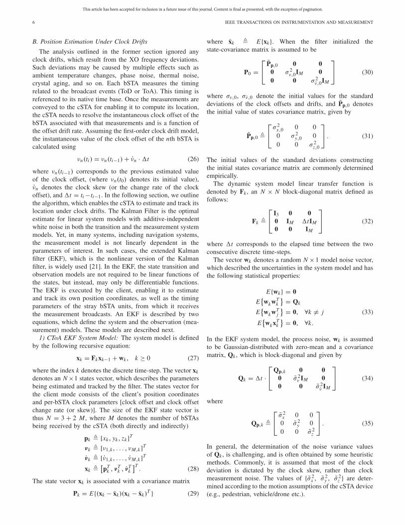
B. Position Estimation Under Clock Drifts

The analysis outlined in the former section ignored anyclock drifts, which result from the XO frequency deviations.Such deviations may be caused by multiple effects such asambient temperature changes, phase noise, thermal noise,crystal aging, and so on. Each bSTA measures the timingrelated to the broadcast events (ToD or ToA). This timing isreferenced to its native time base. Once the measurements areconveyed to the cSTA for enabling it to compute its location,the cSTA needs to resolve the instantaneous clock offset of thebSTA associated with that measurements and is a function ofthe offset drift rate. Assuming the first-order clock drift model,the instantaneous value of the clock offset of the nth bSTA iscalculated using

νn(ti ) = νn(ti−1)+ νn ·�t (26)

where νn(ti−1) corresponds to the previous estimated valueof the clock offset, (where νn(t0) denotes its initial value),νn denotes the clock skew (or the change rate of the clockoffset), and �t = ti −ti−1. In the following section, we outlinethe algorithm, which enables the cSTA to estimate and track itslocation under clock drifts. The Kalman Filter is the optimalestimate for linear system models with additive-independentwhite noise in both the transition and the measurement systemmodels. Yet, in many systems, including navigation systems,the measurement model is not linearly dependent in theparameters of interest. In such cases, the extended Kalmanfilter (EKF), which is the nonlinear version of the Kalmanfilter, is widely used [21]. In the EKF, the state transition andobservation models are not required to be linear functions ofthe states, but instead, may only be differentiable functions.The EKF is executed by the client, enabling it to estimateand track its own position coordinates, as well as the timingparameters of the stray bSTA units, from which it receivesthe measurement broadcasts. An EKF is described by twoequations, which define the system and the observation (mea-surement) models. These models are described next.

1) CToA EKF System Model: The system model is definedby the following recursive equation:

xk = Fkxk−1 + wk, k ≥ 0 (27)

where the index k denotes the discrete time-step. The vector xk

denotes an N ×1 states vector, which describes the parametersbeing estimated and tracked by the filter. The states vector forthe client mode consists of the client’s position coordinatesand per-bSTA clock parameters [clock offset and clock offsetchange rate (or skew)]. The size of the EKF state vector isthus N = 3 + 2 M , where M denotes the number of bSTAsbeing received by the cSTA (both directly and indirectly)

pk � [xk, yk, zk]T

νk � [ν1,k, . . . , νM,k]T

νk � [ν1,k, . . . , νM,k]T

xk �[pT

k , νTk , ν

Tk

]T. (28)

The state vector xk is associated with a covariance matrix

Pk = E{(xk − xk)(xk − xk)T } (29)

where xk � E{xk}. When the filter initialized thestate-covariance matrix is assumed to be

P0 =⎡

⎣Pp,0 0 0

0 σ 2ν,0IM 0

0 0 σ 2ν,0IM

⎤

⎦ (30)

where σν,0, σν,0 denote the initial values for the standarddeviations of the clock offsets and drifts, and Pp,0 denotesthe initial value of states covariance matrix, given by

Pp,0 �

⎡

⎣σ 2

x,0 0 00 σ 2

y,0 00 0 σ 2

z,0

⎤

⎦ . (31)

The initial values of the standard deviations constructingthe initial states covariance matrix are commonly determinedempirically.

The dynamic system model linear transfer function isdenoted by Fk , an N × N block-diagonal matrix defined asfollows:

Fk �

⎡

⎣I3 0 00 IM �tIM

0 0 IM

⎤

⎦ (32)

where �t corresponds to the elapsed time between the twoconsecutive discrete time-steps.

The vector wk denotes a random N ×1 model noise vector,which described the uncertainties in the system model and hasthe following statistical properties:

E{wk} = 0

E{wkwT

k

} = Qk

E{wkwT

j

} = 0, ∀k �= j (33)

E{wkxT

k

} = 0, ∀k.

In the EKF system model, the process noise, wk is assumedto be Gaussian-distributed with zero-mean and a covariancematrix, Qk , which is block-diagonal and given by

Qk = �t ·⎡

⎣Qp,k 0 0

0 σ 2ν IM 0

0 0 σ 2ν IM

⎤

⎦ (34)

where

Qp,k �

⎡

⎣σ 2

x 0 00 σ 2

y 00 0 σ 2

z

⎤

⎦ . (35)

In general, the determination of the noise variance valuesof Qk , is challenging, and is often obtained by some heuristicmethods. Commonly, it is assumed that most of the clockdeviation is dictated by the clock skew, rather than clockmeasurement noise. The values of {σ 2

x , σ2y , σ

2z } are deter-

mined according to the motion assumptions of the cSTA device(e.g., pedestrian, vehicle/drone etc.).



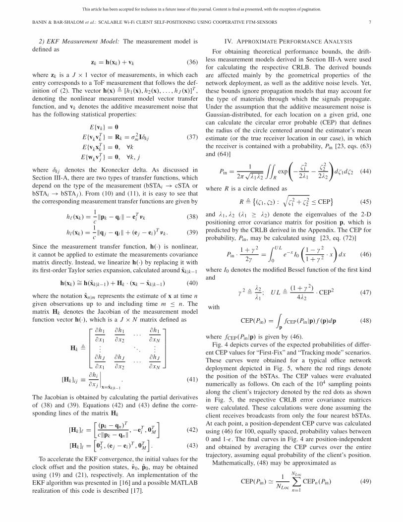
2) EKF Measurement Model: The measurement model isdefined as

zk = h(xk)+ vk (36)

where zk is a J × 1 vector of measurements, in which eachentry corresponds to a ToF measurement that follows the def-inition of (2). The vector h(x) � [h1(x), h2(x), . . . , h J (x)]T ,denoting the nonlinear measurement model vector transferfunction, and vk denotes the additive measurement noise thathas the following statistical properties:

E{vk} = 0

E{vkvTk } = Rk = σ 2

mIδkj (37)

E{vkxTk } = 0, ∀k

E{wkvTj } = 0, ∀k, j

where δkj denotes the Kronecker delta. As discussed inSection III-A, there are two types of transfer functions, whichdepend on the type of the measurement (bSTAi → cSTA orbSTAi → bSTA j ). From (10) and (11), it is easy to see thatthe corresponding measurement transfer functions are given by

h�(xk) = 1

c�pk − qi� − eT

i νk (38)

hl(xk) = 1

c�q j − qi� + (e j − ei )

T νk . (39)

Since the measurement transfer function, h(·) is nonlinear,it cannot be applied to estimate the measurements covariancematrix directly. Instead, we linearize h(·) by replacing it withits first-order Taylor series expansion, calculated around xk|k−1

h(xk) ∼= h(xk|k−1)+ Hk · (xk − xk|k−1) (40)

where the notation xn|m represents the estimate of x at time ngiven observations up to and including time m ≤ n. Thematrix Hk denotes the Jacobian of the measurement modelfunction vector h(·), which is a J × N matrix defined as

Hk �

⎡

⎢⎢⎢⎢⎣

∂h1

∂x1

∂h1

∂x2· · · ∂h1

∂xN...

. . ....

∂h J

∂x1

∂h J

∂x2· · · ∂h J

∂xN

⎤

⎥⎥⎥⎥⎦

[Hk]i j ≡ ∂hi

∂x j

∣∣∣∣x=xk|k−1

. (41)

The Jacobian is obtained by calculating the partial derivativesof (38) and (39). Equations (42) and (43) define the corre-sponding lines of the matrix Hk

[Hk]� =[(pk − qn)

T

c�pk − qn� ,−eTi , 0T

M

](42)

[Hk]l =[0T

3 , (e j − ei )T , 0T

M

]. (43)

To accelerate the EKF convergence, the initial values for theclock offset and the position states, ν0, p0, may be obtainedusing (19) and (21), respectively. An implementation of theEKF algorithm was presented in [16] and a possible MATLABrealization of this code is described [17].

IV. APPROXIMATE PERFORMANCE ANALYSIS

For obtaining theoretical performance bounds, the drift-less measurement models derived in Section III-A were usedfor calculating the respective CRLB. The derived boundsare affected mainly by the geometrical properties of thenetwork deployment, as well as the additive noise levels. Yet,these bounds ignore propagation models that may account forthe type of materials through which the signals propagate.Under the assumption that the additive measurement noise isGaussian-distributed, for each location on a given grid, onecan calculate the circular error probable (CEP) that definesthe radius of the circle centered around the estimator’s meanestimate (or the true receiver location in our case), in whichthe receiver is contained with a probability, Pin [23, eqs. (63)and (64)]

Pin = 1

2π√λ1λ2

∫∫

Rexp

(

− ζ 21

2λ1− ζ 2

2

2λ2

)

dζ1dζ2 (44)

where R is a circle defined as

R �{(ζ1, ζ2) :

√ζ 2

1 + ζ 22 ≤ CEP

}(45)

and λ1, λ2 (λ1 ≥ λ2) denote the eigenvalues of the 2-Dpositioning error covariance matrix for position p, which ispredicted by the CRLB derived in the Appendix. The CEP forprobability, Pin, may be calculated using [23, eq. (72)]

Pin · 1 + γ 2

2γ=∫ U L

0e−x I0

(1 − γ 2

1 + γ 2 · x

)dx (46)

where I0 denotes the modified Bessel function of the first kindand

γ 2 � λ2

λ1; U L � (1 + γ 2)

4λ2· CEP2 (47)

with

CEP(Pin) =∫

pfCEP(Pin|p) f (p)dp (48)

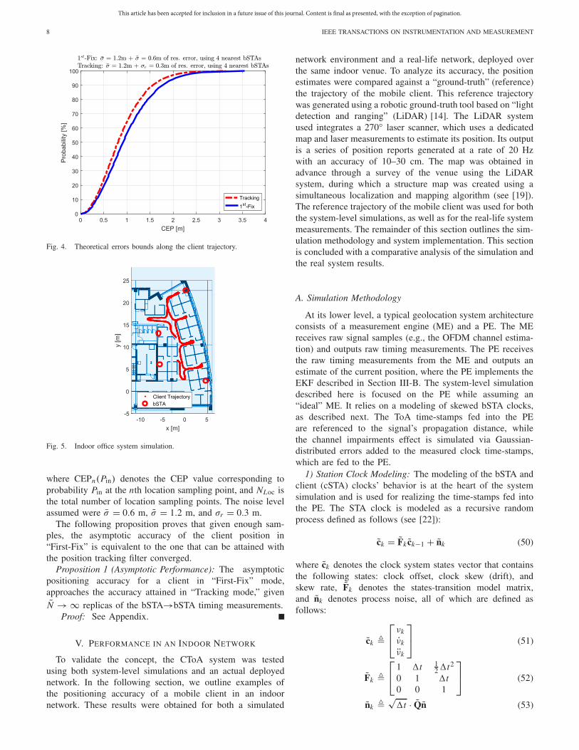
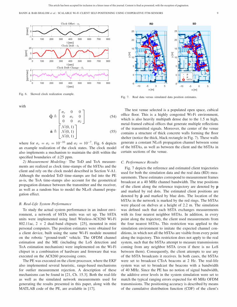
where fCEP(Pin|p) is given by (46).Fig. 4 depicts curves of the expected probabilities of differ-

ent CEP values for “First-Fix” and “Tracking mode” scenarios.These curves were obtained for a typical office networkdeployment depicted in Fig. 5, where the red rings denotethe position of the bSTAs. The CEP values were evaluatednumerically as follows. On each of the 104 sampling pointsalong the client’s trajectory denoted by the red dots as shownin Fig. 5, the respective CRLB error covariance matriceswere calculated. These calculations were done assuming theclient receives broadcasts from only the four nearest bSTAs.At each point, a position-dependent CEP curve was calculatedusing (46) for 100, equally spaced, probability values between0 and 1-�. The final curves in Fig. 4 are position-independentand obtained by averaging the CEP curves over the entiretrajectory, assuming equal probability of the client’s position.

Mathematically, (48) may be approximated as

CEP(Pin) 1

NLoc

NLoc∑

n=1

CEPn(Pin) (49)



Fig. 4. Theoretical errors bounds along the client trajectory.

Fig. 5. Indoor office system simulation.

where CEPn(Pin) denotes the CEP value corresponding toprobability Pin at the nth location sampling point, and NLoc isthe total number of location sampling points. The noise levelassumed were σ = 0.6 m, σ = 1.2 m, and σr = 0.3 m.

The following proposition proves that given enough sam-ples, the asymptotic accuracy of the client position in“First-Fix” is equivalent to the one that can be attained withthe position tracking filter converged.

Proposition 1 (Asymptotic Performance): The asymptoticpositioning accuracy for a client in “First-Fix” mode,approaches the accuracy attained in “Tracking mode,” given

N → ∞ replicas of the bSTA→bSTA timing measurements.Proof: See Appendix.

V. PERFORMANCE IN AN INDOOR NETWORK

To validate the concept, the CToA system was testedusing both system-level simulations and an actual deployednetwork. In the following section, we outline examples ofthe positioning accuracy of a mobile client in an indoornetwork. These results were obtained for both a simulated

network environment and a real-life network, deployed overthe same indoor venue. To analyze its accuracy, the positionestimates were compared against a “ground-truth” (reference)the trajectory of the mobile client. This reference trajectorywas generated using a robotic ground-truth tool based on “lightdetection and ranging” (LiDAR) [14]. The LiDAR systemused integrates a 270◦ laser scanner, which uses a dedicatedmap and laser measurements to estimate its position. Its outputis a series of position reports generated at a rate of 20 Hzwith an accuracy of 10–30 cm. The map was obtained inadvance through a survey of the venue using the LiDARsystem, during which a structure map was created using asimultaneous localization and mapping algorithm (see [19]).The reference trajectory of the mobile client was used for boththe system-level simulations, as well as for the real-life systemmeasurements. The remainder of this section outlines the sim-ulation methodology and system implementation. This sectionis concluded with a comparative analysis of the simulation andthe real system results.

A. Simulation Methodology

At its lower level, a typical geolocation system architectureconsists of a measurement engine (ME) and a PE. The MEreceives raw signal samples (e.g., the OFDM channel estima-tion) and outputs raw timing measurements. The PE receivesthe raw timing measurements from the ME and outputs anestimate of the current position, where the PE implements theEKF described in Section III-B. The system-level simulationdescribed here is focused on the PE while assuming an“ideal” ME. It relies on a modeling of skewed bSTA clocks,as described next. The ToA time-stamps fed into the PEare referenced to the signal’s propagation distance, whilethe channel impairments effect is simulated via Gaussian-distributed errors added to the measured clock time-stamps,which are fed to the PE.

1) Station Clock Modeling: The modeling of the bSTA andclient (cSTA) clocks’ behavior is at the heart of the systemsimulation and is used for realizing the time-stamps fed intothe PE. The STA clock is modeled as a recursive randomprocess defined as follows (see [22]):

ck = Fk ck−1 + nk (50)

where ck denotes the clock system states vector that containsthe following states: clock offset, clock skew (drift), andskew rate, Fk denotes the states-transition model matrix,and nk denotes process noise, all of which are defined asfollows:

ck �

⎡

⎣νk

νk

νk

⎤

⎦ (51)

Fk �

⎡

⎣1 �t 1

2�t2

0 1 �t0 0 1

⎤

⎦ (52)

nk �√�t · Qn (53)



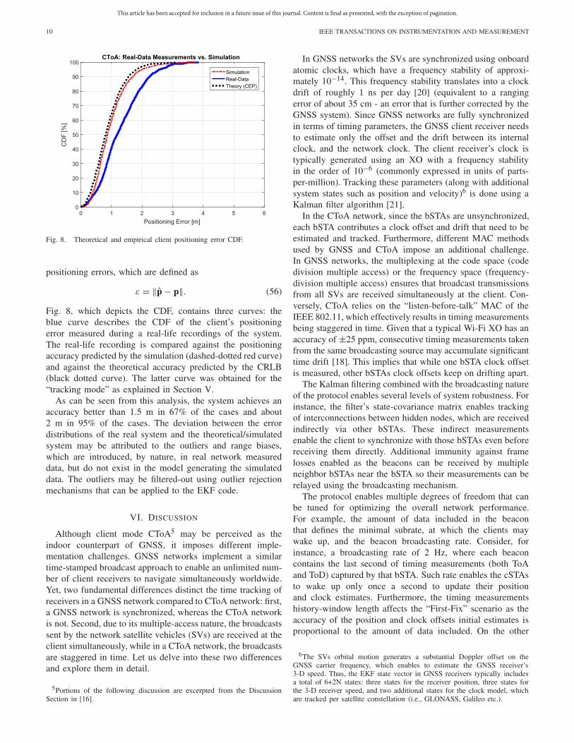
Fig. 6. Skewed clock realization example.

with

Q �

⎡

⎣σν 0 00 σν 00 0 σν

⎤

⎦ (54)

n �

⎡

⎣N (0, 1)N (0, 1)N (0, 1)

⎤

⎦ (55)

where for σν = σν = 10−10 and σν = 10−7. Fig. 6 depictsan example realization of the clock states. The clock modelalso implements a mechanism to maintain the drift within thespecified boundaries of ±25 ppm.

2) Measurement Modeling: The ToD and ToA measure-ments are realized as clock time-stamps of the bSTAs and theclient and rely on the clock model described in Section V-A1.Although the modeled ToD time-stamps are fed into the PEas-is, the ToA time-stamps also account for the geometricalpropagation distance between the transmitter and the receiver,as well as a random bias to model the NLoS channel propa-gation effect.

B. Real-Life System Performance

To study the actual system performance in an indoor envi-ronment, a network of bSTA units was set up. The bSTAunits were implemented using Intel Wireless-AC8260 Wi-Fi802.11ac, 2 × 2 dual-band chipsets [25], mounted in minipersonal computers. The position estimates were obtained fora client device, built using the same Wi-Fi module mountedon the robotic “ground-truth” vehicle. The OFDM channelestimation and the ME (including the LoS detection andToA estimation mechanism) were implemented on the Wi-Fichipset in a combination of hardware and firmware that wasexecuted on the AC8260 processing cores.

The PE was executed on the client processor, where the EKFalso implemented several heuristic, range-based mechanismsfor outlier measurement rejection. A description of thesemechanisms can be found in [21, Ch. 15.3]. Both the real-lifeas well as the simulated network measurements used forgenerating the results presented in this paper, along with theMATLAB code of the PE, are available in [17].

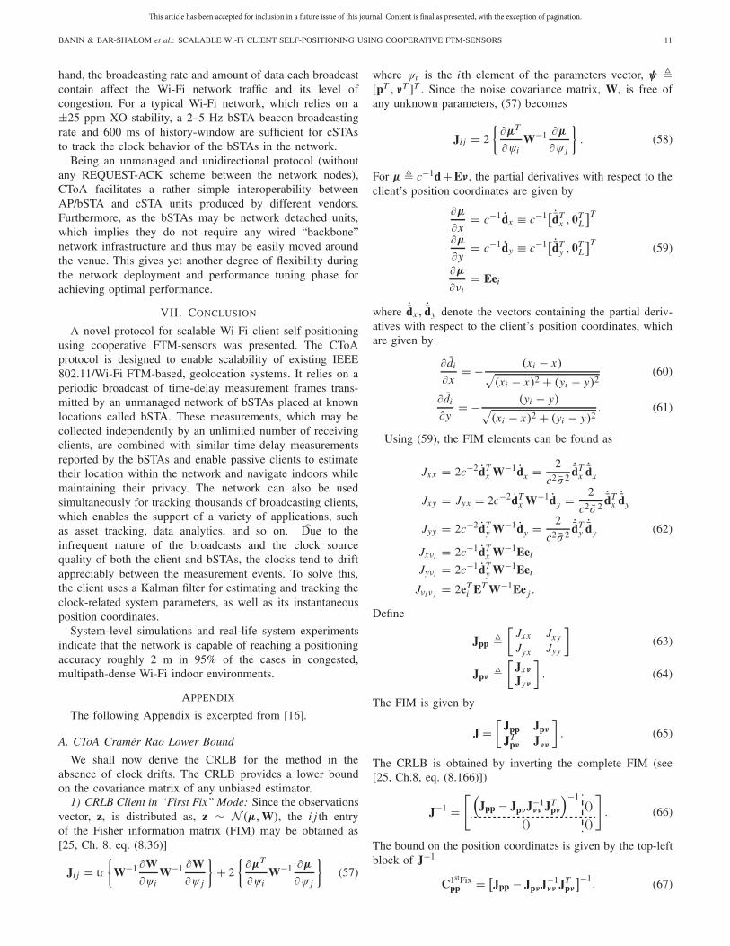
Fig. 7. Real data versus simulated data position estimates.

The test venue selected is a populated open space, cubicaloffice floor. This is a highly congested Wi-Fi environment,which is also heavily multipath dense due to the 1.5 m high,metal-framed cubical offices that generate multiple reflectionsof the transmitted signals. Moreover, the center of the venuecontains a structure of thick concrete walls forming the floorshelter (notice the thick, black rectangle in Fig. 7). These wallsgenerate a constant NLoS propagation channel between someof the bSTAs, as well as between the client and the bSTAs incertain sections of the venue.

C. Performance Results

Fig. 7 depicts the reference and estimated client trajectoriesused for both the simulation data and the real data (RD) mea-surements. These estimates correspond to measurement framesbroadcast at a 40 MHz channel bandwidth. The true positionsof the client along the reference trajectory are denoted by pand marked by red dots. The estimated client positions aredenoted by p and marked by blue dots. The location of thebSTAs in the network is marked by the red rings. The bSTAswere placed on shelves at a height of 2.2 m. The simulationwas defined such that each bSTA exchanges measurementswith its four nearest neighbor bSTAs. In addition, in everypoint along the trajectory, the client used measurements fromthe four nearest bSTAs. This restriction was applied to thesimulation environment to imitate the expected channel con-ditions, in which not all the bSTAs are visible from every pointalong the trajectory. This restriction does not apply to the realsystem, such that the bSTAs attempt to measure transmissionscoming from any neighbor bSTA (even if there is no LoSbetween them). Consequently, the client attempts to use anyof the bSTA broadcasts it receives. In both cases, the bSTAswere set to broadcast CToA beacons at 2 Hz. The real-lifesystem was set to broadcast the beacons with a bandwidthof 40 MHz. Since the PE has no notion of signal bandwidth,the additive error levels in the system simulation were set tomatch the typical ranging errors expected for 40 MHz OFDMtransmissions. The positioning accuracy is described by meansof the cumulative distribution function (CDF) of the client’s



Fig. 8. Theoretical and empirical client positioning error CDF.

positioning errors, which are defined as

ε = �p − p�. (56)

Fig. 8, which depicts the CDF, contains three curves: theblue curve describes the CDF of the client’s positioningerror measured during a real-life recordings of the system.The real-life recording is compared against the positioningaccuracy predicted by the simulation (dashed-dotted red curve)and against the theoretical accuracy predicted by the CRLB(black dotted curve). The latter curve was obtained for the“tracking mode” as explained in Section V.

As can be seen from this analysis, the system achieves anaccuracy better than 1.5 m in 67% of the cases and about2 m in 95% of the cases. The deviation between the errordistributions of the real system and the theoretical/simulatedsystem may be attributed to the outliers and range biases,which are introduced, by nature, in real network measureddata, but do not exist in the model generating the simulateddata. The outliers may be filtered-out using outlier rejectionmechanisms that can be applied to the EKF code.

VI. DISCUSSION

Although client mode CToA5 may be perceived as theindoor counterpart of GNSS, it imposes different imple-mentation challenges. GNSS networks implement a similartime-stamped broadcast approach to enable an unlimited num-ber of client receivers to navigate simultaneously worldwide.Yet, two fundamental differences distinct the time tracking ofreceivers in a GNSS network compared to CToA network: first,a GNSS network is synchronized, whereas the CToA networkis not. Second, due to its multiple-access nature, the broadcastssent by the network satellite vehicles (SVs) are received at theclient simultaneously, while in a CToA network, the broadcastsare staggered in time. Let us delve into these two differencesand explore them in detail.

5Portions of the following discussion are excerpted from the DiscussionSection in [16].

In GNSS networks the SVs are synchronized using onboardatomic clocks, which have a frequency stability of approxi-mately 10−14. This frequency stability translates into a clockdrift of roughly 1 ns per day [20] (equivalent to a rangingerror of about 35 cm - an error that is further corrected by theGNSS system). Since GNSS networks are fully synchronizedin terms of timing parameters, the GNSS client receiver needsto estimate only the offset and the drift between its internalclock, and the network clock. The client receiver’s clock istypically generated using an XO with a frequency stabilityin the order of 10−6 (commonly expressed in units of parts-per-million). Tracking these parameters (along with additionalsystem states such as position and velocity)6 is done using aKalman filter algorithm [21].

In the CToA network, since the bSTAs are unsynchronized,each bSTA contributes a clock offset and drift that need to beestimated and tracked. Furthermore, different MAC methodsused by GNSS and CToA impose an additional challenge.In GNSS networks, the multiplexing at the code space (codedivision multiple access) or the frequency space (frequency-division multiple access) ensures that broadcast transmissionsfrom all SVs are received simultaneously at the client. Con-versely, CToA relies on the “listen-before-talk” MAC of theIEEE 802.11, which effectively results in timing measurementsbeing staggered in time. Given that a typical Wi-Fi XO has anaccuracy of ±25 ppm, consecutive timing measurements takenfrom the same broadcasting source may accumulate significanttime drift [18]. This implies that while one bSTA clock offsetis measured, other bSTAs clock offsets keep on drifting apart.

The Kalman filtering combined with the broadcasting natureof the protocol enables several levels of system robustness. Forinstance, the filter’s state-covariance matrix enables trackingof interconnections between hidden nodes, which are receivedindirectly via other bSTAs. These indirect measurementsenable the client to synchronize with those bSTAs even beforereceiving them directly. Additional immunity against framelosses enabled as the beacons can be received by multipleneighbor bSTAs near the bSTA so their measurements can berelayed using the broadcasting mechanism.

The protocol enables multiple degrees of freedom that canbe tuned for optimizing the overall network performance.For example, the amount of data included in the beaconthat defines the minimal subrate, at which the clients maywake up, and the beacon broadcasting rate. Consider, forinstance, a broadcasting rate of 2 Hz, where each beaconcontains the last second of timing measurements (both ToAand ToD) captured by that bSTA. Such rate enables the cSTAsto wake up only once a second to update their positionand clock estimates. Furthermore, the timing measurementshistory-window length affects the “First-Fix” scenario as theaccuracy of the position and clock offsets initial estimates isproportional to the amount of data included. On the other

6The SVs orbital motion generates a substantial Doppler offset on theGNSS carrier frequency, which enables to estimate the GNSS receiver’s3-D speed. Thus, the EKF state vector in GNSS receivers typically includesa total of 6+2N states: three states for the receiver position, three states forthe 3-D receiver speed, and two additional states for the clock model, whichare tracked per satellite constellation (i.e., GLONASS, Galileo etc.).



hand, the broadcasting rate and amount of data each broadcastcontain affect the Wi-Fi network traffic and its level ofcongestion. For a typical Wi-Fi network, which relies on a±25 ppm XO stability, a 2–5 Hz bSTA beacon broadcastingrate and 600 ms of history-window are sufficient for cSTAsto track the clock behavior of the bSTAs in the network.

Being an unmanaged and unidirectional protocol (withoutany REQUEST-ACK scheme between the network nodes),CToA facilitates a rather simple interoperability betweenAP/bSTA and cSTA units produced by different vendors.Furthermore, as the bSTAs may be network detached units,which implies they do not require any wired “backbone”network infrastructure and thus may be easily moved aroundthe venue. This gives yet another degree of flexibility duringthe network deployment and performance tuning phase forachieving optimal performance.

VII. CONCLUSION

A novel protocol for scalable Wi-Fi client self-positioningusing cooperative FTM-sensors was presented. The CToAprotocol is designed to enable scalability of existing IEEE802.11/Wi-Fi FTM-based, geolocation systems. It relies on aperiodic broadcast of time-delay measurement frames trans-mitted by an unmanaged network of bSTAs placed at knownlocations called bSTA. These measurements, which may becollected independently by an unlimited number of receivingclients, are combined with similar time-delay measurementsreported by the bSTAs and enable passive clients to estimatetheir location within the network and navigate indoors whilemaintaining their privacy. The network can also be usedsimultaneously for tracking thousands of broadcasting clients,which enables the support of a variety of applications, suchas asset tracking, data analytics, and so on. �Due to theinfrequent nature of the broadcasts and the clock sourcequality of both the client and bSTAs, the clocks tend to driftappreciably between the measurement events. To solve this,the client uses a Kalman filter for estimating and tracking theclock-related system parameters, as well as its instantaneousposition coordinates.

System-level simulations and real-life system experimentsindicate that the network is capable of reaching a positioningaccuracy roughly 2 m in 95% of the cases in congested,multipath-dense Wi-Fi indoor environments.

APPENDIX

The following Appendix is excerpted from [16].

A. CToA Cramér Rao Lower Bound

We shall now derive the CRLB for the method in theabsence of clock drifts. The CRLB provides a lower boundon the covariance matrix of any unbiased estimator.

1) CRLB Client in “First Fix” Mode: Since the observationsvector, z, is distributed as, z ∼ N (μ,W), the i j th entryof the Fisher information matrix (FIM) may be obtained as[25, Ch. 8, eq. (8.36)]

Ji j = tr

{W−1 ∂W

∂ψiW−1 ∂W

∂ψ j

}+ 2

{∂μT

∂ψiW−1 ∂μ

∂ψ j

}(57)

where ψi is the i th element of the parameters vector, ψ �[pT , νT ]T . Since the noise covariance matrix, W, is free ofany unknown parameters, (57) becomes

Ji j = 2

{∂μT

∂ψiW−1 ∂μ

∂ψ j

}. (58)

For μ � c−1d + Eν , the partial derivatives with respect to theclient’s position coordinates are given by

∂μ

∂x= c−1dx ≡ c−1[ ˙dT

x , 0TL

]T

∂μ

∂y= c−1dy ≡ c−1[ ˙dT

y , 0TL

]T (59)

∂μ

∂νi= Eei

where ˙dx ,˙dy denote the vectors containing the partial deriv-

atives with respect to the client’s position coordinates, whichare given by

∂ di

∂x= − (xi − x)

√(xi − x)2 + (yi − y)2

(60)

∂ di

∂y= − (yi − y)

√(xi − x)2 + (yi − y)2

. (61)

Using (59), the FIM elements can be found as

Jx x = 2c−2dTx W−1dx = 2

c2σ 2˙dT

x˙dx

Jxy = Jyx = 2c−2dTx W−1dy = 2

c2σ 2˙dT

x˙dy

Jyy = 2c−2dTy W−1dy = 2

c2σ 2˙dT

y˙dy (62)

Jxνi = 2c−1dTx W−1Eei

Jyνi = 2c−1dTy W−1Eei

Jνi ν j = 2eTi ET W−1Ee j .

Define

Jpp �[

Jx x JxyJyx Jyy

](63)

Jpν �[

Jxν

Jyν

]. (64)

The FIM is given by

J =[

Jpp JpνJT

pν Jνν

]. (65)

The CRLB is obtained by inverting the complete FIM (see[25, Ch.8, eq. (8.166)])

J−1 =[(

Jpp − JpνJ−1νν JT

pν

)−1()

() ()

]

. (66)

The bound on the position coordinates is given by the top-leftblock of J−1

C1stFixpp = [


pν]−1

. (67)



2) Approximate CRLB for a Client in “Tracking Mode”:When the EKF is converged and the bSTA clock offsets areknown (up to some residual error), and are being continuouslytracked, then μ c−1d, and ψ � p.

Consequently

Ji j 2

c2(σ 2 + σ 2r )

{∂μT

∂ψi

∂μ

∂ψ j

}. (68)

The partial derivatives are obtained using (59), and the CRLBon the position coordinates estimation error is obtained by

CTrackingpp 1

Jx x Jyy − J 2xy

[Jyy −Jxy

−Jxy Jx x

]

=[σ 2

x x σxyσxy σ 2

yy

]. (69)

B. Proof of Proposition 1

Assume that every broadcast includes N replicas of thetiming measurements collected by the bSTA. Recall that Ldenotes the number of broadcast timing measurements thatwere measured by the client itself, then if the clock offsetswere time-invariant then one could define

E �[

E1N ⊗ E

], W �

[σ 2IL 0

0 σ 2IN×L

]. (70)

Next, from (62), we have

Jνiν j = 2eTi ET W−1Ee j . (71)

Then, under (70), Jνi ν j becomes

Jνiν j = 2eTi ET W−1Ee j

= 2eTi

[σ−2ET σ−21T

N⊗ ET

] [ E1N ⊗ E

]Ee j

= 2eTi (σ

−2ET E + N · σ−2ET E)e j

≈N→∞

2N σ−2eTi EET e j . (72)

Recall that from (67), we have

C1stFixpp = [


pν]−1

. (73)

Hence, under N → ∞, Jpν J−1νν JT

pν → 0.Thus, given enough bSTA→bSTA measurements (equivalentto an EKF in “Tracking mode”), C1stFix

pp ≈ CTrackingpp (up to

additive noise level scaling).This concludes the proof.

ACKNOWLEDGMENT

An earlier version of this paper has been presentedas a whitepaper during the September 2017 meeting ofIEEE 802.11 TGaz in Waikoloa, HI (see [16]). Specifically,Sections II-A and II-B, the great majority of Section III, mostof the discussion in Section VI, and the Appendix have beenreused from that whitepaper.

REFERENCES

[1] E. Au, “The latest progress on IEEE 802.11mc and IEEE 802.11ai[standards],” IEEE Veh. Technol. Mag., vol. 11, no. 3, pp. 19–21,Sep. 2016.

[2] IEEE Standard for Information Technology–Telecommunications andInformation Exchange Between Systems Local and Metropolitan AreaNetworks–Specific Requirements—Part 11: Wireless LAN MediumAccess Control (MAC) and Physical Layer (PHY) Specifications, IEEEStandard 802.11-2016, 2016.

[3] E. Perahia and R. Stacey, Next Generation Wireless LANs: 802.11n and802.11ac, 2nd Ed. Cambridge, U.K.: Cambridge Univ. Press, 2013.

[4] B. Sundararaman, U. Buy, and A. D. Kshemkalyani, “Clock synchro-nization for wireless sensor networks: A survey,” Ad Hoc Netw., vol. 3,no. 3, pp. 281–323, 2005.

[5] A. Makki, A. Siddig, and C. J. Bleakley, “Robust high resolution timeof arrival estimation for indoor WLAN ranging,” IEEE Trans. Instrum.Meas., vol. 66, no. 10, pp. 2703–2710, Oct. 2017.

[6] P. Serrano, P. Salvador, V. Mancuso, and Y. Grunenberger, “Experi-menting with commodity 802.11 hardware: Overview and future direc-tions,” IEEE Commun. Surveys Tuts., vol. 17, no. 2, pp. 671–699,2nd Quart., 2015.

[7] X. Li and K. Pahlavan, “Super-resolution TOA estimation with diversityfor indoor geolocation,” IEEE Trans. Wireless Commun., vol. 3, no. 1,pp. 224–234, Jan. 2004.

[8] F. X. Ge, D. Shen, Y. Peng, and V. O. K. Li, “Super-resolution timedelay estimation in multipath environments,” IEEE Trans. Circuits Syst.I, Reg. Papers, vol. 54, no. 9, pp. 1977–1986, Sep. 2007.

[9] P. J. Voltz and D. Hernandez, “Maximum likelihood time of arrivalestimation for real-time physical location tracking of 802.11a/g mobilestations in indoor environments,” in Proc. IEEE Position LocationNavigat. Symp. (PLANS), Apr. 2004, pp. 585–591.

[10] F. Bandiera, A. Coluccia, G. Ricci, F. Ricciato, and D. Spano, “TDOAlocalization in asynchronous WSNs,” in Proc. 12th IEEE Int. Conf.Embedded Ubiquitous Comput., Milano, Italy, Aug. 2014, pp. 193–196.

[11] F. Ricciato, S. Sciancalepore, F. Gringoli, N. Facchi, and G. Boggia,“Position and velocity estimation of a non-cooperative source fromasynchronous packet arrival time measurements,” IEEE Trans. MobileComput., vol. 17, no. 9, pp. 2166–2179, Sep. 2018.

[12] R. T. Rajan and A. J. V. D. Veen, “Joint ranging and synchronization foran anchorless network of mobile nodes,” IEEE Trans. Signal Process.,vol. 63, no. 8, pp. 1925–1940, Apr. 2015.

[13] L. Banin, U. Schatzberg, and Y. Amizur, “Next generation indoorpositioning system based on WiFi time of flight,” in Proc. 26th Int. Tech.Meeting Satellite Division Inst. Navigat., Nashville TN, USA, Sep. 2013,pp. 975–982.

[14] L. Banin, U. Schatzberg, and Y. Amizur, “WiFi FTM and mapinformation fusion for accurate positioning,” in Proc. Int. Conf. IndoorPositioning Indoor Navigat. (IPIN), Alcalá de Henares, Spain, Oct. 2016.[Online]. Available: http://www3.uah.es/ipin2016/usb/app/descargas/215_WIP.pdf

[15] N. Dvorecki, O. Bar-Shalom, and Y. Amizur, “AoD-based positioningfor Wi-Fi OFDM receivers,” in Proc. 30th Int. Tech. Meeting SatelliteDivision Inst. Navigat. (ION GNSS), Portland, OR, USA, Sep. 2017,pp. 2883–2893.

[16] L. Banin, O. Bar-Shalom, N. Dvorecki, and Y. Amizur, High-AccuracyIndoor Geolocation Using Collaborative Time of Arrival(CToA)—Whitepaper, document IEEE 802.11-17/1387R0, Sep. 2017.[Online]. Available: https://mentor.ieee.org/802.11/dcn/17/11-17-1387-00-00az-high-accuracy-indoor-geolocation-using-collaborative-time-of-arrival-ctoa-whitepaper.pdf

[17] L. Banin, O. Bar-Shalom, N. Dvorecki, and Y. Amizur. Reference-PE-and-Measurements-DB-for-WiFi-Time-Based-Scalable-Location. Acces-sed: Apr. 2018. [Online]. Available: https://github.com/intel/Reference-PE-and-Measurements-DB-for-WiFi-Time-based-Scalable-Location

[18] H. Kim, X. Ma, and B. R. Hamilton, “Tracking low-precision clockswith time-varying drifts using Kalman filtering,” IEEE/ACM Trans.Netw., vol. 20, no. 1, pp. 257–270, Feb. 2012.

[19] J. J. Leonard, H. F. Durrant-Whyte, and I. J. Cox, “Dynamic mapbuilding for an autonomous mobile robot,” Int. J. Robot. Res., vol. 11,no. 4, pp. 286–298, Aug. 1992.

[20] M. A. Lombardi, T. P. Heavner, and S. R. Jefferts, “NIST primaryfrequency standards and the realization of the SI second,” NCSLI Meas.,vol. 2, no. 4, pp. 74–89, 2007.

[21] P. D. Groves, Principles of GNSS, Inertial, and Multisensor IntegratedNavigation Systems, 1st ed. Boston MA, USA: Artech House, 2008.



[22] A. Pásztor and D. Veitch, “PC based precision timing without GPS,”ACM SIGMETRICS Perform. Eval. Rev., vol. 30, no. 1, pp. 1–10,Jun. 2002.

[23] D. J. Torrieri, “Statistical theory of passive location systems,” IEEETrans. Aerosp. Electron. Syst., vol. AES-20, no. 2, pp. 183–198,Mar. 1984.

[24] H. L. Van Trees, Optimum Array Processing: Part IV of Detection,Estimation, and Modulation Theory. New York, NY, USA: Wiley, 2002.

[25] Intel Dual Band Wireless-AC 8260: Product Brief. Accessed: 2015.[Online]. Available: https://www.intel.com/content/www/us/en/wireless-products/dual-band-wireless-ac-8260-brief.html

Leor Banin received the B.Sc. degree (magna cumlaude) in electrical engineering from Tel-Aviv Uni-versity, Tel Aviv, Israel, in 2001, with a focus ondigital signal processing and communications.

He has been involved in very large scale inte-gration chip design, DSP firmware, and algorithmsdevelopment for wireless communications systems.Since 2010, he has been a Researcher with Intel’sLocation Core Division, Petah Tikva, Israel. He hasco-authored several conference papers. He holdsover 30 patents in the field of wireless communi-

cations and geolocation applications. His current research interests includesignal processing, geolocation and inertial navigation systems, and machinelearning applications.

Ofer Bar-Shalom received the B.Sc. degree inmechanical engineering and the M.Sc. and Ph.D.degrees in electrical engineering from Tel-Aviv Uni-versity, Tel Aviv, Israel, in 1997, 2001, and 2015,respectively.

He has been involved in cellular and wirelessconnectivity systems development for over 20 years.He is currently a Researcher with Intel’s LocationCore Division, Petah Tikva, Israel. He has authoredmultiple journal and conference papers. He holdsover 15 patents in the fields of wireless communica-

tions, real-time systems, multimedia, and geolocation applications. His currentresearch interests include signal processing, geolocation, navigation and radarsystems, and machine learning applications.

Nir Dvorecki received the B.Sc. degree in electricalengineering, and the B.Sc. degree in physics in 2012,and the M.Sc. degree in electrical engineering in2015, all from Tel-Aviv University, Tel Aviv, Israel.

Since 2015, he has been a Researcher with theIntel’s Location Core Division, Petah Tikva, Israel.His current research interests include geolocation,inertial navigation systems, and machine learningapplications.

Yuval Amizur received the B.Sc. degree (summacum laude) in electrical engineering from theTechnion—Israel Institute of Technology, in 1996,and the MBA degree (magna cum laude) and theM.Sc. degree (summa cum laude) in electrical engi-neering from Tel-Aviv University, Tel Aviv, Israel,in 2002 and 2008, respectively.

He has been involved in cellular and wirelessconnectivity systems development for over 20 years.He has been leading Intel’s Location Core DivisionAlgorithms Group in Petah Tikva, Israel. He has

co-authored several conference papers, and holds over 30 patents in the fieldof wireless communications and geolocation applications. His current researchinterests include signal processing, geolocation, inertial navigation systems,and machine learning applications.

Documents

Scalable Wi-Fi Client Self-Positioning Using Cooperative ...static.tongtianta.site/paper_pdf/1c22188e-9423-11e9-956d-00163e08bb86.pdf · not exposing their presence to the network