Embed Size (px)
Citation preview

Scale Analysis by the Continuous WaveletTransform
Felix Herrmann, ERL-MIT

Goal:
To characterize the local and global singularity
structure of sedimentary records and seismic data.
To understand the relation between the medium’s
singularity structure and that of the wavefield.
Means:
Multiscale analysis by the Continuous Wavelet
Transform.
Accomplishment:
Precise information on the local and global regularity.

Set up
� Define the continuous wavelet transform
[29, 30, 17, 18, 19, 24, 26, 7, 8, 1, 22, 25].
� Local regularity estimates by Holder exponents [17, 18, 22, 25].
� Mallat’s wavelet transform modulus maxima lines (WTMML)
[24, 25, 22].
� Global regularity estimates by multifractal [27, 32] singularity
spectra
� introduction basic concepts (multi-)fractality
[23, 27, 28, 6, 36, 1, 18]
� introduction of multifractal functions [1, 20, 21]
� important exponents

� importance regularity wavelet
� link to Besov norms [33, 20, 21, 35, 4, 5]
� Introduction of generalized transition models [11, 14, 12, 15, 16].

Multiscale analysis
Continuous Wavelet Transform
Definition CWT:
Wff; g(�; x) , hf; �;xi =Z
f(x0)1
� (x0 � x
�
)dx0
or
Wff; g(�; x) , (f � �)(x) with �(x0) =1
� (�x0
�)
whereZ +1
�1
xq (x)dx = 0 for q �M ^M > 0:

Multiscale analysis
−15 −10 −5 0 5 10 15−1
−0.5
0
0.5
1
1.5
2
t
13
;�8
1;0
3;3

Multiscale analysis
multiscale differential operatorWff; g(�; x) , �ndn
dxn(f � ��)(x)
= �n(f �dn
dxn��)(x)
with
���(x0) =1
��(�x0
�) ^
Z�dx 6= 0 ^
Zj�jdx <1
and
(x0) = (�1)ndn
dx0n�(x0) 8x0 2 R ; j (x0)j �
cm
1 + jx0jm
^m 2 N :

Multiscale analysis
scale derivative operator
Smoothing operatorSff; �g(�; x) = (f � ���)(x)
with �� 2 S(R ) ^ � > 0, ��(x0) = 1
��(x0
� ).
Scale differential operator
Wff; g(�; x) , ��@�(f � ��)(x)
= (f � �)(x)
with �(x0) = 1
� (x0
� ) and (x0) = (1 + x0@x0)�(x0).

Wavelet transform example
0 240 480 720 960 1200 1440 1680 1920 2160 2400
0 240 480 720 960 1200 1440 1680 1920 2160 2400
0 240 480 720 960 1200 1440 1680 1920 2160 24001.5
3
4.5
(c)
log�
x3[m]
(b)
log�
x3[m]
cp
x3[m]

Reconstruction
f(x) =
1c�
Z +1
�1
Z +1
0
Wff; g(�; x)�(�; x)d�
�dx
� 2 L1(R ) \ L2(R ), 0 < c� =R1
0
^ �(��)^�(�) d��
< c
� bilinear form: � =
f(x) =
1c
Z +1
�1
Z +1
0
Wff; g(�; x) (�; x)d�
�dx
� linear
f(x) =
1c
Z +1
0
Wff; g(�; x)d�
�
Reconstruction holds modulo polynomials if f 2 S 0(R ).
Multiscale analysis
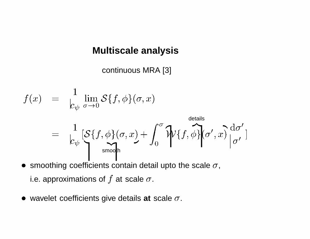
continuous MRA [3]
f(x) =
1c lim
�!0Sff; �g(�; x)
=
1c [Sff; �g(�; x)| {z }smooth
+Z �
0
detailsz }| {
Wff; �g(�0; x)d�0
�0]
� smoothing coefficients contain detail upto the scale �,
i.e. approximations of f at scale �.
� wavelet coefficients give details at scale �.
Holder regularity
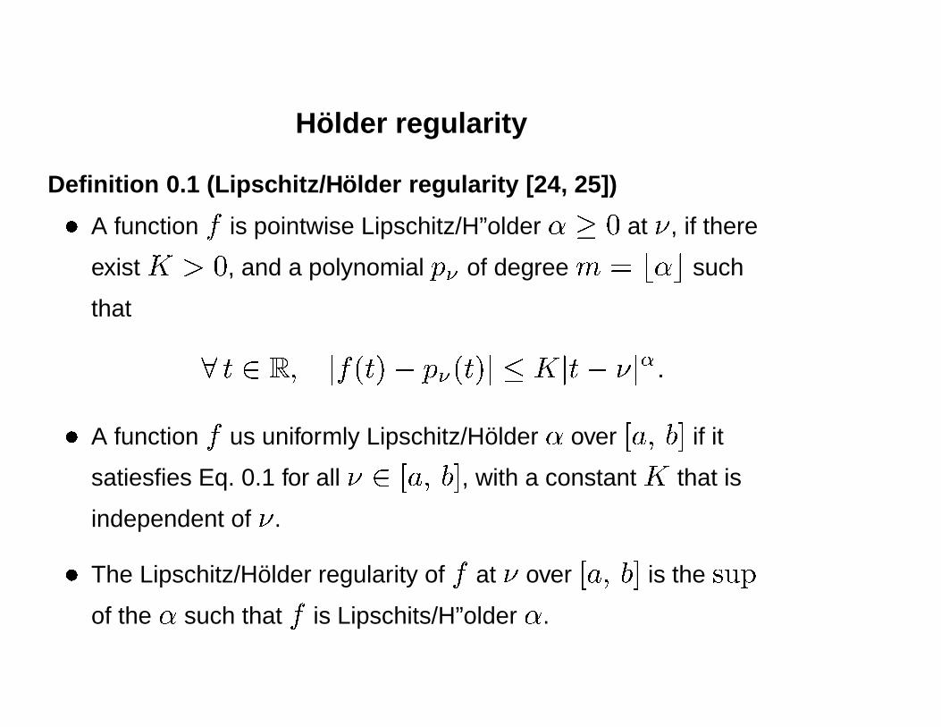
Definition 0.1 (Lipschitz/Holder regularity [24, 25])
� A function f is pointwise Lipschitz/H”older � � 0 at �, if there
exist K > 0, and a polynomial p� of degree m = b�c such
that
8 t 2 R ; jf(t)� p�(t)j � Kjt� �j�:
� A function f us uniformly Lipschitz/Holder � over [a; b] if it
satiesfies Eq. 0.1 for all � 2 [a; b], with a constant K that is
independent of �.
� The Lipschitz/Holder regularity of f at � over [a; b] is the sup
of the � such that f is Lipschits/H”older �.

Holder regularity
� Holder exponents measures the remainder of a Taylor
expansion, i.e.j"�(t)j = jf(t)� p�(t)j � Kjt� �j�:
� Characterize the local scaling properties.
� Measure the local regularity/differentiability.
� Is linked to the decay rate of the Fourier and wavelet
coefficients.
� Vanishing moment property of wavelets
Wff; g(�; t) =Wf"� ; g(�; t)
detrends the data!!!!

Simply speaking
Lipschitz/Holder exponents measure
jf(t+�t)� f(t)j � Kj�j�
for K finite.
Measures the local differentiability:
� � � 1, f(t) is continuous and differentiable.
� 0 < � < 1, f(t) is continuous but non-differentiable.
� �1 < � � 0, f(t) is discontinuous and non-differentiable.
� � � �1, f(t) is not longer locally integrable ) tempered
distribution, e.g. Delta Dirac for � = �1.

Multiscale analysis
WTMML’S
Continuous wavelet transform is redundant.
Definea a connected curve of local modulus maxima, i.e. points
where jWff; g(�; x)j is locally maximum at x = x0,
@xWff; g(�; x0) = 0:
This curve is called a modulus maxima line, a WTMML.
Analyze behavior of wavelet coefficients along the WTMML’s and
within the cone of influence, i.e. for the ith WTMML analyze
Wff; g(�; x) for x 2 fXi(�)g ^ jx� xij � C�
a1 per cone of influence

More precisely
Definition 0.2 (Wavelet transform modulus maxima [24, 25])
Let Wff; g(�; x) be the wavelet transform of a function f(x).
� A local extremum is any point (�0; x0) for which
@xWff; g(�; x) has a zero-crossing at x = x0, when x
varies.
� Call a wavelet transform modulus maximum, a WTMM, any point
(�0; x0) such that jWff; g(�0; x)j < jWff; g(�0; x0)j
when x belongs to either the right or the left neighbourhood of
x0, and jWff; g(�0; x)j � jWff; g(�0; x0)j when x
belongs to the other side of the neighbourhood of x0.
� Call a wavelet transform modulus maxima line, a WTMML, any

connected curve in the scale space (�; x) along which all
points are modulus maxima.

Multiscale analysis
local analysis
For a wavelet with a support [�C;C] one finds for the ith
WTMML [24, 25]
jWff; g(�; x)j � A�� for x 2 fXi(�)g
and this gives information on the local Holder/Lipschitz regularitya of
the tempered distribution f . Equivalent to
log jWff; g(�; x)j � logA+ � log � for x 2 fXi(�)g:
aExcluding oscilatory singularities.
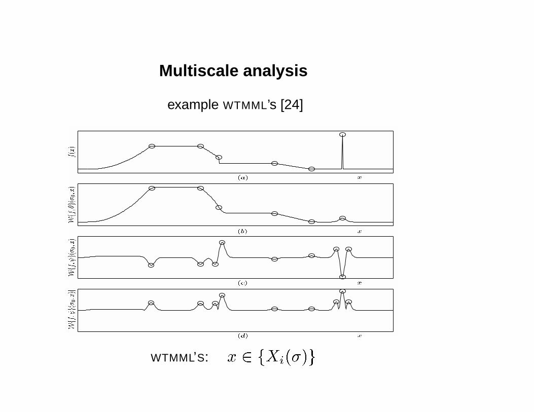
Multiscale analysis
example WTMML’s [24]
f(x)
(a) x
Wff;�g(� 0;x
)
(b) x
Wff; g(� 0;x
)
(c) x
jWff; g(� 0;x
)j
(d) xWTMML’S: x 2 fXi(�)g

Multiscale analysis
example WTMML’s [24]
−1 −0.8 −0.6 −0.4 −0.2 0 0.2 0.4 0.6 0.8 1
0
0.5
1
1.5
−1 −0.8 −0.6 −0.4 −0.2 0 0.2 0.4 0.6 0.8 1
1.5
2
2.5
3
3.5
4
1.5 2 2.5 3 3.5
3
4
5
6
7
8
2 3 4 2 3 4 2 3 4
f(x)
log�
log �
jlogW
TMMLj
log � log � log �
(a) x
(b) x
(c)
WTMML’S: x 2 fXi(�)g

Multiscale analysis
Algebraic singularities:��+(x) ,
8<:
0 x � 0
x�
�(�+1) x > 0;
and
���(x) ,8<
:�x�
�(�+ 1)
x � 0
0 x > 0;
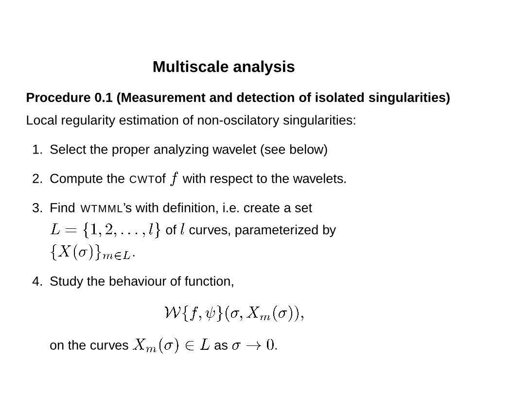
Multiscale analysis
Procedure 0.1 (Measurement and detection of isolated singularities)
Local regularity estimation of non-oscilatory singularities:
1. Select the proper analyzing wavelet (see below)
2. Compute the CWTof f with respect to the wavelets.
3. Find WTMML’s with definition, i.e. create a set
L = f1; 2; : : : ; lg of l curves, parameterized by
fX(�)gm2L.
4. Study the behaviour of function,
Wff; g(�;Xm(�));
on the curves Xm(�) 2 L as � ! 0.

5. Use the linear relationship to fit slope.

Multiscale analysis
1 2 3 4 5 6
0
2
4
6
8
10
12
1 2 3 4 5 6
0
2
4
6
8
10
12
−1 −0.8 −0.6 −0.4 −0.2 0 0.2 0.4 0.6 0.8 1
1
1.5
2
2.5
3
3.5
4
4.5
5
5.5
6
−1 −0.8 −0.6 −0.4 −0.2 0 0.2 0.4 0.6 0.8 1
1
1.5
2
2.5
3
3.5
4
4.5
5
5.5
6
−1 −0.8 −0.6 −0.4 −0.2 0 0.2 0.4 0.6 0.8 1
0
0.2
0.4
0.6
0.8
1
−1 −0.8 −0.6 −0.4 −0.2 0 0.2 0.4 0.6 0.8 1
0
0.2
0.4
0.6
0.8
1
(c)
jlog
WT
MM
L j
log �
v.m. : 2
reg. : 1
��est : �1
(f)
jlog
WT
MM
L j
log �v.m. : 2
reg. : 1
��est : 0:02
(b)
log�
x (e)
log�
x
(a)
f(x
)
x (d)
f(x
)
x

Multiscale analysis
1 2 3 4 5 6
0
2
4
6
8
10
12
1 2 3 4 5 6
0
2
4
6
8
10
12
−1 −0.8 −0.6 −0.4 −0.2 0 0.2 0.4 0.6 0.8 1
1
1.5
2
2.5
3
3.5
4
4.5
5
5.5
6
−1 −0.8 −0.6 −0.4 −0.2 0 0.2 0.4 0.6 0.8 1
1
1.5
2
2.5
3
3.5
4
4.5
5
5.5
6
−1 −0.8 −0.6 −0.4 −0.2 0 0.2 0.4 0.6 0.8 1
0
0.2
0.4
0.6
0.8
1
−1 −0.8 −0.6 −0.4 −0.2 0 0.2 0.4 0.6 0.8 1
0
0.2
0.4
0.6
0.8
1
(c)
jlog
WT
MM
L j
log �
v.m. : 2
reg. : 1
��est : 0:47
(f)
jlog
WT
MM
L j
log �v.m. : 2
reg. : 1
��est : �0:52
(b)
log�
x (e)
log�
x
(a)
f(x
)
x (d)
f(x
)
x

Multiscale analysis
1 2 3 4 5 6 7 815
17.5
20
22.5
25
1 2 3 4 5 6 7 815
17.5
20
22.5
25
1 2 3 4 5 6 7 815
17.5
20
22.5
25
1 2 3 4 5 6 7 815
17.5
20
22.5
25
0 240 480 720 960 1200 1440 1680 1920 2160 2400
1
2
3
4
5
6
7
8
0 240 480 720 960 1200 1440 1680 1920 2160 24001000
2000
3000
4000
5000
� = 0:2063
(c)
log(
WTM
ML )
log �
� = �0:8344
(d)
log(
WTM
ML )
log �
� = �0:006437
(e)
log(
WTM
ML )
log �
� = 0:5208
(f)
log(
WTM
ML)
log �
(b)
log�
x3[m]
(a)
c p
x3[m]
Estimation � using ln jWff; gg(ln�; x)j � lnC + � ln�

Scaling regimes
1 2 3 4 5 6 7 82
3
4
5
6
−1 −0.8 −0.6 −0.4 −0.2 0 0.2 0.4 0.6 0.8 1
1
2
3
4
5
6
7
8
−1 −0.8 −0.6 −0.4 −0.2 0 0.2 0.4 0.6 0.8 1
0
5
10
x 10−3
(c)
jlo g
WT
MM
L j
log �
Vanishing moments: 2
Smoothness wavelet: 1
Singularity �small : 0:01668
Singularity �large : �0:963
(b)
log�
x
(a)
f(x
)
x

Scaling regimes
1 2 3 4 5 6 7 8−2
0
2
4
6
−1 −0.8 −0.6 −0.4 −0.2 0 0.2 0.4 0.6 0.8 1
1
2
3
4
5
6
7
8
−1 −0.8 −0.6 −0.4 −0.2 0 0.2 0.4 0.6 0.8 1
0
5
10
15
x 10−3
(c)
jlo g
WTM
ML j
log �
Vanishing moments: 2
Smoothness wavelet: 1
Singularity �small : 1:927Singularity �large : �0:9658
(b)
log�
x
(a)
f(x
)
x

Scaling regimes
Box car:�(�) =
8<:
0 as � ! �0
�1 as � ! +1:
Gaussian bellshape:
�(�) =8<
:M as � ! �0
�1 as � ! +1:
Formally regularity statements can only be made as � ! 0.
Practically: Statements on regularity depend on the scale you
look at!! (see also discussions in [11, 13, 25])

Observations
� WTMML’s point to the singularities.
� Local scaling exponent varies, i.e.
jf(t+�t)� f(t)j � Kj�j�(t)
for K finite and � varying .... randomly
� The densification of the singularities makes it difficult to
estimate the local regularity ) interferring singularities
(bifurcations of WTMML’s).

Wavelet properties
0 0.5 1 1.5 2 2.5 3 3.5 4 4.5−1
0123456
−1 −0.8 −0.6 −0.4 −0.2 0 0.2 0.4 0.6 0.8 1
0
0.5
1
1.5
2
2.5
3
3.5
4
4.5
−1 −0.8 −0.6 −0.4 −0.2 0 0.2 0.4 0.6 0.8 1−1
−0.5
0
0.5
1
(c)
jlog
WTM
ML j
log �
Vanishing moments: 0
Smoothness wavelet: 1
Singularity �mean : �1:985
(b)
log�
x
(a)
f(x
)
x

Wavelet properties
0 0.5 1 1.5 2 2.5 3 3.5 4 4.5−1
0123456
−1 −0.8 −0.6 −0.4 −0.2 0 0.2 0.4 0.6 0.8 1
0
0.5
1
1.5
2
2.5
3
3.5
4
4.5
−1 −0.8 −0.6 −0.4 −0.2 0 0.2 0.4 0.6 0.8 1−1
−0.5
0
0.5
1
(c)
jlog
WTM
ML j
log �
Vanishing moments: 0
Smoothness wavelet: 0
Singularity �mean : �1
(b)
log�
x
(a)
f(x
)
x

Global multiscale analysis
(Multi-)fractals are examples of constructs with infinitely many
singularities.
Typically generated by some iterative non-linear operation.
Examples are the Cantor set, fractional Brownian motions and
binomial multifractals.
Characterized by fractal dimensions.

Fractal dimensions
Definition 0.3 (Fractal box-dimension or capacity [23, 27, 28])
The box dimension of a set A � Rp is given by,
DB , lim�#0
logN�
log ��1;
where N� is the minimum number of p-dimensional �-sized
neighbourhoods needed to cover the set A. The parameter � refers
to the size of the boxes, the length of their “gauge”.
DB = limj!1
log 2j
log 3j=log 2
log 3= 0:6309 � � � :

Fractal dimensions
0 0.1 0.2 0.3 0.4 0.5 0.6 0.7 0.8 0.9 10
0.5
1
1.5
2
Z x0
d�(x)

Fractal dimensions
Definition 0.4 (Hausdorff dimension and Hausdorff measure [9, 27, 28])
Consider a covering of the subset A � Rp by p-dimensional
neighbourhoods of linear size �i. The Hausdorff dimension dimH
is the critical dimension for which the Hausdorff measure Hd(�)
takes a finite value,
Hd(�) , lim�#0infX
i
�di =8>><
>>:0 d > dimH ;
finite d = dimH ;
1 d < dimH ;
and where the infimum extends over all possible coverings subject
to the constraint that �i � �.

Fractal dimensions
Definition 0.5 (Generalized or Renyi dimensions Dq [34, 27, 10, 32])
To define the generalized dimensionsDq partition the measure
using a grid with a lattice constant � and subsequently introduce the
multiscale partition function as
Z�(q) ,
X8xi2A�[B�(xi)]q =
X8xi2Apiq;
where pi = �[B�(xi)] ,R
B�(xi)d�(x) is the total measure
within the ith box, at position xi and of linear size �. The set of
generalized dimensions Dq is then defined by,
(q � 1)Dq , �(q) , lim�#0
logZ�(q)
log �
;

implying a scaling behaviour for the partition function Z�(q), for
small �,Z�(q) / ��(q)
and where �(q) is the mass exponent function.

Fractal dimensions
For the binomial multifractal the partition function for the kth
iteration equals
Z�=2�k(q) = (pq1 + pq2)k = �(q)k;
with �(q) the generator, i.e. the partition function after the first
iteration.
Generalized dimensions Dq :
(q � 1)Dq = � log2 �(q) = � log2(pq
1 + pq2);
which are – by nature of the self-similar construction – fully
determined by the generator.

Fractal dimensions
−1 −0.8 −0.6 −0.4 −0.2 0 0.2 0.4 0.6 0.8 10
0.5
1
1.5
2
2.5
3
−1 −0.8 −0.6 −0.4 −0.2 0 0.2 0.4 0.6 0.8 10123
−1 −0.8 −0.6 −0.4 −0.2 0 0.2 0.4 0.6 0.8 10123
−1 −0.8 −0.6 −0.4 −0.2 0 0.2 0.4 0.6 0.8 10
1
2
binomial multifractal

Fractal dimensions
Definition 0.6 (Local scaling exponent of a measure [6, 36, 1, 18])
The local scaling exponent or local fractal dimension of a measure
� is defined as
�(x0) , lim�#0inflog �(B�(x0))
log �
where B�(x0) is a �-box centered at x0.
� Notice the similarity with the definition of local Holder regularity.
� Original multifractal framework build on measure theoretical
arguments.

Fractal dimensions
Theorem 0.1 (Singularity spectrum and generalized dimensions [6, 18])
The singularity spectrum and the generalized fractal dimensions are
related via a Legendre transforms8<:
�(q) = q�� f(�)
q = @�f(�)and conversely, 8<
:f(�) = q�� �(q)
� = @q�(q):

Fractal dimensions
Hausdorff dimensions f(�) can be associated with the subsets
A� � A according tof(�) , lim
�#0�logN�(�)
log �
which is equivalent to the following scaling behaviour
N�(�) / ��f(�)���
�#0:
By summing over A�:
Z�(q) =X
�
Xx2A�
�[B�(x)]q /Z
�q��f(�)d�;

Fractal dimensions
Definition 0.7 (Singularity spectrum of a measure [6, 32, 1, 18])
The singularity spectrum of a measure �(x) is the function f(�)
such that
f(�) , dimHfx j �[B�(x)] / ��j�#0g;
where dimH denotes the Hausdorff dimension and B�(x) is a
�-box centered at x.

Fractal dimensions
For binomial multifractal:
�(q) = � log2[pq
1 + pq2]; Dq =
�(q)
q � 1
and the singularity spectrum reads
f(�) = �c(�) log2 c(�)� (1� c(�)) log2(1� c(�));
with c(�) = (�� �min)=(�max � �min) and
�min = � log2 p1; �max = � log2 p2.

Fractal dimensions
−20 0 200
0.5
1
1.5
2
−20 0 20−60
−40
−20
0
20
0 1 20
0.5
1
q
Dq
q
�(q)
�
f(�)

Fractal dimensions
So far analysis limited to measures.
Extension to multifractal functions:
f(x) ,Z x
0
d�(x0) + Pn(x);
where �(x) 2M and Pn(x) a polynomial of arbitrary but finite
order n.

Multiscale analysis
Theorem 0.2 (Generalized fractal dimensions of a function by the WTMML [1])
Let � 2 M. Let Pn(x) be a polynomial of the order n and
f(x) =R x
0
d�(x0) + Pn(x). Let be an analyzing wavelet with
M > n vanishing moments, i.e. 8k; 0 � k � n;R
xk (x)dx = 0.
Let Z�f�; g(p; q) be the corresponding partition function
Z�ff; g(p; q) = j�j�pX
j2J( sup
x=Xj(�)jhf; �;xij)q; q 2 R ;
where fXj(�)gj2J is the set of WTMML’s. Then, for all q 2 R , �(q) is
the transition exponent such that
p < �(q) ) lim�#0Z�ff; g(p; q) = 0
p > �(q) ) lim�#0Z�ff; g(p; q) =1:

Singularity spectrum
Definition 0.8 (Singularity spectrum of a function Bacry93,Holschneider95)
A singularity spectrum of a function f(x) is the function f(�),
� 2 Hf , the set of finite Holder exponents of f , such that
f(�) = dimHfx0 2 R j�(x0) = �g;
where dimH denotes the Hausdorff dimension.

Isolated singularities
0 2 4 6−60
−25
10
45
80
−5 −2.5 0 2.5 5−3
−1.5
0
1.5
3
−1 −0.5 0 0.5 1−1
−0.5
0
0.5
1
−1 −0.8 −0.6 −0.4 −0.2 0 0.2 0.4 0.6 0.8 1
0
2
4
6
−1 −0.8 −0.6 −0.4 −0.2 0 0.2 0.4 0.6 0.8 10
10
20
30
40
(c)
Z(�;q)
(d)
�(q)
(e)
f(�)
(b)
log�
(a)
f(x
)
log � q �x
x
0 2 4 6−40
−20
0
20
40
−5 −2.5 0 2.5 5−3
−1.5
0
1.5
3
−1 −0.5 0 0.5 1−1
−0.5
0
0.5
1
−1 −0.8 −0.6 −0.4 −0.2 0 0.2 0.4 0.6 0.8 1
0
2
4
6
−1 −0.8 −0.6 −0.4 −0.2 0 0.2 0.4 0.6 0.8 10
0.5
1
1.5
(c)
Z(�;q)
(d)
�(q)
(e)
f(�)
(b)
log�
(a)
f( x
)
log � q �x
x
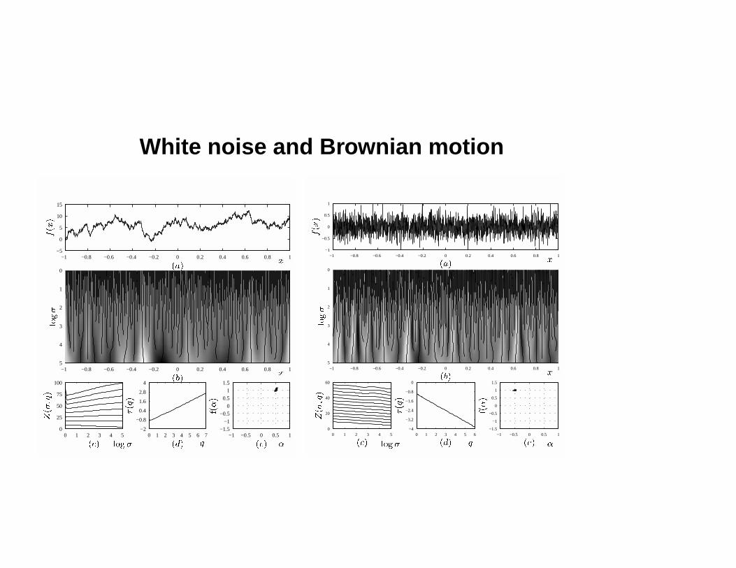
White noise and Brownian motion
0 1 2 3 4 50
25
50
75
100
0 1 2 3 4 5 6 7−2
−0.8
0.4
1.6
2.8
4
−1 −0.5 0 0.5 1−1.5
−1
−0.5
0
0.5
1
1.5
−1 −0.8 −0.6 −0.4 −0.2 0 0.2 0.4 0.6 0.8 1
0
1
2
3
4
5
−1 −0.8 −0.6 −0.4 −0.2 0 0.2 0.4 0.6 0.8 1−5
0
5
10
15
(c)
Z(�;q)
(d)
�(q)
(e)
f(�)
(b)
log�
(a)
f(x
)
log � q �x
x
0 1 2 3 4 50
20
40
60
0 1 2 3 4 5 6−4
−3.2
−2.4
−1.6
−0.8
0
−1 −0.5 0 0.5 1−1.5
−1
−0.5
0
0.5
1
1.5
−1 −0.8 −0.6 −0.4 −0.2 0 0.2 0.4 0.6 0.8 1
0
1
2
3
4
5
−1 −0.8 −0.6 −0.4 −0.2 0 0.2 0.4 0.6 0.8 1−1
−0.5
0
0.5
1
(c)
Z( �;q)
(d)
�( q)
(e)
f(�)
(b)
log�
(a)
f(x
)
log � q �x
x

fractional Brownian motions
Partition function:
Z�(q) / ��1
2
q�1;displays a trivial (in q) scaling behavior =) monofractal.

Binomial multifractal
1 2 3 4 50
10
20
30
40
−5 −3 −1 1 3 5−10
−6
−2
2
6
10
−2 −1 0 1 2 3 40
0.5
1
−1 −0.8 −0.6 −0.4 −0.2 0 0.2 0.4 0.6 0.8 1
1
2
3
4
5
−1 −0.8 −0.6 −0.4 −0.2 0 0.2 0.4 0.6 0.8 10
0.5
1
(c)
Z(�;q)
(d)
�(q)
(e)
f(�)
(b)
log�
(a)
f(x
)
log � q �x
x
1 2 3 4 55
8
11
14
17
20
−5 −3 −1 1 3 5−10
−6
−2
2
6
10
−2 −1 0 1 2 3 40
0.5
1
−1 −0.8 −0.6 −0.4 −0.2 0 0.2 0.4 0.6 0.8 1
1
1.8
2.6
3.4
4.2
5
−1 −0.8 −0.6 −0.4 −0.2 0 0.2 0.4 0.6 0.8 10
0.02
0.04
0.06
(c)
Z( �;q)
(d)
�(q)
(e)
f(�)
(b)
log�
(a)
df( x)
dx
log � q �x
x

Important exponents
� conservation of the mean (index fbm)
H , f�(q)gq=1 + 1;
� endpoints f(�)�min =max , f@q�(q)gq!�1:
� information dimension
�1 , f@q�(q)gq=1 with D1 = f(�1)
� dimension singular support
�0 , f@q�(q)gq=0 with D0 = f(�0)

Multiscale analysis
1 2 3 4 5 6 7 8−200
−100
0
100
200
300
−9 −4.4 0.2 4.8 9.4 14−20
−16
−12
−8
−4
0
−1 −0.4 0.2 0.8 1.4 2−0.5
0
0.5
1
1.5
0 240 480 720 960 1200 1440 1680 1920 2160 2400
1
2
3
4
5
6
7
8
0 240 480 720 960 1200 1440 1680 1920 2160 24001000
2000
3000
4000
5000(c)
logZ
(�;q
)
(d)
�(q)
(e)
f( �)
(b)
log�
(a)
c p
log � q �x[m]
x[m]
Estim. �(q), f(�) using ln jZ(ln�; q)j � lnC + �(q) ln�.
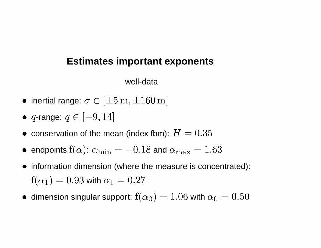
Estimates important exponents
well-data
� inertial range: � 2 [�5m;�160m]
� q-range: q 2 [�9; 14]
� conservation of the mean (index fbm): H = 0:35
� endpoints f(�): �min = �0:18 and �max = 1:63
� information dimension (where the measure is concentrated):
f(�1) = 0:93 with �1 = 0:27
� dimension singular support: f(�0) = 1:06 with �0 = 0:50

Multiscale analysis
Global analysis cp well data
2 4 6
−100
0
100
200
300
−5 0 5 10−10
−5
0
0 0.5 10
0.5
1
−1 −0.8 −0.6 −0.4 −0.2 0 0.2 0.4 0.6 0.8 1
1
2.2
3.4
4.6
5.8
7
−1 −0.8 −0.6 −0.4 −0.2 0 0.2 0.4 0.6 0.8 1
(c)
logZ(�;q
)
(d)
�(q)
(e)
f(�)
(b)
log�
(a)
r(t)

Multiscale analysis
Global analysis cs well data
2 4 6
−100
0
100
200
300
−5 0 5 10−10
−5
0
0 0.5 10
0.5
1
−1 −0.8 −0.6 −0.4 −0.2 0 0.2 0.4 0.6 0.8 1
1
2.2
3.4
4.6
5.8
7
−1 −0.8 −0.6 −0.4 −0.2 0 0.2 0.4 0.6 0.8 1
(c)
Z(�;q)
(d)
�(q)
(e)
f(�)
(b)
log�
(a)
r(t)

Multiscale analysis
Global analysis � well data
2 4 6
−100
0
100
200
300
−5 0 5 10−15
−10
−5
0
0 0.5 1 1.50
0.5
1
−1 −0.8 −0.6 −0.4 −0.2 0 0.2 0.4 0.6 0.8 1
1
2.2
3.4
4.6
5.8
7
−1 −0.8 −0.6 −0.4 −0.2 0 0.2 0.4 0.6 0.8 1
(c)
Z(�;q)
(d)
�(q)
(e)
f(�)
(b)
log�
(a)
r(t)
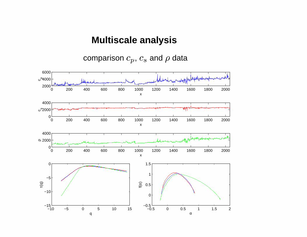
Multiscale analysis
comparison cp, cs and � data
0 200 400 600 800 1000 1200 1400 1600 1800 20002000
4000
6000
x
c p
0 200 400 600 800 1000 1200 1400 1600 1800 20000
2000
4000
x
c s
0 200 400 600 800 1000 1200 1400 1600 1800 20000
2000
4000
x
ρ
−10 −5 0 5 10 15−15
−10
−5
0
q
τ(q)
−0.5 0 0.5 1 1.5 2−0.5
0
0.5
1
1.5
α
f(α)

Multiscale analysis
comparison different wells
0 500 1000 1500 2000 2500 3000 3500 40000
5000
x
c p
Well A
0 200 400 600 800 1000 1200 1400 1600 1800 20002000
4000
6000
x
c p
Well B
−10 −5 0 5 10 15−15
−10
−5
0
q
τ(q)
−0.5 0 0.5 1 1.5 2−0.2
0
0.2
0.4
0.6
0.8
1
1.2
1.4
α
f(α)

Multiscale analysis
Global analysis reflection coefficients
2 4 6
0
100
200
−5 0 5 10−20
−10
0
10
−1 −0.5 0
0
0.5
1
−1 −0.8 −0.6 −0.4 −0.2 0 0.2 0.4 0.6 0.8 1
1
2.2
3.4
4.6
5.8
7
−1 −0.8 −0.6 −0.4 −0.2 0 0.2 0.4 0.6 0.8 1
(c)
Z(�;q)
(d)
�(q)
(e)
f(�)
(b)
log�
(a)
r(t)

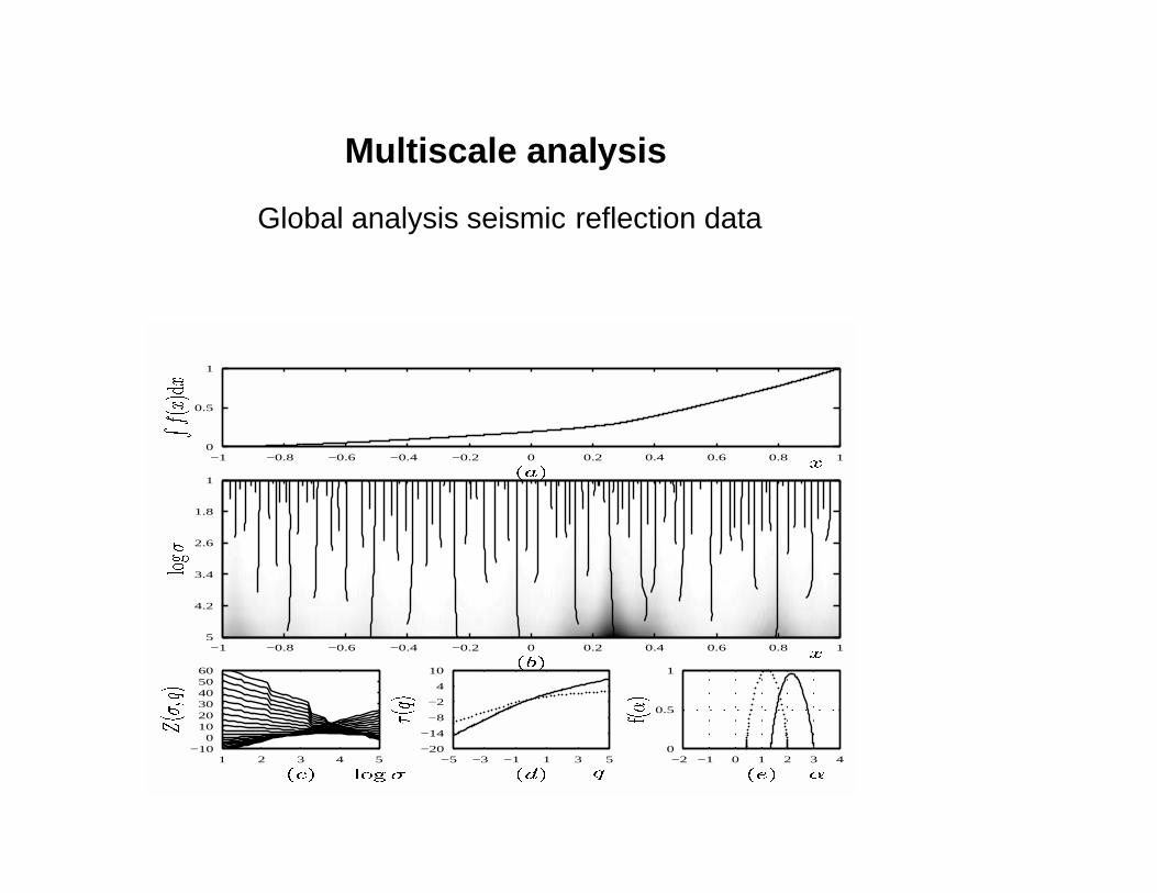
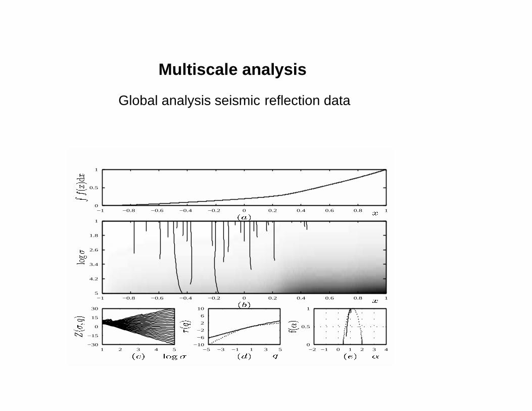
Multiscale analysis
Global analysis seismic reflection data
1 2 3 4
−50
0
50
100
150
−4 0.5 5−20
−16
−12
−8
−4
0
−2.5 −1.625−0.75 0.125 1−0.5
−0.25
0
0.25
0.5
0.75
1
−1 −0.8 −0.6 −0.4 −0.2 0 0.2 0.4 0.6 0.8 1
1
1.7
2.4
3.1
3.8
4.5
−1 −0.8 −0.6 −0.4 −0.2 0 0.2 0.4 0.6 0.8 1
O6 O6 O6
O6
O6
(c)
Z(�;q
)
(d)
�(q )
(e)
f(�)
(b)
log�
(a)
r(t)

Estimates important exponents
reflection-data
� inertial range: � 2 [0:008 s; 0:09 s]
� q-range: q 2 [�4; 5]
� endpoints f(�): �min = �2:22 and �max = 0:43
� information dimension (where the measure is concentrated):
f(�1) = 0:80 with �1 = 1:76
� dimension singular support: f(�0) = 0:98 with �0 = 1:35

Properties
� Differentiation shifts the singularity spectrum to the left, i.e.@�f : f(�) := f(�+ �)
� Integration shifts the singularity spectrum to the right, i.e.
I�f = @��f : f(�) := f(�� �)
� Observation range singularities (� 2 (�min; �max)) depends
on smoothness and number of vanishing moments.

Wavelet properties
−1 0 1−2
−1
0
1
2
−2 −1 0 1 2−2
−1
0
1
2
−1 0 1−2
−1
0
1
2
−2 −1 0 1 2−2
−1
0
1
2
−1 0 1−2
−1
0
1
2
−2 −1 0 1 2−2
−1
0
1
2
−1 0 1−2
−1
0
1
2
−2 −1 0 1 2−2
−1
0
1
2
Gaussian f(�) Derivative Gaussian f(�)
Boxcar f(�) Poor Man f(�)
Multiscale analysis
Global analysis seismic reflection data
1 2 3 4 5−10
0102030405060
−5 −3 −1 1 3 5−20
−14
−8
−2
4
10
−2 −1 0 1 2 3 40
0.5
1
−1 −0.8 −0.6 −0.4 −0.2 0 0.2 0.4 0.6 0.8 1
1
1.8
2.6
3.4
4.2
5
−1 −0.8 −0.6 −0.4 −0.2 0 0.2 0.4 0.6 0.8 10
0.5
1
(c)
Z(�;q
)
(d)
� (q)
(e)
f(�)
(b)
log�
(a)
R f(x)
d x
log � q �x
x
Multiscale analysis
Global analysis seismic reflection data
1 2 3 4 5−30
−15
0
15
30
−5 −3 −1 1 3 5−10
−6
−2
2
6
10
−2 −1 0 1 2 3 40
0.5
1
−1 −0.8 −0.6 −0.4 −0.2 0 0.2 0.4 0.6 0.8 1
1
1.8
2.6
3.4
4.2
5
−1 −0.8 −0.6 −0.4 −0.2 0 0.2 0.4 0.6 0.8 10
0.5
1
(c)
Z(�;q
)
(d)
� (q)
(e)
f(�)
(b)
log�
(a)
R f(x)
d x
log � q �x
x

Multiscale analyis
Besov Norms [20, 33]
A function f belongs to the homogeneous Besov space Bs;qp if
Z +1
0
[1
�skWff; g(�; �)kLp ]q d�
�
<1
with s 2 R and p; q > 0. Hence
�(p) = supfs : F 2 Bs=p;pp g = supfs : f 2 Lp;s=pg
with f 2 Ls;p () f 2 Lp ^ @sxf 2 Lp.

Multiscale analysis
Besov norm, measurability, differentiability ....
� Besov norm is finite if sp < �(p) + 1 iff s < M with M# van.
mom. and regularity wavelet [35].
� When �1 = limp!1 @p�(p) < 0 f is not bounded!
� Besov norm is related to the global (ir)-regularity.
� Singularities ly dense, i.e. f(�) is smooth, there is no phase
transition.
Of course this is all “true” if one assumes that the discete data
constitute samples from a “continuous” function/functional!

Multiscale analyis
Besov Brownian motion, white noise
0 5 10−0.5
0
0.5
1
1.5
2
2.5
3
p
τ(p)
0 5 100.5
0.51
0.52
0.53
p
τ(p)
/p+
1/p
Brownian Motion
0.45 0.5 0.55 0.60.9
0.95
1
1.05
1.1
1.15
1.2
α
f(α)
0 2 4 6−4
−3.5
−3
−2.5
−2
−1.5
−1
p
τ(p)
0 2 4 6−0.48
−0.478
−0.476
−0.474
−0.472
−0.47
−0.468
p
τ(p)
/p+
1/p
White Noise
−0.5 −0.48 −0.46
0.98
1
1.02
1.04
α
f(α)

Multiscale analyis
Besov Devil Staircase
0 2 4 6−0.5
0
0.5
1
1.5
2
p
τ(p)
0 2 4 60.5
0.6
0.7
0.8
0.9
1
p
τ(p)
/p+
1/p
Devil staircase
0.2 0.4 0.6 0.8−0.2
0
0.2
0.4
0.6
0.8
α
f(α)
0 2 4 6−3.5
−3
−2.5
−2
−1.5
−1
−0.5
p
τ(p)
0 2 4 6−0.5
−0.4
−0.3
−0.2
−0.1
0
0.1
p
τ(p)
/p+
1/p
Devil Staircase distribution
−0.8 −0.6 −0.4 −0.2−0.2
0
0.2
0.4
0.6
0.8
α
f(α)

Multiscale analyis
Besov Well
0 5 10 15−3
−2.5
−2
−1.5
−1
−0.5
p
τ(p)
0 5 10 15−0.15
−0.1
−0.05
0
0.05
0.1
0.15
0.2
p
τ(p)
/p+
1/p
Well−log
−0.2 0 0.20
0.2
0.4
0.6
0.8
1
α
f(α)
0 5 10 15−20
−15
−10
−5
0
p
τ(p)
0 5 10 15−1.3
−1.2
−1.1
−1
−0.9
−0.8
p
τ(p)
/p+
1/p
Reflection
−1.5 −1 −0.5−0.2
0
0.2
0.4
0.6
0.8
1
α
f(α)

Multiscale analyis
Besov Seismic
0 5 10 15−2.5
−2
−1.5
−1
−0.5
p
τ(p)
0 5 10 15−0.2
−0.1
0
0.1
0.2
0.3
0.4
p
τ(p)
/p+
1/p
Well−log
−0.2 0 0.2 0.4−0.2
0
0.2
0.4
0.6
0.8
1
α
f(α)
0 2 4 6−12
−10
−8
−6
−4
−2
p
τ(p)
0 2 4 6−2
−1.9
−1.8
−1.7
−1.6
−1.5
p
τ(p)
/p+
1/p
Reflection
−2.5 −2 −1.5−0.4
−0.2
0
0.2
0.4
0.6
0.8
α
f(α)

Besov
� Regularity information can be used for linear inverse problems
(See Jonathan Kane’s SEG abstract and [4, 5, 31, 2])
� We know in what functional space the medium lies.
� We know in what functional space the reflection data lies.
� Multifractality means heterogeneous scaling:
jf(t+�t)� f(t)j � Kj�j�(t)

Observations
from the data
Both well and seismic data display multifractal behavior
� Well-data is, except for a sparse set of singularities, close to
continuous but not differentiable.
� Reflection data (both reflection coefficients and reflectivity)
are almost everywhere discontinuous and everywhere
non-differentiable.

Implications
There exists an unique solution for@xp(x; t) + �(x)@tv(x; t) = 0
@xv(x; t) + �(x)@tp(x; t) = 0
Iff
0 < �0 � �(x) � �1 <1
0 < �0 � �(x) � �1 <1
Is that true given the multiscale analysis findings?
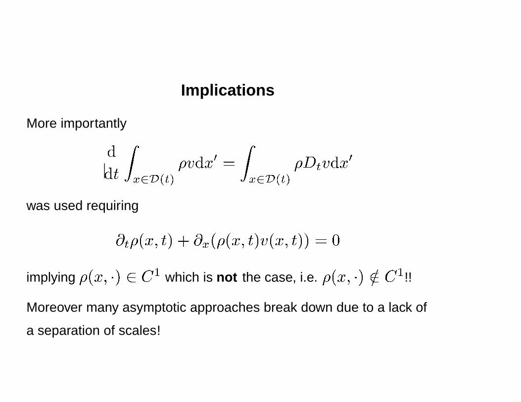
Implications
More importantly
ddt
Zx2D(t)�vdx0 =
Zx2D(t)�Dtvdx0
was used requiring
@t�(x; t) + @x(�(x; t)v(x; t)) = 0
implying �(x; �) 2 C1 which is not the case, i.e. �(x; �) =2 C1!!
Moreover many asymptotic approaches break down due to a lack of
a separation of scales!

Conclusions
well-data and seismic data
� Well and reflection data display a multifractal, heterogeneous
scaling behavior.
� Well-log are apparent non-smooth and even discontinuous.
� Singularity structure more or less shared by different physical
parameters.
� Singularity structure different wells is comparable.
� Reflection data are almost everywhere discontinuous and
certainly non-differentiable.
� Singularity spectra provide a priori information.
References[1] E. Bacry, J. F. Muzy, and A. Arneodo. Singularity spectrum of fractal signals from
wavelet analysis: Exact results. Journal of Statistical Physics, 70(3/4):635–674, 1993.
[2] K. Berkner, M. Gormish, and E. Schwartz. Multiscale sharpening and smoothing
in besov spaces with applications to image enhancement. Appl. Comput. Harmon.
Anal., 2001. to appear March/June 2001.
[3] R. Carmona, W. Hwang, and B. Torresani. Practical time-frequency analysis. Aca-
demic Press, 1998.
[4] H. Choi and R. G. Baraniuk. Wavelet statistical models and besov spaces. In Pro-
ceedings of SPIE Technical Conference on Wavelet Applications in Signal Processing
VII, 1999.
[5] H. Choi and R. G. Baraniuk. Information-theoretic analysis of besov spaces. In Pro-
ceedings of SPIE Technical Conference on Wavelet Applications in Signal and Image
Processing VIII, 2000.
[6] P. Collet. Dynamical Systems 1986, chapter Haussdorff dimension of the singularities
for invariant measures of expanding dynamical systems. Springer-Verlag, 1986.
[7] I. Daubechies. Ten lectures on wavelets. SIAM, Philadelphia, 1992.
81-1
[8] J. M. Ghez and S. Vaienti. Integrated wavelets on fractal sets: II. The generalized
dimensions. Nonlinearity, 5:791–804, 1992.
[9] F. Hausdorff. Dimension und außeres maß. Math. Analen, 79:157–179, 1918.
[10] H. G. E. Hentschel and I. Procaccia. The infinite number of generalized dimensions
of fractals on strange attractors. Physica D, 8:435–444, 1983.
[11] F. Herrmann. A scaling medium representation, a discussion on well-logs, fractals
and waves. PhD thesis, Delft University of Technology, Delft, the Netherlands, 1997.
http://wwwak.tn.tudelft.nl/�felix.
[12] F. Herrmann. Evidence of scaling for acoustic waves in multiscale media and its
possible implications. In Expanded Abstracts, Tulsa, 1998. Soc. Expl. Geophys.
[13] F. Herrmann. Multiscale analysis of well and seismic data. In S. Hassanzadeh, edi-
tor, Mathematical Methods in Geophysical Imaging V, volume 3453, pages 180–208.
SPIE, 1998.
[14] F. Herrmann. Singularity Characterization by Monoscale Analysis: Application to Seis-
mic Imaging. Appl. Comput. Harmon. Anal., 2001. to appear March/June 2001.
[15] F. Herrmann and C. Stark. Monoscale analysis of edges/reflectors using fractional
differentiations/integrations. In Expanded Abstracts, Tulsa, 1999. Soc. Expl. Geophys.
http://www-erl.mit.edu/�felix/Preprint/SEG99.ps.gz.
81-2

[16] F. Herrmann and C. Stark. A scale attribute for texture in well- and
seismic data. In Expanded Abstracts, Tulsa, 2000. Soc. Expl. Geophys.
http://www-erl.mit.edu/�felix/Preprint/SEG00.ps.gz.
[17] M. Holschneider. On the wavelet transform of fractal objects. Journal of Statistical
Physics, 50(5/6):963–993, 1987.
[18] M. Holschneider. Wavelets an analysis tool. Oxford Science Publications, 1995.
[19] S. Jaffard. Exposants de Holder en points donnes et coefficients d’ondelettes. C. R.
Acad. Sci. Paris, 308:79–81, 1989.
[20] S. Jaffard. Multifractal formalism for functions part I: Results valid for all functions.
SIAM J. Mathematical Analysis, 28(4):944–970, July 1997.
[21] S. Jaffard. Multifractal formalism for functions part II: Self-similar functions. SIAM J.
Mathematical Analysis, 28(4):971–998, July 1997.
[22] S. Jaffard and Y. Meyer. Wavelet Methods for Pointwise Regularity and Local Oscilla-
tions of Functions, volume 123. American Mathematical Society, september 1996.
[23] A. N. Kolmogorov. Local structure of turbulence in an incompressible liquid for very
large Reynolds numbers. Dokl. Akad. Nauk., 30:299–303, 1941.
[24] S. Mallat and L. Hwang. Singularity detection and processing with wavelets. IEEE
Transactions on Information Theory, 38(2):617–642, 1992.
81-3
[25] S. G. Mallat. A wavelet tour of signal processing. Academic Press, 1997.
[26] S. G. Mallat and S. Zhong. Characterization of signals from multiscale edges. IEEE
Trans. Patt. Anal. Mach. Intell., 14:710–732, 1992.
[27] B. B. Mandelbrot. Intermittent turbulence in self-similar cascades: divergence of high
moments and dimension of the carrier. J. Fluid Mechanics, 62:331, 1974.
[28] B. B. Mandelbrot. The fractal geometry of nature. Freeman and Co., 1982.
[29] J. Morlet, G. Arens, E. Fourgeau, and D. Giard. Wave propagation and sampling
theory-Part I: Complex signal and scattering in multilayerd media. Geophysics,
V(47):203–221, 1982.
[30] J. Morlet, G. Arens, E. Fourgeau, and D. Giard. Wave propagation and sampling
theory-Part II: Complex signal and scattering in multilayerd media. Geophysics,
V(47):222–236, 1982.
[31] R. Neelamani, H. Choi, and R. Baraniuk. Wavelet-based deconvolution for
ill-conditioned systems. IEEE Transactions on Image Processing. submitted,
www-dsp.rice.edu/�neelsh/publications.
[32] G. Parisi and U. Frisch. Turbulence and predictability in geophysical fluid dynamics
and climate dynamics, chapter A multifractal model of intermittency, pages 84–88.
North Holland, 1985.
81-4
[33] V. Perrier and C. Basdevant. Besov norms in terms of the continuous wavelet transfor-
m, application to structure functions. to appear in Mathematical Models and Methods
in the Applied Sciences (M3AS), 6(6), 1996.
[34] A. Renyi. Probability theory. North Holland, 1970.
[35] R. Riedi, M. Crouse, V. Ribeiro, and G. Baraniuk. A multifractal wavelet model with
application to network traffic. IEEE Transactions on Information Theory, 1998.
[36] A. P. Siebesma. Multifractals in condensed matter. PhD thesis, Rijksuniversiteit
Groningen, 1989.
81-5