Scale Up of Slurry Bubble Reactors

Oil & Gas Science and Technology – Rev. IFP, Vol. 61 (2006), No. 3, pp. 443-458Copyright © 2006, Institut français du pétrole

Scale Up of Slurry Bubble ReactorsA. Forret1, J.M. Schweitzer1, T. Gauthier1, R. Krishna2 and D. Schweich3

1 IFP-Lyon, BP 3, 69390 Vernaison - France2 Department of Chemical Engineering, University of Amsterdam, 1018 WV Amsterdam - The Netherlands

3 LGPC-CNRS, ESCPE, 43, boulevard du 11 Novembre, BP 2077, 69616 Villeurbanne - Francee-mail: [email protected] - [email protected] - [email protected] - [email protected] - [email protected]

Résumé — Extrapolation des réacteurs slurry — Les réacteurs à colonne à bulles trouvent de plus enplus d’applications dans l’industrie. Ils sont particulièrement appropriés pour mettre en œuvre desréactions très exothermiques, telles que la synthèse du méthanol ou la synthèse Fischer-Tropsch deconversion du gaz de synthèse en paraffines liquides. Les procédés industriels requièrent des réacteurs degros volumes, dont le diamètre peut atteindre 10 m, équipés d’échangeur de chaleur interne (tubesverticaux) afin de contrôler la température de réaction. La présente étude a pour objet la compréhensiondes effets de taille et de la présence des internes sur les caractéristiques hydrodynamiques pour contribuerà l’élaboration des règles d’extrapolation aux conditions industrielles des réacteurs slurry à partird’expériences menées en maquettes froides.

Notre étude montre que l’intensité de la recirculation liquide augmente fortement avec le diamètre de lacolonne alors que le taux de vide n’est que peu affecté. Deux méthodes sont proposées pour prédirel’effet de taille sur la vitesse liquide : une corrélation empirique tirée de la littérature ainsi qu’un modèlephénoménologique. Les tubes verticaux (simulant des échangeurs de chaleur) guident axialement lacirculation liquide, favorisant le transport convectif et diminuant les fluctuations de vitesse. Le mélangedu liquide est alors significativement affecté par la présence des internes. Il ne peut plus être décritcorrectement par le modèle standard mono dimensionnel de dispersion axial. Un modèle bidimensionnel,prenant en compte le profil radial de la vitesse liquide ainsi que la dispersion axiale et radiale est doncdéveloppé pour représenter le mélange du liquide dans une colonne à bulles avec internes.

Abstract — Scale Up of Slurry Bubble Reactors — Bubble column reactors are finding increasing use inindustrial practice. They are in particular appropriate to carry out highly exothermic reactions, such asmethanol synthesis or Fischer-Tropsch synthesis of conversion of synthesis gas to liquid paraffins.Industrial process require important volumes of reactors, the reactor diameter can reach 10 m. Tocontrol the reaction temperature, internal heat-exchange tubes (vertical tubes) are inserted inside thereactor. This study deals with the effects of scale and the presence of internals on hydrodynamiccharacteristics, for scale-up purposes based on experiments in cold mockups.

Our study shows that the liquid recirculation intensity depends strongly on the column diameter whereasthe gas holdup is slightly affected. Two methods are proposed to predict scale effect on liquid velocity: anempirical correlation proposed in the literature and a phenomenological model. Internals guide liquid:the large scale recirculation increases but fluctuations of liquid velocity decrease. Therefore the mixingof liquid is significantly affected by the presence of internals and is not well described by the standardmono dimensional axial dispersion model. A two-dimensional model, taking into account a radiallydependent axial velocity profile and both axial and radial dispersion, is therefore developed to describethe liquid mixing in a bubble column with internals.

http://ogst.ifp.fr/

http://www.ifp.fr/

NOTATIONS

ADM Axial Dispersion ModelC local tracer concentration (mol/m3)CL tracer concentration in liquid phase (mol/m3)C1 tracer concentration in the upflow liquid flow region

(mol/m3)C2 tracer concentration in the downflow liquid flow

region (mol/m3)C–

cross-sectional averaged tracer concentration(mol/m3)

CSTR Continuous Stirred Tank ReactorD column diameter (m)Dax liquid axial dispersion coefficient (m2/s)Dax,1D liquid axial dispersion coefficient determined by the

one-dimensional ADM (m2/s)Dax,2D liquid axial dispersion coefficient determined by the

two-dimensional model (m2/s)Drad,2D liquid radial dispersion coefficient determined by

the two-dimensional model (m2/s)dt diameter of vertical internals (m)H height of measurement or sampling (m)HD aerated height (m)N number of acquisition data pointsnt number of cooling tubesr radial coordinate (m)S column cross section area (π D2/4) (m2)

Sfree open cross section area or free surface (m2)

ui instantaneous liquid velocity (m/s)

r.m.s. fluctuation of the velocity

(m/s)Ug effective superficial gas velocity (Qg/Sfree) deter-

mined at pressure conditions prevailing just abovethe gas distributor (m/s)

time-averaged local axial liquid velocity (m/s)

VL(0) time-averaged center-line liquid velocity or maxi-mum upward velocity measured along column axis(m/s)

x dimensionless radial coordinate x = 2r/Dxinv dimensionless radial coordinate at the flow reversalz dimensionless axial coordinate z = H/HD.

Greek Letters

εg local gas holdupε–g global gas holdup

ε1 gas holdup of the upflow liquid flow region ε2 gas holdup of the downflow liquid flow regionμL dynamic viscosity of the liquid (Pa.s)νt turbulent kinematic viscosity (m2/s)ρL liquid phase density (kg/m3)σ surface tension (N/m)ΔP differential pressure (Pa).

INTRODUCTION

There is considerable interest, both within academia andindustry, on the hydrodynamics of bubble column reactors.This interest stems from the many practical applications,especially in emerging technologies for conversion of naturalgas to transportation fuels (Krishna and Sie, 2000). Publishedstudies on bubble column hydrodynamics have often beenrestricted to columns with small column diameters D < 0.5 mand without internal heat-exchange tubes.

We have undertaken a comprehensive study of thehydrodynamics (measurements of gas holdup, liquid velocityprofile, axial dispersion) in three different columns withdiameters 0.15, 0.4 and 1 m with and without internals. Theoverall objective of our study is to develop reliable methodsfor scaling up bubble column reactors to commercial scalewhich could range to 10 m in diameter and 40 m in height.

1 SLURRY BUBBLE REACTOR

1.1 Industrial Background

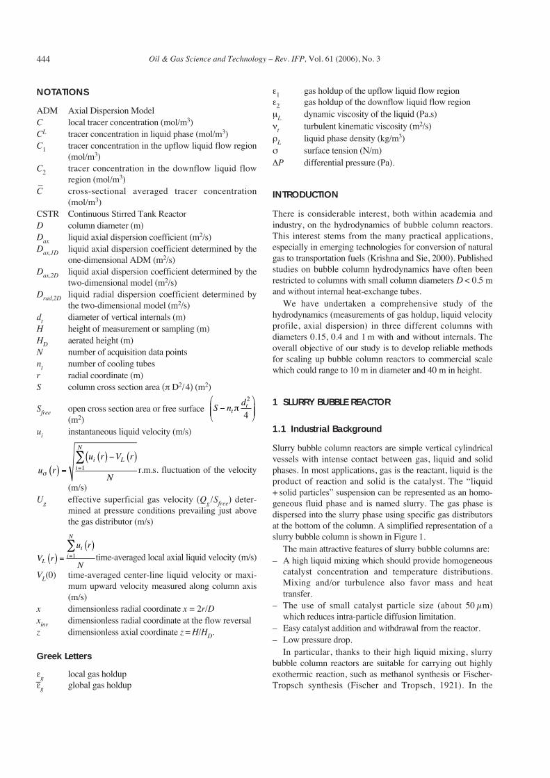
Slurry bubble column reactors are simple vertical cylindricalvessels with intense contact between gas, liquid and solidphases. In most applications, gas is the reactant, liquid is theproduct of reaction and solid is the catalyst. The “liquid+ solid particles” suspension can be represented as an homo-geneous fluid phase and is named slurry. The gas phase isdispersed into the slurry phase using specific gas distributorsat the bottom of the column. A simplified representation of aslurry bubble column is shown in Figure 1.

The main attractive features of slurry bubble columns are:– A high liquid mixing which should provide homogeneous

catalyst concentration and temperature distributions.Mixing and/or turbulence also favor mass and heattransfer.

– The use of small catalyst particle size (about 50 μm)which reduces intra-particle diffusion limitation.

– Easy catalyst addition and withdrawal from the reactor.– Low pressure drop.

In particular, thanks to their high liquid mixing, slurrybubble column reactors are suitable for carrying out highlyexothermic reaction, such as methanol synthesis or Fischer-Tropsch synthesis (Fischer and Tropsch, 1921). In the

V r

u r

NL

ii

N

( ) =( )

=

∑1

u r

u r V r

N

i Li

N

σ ( ) =( ) − ( )(

=

∑1

S nd

tt−

⎛

⎝⎜⎜

⎞

⎠⎟⎟π

2

4

Oil & Gas Science and Technology – Rev. IFP, Vol. 61 (2006), No. 3444

A Forret et al. / Scale Up of Slurry Bubble Reactors

Figure 1

Slurry bubble column scheme.

Fischer-Tropsch process, the reacting gas is a mixture ofhydrogen and carbon monoxide called synthesis gas orshortly syngas. The reaction is heterogeneously catalyzedusing an iron or cobalt based catalyst. To produce gasoil likemolecules, say C16H34, one has to evacuate 16 × 165 kJ permole of cetane. To remove heat from the reacting medium, aslurry reactor equipped with an immersed tubular heatexchanger is an appropriate reactor technology.

Nevertheless, these reactors present also some drawbacks:– The high liquid mixing is detrimental for the conversion

and could generate catalyst attrition. – The separation of fine solid catalyst particles from liquid

products is difficult.– Slurry handling requires careful design to avoid plugging.

In addition, large gas throughputs are involved, requiringthe use of large reactor diameter, typically 5-10 m. Reliablescale-up and design criteria are needed but are still lacking.Our study will therefore focus on the scale-up of hydro-dynamics.

1.2 Phenomenology of a Slurry Bubble Column

The hydrodynamic behavior of bubble columns is stronglydependent on the flow regime (Deckwer et al., 1980).Commercial reactors are usually operated at high gasvelocity, i.e. in the churn turbulent regime. A briefdescription of the flow regimes encountered in bubblecolumns and of flow regime transitions is presented below.

Gas holdup regimes in slurry bubble columns aregenerally investigated by measuring or watching theevolution of the bubble characteristics (bubble shape, sizeand velocity) as a function of operating conditions (gas

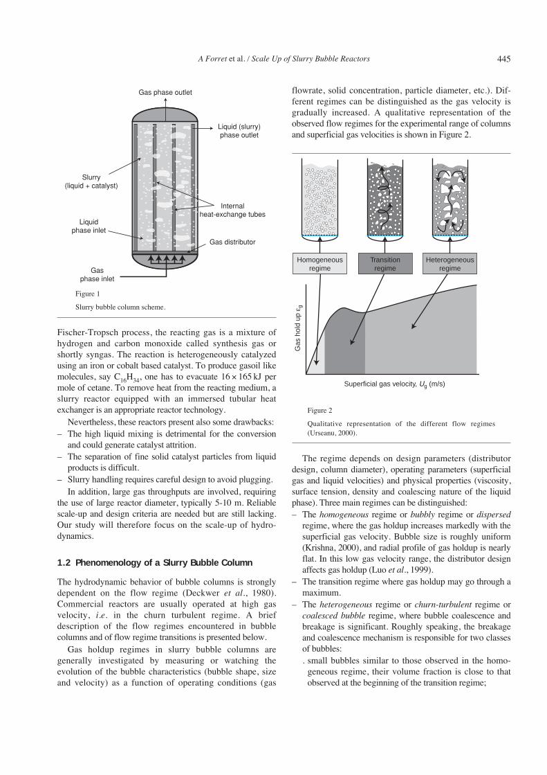
flowrate, solid concentration, particle diameter, etc.). Dif-ferent regimes can be distinguished as the gas velocity isgradually increased. A qualitative representation of theobserved flow regimes for the experimental range of columnsand superficial gas velocities is shown in Figure 2.

Figure 2

Qualitative representation of the different flow regimes(Urseanu, 2000).

The regime depends on design parameters (distributordesign, column diameter), operating parameters (superficialgas and liquid velocities) and physical properties (viscosity,surface tension, density and coalescing nature of the liquidphase). Three main regimes can be distinguished:– The homogeneous regime or bubbly regime or dispersed

regime, where the gas holdup increases markedly with thesuperficial gas velocity. Bubble size is roughly uniform(Krishna, 2000), and radial profile of gas holdup is nearlyflat. In this low gas velocity range, the distributor designaffects gas holdup (Luo et al., 1999).

– The transition regime where gas holdup may go through amaximum.

– The heterogeneous regime or churn-turbulent regime orcoalesced bubble regime, where bubble coalescence andbreakage is significant. Roughly speaking, the breakageand coalescence mechanism is responsible for two classesof bubbles:. small bubbles similar to those observed in the homo-

geneous regime, their volume fraction is close to thatobserved at the beginning of the transition regime;

Superficial gas velocity, Ug (m/s)

Gas

hol

d up

εg

Homogeneousregime

Transitionregime

Heterogeneousregime

445


. large bubbles that move quickly upwards as vaporbubbles in a boiling liquid. The radial profile of gasholdup shows a maximum at the column centre-line,and holdup is nearly zero at the wall (Krishna andEllenberger, 1996; Krishna et al., 1996).

For completeness, the slug regime can be found whensuperficial gas velocity is increased further. The slug regimeis highly unstable. The gas passes through the liquid inintermittent plugs while the liquid near the wall continuouslypulses up and down. This regime is generally limited tocolumns of small diameter.

The domain of industrial interest concerns in particular theheterogeneous regime, characterized by high mass and heattransfers.

2 STATE OF THE ART

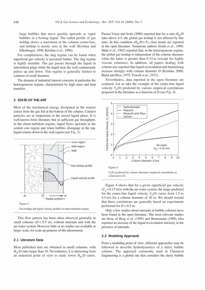
Most of the mechanical energy dissipated in the reactorcomes from the gas fed at the bottom of the column. Catalystparticles are in suspension in the mixed liquid phase. It iswell-known from literature that at sufficient gas throughput,in the churn-turbulent regime, liquid flows upwards in thecentral core region and when bubbles disengage at the top,liquid returns down in the wall region (see Fig. 3).

Figure 3

Gas holdup and liquid velocity profiles in churn turbulent regime.

This flow pattern has been often observed generally insmall columns (D < 0.5 m), without internals and with theair-water system. However little or no studies are available atlarger scale, for scale up purpose of this phenomena.

2.1 Literature Data

Most published data are obtained in small columns, withHD/D ratio larger than 10. Nevertheless, it is interesting froman industrial point of view to study lower HD/D ratios.

Parasu Veera and Joshi (2000) reported that for a ratio HD/Dratio above 4-5, the global gas holdup is not affected by thisratio. In this condition (HD/D > 5), clear trends are reportedin the open literature. Numerous authors (Joshi et al., 1998;Shah et al., 1982) reported that, in the heterogeneous regime,the global gas holdup is independent of the column diameterwhen the latter is greater than 0.15 m (except for highlyviscous solutions). In addition, all papers dealing withcolumn size reported that liquid recirculation and backmixingincrease strongly with column diameter D (Krishna, 2000;Baird and Rice, 1975; Towell et al., 1972).

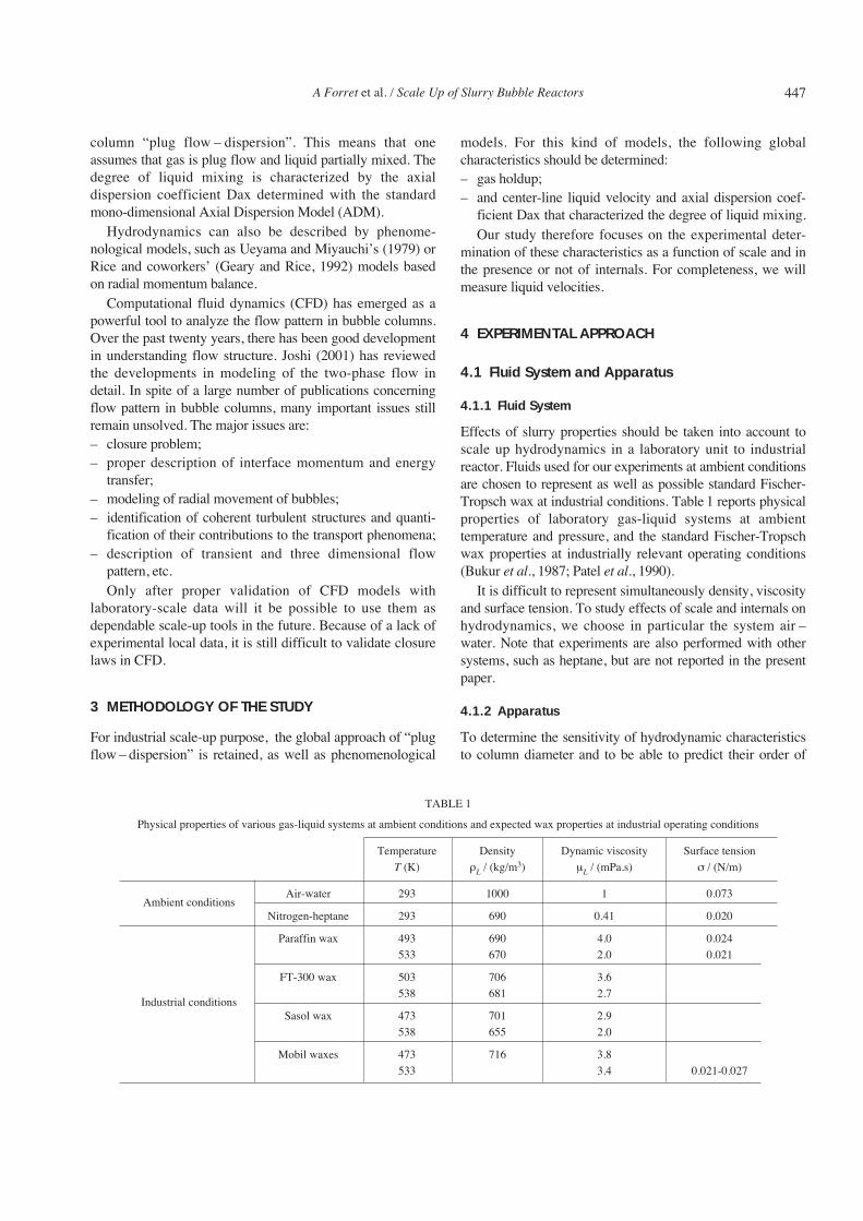
Nevertheless, data reported in the open literature arescattered. Let us take the example of the centre-line liquidvelocity VL(0) predicted by various empirical correlationsproposed in the literature as a function of D (see Fig. 4).

Figure 4

VL(0) predicted by various literature empirical correlations asa function of D.

Figure 4 shows that for a given superficial gas velocity(Ug = 0.15 m/s) with the air-water system, the range predictedfor the centre-line liquid velocity VL(0) varies from 1.5 to4.5 m/s for a column diameter of 10 m. We should remindthat these correlations are generally based on experimentsperformed for D < 0.5 m.

Only a few studies about internals in bubble columns havebeen found in the open literature. The most relevant studiesare those of Berg et al. (1995) and Bernemann (1989) whoreported an increase of the liquid recirculation intensity in thepresence of internals.

2.2 Modeling Approach

From a modeling point of view, different approaches may befollowed to describe hydrodynamics of a slurry bubblecolumn. The approach commonly used in ChemicalEngineering is a global one that considers the slurry bubble

0

1

2

3

4

5

0 1 2 3 4 5 6 7 8 9 10

Cen

tre-

line

liqui

d ve

loci

ty, V

L (0

)(m

/s)

Column diameter D (m)

Air-waterUg = 0.15 m/s

NottenkamperRiquartsMiyauchi and ShyuZehner

-R R

VL (0)

0

Core region

Wall region

Wall

Gas holdup profile

Liquid velocity profile

Radial position t

446


column “plug flow – dispersion”. This means that oneassumes that gas is plug flow and liquid partially mixed. Thedegree of liquid mixing is characterized by the axialdispersion coefficient Dax determined with the standardmono-dimensional Axial Dispersion Model (ADM).

Hydrodynamics can also be described by phenome-nological models, such as Ueyama and Miyauchi’s (1979) orRice and coworkers’ (Geary and Rice, 1992) models basedon radial momentum balance.

Computational fluid dynamics (CFD) has emerged as apowerful tool to analyze the flow pattern in bubble columns.Over the past twenty years, there has been good developmentin understanding flow structure. Joshi (2001) has reviewedthe developments in modeling of the two-phase flow indetail. In spite of a large number of publications concerningflow pattern in bubble columns, many important issues stillremain unsolved. The major issues are:– closure problem;– proper description of interface momentum and energy

transfer;– modeling of radial movement of bubbles;– identification of coherent turbulent structures and quanti-

fication of their contributions to the transport phenomena;– description of transient and three dimensional flow

pattern, etc.Only after proper validation of CFD models with

laboratory-scale data will it be possible to use them asdependable scale-up tools in the future. Because of a lack ofexperimental local data, it is still difficult to validate closurelaws in CFD.

3 METHODOLOGY OF THE STUDY

For industrial scale-up purpose, the global approach of “plugflow – dispersion” is retained, as well as phenomenological

models. For this kind of models, the following globalcharacteristics should be determined:– gas holdup;– and center-line liquid velocity and axial dispersion coef-

ficient Dax that characterized the degree of liquid mixing.Our study therefore focuses on the experimental deter-

mination of these characteristics as a function of scale and inthe presence or not of internals. For completeness, we willmeasure liquid velocities.

4 EXPERIMENTAL APPROACH

4.1 Fluid System and Apparatus

4.1.1 Fluid System

Effects of slurry properties should be taken into account toscale up hydrodynamics in a laboratory unit to industrialreactor. Fluids used for our experiments at ambient conditionsare chosen to represent as well as possible standard Fischer-Tropsch wax at industrial conditions. Table 1 reports physicalproperties of laboratory gas-liquid systems at ambienttemperature and pressure, and the standard Fischer-Tropschwax properties at industrially relevant operating conditions(Bukur et al., 1987; Patel et al., 1990).

It is difficult to represent simultaneously density, viscosityand surface tension. To study effects of scale and internals onhydrodynamics, we choose in particular the system air –water. Note that experiments are also performed with othersystems, such as heptane, but are not reported in the presentpaper.

4.1.2 Apparatus

To determine the sensitivity of hydrodynamic characteristicsto column diameter and to be able to predict their order of

447

TABLE 1

Physical properties of various gas-liquid systems at ambient conditions and expected wax properties at industrial operating conditions

Temperature Density Dynamic viscosity Surface tension

T (K) ρL / (kg/m3) μL / (mPa.s) σ / (N/m)

Ambient conditionsAir-water 293 1000 1 0.073

Nitrogen-heptane 293 690 0.41 0.020

Paraffin wax 493 690 4.0 0.024

533 670 2.0 0.021

FT-300 wax 503 706 3.6

Industrial conditions538 681 2.7

Sasol wax 473 701 2.9

538 655 2.0

Mobil waxes 473 716 3.8

533 3.4 0.021-0.027


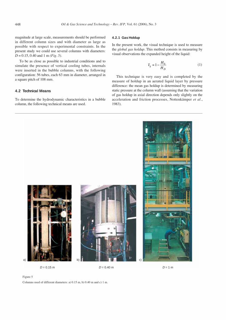
magnitude at large scale, measurements should be performedin different column sizes and with diameter as large aspossible with respect to experimental constraints. In thepresent study we could use several columns with diameters:D = 0.15, 0.40 and 1 m (Fig. 5).

To be as close as possible to industrial conditions and tosimulate the presence of vertical cooling tubes, internalswere inserted in the bubble columns, with the followingconfiguration: 56 tubes, each 63 mm in diameter, arranged ina square pitch of 108 mm.

4.2 Technical Means

To determine the hydrodynamic characteristics in a bubblecolumn, the following technical means are used.

4.2.1 Gas Holdup

In the present work, the visual technique is used to measurethe global gas holdup. This method consists in measuring byvisual observations the expanded height of the liquid:

(1)

This technique is very easy and is completed by themeasure of holdup in an aerated liquid layer by pressuredifference: the mean gas holdup is determined by measuringstatic pressure at the column wall (assuming that the variationof gas holdup in axial direction depends only slightly on theacceleration and friction processes, Nottenkämper et al.,1983).

εgD

H

H= −1 0

448

D = 0.15 m D = 0.40 m D = 1 m

a) b) c)

Figure 5

Columns used of different diameters: a) 0.15 m, b) 0.40 m and c) 1 m.


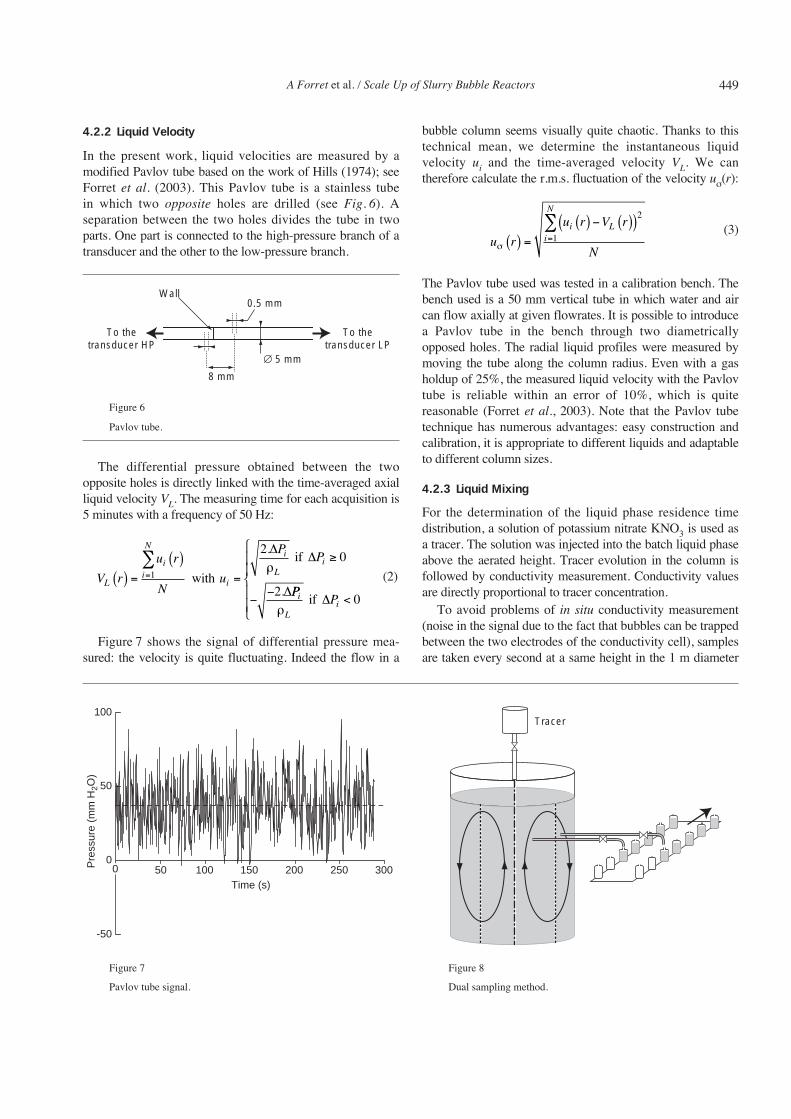
4.2.2 Liquid Velocity

In the present work, liquid velocities are measured by amodified Pavlov tube based on the work of Hills (1974); seeForret et al. (2003). This Pavlov tube is a stainless tubein which two opposite holes are drilled (see Fig. 6). Aseparation between the two holes divides the tube in twoparts. One part is connected to the high-pressure branch of atransducer and the other to the low-pressure branch.

Figure 6

Pavlov tube.

The differential pressure obtained between the twoopposite holes is directly linked with the time-averaged axialliquid velocity VL. The measuring time for each acquisition is5 minutes with a frequency of 50 Hz:

(2)

Figure 7 shows the signal of differential pressure mea-sured: the velocity is quite fluctuating. Indeed the flow in a

bubble column seems visually quite chaotic. Thanks to thistechnical mean, we determine the instantaneous liquidvelocity ui and the time-averaged velocity VL. We cantherefore calculate the r.m.s. fluctuation of the velocity uσ(r):

(3)

The Pavlov tube used was tested in a calibration bench. Thebench used is a 50 mm vertical tube in which water and aircan flow axially at given flowrates. It is possible to introducea Pavlov tube in the bench through two diametricallyopposed holes. The radial liquid profiles were measured bymoving the tube along the column radius. Even with a gasholdup of 25%, the measured liquid velocity with the Pavlovtube is reliable within an error of 10%, which is quitereasonable (Forret et al., 2003). Note that the Pavlov tubetechnique has numerous advantages: easy construction andcalibration, it is appropriate to different liquids and adaptableto different column sizes.

4.2.3 Liquid Mixing

For the determination of the liquid phase residence timedistribution, a solution of potassium nitrate KNO3 is used asa tracer. The solution was injected into the batch liquid phaseabove the aerated height. Tracer evolution in the column isfollowed by conductivity measurement. Conductivity valuesare directly proportional to tracer concentration.

To avoid problems of in situ conductivity measurement(noise in the signal due to the fact that bubbles can be trappedbetween the two electrodes of the conductivity cell), samplesare taken every second at a same height in the 1 m diameter

u r

u r V r

N

i Li

N

σ ( ) =( ) − ( )( )

=

∑ 2

1

V r

u r

Nu

PP

L

ii

N

i

i

Li

( ) =( )

=

≥

−−

=

∑1

20

2with

if.

.

ΔΔ

Δ

ρ

PPPi

Liρ

if Δ <

⎧

⎨

⎪⎪

⎩

⎪⎪ 0

To thetransducer HP

8 mm

Wall0.5 mm

∅ 5 mm

To thetransducer LP

449

-50

0

50

100

50 100 150 200 250 300Time (s)

Pre

ssur

e (m

m H

2O)

0

Tracer

Figure 7

Pavlov tube signal.

Figure 8

Dual sampling method.


column. Conductivity of each sample is then measured.Sampling is performed at two radial positions (one in themiddle of the upflow liquid flow region, the other in themiddle of the downflow liquid flow region) (see Fig. 8).

The two sampling tubes have the same length in order tokeep the same liquid crossing time in each tube.

5 EXPERIMENTAL RESULTS

5.1 Flow Structure of the Stabilized Regionof a Bubble Column

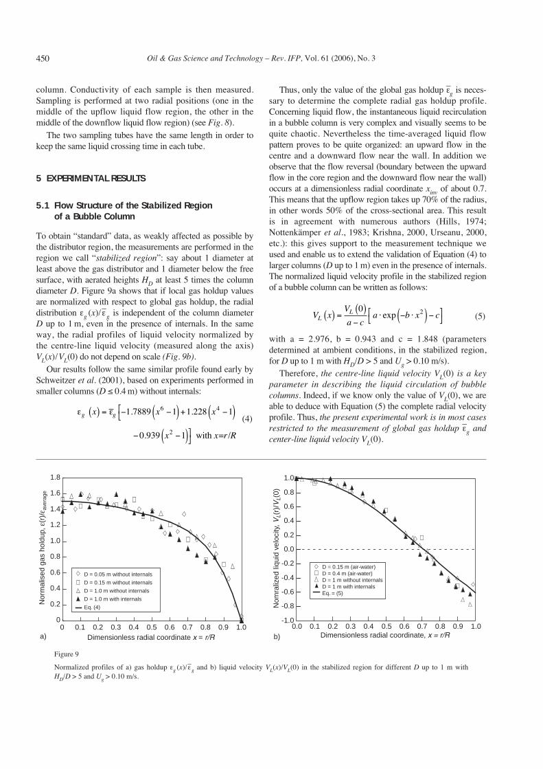
To obtain “standard” data, as weakly affected as possible bythe distributor region, the measurements are performed in theregion we call “stabilized region”: say about 1 diameter atleast above the gas distributor and 1 diameter below the freesurface, with aerated heights HD at least 5 times the columndiameter D. Figure 9a shows that if local gas holdup valuesare normalized with respect to global gas holdup, the radialdistribution εg (x)/ε–g is independent of the column diameterD up to 1 m, even in the presence of internals. In the sameway, the radial profiles of liquid velocity normalized bythe centre-line liquid velocity (measured along the axis)VL(x)/VL(0) do not depend on scale (Fig. 9b).

Our results follow the same similar profile found early bySchweitzer et al. (2001), based on experiments performed insmaller columns (D ≤ 0.4 m) without internals:

(4)

Thus, only the value of the global gas holdup ε–g is neces-sary to determine the complete radial gas holdup profile.Concerning liquid flow, the instantaneous liquid recirculationin a bubble column is very complex and visually seems to bequite chaotic. Nevertheless the time-averaged liquid flowpattern proves to be quite organized: an upward flow in thecentre and a downward flow near the wall. In addition weobserve that the flow reversal (boundary between the upwardflow in the core region and the downward flow near the wall)occurs at a dimensionless radial coordinate xinv of about 0.7.This means that the upflow region takes up 70% of the radius,in other words 50% of the cross-sectional area. This resultis in agreement with numerous authors (Hills, 1974;Nottenkämper et al., 1983; Krishna, 2000, Urseanu, 2000,etc.): this gives support to the measurement technique weused and enable us to extend the validation of Equation (4) tolarger columns (D up to 1 m) even in the presence of internals.The normalized liquid velocity profile in the stabilized regionof a bubble column can be written as follows:

(5)

with a = 2.976, b = 0.943 and c = 1.848 (parametersdetermined at ambient conditions, in the stabilized region,for D up to 1 m with HD/D > 5 and Ug > 0.10 m/s).

Therefore, the centre-line liquid velocity VL(0) is a keyparameter in describing the liquid circulation of bubblecolumns. Indeed, if we know only the value of VL(0), we areable to deduce with Equation (5) the complete radial velocityprofile. Thus, the present experimental work is in most casesrestricted to the measurement of global gas holdup ε–g andcenter-line liquid velocity VL(0).

V xV

a ca b x cL

L( ) =( )−

⋅ − ⋅( ) −⎡⎣

⎤⎦

0 2exp

− −( )⎤⎦0 939 12. x x r Rwith = /

ε εg gx x x( ) = − −( ) + −( )⎡⎣ 1 7889 1 1 228 16 4. .

450

Figure 9

Normalized profiles of a) gas holdup εg (x)/ε–g and b) liquid velocity VL(x)/VL(0) in the stabilized region for different D up to 1 m withHD/D > 5 and Ug > 0.10 m/s.

0

0.2

0.4

0.6

0.8

1.0

1.2

1.4

1.6

1.8

Dimensionless radial coordinate x = r/R0 0.1 0.2 0.3 0.4 0.5 0.6 0.7 0.8 0.9 1.0

D = 0.05 m without internals



D = 1.0 m with internals

Eq. (4)

a)

Nor

mal

ised

gas

hol

dup,

ε(r

)/ε a

vera

ge

-1.0

-0.8

-0.6

-0.4

-0.2

0.0

0.2

0.4

0.6

0.8

1.0

0.0 0.1 0.2 0.3 0.4 0.5 0.6 0.7 0.8 0.9 1.0

Nom

raliz

ed li

quid

vel

ocity

, VL(

r)/V

L(0)

D = 0.15 m (air-water)D = 0.4 m (air-water)D = 1 m without internalsD = 1 m with internalsEq. = (5)

Dimensionless radial coordinate, x = r/Rb)


5.2 Liquid Mixing in a Bubble Column

From a modeling point of view, the liquid mixing can simplybe characterized by an axial dispersion coefficient, deter-mined in this work by the dual-sampling method detailedabove in § 4.2.3. As the cross section of the upflow liquidflow region is equal to the cross section of the downflowliquid flow region and according to the assumption that thetracer concentration is homogeneous in all the cross sectionof the upflow (C1) or downflow (C2) liquid flow region, theaverage tracer concentration is calculated as following:

(6)

where ε1 and ε2 (respectively C1 and C2) are the gas holdups(respectively concentrations) in the upflow and downflowregions. Due to the short time needed for the mixing of thetracer (few seconds), averaging of three dual samplings percross section are performed for each operating condition,at different height elevations. Then, a mono-dimensionaldispersed-plug-flow model (axial dispersion model, ADM) isapplied in order to determine the axial dispersion coefficient.

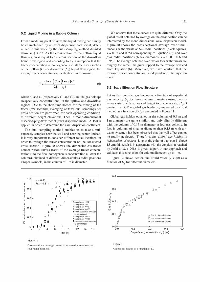
The dual sampling method enables us to take simul-taneously samples near the wall and near the center. Indeed,it is very important to consider different radial locations, inorder to average the tracer concentration on the consideredcross section. Figure 10 shows the dimensionless tracerconcentration curves (ratio of the average tracer concen-tration C

–to the final homogeneous concentration all over the

column), obtained at different dimensionless radial positionsx (open symbols) in the column of 1 m in diameter.

We observe that these curves are quite different. Only theglobal result obtained by average on the cross section can beinterpreted by the mono-dimensional axial dispersion model.Figure 10 shows the cross-sectional average over simul-taneous withdrawals at two radial positions (black squares,x = 0.35 and 0.85) corresponding to Equation (6), and overfour radial positions (black diamonds, x = 0, 0.3, 0.6 and0.95). The average obtained over two or four withdrawals areroughly the same: this gives support to the average deducedfrom Equation (6). Moreover, we have verified that theaveraged tracer concentration is independent of the injectionmode.

5.3 Scale Effect on Flow Structure

Let us first consider gas holdup as a function of superficialgas velocity Ug for three column diameters using the air-water system with an aerated height to diameter ratio HD/Dgreater than 5. The global gas holdup ε–g measured by visualmethod as a function of Ug is presented in Figure 11.

Global gas holdup obtained in the columns of 0.4 m and1 m diameter are quite similar, and only slightly differentwith the column of 0.15 m diameter at low gas velocity. Infact in columns of smaller diameter than 0.15 m with air-water system, it has been observed that the wall effect cannotbe totally neglected. Therefore, the global gas holdup isindependent of scale as long as the column diameter is above15 cm; this result is in agreement with the conclusion reachedby Joshi et al. (1998): it gives support to our approach andvalidates this conclusion for column diameters up to 1 m.

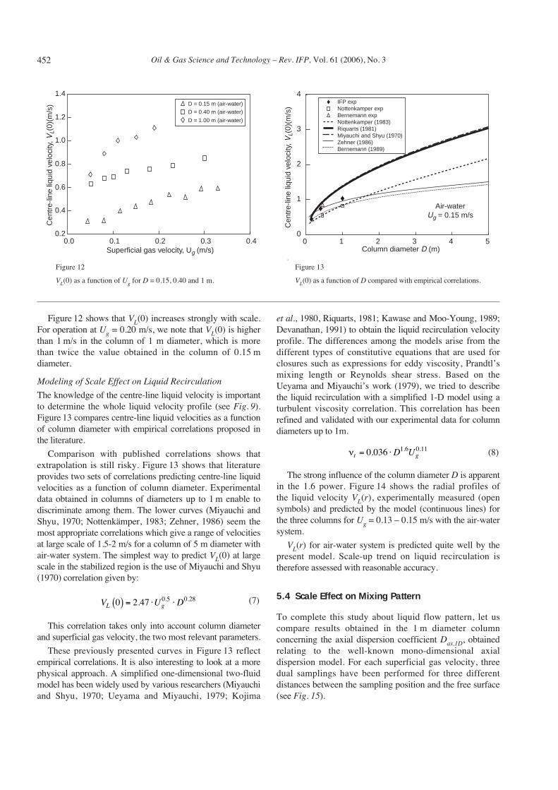
Figure 12 shows center-line liquid velocity VL(0) as afunction of Ug for different diameters.

CC C

g

=−( ) + −( )

−( )1 1

2 11 1 2 2ε ε

ε

451

Figure 10

Cross-sectional averaged tracer concentration over two andfour radial positions.

Figure 11

Global gas holdup as a function of D.

0

0.2

0.4

0.6

0.8

1.0

0 2 4 6 8 10 12 14 16Time (s)

Dim

ensi

onle

ss tr

acer

con

cent

ratio

n

z = 0.41HD = 4.3 m

sampling x = 0.3sampling x = 0sampling x = 0.6sampling x = 0.95cross-sectional average(4 samplings)sampling x = 0.35sampling x = 0.85cross-sectional average(2 samplings)

0.0

0.1

0.2

0.3

0.4

0.0 0.1 0.2 0.3 0.4

D = 0.15 m (air-water)



Gas

hol

dup,

εg



Figure 12 shows that VL(0) increases strongly with scale.For operation at Ug = 0.20 m/s, we note that VL(0) is higherthan 1 m/s in the column of 1 m diameter, which is morethan twice the value obtained in the column of 0.15 mdiameter.

Modeling of Scale Effect on Liquid Recirculation

The knowledge of the centre-line liquid velocity is importantto determine the whole liquid velocity profile (see Fig. 9).Figure 13 compares centre-line liquid velocities as a functionof column diameter with empirical correlations proposed inthe literature.

Comparison with published correlations shows thatextrapolation is still risky. Figure 13 shows that literatureprovides two sets of correlations predicting centre-line liquidvelocities as a function of column diameter. Experimentaldata obtained in columns of diameters up to 1 m enable todiscriminate among them. The lower curves (Miyauchi andShyu, 1970; Nottenkämper, 1983; Zehner, 1986) seem themost appropriate correlations which give a range of velocitiesat large scale of 1.5-2 m/s for a column of 5 m diameter withair-water system. The simplest way to predict VL(0) at largescale in the stabilized region is the use of Miyauchi and Shyu(1970) correlation given by:

(7)

This correlation takes only into account column diameterand superficial gas velocity, the two most relevant parameters.

These previously presented curves in Figure 13 reflectempirical correlations. It is also interesting to look at a morephysical approach. A simplified one-dimensional two-fluidmodel has been widely used by various researchers (Miyauchiand Shyu, 1970; Ueyama and Miyauchi, 1979; Kojima

et al., 1980, Riquarts, 1981; Kawase and Moo-Young, 1989;Devanathan, 1991) to obtain the liquid recirculation velocityprofile. The differences among the models arise from thedifferent types of constitutive equations that are used forclosures such as expressions for eddy viscosity, Prandtl’smixing length or Reynolds shear stress. Based on theUeyama and Miyauchi’s work (1979), we tried to describethe liquid recirculation with a simplified 1-D model using aturbulent viscosity correlation. This correlation has beenrefined and validated with our experimental data for columndiameters up to 1m.

(8)

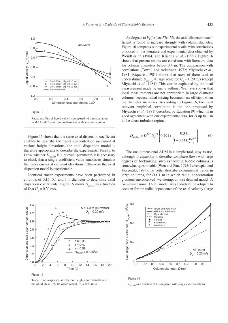
The strong influence of the column diameter D is apparentin the 1.6 power. Figure 14 shows the radial profiles ofthe liquid velocity VL(r), experimentally measured (opensymbols) and predicted by the model (continuous lines) forthe three columns for Ug = 0.13 – 0.15 m/s with the air-watersystem.

VL(r) for air-water system is predicted quite well by thepresent model. Scale-up trend on liquid recirculation istherefore assessed with reasonable accuracy.

5.4 Scale Effect on Mixing Pattern

To complete this study about liquid flow pattern, let uscompare results obtained in the 1 m diameter columnconcerning the axial dispersion coefficient Dax,1D, obtainedrelating to the well-known mono-dimensional axialdispersion model. For each superficial gas velocity, threedual samplings have been performed for three differentdistances between the sampling position and the free surface(see Fig. 15).

νt gD U= ⋅0 036 1 6 0 11. . .

V U DL g0 2 47 0 5 0 28( ) = ⋅ ⋅. . .

452

0.2

0.4

0.6

0.8

1.0

1.2

1.4

0.0 0.1 0.2 0.3 0.4

D = 0.15 m (air-water)D = 0.40 m (air-water)


Cen

tre-

line

liqui

d ve

loci

ty, V

L(0)

(m/s

)


Cen

tre-

line

liqui

d ve

loci

ty, V

L(0)

(m/s

)

0

1

2

3

4

0 1 2 3 4 5Column diameter D (m)

IFP expNottenkamper expBernemann expNottenkamper (1983)Riquarts (1981)Miyauchi and Shyu (1970)Zehner (1986)Bernemann (1989)


Figure 12

VL(0) as a function of Ug for D = 0.15, 0.40 and 1 m.

Figure 13

VL(0) as a function of D compared with empirical correlations.


Figure 14

Radial profiles of liquid velocity compared with recirculationmodel for different column diameters with air-water system.

Figure 15 shows that the same axial dispersion coefficientenables to describe the tracer concentration measured atvarious height elevations: the axial dispersion model istherefore appropriate to describe the experiments. Finally, toknow whether Dax,1D is a relevant parameter, it is necessaryto check that a single coefficient value enables to simulatethe tracer curves at different elevations. Otherwise the axialdispersion model is questionable.

Identical tracer experiments have been performed incolumns of 0.15, 0.4 and 1 m diameter to determine axialdispersion coefficients. Figure 16 shows Dax,1D as a functionof D at Ug = 0.20 m/s.

Analogous to VL(0) (see Fig. 13), the axial dispersion coef-ficient is found to increase strongly with column diameter.Figure 16 compares our experimental results with correlationsproposed in the literature and experimental data obtained byWendt et al. (1984) and Krishna et al. (1999). Figure 16shows that present results are consistent with literature datafor column diameters below 0.4 m. The comparison withcorrelations (Towell and Ackerman, 1972; Miyauchi et al.,1981; Riquarts, 1981) shows that most of them tend tounderestimate Dax,1D at large scale for Ug = 0.20 m/s (exceptMiyauchi et al., 1981). This can be explained by the localmeasurement made by many authors. We have shown thatlocal measurements are not appropriate in large diametercolumns because radial mixing becomes less efficient whenthe diameter increases. According to Figure 16, the mostrelevant empirical correlation is the one proposed byMiyauchi et al. (1981) described by Equation (9) which is ingood agreement with our experimental data, for D up to 1 min the churn turbulent regime.

(9)

The one-dimensional ADM is a simple tool, easy to use,although its capability to describe two-phase flows with largedegrees of backmixing, such as those in bubble columns issomewhat questionable (Wen and Fan, 1975; Levenspiel andFitzgerald, 1983). To better describe experimental trends inlarge columns, for D ≥ 1 m in which radial concentrationgradients are observed, we attempt a more detailed model. Atwo-dimensional (2-D) model was therefore developed toaccount for the radial dependence of the axial velocity (large

Dax, D13 2 1 4

1 2 20 291

0 341

1 0 54= +

−( )

⎛

⎝

D UU

g

g

/ /

/.

.

.

⎜⎜⎜⎜

⎞

⎠

⎟⎟⎟

-1.2

-0.8

-0.4

0.0

0.4

0.8

1.2

0.0 0.2 0.4 0.6 0.8 1.0

Air-water

Liqu

id v

eloc

ity, V

L(r)

(m/s

)

Dimensionless coordinate, 2r/D

D = 0.15 m ; Ug = 0.15 m/sD = 0.40 m ; Ug = 0.13 m/sD = 1.00 m ; Ug = 0.15 m/sPresent model

453

Figure 15

Tracer time responses at different heights and validation ofthe ADM (D = 1 m, air-water system, Ug = 0.20 m/s).

Figure 16

Dax,1D as a function of D compared with empirical correlations.

0.0

0.2

0.4

0.6

0.8

1.0

1.2

1.4

0 2 4 6 8 10 12 14 16 18 20

Dim

ensi

onle

ss s

alt t

race

r co

ncen

trat

ion

z = 0.33z = 0.42z = 0.59Dax,1D = 0.6 m2/s

D = 1.0 m (air-water)Ug = 0.20 m/s

Time (s)

0

0.2

0.4

0.6

0.1 0.2 0.3 0.4 0.5 0.6 0.7 0.8 0.9 1

Axi

al d

ispe

rsio

n co

effic

ient

, Dax

,1D (

m2 /

s)


Column diameter, D (m)

Towell and AckermanHikita and KikukawaMiyauchi et al.RiquartsIFP exp.Krishna exp.Wendt exp


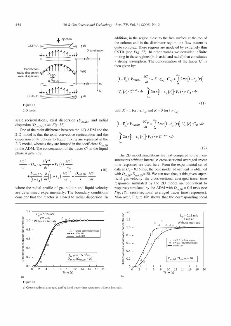
Figure 17

2-D model.

scale recirculation), axial dispersion (Dax,2D) and radialdispersion (Drad,2D) (see Fig. 17).

One of the main difference between the 1-D ADM and the2-D model is that the axial convective recirculation and thedispersion contributions to liquid mixing are separated in the2-D model, whereas they are lumped in the coefficient Dax,1Din the ADM. The concentration of the tracer CL in the liquidphase is given by:

(10)

where the radial profile of gas holdup and liquid velocityare determined experimentally. The boundary conditionsconsider that the reactor is closed to radial dispersion. In

addition, in the region close to the free surface at the top ofthe column and in the distributor region, the flow pattern isquite complex. These regions are modeled by extremely thinCSTR (see Fig. 17). In other words we consider infinitemixing in these regions (both axial and radial) that constitutesa strong assumption. The concentration of the tracer CL isthen given by:

(11)

with K = 1 for t ≤ tinj and K = 0 for t > tinj.

(12)

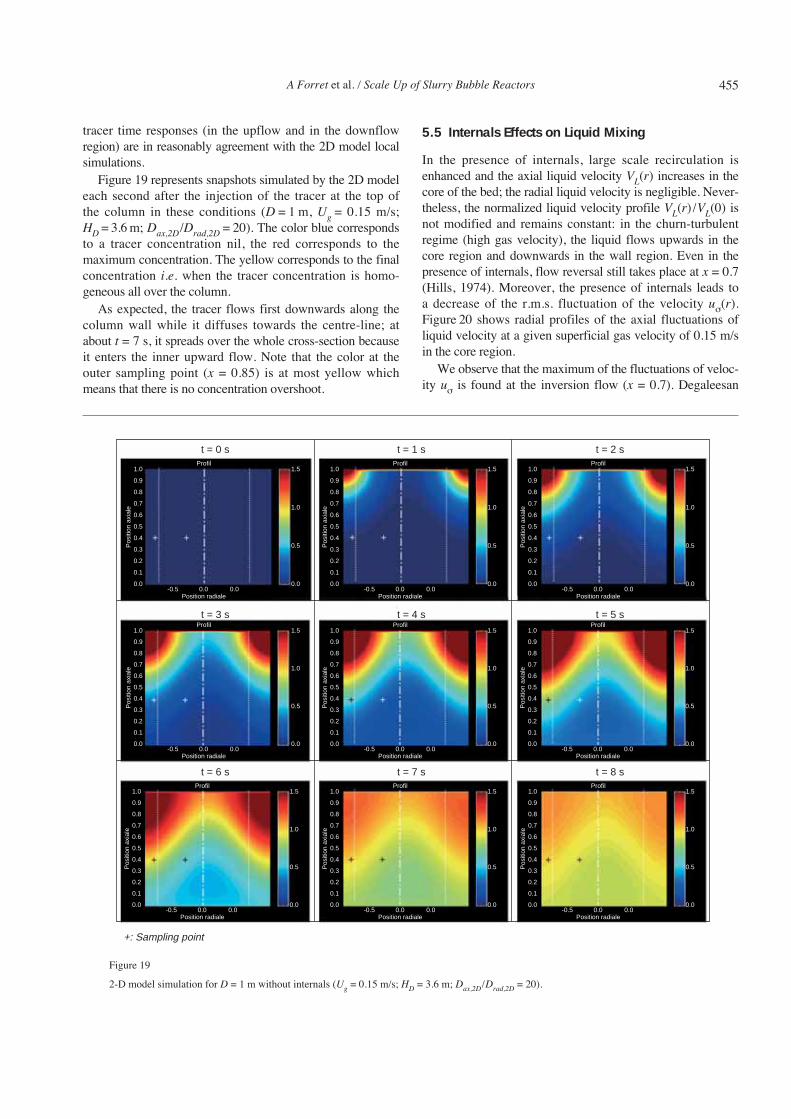
The 2D model simulations are first compared to the mea-surements without internals: cross-sectional averaged tracertime responses are used here. From the experimental set ofdata at Ug = 0.15 m/s, the best model adjustment is obtainedwith Dax,2D/Drad,2D = 20. We can note that, at this given super-ficial gas velocity, the cross-sectional averaged tracer timeresponses simulated by the 2D model are equivalent toresponses simulated by the ADM with Dax,1D = 0.5 m2/s (seeFig. 18a: cross-sectional averaged tracer time responses).Moreover, Figure 18b shows that the corresponding local

1 2 1−( ) ⋅ ⋅∂∂

= − ( )⎡⎣ ⎤⎦⋅ ( ) ⋅ε π εg CSTRBB

g L BVC

tr r V r C ⋅⋅

− − ( )⎡⎣ ⎤⎦⋅ ( ) ⋅ ⋅

∫

=

dr

r r V r C dr

r

g Liz nz

r

inv

i

0

2 1π εnnv

Rr

∫

1 2 1−( ) ⋅ ⋅∂∂

= ⋅ ⋅ + − ( )⎡ε π εg CSTRAA

inj inj gVC

tK q C r r⎣⎣ ⎤⎦

⋅ ( ) ⋅ ⋅ − − ( )⎡⎣ ⎤⎦⋅

∫

=

0

2 1

r

L g L

inv

V r C dr r r Viz 1 π ε rr C drAr

r

inv

R

( ) ⋅ ⋅∫

∂∂

=∂

∂− ( ) ∂

∂

+−

C

t

C

zV r

C

z

L L

L

L

D

D

ax, D

rad, D

2

2

2

2

1

. .

εggg

L L

r

C

r r

C

r( )∂∂

−( ) ∂∂

⎛

⎝⎜⎜

⎞

⎠⎟⎟+

∂∂

. . .1 εDrad, D2

Injection

iz

1

nz

dz

dz

dz

dz

Convectionradial dispersionaxial dispersion

Discretization

VL(r)

CSTR B

CSTR A

Drad,2D

Dax ,2D

454

Figure 18

a) Cross-sectional averaged and b) local tracer time responses without internals.

0.0

0.2

0.4

0.6

0.8

1.0

1.2

0 2 4 6 8 10 12 14 16 18 20Time (s)

Dim

ensi

onle

ss tr

acer

con

cent

ratio

n

Ug = 0.15 m/sz = 0.42

Without internals

Dax,1D = 0.5 m2/sDax,1D /Drad,2D = 20

Cross sectional averageADM 1DModel 2D

a)

0

0.2

0.4

0.6

0.8

1.0

1.2

1.4

0 2 4 6 8 10 12 14 16 18 20Time (s)

Dim

ensi

onle

ss lo

cal t

race

r co

ncen

trat

ion

Ug = 0.15 m/sz = 0.42

Without internals

Dax,2D /Drad,2D = 20

x = 0.3 (upflow region)x = 0.8 (downflow region)model 2D

b)


tracer time responses (in the upflow and in the downflowregion) are in reasonably agreement with the 2D model localsimulations.

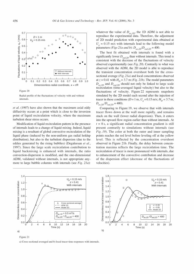
Figure 19 represents snapshots simulated by the 2D modeleach second after the injection of the tracer at the top ofthe column in these conditions (D = 1 m, Ug = 0.15 m/s;HD = 3.6 m; Dax,2D/Drad,2D = 20). The color blue correspondsto a tracer concentration nil, the red corresponds to themaximum concentration. The yellow corresponds to the finalconcentration i.e. when the tracer concentration is homo-geneous all over the column.

As expected, the tracer flows first downwards along thecolumn wall while it diffuses towards the centre-line; atabout t = 7 s, it spreads over the whole cross-section becauseit enters the inner upward flow. Note that the color at theouter sampling point (x = 0.85) is at most yellow whichmeans that there is no concentration overshoot.

5.5 Internals Effects on Liquid Mixing

In the presence of internals, large scale recirculation isenhanced and the axial liquid velocity VL(r) increases in thecore of the bed; the radial liquid velocity is negligible. Never-theless, the normalized liquid velocity profile VL(r) /VL(0) isnot modified and remains constant: in the churn-turbulentregime (high gas velocity), the liquid flows upwards in thecore region and downwards in the wall region. Even in thepresence of internals, flow reversal still takes place at x = 0.7(Hills, 1974). Moreover, the presence of internals leads toa decrease of the r.m.s. fluctuation of the velocity uσ(r).Figure 20 shows radial profiles of the axial fluctuations ofliquid velocity at a given superficial gas velocity of 0.15 m/sin the core region.

We observe that the maximum of the fluctuations of veloc-ity uσ is found at the inversion flow (x = 0.7). Degaleesan

455

1.0

0.9

0.8

0.7

0.6

0.5

0.4

0.3

0.2

0.1

0.0

1.5

1.0

0.5

0.0-0.5 0.0

Position radiale

Pos

ition

axi

ale

Profil

0.0

1.0

0.9

0.8

0.7

0.6

0.5

0.4

0.3

0.2

0.1

0.0

1.5

1.0

0.5

0.0-0.5 0.0

Position radiale

Pos

ition

axi

ale

Profil

0.0

1.0

0.9

0.8

0.7

0.6

0.5

0.4

0.3

0.2

0.1

0.0

1.5

1.0

0.5

0.0-0.5 0.0

Position radiale

Pos

ition

axi

ale

Profil

0.0

1.0

0.9

0.8

0.7

0.6

0.5

0.4

0.3

0.2

0.1

0.0

1.5

1.0

0.5

0.0-0.5 0.0

Position radiale

Pos

ition

axi

ale

Profil

0.0

1.0

0.9

0.8

0.7

0.6

0.5

0.4

0.3

0.2

0.1

0.0

1.5

1.0

0.5

0.0-0.5 0.0

Position radiale

Pos

ition

axi

ale

Profil

0.0

1.0

0.9

0.8

0.7

0.6

0.5

0.4

0.3

0.2

0.1

0.0

1.5

1.0

0.5

0.0-0.5 0.0

Position radiale

Pos

ition

axi

ale

Profil

0.0

1.0

0.9

0.8

0.7

0.6

0.5

0.4

0.3

0.2

0.1

0.0

1.5

1.0

0.5

0.0-0.5 0.0

Position radiale

Pos

ition

axi

ale

Profil

0.0

1.0

0.9

0.8

0.7

0.6

0.5

0.4

0.3

0.2

0.1

0.0

1.5

1.0

0.5

0.0-0.5 0.0

Position radiale

Pos

ition

axi

ale

Profil

0.0

1.0

0.9

0.8

0.7

0.6

0.5

0.4

0.3

0.2

0.1

0.0

1.5

1.0

0.5

0.0-0.5 0.0

Position radiale

Pos

ition

axi

ale

Profil

0.0

t = 0 s

t = 3 s

t = 6 s

t = 1 s

t = 4 s

t = 7 s

t = 2 s

t = 5 s

t = 8 s

+: Sampling point

Figure 19

2-D model simulation for D = 1 m without internals (Ug = 0.15 m/s; HD = 3.6 m; Dax,2D/Drad,2D = 20).


Figure 20

Radial profile of the fluctuations of velocity with and withoutinternals.

et al. (1997) have also shown that the maximum axial eddydiffusivity occurs at a point which is close to the inversionpoint of liquid recirculation velocity, where the maximumturbulent shear stress occurs.

Modification of liquid recirculation pattern in the presenceof internals leads to a change of liquid mixing. Indeed, liquidmixing is a resultant of global convective recirculation of theliquid phase (induced by the non-uniform gas radial holdupdistribution), but also to the turbulent dispersion (due to theeddies generated by the rising bubbles) (Degaleesan et al.,1997). Since the large scale recirculation contribution toliquid backmixing is enhanced with internals, the ratioconvection-dispersion is modified, and the one-dimensionalADM, validated without internals, is not appropriate any-more to large bubble columns with internals (see Fig. 21a):

whatever the value of Dax,1D, the 1D ADM is not able toreproduce the experimental data. Therefore, the adjustmentof 2D model prediction with experimental data obtained atUg = 0.15 m/s with internals lead to the following modelparameters (Figs 21a and b): Dax,2D/Drad,2D = 400.

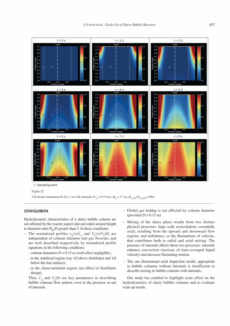
The best fit obtained with internals is found with asignificantly lower Drad,2D than without internals. This trend isconsistent with the decrease of the fluctuations of velocityobserved experimentally (see Fig. 20). Contrarily to what wasobserved with the ADM, the 2D model is able to reproducethe transient concentration overshoot both for the cross-sectional average (Fig. 21a) and local concentrations observedat z = 0.41 with HD = 3.7 m (Fig. 21b). The model parametersDax,2D and Drad,2D should not only be linked to large scalerecirculation (time-averaged liquid velocity) but also to thefluctuations of velocity. Figure 22 represents snapshotssimulated by the 2D model each second after the injection oftracer in these conditions (D = 1 m, Ug = 0.15 m/s; HD = 3.7 m;Dax,2D/Drad,2D = 400).

Comparing to Figure 19, we observe that with internalstracer flows down at the wall more rapidly, and remainsstuck on the wall (lower radial dispersion). Then, it entersinto the upward flow region earlier than without internals. Att = 8 s, a significant radial concentration gradient is stillpresent contrarily to simulations without internals (seeFig. 19). The color at both the outer and inner samplingpoints reaches the red level before leveling off at the yellowlevel. This is reflected by the concentration overshootobserved in Figure 21b. Finally, the delay between concen-tration maxima reflects the large recirculation time. Therecirculation of tracer is more pronounced with internals, dueto enhancement of the convective contribution and decreaseof the dispersion effect (decrease of the fluctuations ofvelocities).

0.0

0.1

0.2

0.3

0.4

0.5

0.6

0.7

0 0.1 0.2 0.3 0.4 0.5 0.6 0.7 0.8 0.9 1.0

Without internalsWith internals

Flu

ctua

tions

of l

iqui

d ve

loci

ty, u

σ / (

m/s

)

Dimensionless radial coordinate, x = r/R

D = 1 mUg = 0.15 m/s

456

Figure 21

a) Cross-sectional averaged and b) local tracer time responses with internals.

0.0

0.2

0.4

0.6

0.8

1.0

1.2

1.4

0 2 4 6 8 10 12 14 16 18 20Time (s)

Dim

ensi

onle

ss tr

acer

con

cent

ratio

n

a)

Ug = 0.15 m/sz = 0.41

With internals

Cross sectional averageADM 1DModel 2D

Dax,1D = 0.5 m2/sDax,2D / Drad,2D = 400

0.0

0.2

0.4

0.6

0.8

1.0

1.2

1.4

1.6

1.8

0 2 4 6 8 10 12 14 16 18 20Time (s)

Dim

ensi

onle

ss lo

cal t

race

r co

ncen

trat

ion

b)

Ug = 0.15 m/sz = 0.41

With internals

Dax,2D /Drad,2D = 400

x = 0.35x = 0.85Model 2D


CONCLUSION

Hydrodynamic characteristics of a slurry bubble column arenot affected by the reactor aspect ratio provided aerated heightto diameter ratio HD/D greater than 5. In these conditions:– The normalized profiles εg(x)/ε–g and VL(x)/VL(0) are

independent of column diameter and gas flowrate, andare well described respectively by normalized profileequations in the following conditions:. column diameters D > 0.15 m (wall effect negligible);. in the stabilized region (say 1D above distributor and 1D

below the free surface);. in the churn-turbulent regime (no effect of distributor

design).Thus, ε–g and VL(0) are key parameters in describingbubble columns flow pattern, even in the presence or notof internals.

– Global gas holdup is not affected by column diameter(provided D > 0.15 m).

– Mixing of the slurry phase results from two distinctphysical processes: large scale recirculations, essentiallyaxial, resulting from the upward and downward flowregions; and turbulence, or the fluctuations of velocity,that contributes both to radial and axial mixing. Thepresence of internals affects these two processes: internalsenhance convection (increase of time-averaged liquidvelocity) and decrease fluctuating motion.

– The one dimensional axial dispersion model, appropriatein bubble columns without internals is insufficient todescribe mixing in bubble columns with internals.

Our study has enabled to highlight scale effect on thehydrodynamics of slurry bubble columns and to evaluatescale up trends.

457

1.0

0.9

0.8

0.7

0.6

0.5

0.4

0.3

0.2

0.1

0.0

1.5

1.0

0.5

0.0-0.5 0.0

Position radiale

Pos

ition

axi

ale

Profil

0.0

1.0

0.9

0.8

0.7

0.6

0.5

0.4

0.3

0.2

0.1

0.0

1.5

1.0

0.5

0.0-0.5 0.0

Position radiale

Pos

ition

axi

ale

Profil

0.0

1.0

0.9

0.8

0.7

0.6

0.5

0.4

0.3

0.2

0.1

0.0

1.5

1.0

0.5

0.0-0.5 0.0

Position radiale

Pos

ition

axi

ale

Profil

0.0

1.0

0.9

0.8

0.7

0.6

0.5

0.4

0.3

0.2

0.1

0.0

1.5

1.0

0.5

0.0-0.5 0.0

Position radiale

Pos

ition

axi

ale

Profil

0.0

1.0

0.9

0.8

0.7

0.6

0.5

0.4

0.3

0.2

0.1

0.0

1.5

1.0

0.5

0.0-0.5 0.0

Position radiale

Pos

ition

axi

ale

Profil

0.0

1.0

0.9

0.8

0.7

0.6

0.5

0.4

0.3

0.2

0.1

0.0

1.5

1.0

0.5

0.0-0.5 0.0

Position radiale

Pos

ition

axi

ale

Profil

0.0

1.0

0.9

0.8

0.7

0.6

0.5

0.4

0.3

0.2

0.1

0.0

1.5

1.0

0.5

0.0-0.5 0.0

Position radiale

Pos

ition

axi

ale

Profil

0.0

1.0

0.9

0.8

0.7

0.6

0.5

0.4

0.3

0.2

0.1

0.0

1.5

1.0

0.5

0.0-0.5 0.0

Position radiale

Pos

ition

axi

ale

Profil

0.0

1.0

0.9

0.8

0.7

0.6

0.5

0.4

0.3

0.2

0.1

0.0

1.5

1.0

0.5

0.0-0.5 0.0

Position radiale

Pos

ition

axi

ale

Profil

0.0

t = 0 s

t = 3 s

t = 6 s

t = 1 s

t = 4 s

t = 7 s

t = 2 s

t = 5 s

t = 8 s

+: Sampling point

Figure 22

2-D model simulation for D = 1 m with internals (Ug = 0.15 m/s; HD = 3.7 m; Dax,2D/Drad,2D = 400).


REFERENCES

Baird, M.H. and Rice, R.G. (1975) Axial Dispersion in LargeUnbaffled Columns. Chem. Eng. J., 9, 171-174.

Berg, S. and Schlüter, S. (1995) Rückvermischung in blasen-säulen mit einbauten. Chem. Ing. Tech., 67, 3, 289-299.

Bernemann, K. (1989) Zur fluiddynamik und zum vermis-chungsverhalten der flüssigen phase in blasensäulen mitlängsangeströmten rohrbündeln (Hydrodynamics of the LiquidPhase in Bubble Columns with internals). Dissertation, Univer-sität Dortmund.

Bukur, D.B., Patel, S.A. and Matheo, R. (1987) HydrodynamicStudies in Fischer-Tropsch Derived Waxes in a Bubble Column.Chem. Eng. Comm., 60, 63-78.

Deckwer, W.D., Louisi, Y., Zaidi, A. and Ralek, M. (1980)Hydrodynamic Properties of the Fischer-Tropsch Slurry Process.Ind. Eng. Chem. Proc. Des. Dev., 19, 699-708.

Degaleesan, S., Dudukovic, M.P., Toseland, B.A. and Bhatt, B.L.(1997) A Two-Compartment Convective-Diffusion Model forSlurry Bubble Column Reactors. Ind. Eng. Chem. Res., 36, 4670-4680.

Devanathan, N. (1991) Investigation of Liquid Hydrodynamics inBubble Columns via a Computer Automated Radioactive ParticleTracking (CARPT). Ph.D. Thesis, Washington University, SaintLouis, Missouri, USA.

Fischer, F. and Tropsch, H. (1921) Synthesis of Methanol fromCO and H2. French Patent 540, 543.

Forret, A., Schweitzer, J.M., Gauthier, T., Krishna, R. andSchweich, D. (2003) Influence of Scale on the Hydrodynamics ofBubble Column Reactors: An Experimental Study in Columns of0.1, 0.4 and 1 m Diameters. Chem. Eng. Sci., 58, 719-724.

Geary, N.W. and Rice, R.G. (1992) Circulation and Scale-Up inBubble Columns. AIChE J., 38, 1, 76-82.

Hills, J.H. (1974) Radial Non-Uniformity of Velocity andVoidage in a Bubble Column. Trans. Inst. Chem. Eng., 52, 1-9.

Joshi, J.B., Parasu Veera, U., Prasad, Ch.V., Phanikumar, D.V.,Deshphande, N.S., Thakre, S.S. and Thorat, B.N. (1998) GasHold-Up Structure in Bubble Column Reactors. PINSA Reviewarticle, 64, A, 4, 441-567.

Joshi, J.B. (2001) Computational Flow Modelling and Design ofBubble Column Reactors. Chem. Eng. Sci., 56, 5893-5933.

Kawase, Y. and Moo-Young, M. (1989) Turbulence Intensity inBubble Columns. Chem. Eng. J., 40, 1, 55-58.

Kojima, E., Unno, H., Sato, Y., Chida, T., Imai, H., Endo, K.,Inoue, I., Kobayashi, J., Kaji, H., Nakanishi, H. and Yamamoto,K. (1980) Liquid Phase Velocity in a 5.5 m Diameter BubbleColumn. Journal of Chemical Engineering of Japan, 13, 1, 16-21.

Krishna, R. and Ellenberger, J. (1996) Gas Holdup in BubbleColumn Reactors Operating in the Churn-Turbulent Regime.AIChE J., 42, 2627-2634.

Krishna, R, Ellenberger, J. and Sie, S.T. (1996) Reactor Devel-opment for Conversion of Natural Gas to Liquid Fuels: a Scale-Up Strategy Relying on Hydrodynamics Analogies. Chem. Eng.Sci., 51, 5041-2050.

Krishna, R., Urseanu, M.I., Van Baten, J.M. and Ellenberger, J.(1999) Influence of Scale on the Hydrodynamics of BubbleColumns Operating in the Churn-Turbulent Regime: Experimentsvs. Eulerian Simulations. Chem. Eng. Sci., 54, 4903-4911.

Krishna, R. (2000) A Scale-up Strategy for a Commercial ScaleBubble Column Slurry Reactor for Fischer-Tropsch Synthesis.Oil & Gas Science and Technology – Rev. IFP, 55, 4, 359-393.

Krishna R. and Sie. S.T. (2000) Selection, Design and Scale-UpAspects of Fischer-Tropsch Reactors. Fuel Processing Technol-ogy, 64, 73-105.

Levenspiel, O. and Fitzgerald, T.J. (1983) A Warning on theMisuse of the Dispersion Model. Chem. Eng. Sci., 38, 489.

Luo, X., Lee, D.J., Lau, R., Yang, G.Q. and Fan, L.S. (1999)Maximum Stable Bubble Size and Gas Holdup in High-pressureSlurry Bubble Columns. AIChE J., 45, 4, 665-680.

Miyauchi, T. and Shyu, C.N. (1970) Flow of Fluid in Gas BubbleColumns. Kagaku Kogaku, 34, 958-964.

Nottenkämper, R., Steiff, A. and Weinspach, P.M. (1983) Exper-imental Investigation of Hydrodynamics of Bubble Columns.Ger. Chem. Eng., 6, 147-155.

Parasu Veera, U. and Joshi, J.B. (2000) Measurement of GasHoldup Profiles in Bubble Column by Gamma Ray Tomography,Effect of Liquid Phase Properties. Trans IChemE, 78, Part A,425-434.

Patel, S.A., Daly, J.G. and Bukur, D.B. (1990) Bubble-SizeDistribution in Fischer-Tropsch Derived Waxes in BubbleColumn. AIChE J., 36, 1, 93-105.

Riquarts, H.P. (1981) A Physical Model for Axial Mixing ofthe Liquid Phase for Heterogeneous Flow Regime in BubbleColumns. German Chemical Engineering, 4, 18-23.

Schweitzer, J.M., Bayle, J. and Gauthier, T. (2001) Local GasHold-Up Measurements in Fluidized Bed and Slurry BubbleColumn. Chem. Eng. Sci., 56, 1103-1110.

Shah, Y.T., Kelkar, B.G., Godbole, S.P. and Deckwer, W.D.(1982) Design Parameters Estimations for Bubble ColumnReactors. AIChE J., 28, 353-379.

Towell, G.D. and Ackerman, G.H. (1972) Axial Mixing of Liquidand Gas in Large Bubble Reactors. Proceeding of 2nd InternationalSymposium Chem. React. Eng., Amsterdam, The Netherlands,B3.1-B3.13.

Ueyama, K. and Miyauchi, T. (1979) Properties of RecirculatingTurbulent Two Phase Flow in Gas Bubble Columns. AIChE J.,25, 2, 258-266.

Urseanu, M.I. (2000) Scaling Up Bubble Column Reactors. Ph.D.Thesis, University of Amsterdam, The Netherlands.

Wen, C.Y. and Fan, L.T. (1975) Models for Flow Systems andChemical Reactors, Dekker, New York.

Wendt, R., Steiff, A. and Weinspach, P.M. (1984) Liquid PhaseDispersion in Bubble Columns. Ger. Chem. Eng., 7, 267-273.

Zehner, P. (1986) Momentum, Mass and Heat Transfer in BubbleColumns, Part 1: Flow Model of the Bubble Column and LiquidVelocities. Int. Chem. Eng., 41, 1969-1977.

Final manuscript received in January 2006

458

Copyright © 2006 Institut français du pétrolePermission to make digital or hard copies of part or all of this work for personal or classroom use is granted without fee provided that copies are not madeor distributed for profit or commercial advantage and that copies bear this notice and the full citation on the first page. Copyrights for components of thiswork owned by others than IFP must be honored. Abstracting with credit is permitted. To copy otherwise, to republish, to post on servers, or to redistributeto lists, requires prior specific permission and/or a fee: Request permission from Documentation, Institut français du pétrole, fax. +33 1 47 52 70 78, or [email protected].

Documents

Scale Up of Slurry Bubble Reactors