Scale-up vs Scale-out for Hadoop: Time to rethink?

Raja Appuswamy∗, Christos Gkantsidis, Dushyanth Narayanan,Orion Hodson, and Antony Rowstron

Microsoft Research, Cambridge, UK

AbstractIn the last decade we have seen a huge deployment ofcheap clusters to run data analytics workloads. The con-ventional wisdom in industry and academia is that scal-ing out using a cluster of commodity machines is betterfor these workloads than scaling up by adding more re-sources to a single server. Popular analytics infrastruc-tures such as Hadoop are aimed at such a cluster scale-out environment.

Is this the right approach? Our measurements as wellas other recent work shows that the majority of real-world analytic jobs process less than 100 GB of input,but popular infrastructures such as Hadoop/MapReducewere originally designed for petascale processing. Weclaim that a single “scale-up” server can process each ofthese jobs and do as well or better than a cluster in termsof performance, cost, power, and server density. Wepresent an evaluation across 11 representative Hadoopjobs that shows scale-up to be competitive in all casesand significantly better in some cases, than scale-out. Toachieve that performance, we describe several modifica-tions to the Hadoop runtime that target scale-up config-uration. These changes are transparent, do not requireany changes to application code, and do not compro-mise scale-out performance; at the same time our evalu-ation shows that they do significantly improve Hadoop’sscale-up performance.

∗ Work done while on internship from Vrije Universiteit Amster-dam

Copyright c© 2013 by the Association for Computing Machinery, Inc.(ACM). Permission to make digital or hard copies of portions of thiswork for personal or classroom use is granted without fee providedthat the copies are not made or distributed for profit or commercial ad-vantage and that copies bear this notice and the full citation on the firstpage in print or the first screen in digital media. Copyrights for com-ponents of this work owned by others than ACM must be honored.Abstracting with credit is permitted. To copy otherwise, to republish,to post on servers, or to redistribute to lists, requires prior specific per-mission and/or a fee.

SoCC’13, 1–3 Oct. 2013, Santa Clara, California, USA.ACM 978-1-4503-2428-1.http://dx.doi.org/10.1145/2523616.2523629

1 IntroductionData analytics, and in particular, MapReduce [14] andHadoop [4] have become synonymous with the use ofcheap commodity clusters using a distributed file sys-tem that utilizes cheap unreliable local disks. This is thestandard scale-out thinking that has underpinned the in-frastructure of many companies. Clearly large clustersof commodity servers are the most cost-effective way toprocess exabytes, petabytes, or multi-terabytes of data.Nevertheless, we ask: is it time to reconsider the scale-out versus scale-up question?

First, evidence suggests that the majority of analyticsjobs do not process huge data sets. For example, at leasttwo analytics production clusters (at Microsoft and Ya-hoo) have median job input sizes under 14 GB [16, 28],and 90% of jobs on a Facebook cluster have input sizesunder 100 GB [2].

Second, hardware price trends are beginning tochange performance points. Today’s servers can afford-ably hold 100s of GB of DRAM and 32 cores on a quadsocket motherboard with multiple high-bandwidth mem-ory channels per socket. DRAM is now very cheap, with16 GB DIMMs costing around $130, meaning 192 GBcosts less than half the price of a dual-socket server and512 GB costs 20% the price of a high-end quad-socketserver. Storage bottlenecks can be removed by usingSSDs or with a scalable storage back-end such as Ama-zon S3 [1] or Azure Storage [9, 31]. The commoditiza-tion of SSDs means that $2,000 can build a storage arraywith multiple GB/s of throughput. Thus a scale-up servercan now have substantial CPU, memory, and storage I/Oresources and at the same time avoid the communicationoverheads of a scale-out solution. Moore’s law contin-ues to improve many of these technologies, at least forthe immediate future.

In this paper, we ask whether it is better to scale upusing a well-provisioned single server or to scale outusing a commodity cluster. For the world of analyticsin general and Hadoop MapReduce in particular, this isan important question. Today the default assumption forHadoop jobs is that scale-out is the only configuration

that matters. Scale-up performance is ignored and in factHadoop performs poorly in a scale-up scenario. In thispaper we re-examine this question across a range of an-alytic workloads and using four metrics: performance,cost, energy, and server density.

This leads to a second question: how to achieve goodscale-up performance, without compromising scaling-out for workloads that need it. Given the popularity ofHadoop and the rich ecosystem of technologies that havebeen built around it, we took the approach of transpar-ently optimizing the Hadoop runtime for the scale-upcase, without losing the ability to scale out.

We start by examining real-world analytics jobs, andargue that many jobs are sub tera-scale, and hence or-ders of magnitude smaller than the the peta-scale jobsthat motivated the scale-out design of MapReduce andHadoop. These are candidate jobs to run in a scale-upserver. By default Hadoop performs poorly in a scale-up configurations. We describe simple, transparent op-timizations that remove bottlenecks and improve bothscale-out and scale-up performance. We present an eval-uation that shows that, with these optimizations, scale-up is an extremely competitive option for sub tera-scalejobs. A scale-up server with 32 cores outperforms an 8-node scale-out configuration, also with 32 cores, on 9 outof 11 jobs and is within 11% for the other two. Largerscale-out clusters obviously improve performance butincrease cost, power, and space usage. Compared to a16-node scale-out cluster, a scale-up server provides bet-ter performance per dollar for all jobs. Moreover, scale-up performance per watt and per rack unit are signifi-cantly better for all jobs compared to either cluster.

Our results have implications both for data centerprovisioning and for software infrastructures. Broadly,we believe it is cost-effective for providers supporting“big data” analytic workloads to provision “big mem-ory” servers (or a mix of big and small servers) with aview to running jobs entirely within a single server. Sec-ond, it is then important that the Hadoop infrastructuresupport both scale-up and scale-out efficiently and trans-parently to provide good performance for both scenarios.

The rest of this paper is organized as follows. Sec-tion 2 shows an analysis of job sizes from real-worldMapReduce deployments that demonstrates that mostjobs are under 100 GB in size. It then describes 11 ex-ample Hadoop jobs across a range of application do-mains that we use as concrete examples in this paper.Section 3 briefly describes the optimizations and tun-ing required to deliver good scale-up performance onHadoop. Section 4 compares scale-up and scale-out forHadoop for the 11 jobs on several metrics: performance,cost, power, and server density. Section 5 discusses someimplications for analytics in the cloud as well as thecrossover point between scale-up and scale-out. Sec-

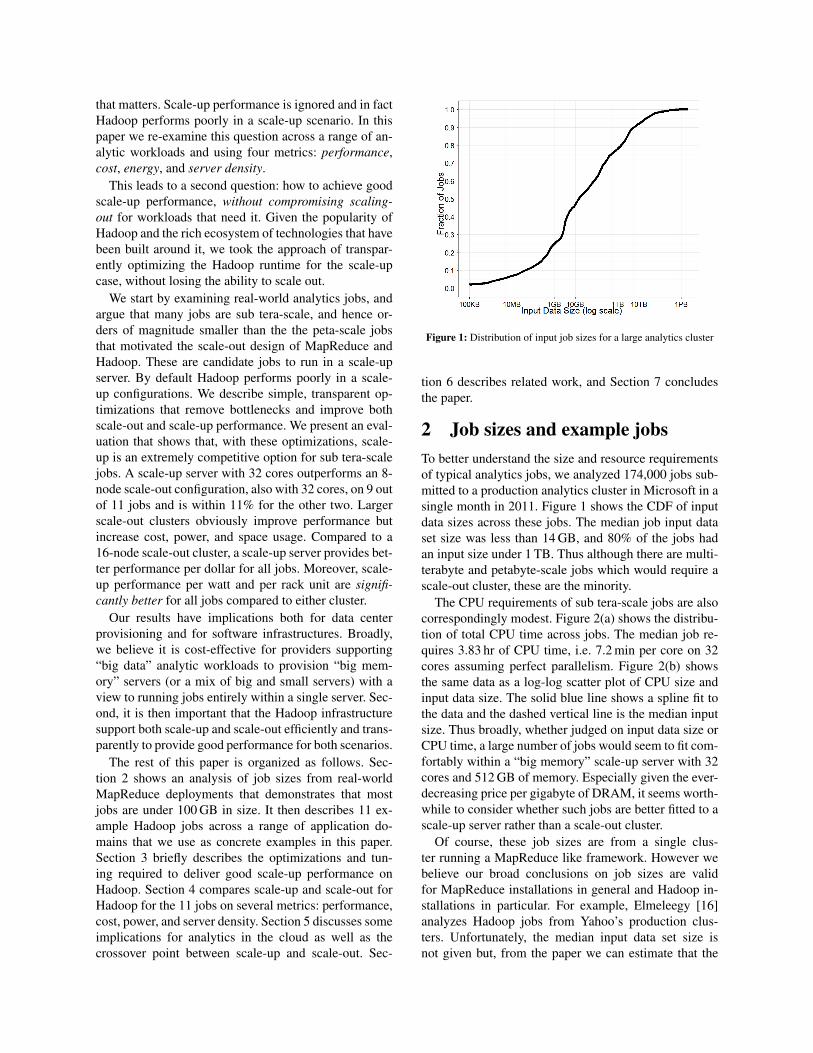
Figure 1: Distribution of input job sizes for a large analytics cluster

tion 6 describes related work, and Section 7 concludesthe paper.

2 Job sizes and example jobsTo better understand the size and resource requirementsof typical analytics jobs, we analyzed 174,000 jobs sub-mitted to a production analytics cluster in Microsoft in asingle month in 2011. Figure 1 shows the CDF of inputdata sizes across these jobs. The median job input dataset size was less than 14 GB, and 80% of the jobs hadan input size under 1 TB. Thus although there are multi-terabyte and petabyte-scale jobs which would require ascale-out cluster, these are the minority.

The CPU requirements of sub tera-scale jobs are alsocorrespondingly modest. Figure 2(a) shows the distribu-tion of total CPU time across jobs. The median job re-quires 3.83 hr of CPU time, i.e. 7.2 min per core on 32cores assuming perfect parallelism. Figure 2(b) showsthe same data as a log-log scatter plot of CPU size andinput data size. The solid blue line shows a spline fit tothe data and the dashed vertical line is the median inputsize. Thus broadly, whether judged on input data size orCPU time, a large number of jobs would seem to fit com-fortably within a “big memory” scale-up server with 32cores and 512 GB of memory. Especially given the ever-decreasing price per gigabyte of DRAM, it seems worth-while to consider whether such jobs are better fitted to ascale-up server rather than a scale-out cluster.

Of course, these job sizes are from a single clus-ter running a MapReduce like framework. However webelieve our broad conclusions on job sizes are validfor MapReduce installations in general and Hadoop in-stallations in particular. For example, Elmeleegy [16]analyzes Hadoop jobs from Yahoo’s production clus-ters. Unfortunately, the median input data set size isnot given but, from the paper we can estimate that the

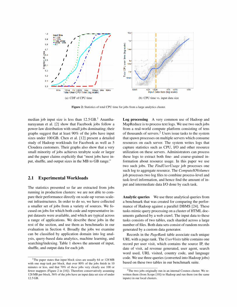
(a) CDF of CPU time (b) CPU time vs. input data size

Figure 2: Statistics of total CPU time for jobs from a large analytics cluster.

median job input size is less than 12.5 GB.1 Anantha-narayanan et al. [2] show that Facebook jobs follow apower-law distribution with small jobs dominating; theirgraphs suggest that at least 90% of the jobs have inputsizes under 100 GB. Chen et al. [12] present a detailedstudy of Hadoop workloads for Facebook as well as 5Cloudera customers. Their graphs also show that a verysmall minority of jobs achieves terabyte scale or largerand the paper claims explicitly that “most jobs have in-put, shuffle, and output sizes in the MB to GB range.”

2.1 Experimental Workloads

The statistics presented so far are extracted from jobsrunning in production clusters: we are not able to com-pare their performance directly on scale-up versus scale-out infrastructures. In order to do so, we have collecteda smaller set of jobs from a variety of sources. We fo-cused on jobs for which both code and representative in-put datasets were available, and which are typical acrossa range of applications. We describe these jobs in therest of the section, and use them as benchmarks in ourevaluation in Section 4. Broadly the jobs we examinecan be classified by application domain into log anal-ysis, query-based data analytics, machine learning, andsearching/indexing. Table 1 shows the amount of input,shuffle, and output data for each job.

1The paper states that input block sizes are usually 64 or 128 MBwith one map task per block, that over 80% of the jobs finish in 10minutes or less, and that 70% of these jobs very clearly use 100 orfewer mappers (Figure 2 in [16]). Therefore conservatively assuming128 MB per block, 56% of the jobs have an input data set size of under12.5 GB.

Log processing A very common use of Hadoop andMapReduce is to process text logs. We use two such jobsfrom a real-world compute platform consisting of tensof thousands of servers.2 Users issue tasks to the systemthat spawn processes on multiple servers which consumeresources on each server. The system writes logs thatcapture statistics such as CPU, I/O and other resourceutilization on these servers. Administrators can processthese logs to extract both fine- and coarse-grained in-formation about resource usage. In this paper we usetwo such jobs. The FindUserUsage job processes onesuch log to aggregate resource. The ComputeIOVolumesjob processes two log files to combine process-level andtask-level information, and hence find the amount of in-put and intermediate data I/O done by each task.

Analytic queries We use three analytical queries froma benchmark that was created for comparing the perfor-mance of Hadoop against a parallel DBMS [24]. Thesetasks mimic query processing on a cluster of HTML doc-uments gathered by a web crawl. The input data to thesetasks consists of two tables, each sharded across a largenumber of files. Both data sets consist of random recordsgenerated by a custom data generator.

Records in the PageRank table associate each uniqueURL with a page rank. The UserVisits table contains onerecord per user visit, which contains the source IP, thedate of visit, ad revenue generated, user agent, searchword used, URL visited, country code, and languagecode. We use three queries (converted into Hadoop jobs)based on these two tables in our benchmark suite.

2The two jobs originally run in an internal Cosmos cluster. We re-written them (from Scope [10]) to Hadoop and run them (on the sameinputs) in our local clusters.

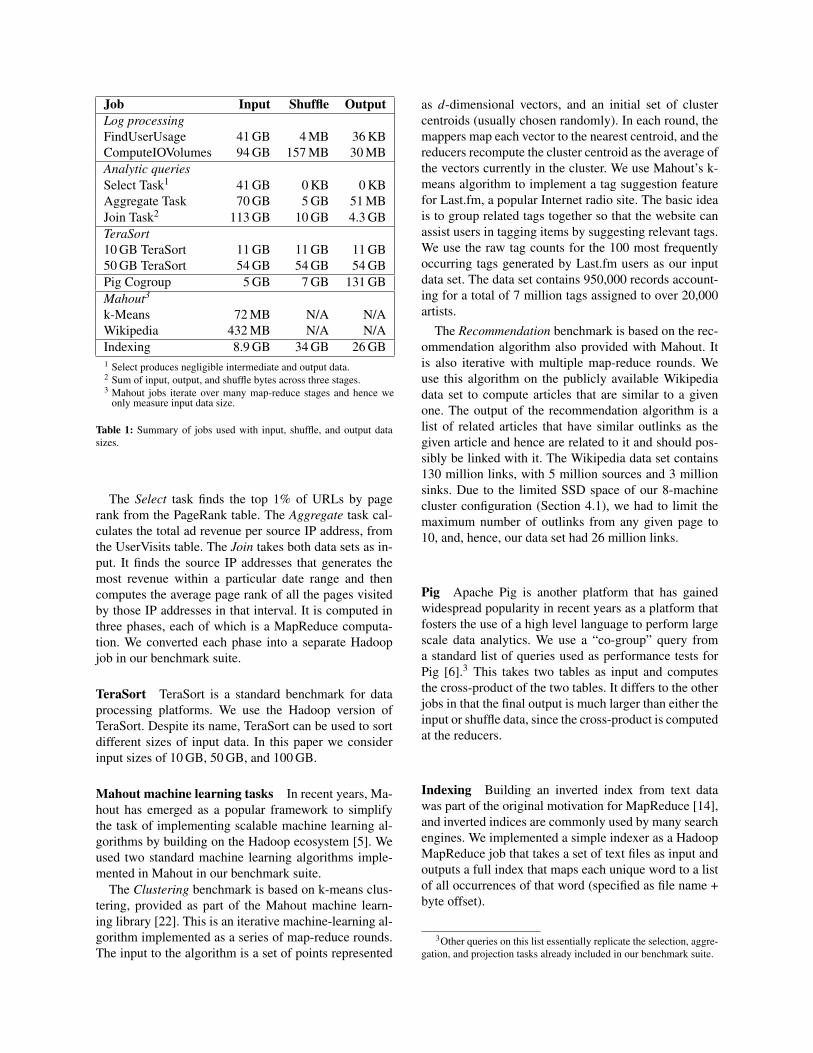
Job Input Shuffle OutputLog processingFindUserUsage 41 GB 4 MB 36 KBComputeIOVolumes 94 GB 157 MB 30 MBAnalytic queriesSelect Task1 41 GB 0 KB 0 KBAggregate Task 70 GB 5 GB 51 MBJoin Task2 113 GB 10 GB 4.3 GBTeraSort10 GB TeraSort 11 GB 11 GB 11 GB50 GB TeraSort 54 GB 54 GB 54 GBPig Cogroup 5 GB 7 GB 131 GBMahout3

k-Means 72 MB N/A N/AWikipedia 432 MB N/A N/AIndexing 8.9 GB 34 GB 26 GB1 Select produces negligible intermediate and output data.2 Sum of input, output, and shuffle bytes across three stages.3 Mahout jobs iterate over many map-reduce stages and hence we

only measure input data size.

Table 1: Summary of jobs used with input, shuffle, and output datasizes.

The Select task finds the top 1% of URLs by pagerank from the PageRank table. The Aggregate task cal-culates the total ad revenue per source IP address, fromthe UserVisits table. The Join takes both data sets as in-put. It finds the source IP addresses that generates themost revenue within a particular date range and thencomputes the average page rank of all the pages visitedby those IP addresses in that interval. It is computed inthree phases, each of which is a MapReduce computa-tion. We converted each phase into a separate Hadoopjob in our benchmark suite.

TeraSort TeraSort is a standard benchmark for dataprocessing platforms. We use the Hadoop version ofTeraSort. Despite its name, TeraSort can be used to sortdifferent sizes of input data. In this paper we considerinput sizes of 10 GB, 50 GB, and 100 GB.

Mahout machine learning tasks In recent years, Ma-hout has emerged as a popular framework to simplifythe task of implementing scalable machine learning al-gorithms by building on the Hadoop ecosystem [5]. Weused two standard machine learning algorithms imple-mented in Mahout in our benchmark suite.

The Clustering benchmark is based on k-means clus-tering, provided as part of the Mahout machine learn-ing library [22]. This is an iterative machine-learning al-gorithm implemented as a series of map-reduce rounds.The input to the algorithm is a set of points represented

as d-dimensional vectors, and an initial set of clustercentroids (usually chosen randomly). In each round, themappers map each vector to the nearest centroid, and thereducers recompute the cluster centroid as the average ofthe vectors currently in the cluster. We use Mahout’s k-means algorithm to implement a tag suggestion featurefor Last.fm, a popular Internet radio site. The basic ideais to group related tags together so that the website canassist users in tagging items by suggesting relevant tags.We use the raw tag counts for the 100 most frequentlyoccurring tags generated by Last.fm users as our inputdata set. The data set contains 950,000 records account-ing for a total of 7 million tags assigned to over 20,000artists.

The Recommendation benchmark is based on the rec-ommendation algorithm also provided with Mahout. Itis also iterative with multiple map-reduce rounds. Weuse this algorithm on the publicly available Wikipediadata set to compute articles that are similar to a givenone. The output of the recommendation algorithm is alist of related articles that have similar outlinks as thegiven article and hence are related to it and should pos-sibly be linked with it. The Wikipedia data set contains130 million links, with 5 million sources and 3 millionsinks. Due to the limited SSD space of our 8-machinecluster configuration (Section 4.1), we had to limit themaximum number of outlinks from any given page to10, and, hence, our data set had 26 million links.

Pig Apache Pig is another platform that has gainedwidespread popularity in recent years as a platform thatfosters the use of a high level language to perform largescale data analytics. We use a “co-group” query froma standard list of queries used as performance tests forPig [6].3 This takes two tables as input and computesthe cross-product of the two tables. It differs to the otherjobs in that the final output is much larger than either theinput or shuffle data, since the cross-product is computedat the reducers.

Indexing Building an inverted index from text datawas part of the original motivation for MapReduce [14],and inverted indices are commonly used by many searchengines. We implemented a simple indexer as a HadoopMapReduce job that takes a set of text files as input andoutputs a full index that maps each unique word to a listof all occurrences of that word (specified as file name +byte offset).

3Other queries on this list essentially replicate the selection, aggre-gation, and projection tasks already included in our benchmark suite.

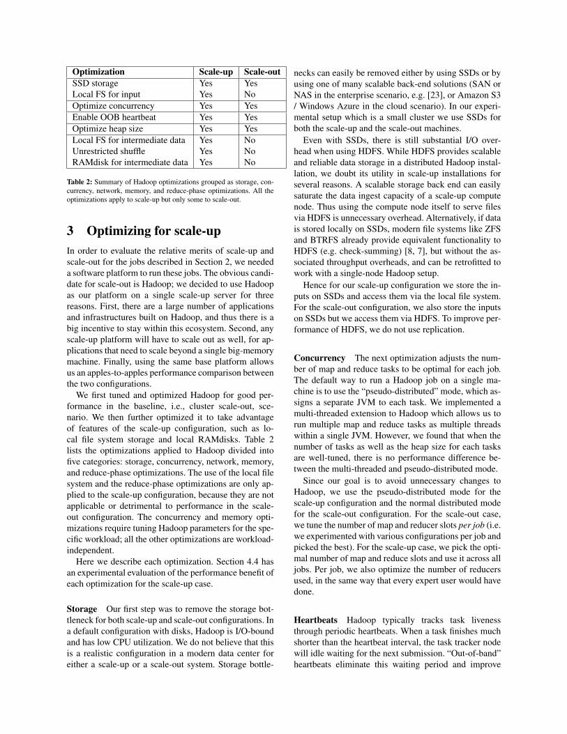
Optimization Scale-up Scale-outSSD storage Yes YesLocal FS for input Yes NoOptimize concurrency Yes YesEnable OOB heartbeat Yes YesOptimize heap size Yes YesLocal FS for intermediate data Yes NoUnrestricted shuffle Yes NoRAMdisk for intermediate data Yes No

Table 2: Summary of Hadoop optimizations grouped as storage, con-currency, network, memory, and reduce-phase optimizations. All theoptimizations apply to scale-up but only some to scale-out.

3 Optimizing for scale-upIn order to evaluate the relative merits of scale-up andscale-out for the jobs described in Section 2, we neededa software platform to run these jobs. The obvious candi-date for scale-out is Hadoop; we decided to use Hadoopas our platform on a single scale-up server for threereasons. First, there are a large number of applicationsand infrastructures built on Hadoop, and thus there is abig incentive to stay within this ecosystem. Second, anyscale-up platform will have to scale out as well, for ap-plications that need to scale beyond a single big-memorymachine. Finally, using the same base platform allowsus an apples-to-apples performance comparison betweenthe two configurations.

We first tuned and optimized Hadoop for good per-formance in the baseline, i.e., cluster scale-out, sce-nario. We then further optimized it to take advantageof features of the scale-up configuration, such as lo-cal file system storage and local RAMdisks. Table 2lists the optimizations applied to Hadoop divided intofive categories: storage, concurrency, network, memory,and reduce-phase optimizations. The use of the local filesystem and the reduce-phase optimizations are only ap-plied to the scale-up configuration, because they are notapplicable or detrimental to performance in the scale-out configuration. The concurrency and memory opti-mizations require tuning Hadoop parameters for the spe-cific workload; all the other optimizations are workload-independent.

Here we describe each optimization. Section 4.4 hasan experimental evaluation of the performance benefit ofeach optimization for the scale-up case.

Storage Our first step was to remove the storage bot-tleneck for both scale-up and scale-out configurations. Ina default configuration with disks, Hadoop is I/O-boundand has low CPU utilization. We do not believe that thisis a realistic configuration in a modern data center foreither a scale-up or a scale-out system. Storage bottle-

necks can easily be removed either by using SSDs or byusing one of many scalable back-end solutions (SAN orNAS in the enterprise scenario, e.g. [23], or Amazon S3/ Windows Azure in the cloud scenario). In our experi-mental setup which is a small cluster we use SSDs forboth the scale-up and the scale-out machines.

Even with SSDs, there is still substantial I/O over-head when using HDFS. While HDFS provides scalableand reliable data storage in a distributed Hadoop instal-lation, we doubt its utility in scale-up installations forseveral reasons. A scalable storage back end can easilysaturate the data ingest capacity of a scale-up computenode. Thus using the compute node itself to serve filesvia HDFS is unnecessary overhead. Alternatively, if datais stored locally on SSDs, modern file systems like ZFSand BTRFS already provide equivalent functionality toHDFS (e.g. check-summing) [8, 7], but without the as-sociated throughput overheads, and can be retrofitted towork with a single-node Hadoop setup.

Hence for our scale-up configuration we store the in-puts on SSDs and access them via the local file system.For the scale-out configuration, we also store the inputson SSDs but we access them via HDFS. To improve per-formance of HDFS, we do not use replication.

Concurrency The next optimization adjusts the num-ber of map and reduce tasks to be optimal for each job.The default way to run a Hadoop job on a single ma-chine is to use the “pseudo-distributed” mode, which as-signs a separate JVM to each task. We implemented amulti-threaded extension to Hadoop which allows us torun multiple map and reduce tasks as multiple threadswithin a single JVM. However, we found that when thenumber of tasks as well as the heap size for each tasksare well-tuned, there is no performance difference be-tween the multi-threaded and pseudo-distributed mode.

Since our goal is to avoid unnecessary changes toHadoop, we use the pseudo-distributed mode for thescale-up configuration and the normal distributed modefor the scale-out configuration. For the scale-out case,we tune the number of map and reducer slots per job (i.e.we experimented with various configurations per job andpicked the best). For the scale-up case, we pick the opti-mal number of map and reduce slots and use it across alljobs. Per job, we also optimize the number of reducersused, in the same way that every expert user would havedone.

Heartbeats Hadoop typically tracks task livenessthrough periodic heartbeats. When a task finishes muchshorter than the heartbeat interval, the task tracker nodewill idle waiting for the next submission. “Out-of-band”heartbeats eliminate this waiting period and improve

performance [13]. We enable them for both scale-up andscale-out configurations.

Heap size By default each Hadoop map and reducetask is run in a JVM with a 200 MB heap within whichthey allocate buffers for in-memory data. When thebuffers are full, data is spilled to storage, adding over-heads. We note that 200 MB per task leaves substan-tial amounts of memory unused on modern servers. Byincreasing the heap size for each JVM (and hence theworking memory for each task), we improve perfor-mance. However too large a heap size causes garbagecollection overheads, and wastes memory that could beused for other purposes (such as a RAMdisk). For thescale-out configurations, we found the optimal heap sizefor each job through trial and error. For the scale-up con-figuration we set a heap size of 4 GB per mapper/reducertask (where the maximum number of tasks is set to thenumber of processors) for all jobs.

Shuffle optimizations The next three optimizationsspeed up the shuffle (transferring data from mappersto reducers) on the scale-up configuration: they do notapply to scale-out configurations. First, we modifiedHadoop so that shuffle data is transferred by writing andreading the local file system; the default is for reducersto copy the data from the mappers via http. However, wefound that this still leads to underutilized storage band-width during the shuffle phase for our scale-up config-uration, due to a restriction on the number of concur-rent connections that is allowed. In a cluster, this is areasonable throttling scheme to avoid a single node get-ting overloaded by copy requests. However it is unneces-sary in a scale-up configuration with a fast local file sys-tem. Removing this limit substantially improves shuffleperformance. Finally, we observed that the scale-up ma-chine has substantial excess memory after configuringfor optimal concurrency level and heap size. We use thisexcess memory as a RAMdisk to store intermediate datarather than using an SSD or disk based file system.

4 EvaluationIn this section, we will use the benchmarks and MapRe-duce jobs we described in Section 2 to perform an in-depth analysis of the performance of scale-up and scale-out Hadoop.

To understand the pros and cons of scaling up as op-posed to scaling out, one needs to compare optimizedimplementations of both architectures side by side usingseveral metrics (such as performance, performance/unitcost, and performance/unit energy) under a wide rangeof benchmarks. In this section we first describe our ex-perimental setup. We then compare scale-up and scale-

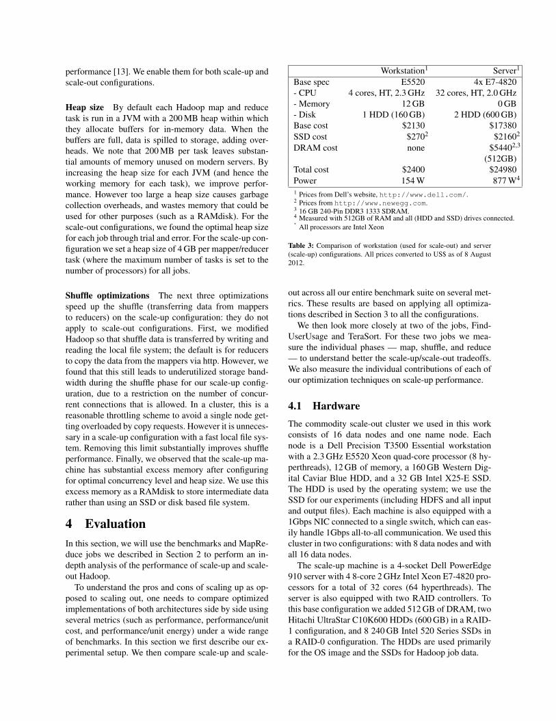
Workstation1 Server1

Base spec E5520 4x E7-4820- CPU 4 cores, HT, 2.3 GHz 32 cores, HT, 2.0 GHz- Memory 12 GB 0 GB- Disk 1 HDD (160 GB) 2 HDD (600 GB)Base cost $2130 $17380SSD cost $2702 $21602

DRAM cost none $54402,3

(512GB)Total cost $2400 $24980Power 154 W 877 W4

1 Prices from Dell’s website, http://www.dell.com/.2 Prices from http://www.newegg.com.3 16 GB 240-Pin DDR3 1333 SDRAM.4 Measured with 512GB of RAM and all (HDD and SSD) drives connected.∗

All processors are Intel Xeon

Table 3: Comparison of workstation (used for scale-out) and server(scale-up) configurations. All prices converted to US$ as of 8 August2012.

out across all our entire benchmark suite on several met-rics. These results are based on applying all optimiza-tions described in Section 3 to all the configurations.

We then look more closely at two of the jobs, Find-UserUsage and TeraSort. For these two jobs we mea-sure the individual phases — map, shuffle, and reduce— to understand better the scale-up/scale-out tradeoffs.We also measure the individual contributions of each ofour optimization techniques on scale-up performance.

4.1 HardwareThe commodity scale-out cluster we used in this workconsists of 16 data nodes and one name node. Eachnode is a Dell Precision T3500 Essential workstationwith a 2.3 GHz E5520 Xeon quad-core processor (8 hy-perthreads), 12 GB of memory, a 160 GB Western Dig-ital Caviar Blue HDD, and a 32 GB Intel X25-E SSD.The HDD is used by the operating system; we use theSSD for our experiments (including HDFS and all inputand output files). Each machine is also equipped with a1Gbps NIC connected to a single switch, which can eas-ily handle 1Gbps all-to-all communication. We used thiscluster in two configurations: with 8 data nodes and withall 16 data nodes.

The scale-up machine is a 4-socket Dell PowerEdge910 server with 4 8-core 2 GHz Intel Xeon E7-4820 pro-cessors for a total of 32 cores (64 hyperthreads). Theserver is also equipped with two RAID controllers. Tothis base configuration we added 512 GB of DRAM, twoHitachi UltraStar C10K600 HDDs (600 GB) in a RAID-1 configuration, and 8 240 GB Intel 520 Series SSDs ina RAID-0 configuration. The HDDs are used primarilyfor the OS image and the SSDs for Hadoop job data.

0

0.2

0.4

0.6

0.8

1

1.2

1.4

1.6

1.8

2

Scale-out (16) Scale-out (8)

No

rmal

ize

d p

erf

orm

ance

pe

r $

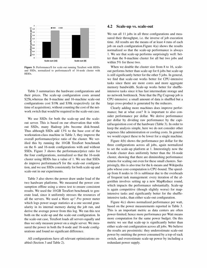
HDD SSD

Figure 3: Performance/$ for scale-out running TeraSort with HDDsand SSDs, normalized to performance/$ of 16-node cluster withHDDs.

Table 3 summarizes the hardware configurations andtheir prices. The scale-up configuration costs around$25k,whereas the 8-machine and 16-machine scale-outconfigurations cost $19k and $38k respectively (at thetime of acquisition), without counting the cost of the net-work switch that would be required in the scale-out case.

We use SSDs for both the scale-up and the scale-out server. This is based on our observation that with-out SSDs, many Hadoop jobs become disk-bound.Thus although SSDs add 13% to the base cost of theworkstation-class machine in Table 3, they improve theoverall performance/price ratio of the cluster. We ver-ified this by running the 10 GB TeraSort benchmarkon the 8- and 16-node configurations with and withoutSSDs. Figure 3 shows the performance/price ratio forthe four configurations, normalized so that the 16-nodecluster using HDDs has a value of 1. We see that SSDsdo improve performance/$ for the scale-out configura-tion, and we use SSDs consistently for both scale-up andscale-out in our experiments.

Table 3 also shows the power draw under load of thetwo hardware platforms. We measured the power con-sumption offline using a stress test to ensure consistentresults. We used the 10 GB TeraSort benchmark to gen-erate load, since it uniformly stresses the resources ofall the servers. We used a Watts up? Pro power meterwhich logs power usage statistics at a one second gran-ularity in its internal memory during the job run, andderive the average power from this log. We ran this testboth on the scale-up and the scale-out configuration. Inthe scale-out case, TeraSort loads all servers equally andthus we only measure power on a single server. We mea-sured the power in both the 8-node and 16-node config-urations and found no significant difference.

All configurations have all relevant optimizations en-abled (Section 3 and Table 2).

4.2 Scale-up vs. scale-out

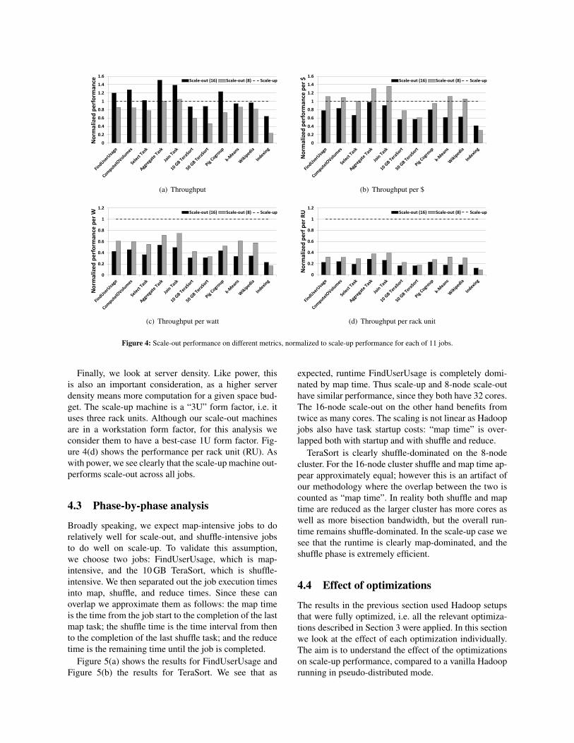
We ran all 11 jobs in all three configurations and mea-sured their throughput, i.e. the inverse of job executiontime. All results are the means of at least 4 runs of eachjob on each configuration.Figure 4(a) shows the resultsnormalized so that the scale-up performance is always1. We see that scale-up performs surprisingly well: bet-ter than the 8-machine cluster for all but two jobs andwithin 5% for those two.

When we double the cluster size from 8 to 16, scale-out performs better than scale-up for 6 jobs but scale-upis still significantly better for the other 5 jobs. In general,we find that scale-out works better for CPU-intensivetasks since there are more cores and more aggregatememory bandwidth. Scale-up works better for shuffle-intensive tasks since it has fast intermediate storage andno network bottleneck. Note that the Pig Cogroup job isCPU-intensive: a small amount of data is shuffled but alarge cross-product is generated by the reducers.

Clearly adding more machines does improve perfor-mance; but at what cost? It is important to also con-sider performance per dollar. We derive performanceper dollar by dividing raw performance by the capi-tal/acquisition cost of the hardware (Table 3). In order tokeep the analysis simple, here we do not consider otherexpenses like administration or cooling costs. In generalwe would expect these to be lower for a single machine.

Figure 4(b) shows the performance per dollar for thethree configurations across all jobs, again normalizedto set the scale-up platform at 1. Interestingly now the8-node cluster does uniformly better than the 16-nodecluster, showing that there are diminishing performancereturns for scaling out even for these small clusters. Sur-prisingly, this is also true for the k-means and Wikipediajobs whose core-computation is CPU-bound. The speed-up from 8 nodes to 16 is sublinear due to the overheadsof frequent task management: every iteration of the al-gorithm involves setting up a new MapReduce round,which impacts the performance substantially. Scale-upis again competitive (though slightly worse) for map-intensive tasks and significantly better for the shuffle-intensive tasks, than either scale-out configuration.

Figure 4(c) shows normalized performance per watt,based on the power measurements reported in Table 3.This is an important metric as data centers are oftenpower-limited; hence more performance per Watt meansmore computation for the same power budget. On thismetric we see that scale-up is significantly better thaneither scale-out configuration across all jobs. We believethe results are pessimistic: they underestimate scale-outpower by omitting the power consumed by a top-of-rackswitch, and overestimate scale-up power by including aredundant power supply.

0

0.2

0.4

0.6

0.8

1

1.2

1.4

1.6

No

rmal

ize

d p

erf

orm

ance

Scale-out (16) Scale-out (8) Scale-up

(a) Throughput

0

0.2

0.4

0.6

0.8

1

1.2

1.4

1.6

No

rmal

ize

d p

erf

orm

ance

pe

r $

Scale-out (16) Scale-out (8) Scale-up

(b) Throughput per $

0

0.2

0.4

0.6

0.8

1

1.2

No

rmal

ize

d p

erf

orm

ance

pe

r W

Scale-out (16) Scale-out (8) Scale-up

(c) Throughput per watt

0

0.2

0.4

0.6

0.8

1

1.2

No

rmal

ize

d p

erf

pe

r R

U

Scale-out (16) Scale-out (8) Scale-up

(d) Throughput per rack unit

Figure 4: Scale-out performance on different metrics, normalized to scale-up performance for each of 11 jobs.

Finally, we look at server density. Like power, thisis also an important consideration, as a higher serverdensity means more computation for a given space bud-get. The scale-up machine is a “3U” form factor, i.e. ituses three rack units. Although our scale-out machinesare in a workstation form factor, for this analysis weconsider them to have a best-case 1U form factor. Fig-ure 4(d) shows the performance per rack unit (RU). Aswith power, we see clearly that the scale-up machine out-performs scale-out across all jobs.

4.3 Phase-by-phase analysis

Broadly speaking, we expect map-intensive jobs to dorelatively well for scale-out, and shuffle-intensive jobsto do well on scale-up. To validate this assumption,we choose two jobs: FindUserUsage, which is map-intensive, and the 10 GB TeraSort, which is shuffle-intensive. We then separated out the job execution timesinto map, shuffle, and reduce times. Since these canoverlap we approximate them as follows: the map timeis the time from the job start to the completion of the lastmap task; the shuffle time is the time interval from thento the completion of the last shuffle task; and the reducetime is the remaining time until the job is completed.

Figure 5(a) shows the results for FindUserUsage andFigure 5(b) the results for TeraSort. We see that as

expected, runtime FindUserUsage is completely domi-nated by map time. Thus scale-up and 8-node scale-outhave similar performance, since they both have 32 cores.The 16-node scale-out on the other hand benefits fromtwice as many cores. The scaling is not linear as Hadoopjobs also have task startup costs: “map time” is over-lapped both with startup and with shuffle and reduce.

TeraSort is clearly shuffle-dominated on the 8-nodecluster. For the 16-node cluster shuffle and map time ap-pear approximately equal; however this is an artifact ofour methodology where the overlap between the two iscounted as “map time”. In reality both shuffle and maptime are reduced as the larger cluster has more cores aswell as more bisection bandwidth, but the overall run-time remains shuffle-dominated. In the scale-up case wesee that the runtime is clearly map-dominated, and theshuffle phase is extremely efficient.

4.4 Effect of optimizations

The results in the previous section used Hadoop setupsthat were fully optimized, i.e. all the relevant optimiza-tions described in Section 3 were applied. In this sectionwe look at the effect of each optimization individually.The aim is to understand the effect of the optimizationson scale-up performance, compared to a vanilla Hadooprunning in pseudo-distributed mode.

50 57

38

4

3

4

2

2

4

0

10

20

30

40

50

60

70

Scale-up Scale-out (8) Scale-out (16)

Job

ru

nti

me

(Se

con

ds)

Reduce Time

Shuffle Time

Map time

(a) FindUserUsage

42 40 33

4

67

27 10

18

8

0

20

40

60

80

100

120

140

Scale-up Scale-out (8) Scale-out (16)

Job

ru

ntm

e (

Seco

nd

s)

Reduce Time

Shuffle Time

Map Time

(b) 10 GB TeraSort

Figure 5: Runtime for different phases with FindUserUsage and10 GB TeraSort

We examine two jobs from our benchmark suite. Find-UserUsage is map-intensive with little intermediate dataand a small reduce phase. We use it to measure all op-timizations except those that improve the shuffle phase,since the shuffle phase in FindUserUsage is very small.TeraSort is memory- and shuffle- intensive. Thus we useit to measure the effect of the memory and shuffle-phaseoptimizations. In all cases we use the scale-up server de-scribed previously.

Figure 6(a) shows the effect on FindUserUsage’s ex-ecution time of successively moving from disk-basedHDFS to an SSD-based local file system; of optimiz-ing the number of mappers and reducers; of removingout-of-band heartbeats; and of optimizing the heap size.Each has a significant impact, with a total performanceimprovement of 4x.

Figure 6(b) shows the effect on execution time of10 GB TeraSort starting from a baseline where the stor-age, concurrency, and heartbeat optimizations have al-ready been applied. The heap size optimization has a sig-nificant effect, as input and intermediate data buffers arespilled less frequently to the file system. Moving to thefile system based rather than http based shuffle and un-throttling the shuffle has an even bigger effect. Finally,using a RAMdisk for that intermediate data improves

255

157

121

82 64

0

50

100

150

200

250

300

Baseline SSD storage Concurrency Heartbeat Heap size

Exe

cuti

on

tim

e (

s)

(a) Effect of input storage, concurrency, heartbeat, and heap optimiza-tions on FindUserUsage

414

221

100

63

0

50

100

150

200

250

300

350

400

450

SSD storage +concurrency +

heartbeat

Heap size Local FS + unrestrictedshuffle

RAMDisk

Exe

cuti

on

tim

e (

s)

(b) Effect of memory and shuffle optimizations on 10 GB TeraSort

Figure 6: Effect of different optimizations on FindUserUsage and10 GB TeraSort

performance even further. For TeraSort, heap size opti-mization improves performance by 2x and shuffle-phaseoptimizations by almost 3.5x, for a total performanceimprovement of 7x.

5 DiscussionIn Section 4 we evaluated 11 read-world jobs to showthat scale-up is competitive on performance and perfor-mance/$, and superior on performance per watt and perrack unit. Here we consider implications for cloud com-puting, and discuss the limits of scale-up.

5.1 Scale up vs. scale-out in the cloudOur analysis so far was based on a private clusterand scale-up machine. As many analytic jobs includ-ing Hadoop jobs are now moving to the cloud, it isworth asking, how will our results apply in the cloudscenario? The key difference from a private cluster isthat in the cloud, a scalable storage back end, such as S3or Azure Storage, is likely to be used for input data (in-stead of HDFS), and the compute nodes, at least today,are unlikely to use SSD storage. Intermediate data willbe stored in memory or local disk.

0.43

0.72

0.60

0.50

0.00

0.20

0.40

0.60

0.80

1.00

Normalized Performance Normalized Performance / $

Scale-Out (8) Scale-Out (16)

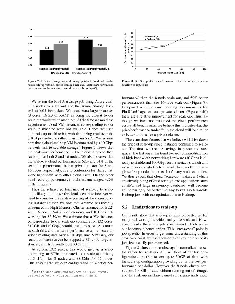
Figure 7: Relative throughput and throughput/$ of cloud and single-node scale-up with a scalable storage back-end. Results are normalizedwith respect to the scale-up throughput and throughput/$.

We re-ran the FindUserUsage job using Azure com-pute nodes to scale out and the Azure Storage backend to hold input data. We used extra-large instances(8 cores, 16 GB of RAM) as being the closest to ourscale-out workstation machines. At the time we ran theseexperiments, cloud VM instances corresponding to ourscale-up machine were not available. Hence we usedour scale-up machine but with data being read over the(10 Gbps) network rather than from SSD. (We assumehere that a cloud scale-up VM is connected by a 10 Gbpsnetwork link to scalable storage.) Figure 7 shows thatthe scale-out performance in the cloud is worse thanscale-up for both 8 and 16 nodes. We also observe thatthe scale-out cloud performance is 62% and 64% of thescale-out performance in our private cluster for 8 and16 nodes respectively, due to contention for shared net-work bandwidth with other cloud users. On the otherhand scale-up performance is almost unchanged (92%of the original).

Thus the relative performance of scale-up to scale-out is likely to improve for cloud scenarios; however weneed to consider the relative pricing of the correspond-ing instances either. We note that Amazon has recentlyannounced its High-Memory Cluster Instance for EC24

with 16 cores, 244 GiB of memory, and 10 Gbps net-working for $3.50/hr. We estimate that a VM instancecorresponding to our scale-up configuration (32 cores,512 GB, and 10 Gbps) would cost at most twice as muchas such this, and the same performance as our scale-upserver reading data over a 10 Gbps link. Similarly, ourscale-out machines can be mapped to M1 extra-large in-stances, which currently cost $0.52/hr.

At current EC2 prices, this would give us a scale-up pricing of $7/hr, compared to a scale-out pricingof $4.16/hr for 8 nodes and $8.32/hr for 16 nodes.This gives us the scale-up configuration 38% better per-

4http://docs.aws.amazon.com/AWSEC2/latest/UserGuide/using_cluster_computing.html

0

0.1

0.2

0.3

0.4

0.5

0.6

0.7

0.8

0.9

1

0 20 40 60 80 100 120

Pe

rfo

rman

ce/$

re

lati

ve t

o

scal

e-u

p

TeraSort input size (GB)

Scale-out (8)

Scale-out (16)

Figure 8: TeraSort performance/$ normalized to that of scale-up as afunction of input size

formance/$ than the 8-node scale-out, and 50% betterperformance/$ than the 16-node scale-out (Figure 7).Compared with the corresponding measurements forFindUserUsage on our private cluster (Figure 4(b))these are a relative improvement for scale-up. Thus, al-though we have not evaluated the cloud performanceacross all benchmarks, we believe this indicates that theprice/performance tradeoffs in the cloud will be similaror better to those for a private cluster.

There are three factors that we believe will drive downthe price of scale-up cloud instances compared to scale-out. The first two are the savings in power and rackspace. The last one is the trend towards commoditizationof high-bandwidth networking hardware (40 Gbps is al-ready available and 100 Gbps on the horizon), which willmake it more cost-effective to add bandwidth to a sin-gle scale-up node than to each of many scale-out nodes.We thus expect that cloud “scale-up” instances (whichare already being offered for high-end applications suchas HPC and large in-memory databases) will becomean increasingly cost-effective way to run sub tera-scaleHadoop jobs with our optimizations to Hadoop.

5.2 Limitations to scale-up

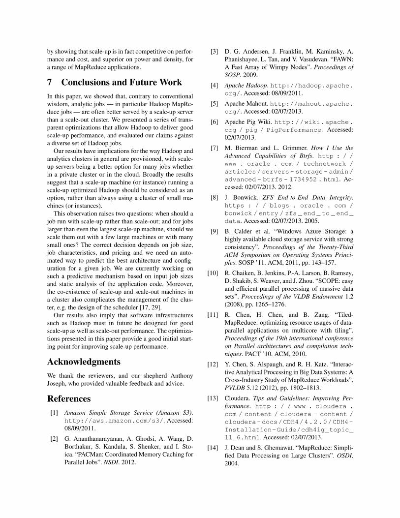
Our results show that scale-up is more cost-effective formany real-world jobs which today use scale-out. How-ever, clearly there is a job size beyond which scale-out becomes a better option. This “cross-over” point isjob-specific. In order to get some understanding of thiscrossover point, we use TeraSort as an example since itsjob size is easily parametrized.

Figure 8 shows the results, again normalized to setthe values for scale-up at 1. All three of our test con-figurations are able to sort up to 50 GB of data, withthe scale-up configuration providing by far the best per-formance per dollar. However the 8-node cluster can-not sort 100 GB of data without running out of storage,and the scale-up machine cannot sort significantly more

than 100 GB without running out of memory. At 100 GB,scale-up still provides the best performance/$, but the16-node cluster is close at 88% of scale-up.

These results tell us two things. First, even with“big memory”, the scale-up configuration can becomememory-bound for large jobs. However we expect thispoint to shift upwards as DRAM prices continue to falland multiple terabytes of DRAM per machine becomefeasible. Second, for TeraSort, scale-out is competitiveat around the 100 GB mark with current hardware.

More generally, while it is feasible to have a mix oflarge and small machines (and cloud providers alreadyprovide a mix of instance sizes), it is not desirable tomaintain two versions of each application. By making allour changes transparently “under the hood” of Hadoop,we allow the decision of scale-up versus scale-out to bemade transparently to the application.

6 Related WorkOne of the motivations for this work was the observationthat most analytic job sizes are well within the 512 GBthat is feasible on a standard “scale-up” server today. Wecollected information about job sizes internally, wherewe found median job sizes to be less than 14 GB, butour conclusions are also supported by studies on a rangeof real-world Hadoop installations including Yahoo [16],Facebook [2, 12], and Cloudera [12].

Piccolo [25] is an in-memory distributed key-valuestore, aimed at applications that need low-latency fine-grained random access to state. Resilient DistributedDatasets (RDDs) [33] similarly offer a distributed mem-ory like abstraction in the Spark system, but are aimedat task-parallel jobs, especially iterative machine learn-ing jobs such as the Mahout jobs considered in this pa-per. Both of these are “in-memory scale-out” solutions:they remove the disk I/O bottleneck by keeping data inmemory. However they still suffer from the network bot-tleneck of fetching remote data or shuffling data in aMapReduce computation. Our contribution is to showthat scale-up rather than scale-out is a competitive op-tion even for task-parallel jobs (both iterative and non-iterative) and can be done with transparent optimizationsthat maintain app-compatibility with Hadoop.

Phoenix [26, 32, 30], Metis [20], and Tiled-MapReduce [11] are in-memory multi-core (i.e. scale-up) optimized MapReduce libraries. They demonstratethat a carefully engineered MapReduce library can becompetitive with a shared-memory multi-threaded im-plementation. In this paper we make a similar observa-tion about multi-threaded vs. MapReduce in the Hadoopcontext. However our distinct contribution is that weprovide good scale-up performance transparently forHadoop jobs; and we evaluate the tradeoffs of scale-up

vs. scale-out by looking at job sizes as well as perfor-mance, dollar cost, power, and server density.

GraphChi [18] also advocates processing big data ina single machine. They focus on graph computations,and argue that, by carefully scheduling disk operationsand computations, even commodity machines can pro-cess very large graphs.

Michael et al. [21] studied the problem of scale-up vsscale-out for an interactive application (query process-ing in web search). They find scale-out to have a bet-ter performance per price ratio than scale-up. Observe,however, the differences in the context compared to ourwork (answering user queries versus data analytics re-spectively), and in the underlying hardware (IBM Blade-Center vs commodity PCs). They also find that runningscale-out in a box gives better performance than usingmulti-threading.

In previous work [28] we showed that certain machinelearning algorithms do not fit well within a MapReduceframework and hence both accuracy and performancewere improved by running them as shared-memory pro-grams on a single scale-up server. However this ap-proach means that each algorithm be implemented oncefor a multi-threaded shared-memory model and again forMapReduce if scale-out is also desired. Hence in thispaper we demonstrate how scale-up can be done trans-parently for Hadoop applications without sacrificing thepotential for scale-out and without a custom shared-memory implementation. We believe that while custommulti-threaded implementations might be necessary forcertain algorithms, they are expensive in terms of hu-man effort and notoriously hard to implement correctly.Transparent scale-up using Hadoop is applicable for amuch broader range of applications which are alreadywritten to use Hadoop MapReduce.

The tradeoff between low-power cores and a smallernumber of server-grade cores was extensively studiedby Reddi et al. [27] in the context of web search, andby Andersen et al. [3] in the context of a key-valuestorage system. Those works study the problem in dif-ferent context and reach opposite conclusions. Ander-sen et al. [3] argues that scale-out is more cost andpower effective than scale-up (for key-value storage sys-tems). Reddi et al. [27] reach similar conclusions tous (although for a different context). Similarly, recentwork [19] shows that for TPC-H queries, a cluster oflow-power Atom processors is not cost-effective com-pared to a traditional Xeon processor. In general, thescale-up versus scale-out tradeoff is well-known in theparallel database community [15]. A key observationis that the correct choice of scale-up versus scale-outis workload-specific. However in the MapReduce worldthe conventional wisdom is that scale-out is the only in-teresting option. We challenge this conventional wisdom

by showing that scale-up is in fact competitive on perfor-mance and cost, and superior on power and density, fora range of MapReduce applications.

7 Conclusions and Future WorkIn this paper, we showed that, contrary to conventionalwisdom, analytic jobs — in particular Hadoop MapRe-duce jobs — are often better served by a scale-up serverthan a scale-out cluster. We presented a series of trans-parent optimizations that allow Hadoop to deliver goodscale-up performance, and evaluated our claims againsta diverse set of Hadoop jobs.

Our results have implications for the way Hadoop andanalytics clusters in general are provisioned, with scale-up servers being a better option for many jobs whetherin a private cluster or in the cloud. Broadly the resultssuggest that a scale-up machine (or instance) running ascale-up optimized Hadoop should be considered as anoption, rather than always using a cluster of small ma-chines (or instances).

This observation raises two questions: when should ajob run with scale-up rather than scale-out; and for jobslarger than even the largest scale-up machine, should wescale them out with a few large machines or with manysmall ones? The correct decision depends on job size,job characteristics, and pricing and we need an auto-mated way to predict the best architecture and config-uration for a given job. We are currently working onsuch a predictive mechanism based on input job sizesand static analysis of the application code. Moreover,the co-existence of scale-up and scale-out machines ina cluster also complicates the management of the clus-ter, e.g. the design of the scheduler [17, 29].

Our results also imply that software infrastructuressuch as Hadoop must in future be designed for goodscale-up as well as scale-out performance. The optimiza-tions presented in this paper provide a good initial start-ing point for improving scale-up performance.

AcknowledgmentsWe thank the reviewers, and our shepherd AnthonyJoseph, who provided valuable feedback and advice.

References[1] Amazon Simple Storage Service (Amazon S3).

http://aws.amazon.com/s3/. Accessed:08/09/2011.

[2] G. Ananthanarayanan, A. Ghodsi, A. Wang, D.Borthakur, S. Kandula, S. Shenker, and I. Sto-ica. “PACMan: Coordinated Memory Caching forParallel Jobs”. NSDI. 2012.

[3] D. G. Andersen, J. Franklin, M. Kaminsky, A.Phanishayee, L. Tan, and V. Vasudevan. “FAWN:A Fast Array of Wimpy Nodes”. Proceedings ofSOSP. 2009.

[4] Apache Hadoop. http://hadoop.apache.org/. Accessed: 08/09/2011.

[5] Apache Mahout. http://mahout.apache.org/. Accessed: 02/07/2013.

[6] Apache Pig Wiki. http://wiki.apache.org / pig / PigPerformance. Accessed:02/07/2013.

[7] M. Bierman and L. Grimmer. How I Use theAdvanced Capabilities of Btrfs. http : / /www . oracle . com / technetwork /articles/servers- storage- admin/advanced - btrfs - 1734952 . html. Ac-cessed: 02/07/2013. 2012.

[8] J. Bonwick. ZFS End-to-End Data Integrity.https : / / blogs . oracle . com /bonwick / entry / zfs _ end _ to _ end _data. Accessed: 02/07/2013. 2005.

[9] B. Calder et al. “Windows Azure Storage: ahighly available cloud storage service with strongconsistency”. Proceedings of the Twenty-ThirdACM Symposium on Operating Systems Princi-ples. SOSP ’11. ACM, 2011, pp. 143–157.

[10] R. Chaiken, B. Jenkins, P.-A. Larson, B. Ramsey,D. Shakib, S. Weaver, and J. Zhou. “SCOPE: easyand efficient parallel processing of massive datasets”. Proceedings of the VLDB Endowment 1.2(2008), pp. 1265–1276.

[11] R. Chen, H. Chen, and B. Zang. “Tiled-MapReduce: optimizing resource usages of data-parallel applications on multicore with tiling”.Proceedings of the 19th international conferenceon Parallel architectures and compilation tech-niques. PACT ’10. ACM, 2010.

[12] Y. Chen, S. Alspaugh, and R. H. Katz. “Interac-tive Analytical Processing in Big Data Systems: ACross-Industry Study of MapReduce Workloads”.PVLDB 5.12 (2012), pp. 1802–1813.

[13] Cloudera. Tips and Guidelines: Improving Per-formance. http : / / www . cloudera .com / content / cloudera - content /cloudera-docs/CDH4/4.2.0/CDH4-Installation-Guide/cdh4ig_topic_11_6.html. Accessed: 02/07/2013.

[14] J. Dean and S. Ghemawat. “MapReduce: Simpli-fied Data Processing on Large Clusters”. OSDI.2004.

[15] D. DeWitt and J. Gray. “Parallel Database Sys-tems: The Future of High Performance DatabaseSystems”. Communications of the ACM 35.6(1992), pp. 85–98.

[16] K. Elmeleegy. “Piranha: Optimizing Short JobsIn Hadoop”. VLDB. 2013.

[17] B. Hindman, A. Konwinski, M. Zaharia, A. Gh-odsi, A. D. Joseph, R. Katz, S. Shenker, andI. Stoica. “Mesos: A Platform for Fine-GrainedResource Sharing in the Data Center”. Proceed-ings of the 8th USENIX Symposium on NetworkedSystems Design and Implementation. NSDI’11.USENIX, 2011.

[18] A. Kyrola, G. Blelloch, and C. Guestrin.“GraphChi: large-scale graph computation on justa PC”. Proceedings of the 10th USENIX con-ference on Operating Systems Design and Im-plementation. OSDI’12. USENIX Association,2012, pp. 31–46.

[19] W. Lang, J. M. Patel, and S. Shankar. “WimpyNode Clusters: What About Non-Wimpy Work-loads?” Workshop on Data Management on NewHardware (DaMon). 2010.

[20] Y. Mao, R. Morris, and F. Kaashoek. OptimizingMapReduce for Multicore Architectures. Tech.rep. MIT-CSAIL-TR-2010-020. MIT CSAIL,2010.

[21] M. Michael, J. E. Moreira, D. Shiloach, and R.W. Wisniewski. “Scale-up x Scale-out: A CaseStudy using Nutch/Lucene”. Proceedings of theIEEE International Symposium on Parallel andDistributed Processing. IPDPS’07. IEEE, 2007,pp. 1–8.

[22] S. Owen, R. Anil, T. Dunning, and E. Fried-man. Mahout in Action. Manning PublicationsCo., 2011.

[23] Panasas. Accelerating and Simplifying ApacheHadoop with Panasas ActiveStor. http : / /www . panasas . com / sites / default /files/uploads/docs/hadoop_wp_lr_1096.pdf. Accessed: 02/07/2013.

[24] A. Pavlo, E. Paulson, A. Rasin, D. J. Abadi, D. J.DeWitt, S. Madden, and M. Stonebraker. “A com-parison of approaches to large-scale data analy-sis”. SIGMOD ’09: Proceedings of the 35th SIG-

MOD international conference on Managementof data. ACM, 2009, pp. 165–178.

[25] R. Power and J. Li. “Piccolo: Building Fast,Distributed Programs with Partitioned Tables”.USENIX Symposium on Operating Systems De-sign and Implementation (OSDI). 2010.

[26] C. Ranger, R. Raghuraman, A. Penmetsa, G. R.Bradski, and C. Kozyrakis. “Evaluating MapRe-duce for Multi-core and Multiprocessor Sys-tems”. HPCA. 2007.

[27] V. J. Reddi, B. C. Lee, T. M. Chilimbi, and K.Vaid. “Web search using mobile cores: Quantify-ing and mitigating the price of efficiency”. Proc.37th International Symposium on Computer Ar-chitecture (37th ISCA’10). 2010, pp. 314–325.

[28] A. Rowstron, D. Narayanan, A. Donnelly, G.O’Shea, and A. Douglas. “Nobody ever got firedfor using Hadoop”. Workshop on Hot Topics inCloud Data Processing (HotCDP). 2012.

[29] M. Schwarzkopf, A. Konwinski, M. Abd-El-Malek, and J. Wilkes. “Omega: flexible, scal-able schedulers for large compute clusters”. Pro-ceedings of the 8th ACM European Conferenceon Computer Systems. EuroSys’13. ACM, 2013,pp. 351–364.

[30] J. Talbot, R. M. Yoo, and C. Kozyrakis.“Phoenix++: Modular MapReduce for Shared-Memory Systems”. Second InternationalWorkshop on MapReduce and its Applications(MAPREDUCE). 2011.

[31] Windows Azure Storage. http : / / www .microsoft . com / windowsazure /features/storage/. Accessed: 08/09/2011.

[32] R. M. Yoo, A. Romano, and C. Kozyrakis.“Phoenix Rebirth: Scalable MapReduce on aLarge-Scale Shared-Memory System”. IEEE In-ternational Symposium on Workload Characteri-zation (IISWC). 2009.

[33] M. Zaharia, M. Chowdhury, T. Das, A. Dave, J.Ma, M. McCauley, M. J. Franklin, S. Shenker,and I. Stoica. “Resilient Distributed Datasets:A Fault-Tolerant Abstraction for In-MemoryCluster Computing”. USENIX Symposium onNetworked Systems Design and Implementation(NSDI). 2012.