Scaling Environmental Processes in Heterogeneous Arid ... · Scaling Environmental Processes in Heterogeneous Arid ... program entitled “Scaling Environmental Processes in Heterogeneous

Scaling Environmental Processes in Heterogeneous Arid Soils: Construction of Large Weighing Lysimeter Facility Karletta Chief Michael H. Young Brad F. Lyles John Healey Jeremy Koonce Eric Knight Elizabeth Johnson Jarai Mon Markus Berli Menoj Menon Gayle Dana

December 2009

Publication No. 41249 prepared by Division of Hydrologic Sciences Desert Research Institute, Nevada System of Higher Education

THIS PAGE INTENTIONALLY LEFT BLANK

iii

PREFACE The inability to upscale or downscale arid environmental processes influences

research areas of hydrology, biogeosciences, mathematical modeling, and global environmental change. Research facilities that span small (column) to larger (basin) scales are either rare or nonexistent. To address this issue, researchers from Nevada’s universities constructed a weighing lysimeter facility in Boulder City, NV, under the NSF-funded program entitled “Scaling Environmental Processes in Heterogeneous Arid Soils” or SEPHAS. Four stainless steel lysimeters (three installed to date) are weighed on separate scales, each with a live mass of approximately 28,000 kg with a resolution of roughly 72-408 g or 0.018-0.102 mm of water. Each lysimeter is equipped with dataloggers that can be accessed remotely so investigators can monitor individual sensors and weather systems as needed. This meso-scale facility is devoted to investigating the near-surface interactions of soil, water, biota, and atmospheric processes that affect desert environments similar to those found in the southwestern United States such as the Mojave Desert and will bridge existing eco-scale, laboratory, and micro-scale research efforts.

Three lysimeters are cylindrical (2.258 m inner diameter x 3 m height), and one is square (2 m length x 2 m width x 3 m height). Each contains 12 m3 of either repacked or intact desert soil and is instrumented with 152 sensors that include 17 different technologies measuring water content, matric potential, temperature, thermal properties, electrical conductivity, soil settlement, and erosion; sampling pore water; and obtaining soil and root imagery. Specifically, a relatively new technology called distributed temperature sensing system was installed to obtain horizontal temperature profiles at six depths and a continuous vertical temperature profile. Also, during packing, four conservative tracers were applied uniformly at four depths from 0.15 to 0.55 m. Solution samplers installed at seven depths from 0.50 to 2.9 m to collect soil solution during irrigation experiments. Native desert shrubs will be installed in two replicate lysimeters in the spring of 2010 and three horizontal (installed at depths from 0.60 to 1.50 m) and one vertical mini-rhizotron tubes will be used to examine rooting behavior and water balance in recently disturbed soil.

This report contains 7 chapters that describe the construction and installation of this unique facility. The lysimeters were designed to investigate: 1) landscape dynamics, restoration, and water balance; 2) carbon sequestration; and 3) characteristics of soil properties at different scales. Within these general categories, the following hypotheses were developed:

• disturbance of structured desert soils will alter near-surface soil water balance, rates of biogeochemical weathering, water flow, plant rooting, and thermal and water content profiles;

• an increase in water infiltration will result in an increase in both soil PCO2 and water content; while an increase in Ca availability will favor carbon sequestration through the precipitation of CaCO3; and

• effective soil hydraulic properties can be estimated using only moisture content and without complex numerical techniques; characterizing heterogeneity in soil hydraulic properties can be accomplished with fewer physical property measurements; and scale effects create discrepancies in the measurement of hydrologic variables.

iv


v

ACKNOWLEDGEMENTS Funding for this research was provided by the National Science Foundation EPSCoR

project EPS 0447416. The authors thank projector leader, Michael H. Young (Desert Reseach Institute-DRI) who managed the project with assistance from representatives of University of Nevada, Reno-UNR (Scott Tyler) and University of Nevada, Las Vegas-UNLV (Zhongbo Yu). We also thank 1) the steering committee which included Dale A. Devitt (UNLV), Paul S.J. Verburg (DRI), and the project leaders; 2) the external review panel consisting of Steve Evett (USDA-ARS), Robert Graham (University of California, Riverside), and Peter Wierenga (University of Arizona); and 3) the senior personnel in the soils focal area including Darko Koracin (DRI), John A. Arnone III (DRI), Clay Cooper (DRI), Dave Decker (DRI), Michael J. Nicholl (UNLV), Robert S. Nowak (UNR), Henry Sun (DRI), and Paul S.J. Verburg (DRI). These individuals contributed valuable input for the proposal, facility design, and research development.

The installation, and implementation of this research facility was made possible by the collaborative efforts of the Boulder City SEPHAS team, including Karletta Chief, John Healey, Elizabeth Johnson, Jeremy Koonce, Eric Knight, and Michael H. Young, as well as input received from many principal investigators, staff scientists, post-doctoral fellows, and students. Specifically, the authors would like to thank Markus Berli for the design and installation of surface alteration probes; Todd Caldwell for the initial heat dissipation unit (HDU) datalogger program and soil physical analysis; Karletta Chief for calibration of HDUs and time-domain reflectometers, soil characterization, soil hydraulic and physical analysis, and site management and; Dale Devitt for use of the rain simulator and assistance in obtaining a uniformity coefficient; Karen Gray for database development; Mark Hausner, Jeremy Koonce, and Menoj Menon for the design, construction, and calibration of the distributed temperature sensing system; John Healey for the design, construction, and implementation of instruments and tools needed to install the lysimeters; Elizabeth Johnson for instrument mapping, design, cataloging, and installation, re-vegetation of facility field plot, and data quality assurance; Eric Knight for the installation of the lysimeters and site management; Jeremy Koonce for obtaining baseline rhizotron tube scans; Brad Lyles for assistance in extensive datalogger programming, datalogger and instrument design, setup, and wiring, data quality assurance, and database development; Jarai Mon, Hongwei Liu, and Xiang Long for laboratory sorption studies and application of tracers; Menoj Menon and Paul S.J. Verburg for design and application of nitrate tracers; and Michael H. Young for overall project management, instrument design research and field direction, data quality assurance, and database development.

We acknowledge seed grant researchers (funded to generate data for proposals and papers) at DRI (Kumud Acharya, John A. Arnone III, Markus Berli, Richard Jasoni, Giles Marion, Daniel Obrist, Mark C. Stone, Paul S.J. Verburg, Michael H. Young, and Jianting Zhu); UNLV (James Cizdziel, Dale A. Devitt, Michael J. Nicholl, Adam Simon, and Zhongbo Yu); UNR (Glenn Miller, Robert S. Nowak, and Scott W. Tyler); College of Southern Nevada (Kaveh Zarrabi); and Lawrence Berkeley National Laboratory (Teamrat Ghezzehei). The SEPHAS funded post-doctoral fellows including Karletta Chief (DRI), Manoj Menon (UNR), and Jarai Mon (UNLV) and one doctoral student, Jeremy Koonce (UNLV), are also acknowledged. Finally, we thank the reviewers and their suggestions which made this report a stronger publication.

vi


vii

CONTENTS PREFACE....................................................................................................................................iii ACKNOWLEDGEMENTS.......................................................................................................... v LIST OF FIGURES ..................................................................................................................... ix LIST OF TABLES.....................................................................................................................xiii ACRONYMS AND ABBREVIATIONS.................................................................................. xvi 1. INTRODUCTION .................................................................................................................. 1

1.1. Statement of Problem ..................................................................................................... 1 1.2. Purpose ........................................................................................................................... 1 1.3. Hypotheses ..................................................................................................................... 2 1.4. Location.......................................................................................................................... 3 1.5. Experimental Design ...................................................................................................... 6 1.6. Outline ............................................................................................................................ 7

2. SOIL MATERIAL AND INSTALLATION .......................................................................... 9 2.1. Background..................................................................................................................... 9 2.2. Criteria............................................................................................................................ 9 2.3. Search Area .................................................................................................................. 11 2.4. Layered Excavation and Bulk Density ......................................................................... 15 2.5. Soil Storage .................................................................................................................. 19 2.6. Soil Physical and Chemical Properties......................................................................... 19 2.7. Soil Installation............................................................................................................. 20 2.8. Lysimeter Soil Physical and Chemical Properties........................................................ 21

3. MONITORING METHODS AND INSTRUMENTATION................................................ 29 3.1. Soil, Water, and Meteorological Variables .................................................................. 29 3.2. Water Content............................................................................................................... 32

3.2.1. Weighing Lysimeter............................................................................................ 32 3.2.2. TDR..................................................................................................................... 37 3.2.3. CS616.................................................................................................................. 38 3.2.4. ECH2O ................................................................................................................ 39 3.2.5. DPHP and TPHP................................................................................................. 40 3.2.6. NAT .................................................................................................................... 42

3.3. Matric Potential ............................................................................................................ 43 3.3.1. HDU.................................................................................................................... 43

3.4. Temperature and Thermal Properties ........................................................................... 44 3.4.1. STherm................................................................................................................ 44 3.4.2. TCAV.................................................................................................................. 45 3.4.3. SHF ..................................................................................................................... 45 3.4.4. DTS..................................................................................................................... 47

3.5. Soil Physical Properties ................................................................................................ 48 3.5.1. MRT.................................................................................................................... 48 3.5.2. SET ..................................................................................................................... 49 3.5.3. SSAP................................................................................................................... 49

3.6. Gas and Water Sampling .............................................................................................. 51 3.6.1. CO2...................................................................................................................... 51 3.6.2. SSSS.................................................................................................................... 52 3.6.3. Tracers................................................................................................................. 52

viii

3.7. Meteorological Variables ............................................................................................. 54 3.7.1. OPEC .................................................................................................................. 54 3.7.2. DAMIT ............................................................................................................... 57

4. INSTRUMENT LAYOUT AND INSTALLATION............................................................ 61 4.1. Instrument Nomenclature ............................................................................................. 64 4.2. TDR, FDR, ECH2O, DPHP, TPHP, HDU, Stherm, TCAV, SHF, and SSSS.............. 65 4.3. DTS, NAT, and vertical MRT...................................................................................... 67 4.4. DTS............................................................................................................................... 67 4.5. MRT ............................................................................................................................. 69 4.6. SET ............................................................................................................................... 70 4.7. SSAP............................................................................................................................. 72 4.8. SSSS ............................................................................................................................. 73 4.9. Tracers .......................................................................................................................... 75 4.10. OPEC............................................................................................................................ 77 4.11. DAMIT ......................................................................................................................... 78

5. INSTRUMENT CALIBRATION......................................................................................... 79 5.1. Weighing Lysimeter ..................................................................................................... 79 5.2. TDR .............................................................................................................................. 82 5.3. CS616 ........................................................................................................................... 85 5.4. ECH2O.......................................................................................................................... 85 5.5. DPHP and TPHP .......................................................................................................... 85 5.6. HDU ............................................................................................................................. 87 5.7. SHF............................................................................................................................... 89 5.8. DTS............................................................................................................................... 89 5.9. MRT ............................................................................................................................. 94 5.10. CO2 ............................................................................................................................... 94 5.11. SSSS ............................................................................................................................. 95 5.12. CSAT3.......................................................................................................................... 95 5.13. LI-7500 ......................................................................................................................... 95 5.14. HMP45C....................................................................................................................... 95 5.15. Net radiometer .............................................................................................................. 95 5.16. Rain Gage ..................................................................................................................... 95 5.17. DAMIT ......................................................................................................................... 95

6. MONITORING PLAN ......................................................................................................... 97 6.1. Infrastructure ................................................................................................................ 97 6.2. Programming Logic...................................................................................................... 98 6.3. Program ...................................................................................................................... 100 6.4. Output ......................................................................................................................... 102 6.5. OPEC (Open Path Eddy Covariance System) ............................................................ 103 6.6. DAMIT (Directional Anemometer and Micro-Instrument Tower)............................ 103

7. SUMMARY........................................................................................................................ 105 8. REFERENCES ................................................................................................................... 107 APPENDIX A. Lysimeter Soil Filling...................................................................................... 109 APPENDIX B. Lysimeter Construction and Installation ......................................................... 119 APPENDIX C. Lysimeter Instrument Maps............................................................................. 121 APPENDIX D. Tracers............................................................................................................. 141

ix

APPENDIX E. HDU and TDR Calibration Parameters ........................................................... 145 APPENDIX F. BRUGG DTS Cable......................................................................................... 165 APPENDIX G. Matlab Program for DTS................................................................................. 167 APPENDIX H. LoggerNet Program for Lysimeter 1............................................................... 173 APPENDIX I. LoggerNet Program for Lysimeter 2 ................................................................ 211 APPENDIX J. LoggerNet Program for Lysimeter 3 ................................................................ 249 APPENDIX K. LoggerNet Program for OPEC........................................................................ 289 APPENDIX L. LoggerNet Program for Rainfall Simulator..................................................... 315 APPENDIX M. Example Data Outputs.................................................................................... 319 APPENDIX N. Lysimeter Data Map........................................................................................ 343 APPENDIX O. Naming Convention for Sensor Number......................................................... 353

LIST OF FIGURES 1-1. The SEPHAS Weighing Lysimeter Facility in Boulder City, NV, is located in the

desert southwestern United States. ................................................................................... 3 1-2. Google earth map of Boulder City, NV with markers indicating the location at

KNVBOULD3 meterological station, center of Boulder City, the SEPHAS Lysimeter Facility located at 1500 Buchanan Blvd, the WRCC meterological station, and the Arizo soil which was used to fill the lysimeters. ..................................... 4

1-3. Monthly average, minimum, and maximum temperature and precipitation for WRCC Boulder City, NV meterological station for a 30 year period from 1971 to 2000................................................................................................................................... 4

1-4. A) Aerial photograph of the lysimeter facility in Boulder City, NV, showing the location of underground tunnel (shown in black), four lysimeters (shown in orange), re-vegetated field plot (shaded box), and existing lab. B) A southern view of field re-vegetated with creosote bush and white bur sage taken on Dec. 9, 2009................................................................................................................................... 5

1-5. Three cylindrical lysimeters (2.258 m diameter and 3 m height) and one square lysimeter (2 m by 2 m by 3 m height)............................................................................... 6

2-1. Land jurisdiction in Clark County, Nevada, with inset identifying 25 km radius from Boulder City. ............................................................................................................ 9

2-2. SW-NE transect 3 km in length where soil borings were advanced in Eldorado Valley, Nevada................................................................................................................ 11

2-3. Depth profile for boreholes advanced along 3 km SW-NE Eldorado transect for A) silt and clay; B) gravel; C) CaCO3; and D) salt......................................................... 12

2-4. A) Photo illustrating plant density of identified area in Eldorado Valley for soil excavation and B) photo of desert pavement for soil in Eldorado Valley. ..................... 12

2-5. Map of drilled soil borings and excavation of trench in Eldorado Valley, NV. ............. 13 2-6. Eldorado boreholes depth profile of A) K, Mg, and Na; B) phosphorous and

nitrogen; C) pH and CEC; and D) soluble salts and sulfate. .......................................... 14 2-7. Soil pit (3 m deep) excavated in Eldorado Valley. ......................................................... 15 2-8. A) Cavity compliant method to measure bulk density; and B) photo of 0-120 cm

Arizo soil profile. ............................................................................................................ 16

x

2-9. A) Excavation of soil layers to be repacked in lysimeters 1, 2, and 3; B) transportation of soil layers; and C) storage of soil layers in storage containers. ....................................................................................................................... 16

2-10. Arizo depth profile of A) Ca, K, Mg, and Na; B) soil texture; C) bulk density and moisture content; D) phosphorous and nitrogen; E) pH and CEC; and F) soluble salts and sulfur. ............................................................................................................... 17

2-11. Wooden hopper and connected PVC tube used to funnel soil into the lysimeter........... 20 2-12. A) Gravimetric moisture content was determined for each soil layer installed in

lysimeter using a microwave oven. B) Soil layer was leveled and compacted (with soil compactor when necessary) until required thickness for desired bulk density was reached. ....................................................................................................... 21

2-13. A) Lysimeter 3 at 160 cm depth has large gravel content; and B) close up of 5-10 cm gravel. ............................................................................................................... 23

2-14. Lysimeter 1 depth profile of A) soil textural components; B) moisture content and bulk density; C) K, Mg, Na, and Ca; D) phosphorous and nitrogen; E) pH and CEC; and F) soluble salts and sulfate. ..................................................................... 24

2-15. Lysimeter 2 depth profile of A) soil textural components, B) moisture content and bulk density; C) K, Mg, Na, and Ca; C, D) phosphorous and nitrogen; E) pH and CEC; and F) soluble salts and sulfate. ..................................................................... 26

2-16. Lysimeter 3 depth profile of A) soil textural components, B) moisture content and bulk density; C) K, Mg, Na, and Ca; C, D) phosphorous and nitrogen; E) pH and CEC; and F) soluble salts and sulfate. ..................................................................... 28

3-1. Examples of small scale weighing lysimeter .................................................................. 33 3-2. Plan view of the underground lysimeter tunnel (not to scale). ....................................... 34 3-3. Vertical cross section of the underground lysimeter tunnel............................................ 34 3-4. A) Construction of underground lysimeter tunnel; B) installation of stainless steel

lysimeters; and C) placement of lysimeters on weighing scale. ..................................... 35 3-5. A photo of a Precision Scale Incorporated manufacturer assembling the lysimeter

scale................................................................................................................................. 35 3-6. Cross section of lysimeter tank and scale system. .......................................................... 36 3-7. Load cell connected to weigh beam and data logger while counterbalanced by

counterweights made of steel plates. .............................................................................. 37 3-8. TDR (CS 605) moisture probe with 3-30.5 cm probes................................................... 38 3-9. CS616 to measure moisture content. .............................................................................. 39 3-10. ECH2O or (model ECH2O-TE, Campbell Scientific, Inc., Logan, UT) measures

soil water content, temperature and electrical conductivity............................................ 40 3-11. Dimensions and components of a Dual-Probe Heat-Pulse (DPHP) and Triple-

Probe Heat-Pulse (TPHP). .............................................................................................. 41 3-12. Components of a neutron probe to measure soil moisture including a probe that

emits and detects neutrons, a shield and standard, and a scaler to collect data .............. 43 3-13. A heat dissipation unit (HDU) (model 229, Campbell Scientific Inc., Logan, UT)

is shown on top. .............................................................................................................. 44 3-14. STherm is a soil thermistor (model 108L, Campbell Scientific Inc., Logan UT)

that measures the temperature of the soil........................................................................ 45 3-15. TCAV (model TCAV-L, Campbell Scientific, Inc., Logan, UT) measures

average soil temperature using four parallel probes ....................................................... 45

xi

3-16. Soil heat flux plate (model HFP01SC, Campbell Scientific Inc., Logan, UT)............... 46 3-17. Placement of heat flux plates. ......................................................................................... 47 3-18. Schematic of DTS system............................................................................................... 47 3-19. Cross section showing outer protective jackets and fibers of A) AFL Fiber Optic

(1F) cable; and B) BRUGG Fiber Optic (4F) cable........................................................ 48 3-20. Settlement plate is a mild steel mesh plate (6 in (l) x 6 in (w) by 1/8 in thick)

coated with thick layer of epoxy to prevent corrosion and stainless steel cable attached to center. ........................................................................................................... 49

3-21. A) Top view of the SSAP prototype (larger base, rod without stainless steel rings); and B) final SSAP design and installation sketch (SSAP designed by John Healey)............................................................................................................................ 50

3-22. SSAP in the soil with nine stainless steel rings as markers and A) measuring distance between top ring and reference level with the metal ruler resting on horizontal leg of the L-shaped aluminum rod and B) counting number of visible rings (taken on the lysimeter 1 on Sept. 16, 2008). ........................................................ 50

3-23. Dimensions and components of CO2 sensors (CARBOCAP Carbon Dioxide Transmitter Series GMT220, Vaisala Instruments, Woburn, MA) ................................ 51

3-24. Short and long stainless steel solution samplers (SSSS) with 20 and 50 cm porous cylinders shown on top and bottom. ............................................................................... 52

3-25. A) FDC Green No. 3 sorption curve for 25-80 cm soil. B) FDC Green No. 3 and NO3

- breakthrough curves for 25-80 cm soil. ................................................................. 54 3-26. CSAT3 three dimensional sonic anemometer (Campbell Scientific Inc., Logan,

UT).................................................................................................................................. 55 3-27. Components of the LI-7500 (model LI-7500, LI-COR Biosciences, Lincoln, NE) ....... 55 3-28. HMP45C temperature and relative humidity probe (model HMP45C, Campbell

Scientific, Inc., Logan, UT) ............................................................................................ 56 3-29. NR-LITE net radiometer (model NR-LITE, Campbell Scientific Inc., Logan,

UT).................................................................................................................................. 56 3-30. TE525WS-L Texas Electronics 8in rain gage ................................................................ 57 3-31. A 3-cup anemometer and a wind van mounted on a cross arm (model 03002 wind

sentry set, Campbell Scientific Inc., Logan, UT) ........................................................... 58 3-32. Dimensions of relative humidity and temperature sensor SHT75.................................. 59 4-1. Aerial photograph of the lysimeter facility in Boulder City, NV, showing location

of instruments installed in adjacent natural soil (yellow star), OPEC (blue triangle) and DAMIT (light blue box). ........................................................................... 61

4-2. Full instrument suite in lysimeter 1 at 50 cm.................................................................. 66 4-3. Instrument placement in lysimeter 1 at 5 cm.................................................................. 66 4-4. Instrument placement in lysimeter 1 at 10 cm. ............................................................... 66 4-5. DTS Pole, Vertical Mini-Rhizotron Tube (MRT), and Neutron Access Tube

(NAT) extend through the entire vertical depth of each lysimeter. DTS pole, vertical MRT, and NAT installed in empty lysimeter 2. ................................................ 67

4-6. DTS pole showing A) insulation foam; and B) threat pitch of 4.5 threads per cm glued onto schedule 40 PVC pipe................................................................................... 68

4-7. Installation design for optical fiber loops. ...................................................................... 68 4-8. DTS loops being installed at 95 cm in a lysimeter 2. ..................................................... 69

xii

4-9. Repaired vertical MRT with sleeve at 50 cm depth in lysimeter 1 and broken MRT that was removed and replaced with repaired MRT. ............................................ 70

4-10. Two settlement plates in the SE and NW quadrants at 190 cm depth in lysimeter 2....................................................................................................................................... 71

4-11. Photo of caliper instrument to measure settlement plates............................................... 71 4-12. Arrangement of SSAP 7, 8 and 9 in lysimeter 3 with aluminum rod across the

lysimeter surface as reference base................................................................................. 72 4-13. A) 50 cm long stainless steel solution samplers are installed at 295 cm depth in

lysimeter to create a vacuum; and B) using a wooden block to place stainless steel solution samplers at a 10° angle. ............................................................................ 74

4-14. Stainless steel solution sampler manifold attached to one side of the lysimeter. ........... 74 4-15. Routing of SSSS to solution manifold. ........................................................................... 75 4-16. Tracer application in lysimeter 1 of A) FDC Green No. 3 at 55 cm; and B) PFBA

at 30 cm........................................................................................................................... 76 4-17. Schematic of N-15 application in lysimeters. ................................................................. 77 4-18. Different instruments and components of the open path eddy covariance (OPEC)

system. ............................................................................................................................ 77 4-19. Directional Anemometer and Micro-Instrument Tower (DAMIT). ............................... 78 4-20. Location of OPEC (blue triangle) and DAMIT (light blue rectangle) at the

SEPHAS lysimeter facility. ............................................................................................ 78 5-1. Laboratory calibration of load cell with known weights with load cell connected

to a datalogger................................................................................................................. 79 5-2. A) Upward and downward calibration and load cell output and B) load cell

accuracy of lysimeter 3 scale. ......................................................................................... 80 5-3. Data from Jun. 27 to 30, 2008 for 1) scale readings converted to change in water

in mm as a result of evaporation from aluminum pans filled with equal water volume and placed on lysimeter 1, 2, and 3; and 2) measurements of soil temperature at 5 cm depth in lysimeter 1 and room 1 air temperature. .......................... 81

5-4. Scale, roof temperature, and load cell temperature for lysimeter 1 (Oct. 17 to 31, 2008). .............................................................................................................................. 82

5-5. Upward infiltration observed dielectric and moisture contents (two replicates) fitted to Eq. [5-1] for A) 25-80 cm soil horizon; B) 80-120 cm soil horizon; C) 120-160 cm soil horizon; D) 160-200 cm soil horizon; E) 0-200 cm soil horizon; and F) all soil data. ........................................................................................... 84

5-6. A) Thermal conductivity; and B) volumetric heat capacity as functions of volumetric water content, measured from lysimeter 3 from Nov. 26 through Dec. 16, 2008........................................................................................................................... 87

5-7. Air entry pressure (Ψair) of HDU occurs as saturated soil dries and T* becomes less than 1. For HDU 12260 Ψair is 79.49 mb................................................................. 88

5-8. Calibration curve for HDU 12260 based on measured normalized T* measurements (using dry and saturated endpoints) for variably saturated conditions........................................................................................................................ 89

5-9. BRUGG DTS schematic for lysimeters 1, 2, and 3. ....................................................... 91 5-10. AFL DTS schematic for lysimeters 1, 2, and 3............................................................... 91

xiii

5-11. A) Lysimeters 1 through 3 soil temperature collected on Nov. 4, 2008, using AFL optical fiber. B) Lysimeters 1 and 3 soil temperature collected on February 21, 2009, using AFL optical fiber................................................................................... 92

5-12. Lysimeter 1 soil temperature collected Nov. 4 through 6, 2008, using BRUGG optical fiber. .................................................................................................................... 92



5-15. Lysimeter 2 inner and outer soil temperatures collected Nov. 4 through 6, 2008, using BRUGG optical fiber. ........................................................................................... 94

6-1. A) Plan view of instrument panel. B) Illustration of automated data storage................. 97 6-2. General flowchart of the CR3000 datalogger program................................................. 101 6-3. Flowchart of sensor measurements based on user flags 1, 2, and 3.............................. 102 B-1. SEPHAS lysimeter construction. .................................................................................. 119 B-2. Installation of lysimeter and scale................................................................................. 120 C-1. A) Lysimeter dimensions, porthole numbers, and quadrants. Instrument map for

lysimeters at depth B) 0 cm; C) 5 cm; D); 10 cm; E) 25 cm; F) 50 cm; G) 60 cm; H) 75 cm; I) 90 cm; J) 95 cm; K) 100 cm; L) 140 cm; M) 150 cm; N) 190 cm; O) 200 cm; P) 250 cm; and Q) 295 cm. R) Depth profile for the placement of Heat Flux Plates and TCAVS at 2, 6, and 8 cm depth. ......................................................... 125

LIST OF TABLES 1-1. Experimental design of SEPHAS weighing lysimeters. ................................................... 7 2-1. Soil series, depth, and textural class along the 3 km SW-NE transect. .......................... 10 2-2. GPS Coordinates for soil borings in Eldorado Valley. ................................................... 11 2-3. GPS coordinates for coreholes in Eldorado Valley. ....................................................... 13 2-4. Eldorado Valley bulk density measurements from 0 to 200 cm using the

compliant cavity and short core bulk density methods................................................... 18 2-5. Taxonomic identification of Arizo soil series in Eldorado Valley, NV. ........................ 19 2-6. Completed schedule for filling lysimeter 1, 2, and 3 with Arizo soil............................. 21 2-7. Average concentrations of organic matter (OM), phosphorous (P-Weak Bray),

pH, cation exchange capacity (CEC), nitrogen (NO3-N), sulfur (SO4-S) and soluble salts in the native Arizo and repacked lysimeter 1, 2, and 3 soils...................... 25

3-1. List of instruments installed in each lysimeter. .............................................................. 30 3-3. Meteorological instruments and measurement parameters for the extended open

path eddy covariance (OPEC) system and the directional anemometer and micro-instrument tower (DAMIT)............................................................................................. 32

4-1. Catalogue and number of instruments at each depth for each lysimeter. ....................... 62 4-2. Comparison of temperature measured in lysimeter and adjacent natural soil east

of lysimeter 3 (data stored as BC_Lys3_TC.dat). Gray cells indicate temperature measured at same depth. ................................................................................................. 63

4-3. Comparison of temperature measured in lysimeter and adjacent natural soil east of lysimeter 3. Gray cells indicate water content measured at same depth. ................... 64

4-4. Initial caliper measurements of settlement plates taken on June 12, 2008. .................... 72

xiv

4-5. Initial measurements of SSAPs from Jul. 18, 2008. ....................................................... 73 4-6. Depth and mass of tracers applied in lysimeters 1, 2, and 3. .......................................... 76 5-1. Calibration curves for three lysimeter load cells for decreasing and increasing

mass increments. ............................................................................................................. 79 5-2. Upward and downward standard error of lysimeter scales............................................. 80 5-3. Bulk densities for upward infiltration experiment .......................................................... 83 5-4. Results of fitting Eq. [5-1] to observed data. .................................................................. 83 5-5. Distance to lysimeter depth conversion for AFL fiber optic cables. .............................. 90 6-1. Frequency of data collection for various instruments..................................................... 97 6-2. Multiplexer channel assignments and sensor associations. ............................................ 98 6-3. Parameters measured every 15 min by sensors............................................................... 98 6-4. User-defined flag assignments for programming blocks. ............................................... 99 A-1. Filling lysimeter 1 with homogeneous soil with targeted and measured bulk

densities of soil layers................................................................................................... 109 A-2. Filling lysimeter 2 with homogeneous soil 200-300 cm depth and heterogeneous

soil 0-200 cm depth with targeted and measured bulk densities of soil layers............. 112 A-3. Filling lysimeter 3 with homogeneous soil 200-300 cm depth and heterogeneous

soil 0-200 cm depth with targeted and measured bulk densities of soil layers............. 115 C-1. Serial number, placement, and datalogger variable ID of DPHP in lysimeters 1,

2, and 3.......................................................................................................................... 126 C-2. Serial number, placement, and datalogger variable ID of Heat Dissipating Units

(HDUs) in lysimeters 1, 2 and 3. .................................................................................. 128 C-3. Serial number, placement, and datalogger variable ID of settlement plates in

lysimeters 1, 2, and 3. ................................................................................................... 131 C-4. Serial number, placement, and datalogger variable ID of SSS in lysimeters 1, 2,

and 3.............................................................................................................................. 132 C-5. Serial number, placement, and datalogger variable ID of TPHPs in lysimeters 1,

2, and 3.......................................................................................................................... 134 C-6. Serial number, placement, and datalogger variable ID of TDRs in lysimeters 1, 2,

and 3.............................................................................................................................. 136 C-7. Serial number, placement, and datalogger variable ID of 108L in lysimeters 1, 2,

and 3.............................................................................................................................. 138 C-8. Serial number, placement, and datalogger variable ID of ECH2O-TE in

lysimeters 1, 2, and 3. ................................................................................................... 138 C-9. Serial number, placement, and datalogger variable ID of heat flux plates in

lysimeters 1, 2, and 3. ................................................................................................... 138 C-10. Serial number, placement, and datalogger variable ID of TCAVs in lysimeters 1,

2, and 3.......................................................................................................................... 138 C-11. Serial number, placement, and datalogger variable ID of FDR (CS616) in

lysimeters 1, 2, and 3. ................................................................................................... 139 D-1. Parameters to determine tracer volume and mass need for lysimeter application*...... 141 D-2. Volume of water in lysimeter at specific water content (in liters)................................ 141 D-3. Tracer mass needed (in g) for different water contents.** ........................................... 142 D-4. Amount of CaBr need at different water contents.*** ................................................. 142

xv

D-5. Determining volume of CaBr mixture for each mesh square using 2 pipettes for the total application of 15.02 g of CaBr for 12.01 g of Br mixed in 1000 L of water.............................................................................................................................. 142

D-6. Mass of CaBr mixed with 1000 L of water................................................................... 143 E-1. HDU serial numbers and Bilskie fitting parameters. .................................................... 145 E-2. TDR calibration data for individual calibration curves 1 through 6. ............................ 149 E-3. TDR calibration data for individual calibration curves 7 through 12 and Topp's

curve.............................................................................................................................. 162 F-1. Linear length of daisy chained BRUGG DTS loops through three lysimeters............. 165 F-2. Linear length and depth of 150 cm inner and 200 cm outer Brugg DTS loops. ........... 166 M-1. Example output “BC_Eddy_dly.dat”............................................................................ 319 M-2. Example output table “CO2.dat”. ................................................................................. 319 M-3. Example transposed output table “Daily.dat”............................................................... 320 M-4. Example transposed output table “DPHP.dat”.............................................................. 320 M-5. Example transposed output table "HDU.dat". .............................................................. 325 M-6. Example transposed output table “Scale.dat”. .............................................................. 326 M-7. Example transposed output table "SHT75.dat”. ........................................................... 327 M-8. Example transposed output table “TDR.dat”................................................................ 327 M-9. Example transposed output table “TDR_Wave.dat”. ................................................... 328 M-10. Example transposed output table “TEData.dat”. .......................................................... 334 M-11. Example transposed output table “TPHP.dat”. ............................................................. 335 N-1. Variable definition for lysimeter 1 scale.dat................................................................. 343 N-2. Variable definition for lysimeter 2 scale.dat................................................................. 344 N-3. Variable definition for lysimeter 3 scale.dat................................................................. 345 N-4. Variable definition for lysimeter 1,2, and 3 tdr.dat....................................................... 345 N-5. Variable definition for lysimeter 1,2, and 3 hdu.dat. .................................................... 346 N-6. Definition of open path eddy covariance system (OPEC) sensors. .............................. 346 N-7. Variable definition for BC_Eddy_dly.dat..................................................................... 347 O-1. Definition of sensor number. ........................................................................................ 353 O-2. Sensor ID naming convention for TPHP cluster or "Titanic."...................................... 354 O-3. Sensor ID naming convention for thermocouples (TC) located in natural soil

outside of lysimeter 3.................................................................................................... 354

xvi

ACRONYMS AND ABBREVIATIONS

CEC Cation Exchange Capacity CO2 CO2 sensor CSI Campbell Scientific, Inc. DAMIT Directional Anemometer and Micro-Instrument Tower DPHP Dual-Probe Heat Pulse Sensor DRI Desert Reseach Institute DTS Distributed Temperature Sensing ECH2O ECH2O-TE Decagon Soil Moisture Sensor EPSCoR Experimental Program to Stimulate Competitive Research CS616 Frequency Domain Reflectometry Probe HDU Heat Dissipation Unit ID Inside Diameter MRT Mini-Rhizotron Tube NAT Neutron Access Tube NSF National Science Foundation OD Outside Diameter OM Organic Matter OPEC Open Path Eddy Covariance SEPHAS Scaling Environmental Processes in Heterogeneous Arid Soils SET Settlement Plate SHF Soil Heat Flux Plate SSAP Soil Surface Alteration Probe SSSS Stainless Steel Solution Sampler STherm Soil Thermistor TCAV Averaging Thermocouple TDR Time Domain Reflectometry Probe TPHP Tri-Probe Heat Pulse Sensor UNLV University of Nevada, Las Vegas UNR University of Nevada, Reno VWC Volumetric Water Content

1

1. INTRODUCTION

1.1. Statement of Problem The vadose and saturated zones represent a critical interface between the earth’s bio-,

hydro-, and geospheres. Mass and energy movement across this critical boundary strongly influence a suite of environmentally important processes including local and global element cycling (e.g., CO2, nutrients, and metals), water cycling, and many coupled biogeochemical processes. Many of these processes are typically monitored and characterized at a small spatial scale and the findings are subsequently applied at a larger scale. A better understanding of these fundamental processes will have direct application to many environmental issues, including the impact of global climate change in arid environments, predictions of water recharge, flooding, and fate and transport of contaminants. Furthermore, deserts make up a large portion of the western U.S. where the economy and environment are constrained by water availability. This is particularly true in Nevada, which is one of the driest states in the U.S. and home to one of the fastest growing cities in the country.

1.2. Purpose For scientists to obtain a better understanding of the processes that control water,

CO2, nutrients, and microbes in desert soils, Nevada researchers developed a statewide program supported by the National Science Foundation (NSF) entitled “Scaling Environmental Processes in Heterogeneous Arid Soils” or SEPHAS. This program focuses on scaling, which is the transfer of knowledge from one spatial or temporal scale to another, of subsurface and landscape-interface environmental processes. Scaling of environmental processes is often hampered by natural heterogeneity, which is not well represented by the scale at which the experiments are conducted. The disparity between the scale of measurement and the scale of interest limits our ability to characterize large-scale environmental processes, and perhaps more importantly, how the processes influence one another. The inability to upscale or downscale these processes influences research areas of hydrology, pedology, agriculture, biogeosciences, mathematical modeling, and global environmental change, in part because facilities that permit multi-scale environmental research are either rare or nonexistent. Thus, limited data are available to test hypotheses or make meaningful predictions.

To address these research challenges, the researchers in Nevada, led by Desert Research Institute (DRI), constructed the SEPHAS Weighing Lysimeter Facility (“lysimeter facility” or simply “facility”) in Boulder City, NV. The facility is devoted to investigating the near-surface interactions of soil, water, biotic, and atmospheric processes that affect desert environments like those found in the southwestern U.S., in particular the Mojave Desert in southern Nevada. The lysimeters were constructed at the meso-scale and play an important role in bridging existing eco-scale, laboratory, and micro-scale research efforts. The SEPHAS project includes four lysimeters (three installed to date), containing repacked and intact soil caissons. Three of the lysimeters are cylindrical, measuring 2.258 m inner diameter x 3 m height, and the fourth is square, measuring 2 m length x 2 m width x 3 m height. The lysimeters are instrumented to measure near-surface processes of mass and energy movement through the land-atmosphere interface in the desert environment. This facility will be used to

2

attract researchers and students across the U.S. and abroad who are interested in obtaining high-resolution measurements and answering scaling-related questions in arid settings.

1.3. Hypotheses The hypotheses were developed based on several focal themes including 1) landscape

dynamics, restoration, and water balance; 2) carbon sequestration; and 3) characteristics of soil properties at different scales. Specificaly for theme 2, the SEPHAS Weighing Lysimeter Facility has close links to ongoing research funded by NSF at the Nevada Desert Research Center (NDRC) (“Biotic and Abiotic Controls on CaCO3 Formation in Mojave Desert ecosystems,” PI Paul Verburg), specifically at the Mojave Global Change Facility (MGCF), which was constructed in part under an earlier NSF EPSCoR award. Faculty on the NDRC project provided hypotheses for the SEPHAS project regarding impacts of subsurface plant activity on CaCO3 formation and dissolution, in response to experimental nitrogen additions and field irrigation. The facility will address more in-depth studies which would not be possible in the field, including the use of isotopic tracers to study carbon and nitrogen allocation in plants and soil. It will also allow closer study of CaCO3 formation and dissolution immediately surrounding root surfaces. Very little information is available about plant microbe interactions in desert systems, an issue that typically cannot be studied in the field because of difficulties associated with accessing the subsurface without impacting the plant-microbe system. One of the initial findings of the research conducted at NDRC is that below-ground activity does not respond to N additions. However, increased precipitation resulted in sustained increases in soil CO2 concentrations despite very little changes in root turnover. These increases in soil CO2 concentrations in combination with increased soil moisture could potentially result in increased CaCO3 dissolution and transport down the soil profile. This raises questions with respect to N uptake in desert systems and the role of deep NO3 reservoirs in the soil. The experimental control provided by the SEPHAS lysimeters allows these issues to be addressed and the results to be applied at larger-scale landscapes.

The scientific motivation for the SEPHAS facility is summarized by the hypotheses developed by the NSHE science consortium. For the first theme of landscape dynamics, the hypotheses posed in this project are:

A) disturbance of structured desert soils will alter near-surface soil water balance and rates of biogeochemical weathering;

B) water flow patterns and plant rooting distributions are dependent on pedological development; and,

C) thermal and water-content profiles will differ when soil is disturbed, but profiles will equilibrate quickly.

For the second theme of carbon sequestration, the hypotheses are as follows:

A) increased precipitation will result in higher soil PCO2 and soil moisture; and, B) increased Ca availability will favor C sequestration in CaCO3.

For the third theme of characterizing soil properties at different scales, the hypotheses are as follows:

A) effective soil hydraulic properties can be estimated using only moisture content and without computationally demanding numerical techniques;

3

B) characterizing the heterogeneity in soil hydraulic properties can be accomplished with fewer measurements of physical properties; and,

C) scale effects create discrepancies in the measurement of hydrologic variables.

1.4. Location The lysimeter facility is located in Boulder City, NV, approximately 40 km southeast

of Las Vegas, NV and approximately 120 km from MGCF and the Nevada Desert FACE Facility. (Figure 1-1). The closest Western Regional Climate Center (WRCC) meterological station is the Boulder City, NV station located at 35.98°, -114.85° (11S 693829 m Easting, 3984237 m Northing) (Figure 1-2). The elevation is 768 m (2520 ft) and the average total precipitation is 16.3 cm (6.42 in). The average minimum and maximum temperature was 13.9°C and 25.7°C or 57.0°F and 78.3°F over a 30 year period (Boulder City, NV meterological data located at http://www.wrcc.dri.edu/cgi-bin/cliMAIN.pl?nv1071). A local weather station, KNVBOULD3 in Boulder City, NV, is located at 35.97°, -114.84° (11S 694763 m Easting 3982777 m Northing) (Figure 1-2). KNVBOULD3 measured a maximum wind speed of 22 mph from the west-southwest and a maximum wind gust of 38.0 mph from the east (KNVBOULD3 meterological data at http://www.wunderground.com/weatherstation/WXDailyHistory.asp?ID=KNVBOULD3). Meterological data is also collected near and directly above the lysimeters (See Section 3.7).

Figure 1-1. The SEPHAS Weighing Lysimeter Facility in Boulder City, NV, is located in

the desert southwestern United States.

4

Figure 1-2. Google earth map of Boulder City, NV with markers indicating the location at

KNVBOULD3 meterological station, center of Boulder City, the SEPHAS Lysimeter Facility located at 1500 Buchanan Blvd, the WRCC meterological station, and the Arizo soil which was used to fill the lysimeters.

Figure 1-3. Monthly average, minimum, and maximum temperature and precipitation for

WRCC Boulder City, NV meterological station for a 30 year period from 1971 to 2000.

5

The 3.5 acre research facility, formerly named Desert Research Institute Solar, is owned by the Nevada System for Higher Education, but is still operated by DRI. The facility is equipped with offices, a high-bay, laboratory space, machine shop, computer servers, and fiber optic communications. The lysimeters are located 150 m west of the main building and are aligned in a NW to SE direction (Figure 1-4). There are four lysimeter rooms that are accessed by a central underground tunnel (Figure 3-4). Briefly, each lysimeter is weighed on a separate scale and has a live mass of about 28,000 kg with a resolution of +72 to 409 g (equivalent to 0.018 to 0.102 mm water on the surface). Each lysimeter is equipped with dataloggers that can be accessed remotely so that investigators can monitor individual sensors and systems as needed. Finally, the bottom boundary of the lysimeter is controlled using stainless steel tubing connected to a vacuum system. This provides the ability to: 1) mimic an infinitely deep soil profile by creating uniform soil water potential; 2) create shallow water table conditions; and 3) allow sampling of soil solution. The overall goal of the design is flexibility to conduct multiple simultaneous experiments without antagonistic effects.

Figure 1-4. A) Aerial photograph of the lysimeter facility in Boulder City, NV, showing

the location of underground tunnel (shown in black), four lysimeters (shown in orange), re-vegetated field plot (shaded box), and existing lab. B) A southern view of field re-vegetated with creosote bush and white bur sage taken on Dec. 9, 2009.

6

1.5. Experimental Design The experimental design is based on three factors: undisturbed versus disturbed soil,

existence or absence of vegetation, and treatment (Table 1-1). Lysimeters 1, 2, and 3 are cylindrical (2.258 m inner diameter x 3 m height), containing disturbed soil that was repacked to bulk densities found in the field. Lysimeter 4 is square (2 m width x 2 m length x 3 m height) and will contain an undisturbed block of soil. The differences in shape will allow differences in boundary effects due to a cylindrical and square shapes to be seen. Lysimeter 1 is filled with homogenized soil and will have no vegetation or other treatment. Lysimeters 2 and 3 are filled with soil, repacked according to the soil horizons found in the field, and will be planted with native desert plants (creosote bush [Larrea tridentada] and white bur sage [Ambrosia dumosa]). Lysimeter 4 will contain an undisturbed square block of desert soil, in its natural depositional order, with native vegetation intact. This experimental design will allow a comparison between lysimeter 1 and lysimeters 2 and 3 to assess the impact of bare soil versus a vegetated upper boundary. Also, lysimeters 2 and 3 will serve as replicates. Lysimeter 2 and 3 will be compared to lysimeter 4 to evaluate the differences between reestablished native plants versus intact plants. Finally, a comparison of lysimeter 1 with lysimeters 2 and 3 will assess the effects of no layering (homogenized soil) versus layered soil horizons. When the experiments begin, the soil borrow site will be instrumented with sensors to measure water content, water pressure, and temperature a short period of time. This data will provide a comparison between natural field conditions to those created in the lysimeters.

Figure 1-5. Three cylindrical lysimeters (2.258 m diameter and 3 m height) and one

square lysimeter (2 m by 2 m by 3 m height).

7

Table 1-1. Experimental design of SEPHAS weighing lysimeters. Lysimeter 1 2 3 4 Soil Disturbed

Homogeneous Disturbed Soil Horizons

Disturbed Soil Horizons

Undisturbed Soil Horizons

Vegetation Bare Desert Plants Desert Plants Desert Plants Treatment None Irrigation Irrigation Irrigation Shape Cylindrical Cylindrical Cylindrical Square

1.6. Outline The purpose of this report is to provide detailed information on the design,

construction, installation, and operation of the lysimeters for present and future scientists conducting research at the lysimeter facility. The general outline of this report includes information on properties and installation of soil material used to fill the lysimeters; monitoring methods and instrumentation including lysimeter construction; instrument layout and installation; instrument calibration; and monitoring plan including data acquisition and management.

8


9

2. SOIL MATERIAL AND INSTALLATION

2.1. Background A search for soil was undertaken to identify soil suitable for lysimeters. It was also

desirable to locate a borrow site proximal to the facility to facilitate linking lysimeter data to natural field conditions, and to minimize transportation costs. Therefore, the search for a suitable desert soil was limited to a 25 km radius from the facility (within Clark County). This quickly narrowed the search to a site on private land owned by Boulder City in Eldorado Valley that had not been developed. Other surrounding areas were federal lands and they were quickly eliminated because of the challenges associated with land excavation on federal and protected lands (Figure 2-1).

Figure 2-1. Land jurisdiction in Clark County, Nevada, with inset identifying 25 km

radius from Boulder City.

2.2. Criteria Several criteria were selected for the borrow site in Eldorado Valley, including soil

texture, plant type and density, existence of desert pavement, and topography. The preferred soil type was moderately drained, loamy sand, located on a shallow slope of an alluvial fan. The soil should have creosote bush (L. tridentada) at a density with a maximal spacing of 2 m, so that collection of a soil caisson with an intact plant could be possible. The depth to bedrock should be greater than 3.5 m and incipient desert pavement present on surface would be desirable. These criteria were used to facilitate addressing hypotheses listed in Section 1.3 within a reasonable amount of time. Very fine or clayey soil would require significant time periods for deep water percolation, and coarse soil could reduce water holding capacity, thus affecting desert plant growth and vigor. In sum, the use of loamy sand would provide the balance needed to conduct experiments within an acceptable time period.

10

As a preliminary step, six soil borings were advanced along a 3 km SW-NE transect in Eldorado Valley. Borings were spaced at 0.6 to 1 km intervals, with the exception of the interval between locations 1 and 2, which was 80 m. Soil at each location was sampled from 0-30 cm and 30-60 cm depth intervals. All soil samples were sent to A&L Western Laboratories for basic soil analysis plus soluble salts, excess lime, nitrate-nitrogen, soil physical and chemical analysis (S2N Package, A&L Western Laboratories, Modesto, CA).

The first two soil borings were advanced within the Arizo series, the third was within the Caliza series, and the last three were within the Bluepoint series (Figure 2-2). The Arizo soil series is described as a sandy-skeletal, mixed, thermic Typic Torriorthents with very deep, excessively drained soils that is formed in mixed alluvium (Soil Survey Staff, 2008). Arizo soil is found on recent alluvial fans, inset fans, fan aprons, fan skirts, and floodplains and slope ranges from 0 to 15 percent. The Calizo series is described as a sandy-skeletal, mixed, thermic Typic Haplocalcids with deep, well-drained soils that formed in gravelly alluvium (Soil Survey Staff, 2008). Caliza soils are found on alluvial fans or river deposits of Pleistocene age and have slopes of 1 to 50 percent. The Bluepoint series is described as mixed, thermic Typic Torripsamments with very deep, somewhat excessively drained soils that formed in eolian materials from mixed rock sources (Soil Survey Staff, 2008). This series is found on dunes and sand sheets on slopes ranging from 0 to 50 percent.

Table 2-1. Soil series, depth, and textural class along the 3 km SW-NE transect.

Soil Depth [cm] Textural Class Arizo 1 0.0 VGLS

30.5 VGLS 61.0 VGLS

Arizo 2 0.0 VGLS 30.5 VGLS 61.0 VGS

Caliza 1 0.0 VGLS 30.5 VGLS 61.0 VGLS

Bluepoint 1 0.0 VGS 30.5 VGS 61.0 VGLS

Bluepoint 2 0.0 S 30.5 S 61.0 S

Bluepoint 3 0.0 LS 30.5 VGLS 61.0 VGS

11

Figure 2-2. SW-NE transect 3 km in length where soil borings were advanced in Eldorado

Valley, Nevada. Table 2-2. GPS Coordinates for soil borings in Eldorado Valley.

Sample Easting Northing Arizo 1 688692 3978052 Arizo 2 688736 3978108 Caliza 1 689390 3978929

Bluepoint 1 689786 3979432 Bluepoint 2 690213 3979958 Bluepoint 3 690692 3980555

The Arizo soil samples were very gravelly loamy sands and had higher average silt

and clay contents than the Caliza and Bluepoint samples (Figure 2-3A). The Bluepoint demonstrated a range of soil textures from sand to loamy sand with stratifications of gravelly layers. All soils had high gravel content (Figure 2-3B) and similar CaCO3 profiles (Figure 2-3C). In general, accumulations of CaCO3 are evident, especially in Bluepoint 1. Furthermore, all soils had relatively homogenized salt concentrations except for Arizo 1, which had elevated salt concentrations not conducive to plant growth (Figure 2-3D).

2.3. Search Area

In summary, the soil physical and chemical properties of the Caliza, Arizo, and Bluepoint soil series were considered suitable soil as long as the salt concentration was not high and depth to bedrock was greater than 3.5 m. Furthermore, the area of investigation had a sufficient density of creosote bush (L. tridentada) and sufficient plant density to demonstrate that the soil could sustain desert shrubs (Figure 2-4A). Also, the site did show evidence of soil development through the presence of gravel lag at the surface (Figure 2-4B) and layering in near-surface materials.

12

Figure 2-3. Depth profile for boreholes advanced along 3 km SW-NE Eldorado transect

for A) silt and clay; B) gravel; C) CaCO3; and D) salt.

Figure 2-4. A) Photo illustrating plant density of identified area in Eldorado Valley for

soil excavation and B) photo of desert pavement for soil in Eldorado Valley.

The Caliza and Arizo soil series in a 1 km2 area were chosen for further investigation due to the proximity to the access roads for excavating large quantities of soil. DRI obtained excavation permits from the Boulder City to conduct a three-phase excavation project, which included soil reconnaissance and search, preliminary soil investigation, and soil removal. The excavation permit on Boulder City property in Eldorado Valley is approximately 30 km from Las Vegas and 5 km from the lysimeter facility. The first permit allowed DRI to conduct a

13

reconnaissance across 1 km2 to narrow down the potential excavation area (Figure 2-5). During the reconnaissance, six soil borings (5.08 cm ID or 2 in ID) were drilled to 4.3 m depth. Soil samples were collected at 30.5 cm intervals to identify soil stratigraphy. Soil borings 1, 3, and 6 were analyzed for chemical and physical properties (Figure 2-5).

Figure 2-5. Map of drilled soil borings and excavation of trench in Eldorado Valley, NV. Table 2-3. GPS coordinates for coreholes in Eldorado Valley.

Boring # Easting Northing 1 689526 3978813 2 689325 3978813 3 689449 3978847 4 689494 3978910 5 689637 3978953 6 689442 3978952 7 689448 3978808 8 689483 3978830 9 689513 3978856

10 689572 3978869

Figure 2-6A illustrates the K, Mg, and Na profiles of three borings aligned in a SE to NW direction. The chemical profiles for K and Mg were relatively homogeneous with low K concentrations throughout the profile. The borings indicated a low surface concentration of Na, with concentration increases with depth. On the other hand, P concentrations were high in the surface but decreased considerably at depths below 100 cm (Figure 2-6B).

Boring 1 had a relatively homogeneous N profile, with an average N concentration of 7.5 ppm and a maximum N of 16 ppm at 152 cm. Boring 3 also had a relatively homogeneous N profile, with an average N concentration of 6.0 ppm and a sharp increase in concentration of 15 and 10 ppm at 0 and 213 cm, respectively. Boring 6 had an average N

14

concentration of 6.7 ppm, with maximum concentrations of 9 ppm from 0 to 31 cm and 11 ppm at 122 cm. The chemical analyses indicate a layer of elevated N concentrations from 122 to 213 cm in all three borings. The pH and CEC profiles were relatively homogeneous, with averages of 8.4+0.2 and 14.9+1.6 meq (100 g)-1, respectively (Figure 2-6C). The average soluble salt concentrations in borings 1, 3, and 6 were 1.3+0.7, 0.4+0.2, 0.7+0.4 mmhos cm-1, respectively (Figure 2-6D). The average sulfate concentrations in borings 1, 3, and 6 were 87.7+50.5, 16.7+5.1, and 28.0+14.9 ppm, respectively (Figure 2-6D). Boring 1 also contained higher soluble salt and sulfate concentrations below 153 cm.

Figure 2-6. Eldorado boreholes depth profile of A) K, Mg, and Na; B) phosphorous and

nitrogen; C) pH and CEC; and D) soluble salts and sulfate.

A borrow site near boring 1 (classified as Arizo soil) was identified as a desirable site for further soil investigation because of its elevated nitrate concentration at 213 cm ideal for plant growth and higher concentrations of sulfate and soluble salts below 153 cm. DRI thus obtained a second permit to temporarily excavate 2 soil pits, 10 m (l) x 2 m (w) 4 m (h), so that the entire profile would be available for sampling for physical and chemical analyses and for making detailed soil descriptions (Figure 2-7). The site is located on a south-facing alluvial fan composed of reworked fluvially deposited volcanic parent material. The uppermost section of the soil profile is a poorly structured aeolian-deposited sand that grades

15

into a loamy fine sand with gravel clasts and very gravelly sand with gravel lenses. Once the soil pit was completely analyzed and the soil was confirmed as suitable for the lysimeters, DRI obtained a third permit from the City of Boulder City that would allow soil excavation and removal of 80 m3 (100 yd3) of Arizo soil to be installed in the three large weighing lysimeters.

Figure 2-7. Soil pit (3 m deep) excavated in Eldorado Valley.

2.4. Layered Excavation and Bulk Density At the SE corner of the plot shown above in Figure 2-5, two soil pits were sectioned

off for excavation (Figure 2-8). Using a backhoe, each layer was carefully excavated and placed in a truck (Figure 2-9A). Another section south of the soil pit was identified to obtain a mix of soil from the entire stratigraphic section (0 to 200 cm), which was designated as the “homogeneous soil.” Although the lysimeters are 300 cm in depth, excavation was stopped at 200 cm because the petrocalcic layer from 200-300 cm made it difficult to excavate the soil any deeper. A homogeneous soil was used to fill the 200-300 cm soil layer in lysimeters 1, 2, and 3. Bulk density was measured at depths 10, 30, 60, 100, 110, 130, 140, 160, 175, and 190 cm (

Figure 2-10C). Within the identified soil layers, the lysimeters were re-packed similarly to these measured bulk densities.

The bulk densities for each horizon were measured using the compliant cavity and short core bulk density method. The compliant cavity bulk density measurements were corrected for gravel content by volume. Bulk density measurements were averaged to obtain a target bulk density for each identified soil horizon (Table 2-4). For 25-80 cm soil horizon,

16

the bulk density from the short core bulk density measurement was used. The target bulk density for horizons 1, 2, 3, 4, and 5 were 1.71, 1.74, 1.89, 1.71, and 1.74 g cm-3, respectively.

Figure 2-8. A) Cavity compliant method to measure bulk density; and B) photo of 0-120

cm Arizo soil profile.

Figure 2-9. A) Excavation of soil layers to be repacked in lysimeters 1, 2, and 3; B)

transportation of soil layers; and C) storage of soil layers in storage containers.

17

Figure 2-10. Arizo depth profile of A) Ca, K, Mg, and Na; B) soil texture; C) bulk density

and moisture content; D) phosphorous and nitrogen; E) pH and CEC; and F) soluble salts and sulfur.

Table 2-4. Eldorado Valley bulk density measurements from 0 to 200 cm using the compliant cavity and short core bulk density methods.

Soil Layers Compliant Cavity Method† Short Core Method

Texture Top Bottom Depth ρb1 ρb2 ρb3 Depth

Avg. ρb Layer

Avg. ρb Depth ρb4 Layer

Avg. ρb --------------[cm]-------------- -------------------------[g cm-3]------------------------- [cm] -----[g cm-3]----

0 1.74 1.84 1.71 1.77 0 1.71 10 1.69 1.63 1.80 1.71 10 1.71 S 0 25 20 1.75 1.72 1.51 1.66

1.71 -- --

1.71

30 1.74 -- -- 1.74 40 1.75 60 2.33 2.18 2.19 2.23 80 1.73 S 25 80 70 1.91 2.41 2.10 2.14

2.12 -- --

1.74

100 1.83 2.03 1.87 1.91 -- -- -- VGS 80 120 110 1.91 1.87 1.83 1.87

1.89 -- -- --

130 1.66 1.52 1.77 1.65 -- -- -- 140 1.61 1.75 1.84 1.73 -- -- -- VGLS 120 160 160 1.73 1.95 1.60 1.76

1.71 -- -- --

175 1.95 1.52 1.88 1.78 -- -- -- VGS 160 200 190 1.60 -- -- 1.60

1.74 -- -- --

†ρT=(1-fv)ρb+(fv)ρd from Russo (1983) where ρd is 2.65 g cm-3 and fv is the depth weighted average course fraction less than 2 mm by volume or 0.214.

18

19

2.5. Soil Storage Approximately 80 m3 (100 yd3) of excavated soil was transported from the borrow

site (Figure 2-9B) and stored in four weather-tight transportainers at the lysimeter facility (Figure 2-9C). Transportainers were located within 30 m of the lysimeters to facilitate skid-steer loader transference of the soil into the lysimeter. Within each container, partitions were constructed to retain the segregated soil into the identified soil layers. The storage containers served three major purposes: 1) management and storage of the soil until needed; 2) protection from wind and water erosion, particularly removal of fine-grained particles; and 3) denial of access to animal and insect population. Containers 1 and 2 held 12 m3 (16 yd3) and 9 m3 (12 yd3), respectively, of homogenous soil. The back section of container 2 also held 3 m3 (4 yd3) of 0-25 cm soil. Containers 3 and 4 held 3 m3 (4 yd3) each of partitioned soil from the profile depths of 25 to 80 cm, 80 to 120 cm, 120 to 160 cm, and 160 to 200 cm.

2.6. Soil Physical and Chemical Properties The soil was formed through fluvial reworking and aeolian aggradation and has very

little structure and cohesion. The fluvial deposit and aeolian accretion buried an older soil horizon near 200 cm depth. Table 2-5 provides detailed information regarding the borrow site and taxonomic identifications (Soil Survey Staff, 1993).

Table 2-5. Taxonomic identification of Arizo soil series in Eldorado Valley, NV.

Soil Series Textural Class

Family Taxonomic Classification Horizon Depth [cm] Structure

A1 0-2 weak coarse granular

A 2-160 weak coarse granular

Bk 160-200 massive Arizo VGS

VGSL

Coarse-loamy, calcareous, mixed,

thermic Typic Torriorthents

C 200-300 massive

The soil physical and chemical properties of Arizo soil were analyzed in 5 cm depth increments up to 200 cm depth. Five distinct layers were identified according to lithology and transitions of major cation concentrations: 0-25 cm, 25-80 cm, 80-120 cm, 120-160 cm, and 160-200 cm (Figure 2-10A). The surface horizon from 0-25 cm was highly bioturbated sand with decreasing Ca and increasing K concentrations with increasing depth. Semi-arid plant roots were pervasive in this low Na stratum. A distinct transition of major cations existed in the underlying soil horizon, from 25-80 cm depth where Ca concentrations stabilized, K decreased, and Na and Mg increased. The soil texture in the 80-120 cm horizon changed to sandy layers interspersed with very gravelly sand layers, as indicated by a maximum bulk density of 1.91 g cm-3 (Figure 2-10C). At this layer, K and Mg stabilized to near constant concentrations while Na increased. The underlying strata transitioned into very gravelly loamy sand layers with elevated Na concentrations reaching a maximum of 16.4% (Figure 2-10B). Poor plant growth was observed when Na exceeded 15% and root development and advancement below 120-160 cm was found to be minimal. Furthermore, Ca reached a minimum of 10.5%.

20

In the 160-200 cm depth horizon, the silt and clay concentrations decreased to the average profile percentages and the horizon consisted of very gravelly sand. This horizon has nearly uniform percentage of high gravel content (Figure 2-10B). The alternating spikes of increased Ca and decreased Mg and Na concentrations support visual evidence of carbonate deposition underneath gravel clasts, which supports the concept of early stage caliche development (Figure 2-10A). Below 200 cm, the profile consisted of more advanced petrocalcic development accompanied with a high gravel fraction. This resistant layer prevented soil excavation to greater depths.

In summary, the Arizo soil 0-25 cm horizon had the highest P and N concentrations, averaging 3.6+1.8 ppm (Figure 2-10D). The soil is basic, with pH increasing with depth to the 120-160 cm horizon (Figure 2-10E). The cation exchange capacity (CEC) was also highest where the pH is the lowest at about 175 cm (Figure 2-10E). Also, sulfate is highest at 175 cm depth, because low pH leads to dissolution of gypsum (i.e., Ca concentriaton was highest at 175 cm depth). Possible cause is sulfur mineral oxidation reaction causing drop in pH. Finally, an accumulation of soluble salts and sulfur was observed in the 120-160 cm horizon (Figure 2-10F).

2.7. Soil Installation Efficient on-site transportation of soil from the borrow source and installation into the

lysimeters with minimal soil loss was important. Thus, a “hopper” (i.e. a large funnel-shaped apparatus) was used to convey soil from ground surface into the lysimeter (Figure 2-11). The hopper was constructed from common lumber, with its overall dimensions tailored to work with the rented skid steer. A PVC pipe was fastened to the hopper channeled soil into the lysimeter, thereby reducing loss of fine-grained sediment (Figure 2-11). Other than moving soil from place to place, the soil was not sieved or treated in any other way, although some stones (greater than 25 cm diameter), were removed from the soil when encountered.

Figure 2-11. Wooden hopper and connected PVC tube used to funnel soil into the

lysimeter.

Lysimeters 1, 2, and 3 were packed as closely as possible to field bulk density values (Table 2-4), with the average thickness of each soil layer added into lysimeters 1, 2, and 3 being 11+3 cm, 9+4 cm, and 10+5 cm, respectively. Before each soil layer was added to the lysimeter, the gravimetric moisture content was measured using a microwave oven (Figure

21

2-12A). A subsample of the soil was dried in a 1200-watt oven at 50% heating capacity for 5 minutes. The total mass of the soil (including the water mass) was determined using the lysimeter weighing scale, and the water mass was removed so that the oven-dry mass would be used for the bulk density. The targeted thickness was then computed by the known target bulk density (thickness = soil mass / cross sectional area / bulk density). Soil compaction was performed manually, but when necessary, a 300 cm2 metal plate was used to compact the soil until the target soil thickness was achieved (Figure 2-12B). Table 2-6 shows the progress and rate of lysimeter filling.

Figure 2-12. A) Gravimetric moisture content was determined for each soil layer installed

in lysimeter using a microwave oven. B) Soil layer was leveled and compacted (with soil compactor when necessary) until required thickness for desired bulk density was reached. Soil thickness was determined using depth markings on lysimeter interior wall.

Table 2-6. Completed schedule for filling lysimeter 1, 2, and 3 with Arizo soil.

Lysimeter Start to End Total Days Avg. Lifts day-1 Max. Lifts day-1 1 03/12-04/07/08 11 2.5 5 2 03/26-06/01/08 13 2.5 4 3 04/21-05/30/08 14 2.1 4

2.8. Lysimeter Soil Physical and Chemical Properties Lysimeter 1 consists of soil collected from 0-200 cm depth. Soil was mixed and

homogenized in the field. As expected, the soil texture was nearly uniform for the entire depth in lysimeter 1, except for a peak in gravel content at the bottom (depth equal to 287 cm). The average sand, silt plus clay, and gravel contents were 93.8+0.4%, 6.2+0.4%, and 18.8+5.4%, respectively (Figure 2-14A). The homogenized soil was texturally classified as gravelly fine sand. The average error in bulk density was 1+4%. Therefore, the final bulk density was similar to the target bulk density profile (Figure 2-14B, shown in gray), though minor deviations occurred at 56, 72, and 149 cm depth, which were associated with the presence of the mini-rhizotron tubes (MRT) installed at 60, 100, and 150 cm depths, respectively. The MRTs created 8700 cm3 of void space, and even though this space was accounted for in the calculation of lift thickness, it was difficult to densely pack soil above

22

the tube without the potential for breaking the Plexiglass. The average volumetric moisture content was 4.55+7.2%.

With respect to soil chemical profiles in lysimeter 1, the soil chemical profile illustrates a nearly uniform concentration of the major cations (Figure 2-14C). The average concentrations of K, Mg, Na, and Ca were 5.5+0.5%, 8.0+0.4%, 3.7+0.6%, and 82.8+1.0%, respectively. Lysimeter 1 has an average phosphorous concentration of 5.0+3.0 ppm and an average N concentration of 10.4+4.8 ppm (Figure 2-14D), which is higher than the values found in situ Arizo soil. The CEC changes in stepwise manner through each horizon and the pH is nearly constant throughout the profile at 8.3+0.1 (Figure 2-14E). The accumulation of soluble salts and S that was found in the undisturbed Arizo soil at 160-200 cm depth was ultimately homogenized and distributed throughout the lysimeter 1 profile (Figure 2-14F) at a concentration of 0.6+0.1 ppm. The average sulfur concentration of 34.9+8.2 ppm is lower than the average sulfur concentration found in the Arizo soil of 73.9+176.7 ppm (Table 2-7).

Lysimeter 2 was repacked with the five designated Arizo soil horizons observed in the field from 0-200 cm depth. The 200-300 cm lysimeter interval was repacked with homogeneous soil consisting of material collected from 0-200 cm in the field. The average sand, silt+clay, and gravel contents were 92.7+2.9%, 7.3+2.9%, and 23.9+11.9%, respectively (Figure 2-15A). Lysimeter 2 was repacked with sand layers, 0-25 cm and 25-80 cm, with higher gravel content than was found in the field. The three layers, 80-120, 120-160, and 160-200 cm, had gravel contents that were lower than those found in Eldorado Valley. Furthermore, the gravel lenses were not preserved as indicated by the less steep gravel gradients. The average volumetric moisture content was 4.18+1.13% through the profile. Obtaining the target bulk densities in lysimeters 2 and 3 was more difficult than lysimeter 1, especially in the 120-160 cm depth horizon where the soil was very gravelly loamy sand (Figure 2-15B and Figure 2-16B), though densities from 200-300 cm depth were close to target values. The greatest deviation in bulk density was associated with the MRT installed at 150 cm depth in lysimeter 2 (bulk density errors were 21 to 32%). The shallower tubes installed at 60 and 100 cm depths did not cause large errors in the bulk density. One potential cause of error is the large gravel content from 150-200 cm depth. When the lysimeter was filled with gravelly loamy sand and gravelly sand, the thickness of the lift had a larger standard error of measurement due to the non-uniformity of the layer and it was more difficult to estimate the thickness of the soil layer since coarse gravel (2-7.5 cm) and cobbles (7.5 cm to 25 cm) protruded (Figure 2-13). Also, at 25 cm, there was a bulk density error of 16% and at 0 cm, a bulk density error of -10%. Nevertheless, the average bulk density error was 2+8%.

23

Figure 2-13. A) Lysimeter 3 at 160 cm depth has large gravel content; and B) close up of

5-10 cm gravel.

The soil chemical profile in lysimeter 2 indicates that the gradual step-wise increase of Na from 0-170 cm depth was retained for each horizon up to 180 cm depth (Figure 2-15A). In addition, the gradual decrease of Ca to 71% of the maximum surface concentration from 0-160 cm depth in the field was retained, as general downward trend to 77% of the maximum Ca concentration at the surface. For Mg, a uniform minimum concentration in 0-25 cm horizon, increasing Mg in 25-80 cm horizon, and relatively uniform Mg from 80-200 cm was retained with a minimum Mg in 0-25 cm horizon and relatively uniform Mg concentration from 25-200 cm. Likewise, instead of a gradual increase and decrease of K in 0-25 cm and 25-80 cm depth horizons, the K concentration decreased stepwise from 0-25, 25-80, and 80-200 cm. Soil chemical concentrations in the bottom homogenized horizon in the lysimeter 2 (from 200-300 cm), were similar to values found in lysimeter 1 (Figure 2-14A and Figure 2-15A). The soil P and N profiles are similar to field Arizo soil with a more pronounced maximum concentration of P and N at the soil surface. Average concentrations of P and N are respectively 5.3+5.6 ppm and 11.8+11.6 ppm (Figure 2-15D; Table 2-7). The pH is uniform throughout the soil profile and averages 8.4+0.3 (Figure 2-15E). The increase in pH and CEC in the Arizo soil found in the field at 120-160 cm depth is absent in lysimeter 2 because the soil was reworked and inadvertently homogenized in the removal, transportation, and repacking process. The CEC profile is similar to the homogenized soil profile installed in lysimeter 1 (Figure 2-14E). Evidence of soluble salts and sulfur accumulation exists in soil found at 160-200 cm depth and is not as prominent as in the undisturbed Arizo soil horizons (Figure 2-15F). The concentration of soluble salts is nearly uniform throughout the soil profile at 0.8+0.7 ppm. The average sulfur concentration of 47.6+50.3 ppm is lower than the average sulfur concentration found in the field Arizo soil of 73.9+176.7 ppm.

24

Figure 2-14. Lysimeter 1 depth profile of A) soil textural components, B) moisture content

and bulk density; C) K, Mg, Na, and Ca; D) phosphorous and nitrogen; E) pH and CEC; and F) soluble salts and sulfate. The shaded area represents the target bulk density for each soil horizon.

Table 2-7. Average concentrations of organic matter (OM), phosphorous (P-Weak Bray), pH, cation exchange capacity (CEC), nitrogen (NO3-N), sulfur (SO4-S) and soluble salts in the native Arizo and repacked lysimeter 1, 2, and 3 soils.

Soil Group OM P-Weak Bray pH CEC Nitrogen NO3-N Sulfur SO4-S Soluble Salts -------[%]------- -----[ppm] ----- -------[-]------- [meq (100 g)-1] ----------------- [ppm]----------------- [mmhos cm-1]

μ σ μ σ μ σ μ σ μ σ μ σ μ σ Arizo 0.5 0.1 3.8 3.5 8.7 0.3 15.2 2.4 3.6 1.8 73.9 176.7 1.0 1.4

Lysimeter 1 0.5 0.1 5.0 3.0 8.3 0.1 16.3 1.5 10.4 4.8 34.9 8.2 0.6 0.1 Lysimeter 2 0.7 0.2 5.3 5.6 8.4 0.3 14.9 2.4 11.8 11.6 47.6 50.3 0.8 0.7

Lysimeter 3 0.9 0.1 4.4 5.7 8.4 0.2 14.1 2.8 9.2 8.6 45.1 54.0 0.7 0.8

25

26


and bulk density; C) K, Mg, Na, and Ca; C, D) phosphorous and nitrogen; E) pH and CEC; and F) soluble salts and sulfate. The shaded area represents the target bulk density for each soil horizon.

27

Lysimeter 3, like lysimeter 2, was repacked with the five designated Arizo soil horizons observed in the field from 0-200 cm depth. The 200-300 cm lysimeter interval was repacked with homogeneous soil consisting of material collected from 0-200 cm in the field. The average sand, silt+clay, and gravel contents were 92.4+3.1%, 7.6+3.1%, and 21.5+14.2%, respectively (Figure 2-16A). Again it was observed that like lysimeter 2, lysimeter 3 was repacked with sand layers, 0-25 cm and 25-80 cm, that were higher in gravel content than field measurements. Furthermore, like lysimeter 2, the three layers, 80-120, 120-160, and 160-200 cm, had gravel contents that were lower than those found in the intact Arizo soil in Eldorado Valley. As in lysimeter 2, the gravel lenses were not preserved in lysimeter 3. The average volumetric moisture content was 4.24+1.3% through the profile. Obtaining the target bulk density was challenging, especially in the 120-160 cm depth horizon where there was very gravelly loamy sand (Figure 2-15B and Figure 2-16B), though densities from 200-300 cm depth were close to target values. The greatest deviation in bulk density was associated with the MRT installed at 150 cm depth. The average bulk density error was 1+8%.

The soil chemical profile in lysimeter 3 is similar to the profile in lysimeter 2 (Figure 2-15C and Figure 2-16C). However, the stepwise increases of Na and stepwise decrease of Ca and K are more evident. In particular, the major cations in the bottommost soil layer installed at 200-300 cm depth are more uniform and closer to the average concentrations found in lysimeter 1. The average volumetric moisture content was 4.24+1.3% throughout the profile (Figure 2-15C). Phosphorus concentrations in lysimeter 3 soil from 80-160 cm depth differed from the field Arizo soil and soil installed in lysimeters 1 and 2 (Figure 2-16D). The P profile is similar to that found in lysimeter 2, with the maximum P concentration found at ground surface. The pH and CEC profiles are similar to those found in lysimeters 1 and 2 and the CEC continues to change in a stepwise manner with each soil horizon (Figure 2-16E). Lysimeter 3 is similar to the field Arizo and lysimeter 2 soils in the accumulation of soluble salts and sulfur in the 160-200 cm soil horizon.

28


and bulk density; C) K, Mg, Na, and Ca; C, D) phosphorous and nitrogen; E) pH and CEC; and F) soluble salts and sulfate. The shaded area represents the target bulk density for each soil horizon.

29

3. MONITORING METHODS AND INSTRUMENTATION A description of the monitoring methods, theory, and selected instruments are

detailed in this section.

3.1. Soil, Water, and Meteorological Variables To understand the movement and characteristics of unsaturated water in the vadose

zone, it is important to obtain gas and water samples, monitor state variables that determine the movement of water, and meteorological conditions that include precipitation, and soil and air temperature. Changes in soil gas concentrations will help us to understand diurnal and seasonal gas diffusion with varying moisture content. Obtaining samples of natural pore water will allow us to understand water chemistry, and collecting samples of tracers will help to track the rate of water movement through the soil. State variables like water content, matric potential, temperature, and thermal properties will help us to understand the soil-moisture regime under different conditions. Water content and matric potential are related in a soil-water retention curve where at saturation, the matric potential is near atmospheric pressure but as the soil dries, the matric potential becomes negative. The rate of water content and matric potential decrease is a characteristic of the soil, and describes the state and flux of soil water. Measuring metrological conditions help us to estimate the total amount of precipitation that enters the soil and the total amount of evaporation.

A total of 17 different types of instruments were installed in lysimeters 1, 2, and 3. Table 3-1 lists the abbreviations for each instrument. Water content is measured with the weighing lysimeter, TDR, CS616, ECH2O, DPHP, TPHP, and NAT. Soil water potential is measured by the HDU sensors. Temperature is measured by the STherm, TCAV, SHF, DTS Loops, and DTS Pole. Soil particle movement and root distribution is measured with the MRT. Soil settlement is measured with the settlement plates and scouring probes. Pore water solution is extracted with stainless steel solution samplers (SSSS) and carbon dioxide concentration in the soil is measured with the CO2 sensors. Meteorological data is collected using an extended open path eddy covariance (OPEC) system and a directional anemometer and micro-instrument tower (DAMIT). The instruments and the meteorological measurement parameters are listed in Table 3-3.

Table 3-1. List of instruments installed in each lysimeter.

Abbreviation Instrument Measurement Parameter

Electrical Conductivity

Gas and Water

Sample

Matric Potential

Physical Properties Temperature Thermal

Properties Water

Content

Water Content

1 Scale_Kg Weighing Lysimeter soil water content X X

2 TDR Time Domain Reflectometry Probe

soil water content X X

3 CS616 Frequency Domain Reflectometry Probe

soil water content X

4 ECH2O ECH2O-TE Decagon Soil Moisture Sensor

soil electrical conductivity, temperature, and water content

X X X

5 DPHP Dual-Probe Heat Pulse

soil temperature, thermal properties, and water content

X X X

6 TPHP Tri-Probe Heat Pulse

soil temperature, thermal properties, and water content

X X X

7 NAT Neutron Access Tube soil water content X

Matric Potential

1 HDU Heat Dissipation Unit

soil matric potential and temperature

X X

Temperature and Thermal Properties

1 STherm 108L Soil Thermistor soil temperature X

30

Table 3-2. List of instruments installed in each lysimeter (continued).


Electrical Conductivity

Gas and Water

Sample

Matric Potential

Physical Properties Temperature Thermal

Properties Water

Content

2 TCAV

Type E Thermocouple Averaging Soil Temperature Probe

soil temperature X

3 SHF Soil Heat Flux Plates ground conduction X

4 DTS Loops

Distributed Temperature Sensing Loops (BRUGG BRUSteel Fiber Optic (4F) Cable)

soil temperature X

5 DTS Pole

Distributed Temperature Sensing Pole (AFL Telecommunications Fiber Optic (1F) Cable)

soil temperature X

Soil Physical Properties

1 MRT Mini-Rhizotron Tube

soil and root imagery X

2 SET Settlement Plate soil settlement X

3 SSAP Soil Surface Alteration Probe

soil settlement, and wind erosion X

Gas and Water Sampling 1 CO2 CO2 sensor CO2 concentration X

2 SSSS Stainless Steel Solution Sampler

soil solution sampling X

3 TCR Tracers water velocity X

Total 1 4 1 3 8 3 7

31

32

Table 3-3. Meteorological instruments and measurement parameters for the extended open path eddy covariance (OPEC) system and the directional anemometer and micro-instrument tower (DAMIT).


Extended Open Path Eddie Covariance (OPEC) System:

1 CSAT3 3D Sonic Anemometer wind speed and direction

2 LI-7500 Open Path Infrared Gas analyzer (CO2 and H2O) CO2 and H2O concentration

3 HMP45C Temperature and Relative Humidity Probe air temperature and relative humidity

4 CNR2 Net Radiometer net radiation 5 TE525/TE525WS Rain Gauge rain

6 CS616 Frequency Domain Reflectometry Probe soil water content

7 TCAV Type E Thermocouple Averaging Soil Temperature Probe soil temperature

8 HFP01SC Soil Heat Flux Plates ground conduction Directional Anemometer and Micro-Instrument Tower (DAMIT):

1 DAMIT SHT-75 air temperature and relative humidity

2 DAMIT Anemometer wind speed 3 DAMIT Wind vane wind direction

3.2. Water Content Water content is expressed either as a fraction on a volumetric basis (cm3 water cm-3

of soil) or on a mass basis (g water g-1 soil). There are several ways to directly and indirectly measure water content including the traditional oven drying method, electrical resistance blocks, neutron scattering, gamma-ray absorption, time-domain reflectometry, and remote sensing, amongst others.

3.2.1. Weighing Lysimeter

Weighing lysimeters are buried containers of soil resting on scales. They are used to study several phases of the hydrological cycle (e.g. infiltration, evapotranspiration, deep drainage), and soluble constitutents removed in drainage. Lysimeters aim to represent existing soil, vegetation, and climatic conditions to improve the accuracy of measurements of physical processes (Hillel, 1998). As a result, lysimeters are freely floating with the top flush with the soil surface to reduce influences and errors associated with lateral wind shear (Figure 3-1). The change in mass due to water gain and loss through precipitation and

33

evaporation allows determination of evaporation and plant water use. Lysimeters can be as small as 10 cm ID x 10 cm (h) (Fox et al., 2004) and as large as 250 ID x 400 cm (h) (Young et al., 1996). The advantage of large lysimeters is the ability to study water movement and solute transport in deep soil profiles.

Figure 3-1. Examples of small scale weighing lysimeter (Source:

http://www.lysimeter.com).

The SEPHAS lysimeter facility was constructed according to an experimental design detailed in section 1.5. During construction, a single trench (85 m2, 0.01 ha) was excavated to a depth of 4.6 m (15 ft), where four concrete square and circular footings were formed for the lysimeter and wall of the lysimeter room (See Appendix B; Figure B-1 for more information on lysimeter facility construction). The lysimeter housing and underground access tunnel was constructed with corrugated highway culvert (Figure 3-4A). Highway culverts were selected as the primary building material because of its strength and low cost. To construct the lysimeter rooms, corrugated metal pipe (12 GA, 5.49 m diameter) were installed vertically onto each concrete pad, bolted into place, and sealed with concrete to prevent leakage into the lysimeter room (Figure 3-2). For the 3.7 m (12 ft) long tunnels connecting each lysimeter room and for the 21.34 m (70 ft) long main entrance, horizontal culverts, 14 GA 2.44 m (8 ft diameter) corrugated metal pipe were used. The lysimeter rooms are 3.66 m (12 ft) high and the concrete roof is 30.5 cm (1 ft) below the ground surface (Figure 3-3). The main entrance on the south is angled at 6° from horizontal. In addition, vertical culvert 0.91 m (3 ft) in diameter is used on the north side as an alternatve exit and equipped with a vertical ladder. All connections between horizontal and vertical culverts where caulked and bolted together.

34

12’5’-6”

7”

113’6” 70’

5’ 5’7”

8’

Connecting tunnels12 GA 18’ diameter

corrugated metal pipe w. 6”x2”corrugations

14 GA 3’ diameter corrugated metal

pipe w. 5”x1”corrugations

14 GA 8’ diameter corrugated metal

pipe w. 5”x1”corrugations

NW SELysimeter Rooms

Main entrance

Emergency exit Round lysimeter on scale

Weighing beam

Floor drain

Datalogger boardSquare lysimeter

Figure 3-2. Plan view of the underground lysimeter tunnel (not to scale).

Figure 3-3. Vertical cross section of the underground lysimeter tunnel.

Once in place, the spaces around the culverts and access tunnel were backfilled with soil to prevent settling. The facility is equipped with ventilation ducts in each room and equipped with high-volume fans to improve air flow. Ventilation fans can be controlled individually or through a central switch. In addition, each room can be isolated from the outdoor air, if needed, using heavy plastic sheeting. A key element of the design is 360° access to each lysimeter, allowing researchers to sample the soil environment from all sides of the tank. The distance from the floor of the lysimeter room to final ground surface was designed to accommodate the lysimeter height plus the scale height, so that the tops of each lysimeter coincided with final grade. A ring flashing was installed and bolted to the concrete ceiling, and backfilled with 30.5 cm (1 ft) of soil (Figure 3-4B). This ring flashing keeps soil and rocks from falling into the annular space between the lysimeter tank and flashing, allowing the lysimeter to move freely (Figure 3-4C). A water-resistant ripstop nylon fabric (Joannes Fabrics, Las Vegas, NV) was wrapped over the 13-20 mm (½ -¾ in) free space between the lysimeter and ring flashing to prevent debris from becoming lodged in the free space. The ripstop was held in place by inserting it about 10 mm (4 in) into the lysimeter soil in the lysimeter and 30.5 cm (12 in) into the native soil outside of the ring flashing.

35

Figure 3-4. A) Construction of underground lysimeter tunnel; B) installation of stainless

steel lysimeters; and C) placement of lysimeters on weighing scale.

The lysimeter facility houses four weighing lysimeters. The square lysimeter will be housed in the most northern lysimeter room at a future date and is 2 m (w) x 2 m (l) x 3 m (h). The remaining lysimeter rooms house three cylindrical lysimeters measuring 2.258 m ID x 3 m (h). The lysimeter is constructed of stainless steel (type 304) and was fabricated by Moore’s Blacksmith Shop (Red Bluff, CA). The lysimeters rest on scales (model FS-8, Cardinal Scale Manufacturing Co., Webb City, MO) (Figure 3-4C) and was designed and assembled by Fred Lourence (Precision Lysimeters, Red Bluff, CA) (Figure 3-5). The lysimeter has a live mass of about 28,000 kg. The scale is bolted to the floor (Figure 3-6) and is outfitted with a weigh beam connected to an electronic 45 kg load cell (Model Z-100, Cardinal Scale Manufacturing Co., Webb City, MO).

Figure 3-5. A photo of a Precision Scale Incorporated manufacturer assembling the

lysimeter scale.

36

Figure 3-6. Cross section of lysimeter tank and scale system (looking west).

The tension load cell is fabricated from aircraft-quality aluminum alloy and potted with sealant that provides water protection for the strain gauges and that has no effect on the precision over a large temperature range. At the heart of a load cell is a strain gauge that changes resistance when it is deformed or stressed. The strain gauge is a resistive transducer and returns a higher resistance when the gauge is under tensile load and lower when under a compressive load. A strain gauge is cemented to the surface of a column within the load cell. As the surface to which it is attached becomes strained, the fine wires of the strain gage wires expand or compress, changing their resistance proportional to the applied load (1:45 kg ratio or 1:99 lb ratio; see section 5.1). The lysimeter load is transferred to the weigh beam which is counterbalanced by the counter weights (Figure 3-7). The load cell is connected to a datalogger (model CR3000, Campbell Scientific, Inc.) and voltage measurements are collected every 0.25 second for 25 s (Figure 3-7), every 15 minutes. Each loadcell was individually calibrated, off the scale, by hanging a series of calibrated weights and measuring the voltage response. Standard error of mass measurements was in the range of ±10 g. Calibration of the scale and loadcell together discussed in section 5.1. Counterweights should be added when the load on the loadcell exceeds 70% of capacity.

37

Figure 3-7. Load cell connected to weigh beam and data logger while counterbalanced by

counterweights made of steel plates. The mass of each plate is known.

Each lysimeter is outfitted with sampling portholes, through which sensors (or sensor wires) can be installed and soil could be sampled (Figure 1-5). A total of 24 portholes were made available at each level and divided into four quadrants. The quadrants were designated as quadrant I, oriented on the NE area of the lysimeter, and rotating clockwise to quadrant IV on the NW area (Appendix A). Each quadrant had a group of six portholes and spaced at 90°. The exception was installation of portholes at 295 cm depth where only six portholes were installed in two groups of three each (spaced 180° apart) in quadrants II and IV. Portholes were spaced 21 cm apart, center to center. Lysimeters 1, 2, and 4 were outfitted with six porthole levels (60, 80, 100, 150, 250, and 295 cm depth) and lysimeter 3 was outfitted with an additional porthole level at 200 cm depth. Lysimeters 1, 2, and 4 have a total of 126 portholes and lysimeter 3 has a total of 150 portholes.

3.2.2. TDR Time-domain reflectometry was established in the 1970’s as a non-destructive

method to measure soil water content (Davis and Annan, 1977; Wobschall, 1977; Topp et al., 1980; Wang and Schmugge, 1980). The TDR method is a transmission line technique, and determines the apparent permittivity (εa) of material, using the travel time of an electromagnetic wave that propagates along a transmission line, usually two or more parallel metal rods embedded in soil or sediment. The dielectric constant is strongly related to the soil water content, and is typically expressed using third-order polynomials (Topp et al., 1980; Campbell, 1990; Herkelrath et al., 1991) and semi-empirical four-component dielectric equations (Dobson et al., 1985; Roth et al., 1992). The TDR sensor (model CS 605, Campbell Scientific Inc., Logan, UT) consists of three stainless steel rods (30.5 cm long, 0.48 cm in diameter and 4.5 cm spacing) with large probe head, into which coaxial cable is soldered and potted with epoxy. The probes act as a wave guide. The CS605 probe uses RG58 cable, which is suitable for applications requiring cable lengths of less than 15 m.

38

Figure 3-8. TDR (CS 605) moisture probe with 3-30.5 cm probes (Illustration from

Campbell Scientific Inc.).

3.2.3. CS616

The frequency domain reflectometry sensors (model CS616, Campbell Scientific, Inc., Logan, UT) measures the volumetric water content from 0% to saturation in less than 500 ms. The probe consists of two 30 cm long stainless steel rods 3.2 mm in diameter with a probe head that is 63 mm (l) x 18 mm (w) x 85 mm (h). The probe rods can be inserted from the surface or the probe can be buried at any orientation to the surface. Maximum cable length is 1000 feet (305 m). The sensor contains a bistatic multivibrator that measures the travel time (i.e., the period) for an electromagnetic wave to travel from the sensor head to the probe end, and back. Polarity of the waveguides is changed after each full cycle. The manufacturer supplied quadractic equation provides a +2.5% accuracy for volumetric water contents that range from 0 to saturation for soils with electrical conductivity less than 0.5 dS m-1, and bulk density less than 1.55 g cm-3. The precision is 0.05% VWC and the resolution is 0.1% VWC. The linear equation for period in ms is,

VWC = -0.4677 + 0.0283*period. [3-1] The equation for the quadratic equation is,

VWC = -0.0663 – 0.0063*period + 0.0007*period2. [3-2] The VWC is in fractional form. The linear calibration is within +1.25% VWC of the quadratic but underestimates at the dry and wet ends and overestimates by 1.2% at 20% VWC. The quadratic calibration equation with a temperature correction was used in this study (see section 5.3).

39

Figure 3-9. CS616 to measure moisture content.

3.2.4. ECH2O

The ECH2O probe is an ECH2O-TE instrument (Decagon Devices, Inc., Pullman, WA) that measures soil water content, electrical conductivity, and temperature using an oscillator at 70 MHz frequency . A thermister is located at the prongs of the probes and provides an average temperature. The gold traces on probe’s surface forms a four-probe electrical array to measure electrical conductivity. The dimensions of the ECH2O are 3.2 cm (w) x 0.7 cm (d) x 10 cm (h), with a prong length of 5.2 cm. The measurement accuracy for volumetric water content and electrical conductivity using calibration curves for mineral soil, rockwool, and potting soil is ±3% VWC and 8 dS m-1; ±3% VWC and 0.5 to 8 dS m-1; and ±3% VWC and 3 to 14 dS m-1, respectively. If the probe is calibrated to a site-specifc soil, the accuracy for volumetric water content is ±1-2% VWC. The temperature range of ECH2O probes are -40 to +50 ºC with a resolution of 0.1 ºC and an accuracy: ±1 ºC. The manufacter standard calibration equation for mineral soil was used in this study and is:

VWC = 1.087*10-3*Raw – 0.629 [3-3]

where Raw is the output of the probe sensor. This linear equation provides a comparable fit to higher order polynomials for water contents ranging from 0-35% VWC. The standard calibration curve for dielelectric permittivity is

εb = 7.64*10-8*Raw3 – 8.85*10-5*Raw2 = 4.85*10-2*Raw – 10 [3-4] To determine the pore water electrical conductivity the following equation is used,

σp = εp' σb /(εpb' – εσb'=0) [3-5] where σp is the pore water electrical conductivity (dS m-1), εp is the real portion of the dielectric permittivity of the soil pore water (unitless); σb is the bulk electrical conductivity (dS m-1). The real portion of the dielectric permittivity, εp, is calculated from the soil temperature as,

40

εp = 80.3 – 0.37 *(Tsoil – 20) [3-6]

Figure 3-10. ECH2O or (model ECH2O-TE, Campbell Scientific, Inc., Logan, UT)

measures soil water content, temperature and electrical conductivity. The dimensions are 3.2 cm width x 0.7 cm thickness x 10 cm length with a 5.2 cm long probe (Illustration from Campbell Scientific Inc.).

3.2.5. DPHP and TPHP

Campbell et al. (1991) introduced the dual-probe heat-pulse (DPHP) method to measure soil volumetric heat capacity and volumetric water content. Triple-probe heat-pulse (TPHP) sensors were developed to achieve the same purpose, but to also measure water flux. The DPHP and TPHP sensors consists of 30 mm long stainless steel needles, 0.9 mm in diameter, and spaced 6 mm apart (East 30 Sensors, Inc., Pullman, WA). The heater probe contains an Evanohm heater and the temperature probe(s) contains a chromel-constantan (type E) thermocouple. For the TPHP, the temperature probe is between two heater probes. After the DPHP or TPHP sensor is inserted into a medium, a current is applied to the heater for 8 s. The temperature rise of the thermocouple is then monitored. The specific heat of the material is inversely proportional to the height of the sensed temperature rise, and the thermal diffusivity of the material is related to the time taken for the pulse peak to pass the temperature sensor. The thermal conductivity can then be computed as the product of the thermal diffusivity and the specific heat.

41

6 mm

30 mm Temperature Probe

Heater Probe

DPHP TPHP

0.9 mm diameter

Figure 3-11. Dimensions and components of a Dual-Probe Heat-Pulse (DPHP) and Triple-

Probe Heat-Pulse (TPHP).

Analysis of DPHP and TPHP data was fully described by Young et al. (2008). Briefly, temperature changes at a distance, r, from a heating needle, are estimated using the analytical solution to the heat flow equation for a short-duration heat pulse through an infinite line source (de Vries, 1952; Kluitenberg et al., 1993; Mori et al., 2003):

stt

rEi

ttr

EiCqtrT n

o

n +⎥⎥⎦

⎤

⎢⎢⎣

⎡⎟⎟⎠

⎞⎜⎜⎝

⎛ −−⎟⎟

⎠

⎞⎜⎜⎝

⎛−

−=Δ

κκκπ 4)(44'),(

22

[3-7]

where T is temperature (ºC); t is time from beginning of heating (unit); t0 is time after heating ceases (unit); q´ is the quantity of heat liberated per unit length of heater per unit time (J m−1); C is the volumetric heat capacity (J m-3 ºC); κ is the thermal diffusivity (m2 s-1), which is the quotient of λ/C, where λ is the thermal conductivity (J m-1 s-1 ºC-1); Ei is the exponential integral; and s (oC) is the ambient temperature drift occurring during the DPHP measurements. Thermal conductivity is a function of water content, through (Campbell et al., 1994):

mmggww

mmmgggwww

ξφξφξφλξφλξφλξφ

λ++

++= [3-8]

where φ is the volume fraction; ξ is a weighting factor; and subscripts w, g, and m denote water, gas, and mineral, respectively (i.e., φw is used here instead of the commonly used θv for volumetric water content). The weighting factors ξi and temperature dependencies of parameters in Eq. [3-8] are described in Campbell and Norman (1997). In this approach, a Levenburg-Marquardt (LM) parameter optimization scheme is used with three independent variables, including soil water content (φw in Eq. [3-8]), apparent DPHP needle spacing, rw

42

(equivalent to r in Eq. [3-7]), and ambient temperature drift (s in Eq. [3-7]) in ambient (background) temperature. The approach, which bypasses the need to obtain thermal properties, was shown by Young et al. (2008) to effectively incorporate changes in ambient temperatures, which can be significant in near-surface desert environments, and to yield realistic values of water content and thermal properties. They showed that the new algorithm significantly reduced the water-content fluctuations occurring from background temperature from ±0.05 cm3 cm-3 to ±0.005 cm3 cm-3, and that it could be used to identify the occurrence of precipitation events as low as about 2 mm.

Data collected during each measurement includes change in temperature every 2 s for 80 s and the power (q´ in Eq. [3-7]), which is calculated during the 8 s heating period. For these measurements, all values of time (e.g., heating period, change in temperature) are the true time measured at the datalogger and not integer values of time, in seconds; thus, the time needed to switch multiplexers and for the temperature reading is accounted for. No functional difference exists in data analysis for DPHP and TPHP sensors. In the case of TPHP sensors, thermistor needles are located on either side of the heater needle. Thus, two analyses are conducted for each sensor, yielding thermal properties and water contents for discrete depths of 6 mm each.

3.2.6. NAT The neutron scattering method (NAT) was developed in the 1950’s to measure

volumetric moisture content. It is easy to deploy, rapid, non-destructive, and repeatable. Furthermore, results are independent of soil temperature and pressure. However, using this method is expensive, can be hazardous to operator health if not properly used, has a low spatial resolution, and is prone to measurement error near ground surface. The probe has a Ra-Be source that emits fast neutrons (mixture of radioactive emitter of alpha particles (helium nuclei) with beryllium. The probe also has a detector that detects slow neutrons. The probe is lowered into an access tube (2 ½ in schedule 40 stainless steel pipe, Ferguson Wholesale Metals, Las Vegas, NV) and the neutrons are emitted radially into the soil where they collide with protons of hydrogen that are nearly equal in mass with the fast neutrons, which are “thermalized” into slow neutrons. The detector measures the density of slow neutrons which is proportional to the concentration of hydrogen or water content in the soil.

43

Figure 3-12. Components of a neutron probe to measure soil moisture including a probe

that emits and detects neutrons, a shield and standard, and a scaler to collect data (Image Source: http://www.fao.org/docrep/T0231E/t0231e47.gif).

3.3. Matric Potential Matric potential is defined as the negative gauge pressure, relative to the external

gauge pressure on soil water, to which solution identical to soil solution must be subjected to be in equilibrium through a porous membrane wall with the soil water (Hillel, 1998). Other synonymous terms include matric suction, soil-water suction, water potential, and capillary potential. Matric potential is a result of interactive capillary and adsorptive forces between water and soil. Water bound to soil exhibits a lower potential energy than that of bulk water. Water pressure under a free-water surface is greater than atmospheric pressure and is positive in quantity, while water rising in a capillary tube (i.e., soil pores) is at a pressure below atmospheric, and this is negative in quantity. A wide range of methods is available to measure matric potential directly and indirectly, including dew point potentiometer (water activity meter), tensiometers, vapor equilibration, electrical resistance sensors, and heat dissipation, among others (Scanlon et al., 2002).

3.3.1. HDU

The heat dissipation unit (HDU) (model 229, Campbell Scientific Inc., Logan, UT) indirectly measures the soil water matric potential from approximately -0.1 to -10 bars (-10 to -1000 kPa or -100 to -10,000 mb) by measuring the thermal conductivity of the HDU porous ceramic. The HDU has a resolution of approximately 1 kPa at matric potentials greater than -100 kPa. The HDU has a heating element and a thermocouple epoxied in a hypodermic needle and encased in a porous ceramic matrix. The HDU is 1.5 cm in diameter and 6 cm in length. A current excitation module applies a 50 mA current to the heating element for 30 s and the thermocouple measures the temperature rise. The amount of temperature rise depends on the water content in the porous ceramic matrix, which changes as the surrounding soil wets and dries. The soil water matric potential is calculated using a power law equation calibrated to a dimensionless temperature rise.

44

to output on CE8

to ground on CE8to differential on datalogger

to input channel on datalogger

to ground on dataloggerto output on CE8

to ground on CE8to differential on datalogger

to input channel on datalogger

to ground on datalogger

Figure 3-13. A heat dissipation unit (HDU) (model 229, Campbell Scientific Inc., Logan,

UT) is shown on top. The epoxied heating element and thermocouple in hypothermic needle is shown on bottom (Illustration from Campbell Scientific Inc.).

3.4. Temperature and Thermal Properties Soil temperature is important for determining rates and directions of soil physical

processes, and energy and mass exchange with the atmosphere. Therefore, monitoring the change of soil temperature in time and space helps to understand these processes. Specifically, temperature drives evaporation, aeration, biological and chemical reactions, seed germination, root growth and development, and microbiological activity. Soil temperature is a function of radiant, thermal, and latent energies. Understanding the propagation of heat into the soil requires knowledge of soil parameters such as volumetric heat capacity, thermal conductivity, and thermal diffusivity. These parameters also depend on soil bulk density and water content.

3.4.1. STherm

STherm is a thermistor that measures soil temperature (model 108L, Campbell Scientific Inc., Logan, UT). It can also measure temperature in other media, like air and water, from -5° to +95 °C. The probe consists of a thermistor encapsulated in cylindrical aluminum housing, and is designed for durability and ease of installation and removal.

45

Figure 3-14. STherm is a soil thermistor (model 108L, Campbell Scientific Inc., Logan

UT) that measures the temperature of the soil (Illustration from Campbell Scientific Inc.).

3.4.2. TCAV

The TCAV (model TCAV-L, Campbell Scientific Inc., Logan, UT) measures the average soil temperature in the top 6 to 8 cm using four parallel probes and is used in combination with soil heat flux plates. The TCAV consist of four type E thermocouples (chromel-constantan) that come together at a junction in one 24-gauge wire. Each member of a thermocouple pair is buried at different depths. The two pairs are separated at a distance of up to 1 m.

Figure 3-15. TCAV (model TCAV-L, Campbell Scientific, Inc., Logan, UT) measures

average soil temperature using four parallel probes (Illustration from Campbell Scientific Inc.).

3.4.3. SHF

The soil heat flux plate (SHF) (model HFP01SC, Campbell Scientific Inc., Logan, UT) measures heat flux, typically as a component within energy balance or Bowen ratio flux systems. The SHF is 8 cm in diameter and 5 mm thick and outputs a voltage signal that is proportional to the heat flux of the surrounding medium. At least two SHFs are required for each site to provide spatial averaging. An on-board heater allows calibration via the "Van den Bos-Hoeksema" method which takes 8 minutes and is performed daily at midnight.

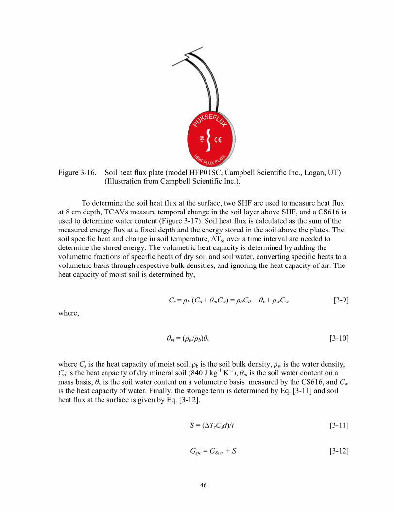
46

Figure 3-16. Soil heat flux plate (model HFP01SC, Campbell Scientific Inc., Logan, UT)

(Illustration from Campbell Scientific Inc.).

To determine the soil heat flux at the surface, two SHF are used to measure heat flux at 8 cm depth, TCAVs measure temporal change in the soil layer above SHF, and a CS616 is used to determine water content (Figure 3-17). Soil heat flux is calculated as the sum of the measured energy flux at a fixed depth and the energy stored in the soil above the plates. The soil specific heat and change in soil temperature, ∆Ts, over a time interval are needed to determine the stored energy. The volumetric heat capacity is determined by adding the volumetric fractions of specific heats of dry soil and soil water, converting specific heats to a volumetric basis through respective bulk densities, and ignoring the heat capacity of air. The heat capacity of moist soil is determined by,

Cs = ρb (Cd + θmCw) = ρbCd + θv + ρwCw [3-9]

where,

θm = (ρw/ρb)θv [3-10]

where Cs is the heat capacity of moist soil, ρb is the soil bulk density, ρw is the water density, Cd is the heat capacity of dry mineral soil (840 J kg-1 K-1), θm is the soil water content on a mass basis, θv is the soil water content on a volumetric basis measured by the CS616, and Cw is the heat capacity of water. Finally, the storage term is determined by Eq. [3-11] and soil heat flux at the surface is given by Eq. [3-12].

S = (∆TsCsd)/t [3-11]

Gsfc = G8cm + S [3-12]

47

Figure 3-17. Placement of heat flux plates (Illustration from Campbell Scientific Inc.).

3.4.4. DTS

Digital temperature sensing systems (DTS) were developed in the 1980s for fire monitoring, pipeline monitoring, and other industrial applications (Dakin et. al., 1985; Kurashima et al., 1990; Tyler et al., 2009). In 2006, Raman spectra DTS using fiber-optic cables became a promising and applied tool for hydrologic sciences to track thermal pulses, estimate fluid fluxes, trace surface water-ground water exchange, and estimate groundwater recharge, amongst other uses. DTS systems collects temperature of air, water, and solid media at much greater spatial and temporal resolutions than conventional instrumentation. DTS systems rely on Raman spectra scattering (Smith and Dent, 2006) and the known speed of light within an optical fiber to calculate the average temperature integrated over a specified length of fiber. DTS systems measure temperature in the fiber by pulsing a laser and timing the return signal, thus allowing multiple and frequent temperature measurements rather than a single measurement (Figure 3-18). Commercially available DTS systems can measure temperatures at spatial intervals as short as 1 m and as frequent as 10 s. For more detailed descriptions of the theory and operation of fiber optic DTS instruments, see publications by Selker et al. (2006) and Tyler et al. (2009).

Figure 3-18. Schematic of DTS system

Many configurations are available for fiber optics including different protective coverings, fillers, and number of fibers. However, two types of fiber optic cables were used in the lysimeters. The first (single fiber [1F], AFL) cable has 1 fiber surrounded by a polymer

48

buffer tube, an Aramid strength member, and an outer protective jacket. The AFL fiber optic (FO) cable is very thin, flexible, and fragile. Great care must be taken to not break the fiber. The second FO cable is a BRUGG FO (4F) cable which has 4 fibers covered with a gel-filled steel loose tube, reinforced with steel wires, and an outer protective jacket. The BRUGG cable is more durable than the AFL cable. The steel wires add memory to the BRUGG cable, requiring careful shaping to allow desired placement and orientation.

Figure 3-19. Cross section showing outer protective jackets and fibers of A) AFL Fiber

Optic (1F) cable; and B) BRUGG Fiber Optic (4F) cable.

3.5. Soil Physical Properties

Soil is the growth medium for living organisms and interacts with the atmosphere above and the strata below. Soil is the bio-physical-chemical reactor that breaks down waste products into nutrients for microorganisms and plants. Soil is defined as the weathered and fragmented outer layer of the earth and is formed through disintegration and decomposition of rocks by physical and chemical processes (Hillel, 1998). Natural soil is not homogeneous but is continually changing due to its dynamic interactions with the atmosphere and its role as a growth medium. As a result of these processes, soil will begin to develop, age, and form its own characteristics. There are many methods that can be applied to understand soil formation processes through physical, chemical, and biological processes.

3.5.1. MRT

Soil and root imagery is obtained using a root scanner (CI-600, CID Inc., Camas, WA), and a an acrylic mini-rhizotron tube (MRT) (6.35 cm OD, 3.1 mm wall thickness). Scanner size is 6.4 cm diameter x 34.3 cm length. The MRT is used to investigate soil particle movement and root growth. The system is a modified scanner, similar to those for flatbed scanners, that allows a head rotation of 345 º. An image is obtained when the scanner head is inserted into the MRT and the scanning program is started on the computer. The scan head will automatically rotate creating an image (21.58 cm (w) × 19.56 cm (l) size with maximum resolution of 1200 dpi or 188 million pixels) of the soil and roots in 5 to 15 s. However, initial scans revealed that the image quality did not improve significantly beyond 200 dpi. The scanner is moved progressively into the MRT to obtain images at different depths.

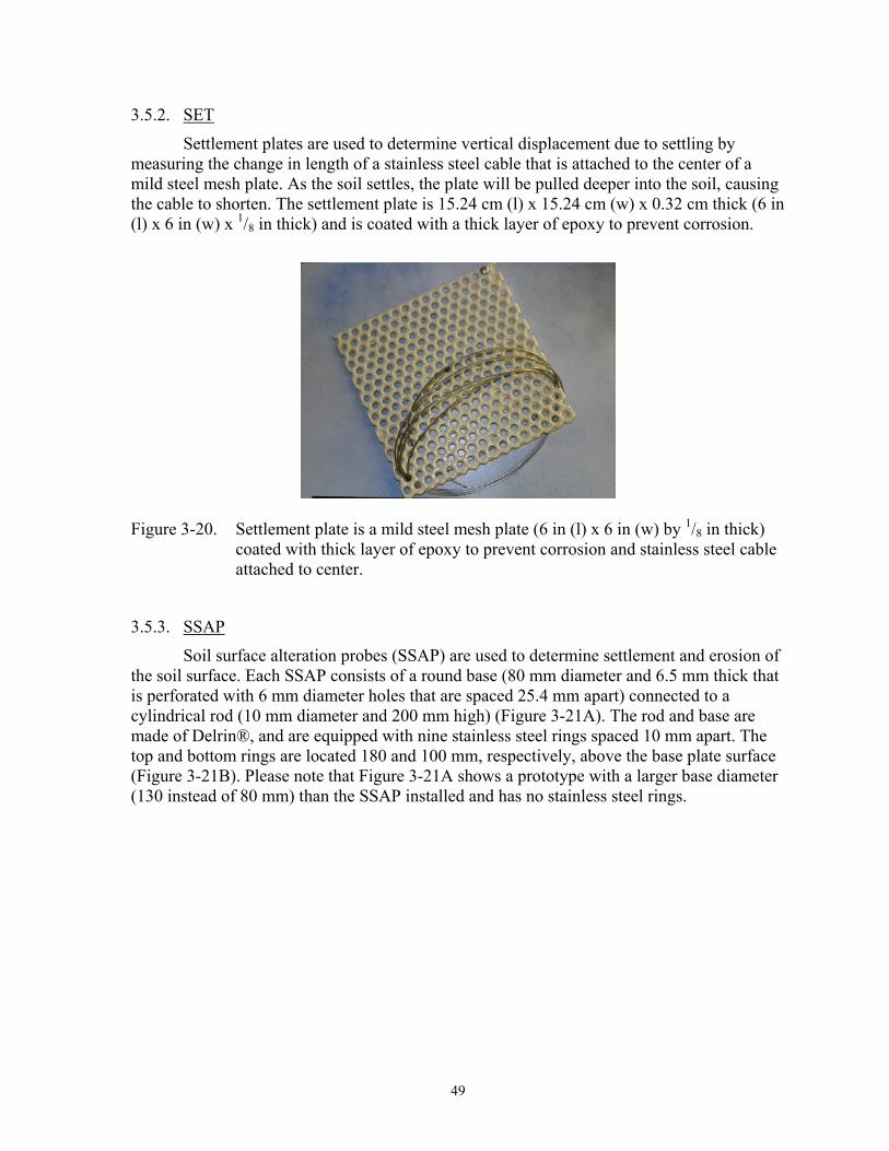
49

3.5.2. SET

Settlement plates are used to determine vertical displacement due to settling by measuring the change in length of a stainless steel cable that is attached to the center of a mild steel mesh plate. As the soil settles, the plate will be pulled deeper into the soil, causing the cable to shorten. The settlement plate is 15.24 cm (l) x 15.24 cm (w) x 0.32 cm thick (6 in (l) x 6 in (w) x 1/8 in thick) and is coated with a thick layer of epoxy to prevent corrosion.

Figure 3-20. Settlement plate is a mild steel mesh plate (6 in (l) x 6 in (w) by 1/8 in thick) coated with thick layer of epoxy to prevent corrosion and stainless steel cable attached to center.

3.5.3. SSAP

Soil surface alteration probes (SSAP) are used to determine settlement and erosion of the soil surface. Each SSAP consists of a round base (80 mm diameter and 6.5 mm thick that is perforated with 6 mm diameter holes that are spaced 25.4 mm apart) connected to a cylindrical rod (10 mm diameter and 200 mm high) (Figure 3-21A). The rod and base are made of Delrin®, and are equipped with nine stainless steel rings spaced 10 mm apart. The top and bottom rings are located 180 and 100 mm, respectively, above the base plate surface (Figure 3-21B). Please note that Figure 3-21A shows a prototype with a larger base diameter (130 instead of 80 mm) than the SSAP installed and has no stainless steel rings.

50

Figure 3-21. A) Top view of the SSAP prototype (larger base, rod without stainless steel

rings); and B) final SSAP design and installation sketch (SSAP designed by John Healey).

Surface settlement is determined by measuring the distance between the top ring on each SSAP and a fixed reference level (L-shaped aluminum bar). Two parameters for each measurement are obtained: 1) distance from the top ring of the probe to the reference level and 2) number of rings visible above the soil surface. For parameter 1, a metal ruler (Figure 3-22A) is used to measure the distance between the top ring of the probe and the surface of the horizontal leg of the L-shaped aluminum rod, representing the reference level. For parameter 2, the number of rings visible above the soil surface is counted (Figure 3-22B). First, a change in distance with time between a marker on the SSAP and the reference level indicates that the SSAP moved vertically up or down relative to the reference level, which indicates vertical movement of the lysimeter soil surface. Second, a change in the number of visible rings indicates soil deposition or erosion on the soil surface. An increase in the number of visible rings indicates erosion, and a decrease indicates deposition.

Figure 3-22. SSAP in the soil with nine stainless steel rings as markers and A) measuring

distance between top ring and reference level with the metal ruler resting on horizontal leg of the L-shaped aluminum rod and B) counting number of visible rings (taken on the lysimeter 1 on Sept. 16, 2008).

51

3.6. Gas and Water Sampling This section describes the instruments used to measure carbon dioxide in the soil pore

and how pore water will be sampled.

3.6.1. CO2

The CO2 sensors are designed to measure carbon dioxide in harsh and humid environments (CARBOCAP Carbon Dioxide Transmitter Series GMT220, Vaisala Instruments, Woburn, MA). The CO2 sensor is easy to install, has interchangeable probes for several measurement ranges, and is easy to maintain. The housing is dust- and waterproof to IP65 standards. The critical parts of the sensor are made of silicon and gives the sensor stability over time and temperature. Model type GMT222 CO2 sensor measures 0 to 3000 ppm CO2 and model type GMT221 measures 0 to 2% CO2 (0 to 20,000 ppm CO2). The output is in volts. A 10:1 voltage divider is used to reduce the output voltage of the transmitter to an acceptable range of the datalogger; and a multiplier is applied to determine the % CO2 [Eq. 3-13] and ppm CO2 [Eq. 3-14]. For more accurate CO2 values, CO2 measurements can be corrected for pressure and temperature.

CO2_pct = CO2_volt * 0.002 [3-13]

CO2_ppm = CO2_pct*1000000 [3-14]

Figure 3-23. Dimensions and components of CO2 sensors (CARBOCAP Carbon Dioxide

Transmitter Series GMT220, Vaisala Instruments, Woburn, MA) (Illustration from Vaisala Instruments).

52

3.6.2. SSSS

Stainless steel solution samplers (SSSS) are used to extract pore water from unsaturated soil for water quality analyses. The single-chamber solution sampler (model SW-074, Soil Measurement Systems, Tucson, AZ) is made of stainless steel porous tube (2.22 cm OD) with two stainless steel tubes (3 mm OD) inserted into the body of the sampler. There are two lengths of SSSS where the short (top SSSS in Figure 3-24) and long (bottom SSSS in Figure 3-24) samplers have porous cylinders that are 20 and 50 cm in length, respectively. There are are also two lengths of stainless steel tubing that extrude 10.2 and 17.7cm from the porous sampler. The stainless steel tubes are connected to flexible Teflon tubing (0.125 OD and 0.030 ID, model PFA-T2-030-100, Swagelok, Tempe, AZ) using stainless steel connectors (model SS-200-6, Swagelok, Tempe, AZ). The short stainless steel tube is a tube that is used for maintaining vacuum in the sampler and conveying pore water into the porous tube. The long stainless steel tube is a vacuum release tube that is used to release vacuum levels (Figure 3-24). Solutions samplers are placed in the soil at a 10º to the horizontal, with the long tubing at the top, placing the solution withdrawal tubing to be located at the base of the sampler (Figure 4-13B). This orientation facilitates water collection at the closed end of the sampler. Bubbling pressure is approximately 600 cm H2O. The Teflon tubing runs through the portholes and is sealed with compression fittings (model RSP-200-W and RSB-200, Remke, Wheeling, IL).

Figure 3-24. Short and long stainless steel solution samplers (SSSS) with 20 and 50 cm

porous cylinders shown on top and bottom. Each SSSS has two stainless steel tubing that extrude 10.2 and 17.7 cm from the porous sampler.

3.6.3. Tracers

Tracers play an important role in understanding flow and transport processes in the subsurface. Particularly, tracers are used to measured flow velocity and travel time, flow direction, and hydrodynamic dispersion. Several tracers such as isotopes, anions, fluorobenzoates, polyaromatic sulfonates, and dyes have been recommended and used for hydrological investigations. However, some tracers sorb to sediments and may degrade during the investigation period. An ideal water tracer moves in a manner similar to water (i.e., conservative in behavior), has low background concentration, and is not sensitive to changes in solution chemistry.

53

Isotopic tracers are used by substituting one or more atoms of the molecule of interest with the same chemical element but with a different isotope. It will contain the same number of protons, thus not changing its chemical reaction with other compounds, but the difference in neutrons will allow it to be detected separately from the other atoms of the same element using neutron magnetic resonance spectroscopy (NMR). Once the system is ‘labeled’ with an isotope, tracking its passage through a system is possible. A specific isotopic tracer is nitrogen-15 which is a stable, non-radioactive isotope of nitrogen and is regularly used in agricultural research for plant nutrition and soil fertility. Nitrogen and nitrogen isotopic compositions in soil and water is controlled by biologically-mediated reactions (e.g., assimilation, nitrification and denitrification). Nitrification produces nitrate (NO3

-) through the oxidation of ammonium (NH4

+) under aerobic conditions. Besides N2 (g), nitrate is the most stable form of nitrogen and is present in most groundwater. Denitrification occurs under anaerobic conditions by bacteria and plant assimilation. Analysis of N-15 with O-18 provides information about nitrates in water and soils.

Nitrification: NH4

+ + 2O2 = NO3- + 2H+ + H2O [3-15]

Denitrification:

NO3- + 5/4CH2O = 1/2N2 +5/4HCO3

- +1/4H+ +1/2H2O [3-16]

Studies have reported that bromide, pentafluorobenzoic acid (C6F5CO2H or PFBA), and 2,6-difluorobenzoic acid (F2C6H3CO2H2 or 2,6-DFBA) move at a similar rate as water in most soil conditions (Bowman, 1984; Bowman and Gibbens, 1992; Jaynes, 1994). Contrarily, most dye tracers sorb to soils to some extent. The sorption of these tracers (bromide, PFBA, 2,6-DFBA) in Arizo has not been tested. However, many investigators have reported that bromide, PFBA, and 2,6-DFBA showed no sorption under most soil conditions and thus are suitable for tracing water movement in soils (Bowman, 1984; Bowman and Gibbens, 1992; Mayes et al., 2003).

Despite non-conservative behavior, dyes are often used as water tracers because of their unique properties—visibility, ease of detection, low background concentration, and simple technology. Among dye tracers tested in sandy soils, Food, Drug, and Cosmetics (FDC) Green No. 3 demonstrated relatively low sorption levels (Mon et al., 2006). For the Arizo soils used in the lysimeters, analyses of sorption isotherms for FDC Green No. 3 shows a maximum sorption capacity of 0.338 mmol kg-1 and a Langmuir coefficient of 10.707 kg-1 (Figure 3-25A). A column experiment, conducted under water-saturated conditions to determine the retardation factor for the dye compared to that of NO3

-, showed that the retardation factor for the dye was 1.89, where the retardation factor for NO3

- was 0.99 (Figure 3-25B).

54

0

0.1

0.2

0.3

0.4

0.5

0 0.5 1 1.5 2 2.5mmol L-1

mm

ol k

g-1

FDC Green No. 3

A)

0.0

0.2

0.4

0.6

0.8

1.0

1.2

0 2 4 6 8 10 12 14 16Pore Volume

C C

0-1

FDC Green No.3

NO3B)

Figure 3-25. A) FDC Green No. 3 sorption curve for 25-80 cm soil. B) FDC Green No. 3

and NO3- breakthrough curves for 25-80 cm soil.

3.7. Meteorological Variables The extended open path eddy covariance (OPEC) system and directional anemometer

and micro-insrument tower (DAMIT) are used to measure micrometeorological components needed to measure actual evapotranspiration and to close the energy balance.

3.7.1. OPEC

The eddy covariance system consists of a datalogger, a three-dimensional anemometer (model CSAT3, Campbell Scientific, Inc.), a open path infrared gas analyzer (IRGA; model LI-7500, Licor, Inc.), a temperature and humidity probe (model HMP45C, Cambell Scientific, Inc.), net radiometer (model NR-LITE, Kipp and Zonen), tipping bucket rain gage, soil heat flux plates (model HFP01SC, Campbell Scientific, Inc.), soil temperature probes (model TCAV, Campbell Scientific, Inc.), and soil water content sensors (model CS616, Campbell Scientific, Inc.). This system allows measurements of carbon dioxide flux, latent heat flux, sonic and computed sensible heat flux, momentum flux, temperature, humidity, wind vectors (speed and direction), net radiation, soil heat flux, soil temperature, and soil water content.

3.7.1.1. CSAT3

The CSAT3 is a three dimensional ultrasonic anemometer that measures wind speed in three dimensions using three pairs of non-orthogonally oriented transducers to sense the horizontal wind by transmitting and receiving ultrasonic signals (Figure 3-26). The wind speeds are transformed to orthogonal wind components, ux, uy, and uz and are referenced to the anemometer head. The speed of sound (c) or the sonic virtual temperature (Ts) is directly related to the air density, using temperature and humidity, and is determined by combining the out and back time-of-flight measurements. The speed of sound is measured on all three axes and then averaged to find a single value. It is also corrected for crosswinds or wind blowing normal to the sonic measurement path. By measuring the average wind speed and direction, the turbulent fluctuations of horizontal and vertical wind speeds and momentum flux can be determined. The sensible, latent heat, and carbon dioxide flux can also be determined using the covariance between the humidity and wind speed. The anemometer head is 47.3 cm (l) x 42.4 cm (h) and weighs 1.7 kg (3.7 lb). The transducers are 0.64 cm

55

(0.25 in) diameter and 60° from the horizontal. The right-handed orthogonal coordinate system is oriented with the CSAT3 pointing into the negative x direction, so that if the anemometer is pointing into the wind, it will report a positive ux wind. Measurement resolution for ux, uy, uz, and c are 1, 1, 0.5, and 15 mm s-1 and the reporting ranges are 32.8, 65.5, 8.2, and 300 mm s-1, respectively.

Figure 3-26. CSAT3 three dimensional sonic anemometer (Campbell Scientific Inc.,

Logan, UT) (Illustration from Campbell Scientific Inc.). 3.7.1.2. LI-7500

The LI-7500 (model LI-7500, LI-COR Biosciences, Lincoln, NE) is a high speed precision, non-dispersive infrared gas analyzer that measures the concentration of carbon dioxide and water vapor. It is used with a sonic anemometer to determine CO2 and H2O fluxes. The flux, Fc of a gas c, is given by Fc = w’pc’ where c’ is the density fluctuations of the gas (mmoles m-3) and w’ is the vertical wind velocity fluctuations (m s-1). The precision is 0.16 ppm CO2 and 0.0067 ppt H2O.

Figure 3-27. Components of the LI-7500 (model LI-7500, LI-COR Biosciences, Lincoln,

NE) (Illustration from LI-COR Biosciences).

56

3.7.1.3 HMP45C

The HMP45C (model HMP45C, Campbell Scientific, Inc., Logan, UT) is a temperature and relative humidity probe that measures the air temperature and relative humidity using a Platinum Resistance Temperature detector (PRT) and a Vaisala HUMICAP® 180 capacitive relative humidity sensor (Figure 3-28). It is 25.4 cm (10 in) long with a 2.5 cm (1 in) body diameter, operates from -40° to 60°C and has a relative humidity accuracy of +2-3%. Measurements can be used to determine air and vapor density.

Figure 3-28. HMP45C temperature and relative humidity probe (model HMP45C,

Campbell Scientific, Inc., Logan, UT) (Illustration from Campbell Scientific Inc.).

3.7.1.4 Net Radiometer

The net radiometer is a high-output thermopile sensor which measures incoming and outgoing long- and short-wave radiation (model NR-LITE Net Radiometer, Campbell Scientific Inc., Logan, UT). Incoming radiation includes direct (beam) and diffuse solar radiation and long-wave irradiance from the sky. Outgoing radiation includes reflected solar radiation and terrestrial long-wave radiation. The result is a measure of the total net radiation (W m-2) using the difference between incoming radiation measured by the upward facing sensor and the outgoing radiation measured by the downward facing sensor. The sensor is 8.0 cm (3.1 in) in diameter and weighs 635 g (23 oz) with a spectral range of 0.2 to 100 μm and a directional error less than 30 W m-2.

Figure 3-29. NR-LITE net radiometer (model NR-LITE, Campbell Scientific Inc., Logan,

UT) (Illustration from Campbell Scientific Inc.).

57

3.7.1.5 Rain Gage

The tipping bucket rain gage (model TE525WS-L, Campbell Scientific, Inc., Logan, UT) measures in 0.254 mm (0.01 in) increments with an accuracy of +1% at rates up to 2.54 cm hr-1. Precipitation funnels into a bucket that tips over when filled and a magnetic switch is activated to count the number of tips using a datalogger to determine the volume. The rain gage has an orifice diameter of 20.3 cm (8 in), a height of 26.7 cm (10.5 in), and is made of anodized aluminum.

Figure 3-30. TE525WS-L Texas Electronics 8in rain gage (Illustration from Campbell

Scientific Inc.). 3.7.1.6 CS616

Please see section 3.2.3.

3.7.1.7 TCAV


3.7.1.8 SHF


3.7.2. DAMIT

The directional anemometer and micro-instrument tower (DAMIT) is a near-ground surface monitoring system that consists of 1) wind sentry set that measures wind speed and direction 10 cm above ground surface; and 2) a temperature and relative humidity micro-instrument tower made from several stacked relative humidity and temperature sensors (model SHT-75, Sensirion, Westlake Village, CA) located at 5, 10, 25, and 50 cm above the ground surface (igure 4-19). The system is installed outside of lysimeter 3.

The wind sentry set has a 3-cup anemometer and wind vane that is mounted on a crossarm (model 03002 wind sentry set, Campbell Scientific, Inc., Logan, UT). The rotation of the anemometer cups produces an AC sine wave that is proportional to wind speed. The frequency of the AC signal is a pulse counted converted to wind speed using a datalogger. The range of wind speed measured by the anemometer is 0 to 50 m s-1 (0 to 112 mph) with an

58

accuracy of +0.5 m s-1 (+1.1 mph). The wind direction is determined by the potentiometer that is connected to the 360° rotating wind vane. The output signal is an analog voltage that is directly proportional to the azimuth of the wind direction. The wind direction accuracy is +8°.

Figure 3-31. A 3-cup anemometer and a wind van mounted on a cross arm (model 03002

wind sentry set, Campbell Scientific Inc., Logan, UT) (Illustration from Campbell Scientific Inc.).

The micro-instrument tower has four relative humidity and temperature sensors. The sensors integrate elements with signal processing in a very compact form, while providing a fully calibrated digital output. Relative humidity is measured with a unique capacitive sensor element and has an accuracy of +3.0% with a typical resolution of 0.05%. Temperature is measured with a band-gap sensor and has an accuracy of +0.4°C, a range from -40 to 123.8°C, and has a resolution of 0.01°C.

59

Figure 3-32. Dimensions of relative humidity and temperature sensor SHT75 (Illustration

from Sensirion).

60


61

4. INSTRUMENT LAYOUT AND INSTALLATION

Approximately 152 sensors and instruments were installed in each lysimeter. Table 4-1 lists the number of each sensors in each lysimeter. In addition to the sensors installed in the lysimeter, immediately east of the main room for lysimeter 3, six TDR probes were installed in the adjacent natural soil at 50 cm depth intervals from ground surface, and nine thermocouples were installed at depths of 5, 10, 25, 75, 100, 150, 200, 250, and 300 cm (Table 4-2 and Table 4-3). These sensors were installed so that conditions inside the lysimeter tank could be directly compared to conditions in undisturbed soil. The DAMIT system is installed immediately above lysimeter 3, on the north side, and an OPEC system is installed 112 m W of lysimeter 1.

Figure 4-1. Aerial photograph of the lysimeter facility in Boulder City, NV, showing

location of instruments installed in adjacent natural soil (yellow star), OPEC (blue triangle) and DAMIT (light blue box).

Table 4-1. Catalogue and number of instruments at each depth for each lysimeter. Depth [cm] CO2 CS616† DPHP DTS

Loops DTS Pole‡ ECH2O HDU MRTh MRTv‡ NAT‡ SET SHF SSAP SSSS STherm TCAV TDR TPHP Sub-

total

0 1 1 1 1 3 4& 11 5 1 2 4 1 1 9

10 1 4 2 4 4 15 25 2 4 1 4 4 15 50 1 4 4 1 4 4 18 60 1 1 2 75 2 1 4 4 1 4 2 18 90 1 2 3

100 4 2** 4 1 4 2 17 140 2 2 150 4 4 1 4 4 17 190 2 2 200 2 1 2 2 2 9 250 2 2 2 2 8 290 6 6

Sub-total 3 1 14 8 1 2 32 3 1 1 6 2 3 26 4 1 26 18 152

† - CS616 was installed only in lysimeter 1.

‡ - One vertical tube extends through entire depth of lysimeter.

& - This is a TPHP Cluster between 0-5 cm at approximately 1 cm interval.

* - In Lysimeter 1, there is a total of 8 TPHPs instead of 18 and 24 DPHPs instead of 14. This results in 2, 2, 4, and 4 DPHPs at 10, 25, 50, and 75 cm.

** - DTS loop is at 95 cm.

62

63

Table 4-2. Comparison of temperature measured in lysimeter and adjacent natural soil east of lysimeter 3 (data stored as BC_Lys3_TC.dat). Gray cells indicate temperature measured at same depth.

Lysimeter Soil

Adjacent Natural Soil

Depth [cm] DPHP DTS

Loops DTS Pole‡ ECHO HDU STherm TCAV TPHP TC

0 1 4& 5 1 2 4 1 1

10 1 4 4 1 25 2 4 1 4 1 50 1 4 1 4 1 60 75 2 1 4 1 2 1 90

100 4 2 4 1 140 150 4 1 4 1 190 200 2 2 1 250 2 2 1 290 1**

Sub-total 14 9 1 2 32 4 1 18 9

† - CS616 was installed only in lysimeter 1. ‡ - One vertical tube extends through entire depth of lysimeter. & - This is a TPHP Cluster between 0-5 cm at approximately 1 cm interval. * - In Lysimeter 1, there is a total of 8 TPHPs instead of 14 and 24 DPHPs instead of 14. This results in 4, 4, 2, and 2 DPHPs at 75, 50, 25, and 10 cm. ** - This thermocouple is actually at 300 cm depth. Note: This data is collected in BC_Lys3_TC.dat.

64

Table 4-3. Comparison of temperature measured in lysimeter and adjacent natural soil east of lysimeter 3. Gray cells indicate water content measured at same depth.

Lysimeter Soil Adjacent Natural Soil Depth [cm]

CS616† TDR TDR

0 5

10 1 4 25 4 50 4 1 60 75 4 90

100 2 1 140 150 4 1 190 200 2 250 2 290

Sub-total 1 26 3 † - CS616 was installed only in lysimeter 1. ‡ - One vertical tube extends through entire depth of lysimeter. & - This is a TPHP Cluster between 0-5 cm at approximately 1 cm interval. * - In Lysimeter 1, there is a total of 8 TPHPs instead of 14 and 24 DPHPs instead of 14. This results in 4, 4, 2, and 2 DPHPs at 75, 50, 25, and 10 cm.

4.1. Instrument Nomenclature

An identification system was developed for instrument placement and portholes through which instruments are wired. It was necessary to classify portholes so that wiring of instrument cables could be identified, especially given that no portholes are shallower than 60 cm; thus, instruments were not necessarily strung through a porthole adjacent to the instrument. The location of the sensors is identified by lysimeter room#_depth_quadrant. For example, an instrument placed at 50 cm depth in the NW quadrant of lysimeter 1 (or room 1) is identified as being located at R1_50_NW. Portholes are identified by lysimeter#_quadrant/port#_depth. Portholes are numbered one to six in a clockwise direction for each of four clusters for each depth. For instance, a port numbered R1_NW1_D295 identifies a porthole located in lysimeter 1 in the NW quadrant and is the first porthole in the quadrant at a depth of 295 cm (Appendix C). Placement of instruments was accomplished using plan view maps showing instrument type and serial number for each depth (Appendix C, Figure C-1). A table is attached to each map designating the port through which the instrument cable is wired (Appendix C, Table C-1 to

65

Table C-17).

4.2. TDR, FDR, ECH2O, DPHP, TPHP, HDU, Stherm, TCAV, SHF, and SSSS Above 25 cm, instrument were placed at 0, 5, and 10 cm depths. The vertical spacing

between instrumented layers from 25 to 100 cm depth is 25 cm and between 100 cm and 300 cm depths, the vertical spacing is approximately 50 cm. The typical suite in an instrumented layer includes 16 sensors placed in the horizontal plane with four sensors in each of four quadrants: an HDU, a TDR, either a DPHP or a TPHP, and an SSSS (Figure 4-2; Figure C-1M). Instruments were positioned radially toward the center of the lysimeter with the center of the instrument at 56.5 cm (half the lysimeter radius) from the wall of the lysimeter. Full instrument suites exist at four depths between 50 and 150 cm (Figure C-1F, H, K, and M). At depths of 200 and 250 cm, instruments were installed using only two quadrants at each depth. At 200 cm, sensors were placed in quadrants II and IV (SE and NW respectively) (Figure C-1O) and at 250 cm, sensors were placed in quadrants I and III (NE and SW, respectively) (Figure C-1P).

Near the ground surface, instrument density was higher because a greater spatial and temporal variability of heat and moisture occur in shallower soil zones. The shallowest instruments were placed at approximately 5 cm depth (Figure 4-3). This instrument suite has one HDU in each quadrant; an ECH2O, SHF and corresponding TCAV in quadrants I and III; a soil thermistor (STherm or model 108L) positioned between quadrants I and II on the east-west centerline; and a TPHP cluster or “Titanic” in quadrant II (Figure 4-3; Figure C-1C). The Titanic is oriented vertically instead of in the plane and has four TPHPs aligned in a downward trend.

Certain instruments, such as the soil heat flux plates (SHF) and averaging thermocouples (TCAV) were only placed near the surface (i.e., upper 10 cm of soil) (Figure 4-4). Lysimeter 1 included a CS616 which was not installed in lysimeters 2 and 3. The FDR was placed in SW quadrant (quadrant III) at the same depth as the SHF to measure moisture content (Figure 4-4). Also, at depths of 10 and 25 cm, solution samplers were not used so the instrument suite consisted of an HDU, a TDR, and either a DPHP or a TPHP in each quadrant (Figure C-1D and E). TPHP sensors allow for the measurement of water content and thermal properties at 6 mm intervals, and therefore, were installed at shallower depths where possible. In addition, the TPHP sensors became available during soil installation phase, and thus the decision was made to augment the DPHP instruments with TPHP sensors in the top 75 cm.

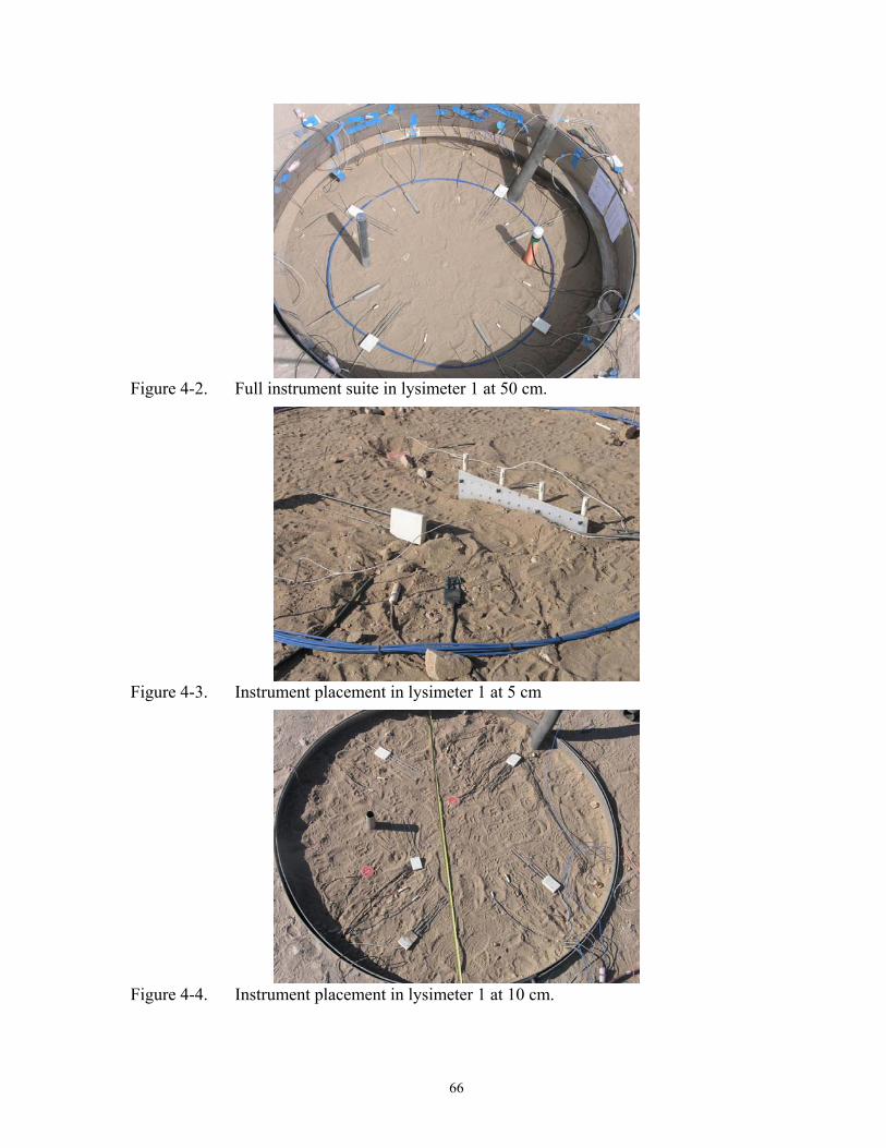
66

Figure 4-2. Full instrument suite in lysimeter 1 at 50 cm.

Figure 4-3. Instrument placement in lysimeter 1 at 5 cm

Figure 4-4. Instrument placement in lysimeter 1 at 10 cm.

67

4.3. DTS, NAT, and vertical MRT

Three types of instruments were installed through the entire depth of the lysimeters: neutron probe tube, DTS pole, and the vertical MRT (Figure 4-5). The neutron access probe was installed vertically (with 6.35 cm of NAT protruding from the filled lysimeter surface) and the vertical MRT was installed at a 31º angle to the vertical. This offset from vertical was made to improve viewing of roots as they grow through the soil.

Figure 4-5. DTS Pole, Vertical Mini-Rhizotron Tube (MRT), and Neutron Access Tube

(NAT) extend through the entire vertical depth of each lysimeter. DTS pole, vertical MRT, and NAT installed in empty lysimeter 2.

4.4. DTS The AFL FO (1F) and BRUGG FO (4F) cables were installed in the each lysimeter.

The AFL FO cable was wrapped around a vertical pole to measure high-resolution vertical temperature gradients, and the BRUGG FO cable was placed in loops at 6 depths to measure temperatures on a horizontal plane at regular depths. The DTS pole is a threaded 5.08 cm (2 in, nominal) schedule 40 PVC pipe wrapped with a 900 micron cable containing a simplex tight-buffered 50/125 multi-mode fiber (AFL Telecommunications, Duncan, SC). The pipe, 6.03 cm (2.375 in) OD, has standard threads with a thread pitch of 4.5 threads per cm (11.5 threads per in). The inside of the pipe is filled with insulating foam to prevent internal heat convection from interfering with temperature measurements (Figure 4-6A). The fiber is seated in the threads, with a diameter of rotation similar to the outside diameter of the pipe. This configuration, shown in Figure 4-6B, provides a vertical resolution of 1.17 vertical centimeters per meter of optical fiber.

68

Figure 4-6. DTS pole showing A) insulation foam; and B) threat pitch of 4.5 threads per

cm glued onto schedule 40 PVC pipe.

DTS loops were installed to study the wall effects on the thermal regime of the lysimeters. DTS loops are concentric loops at different depths of BRUSteel (BRUGG) Flexible Mini Fiber Optic Cable 4F (an armored cable with duplexed loose-tube 50/125 multi-mode fibers, Brugg Kabel, Brugg, Switzerland). The diameter of the inner loop is 1 m and outer loop is 1.5 m. The depths of installation of the inner loops in the lysimeter are 5, 25, 50, 75, 95, and 200 cm. Outer loops are present at 25 and 95 cm depths. The different diameter loops were used to estimate the potential for lateral heat movement between the soil and the lysimeter wall. Each loop was centered as closely as possible in the lysimeter, with the larger loop placed 13 cm from the lysimeter wall, and the smaller loop placed 38 cm from the wall (Figure C-1J). Each fiber optic DTS deployment includes a free length of cable (approximately 30–50 m) on either end of the measurement area (at the bottom 150 cm porthole and at the top 60 cm porthole). This length of cable is required to calibrate the installation prior to making any measurements. A schematic diagram of the DTS loops are shown in (Figure 4-7) and a photo of the DTS loops during installation is shown in Figure 4-8.

5 cm

25 cm

50 cm

75 cm

95 cm

200 cm

Outer loop (d=2 m)

Inner loop (d=1.5 m)

Cable end 1

Cable end 2 Figure 4-7. Installation design for optical fiber loops.

69

Figure 4-8. DTS loops being installed at 95 cm in a lysimeter 2.

4.5. MRT Three horizontal (MRTh) and one vertical (MRTv) were installed in each lysimeter.

Lysimeter ports were modified to accommodate the larger diameter clear acrylic pipe through the lysimeter. The MRTh were installed at depths of 60, 100, and 150 cm, oriented NW to SE through porthole 3. The MRTv was placed at a 31° angle from SW porthole 4. While soil was being installed, the extruding portion of the MRTv was protected with rubber tubing to prevent accidental scratching. However, the MRTv in lysimeter 1 broke at 50 cm depth and was repaired with a clear outside sleeve (ca. 6.35 cm ID x 50 cm long). After installation, the complete length of inside each MRT was cleaned with a terry cloth and mild soap to remove excess soil and the ends were covered with a plastic cap to prevent dust from entering the tube. MRTh were cut such that 10 cm length was extruding from the lysimeter wall. The MRTv was cut approximately 10 cm above ground and then covered with a painted-white PVC tubing to protect the MRT from the sun and other disturbances.

70

Figure 4-9. Repaired vertical MRT with sleeve at 50 cm depth in lysimeter 1 and broken

MRT that was removed and replaced with repaired MRT.

4.6. SET Two settlement plates each were placed at depths of 90, 140, and 190 cm in quadrants

1 and 3, 2 and 4, and 1 and 3, respectively, and their cables were fed through portholes at 60, 100 and 150 cm, respectively (Figure 4-10). The distances of the SET from the inner wall of the lysimeters were 22.5, 30, and 30 cm, respectively, meaning that the angles of the cables were 36.9º in each case. The cable was placed inside a rigid outer tubing or “cable housing” so that the cable could move freely while being held in place with the compression fitting in the porthole. Approximately 100 mm of cable protrudes perpendicular out of the lysimeter and is periodically measured using a digital caliper. The digital caliper is placed parallel to the cable, so that the caliper’s inner diameter measurement stops are against the inside portion of the cable housing and cable tip (Figure 4-11). Light tension is placed on the caliper adjustment wheel to make sure the cable is straight. (Note: The cable at 60 cm depth is not perpendicular because the frame structure of the lysimeter room obstructs it and because measurements are made at an angle, it is more prone to error.)

71

Figure 4-10. Two settlement plates in the SE and NW quadrants at 190 cm depth in

lysimeter 2.

Figure 4-11. Photo of caliper instrument to measure settlement plates.

72

Table 4-4. Initial caliper measurements of settlement plates taken on June 12, 2008.

Lysimeter 1 Lysimeter 2 Lysimeter 3 Settlement Plate -------------------[mm] -------------------

NE_60 cm 105.22 102.40 102.48 SW_60 cm 101.97 100.47 101.60 NW_100 cm 102.48 102.68 100.71 SE_100 cm 104.43 101.47 102.93 NE_150 cm 102.10 103.57 103.86 SW_150 cm 101.75 100.43 101.70

4.7. SSAP

All nine SSAPs were installed on Jul. 18, 2008 with the upper surface of the base plate installed 100 mm beneath the soil surface. The L-shaped aluminum bar used as fixed reference level was attached to the ring flashing of the lysimeter when measurements were taken (Figure 3-22A; Figure 4-12). Table 4-5 provides the values of the initial measurement.

Figure 4-12. Arrangement of SSAP 7, 8 and 9 in lysimeter 3 with aluminum rod across the

lysimeter surface as reference base (on Sept. 16, 2008).

73

Table 4-5. Initial measurements of SSAPs from Jul. 18, 2008.

4.8. SSSS Four 20 cm length stainless steel solution samplers (SSSS) were installed at 50, 75,

100 and 150 cm and two 20 cm long SSSS were installed at 200 and 250 cm depth. Six SSSS of 60 cm length were installed at 290 cm depth. The sole purpose of the shorter SSSS is to extract pore water while the long SSSS near the lysimeter bottoms are primarily intended to create a specified constant matric potential using an applied vacuum in dry soils (Figure 4-13A and Figure C-1). The samplers were oriented with the closed end towards the center of the lysimeter and the open end (of stainless steel tubes) towards the sample porthole. Flexible 1/8” Teflon tubing is attached to the short and long stainless steel tubings with one pair wired through an adjacent porthole. The mid-points of SSSS were placed 57.5 cm from the lysimeter wall (50% of the radius) (Figure 4-13B).

The solution-vacuum manifold consists of a panel of 40 mL glass vials for pore water collection and one schedule 80 ½-in PVC pipe connected to a vacuum pump to establish a vacuum (Figure 4-14). The vacuum manifold was constructed so that solution samplers could be placed under vacuum individually, thereby allowing targeted pore water sampling by depth or quadrant. Each lysimeter has two solution-vacuum manifolds that are attached to the lysimeter at 180º from each other. Each PVC pipe was drilled and tapped to ¼-in National Pipe Thread (NPT) to accommodate ¼-in vacuum valve (model HVN2-N2U, PISCO, Bensenville, IL). Each manifold is connected to a central GAST vacuum pump thereby, placing both manifolds under identical vacuum levels. Compression fittings were secured on to the vacuum control valves situated along the length of the PVC pipe at the same depths as the portholes (i.e. one for each solution sampler).

Lysimeter SSAP # Distance [mm] # Rings

1 55 8

2 57 9

1

3 58 9

4 55 8

5 55 8

2

6 58 8

7 40 9

8 48 8

3

9 48 8

74

Figure 4-13. A) 50 cm long stainless steel solution samplers are installed at 295 cm depth

in lysimeter to create a vacuum; and B) using a wooden block to place stainless steel solution samplers at a 10° angle.

Figure 4-14. Stainless steel solution sampler manifold attached to one side of the lysimeter.

There are two SSSS manifolds per lysimeter.

From the SSSS, the vacuum/extraction line is routed through a two-hole rubber stopper to a glass vial mounted along-side a vacuum manifold (Figure 4-15). The vacuum release tube is connected to flexible Teflon tubing and sealed off with a pinch valve. A short length of Teflon tubing is routed through the other hole in the rubber stopper and is terminated into a compression fitting.

75

The two lines from the solution samplers are routed as follows:

• The short steel tube or the “extraction tube,” is connected to tubing (flagged red) and is routed to the vial;

• A Teflon tube connects the vial to the vacuum manifold; and

• The long steel tube or the “vacuum release tube” is connected to Teflon tubing (flagged white) and sealed with a pinch valve.

Figure 4-15. Routing of SSSS to solution manifold.

At the time of this writing, no pore water was available for sampling. However, the plan to operate the system is known, with operations to differ depending on purpose. The bottommost samplers are used to control unsaturated conditions. Thus, the vacuum level will be set at the approximate soil water potential as measured in the soil, in this case at 250 cm depth where the deepest HDUs are located (Table 4-1). In this way, the soil water potential would be approximately equal toward the base of the lysimeter, thus creating unit gradient conditions in the soil. Samplers installed at shallower depths, to be used specifically for sampling and analyzing soil pore water, will be placed at a vacuum level that facilitates a hydraulic gradient toward the sampler, such that water will collect in the porous tubing.

4.9. Tracers Tracers will be used to determine the hydrodynamics of the lysimeter soil and to track

the upward and downward movement and the mixing behavior of water in soil profiles. Five different tracers are applied on the lysimeter at 6 different depths including N-15 at 10 ppm at 5 cm in lysimeter 1 when the experiment starts; 2,6 DFBA and PFBA at 15 and 30 cm in all lysimeters; Br at 40 cm in all lysimeters; FDC Green No. 3 at 55 cm in all lysimeters; and N-15 at 210.5 ppm in lysimeter 2. Table 4-6 lists each tracer, depth of application, chemical form, amount of water used for solution, and target concentration. The amount of mass

76

needed for each tracer is determined using a volumetric water content of 0.20 cm3 cm-3 and an assumed minimum detectable tracer concentration. The tracer is dissolved in deionized water. A wire mesh with 178 squares is placed in the lysimeter over the soil and the solution volume is divided equally among all squares using precision pipettes (Eppendorf pipette, Eppendorf North America, Hauppauge, NY). See Appendix D for specific calculations.

Figure 4-16. Tracer application in lysimeter 1 of A) FDC Green No. 3 at 55 cm; and B)

PFBA at 30 cm. Table 4-6. Depth and mass of tracers applied in lysimeters 1, 2, and 3.

Lysimeter Depth Tracer Mass Chemical Form Water Target Conc.

[cm] [g] [mL] 1 1† 5 N-15 0.7 KNO3 1000 10 ppm N-15

2 1,2, and 3 15 2,6-DFBA 2.4 2,6-DFBA 1000 1 mg L-1 2,6 DFBA

3 1,2, and 3 30 PFBA 2.4 PFBA 1000 1 mg L-1 PFBA

1 15.01 Br 1000 5 mg L-1 Br 4

2 and 3 40 Br‡

12.01 Br 1000 5 mg L-1 Br

5 1,2, and 3 55 FDC Green No. 3 (dye) 12.01 FDC Green No.

3 (dye) 1050 5 mg L-1 Br

5 dry CaNO3 0 6 2 150-200 N-15

49.2 N-15 (KNO3) 890 210.5 ppm N-15

† Applied only lysimeter 1 when experiment begins. ‡ Calculated 80% of Br- in KBr-

To study the interaction between vegetation and the nitrogen reservoir in deserts of the southwestern U.S. (Walvoord et al., 2003), a 50 cm layer of N (200 mg kg-1 N) was created in lysimeter 2 using a total mass of 5.0 kg CaNO3 and 49.2 g N-15 (KNO3). The

77

compounds were divided into 5 equal portions. After each 10 cm thick layer of soil, CaNO3 prills (3 mm diameter) were broadcast on the surface. The dissolved N-15 was injected on the surface, dried, and mixed gently using a garden claw. The procedure was repeated five times to make a 50 cm thick layer of spiked N. Zones of application are given in Figure 4-17. In lysimeter 1, 0.3 g (1% of the total N in the soil) of N-15 as KNO3 will be applied at the soil surface when the experiment begins. This facilitates the study of the fate of N-15 in desert soils under natural conditions.

Figure 4-17. Schematic of N-15 application in lysimeters.

4.10. OPEC The OPEC is located 28.5 m (93.33 ft) directly west of the southern midpoint of

lysimeter 1. The rain gage and radiometer is located 3.2 m (10 ft) south and 3.2 m (10 ft) east of the eddy covariance tower.

Figure 4-18. Different instruments and components of the open path eddy covariance

(OPEC) system.

Lysimeter 1

150 cm

50 cm of N-15

100 cm

15 cm of N-15

285 cm

Lysimeter 2

78

4.11. DAMIT

DAMIT was installed in fall 2008 with the micro-instrument tower directly above north side of lysimeter 3 (Figure 4-19). The directional anemometer is located 2.7 m (8.9 ft) north of the micro-instrument tower (Figure 4-20). These sensors provide a better measure of the environmental conditions that are affecting the lysimeters.

Figure 4-19. Directional Anemometer and Micro-Instrument Tower (DAMIT).

Figure 4-20. Location of OPEC (blue triangle) and DAMIT (light blue rectangle) at the

SEPHAS lysimeter facility.

79

5. INSTRUMENT CALIBRATION

5.1. Weighing Lysimeter

Load cells were calibrated individually in the laboratory by incrementally adding known weight and regressing total weight to voltage output. The voltage output for the load cell with no weight was used as the offset. Then, the load cell was hung on a steel bar with its tension and compression hook, and steel plates were hung onto the bottom of the load cell to create the vertical load (Figure 5-1). Each steel plate was weighed on a digital balance with a precision of +0.1 g and the average mass of a plate was 9 kg. A total of 5 plates were added in incrementally until the capacity of the load cell was reached. Plates were then removed incrementally until all plates were removed. A calibration curve for voltage output and weight was obtained for loading and unloading of weights. Linear regression analysis was then used to examine linearity, hysteresis, and offsets. Table 5-1 shows the results.

Figure 5-1. Laboratory calibration of load cell with known weights with load cell

connected to a datalogger. Table 5-1. Calibration curves for three lysimeter load cells for decreasing and increasing

mass increments. Serial

Number Slope Offset Standard Error R2

-------------------------------------[mV]------------------------------------- Incr. Decr. Incr. Decr. Incr. Decr. Incr. Decr. Z2065568 23.20158 23.21437 0.78902 0.77488 25.076 7.467 0.999999 1.0000Z20655A4 23.33832 23.34993 -0.06694 -0.07564 26.923 6.402 0.999999 1.0000Z2065577 23.22169 23.22977 -0.08144 -0.08966 24.358 6.436 0.999999 1.0000

80

Scale calibration was completed several times before and after the filling of the lysimeters. Prior to the start of soil installation, lysimeters 1, 2, and 3 were filled with 100 cm of water or approximately 3586 kg of mass. This step was necessary because the scale required several thousand kg of load before accurate operation. By using water, we could demonstrate the performance of the scale when connected to the load cell, and we could examine accuracy and hysteresis of the system before adding soil to the lysimeter. The scale legs were adjusted until the system was level: the lysimeter was at the proper height relative to the ring flashing (also known as the flange), and the gap spacing was uniform with no impingements around the circumference between the inside of the ring flashing and the outside of the lysimeter tank. The weight on the weigh beam was then adjusted approximately 50% of the capacity of the 45 kg load cell. The area under the legs was then grouted.

Each scale and its load cell was calibrated by adding weights of known mass to the scale surface in at least 5 increments, collecting 20 measurements and then removing the weights in the same order to estimate hysteresis of the scale. Figure 5-2 shows a typical scale output and regression line. The standard error of each scale is shown in Table 5-2 and ranged from 72 to 409 g, which correlates to 0.018 to 0.102 mm of water in the lysimeter (assuming water density is 1000 kg m-3 and m of water depth = mass in kg / 1000 kg m-3 / 4.0044 m2 lysimeter).

1.12

1.13

1.14

1.15

1.16

1.17

0 200 400 600 800 1000 1200Measurements

Load

Cel

l Out

put [

mV]

A)

y = 0.0005x + 1.1275R2 = 0.9998

1.12

1.13

1.14

1.15

1.16

1.17

0 20 40 60 80Applied Mass [kg]

Load

Cel

l Out

put [

mV]

B)

Figure 5-2. A) Upward and downward calibration and load cell output and B) load cell

accuracy of lysimeter 3 scale. Table 5-2. Upward and downward standard error of lysimeter scales.

Scale Upward Standard Error Downward Standard Error [g] [g]

1 153 72 2 301 280 3 409 229

Shortly after soil filling, data collected in June 2008 revealed that all three lysimeters revealed similar mass measurements (Figure 5-3). Data from this figure was taken by filling aluminum pans with equal volumes of water and allowing them to evaporate over a period of several days. The change in water (shown on y-axis) is a positive number indicating water loss from the pans.

81

In October 2008, lysimeter 1 revealed large mass fluctuations under ambient conditions. Temperature was monitored at the load cell and different heights to determine temperature effects. It was revealed that the settling of cold air during the night and its rising during the day impacted the weight measurements. Subsequent experiments indicated that the cause of the fluctuations was primarily the scale itself (i.e., the loadcell did not exhibit significant temperature affects). When a tarp was used to cover the tunnel in lysimeter room 1, the mass readings stabilized (Figure 5-4). Therefore, to minimize the movement of this air, a permanent sliding door (typically used for garage doors) was installed. In addition, a load cell cage was placed over the load cell to minimize disturbance from any local movements (e.g. someone brushing up against the load cell). Finally, the load cell should be calibrated every year to ensure accuracy.

0

0.5

1

1.5

2

2.5

3

3.5

4

6/27 6/28 6/28 6/29 6/29 6/30 6/30

Time

ΔW

ater

[mm

]

20

25

30

35

40

45

50

55

60

Tem

pera

ture

[deg

C]

Lysimeter 1Lysimeter 2Lysimeter 35 cm Soil TempRoom Temp

Figure 5-3. Data from Jun. 27 to 30, 2008 for 1) scale readings converted to change in

water in mm as a result of evaporation from aluminum pans filled with equal water volume and placed on lysimeter 1, 2, and 3; and 2) measurements of soil temperature at 5 cm depth in lysimeter 1 and room 1 air temperature.

82

0.0

0.5

1.0

1.5

2.0

2.5

3.0

10/15 10/17 10/19 10/21 10/23 10/25 10/27 10/29 10/31 11/02Date

ΔW

ater

[mm

]

15

17

19

21

23

25

27

Tem

pera

ture

[deg

C]

ScaleRoof TempLoad Cell Temp

Tarp ON Tarp OFF load cell enclosureroom traffic

Figure 5-4. Scale, roof temperature, and load cell temperature for lysimeter 1 (Oct. 17 to

31, 2008).

5.2. TDR

Prior to use, the TDR probe offset was calculated to account for the probe head material, which was not exposed to the soil medium. Probe offset was calculated using information from PCTDR (Campbell Scientific, Inc.), where the standard probe offset for CS605 is 0.090 m for a 3 m long cable. The probe rods were immersed into water of known temperature, and dielectric permittivity of water was then calculated from the water temperature. The container was large enough so the rods were at least 5 cm from the container walls (see manual on using PCTDR to calculate probe offset). An average probe offset for five replicates was found to be 0.150+0.004 m.

The upward infiltration method (Young et al., 1997) was used to calibrate the TDR probes to the soil. Air-dry soil was sieved to pass through a 2 mm mesh and packed into a polycarbonate column (14.7 cm ID x 33 cm length). Duplicate soil columns were packed within 10% of the bulk densities found in the field for five soil types (Table 5-3). The TDR probe was carefully inserted into the column to minimize soil compaction around the rods. Water containing 0.01 M CaSO4•2H2O (with no bacterial inhibitor) was pumped at a constant rate with a piston pump at an average rate of 543 mL h-1. The wetting solution, stored in a beaker, was placed on a digital balance (Sartorius Corp., Bohemia, NY). Paired values of dielectric constant, obtained from the TDR traces, and beaker weights were acquired every 3 min. Each experiment ran approximately 3 hours, collecting between 78 and 346 paired values, until water was seen leaking from the upper entry ports for the TDR probe.

83

Table 5-3. Bulk densities for upward infiltration experiment Soil Replicate Target Bulk Density Actual Bulk Density

Cm -----------------[g cm-3]----------------- 25-80 1 1.49 1.60 25-80 2 1.49 1.63

80-120 1 1.68 1.58 80-120 2 1.68 1.62

120-160 1 1.46 1.53 120-160 2 1.46 1.54 160-200 1 1.47 1.61 160-200 2 1.47 1.62

0-200 1 1.51 1.62 0-200 2 1.51 1.61

Calibration data collected for soil specific to each soil horizon, homogenized soil, and for a combined data set containing all observed data were fitted to Eq. [5-1]

θv = A + Bεa + Cεa

2 + Dεa3 [5-1]

which is the form of the equation from Topp et al. (1980), where θv is the volumetric water content (cm3 cm-3), and εa is the apparent dielectric constant. The coefficients A, B, C, and D, shown in Table 5-4, were determined by fitting a third-order polynomial to the observed data using Table Curve (Version 1.12, Jandel Scientific, San Rafael, CA) (

Figure 5-5A–F). The fitted calibration curves were checked for similarity with each other and with Topp’s curve (Topp et al., 1980) using Student’s t-tests (SigmaStat, Version 3.5, San Jose, CA). The tests were conducted at a significance level of p<0.05. The RMSE was determined for the predicted volumetric water content obtained from the soil-specific calibration curve and from Topp’s curve.

Table 5-4. Results of fitting Eq. [5-1] to observed data.

Soil Coefficients for Eq. [5-1] + Std. Dev.

[cm] A B C D

RMSE of

θv estimate†

R2

25-80 -0.102+0.063 0.041+0.022 -1.9E-03+2.3E-03 4.6E-03+7.3E-05 0.0050 0.996 80-120 -0.101+0.096 0.037+0.033 -1.5E-03+3.3E-03 3.8E-05+1.0E-04 0.0037 0.998 120-160 -0.072+0.130 0.032+0.049 -1.2E-0.3+5.6E-03 2.9E-05+1.9E-04 0.0046 0.995 160-200 -0.102+0.165 0.039+0.066 2.1E-03+8.1E-03 5.8E-05+3.1E-04 0.0036 0.996 0-200 -0.079+0.087 0.035+0.029 1.2E-03+2.9E-03 2.3E-05+8.5E-05 0.0045 0.997 ALL -0.087+0.077 0.035+0.027 -1.4E-03+2.7E-03 3.4E-05+8.6E-05 0.0091 0.987 † RMSE = root mean squared error; θv = volumetric water content.

84

Calibration curves obtained for shallower soils were found to be the same as Topp’s curve (

Figure 5-5A). In contrast, the results showed that calibration curves for the soil horizons at 80-120 cm (

Figure 5-5B), 120-160 cm ( Figure 5-5C), and 160-200 cm (

Figure 5-5D) were significantly different from each other and from Topp’s curve. However, it was noted that experimental data 120-160 cm and 160-200 cm soil became erratic after θv exceeded 0.20, which was due to high electrical conductivity. Also, the soil chemistry for these two soil horizons indicated an increase and maximum concentration of S-SO4 and soluble salts, which exacerbated the problem as the water content increased. Nevertheless, a comparison of all data to the Topp’s equation revealed no significant difference. Therefore, a global curve for all probes was used for all soil layers considering that only the curve for the 80-120 cm was significantly different and had reliable data and there was a desire to simplify the data analysis.

Figure 5-5. Upward infiltration observed dielectric and moisture contents (two replicates)

fitted to Eq. [5-1] for A) 25-80 cm soil horizon; B) 80-120 cm soil horizon;

85

C) 120-160 cm soil horizon; D) 160-200 cm soil horizon; E) 0-200 cm soil horizon; and F) all soil data.

5.3. CS616

The CS616 was not calibrated to the Arizo soil. However, the CS616 can be calibrated using known water contents and output period (ms) data. The standard quadratic calibration equation with a temperature correction using soil temperature from the TCAV was used to compute VWC. The error in VWC is cuased by temperature dependence and with known temperature of soil, the VWC and the period can be corrected. The period (τcorrected) is corrected for temperature using the following equation:

τcorrected (Tsoil) = τuncorrected + (20 – Tsoil)*(0.526 – 0.052* τcorrected + 0.00136* τuncorrected

2) [5-2]

5.4. ECH2O The ECH2O probes can be calibrated with known VWC and Raw outputs improving the accuracy to +1-2%. However, they were not calibrated and the standard linear equation provided by the manufacter was used. The standard equation increases in error for rock-wool and other low-density material. The standard electrical conductivity calibration curve was used and has in accuracy is +10% from 0-6 dS m-1, however, in salt affected soils the electrical conductivity will be in the extended range. ECH2O will measure electrical conductivity up to 50 dS m-1 but soil specific calibration should be performed in the extended range.

ECH2O probes are also sensitive to temperature variations in the soil and is of most concern for soils in the top 15 cm under a bare surface, or undergo strong temperature cycling. A multiple regression analysis is used to relate the true VWC to the measured VWC and soil temperature as follows:

WCcorrected = C1*VWCmeas + C2*Tsoil + C3. [5-3] VWCmeas is the VWC measured by the ECH2O sensor and Tsoil is temperature of the soil, and C1, C2, and C3 are empirical coefficients determined by multiple regression. In the lysimeter the ECH2O probe is located at 5 cm and VWC should be corrected for soil temperature (see Campbell Scientific publications for soil temperature corrections).

5.5. DPHP and TPHP TPHP data collected from 0.6 mm depth in lysimeter 3 were used to estimate thermal

properties (e.g., thermal conductivity and volumetric heat capacity) of the soil and are shown in Figure 5-6A and Figure 5-6B, respectively. Values are representative of soils from all three lysimeters, even though lysimeter 1 has a slightly different soil texture (i.e., these mineral soils at the same bulk density are expected to have same soil specific heats). The data in both graphs were plotted across a wide range in water contents that, thus far, have been

86

observed in the soil. In the case of thermal conductivity (Figure 5-6A), data were fitted to the equation of Chung and Horton (1987):

K(θ)=b1 + b2*θ + b3*θ 0.5 [5-4]

where K(θ) is the thermal conductivity as a function of volumetric water content and variables b1, b2, and b3 are fitting parameters. The solid line in Figure 5-6A was generated using the solver function in Microsoft Excel, minimizing the difference between observed and predicted thermal conductivity for the time period of record (SSE = 0.380, n = 387). Parameters for the Chung and Horton (1987) model were found to be 0.3313, 10.0810, and 2.0461 for b1, b2 and b3, respectively. Data for the volumetric heat capacity are plotted against volumetric water content (Figure 5-6B) for the same time period. To generate the solid line, a mixing model approach was used that considers the volumetric percentages or each phase in the bulk soil (air, liquid, and solid) and the specific heats of each phase. Assuming that the air phase has a negligibly small specific heat when compared to the specific heats of liquid water and solid, the equation for calculating heat capacity becomes:

C = (ρbcs) + (θcw) [5-5]

where ρb is the bulk density (kg m-3), cs is the specific heat of the solid (subscript s) and water (subscript w) phases. Starting with an average value for specific heat of the solid material (0.880 kJ kg-1), taken from Campbell et al. (1991), and specific heat of water (4.18 kJ kg-1), which is a well known value (Campbell and Norman, 1997), the only parameter in Eq. [5-5] that can be varied is the soil bulk density, ρb. The solver function in Microsoft Excel was thus used to create a best fit line by modifying values of ρb and cs, yielding values of 1503 kg m-3 and 0.884 kJ kg-1 (SSE = 0.0388, n = 387), both of which are very reasonable given that the measurements were taken in the upper 6 mm of soil.

87

0.0

0.5

1.0

1.5

2.0

2.5

3.0

0 0.1 0.2 0.3 0.4

Volumetric Water Content [m3 m-3]

Ther

mal

Con

duct

ivity

[W m

K-1]

DPHP at 0.6 mm depth inlysimeter 3Chung and Horton (1997)Best-fit model

A)

0.0

0.5

1.0

1.5

2.0

2.5

3.0

0 0.1 0.2 0.3 0.4Volumetric Water Content [m3 m-3]

Vol

umet

ric H

eat C

apac

ity [J

m-3

]

Measurements at 6 mm depth in lysimeter 3Best-fit model (VHC=pb*cs + theta*cw)

B)

Figure 5-6. A) Thermal conductivity; and B) volumetric heat capacity as functions of

volumetric water content, measured from lysimeter 3 from Nov. 26 through Dec. 16, 2008. Symbols represent data and solid line represents best fit model (see text for description).

5.6. HDU The HDUs were calibrated using the method by Bilskie (2000), which required

response measurements for sensors that were dry, saturated, and partially saturated. For each condition, the HDUs were connected to a CR-3000 datalogger and the average change in temperature from 1 s to 29 s (del T) was obtained during a 5 hour period. To establish a dry condition, HDUs were sealed in plastic rectangular Rubber Maid bin that contained desiccant (Drierite, Xenia, OH) for 24 h. To establish the saturated condition, HDUs were placed in 200 mL Erlenmeyer flasks with water that was de-aired by boiling under vacuum. Finally, to establish the partially saturated condition, HDUs were placed in plastic bins containing soil. The bottom of the bin was covered with a fine screen filter, 1 cm thick of gravel, and cheese cloth. Then, the bin was filled with 3 cm of air-dried 0-200 cm homogenized Arizo soil which was sieved through 2 mm. A ceramic porous disc and the HDUs were placed on top of

88

the soil and filled with another 3 cm of soil. The plastic bin was placed in larger bin containing water so that the soil was saturated from below. A tensiometer was placed in the saturated soil in the middle of the bin at the same depth as the HDUs. After saturating for 24 h, the outer water bin was removed, and the soil was allowed to drain by gravity. Data for del T were collected and normalized using the average dry and saturated ∆T values (i.e., T* = (∆T – ∆Tw)/( ∆Td – ∆Tw)). When the tensiometer read -100 mb, the plastic bin was sealed and data were collected until a steady-state 5 h period was obtained. This was repeated for -200, -300, -400, and -500 mb which was measured by the tensiometer. For measurement points drier than -500 mb, the soil was uncovered and allowed to evaporate for at least 12 h and then covered. After 5 h, the ceramic porous disc was removed and the water potential was measured using a water activity meter (model CX-2, Decagon Devices, Pullman, WA).

The two parameters used in the HDU power equation are α and β. Parameter α is the inverse of the air-entry matric potential (α = Ψair

-1), which is obtained when T* is less than one (Figure 5-7). An average α was obtained for the entire set of HDUs. Parameter β was obtained by fitting the following equation:

αβψ /)/1(* −= T [5-6]

to the measurement points as shown in Figure 5-8. Average β values for four HDU batches were 0.282+0.020, 0.287+0.021, 0.290+0.031, and 0.252+0.025. These values are smaller than the typical value of 0.345 obtained by Bilskie et al. (2000), but they are within operational range. Also, note that after installation, some HDUs were reading negative T* values because the ∆T of the dry soil was smaller than the ∆Tw obtained by the desiccant dry condition. As a result, the parameters were re-fitted using a ∆Tw that was obtained using the very dry soil.

-100-90-80-70-60-50-40-30-20-10

00 0.2 0.4 0.6 0.8 1

T* [-]

Mat

ric

Pote

ntia

l [m

b]

Ψ air = 79.49 mb

Figure 5-7. Air entry pressure (Ψair) of HDU occurs as saturated soil dries and T*

becomes less than 1. For HDU 12260 Ψair is 79.49 mb.

89

0.001

0.01

0.1

1

10

100

1000

10000

100000

1000000

0 0.2 0.4 0.6 0.8 1

T* [-]

Mat

ric

Pote

ntia

l [M

Pa]

theoreticalmeasured

Ψ=T* (-1/β)/αwhere, α = 129.92β = 0.32719

Figure 5-8. Calibration curve for HDU 12260 based on measured normalized T*

measurements (using dry and saturated endpoints) for variably saturated conditions.

5.7. SHF

Unique factory calibration constants are provided for each SHF. SHF should be recalibrated every 2 years of continuous use.

5.8. DTS A scan was performed on Oct. 30, 2008, to determine the range of distances for each

set of concentric BRUGG cable loops. This activity was performed using a heat gun at the lysimeter port where the BRUGG optical cable passes through. The BRUGG fiber optic cables were setup in a way that all three lysimeters were connected with one continuous BRUGG cable, a cable arrangement called “daisy-chained.” The daisy-chain setup provides temperature data to be collected from each lysimeter two times. Since the DTS instrument is located in room 2, the BRUGG fiber optic cable begins at the bottom of lysimeter 2 (bottom to top), then moves to lysimeter 1 (top to bottom and bottom to top), then to lysimeter 3 (top to bottom and bottom to top), and back to lysimeter 2 (top to bottom) (Figure 5-9). For more details, including port locations, see Appendix F, Table F-1. Temperature data was collected over a distance of approximately 1,562 m. Conversion of the BRUGG optical fiber distance to concentric loop depth in lysimeter is provided Appendix F, Table F-2.

The AFL is not daisy-chained like the BRUGG FO cable; instead, each DTS pole is individually connected to the DTS instrument in room 2 (Figure 5-10). Another scan was

90

performed on Nov. 4 through 6, 2008, using both the AFL and BRUGG optical fibers in lysimeters 1 through 3. Spatial resolution, sampling interval, and temporal resolution were set at 1.5 m, 1.5 m, and 60 s, respectively. Similar to the BRUGG fiber, the distance of the AFL optical fiber does not correspond to the same depth in the lysimeter. This is due to the wrapped AFL cable around the PVC pipe (vertical resolution of 1.17 vertical centimeters per meter of optical fiber). Table 5-5 provides a conversion of AFL cable length to lysimeter depth. Note that the AFL cable in lysimeter 2 was damaged at approximately 90 cm and cannot be remedied.

Table 5-5. Distance to lysimeter depth conversion for AFL fiber optic cables.

Lysimeter AFL Fiber Optic Cable Distance

[m]

Approximate Corresponding Lysimeter Depth

[cm] 1 78 – 318 5 – 285 2 46 – 114* 5 – 90* 3 46 – 286 5 – 285

*Cable was damaged during installation at an approximate depth of 90 cm

A sample graph of the AFL data collected during Nov. 4 through 6, 2008, is shown below in Figure 5-11A, for lysimeters 1 through 3. A steady increase in temperature was observed with depth for the three lysimeters. Note that the AFL optical fibers for lysimeters 2 and 3 end prior to the stated depth above (285 cm). Lysimeter 2 was previously discussed. A problem occurred in lysimeter 3, and later occurred in lysimeter 1, where the temperature readings did not match the actual distance of the optical fiber (every 1.5 m). Working with Agilent (the DTS vendor), the problem was resolved using an algorithm to account for the actual distance and was then included in an updated software upgrade in Feb. 2009. Temperature graphs of data after the upgrade for lysimeters 1 and 3 are shown (Figure 5-11B).

Sample graphs of the BRUGG data collected during Nov. 4 through 6, 2008, are shown below in Figure 5-12, Figure 5-13, and Figure 5-14 for lysimeters 1 through 3, respectively. Average temperatures for the specified inner loop depths (distance ranges provided in Appendix E, Table F-2) were collected and plotted as a function of time and temperature. Diurnal temperature fluctuations are observed for the shallow depths (5 and 25 cm). The deeper into the lysimeter soil the less diurnal fluctuations due to dampening effects. An additional graph shown below (Figure 5-15) provides average temperature data for both inner and outer loops at depths of 25 and 95 cm for lysimeter 2. Temperatures do not appear to change from the outer to inner loops at 95 cm; however, there is a subtle difference during the evenings between the inner and outer loops at 25 cm.

91

Lysimeter 1

Lysimeter 2

Lysimeter 3

200 cm

95 cm75 cm50 25 cm 5 cm

Ice Bath DTS

Not to Scale

DTS Bottom to Top of Lysimeter 2 Lysimeter 2 to Lysimeter 1 Top to Bottom of Lysimeter 1 Loop

Loop Bottom to Top of Lysimeter 3 Lysimeter 3 to Lysimeter 2 Top to Bottom of Lysimeter 2 DTS

Loop Bottom to Top of Lysimeter 1 Lysimeter 1 to Lysimeter 3 Top to Bottom of Lysimeter 3 Loop

Figure 5-9. BRUGG DTS schematic for lysimeters 1, 2, and 3.

Not to Scale

Lysimeter 1

Lysimeter 2

Lysimeter 3

285 cm

DTS Ice Bath

Ice Bath Ice Bath

285 cm 285 cm

5 cm 5 cm 5 cm

Figure 5-10. AFL DTS schematic for lysimeters 1, 2, and 3.

92

0

50

100

150

200

250

30015 20 25 30 35

Temperature [deg C]

Dep

th [c

m]

Lysimeter 1Lysimeter 2Lysimeter 3

A)

0

50

100

150

200

250

3000 5 10 15 20

Temperature [deg C]D

epth

[cm

]

Lysimeter 1

Lysimeter 3

B)

Figure 5-11. A) Lysimeters 1 through 3 soil temperature collected on Nov. 4, 2008, using

AFL optical fiber. B) Lysimeters 1 and 3 soil temperature collected on February 21, 2009, using AFL optical fiber.

0

5

10

15

20

25

30

11/04/08 11/05/08 11/06/08Date

Tem

pera

ture

[deg

C]

5 cm

25 cm

50 cm

75 cm

Figure 5-12. Lysimeter 1 soil temperature collected Nov. 4 through 6, 2008, using BRUGG

optical fiber.

93

0

5

10

15

20

25

30

11/04/08 11/05/08 11/06/08Date

Tem

pera

ture

[deg

C]

5 cm

25 cm

50 cm

75 cm


optical fiber.

0

5

10

15

20

25

30

11/04/08 11/05/08 11/06/08Date

Tem

pera

ture

[deg

C]

5 cm

25 cm

50 cm

75 cm


optical fiber.

94

20

21

22

23

24

25

11/04/08 11/05/08 11/06/08Date

Tem

pera

ture

[deg

C] 25 cm-150 cm Diameter Loop

25 cm-200 cm Diameter Loop95 cm-150 cm Diameter Loop95 cm-200 cm Diameter Loop

Figure 5-15. Lysimeter 2 inner and outer soil temperatures collected Nov. 4 through 6,

2008, using BRUGG optical fiber.

5.9. MRT Initial MRT scans were obtained for all MRTs (3 horizontal and 1 vertical MRTs for

each lysimeter). Before each scan, the scanner was calibrated using a calibration tube. For consistency, for each scan, the scanner was inserted into the rhizotron tube while the base was twisted counter clockwise, ensuring the scanner was rotating fully. The screw located below the USB port on the scanner was used as the reference point and was consistently 1.5 cm to the right of the black line running along the base of the MRT. Calibration is not needed for every MRT, and generally, one calibration is needed before scanning begins. However, between long breaks and to avoid failure, the scanner was periodically re calibrated.

The naming convention for all scans was L#D##_#_MMDDYY where the second character represents the lysimeter number, the fourth and fifth characters represent the depth of the MRT scan, the seventh character represents the frame number and the remaining characters of the filename (MMDDYY) represent the month, day, and year of the scan. To scan the entire 360° of the MRT, a second scanning is required at each position. After completing frames 1 through 11, the scanner was removed and reinserted with the scanner reference point at approximately 30° degrees to the right of the black line running along the base of the MRT. For the initial scans, the entire 360° of the MRT was scanned.

5.10. CO2 Each CO2 sensor was calibrated by the manufacturer and calibration sheets were

available for each sensor. However, CO2 sensors require calibration every year to ensure accuracy. Visit www.gotgas.com for information on gas sensor calibration methods.

95

5.11. SSSS

Each solution sampler was verified for functionality and the bubbling pressure of each SSSS was confirmed in the laboratory as 600 cm H2O.

5.12. CSAT3

The CSAT3 was calibrated by the manufacturer over -30 to +50°C. Outside of this range, the CSAT3 may or may not make measurements. No field calibration is required.

5.13. LI-7500 LI-7500 was calibrated by the manufacturer to determine the calibration coefficients.

User calibration (weekly or monthly) consists of setting analyzer to zero and then span the sensor using calibration gases of 1% accuracy. The LI-7500 uses a simple Windows® interface for setup and calibration. The accuracy of LI-7500 depends on factory and user calibration. See manufacturer LI-7500 for more information.

5.14. HMP45C HMP45C was calibrated by the factory and requires annual recalibration by the

manufacturer.

5.15. Net radiometer The net radiometer was calibrated by the factory at zero wind speed. The wind speed

sensitivity decreases 1% of reading per meter per second wind speed. Net radiation can be corrected for wind speed sensitivity (see Campbell Scientific Inc. manual) and requires annual recalibration by the manufacturer. The NR-LITE radiometer should be recalibrated every 2 years by the manufacturer.

5.16. Rain Gage

The rain gage was calibrated on Apr. 30, 2008 by Brad Lyles using precise volume measurements where it was determined that 10 tips equaled 50.5 mL or 0.108 mm per tip.

5.17. DAMIT The wind sentry is calibrated by the manufacturer and requires no adjustments.

Recalibration may be needed after maintenance, and periodic calibration checks are desirable. The calibration coefficients for the relative humidity and temperature sensor (SHT75, Sensirion) are programmed into an OTP memory on the chip. These coefficients are used to internally calibrate the signals from the sensors. Extreme conditions or exposure to solvent vapors may offset the sensor. The following reconditioning procedure may bring the sensor back to calibration state:

Baking: 100 – 105°C at < 5%RH for 10 h

Re-Hydration: 20 – 30°C at ~ 75%RH for 12 h.

Please see manual for more information.

96


97

6. MONITORING PLAN

6.1. Infrastructure

Instruments for each lysimeter were connected to separate dataloggers (model CR3000, Campbell Scientific, Inc. Logan, UT) mounted on an instrument panel located on the southeast corner of each lysimeter room (Figure 6-1A). All instruments are connected to a CR3000 datalogger which collects data every 15 minutes (Figure 6-1A; Table 6-1). The data is uploaded to a local computer and then uploaded to a shared server in Reno, NV. Data is also downloaded to a memory card manually every 3 months. The data is entered into a database that is uploaded to an internal website where researchers have access to the data (Figure 6-1B).

Data logger

Shares Database

User

Memory Card

Computer

Web

B)

Data logger

Shares Database

User

Memory Card

Computer

Web

B) Figure 6-1. A) Plan view of instrument panel. B) Illustration of automated data storage. Table 6-1. Frequency of data collection for various instruments.

Instrument Frequency CO2 15 min

DPHP 3 h ECH2O 1 h

FDR 15 min HDU 1 and 24 h SHF 15 min

SCALE 15 min STherm 15 min TCAV 15 min TDR 1 and 3 h TPHP 1 h

A)

98

6.2. Programming Logic Data acquisition is performed using a CR3000 datalogger (Campbell Scientific, Inc.,

Logan, UT). Some sensors are directly connected to the CR3000 while others are connected indirectly to the datalogger via multiplexers (Mux) as listed in Table 6-2. An SDM-CD16D (16-Channel Digital Control Port Expansion Module) is used to enable multiplexers, control CE8 modules for the HDU sensors, and control heater control boards for the TPHP/DPHP sensors.

Table 6-2. Multiplexer channel assignments and sensor associations. Multiplexer No. Multiplexer Type Mux Channel Sensor Number and Type Mux 1 AM25T Diff 1-16 HDU 1-16 Mux 2 AM25T Diff 1-16 HDU 17-32 Mux 3 AM16/32B Single 1-16 TPHP 1-8 temperature Mux 3 AM16/32B Single 17-40 DPHP 1-8 temperature Mux 4 AM16/32B Diff 1-8 TPHP 1-8 reference voltage Mux 4 AM16/32B Diff 9-16 DPHP 1-8 reference voltage Mux 5 AM16/32B Diff 1-4 CO2

To maintain critical sensor measurement timing, the datalogger program is written to run in sequential mode; thus each program step must be complete before the next instruction is executed. In addition, measurements are performed at a frequency up to 4 Hz (250 ms scan rate). In particular, scale mass measurements are performed at 14 min past each 15 min interval (e.g., at 14, 29, 44, and 59 min past the hour), when a burst of 100 measurements are made, thereby, delaying the program for 25 s. Statistics are computed from those 100 measurements using an intermediate processing table called “Scale_Int.” Sensors connected directly to the datalogger are measured during each scan, with the exception of the delay caused during the 25 s burst measurement of the scale mass. Scale mass statistics and measurements from sensors directly connected to the datalogger are written to an output table every 15 min (e.g., at 15, 30, 45, and 60 min past the hour), as shown in Table 6-3.

Table 6-3. Parameters measured every 15 min by sensors. Parameter Sensor Scale Mass Load cell Averaging Soil thermal couple TCAV Soil Heat Flux SHF (Huska Flux) Soil Temperature STherm (108) Panel Temperature Internal to CR3000 Water Content CS616 Load Cell Temperature Thermal Couple

Families of sensors are measured in user-flag-defined programming blocks (Table 6-4). Sensors near the surface respond more quickly to environmental conditions, such as recharge events, compared to sensors closer to the bottom of the lysimeter; therefore, user

99

flags also isolate sensors that need to be measured at intermediate, moderate, and low measurement frequencies.

Table 6-4. User-defined flag assignments for programming blocks.

Flag Number Description Comments 1 Moderate frequency 60 min measurements 2 Intermediate frequency 180 min measurements 3 Low frequency 1440 min measurements

10 CO2 Sensors 11 HDU Sensors 12 TPHP Sensors 13 DPHP Sensors 14 TDR water content 15 TDR waveform 16 ECH2O sensors

User flag 10 is used to control the measurements of CO2 soil gas sensors. Every 15 min, a single measurement is made and a sample is stored in output table “CO2.dat.” After a 1 s delay to warm up the SDM-CD16D, four CO2 sensors are measured via Mux5 on datalogger differential channel 14. User flag 10 is cleared at the end of the block.

User flag 11 is used to measure soil matrix potential via HDUs. A total of 16 HDUs are connected to each multiplexer, Mux1 and Mux2. After a 1 s delay, to allow the SDM-CD16D to warm up, initial soil temperature readings are made. The SDM-CD16D channels 1-4 are energized to turn on CE8 1-4 to heat the HDU sensors. Temperature measurements are made at 1 s and at 29 s for all 32 sensors, after which time the heating cycle is turned off by deactivating the SDM-CD16D channels 1-4. The change in temperature (known as ∆T or delta temperature) is computed by subtracting the 29 s temperature from the 1 s temperature for each sensor. Normalized temperature change (T*) and matrix potential are computed from ∆T and from calibration coefficients. Raw data (initial temperature, 1 s temperature, and 29 s temperature), computed ∆T, calibration coefficients, T*, and matrix potential are saved to output table “HDU.dat.” Flag 11 is cleared at the end of the block. The total delay to the program could be 30 s for this program block.

User flag 12 is used to measure TPHP sensors. After a 1 s warm-up time for the SDM-CD16D, channel 13 is activated energized to enable Mux3. Initial soil temperature measurements are made for all sensors, and then the SDM-CD16D channels 5 and 6 are energized, powering the heating wire and creating the heat source. Reference voltage measurements are made via Mux4 on datalogger channel 12, every second for an 8 s heating time. Sensor heaters are then de-energized by turning off channels on the SDM-CD16D. Soil temperature measurements are then made every 2 s for the next 80 s, while the system is cooling. Power supplied to the sensors is computed from of reference voltage and parameters specific to the sensors. Sensor ID numbers, raw measurements, computed temperatures, reference voltage, timer readings, calibration coefficients, and computed delta temperatures are saved in output table “TPHP.dat.” User flag 12 is reset at the end of the program block. The total delay time for these measurements is approximately 90 s.

100

User flag 13 is used to measure DPHP sensors. After a 1 s delay to warm up the SDM-CD16D, the first 8 channels of Mux4 are skipped – as this block of channels is used for TPHP sensors. Initial temperature measurements are then made and timers are reset to zero. DPHP heaters are energized by turning on channels 7-12 of the SDM-CD16D; reference voltage measurements are made every second for the 8 s heating period. The heaters are then turned off and soil temperatures are measured every 2 s for the 80 s cool-down period, at which time power supplied to the sensors is computed based on reference voltage measurements and sensors specific parameters. Sensor ID numbers, raw measurements, computed temperatures, reference voltage, timer readings, calibration coefficients, and computed delta temperatures are saved in output table “DPHP.dat.” User flag 13 is reset at the end of the program block. The total delay time for these measurements is approximately 90 s.

User flag 14 is used to measure water content using time domain reflectometry, using the TDR 100 system from Campbell Scientific, Inc. Measurements of dielectric constant and soil electrical conductance are made for 26 sensors via SDM-TDR and SDM-50X TDR multiplexers. Volumetric moisture content is computed from the measured dielectric constant and calibration coefficients using a third order polynomial, the same form as Topp’s equation (Topp et al., 1980). Sensor ID number, dielectric constant, volumetric water content, soil electrical conductance, and calibration coefficients are saved in output table “TDR.dat”. User flag 14 is reset at the end of this program block. The total delay time for these measurements is controlled by the SDM software and can be up to several minutes.

User flag 15 is used to measure full waveforms of the TDR probes, generally for diagnostic purposes. Approximately 260 values are retrieved from each probe and are saved to output table “TDR_WAVE.dat.” User flag 15 is reset at the end of this program block. The total delay time for these measurements is controlled by the SDM software and can be up to several minutes.

User flag 16 is used to measure ECH2O soil moisture probes. These probes are directly connected to the CR3000 com ports 2 and 4 for serial communications. Sensor ID number, soil temperature, volumetric water content, and soil electrical conductance are saved to output file “TE_DATA.dat.” User flag 16 is reset at the end of this program block. The total delay time for these measurements is controlled by the serial communications and can be 15 to 30 s.

6.3. Program The CR3000 program is written in CR-Basic language, specific to the operating

system version CR3000.Std.08 currently used. Subtle differences exist between the three lysimeter programs; however, the basic structure of the programs is the same (Appendices H-J). The programs are executed in sequential mode, so each instruction in the program must be completed before the program can move on to the next line of code. This was implemented to keep time-sensitive measurements of specific sensors as accurate as possible. An overview of the program flowchart can be seen in Figure 6-2. After parameters are initialized, instructions are executed each 250 ms. ‘If/then’ statements are used to determine if conditions or timing is met, initiating measurements of specific sensors. User flags are used to measure specific blocks of sensors, as shown in Figure 6-3.

101

Figure 6-2. General flowchart of the CR3000 datalogger program.

Program Tank 1 V.2.18

Initialize calibration coef.

ID numbers ComPort settings

Scan 250 ms

Measure soil sensors (HFP, SoilT,

TCAV & FDR)

Save data to tables based on time and user flag

condition

Next scan

If t=14 min past 15 min interval then, make 100 scale measurements. Compute stats.

Set user flags based on time Every 15 min measure CO2 sensors Every 60 min Flag(1) = True Every 180 min Flag(2) = True Every 1440 min Flag(3) = True

102

Figure 6-3. Flowchart of sensor measurements based on user flags 1, 2, and 3.

6.4. Output Examples of table output are, in many cases, transposed from their original row-column format for ease of presentation, and will be noted “Transposed.” Scale mass measurements are output every 15 min along with several sensors that are directly connected to the datalogger. These sensors are assumed to change most quickly to rapidly charging environmental conditions. An example of the transposed “Scale.dat” table is shown in

Flag(1) Processes

Measure 16 HDUs Measure 10 TDRs Measure 8 TPHPs Measure 2 ECHOs

Continue

Intermediate Frequency Sensor Set

Flag(2) Processes

Measure 16 HDUs Measure 26 TDRs Measure 8 TPHPs Measure 2 ECHOs Measure 8 DPHPs

Continue

Moderate Frequency Sensor Set

Flag(3) Processes

Measure 16 HDUs Measure 26 TDRs Measure 8 TPHPs Measure 2 ECHOs Measure 8 DPHPs Measure 26 TDR waveforms

Continue

Low Frequency Sensor Set

103

Table M-10. Example output data files for CO2, Daily, DPHP, TPHP, TDR, TDR Wave, and ECH2O sensor measurements are shown in Appendix M Table M-2 toTable M-13. Data for each instrument is filed according to the sensor number: ‘WXY1Y2Z1Z2’. where, W: lysimeter number, 1 through 4, oriented south to north X: quadrant (NE, SE, SW, NW), 1 through 4, oriented clockwise beginning from

upper right quadrant or NE quadrant Y: depth of instrument For example, sensor number stored as ‘130505’ is data for instrument in lysimeter 1, southwest quadrant, 50 cm depth and is a SSSS. See Appendix O for more the naming convention for sensor number.

6.5. OPEC (Open Path Eddy Covariance System)

The open path eddy covariance system is connected to a CR3000 datalogger and data is retrieved remotely via an internet based connection. Data averaged every 30 minutes are retrieved remotely on an hourly basis, while raw 10 Hz data are stored to an on-board 2GB compact flash card. The 30 minute data are collected on a local PC at the Boulder City facility and on a PC in Reno, NV; the data are archived on a remote share in Reno. The 10 Hz data are retrieved on the same interval as the Lysimeter cards and are uploaded to a shared hardrive in Reno.

6.6. DAMIT (Directional Anemometer and Micro-Instrument Tower) The DAMIT, located on landsurface above lysimeter 3, is connected to CR1000 that

is stored in lysimeter room 4 and data is retrieved via an internet based connection. Data averaged every 15 minutes are retrieved remotely every hour to a PC in Boulder City and to a PC in Reno. This data is archived to a shared harddrive in Reno on an hourly basis.

104


105

7. SUMMARY

This report was developed to provide a detailed description of the construction and installation of the weighing lysimeters in Boulder City, Nevada. Availability of these details would thus assist future users of the lysimeters, both from the standpoints of users of lysimeter data, but also future experimenters who need specific details on instrument placement, model numbers, etc. The use of sensors in these lysimeters is extensive; thus, historical knowledge of construction details is crucial to ensure accurate interpretation of results from future experiments.

106


107

8. REFERENCES

Bowman, R. S. 1984. Evaluation of some new tracers for soil water studies. Soil Sci. Soc. Am. J. 48:897–993.

Bowman, R. S. and J. F. Gibbens. 1992. Difluorobenzoates as nonreactive tracers in soil and ground water. Ground Water 30:8–14.

Campbell, G. S., J. D. Jungbauer, Jr., W. R. Bidlake, and R. D. Hungerford. 1994. Predicting the effect of temperature on soil thermal conductivity. Soil Sci. 158:307–313.

Campbell, G. S. and J. M. Norman. 1997. An introduction to environmental biophysics. Springer-Verlag, New York.

Chung S.-O., and R. Horton. 1987. Soil heat and water flow with a partial surface mulch. Water Resour. Res. 23:2175–2186.

Dakin, J. P., D. J. Pratt, G. W. Bibby, and J. Ross. 1985. Distributed optical fiber Raman temperature sensor using a semiconductor light-source and detector. Electron. Lett. 21: 569–570. doi:10.1049/el:19850402.

de Vries, D. A., 1952. A nonstationary method for determining thermal conductivity of soil in situ. Soil Sci. 73:83–89.

Fox, G.A., G.V. Wilson, R. Periketi, B.F. Cullum, and L. Gordji. 2004. The role of subsurface water in contributing to streambank erosion. US-China Workshop on Advanced Computational Modelling in Hydroscience and Engineering. Oxford, MS.

Jaynes, D. B. 1994. Evaluation of fluorobenzoate tracers in surface soils, Ground Water 32:532–538.

Kurashima, T., T. Horiguchi, and M. Tateda. 1990. Distributed-temperature sensing using stimulated Brillouin-scattering in optical silica fibers. Opt. Lett. 15:1038–1040.

Kluitenberg, G.J., J.M. Ham, and K.L. Bristow. 1993. Error analysis of the heat pulse method for measuring soil volumetric heat capacity. Soil Sci. Soc. Am. J. 57:1444–1451.

Knight, J.H., W. Jin, and G.J. Kluitenberg. 2007. Sensitivity of the dual-probe heat-pulse method to spatial variations in heat capacity and water content. Vadose Zone J. 6:746–758.

Mayes, M. A., P. M. Jardine, T. L. Mehlhorn, B.N. Bjornstad, J. L. Ladd, and J. M. Zachara. 2003. Transport of multiple tracers in variably saturated humid region structured soils and semi-arid region laminated sediments. J. Hydrol. 275:141–161.

Mon, J., M. Flury, and J. H. Harsh. 2006. Sorption of four triarylmethane dyes in a sandy soil determined by batch and column experiments. Geoderma 133:217–224.

Mori, Y., J.W. Hopmans, A.P. Mortensen, and G.J. Kluitenberg. 2003. Multi-functional heat pulse probe for the simultaneous measurement of soil water content, solute concentration, and heat transport parameters. Vadose Zone J. 2:561–571.

Scanlon, B.R., B.J. Andraski, and J. Bilskie. 2002. Miscellaneous methods for measuring matric or water potential. J. H. Dane and G. C. Topp, editors. Methods of soil analysis, Part 4 Physical methods. Pages 643–670. Soil Sci. Soc. Am., Inc., Madison, WI.

108

Selker, J. S., L. Thevenaz, H. Huwald, A. Mallet, W. Luxemburg, N. van de Giesen, M. Stejskal, J. Zeman, M. Westhoff, and M. B. Parlange. 2006. Distributed fiber-optic temperature sensing for hydrologic systems. Water Resour. Res. 42. W12202. doi: 10.1029/2006WR005326.

Smith, E. and G. Dent. 2006. Modern raman spectroscopy: A practical approach. John Wiley and Sons, Ltd., San Francisco, CA.

Soil Survey Staff. 1993. Soil survey manual. USDA-SCS Agric. Handb. 18. U.S. Gov. Print. Office, Washington, DC.

Soil Survey Staff. 2008. Official soil series descriptions. National soil survey characterization data. Soil Survey Laboratory. National Soil Survey Center USDA-NRCS - Lincoln, NE. http://ortho.ftw.nrcs.usda.gov/osd/osd.html. Sept. 02, 2008.

Topp, G.C., J.L. Davis, and A.P. Annan. 1980. Electromagnetic determination of soil water content: Measurements in coaxial transmission lines. Water Resour. Res. 16:574–582.

Tyler, S.W., J.S. Selker, M.B. Hausner, C.E. Hatch, T. Torgersen, C.E. Thodal, and S.G. Schladow. 2007. Environmental temperature sensing using Raman spectra DTS fiber-optic methods. Water Resour. Res. 45. W00D23. doi:10.1029/2008WR007052.

Walvoord, M.A., Phillips, F.M., Stonestrom, D.A., Evans, R.D., Hartsough, P.C., Newman, B.D. and Striegl, R.G. 2003. A reservoir of nitrate beneath desert soils. Science. 302: 1021–1024.

Young, M.H., G.S. Campbell, and J. Yin. 2008. Correcting dual-probe heat-pulse readings for ambient temperature fluctuations. Vadose Zone J. 7:22–30.

Young, M.H., P.J. Wierenga, and C.F. Mancino. 1996. Large weighing lysimeters for water use and deep percolation studies. Soil Science. 161: 491–501.

APPENDIX A. LYSIMETER SOIL FILLING Table A-1. Filling lysimeter 1 with homogeneous soil with targeted and measured bulk densities of soil layers.

Zm Zt Mi Mf Mw_lys θm Md_lys ∆Xm ∆Xt ρb ρb Error V Soil Layer Date Time

[m] [m] [kg] [kg] [kg] [kg kg-1] [kg] [m] [m] [kg m-3] [kg m-3] [m-3] Notes

0 3.000 3.000 1 03/12/08 10:21 2.868 2.868 686.78 1635.55 948.77 0.031 919.54 0.132 0.132 1740 0.0% 0.529 2 03/12/08 14:30 2.732 2.732 1638.04 2614.80 976.76 0.029 948.84 0.136 0.136 1742 0.1% 0.545 3 03/12/08 15:13 2.602 2.602 2612.86 3546.68 933.82 0.031 904.72 0.130 0.130 1735 -0.3% 0.521 4 03/12/08 17:30 2.497 2.497 3550.09 4304.15 754.06 0.034 728.74 0.104 0.105 1743 0.2% 0.418

5 03/13/08 9:00 2.370 2.368 3415.74 4339.98 924.25 0.024 901.87 0.127 0.129 1768 1.6% 0.510 Added 3.64 and 8.92 kg hangers.

6 03/13/08 10:28 2.249 2.249 777.47 1646.46 868.99 0.031 841.77 0.121 0.121 1740 0.0% 0.484 Added 8.94, 8.92, 8.88, 8.98, and 8.90 kg hangers.

7 03/13/08 11:14 2.124 2.124 1646.38 2540.70 894.32 0.026 871.43 0.125 0.125 1740 0.0% 0.501 8 03/13/08 13:53 1.991 1.991 2540.13 3494.31 954.17 0.030 925.51 0.133 0.133 1740 0.0% 0.532 9 03/17/08 11:13 1.882 1.882 3562.41 4340.90 778.49 0.026 758.53 0.109 0.109 1740 0.0% 0.436

10 03/17/08 12:39 1.759 1.759 1577.25 2466.17 888.92 0.029 863.25 0.124 0.124 1740 0.0% 0.496 Added 8.90, 8.92, 8.88, and 8.90 kg hangers.

11 03/17/08 13:10 1.632 1.632 2385.61 3287.12 901.50 0.024 879.44 0.126 0.126 1740 0.0% 0.505

12 03/17/08 14:42 1.493 1.491 3281.42 4277.23 995.81 0.023 972.48 0.140 0.141 1761 3.0% 0.552 Corrected for partially penetrating MRT.

13 03/17/08 16:44 1.396 1.394 1509.96 2194.94 684.98 0.028 665.83 0.097 0.098 1760 2.9% 0.378

Added hangers 8.94, 8.92, 8.94, and 8.90 kg. Corrected for partially penetrating MRT.

14 03/18/08 9:14 1.268 1.268 2272.70 3170.54 897.84 0.026 874.17 0.128 0.128 1710 0.0% 0.511

15 03/18/08 10:14 1.123 1.123 3319.56 4396.40 1076.84 0.027 1,047.59 0.144 0.144 1885 4.1% 0.556 Used depth weighted targeted bulk density.

109

Table A-1. Filling lysimeter 1 with homogeneous soil with targeted and measured bulk densities of soil layers (continued). Soil

Layer Date Time Zm Zt Mi Mf Mw_lys θm Md_lys ∆Xm ∆Xt ρb ρb Error V Notes

16 03/18/08 13:00 1.004 1.006 1627.84 2553.20 925.36 0.024 902.70 0.119 0.118 1890 0.0% 0.478 Added hangers 8.88, 8.92, 8.90, and 8.96 kg.

17 03/19/08 14:25 0.879 0.880 2322.03 3255.24 933.21 0.025 909.78 0.125 0.124 1815 -3.9% 0.501

18 03/20/08 15:47 0.720 0.741 486.78 1525.26 1038.48 0.027 1,010.61 0.159 0.138 1653 -9.4% 0.612

Added 8.88, 8.92, 8.92, and 8.92 kg hangers. Used depth weighted targeted bulk density. Load cell was in low range.

19 03/21/08 16:10 0.600 0.601 1535.94 2368.91 832.97 0.014 821.03 0.120 0.119 1719 -1.2% 0.478 Corrected for partially penetrating MRT.



22 04/02/08 10:53 0.400 0.400 3057.15 3781.17 724.02 0.026 705.00 0.101 0.101 1743 0.2% 0.404

23 04/02/08 14:12 0.302 0.302 1746.71 2446.20 699.49 0.026 681.45 0.098 0.098 1736 -0.2% 0.392 Added 6.62, 6.66, 4.28, 4.32, and 4.26 kg hangers.

24 04/02/08 16:55 0.230 0.230 2449.15 2964.86 515.71 0.027 501.53 0.072 0.072 1740 0.0% 0.288

25 cm 108L was pulled for extra cord length and cord shredded. It was repaired, tested, and functional.

25 04/03/08 10:55 0.150 0.150 2955.88 3513.89 558.01 0.020 546.79 0.080 0.080 1707 -1.9% 0.320 26 04/03/08 14:31 0.075 0.075 3514.84 4037.88 523.04 0.022 511.76 0.075 0.075 1704 -2.1% 0.300

110

Table A-1. Filling lysimeter 1 with homogeneous soil with targeted and measured bulk densities of soil layers (continued). Soil

Layer Date Time Zm Zt Mi Mf Mw_lys θm Md_lys ∆Xm ∆Xt ρb ρb Error V Notes

27 04/03/08 17:13 0.060 0.060 4038.37 4146.34 107.97 0.025 105.29 0.015 0.015 1753 0.7% 0.060 Added 8.92, 8.88, and 4.28 kg hangers.

28 04/07/08 16:59 0.000 -0.007 2459.95 2930.46 470.51 0.027 457.72 0.060 0.067 1905 9.5% 0.240

Zm - measured depth to soil Zt - targeted depth to soil Mi - initial mass of lysimeter Mf - final mass of lysimeter Mw_lys - Difference of Mf and Mi and wet mass of soil layer θm - gravimetric water content. Md_lys - oven dry mass of soil layer ∆Xm - measured soil layer thickness. ∆Xt - targeted soil layer thickness. ρb - bulk density of soil layer. ρb Error - percent error of actual bulk density from targeted bulk density. V - volume of soil layer.

111

Table A-2. Filling lysimeter 2 with homogeneous soil 200-300 cm depth and heterogeneous soil 0-200 cm depth with targeted and measured bulk densities of soil layers.



0 0 3.000 3.000 1 03/26/08 2:24 2.900 2.896 767.26 1506.50 739.23 0.018 726.28 0.100 0.104 1814 4.2% 0.400 2 03/26/08 5:55 2.753 2.752 1504.62 2566.50 1061.87 0.026 1,034.27 0.147 0.148 1757 1.0% 0.589 3 03/26/08 9:14 2.615 2.613 2555.38 3551.55 996.17 0.024 972.49 0.138 0.140 1760 1.1% 0.553

4 03/26/08 12:12 2.491 2.491 3543.83 4426.99 883.16 0.025 861.32 0.124 0.124 1735 -0.3% 0.497 Added 3.62, 6.62, 6.70, 8.94, 8.96 kg, and 8.92 kg.

5 04/02/08 15:17 2.363 2.363 1040.02 1946.97 906.95 0.020 888.51 0.128 0.128 1733 -0.4% 0.513 6 04/03/08 19:00 2.208 2.208 1944.98 3046.95 1101.97 0.022 1,078.17 0.155 0.155 1737 -0.2% 0.621

7 04/03/08 22:48 2.050 2.050 3046.50 4174.88 1128.38 0.026 1,099.46 0.158 0.158 1738 -0.1% 0.633 Add 8.92, 8.92, 8.90, and 8.92 kg hangers.

8 04/03/08 0:15 1.989 1.989 1429.80 1868.20 438.40 0.026 426.95 0.061 0.061 1748 0.5% 0.244 9 05/08/08 2:19 1.903 1.903 1864.35 2479.09 614.74 0.024 600.08 0.086 0.086 1742 0.1% 0.344

10 05/09/08 4:48 1.800 1.790 2479.42 3286.60 807.18 0.029 783.98 0.103 0.113 1901 9.2% 0.412 11 05/09/08 7:12 1.700 1.700 3285.97 4001.71 715.74 0.027 696.75 0.100 0.100 1740 0.0% 0.400

12 05/13/08 9:36 1.600 1.568 1224.52 2167.69 943.17 0.025 919.83 0.100 0.132 2297 32.0% 0.400 Added 8.82, 8.94, 8.92, and 8.88 kg hangers.



15 05/15/08 17:03 1.289 1.275 3534.78 4554.26 1019.48 0.023 995.93 0.131 0.145 1899 11.0% 0.525

Added 6.66, 8.92, 6.68, 6.64, 8.90, and 8.88 kg hangers.

112

Table A-2. Filling lysimeter 2 with homogeneous soil 200-300 cm depth and heterogeneous soil 0-200 cm depth with targeted and measured bulk densities of soil layers (continued).

Soil Layer Date Time Zm Zt Mi Mf Mw_lys θm Md_lys ∆Xm ∆Xt ρb ρb Error V Notes

16 05/15/08 19:30 1.187 1.185 974.44 1705.53 731.09 0.022 714.93 0.102 0.104 1750 -7.4% 0.408 17 05/15/08 21:36 1.100 1.101 1705.93 2371.00 665.07 0.020 651.60 0.087 0.086 1870 -1.0% 0.348



20 05/16/08 4:49 0.799 0.802 3876.09 4631.51 755.42 0.016 743.22 0.101 0.098 1838 -2.8% 0.404 21 05/16/08 5:58 0.751 0.750 4637.03 4980.48 343.45 0.015 338.18 0.048 0.049 1759 1.1% 0.192

22 05/27/08 10:02 0.582 0.579 1557.16 2749.65 1192.49 0.015 1,174.54 0.170 0.172 1743 0.2% 0.674

Corrected for partially penetrating MRT. Added 8.88, 8.88, 8.86, 8.94, and 8.96 kg hangers.



25 05/28/08 14:24 0.400 0.399 3321.86 4000.46 678.60 0.016 667.50 0.095 0.096 1755 0.8% 0.380 Installed two Ambrosia pots.

26 05/28/08 16:48 0.300 0.302 2618.55 3317.35 698.80 0.020 684.98 0.100 0.098 1711 -1.7% 0.400 Added 8.94 and 8.96 kg hangers. Hanger full.

27 05/28/08 18:00 0.250 0.243 3310.48 3718.71 408.23 0.027 397.17 0.050 0.057 1984 16.0% 0.200 Ladder fell on DTS cable. DTS was tested and functional.

113



28 05/30/08 20:25 0.149 0.152 2099.89 2798.35 698.46 0.042 668.86 0.101 0.098 1654 -3.3% 0.404

Added 4.32, 4.32, 8.92, and 4.28 kg hangers to top of transverse arm.

29 05/31/08 10:00 0.094 0.096 2792.91 3167.28 374.37 0.032 362.39 0.055 0.053 1645 -3.8% 0.220 30 05/31/08 14:00 0.044 0.047 3169.92 3502.50 332.58 0.028 323.21 0.050 0.047 1614 -5.6% 0.200 31 05/31/08 15:30 0.025 0.026 3504.41 3633.50 129.09 0.029 125.40 0.019 0.018 1648 -3.6% 0.076 32 06/01/08 16:30 0.000 0.003 3632.94 3793.53 160.59 0.045 153.35 0.025 0.022 1532 -10.4% 0.100


114

Table A-3. Filling lysimeter 3 with homogeneous soil 200-300 cm depth and heterogeneous soil 0-200 cm depth with targeted and measured bulk densities of soil layers.



0 3.000 3.000 1 04/21/08 11:53 2.863 2.861 727.11 1702.79 975.68 0.009 966.97 0.137 0.139 1763 1.3% 0.549 2 04/21/08 1:50 2.704 2.704 1708.62 2848.99 1140.37 0.029 1,107.43 0.159 0.159 1739 0.0% 0.637

3 04/21/08 4:05 2.486 2.486 2831.24 4400.09 1568.85 0.030 1,521.33 0.218 0.218 1743 0.2% 0.873

Added 3.6, 8.98, 8.90, 8.98, 8.88, and 8.90 kg hangers.

4 04/22/08 9:12 2.338 2.338 667.61 1726.34 1058.73 0.023 1,034.19 0.148 0.148 1745 0.3% 0.593 5 04/22/08 10:34 2.209 2.209 1727.18 2650.37 923.19 0.030 895.87 0.129 0.129 1734 -0.3% 0.517 6 04/22/08 12:08 1.992 2.000 2634.36 4127.34 1492.98 0.023 1,458.89 0.217 0.209 1678 -3.6% 0.869

7 04/25/08 11:53 1.897 1.890 666.86 1398.23 731.37 0.025 713.28 0.095 0.102 1877 7.9% 0.380

Added 8.92, 8.90, 8.88, 8.94, and 8.90 kg hangers. Reinforced lysimeter footing with concrete.

8 04/25/08 15:14 1.815 1.815 1399.25 1982.98 583.73 0.025 569.43 0.082 0.082 1734 -0.3% 0.328 9 04/25/08 16:22 1.720 1.720 1982.15 2664.37 682.22 0.027 663.97 0.095 0.095 1745 0.3% 0.380

10 04/28/08 10:16 1.628 1.598 2663.29 3537.51 874.22 0.028 849.92 0.092 0.122 2307 32.6% 0.368

11 04/28/08 13:34 1.490 1.483 3535.03 4546.82 1011.79 0.022 989.87 0.138 0.145 1809 5.8% 0.547

Added 8.9, 8.9, 8.94, 8.9, and 8.92 kg hangers. Corrected for partially penetrating MRT.


115



13 04/29/08 8:50 1.200 1.190 1893.21 3222.03 1328.82 0.020 1,302.72 0.180 0.190 1807 5.7% 0.721

25 mph winds. Used a tarp over the chute to minimize dust.

14 04/29/08 10:14 1.120 1.119 3229.87 3851.18 621.31 0.014 612.43 0.080 0.081 1912 1.2% 0.320

25 mph winds. Used a tarp over the chute to minimize dust.

15 04/30/08 14:41 0.981 0.973 2162.18 3190.90 1028.72 0.020 1,008.54 0.139 0.147 1839 -2.7% 0.548

Added 6.60, 4.30, 6.66, and 4.20 kg hangers. Corrected for partially penetrating MRT.


17 05/02/08 16:29 0.773 0.779 3664.94 4773.02 1108.08 0.020 1,086.14 0.150 0.144 1808 -4.3% 0.601 Added 8.90, 8.90, 8.88, 8.92, and 8.88 kg hangers.

18 05/05/08 11:45 0.731 0.735 1308.55 1575.57 267.02 0.015 263.07 0.042 0.038 1564 -10.1% 0.168 19 05/06/09 10:00 0.639 0.639 1582.17 2239.34 657.17 0.024 641.15 0.092 0.092 1740 0.0% 0.368



22 05/07/08 1:51 0.402 0.402 3456.34 3921.08 464.74 0.021 455.12 0.065 0.065 1749 0.5% 0.260

116



23 05/19/08 13:00 0.297 0.298 2369.56 3106.77 737.21 0.020 722.15 0.105 0.104 1718 -1.3% 0.420

Added 6.66, 6.66, and 6.68 kg hangers. Hanger is full.

24 05/20/08 12:30 0.239 0.241 3110.94 3506.38 395.44 0.013 390.19 0.058 0.056 1680 -1.8% 0.232

25 05/29/08 16:39 0.150 0.153 1512.59 2117.81 605.22 0.032 585.92 0.089 0.086 1644 -3.9% 0.356

Added 8.92, 8.92, and 8.90 hangers to top of transverse arm.

26 05/30/08 10:39 0.090 0.092 2110.38 2517.22 406.84 0.029 395.03 0.060 0.058 1644 -3.8% 0.240 27 05/30/08 14:26 0.047 0.048 2516.96 2812.43 295.47 0.033 285.58 0.043 0.042 1659 -3.0% 0.172 28 05/30/08 16:26 0.024 0.025 2811.75 2968.94 157.19 0.037 151.39 0.023 0.022 1644 -3.9% 0.092 29 05/30/08 16:49 0.000 0.002 2967.88 3124.66 156.78 0.050 148.97 0.024 0.022 1550 -9.4% 0.096 Topsoil layer.


117

118


119

APPENDIX B. LYSIMETER CONSTRUCTION AND INSTALLATION

Figure B-1. SEPHAS lysimeter construction.

120

Figure B-2. Installation of lysimeter and scale.

121

APPENDIX C. LYSIMETER INSTRUMENT MAPS

122

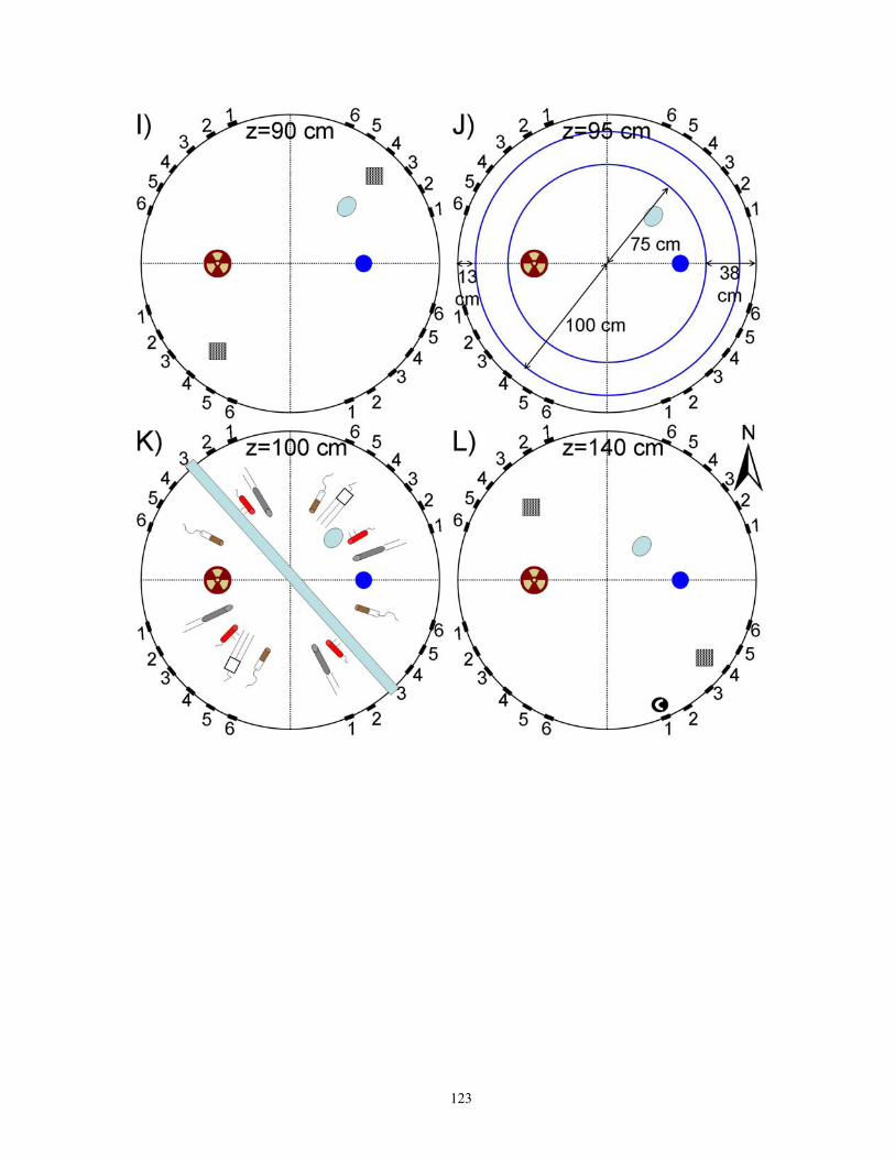
123

124

125

Figure C-1. A) Lysimeter dimensions, porthole numbers, and quadrants. Instrument map

for lysimeters at depth B) 0 cm; C) 5 cm; D); 10 cm; E) 25 cm; F) 50 cm; G) 60 cm; H) 75 cm; I) 90 cm; J) 95 cm; K) 100 cm; L) 140 cm; M) 150 cm; N) 190 cm; O) 200 cm; P) 250 cm; and Q) 295 cm. R) Depth profile for the placement of Heat Flux Plates and TCAVS at 2, 6, and 8 cm depth.

126

Table C-1. Serial number, placement, and datalogger variable ID of DPHP in lysimeters 1, 2, and 3.

Serial Number Placement Porthole WXY1Y2Z1Z2

Heater Board

1653 R1_D250_NE R1_NE2_D250 111402 HB IV 1655 R1_D250_SW R1_SW2_D250 131402 HB IV 1656 R1_D200_SE R1_SE4_D150 121302 HB VI 1658 R1_D200_NW R1_NW4_D150 141302 HB IV 1659 R1_D150_NE R1_NE4_D150 111102 HB VII 1660 R1_D150_SE R1_SE4_D150 121102 HB VII 1661 R1_D150_SW R1_SW4_D150 131102 HB VI 1662 R1_D150_NW R1_NW4_D150 141102 HB VI 1664 R1_D100_NE R1_NE2_D150 110902 HB VII 1665 R1_D100_SE R1_SE2_D150 120902 HB VII 1666 R1_D100_SW R1_SW2_D150 130902 HB VII 1667 R1_D100_NW R1_NW2_D150 140902 HB VI 1668 R1_D75_NW R1_NE4_D100 110702 HB IV 1669 R1_D75_SE R1_SE4_D100 120702 HB V 1670 R1_D75_SW R1_SW4_D100 130702 HB V 1671 R1_D75_NW R1_NW4_D100 140702 HB V 1672 R1_D50_NE R1_NE6_D80 110502 HB I 1673 R1_D50_SE R1_SE6_D80 120502 HB V 1674 R1_D50_SW R1_SW6_D80 130502 HB IV 1675 R1_D50_NW R1_NW6_D80 140502 HB IV 1676 R1_D25_SE R1_SE2_D80 120402 HB I 1677 R1_D25_NW R1_NW2_D80 140402 HB I 1679 R1_D10_SE R1_SE3_D80 120302 HB I 1680 R1_D10_NW R1_NW3_D80 140302 HB I 1682 R2_D250_NE R2_NE2_D250 211402 1683 R2_D250_SW R2_SW2_D250 231402 1684 R2_D200_SE R2_SE4_D150 221302 1685 R2_D200_NW R2_NW4_D150 241302 1681 R2_D150_NE R2_NE4_D150 211102 1686 R2_D150_SE R2_SE4_D150 221102 1687 R2_D150_SW R2_SW4_D150 231102 1688 R2_D150_NW R2_NW4_D150 241102 1689 R2_D100_NE R2_NE2_D150 210902 1690 R2_D100_SE R2_SE2_D150 220902 1691 R2_D100_SW R2_SW2_D150 230902 1692 R2_D100_NW R2_NW2_D150 240902

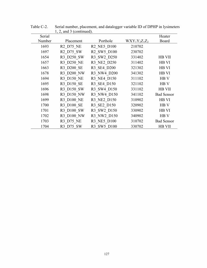
127

Table C-2. Serial number, placement, and datalogger variable ID of DPHP in lysimeters 1, 2, and 3 (continued).

Serial Number Placement Porthole WXY1Y2Z1Z2

Heater Board

1693 R2_D75_NE R2_NE5_D100 210702 1697 R2_D75_SW R2_SW5_D100 230702 1654 R3_D250_SW R3_SW2_D250 331402 HB VII 1657 R3_D250_NE R3_NE2_D250 311402 HB VI 1663 R3_D200_SE R3_SE4_D200 321302 HB VI 1678 R3_D200_NW R3_NW4_D200 341302 HB VI 1694 R3_D150_NE R3_NE4_D150 311102 HB V 1695 R3_D150_SE R3_SE4_D150 321102 HB V 1696 R3_D150_SW R3_SW4_D150 331102 HB VII 1698 R3_D150_NW R3_NW4_D150 341102 Bad Sensor 1699 R3_D100_NE R3_NE2_D150 310902 HB VI 1700 R3_D100_SE R3_SE2_D150 320902 HB V 1701 R3_D100_SW R3_SW2_D150 330902 HB VI 1702 R3_D100_NW R3_NW2_D150 340902 HB V 1703 R3_D75_NE R3_NE5_D100 310702 Bad Sensor 1704 R3_D75_SW R3_SW5_D100 330702 HB VII

128

Table C-3. Serial number, placement, and datalogger variable ID of Heat Dissipating Units (HDUs) in lysimeters 1, 2 and 3.

Serial Number Placement Porthole WXY1Y2Z1Z2 12260 R1_D250_NE R1_NE5_D250 111404 12261 R1_D250_SW R1_SW5_D250 131404 12262 R1_D200_SE R1_SE6_D150 121304 12263 R1_D200_NW R1_NW6_D150 141304 12264 R1_D150_NE R1_NE6_D150 111104 12265 R1_D150_SE R1_SE6_D150 121104 12266 R1_D150_SW R1_SW6_D150 131104 12267 R1_D150_NW R1_NW6_D150 141104 12268 R1_D100_NE R1_NE2_D150 110904 12269 R1_D100_SE R1_SE2_D150 120904 12270 R1_D100_SW R1_SW2_D150 130904 12271 R1_D100_NW R1_NW2_D150 140904 12272 R1_D75_NE R1_NE6_D100 110704 12273 R1_D75_SE R1_SE6_D100 120704 12274 R1_D75_SW R1_SW6_D100 130704 12259 R1_D75_NW R1_NW6_D100 140704 12276 R1_D50_NE R1_NE6_D80 110504 12277 R1_D50_SE R1_SE6_D80 120504 12278 R1_D50_SW R1_SW6_D80 130504 12279 R1_D50_NW R1_NW6_D80 140504 12280 R1_D25_NE R1_NE2_D80 110404 12281 R1_D25_SE R1_SE2_D80 120404 12282 R1_D25_SW R1_SW2_D80 130404 12283 R1_D25_NW R1_NW2_D80 140404 12284 R1_D10_NE R1_NE3_D80 110304 12285 R1_D10_SE R1_SE3_D80 120304 12286 R1_D10_SW R1_SW3_D80 130304 12287 R1_D10_NW R1_NW3_D80 140304 12288 R1_D5_NE R1_NE5_D60 110204 12289 R1_D5_SE R1_SE5_D60 120204 12320 R1_D5_SW R1_SW5_D60 130204 12321 R1_D5_NW R1_NW5_D60 140204 12322 R2_D250_SW R2_SW5_D250 231404 12323 R2_D250_NE R2_NE5_D250 211404 12324 R2_D200_SE R2_SE6_D150 221304 12325 R2_D200_NW R2_NW6_D150 241304 12326 R2_D150_NE R2_NE6_D150 211104 12327 R2_D150_SE R2_SE6_D150 221104 12328 R2_D150_SW R2_SW6_D150 231104 12329 R2_D150_NW R2_NW6_D150 241104 12330 R2_D100_NE R2_NE2_D150 210904

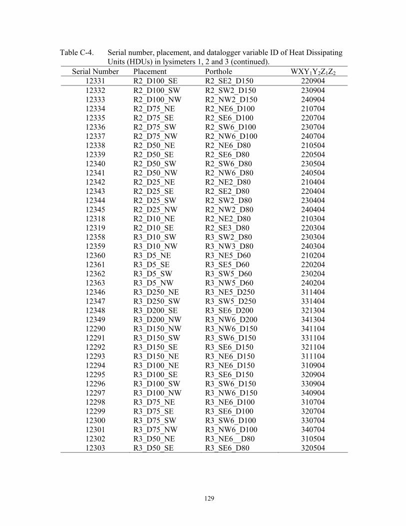
129

Table C-4. Serial number, placement, and datalogger variable ID of Heat Dissipating Units (HDUs) in lysimeters 1, 2 and 3 (continued).

Serial Number Placement Porthole WXY1Y2Z1Z2 12331 R2_D100_SE R2_SE2_D150 220904 12332 R2_D100_SW R2_SW2_D150 230904 12333 R2_D100_NW R2_NW2_D150 240904 12334 R2_D75_NE R2_NE6_D100 210704 12335 R2_D75_SE R2_SE6_D100 220704 12336 R2_D75_SW R2_SW6_D100 230704 12337 R2_D75_NW R2_NW6_D100 240704 12338 R2_D50_NE R2_NE6_D80 210504 12339 R2_D50_SE R2_SE6_D80 220504 12340 R2_D50_SW R2_SW6_D80 230504 12341 R2_D50_NW R2_NW6_D80 240504 12342 R2_D25_NE R2_NE2_D80 210404 12343 R2_D25_SE R2_SE2_D80 220404 12344 R2_D25_SW R2_SW2_D80 230404 12345 R2_D25_NW R2_NW2_D80 240404 12318 R2_D10_NE R2_NE2_D80 210304 12319 R2_D10_SE R2_SE3_D80 220304 12358 R3_D10_SW R3_SW2_D80 230304 12359 R3_D10_NW R3_NW3_D80 240304 12360 R3_D5_NE R3_NE5_D60 210204 12361 R3_D5_SE R3_SE5_D60 220204 12362 R3_D5_SW R3_SW5_D60 230204 12363 R3_D5_NW R3_NW5_D60 240204 12346 R3_D250_NE R3_NE5_D250 311404 12347 R3_D250_SW R3_SW5_D250 331404 12348 R3_D200_SE R3_SE6_D200 321304 12349 R3_D200_NW R3_NW6_D200 341304 12290 R3_D150_NW R3_NW6_D150 341104 12291 R3_D150_SW R3_SW6_D150 331104 12292 R3_D150_SE R3_SE6_D150 321104 12293 R3_D150_NE R3_NE6_D150 311104 12294 R3_D100_NE R3_NE6_D150 310904 12295 R3_D100_SE R3_SE6_D150 320904 12296 R3_D100_SW R3_SW6_D150 330904 12297 R3_D100_NW R3_NW6_D150 340904 12298 R3_D75_NE R3_NE6_D100 310704 12299 R3_D75_SE R3_SE6_D100 320704 12300 R3_D75_SW R3_SW6_D100 330704 12301 R3_D75_NW R3_NW6_D100 340704 12302 R3_D50_NE R3_NE6__D80 310504 12303 R3_D50_SE R3_SE6_D80 320504

130

Table C-5. Serial number, placement, and datalogger variable ID of Heat Dissipating Units (HDUs) in lysimeters 1, 2 and 3 (continued).

Serial Number Placement Porthole WXY1Y2Z1Z2 12304 R3_D50_SW R3_SW6_D80 330504 12305 R3_D50_NW R3_NW6_D80 340504 12306 R3_D25_NE R3_NE6_D80 310404 12307 R3_D25_SE R3_SE6_D80 320404 12308 R3_D25_SW R3_SW6_D80 330404 12309 R3_D25_NW R3_NW6_D80 340404 12310 R3_D10_NE R3_NE2_D80 310304 12311 R3_D10_SE R3_SE3_D80 320304 12312 R3_D10_SW R3_SW2_D80 330304 12313 R3_D10_NW R3_NW3_D80 340304 12314 R3_D5_NE R3_NE5_D60 310204 12315 R3_D5_SE R3_SE5_D60 320204 12316 R3_D5_SW R3_SW5_D60 330204 12317 R3_D5_NW R3_NW5_D60 340204

131

Table C-6. Serial number, placement, and datalogger variable ID of settlement plates in lysimeters 1, 2, and 3.

Serial Number Placement Porthole WXY1Y2Z1Z2 1 R1_D190_NE R1_NE3_D150 111210 2 R1_D190_SW R1_SW3_D150 131210 3 R1_D140_NW R1_NW2_D100 141010 4 R1_D140_SE R1_SE2_D100 121010 5 R1_D90_NE R1_NE2_D60 110810 6 R1_D90_SW R1_SW2_D60 130810 7 R2_D190_NE R2_NE3_D150 211210 8 R2_D190_SW R2_SW3_D150 231210 9 R2_D140_NW R2_NW2_D100 241010 10 R2_D140_SE R2_SE2_D100 221010 11 R2_D90_NE R2_NE2_D60 210810 12 R2_D90_SW R2_SW2_D60 230810 13 R3_D190_NE R3_NE3_D150 311210 14 R3_D190_SW R3_SW3_D150 331210 15 R3_D140_NW R3_NW2_D100 341010 16 R3_D140_SE R3_SE2_D100 321010 17 R3_D90_NE R3_NE2_D60 310810 18 R3_D90_SW R3_SW2_D60 330810

132

Table C-7. Serial number, placement, and datalogger variable ID of SSS in lysimeters 1, 2, and 3.

Serial Number Placement Porthole WXY1Y2Z1Z2 L3 R1_D295_SW R1_NW3_D295 131505 L14 R1_D295_N R1_NW1_D295 151505 L15 R1_D295_NW R1_NW2_D295 141505 L16 R1_D295_SE R1_SE2_D295 121505 L17 R1_D295_S R1_SE1_D295 171505 L20 R1_D295_NE R1_SE2_D295 111505 S25 R1_D250_NE R1_NE1_D250 111405 S26 R1_D250_SW R1_SW1_D250 131405 S27 R1_D200_SE R1_SE1_D150 121305 S28 R1_D200_NW R1_NW1_D150 141305 S21 R1_D150_NE R1_NE1_D150 111105 S22 R1_D150_SE R1_SE1_D150 121105 S23 R1_D150_SW R1_SW1_D150 131105 S24 R1_D150_NW R1_NW1_D150 141105 S20 R1_D100_NE R1_NE1_D100 110905 S19 R1_D100_SE R1_SE1_D100 120905 S15 R1_D100_SW R1_SW1_D100 130905 S14 R1_D100_NW R1_NW1_D100 140905 S13 R1_D75_NE R1_NE5_D80 110705 S12 R1_D75_SE R1_SE5_D80 120705 S11 R1_D75_SW R1_SW5_D80 130705 S10 R1_D75_NW R1_NW5_D80 140705 S09 R1_D50_NE R1_NE1_D60 110505 S08 R1_D50_SE R1_SE1_D60 120505 S06 R1_D50_SW R1_SW1_D60 130505 S01 R1_D50_NW R1_NW1_D60 140505 L01 R2_D295_N R2_NW1_D295 231505 L02 R2_D295_NE R2_SE2_D295 251505 L04 R2_D295_SE R2_SE2_D295 241505 L05 R2_D295_S R2_SE1_D295 221505 L06 R2_D295_SW R2_NW3_D295 271505 L07 R2_D295_NW R2_NW2_D295 211505 S32 R2_D250_NE R2_NE1_D250 211405 S33 R2_D250_SW R2_SW1_D250 231405 S35 R2_D200_SE R2_SE1_D150 221305 S36 R2_D200_NW R2_NW1_D150 241305 S4 R2_D150_NE R2_NE1_D150 211105 S5 R2_D150_SE R2_SE1_D150 221105 S31 R2_D150_SW R2_SW1_D150 231105 S38 R2_D150_NW R2_NW1_D150 241105 S2 R2_D100_NE R2_NE1_D100 210905 S3 R2_D100_SE R2_SE1_D100 220905

133

Table C-8. Serial number, placement, and datalogger variable ID of SSS in lysimeters 1, 2, and 3 (continued).

Serial Number Placement Porthole WXY1Y2Z1Z2 S7 R2_D100_SW R2_SW1_D100 230905 S17 R2_D100_NW R2_NW1_D100 240905 S29 R2_D75_NE R2_NE5_D80 210705 S34 R2_D75_SE R2_SE5_D80 220705 S37 R2_D75_SW R2_SW5_D80 230705 S39 R2_D75_NW R2_NW5_D80 240705

S29A R2_D50_NE R2_NE1_D60 210505 S40 R2_D50_SE R2_SE1_D60 220505 S41 R2_D50_SW R2_SW1_D60 230505 S42 R2_D50_NW R2_NW1_D60 240505 L08 R3_D295_N R3_SE3_D295 331505 L09 R3_D295_NE R3_SE3_D295 351505 L10 R3_D295_SE R3_SE2_D295 341505 L11 R3_D295_S R3_SE2_D295 321505 L12 R3_D295_SW R3_SE1_D295 371505 L13 R3_D295_NE R3_NW3_D295 311505 S44 R3_D250_NE R3_NE1_D250 311405 S45 R3_D250_SW R3_SW1_D250 331405 S46 R3_D200_SE R3_SE1_D200 321305 S47 R3_D200_NW R3_NW1_D200 341305 S48 R3_D150_NE R3_NE1_D150 311105 S49 R3_D150_SE R3_SE1_D150 321105 S50 R3_D150_SW R3_SW1_D150 331105 S51 R3_D150_NW R3_NW1_D150 341105 S52 R3_D100_NE R3_NE1_D100 310905 S53 R3_D100_SE R3_SE1_D100 320905 S54 R3_D100_SW R3_SW1_D100 330905 S55 R3_D100_NW R3_NW1_D100 340905 S56 R3_D75_NE R3_NE5_D80 310705 S57 R3_D75_SE R3_SE5_D80 320705 S58 R3_D75_SW R3_SW5_D80 330705 S59 R3_D75_NW R3_NW5_D80 340705 S60 R3_D50_NE R3_NE1_D60 310505 S61 R3_D50_SE R3_SE1_D60 320505 S62 R3_D50_SW R3_SW1_D60 330505 S63 R3_D50_NW R3_NW1_D60 340505

134

Table C-9. Serial number, placement, and datalogger variable ID of TPHPs in lysimeters 1, 2, and 3.

Serial Number Placement Porthole WXY1Y2Z1Z2 Heater Board

1708 R1_D25_NE R1_NE2_D80 110403 HB II 1709 R1_D25_SW R1_SW2_D80 130403 HB II 1710 R1_D10_NE R1_NE3_D80 120303 HB II 1711 R1_D10_SW R1_SW3_D80 140303 HB II 1712 R1_D5_SE R1_SE2_D60 120203 HB III 1713 R1_D5_SE R1_SE2_D60 120203 HB III 1714 R1_D5_SE R1_SE2_D60 120203 HB III 1715 R1_D5_SE R1_SE2_D60 120203 HB III 1716 R2_D75_SE R2_SE5_D100 220703 1717 R2_D75_NW R2_NW5_D100 240703 1718 R2_D50_NE R2_NE3_D80 210503 1719 R2_D50_SE R2_SE3_D80 220503 1720 R2_D50_SW R2_SW3_D80 230503 1721 R2_D50_NW R2_NW3_D80 240503 1722 R2_D25_NE R2_NE2_D80 210403 1723 R2_D25_SE R2_SE2_D80 220403 1724 R2_D25_SW R2_SW2_D80 230403 1725 R2_D25_NW R2_NW2_D80 240403 1726 R2_D10_NE R2_NE3_D80 210303 1727 R2_D10_SE R2_SE2_D80 220303 1728 R2_D10_SW R2_SW3_D80 230303 1729 R2_D10_NW R2_NW2_D80 240303 1730 R2_D5_SE R2_SE2_D80 220203 1731 R2_D5_SE R2_SE2_D80 220203 1732 R2_D5_SE R2_SE2_D80 220203 1733 R2_D5_SE R2_SE2_D80 220203 1734 R3_D75_SE R3_SE5_D100 320703 HB III 1735 R3_D75_NW R3_NW5_D100 340703 HB II 1736 R3_D50_NE R3_NE3_D80 310503 HB II 1737 R3_D50_SE R3_SE3_D80 320503 HB III 1738 R3_D50_SW R3_SW3_D80 330503 HB I 1739 R3_D50_NW R3_NW3_D80 340503 HB I 1740 R3_D25_NE R3_NE2_D80 310403 HB I 1741 R3_D25_SE R3_SE2_D80 320403 HB II 1742 R3_D25_SW R3_SW2_D80 330403 HB IV 1743 R3_D25_NW R3_NW2_D80 340403 HB III 1744 R3_D10_NE R3_NE3_D80 310303 HB II

135

Table C-10. Serial number, placement, and datalogger variable ID of TPHPs in lysimeters 1, 2, and 3 (continued).

Serial Number Placement Porthole WXY1Y2Z1Z2 Heater Board

1745 R3_D10_SE R3_SE2_D80 320303 HB IV 1746 R3_D10_SW R3_SW3_D80 330303 HB I 1747 R3_D10_NW R3_NW2_D80 340303 HB II 1748 R3_D5_SE R3_SE2_D60 320203 HB IV 1749 R3_D5_SE R3_SE2_D60 320203 HB III 1754 R3_D5_SE R3_SE2_D60 320203 HB IV 1751 R3_D5_SE R3_SE2_D60 320203 HB IV

136

Table C-11. Serial number, placement, and datalogger variable ID of TDRs in lysimeters 1, 2, and 3.

Serial Number Placement Porthole WXY1Y2Z1Z2 SDMX50 port TDR100

1 R1_D250_NE R1_NE4_D250 111401 4824 8 2018 2 R1_D250_SW R1_SW4_D250 131401 4824 7 2018 3 R1_D200_SE R1_SE5_D150 121301 4824 6 2018 4 R1_D200_NW R1_NW5_D150 141301 4824 5 2018 5 R1_D150_NE R1_NE5_D150 111101 4824 4 2018 6 R1_D150_SE R1_SE5_D150 121101 4824 3 2018 7 R1_D150_SW R1_SW5_D150 131101 4824 2 2018 8 R1_D150_NW R1_NW5_D150 141101 4824 1 2018 9 R1_D100_NE R1_NE3__D100 110901 4823 8 2018 10 R1_D100_SW R1_SW3_D100 130901 4823 7 2018 11 R1_D75_NE R1_NE5_D100 110701 4823 6 2018 12 R1_D75_SE R1_SE5_D100 120701 4823 5 2018 13 R1_D75_SW R1_SW5_D100 130701 4823 4 2018 14 R1_D75_NW R1_NW5_D100 140701 4823 3 2018 15 R1_D50_NE R1_NE4_D80 110501 4823 2 2018 16 R1_D50_SE R1_SE4_D80 120501 4823 1 2018 17 R1_D50_SW R1_SW4_D80 130501 4821 8 2018 18 R1_D50_NW R1_NW4_D80 140501 4821 7 2018 19 R1_D25_NE R1_NE1_D80 110401 4821 6 2018 20 R1_D25_SE R1_SE1_D80 120401 4821 5 2018 21 R1_D25_SW R1_SW1_D80 130401 4821 4 2018 22 R1_D25_NW R1_NW1_D80 140401 4821 3 2018 23 R1_D10_NE R1_NE4_D60 110301 4821 2 2018 24 R1_D10_SE R1_SE4_D60 120301 4821 1 2018 25 R1_D10_SW R1_SW4_D60 130301 4822 2 2018 26 R1_D10_NW R1_NW4_D60 140301 4822 1 2018 27 R2_D250_NE R2_NE4_D250 211401 4868 8 2019 28 R2_D250_SW R2_SW4_D250 231401 4868 7 2019 29 R2_D200_SE R2_SE5_D150 221301 4868 6 2019 30 R2_D200_NW R2_NW5_D150 241301 4868 5 2019 32 R2_D150_NE R2_NE5_D150 211101 4868 4 2019 33 R2_D150_SE R2_SE5_D150 221101 4868 3 2019 34 R2_D150_SW R2_SW5_D150 231101 4868 2 2019 35 R2_D150_NW R2_NW5_D150 241101 4868 1 2019 36 R2_D100_NE R2_NE3_D100 210901 4869 8 2019 37 R2_D100_SW R2_SW3_D100 230901 4869 7 2019 38 R2_D75_NE R2_NE4_D100 210701 4869 6 2019 39 R2_D75_SE R2_SE4_D100 220701 4869 5 2019 40 R2_D75_SW R2_SW4_D100 230701 4869 4 2019 41 R2_D75_NW R2_NW4_D100 240701 4869 3 2019 42 R2_D50_NE R2_NE4_D80 210501 4869 2 2019

137

Table C-12. Serial number, placement, and datalogger variable ID of TDRs in lysimeters 1, 2, and 3 (continued).

Serial Number Placement Porthole WXY1Y2Z1Z2 SDMX50 port TDR100

43 R2_D50_SE R2_SE4_D80 220501 4869 1 2019 44 R2_D50_SW R2_SW4_D80 230501 4814 8 2019 45 R2_D50_NW R2_NW4_D80 240501 4814 7 2019 46 R2_D25_NE R2_NE1_D80 210401 4814 6 2019 47 R2_D25_SE R2_SE1_D80 220401 4814 5 2019 48 R2_D25_SW R2_SW1_D80 230401 4814 4 2019 49 R2_D25_NW R2_NW1_D80 240401 4814 3 2019 60 R2_D10_NE R2_NE4_D60 210301 4814 2 2019 61 R2_D10_SE R2_SE4_D60 220301 4814 1 2019 62 R2_D10_SW R2_SW4_D60 230301 4818 2 2019 63 R2_D10_NW R2_NW4_D60 240301 4818 1 2019 53 R3_D250_NE R3_NE4_D250 311401 4819 8 2090 54 R3_D250_SW R3_SW4_D250 331401 4819 7 2090 55 R3_D200_SE R3_SE5_D200 321301 4819 6 2090 56 R3_D200_NW R3_NW5_D200 341301 4819 5 2090 50 R3_D150_NE R3_NE5_D150 311101 4819 4 2090 51 R3_D150_SE R3_SE5_D150 321101 4819 3 2090 52 R3_D150_SW R3_SW5_D150 331101 4819 2 2090 57 R3_D150_NW R3_NW5_D150 341101 4819 1 2090 58 R3_D100_NE R3_NE3_D100 310901 4820 8 2090 59 R3_D100_SW R3_SW3_D100 330901 4820 7 2090 68 R3_D75_NE R3_NE4_D100 310701 4820 6 2090 69 R3_D75_SE R3_SE4_D100 320701 4820 5 2090 70 R3_D75_SW R3_SW4_D100 330701 4820 4 2090 71 R3_D75_NW R3_NW4_D100 340701 4820 3 2090 72 R3_D50_NE R3_NE4_D80 310501 4820 2 2090 73 R3_D50_SE R3_SE4_D80 320501 4820 1 2090 74 R3_D50_SW R3_SW4_D80 330501 4989 8 2090 75 R3_D50_NW R3_NW4_D80 340501 4989 7 2090 76 R3_D25_NE R3_NE1_D80 310401 4989 6 2090 77 R3_D25_SE R3_SE1_D80 320401 4989 5 2090 78 R3_D25_SW R3_SW1_D80 330401 4989 4 2090 79 R3_D25_NW R3_NW1_D80 340401 4989 3 2090 80 R3_D10_NE R3_NE4_D60 310301 4989 2 2090 81 R3_D10_SE R3_SE4_D60 320301 4989 1 2090 83 R3_D10_SW R3_SW4_D60 330301 4867 2 2090 84 R3_D10_NW R3_NW4_D60 340301 4867 1 2090

138

Table C-13. Serial number, placement, and datalogger variable ID of 108L in lysimeters 1, 2, and 3.

Serial Number Placement Porthole WXY1Y2Z1Z2 1 R1_D75_E R1_SE6_D60 160706 2 R1_D50_E R1_SE6_D60 160506 3 R1_D25_E R1_NE6_D60 160406 4 R1_D5_E R1_NE6_D60 160206 5 R2_D75_E R2_SE6_D60 260706 6 R2_D50_E R2_SE6_D60 260506 7 R2_D25_E R2_NE6_D60 260406 12 R2_D5_E R2_NE6_D60 260206 8 R3_D75_E R3_SE6_D60 360706 9 R3_D50_E R3_SE6_D60 360506 10 R3_D25_E R3_NE6_D60 360406 11 R3_D5_E R3_NE6_D60 360206

Table C-14. Serial number, placement, and datalogger variable ID of ECH2O-TE in

lysimeters 1, 2, and 3. Serial Number Placement Porthole WXY1Y2Z1Z2

1 R1_D5_NE R1_NE6_D60 110209 2 R1_D5_SW R1_SW6_D60 130209 5 R2_D5_NE R2_NE6_D60 210209 6 R2_D5_SW R2_SW6_D60 230209 3 R3_D5_NE R3_NE6_D60 310209 4 R3_D5_SW R3_SW6_D60 330209

Table C-15. Serial number, placement, and datalogger variable ID of heat flux plates in

lysimeters 1, 2, and 3. Serial Number Placement Porthole WXY1Y2Z1Z2

1173 R1_D5_NE R1_SE5_D60 110207 1180 R1_D5_SW R1_SW3_D60 130207 1190 R2_D5_NE R2_SE5_D60 210207 1193 R2_D5_SW R2_SW3_D60 230207 1174 R3_D5_NE R3_SE5_D60 310207 1181 R3_D5_SW R3_SW3_D60 330207

Table C-16. Serial number, placement, and datalogger variable ID of TCAVs in lysimeters

1, 2, and 3. Serial Number Placement Porthole WXY1Y2Z1Z2

1 R1_D5_SE R1_SE5_D60 120208 2 R2_D5_SE R2_SE5_D60 220208 3 R3_D5_SE R3_SE5_D60 320208

139

Table C-17. Serial number, placement, and datalogger variable ID of FDR (CS616) in lysimeters 1, 2, and 3.

Serial Number Placement Porthole WXY1Y2Z1Z2 NA R1_D5_SW R1_SW3_D60 130214

140


141

APPENDIX D. TRACERS

Table D-1. Parameters to determine tracer volume and mass need for lysimeter application*.

Name Variable Value Unit Formula Diameter D 2.258 m - Surface area Lysimeter A 4.00 m2 0.25*PI()*D^2 Height of Lysimeter H 3.00 m - Volume of lysimeter V 12.01 m3 A*H Expected bulk density Pb 1.60 Mg m-3 - Porosity N 0.396 1-pb/2.65 Expect pore volume PV 4.760 m3 V*n *Assumptions: 1. Tracer is uniformly mixed throughout the lysimeter 2. Water is uniformly mixed throughout lysimeter 3. 1 m3 is equal to 1000 L

Table D-2. Volume of water in lysimeter at specific water content (in liters).

θv Vol of H2O [m3/m3] [L]

0.05 600.66 0.10 1201.32 0.15 1801.98 0.20 2402.64 0.25 3003.30 0.30 3603.96 0.35 4204.62 0.40 4805.28

142

Table D-3. Tracer mass needed (in g) for different water contents.** θv Br

[m3/m3] [g] 0.05 3.00 0.10 6.01 0.15 9.01 0.20 12.01 0.25 15.02 0.30 18.02 0.35 21.02 0.40 24.03

**Assume minimum detection of 5 mg/L. Table D-4. Amount of CaBr need at different water contents.***

θv CaBr [m3/m3] [g]

0.05 3.75 0.10 7.51 0.15 11.26 0.20 15.02 0.25 18.77 0.30 22.52 0.35 26.28

***CaBr is equal to 0.8 Br. Table D-5. Determining volume of CaBr mixture for each mesh square using 2 pipettes

for the total application of 15.02 g of CaBr for 12.01 g of Br mixed in 1000 L of water.

Parameter Value Unit Formula Length of Remesh 0.15 m L Area of Remesh openings 0.0225 m2 L^2 # of Squares 178 Squares A/L^2 Volume of CaBr 1000 mL - Volume of CaBr/Square 5.619 CaBr/square Vol of CaBr/# of squares 2 pipettes 2 pipettes -

Volume per pipette 2.809 mL/pipette Vol of CaBr/# of squares/2 pipettes

143

Table D-6. Mass of CaBr mixed with 1000 L of water.

Lysimeter Mass of

CaBr Vol. of Water Mixed by Applied by

[g] [L]

1 15.01 1000 Todd Arrowood Todd Arrowood

2 12.01 1000 Karletta Chief Beth Johnson

3 12.01 1000 Jarai Mon Graduate students

Note: Each mixture was mixed for 10-15 minutes until there is no cloudiness or crystals. There was a mistake of applying 12.01 g of CaBr on lysimeter 2. Since lysimeter 2 and 3 are replicates, 12.01 g of CaBr was also applied on lysimeter 3. Error will not be significant and Br will still be detected in 1 pore volume.

144


145

APPENDIX E. HDU AND TDR CALIBRATION PARAMETERS

Table E-1. HDU serial numbers and Bilskie fitting parameters. Serial Number del_Tdry1 del_Twet1 Alpha beta

12259 2.6506 0.6991 129.9230 0.2592 12260 2.9190 0.7281 129.9230 0.3272 12261 2.8695 0.7068 129.9230 0.2875 12262 2.8127 0.7307 129.9230 0.3038 12263 2.8604 0.7244 129.9230 0.2794 12264 2.7746 0.7201 129.9230 0.2627 12265 2.8802 0.7077 129.9230 0.2882 12266 2.8548 0.7276 129.9230 0.2543 12267 2.8271 0.7309 129.9230 0.2568 12268 2.8180 0.7243 129.9230 0.2678 12269 2.7919 0.7506 129.9230 0.2613 12270 2.9064 0.7133 129.9230 0.2590 12271 2.8039 0.6985 129.9230 0.2625 12272 2.7358 0.6936 129.9230 0.2691 12273 2.7998 0.6837 129.9230 0.2679 12274 2.7455 0.7073 129.9230 0.2831 12276 2.8528 0.6967 129.9230 0.2971 12277 2.8000 0.7087 129.9230 0.2929 12278 2.7591 0.7020 129.9230 0.2935 12279 2.8096 0.7187 129.9230 0.2923 12280 2.7532 0.7094 129.9230 0.2889 12281 2.8666 0.6968 129.9230 0.2961 12282 3.1201 0.7508 129.9230 0.3037 12283 2.7284 0.7040 129.9230 0.2520 12284 2.8197 0.7090 129.9230 0.2591 12285 2.8881 0.7032 129.9230 0.2432 12286 3.0012 0.6855 129.9230 0.2932 12287 2.8666 0.6966 129.9230 0.2691 12288 2.5988 0.7037 129.9230 0.2515 12289 2.7046 0.7038 129.9230 0.2656 12290 2.8933 0.7291 157.1681 0.3103 12291 2.8463 0.7378 157.1681 0.3110 12292 2.8604 0.7317 157.1681 0.3157 12293 2.8169 0.7193 157.1681 0.3285 12294 2.8117 0.7245 157.1681 0.3027 12295 2.7389 0.7212 157.1681 0.2712 12296 2.7268 0.7586 157.1681 0.2648

146

Table E-2. HDU serial numbers and Bilskie fitting parameters (continued). Serial Number del_Tdry1 del_Twet1 Alpha beta

12297 2.8018 0.7474 157.1681 0.2650 12298 2.7446 0.7676 157.1681 0.2703 12299 2.8988 0.7601 157.1681 0.2752 12300 3.0017 0.7540 157.1681 0.2929 12301 2.8560 0.6949 157.1681 0.2743 12302 2.7731 0.7282 157.1681 0.2436 12303 2.8904 0.7303 157.1681 0.3009 12304 2.7781 0.7428 157.1681 0.3024 12305 2.7951 0.7233 157.1681 0.3031 12306 2.8334 0.7230 157.1681 0.2841 12307 2.5846 0.7048 157.1681 0.2852 12308 2.8439 0.7194 157.1681 0.2726 12309 2.7869 0.7271 157.1681 0.2876 12310 2.8644 0.6855 157.1681 0.2635 12311 2.6145 0.6881 157.1681 0.2684 12312 2.8764 0.6983 157.1681 0.3001 12313 2.7226 0.6870 157.1681 0.2596 12314 2.7762 0.6750 157.1681 0.2964 12315 2.8477 0.7401 157.1681 0.3164 12316 2.6156 0.6732 157.1681 0.2828 12317 2.6740 0.6544 157.1681 0.2869 12318 2.7290 0.4488 157.1681 0.2725 12319 2.7328 0.6423 157.1681 0.3114 12320 2.8209 0.8103 114.2434 0.3184 12321 2.8044 0.7716 114.2434 0.3006 12322 2.8122 0.7371 114.2434 0.2980 12323 2.7451 0.7516 114.2434 0.2664 12324 2.8175 0.7629 114.2434 0.2445 12325 2.9226 0.7844 114.2434 0.2736 12326 2.7728 0.7266 114.2434 0.2599 12327 2.9808 0.8086 114.2434 0.2681 12328 2.9681 0.7495 114.2434 0.2597 12329 2.9188 0.7770 114.2434 0.2926 12330 2.8813 0.7616 114.2434 0.2590 12331 2.7820 0.6838 114.2434 0.2895 12332 2.8470 0.7243 114.2434 0.3087 12333 2.8584 0.7606 114.2434 0.3304 12334 2.8058 0.7252 114.2434 0.3465

147


12335 2.7716 0.6578 114.2434 0.3448 12336 2.7264 0.6420 114.2434 0.3196 12337 2.6349 0.6260 114.2434 0.3187 12338 2.8597 0.6602 114.2434 0.3426 12339 2.9506 0.6555 114.2434 0.3273 12340 2.8461 0.6527 114.2434 0.3030 12341 2.7335 0.6695 114.2434 0.2778 12342 2.6696 0.6687 114.2434 0.2592 12343 2.7066 0.6450 114.2434 0.2537 12344 2.7507 0.6555 114.2434 0.2609 12345 2.6012 0.6422 114.2434 0.2370 12346 2.7340 0.6215 114.2434 0.2704 12347 2.7665 0.6341 114.2434 0.2948 12348 2.5837 0.6273 114.2434 0.2946 12349 2.6339 0.6439 114.2434 0.2731 12358 2.8554 0.7786 130.6061 0.2511 12359 2.5918 0.7223 130.6061 0.2470 12360 2.7895 0.7366 130.6061 0.2499 12361 2.8695 0.7584 130.6061 0.2628 12362 2.8311 0.7641 130.6061 0.2608 12363 2.6512 0.7429 130.6061 0.2436 12364 2.7586 0.7509 130.6061 0.2409 12365 2.8786 0.7303 130.6061 0.2571 12366 2.7372 0.7354 130.6061 0.2538 12367 2.7151 0.7292 130.6061 0.2450 12368 2.8054 0.7492 130.6061 0.2493 12369 2.8016 0.7294 130.6061 0.2138 12370 2.7387 0.6689 130.6061 0.2404 12371 2.6040 0.7261 130.6061 0.2673 12372 2.8661 0.7020 130.6061 0.3290 12373 3.1128 0.7442 130.6061 0.2173 12616 2.7188 0.7982 134.6838 0.3747 12617 2.8599 0.8361 134.6838 0.3865 12618 2.7489 0.8145 134.6838 0.4062 12619 2.7172 0.8139 134.6838 0.3832 12620 2.8459 0.8324 134.6838 0.3801 12621 2.8440 0.7899 134.6838 0.3935 12622 2.7820 0.7882 134.6838 0.3677

148


12623 2.8489 0.8089 134.6838 0.3594 12624 2.8355 0.8073 134.6838 0.3971 12625 2.7957 0.7881 134.6838 0.3771 12626 2.8824 0.8113 134.6838 0.3875 12627 2.6975 0.7052 134.6838 0.4036 12628 2.8456 0.7862 134.6838 0.3918 12629 2.8879 0.8410 134.6838 0.3887 12630 2.7657 0.7925 134.6838 0.3807 12631 2.9068 0.8453 134.6838 0.4126 12632 2.5384 0.6072 134.6838 0.3797 12633 2.8568 0.7988 134.6838 0.3745 12634 2.8013 0.8059 134.6838 0.3977 12635 2.7373 0.8042 134.6838 0.4090 12636 2.8119 0.7173 134.6472 0.4278 12637 2.6657 0.7265 134.6472 0.4587 12638 2.7500 0.7012 134.6472 0.4272 12639 2.7768 0.6946 134.6472 0.4293 12640 2.8708 0.7204 134.6472 0.4233 12641 2.7563 0.7083 134.6472 0.4073 12642 2.7209 0.7087 134.6472 0.4201 12643 2.6863 0.6964 134.6472 0.4080 12644 2.7759 0.6948 134.6472 0.4211 12645 2.7020 0.7166 134.6472 0.3593 12646 2.6960 0.7321 134.6472 0.3959 12647 2.8334 0.7046 134.6472 0.3776 12648 2.6501 0.7055 134.6472 0.4049 12649 2.6197 0.7032 134.6472 0.4276 12650 2.8384 0.7075 134.6472 0.4230 12651 2.7547 0.6966 134.6472 0.4238 12652 2.7551 0.7267 134.6472 0.4021 12653 2.7552 0.6451 134.6472 0.3600 12654 2.6782 0.7108 134.6472 0.4028 12655 2.6434 0.7132 134.6472 0.4304

Table E-5. TDR calibration data for individual calibration curves 1 through 6. Calibration 1 Calibration 3 Calibration 4 Calibration 5 Calibration 6

25-80 cm 25-80 cm 25-80 cm 0-200 cm 0-200 cm εa θv εa θv εa θv εa θv εa θv

[-] [cm3/cm3] [-] [cm3/cm3] [-] [cm3/cm3] [-] [cm3/cm3] [-] [cm3/cm3] 3.10 0.01 3.13 0.01 3.12 0.01 3.15 0.01 3.22 0.01 3.58 0.02 3.21 0.01 3.44 0.02 3.26 0.02 3.49 0.02 3.69 0.02 3.29 0.01 3.62 0.02 3.38 0.02 3.62 0.02 3.79 0.03 3.31 0.01 3.71 0.03 3.55 0.03 3.72 0.03 4.00 0.03 3.37 0.01 3.78 0.03 3.75 0.03 3.85 0.03 4.11 0.04 3.41 0.01 3.92 0.04 3.90 0.04 3.95 0.04 4.22 0.05 3.45 0.01 4.03 0.04 4.10 0.04 4.11 0.04 4.33 0.05 3.49 0.01 4.15 0.05 4.25 0.05 4.21 0.05 4.67 0.06 3.54 0.01 4.30 0.05 4.40 0.05 4.37 0.05 4.90 0.06 3.56 0.01 4.37 0.06 4.57 0.06 4.44 0.06 5.02 0.07 3.60 0.01 4.54 0.06 4.81 0.06 4.59 0.06 5.26 0.07 3.60 0.02 4.67 0.07 5.01 0.07 4.73 0.07 5.38 0.07 3.66 0.02 4.87 0.07 5.23 0.07 4.83 0.07 5.38 0.08 3.65 0.02 5.08 0.08 5.43 0.08 5.06 0.08 5.76 0.09 3.69 0.02 5.26 0.08 5.60 0.08 5.30 0.08 5.89 0.09 3.64 0.02 5.45 0.09 5.76 0.09 5.51 0.09 6.28 0.10 3.68 0.02 5.64 0.09 5.87 0.09 5.69 0.09 6.83 0.10 3.68 0.02 5.71 0.10 6.04 0.10 5.90 0.10 6.97 0.11 3.71 0.02 5.86 0.10 6.35 0.10 6.16 0.10 7.25 0.11 3.71 0.02 6.07 0.10 6.62 0.11 6.46 0.11 8.46 0.11 3.74 0.02 6.30 0.11 6.80 0.11 6.69 0.11 8.49 0.12 3.77 0.03 6.54 0.11 7.10 0.12 6.87 0.12 8.56 0.12 3.78 0.03 6.79 0.12 7.50 0.12 7.08 0.12

149

Table E-6. TDR calibration data for individual calibration curves 1 through 6 (continued). Calibration 1 Calibration 3 Calibration 4 Calibration 5 Calibration 6


[-] [cm3/cm3] [-] [cm3/cm3] [-] [cm3/cm3] [-] [cm3/cm3] [-] [cm3/cm3] 8.65 0.12 3.80 0.03 7.08 0.12 7.76 0.13 7.37 0.13 8.73 0.12 3.86 0.03 7.44 0.13 7.99 0.13 7.84 0.13 8.89 0.12 3.91 0.03 7.71 0.13 8.29 0.14 8.25 0.13 8.84 0.12 3.92 0.03 8.06 0.14 8.60 0.14 8.56 0.14 9.04 0.12 3.91 0.03 8.41 0.14 8.82 0.15 8.84 0.14 9.08 0.12 3.93 0.03 8.65 0.15 9.06 0.15 9.04 0.15 9.14 0.12 3.97 0.03 8.88 0.15 9.35 0.16 9.30 0.15 9.12 0.13 4.02 0.03 9.22 0.16 9.56 0.16 9.54 0.16 9.21 0.13 4.05 0.04 9.50 0.16 9.72 0.17 9.78 0.16 9.42 0.13 4.09 0.04 9.79 0.17 10.07 0.17 10.05 0.17 9.44 0.13 4.10 0.04 10.07 0.17 10.63 0.18 10.38 0.17 9.52 0.13 4.16 0.04 10.50 0.18 11.00 0.18 10.72 0.18 9.59 0.13 4.14 0.04 10.86 0.18 11.40 0.19 10.98 0.18 9.69 0.13 4.23 0.04 11.05 0.19 11.63 0.19 11.21 0.19 9.73 0.13 4.24 0.04 11.35 0.19 11.95 0.20 11.37 0.19 9.76 0.13 4.33 0.04 11.66 0.20 12.22 0.20 11.69 0.20 9.83 0.14 4.37 0.04 11.77 0.20 12.57 0.21 11.85 0.20 9.83 0.14 4.36 0.04 12.08 0.21 12.76 0.21 12.03 0.21 9.97 0.14 4.44 0.05 12.34 0.21 13.04 0.22 12.31 0.21 10.03 0.14 4.47 0.05 12.72 0.22 13.24 0.22 12.56 0.22 10.05 0.14 4.48 0.05 13.05 0.22 13.75 0.23 12.96 0.22 10.19 0.14 4.48 0.05 13.38 0.22 13.92 0.23 13.34 0.23 10.23 0.14 4.54 0.05 13.47 0.23 14.24 0.24 13.56 0.23

150



[-] [cm3/cm3] [-] [cm3/cm3] [-] [cm3/cm3] [-] [cm3/cm3] [-] [cm3/cm3] 10.37 0.14 4.59 0.05 13.85 0.23 14.62 0.24 13.79 0.24 10.34 0.14 4.59 0.05 14.29 0.24 14.92 0.25 14.40 0.24 10.45 0.15 4.65 0.05 14.77 0.24 15.28 0.25 14.79 0.24 10.52 0.15 4.68 0.05 15.19 0.25 15.70 0.26 15.33 0.25 10.57 0.15 4.68 0.05 15.58 0.25 15.87 0.26 15.60 0.26 10.67 0.15 4.75 0.05 15.96 0.26 16.96 0.28 17.03 0.28 10.71 0.15 4.80 0.06 16.20 0.26 17.11 0.28 17.21 0.28 10.75 0.15 4.78 0.06 16.57 0.27 17.55 0.29 17.43 0.29 10.95 0.15 4.84 0.06 16.63 0.27 18.01 0.29 17.97 0.30 10.99 0.15 4.95 0.06 17.07 0.28 18.40 0.30 11.01 0.15 4.99 0.06 17.20 0.28 18.72 0.30 11.06 0.16 5.00 0.06 17.47 0.29 19.62 0.30 11.19 0.16 5.00 0.06 17.69 0.29 20.78 0.31 11.14 0.16 5.06 0.06 18.51 0.30 11.28 0.16 5.12 0.06 19.40 0.30 11.27 0.16 5.14 0.06 19.70 0.30 11.40 0.16 5.20 0.07 11.43 0.16 5.21 0.07 11.52 0.16 5.27 0.07 11.55 0.16 5.27 0.07 11.63 0.17 5.35 0.07 11.61 0.17 5.34 0.07 11.71 0.17 5.41 0.07

151



[-] [cm3/cm3] [-] [cm3/cm3] [-] [cm3/cm3] [-] [cm3/cm3] [-] [cm3/cm3] 11.74 0.17 5.50 0.07 11.77 0.17 5.50 0.07 11.78 0.17 5.58 0.07 11.96 0.17 5.59 0.08 11.97 0.17 5.66 0.08 11.93 0.17 5.74 0.08 12.06 0.18 5.79 0.08 12.08 0.18 5.79 0.08 12.15 0.18 5.91 0.08 12.30 0.18 5.93 0.08 12.19 0.18 5.99 0.08 12.43 0.18 6.00 0.08 12.46 0.18 6.04 0.08 12.61 0.18 6.15 0.09 12.64 0.18 6.21 0.09 12.67 0.19 6.16 0.09 12.83 0.19 6.29 0.09 12.95 0.19 6.30 0.09 12.94 0.19 6.34 0.09 12.92 0.19 6.40 0.09 12.93 0.19 6.44 0.09 13.21 0.19 6.54 0.09 13.18 0.19 6.55 0.09

152




153




154



[-] [cm3/cm3] [-] [cm3/cm3] [-] [cm3/cm3] [-] [cm3/cm3] [-] [cm3/cm3] 16.78 0.25 8.90 0.14 16.90 0.25 8.85 0.14 16.78 0.25 8.98 0.14 16.86 0.25 8.94 0.14 16.86 0.25 9.06 0.14 16.93 0.25 9.08 0.15 17.01 0.25 9.11 0.15 17.19 0.25 9.21 0.15 17.21 0.25 9.29 0.15

9.27 0.15 9.30 0.15 9.45 0.15 9.38 0.15 9.48 0.15 9.55 0.15 9.64 0.15 9.73 0.16 9.76 0.16 9.77 0.16 9.85 0.16 9.84 0.16 9.91 0.16 10.02 0.16

155



[-] [cm3/cm3] [-] [cm3/cm3] [-] [cm3/cm3] [-] [cm3/cm3] [-] [cm3/cm3] 10.05 0.16 10.12 0.16 10.11 0.16 10.16 0.17 10.27 0.17 10.42 0.17 10.51 0.17 10.47 0.17 10.55 0.17 10.51 0.17 10.61 0.17 10.63 0.17 10.63 0.17 10.71 0.18 10.68 0.18 10.72 0.18 10.79 0.18 10.98 0.18 11.05 0.18 11.13 0.18 11.22 0.18 11.26 0.18 11.34 0.18

156




157




158




159




160



[-] [cm3/cm3] [-] [cm3/cm3] [-] [cm3/cm3] [-] [cm3/cm3] [-] [cm3/cm3] 17.14 0.28 17.04 0.28 17.39 0.28 17.22 0.28 17.19 0.28 17.46 0.28 17.54 0.28 17.61 0.28

161

Table E-18. TDR calibration data for individual calibration curves 7 through 12 and Topp's curve. Calibration 7 Calibration 8 Calibration 9 Calibration 10 Calibration 11 Calibration 12 Topp

80-120 cm 80-120 cm 120-160 cm 120-160 cm 160-200 cm 160-200 cm εa θv εa θv εa θv εa θv εa θv εa θv εa θv

[-] [cm3/cm3] [-] [cm3/cm3] [-] [cm3/cm3] [-] [cm3/cm3] [-] [cm3/cm3] [-] [cm3/cm3] [-] [cm3/cm3] 3.26 0.01 3.26 0.00 2.98 0.01 3.12 0.01 3.31 0.01 3.22 0.01 3.44 0.04 3.77 0.01 3.73 0.01 3.30 0.02 3.21 0.02 3.61 0.02 3.82 0.01 3.62 0.05 3.91 0.02 3.96 0.01 3.52 0.02 3.47 0.02 3.92 0.02 4.03 0.02 3.71 0.05 4.02 0.02 4.11 0.02 3.61 0.03 3.67 0.03 4.08 0.03 4.03 0.02 3.78 0.05 4.11 0.03 4.25 0.02 3.78 0.03 3.94 0.03 4.24 0.03 4.24 0.03 3.92 0.05 4.25 0.03 4.33 0.03 4.00 0.04 4.14 0.04 4.41 0.04 4.24 0.03 4.03 0.06 4.42 0.04 4.48 0.03 4.15 0.04 4.25 0.04 4.75 0.04 4.47 0.04 4.15 0.06 4.63 0.04 4.72 0.04 4.26 0.05 4.47 0.05 4.93 0.04 4.69 0.04 4.30 0.06 4.72 0.05 4.83 0.04 4.38 0.05 4.64 0.05 5.11 0.05 4.69 0.05 4.37 0.06 4.92 0.05 5.01 0.05 4.52 0.06 4.79 0.06 5.29 0.05 4.93 0.05 4.54 0.07 5.12 0.06 5.17 0.05 4.73 0.06 5.05 0.06 5.48 0.06 5.17 0.06 4.67 0.07 5.25 0.06 5.36 0.06 5.03 0.07 5.22 0.07 5.86 0.06 5.41 0.06 4.87 0.08 5.46 0.07 5.58 0.06 5.27 0.07 5.42 0.07 5.86 0.07 5.66 0.07 5.08 0.08 5.70 0.07 5.89 0.07 5.51 0.08 5.62 0.08 6.25 0.07 5.92 0.07 5.26 0.09 6.01 0.08 6.06 0.07 5.79 0.08 5.88 0.08 6.66 0.08 6.18 0.08 5.45 0.09 6.20 0.08 6.23 0.08 6.10 0.09 6.08 0.09 6.86 0.08 6.45 0.08 5.64 0.10 6.38 0.09 6.42 0.08 6.34 0.09 6.32 0.09 7.08 0.09 6.45 0.09 5.71 0.10 6.65 0.09 6.67 0.09 6.63 0.10 6.56 0.10 7.29 0.09 6.73 0.09 5.86 0.10 6.95 0.10 6.88 0.09 6.97 0.10 7.03 0.10 7.29 0.10 7.00 0.10 6.07 0.11 7.24 0.10 7.07 0.10 7.43 0.11 7.38 0.11 7.95 0.10 7.29 0.10 6.30 0.11 7.59 0.11 7.47 0.10 7.67 0.11 7.71 0.11 8.41 0.11 7.88 0.11 6.54 0.12 7.90 0.11 7.77 0.11 8.12 0.12 7.92 0.12 8.64 0.11 8.18 0.11 6.79 0.12

162

Table E-19. TDR calibration data for individual calibration curves 7 through 12 and Topp's curve (continued). Calibration 7 Calibration 8 Calibration 9 Calibration 10 Calibration 11 Calibration 12 Topp


[-] [cm3/cm3] [-] [cm3/cm3] [-] [cm3/cm3] [-] [cm3/cm3] [-] [cm3/cm3] [-] [cm3/cm3] [-] [cm3/cm3] 8.21 0.11 8.00 0.11 8.29 0.12 8.11 0.12 8.88 0.12 8.49 0.12 7.08 0.13 8.44 0.12 8.19 0.12 8.65 0.13 8.49 0.13 9.36 0.12 8.49 0.12 7.44 0.14 8.70 0.12 8.47 0.12 8.83 0.13 8.72 0.13 9.36 0.13 9.12 0.12 7.71 0.14 8.91 0.13 8.88 0.13 9.10 0.14 9.08 0.14 9.86 0.13 9.45 0.13 8.06 0.15 9.26 0.13 9.29 0.13 9.30 0.14 9.67 0.14 10.11 0.14 10.11 0.13 8.41 0.16 9.54 0.14 9.56 0.14 9.57 0.15 9.95 0.15 10.37 0.14 10.11 0.14 8.65 0.16 9.78 0.14 9.81 0.14 9.97 0.15 10.17 0.15 10.63 0.15 10.11 0.14 8.88 0.17 9.94 0.15 10.00 0.15 10.19 0.16 10.58 0.16 10.63 0.15 10.45 0.15 9.22 0.17

10.11 0.15 10.37 0.15 10.42 0.16 10.82 0.16 10.89 0.16 10.80 0.15 9.50 0.18 10.32 0.16 10.63 0.16 10.64 0.17 11.15 0.17 11.42 0.16 11.16 0.16 9.79 0.18 10.67 0.16 10.84 0.16 10.86 0.17 11.29 0.17 12.25 0.17 11.88 0.16 10.07 0.19 10.85 0.17 11.31 0.17 11.04 0.18 11.70 0.18 12.25 0.17 12.25 0.17 10.50 0.20 11.27 0.17 11.47 0.17 11.31 0.18 11.96 0.18 12.53 0.18 12.25 0.17 10.86 0.21 11.38 0.18 11.78 0.18 11.49 0.19 12.61 0.19 13.40 0.18 12.25 0.18 11.05 0.21 11.70 0.18 12.09 0.18 11.66967 0.19 13.02 0.20 13.69 0.19 12.63 0.18 11.35 0.21 12.07 0.19 12.27 0.19 11.72566 0.20 13.73 0.21 12.63 0.19 11.66 0.22 12.27 0.19 12.54 0.19 12.25199 0.20 13.97 0.21 13.40 0.19 11.77 0.22 12.54 0.20 12.83 0.20 12.56511 0.21 14.41 0.22 14.19 0.20 12.08 0.23 12.89 0.20 13.16 0.20 12.94422 0.21 15.30 0.23 14.19 0.20 12.34 0.23 13.36 0.21 13.47 0.21 15.75 0.24 12.72 0.24 13.43 0.21 13.86 0.21 16.15 0.25 13.05 0.24 13.82 0.22 13.99 0.22 16.54 0.25 13.38 0.25

163

Table E-20. TDR calibration data for individual calibration curves 7 through 12 and Topp's curve (continued). Calibration 7 Calibration 8 Calibration 9 Calibration 10 Calibration 11 Calibration 12 Topp


[-] [cm3/cm3] [-] [cm3/cm3] [-] [cm3/cm3] [-] [cm3/cm3] [-] [cm3/cm3] [-] [cm3/cm3] [-] [cm3/cm3] 14.16 0.22 14.33 0.22 16.91 0.26 13.47 0.25 14.45 0.23 14.51 0.23 13.85 0.26 14.74 0.23 14.94 0.23 14.29 0.27 15.16 0.23 15.34 0.24 14.77 0.27 15.37 0.24 15.77 0.24 15.19 0.28 15.95 0.24 16.09 0.25 15.58 0.29 16.10 0.25 16.28 0.25 15.96 0.29 16.47 0.25 16.59 0.26 16.20 0.29 16.61 0.26 16.97 0.26 16.57 0.30 16.87 0.26 17.34 0.26 16.63 0.30 17.14 0.27 17.73 0.27 17.07 0.31 17.46 0.27 18.05 0.27 17.20 0.31 17.58 0.28 17.47 0.31 17.92 0.28 17.69 0.32 18.12 0.29 18.51 0.33 19.40 0.34 19.70 0.34 19.70 0.34

164

165

APPENDIX F. BRUGG DTS CABLE

Table F-1. Linear length of daisy chained BRUGG DTS loops through three lysimeters.

DTS linear length [cm] Lysimeter Location From Porthole

Location To Porthole

Location

0 - 32 External DTS leading from computer to lysimeter 2 - R2_NE6_D150

33 - 218 lysimeter 2 - Bottom (200 cm) to Top (5 cm) R2_NE6_D150 R2_NE3_D60

218 - 295 External cable leading from lysimeter 2 to lysimeter 1 R2_NE3_D60 R1_NE3_D60

295 - 479 lysimeter 1 - Top (5 cm) to Bottom (200 cm) R1_NE3_D60 R1_NE6_D150

479 - 582 External DTS cable looped outside lysimeter 1 R1_NE6_D150 R1_NE6_D150




1010 - 1068 External DTS cable looped outside lysimeter 3 R3_NE6_D150 R3_NE6_D150




1533 - 1562 External DTS leading from lysimeter 2 to computer R2_NE6_D150 -

166

Table F-2. Linear length and depth of 150 cm inner and 200 cm outer Brugg DTS loops.

Lysimeter Lysimeter Depth of DTS Loop Loop Diameter DTS Linear Length

[cm] [cm] [cm] 1 5 150 301 - 315 1 25 150 328 - 342 1 25 200 352 - 360 1 50 150 370 - 384 1 75 150 397 - 411 1 95 150 424 - 438 1 95 200 448 - 456 1 200 150 466 - 475 2 5 150 199 - 212 2 25 150 172 - 186 2 25 200 155 - 163 2 50 150 133 - 147 2 75 150 107 - 121 2 95 150 82 - 96 2 95 200 64 - 72 2 200 150 40 - 54 3 5 150 832 - 846 3 25 150 859 - 873 3 25 200 883 - 891 3 50 150 901 - 915 3 75 150 928 - 942 3 95 150 955 - 969 3 95 200 979 - 987 3 200 150 997 - 1011

167

APPENDIX G. MATLAB PROGRAM FOR DTS

sephasheader.m function [settings]= sephasheader(files,f) % get data collection settings from file header % open file and read in header of file as text fileheader = textread(files(f).name,'%s',65,'delimiter','\n'); %disp('Header of file:'), disp(fileheader) %display header % extract measurement settings from header SpanA=sscanf(char(fileheader(31)),'%*5s %f'); %SpatialResolution=sscanf(char(fileheader(32)),'%*18s %f'); %changed to read SamplingInterval, fileheader 30 SamplingInterval=sscanf(char(fileheader(30)),'%*17s %f'); TimeS=sscanf(char(fileheader(35)),'%*6s %f'); UpdateTime=sscanf(char(fileheader(36)),'%*11s %f'); StartPointOffset=sscanf(char(fileheader(40)),'%*17s %f'); TemperatureOffset=sscanf(char(fileheader(41)),'%*18s %f'); ARatio=sscanf(char(fileheader(44)),'%*7s %f'); Gain=sscanf(char(fileheader(45)),'%*5s %f'); Offset=sscanf(char(fileheader(46)),'%*7s %f'); RefrInd=sscanf(char(fileheader(47)),'%*8s %f'); SclFact=sscanf(char(fileheader(48)),'%*8s %f'); SpanB=sscanf(char(fileheader(49)),'%*5s %f'); Points=sscanf(char(fileheader(59)),'%*7s %f'); settings=[SpanA,SamplingInterval,TimeS,UpdateTime,... StartPointOffset,TemperatureOffset,ARatio,Gain,Offset,... RefrInd,SclFact,SpanB,Points]'; sephasfooter.m function [t,elapsedtime,datetime] = sephasfooter(files,f,t1,dt) % get date-time stamp from file footer % open file and read in footer of file as text file = textread(files(f).name,'%s','delimiter','\n'); last=size(file,1); filefooter = file(last-5:last); %disp('Footer of file:'), disp(filefooter) %display header % get date and time from footer Year=sscanf(char(filefooter(1)),'%*10s %u'); Month=sscanf(char(filefooter(2)),'%*11s %u'); Day=sscanf(char(filefooter(3)),'%*9s %u'); Hour=sscanf(char(filefooter(4)),'%*10s %u'); Minute=sscanf(char(filefooter(5)),'%*12s %u'); Second=sscanf(char(filefooter(6)),'%*12s %u'); t = [Year Month Day Hour Minute Second]; T=num2str(t(2:6)');

168

elapsedtime = etime(t,t1)+dt; %elapsed time since 0/0/0 00:00:00 %elapsedtime = etime(t,t1) + dt; %add dt since the first trace is collected after time dt for i=1:5, if t(i+1)<10, T(i,:)=sprintf('%s%s','0',T(i,2));end,end datetime=sprintf('%u/%s/%s %s:%s:%s',t(1),T(1,:),T(2,:),T(3,:),T(4,:),T(5,:)); sephasProcessAgD.m function [distances,datetimes,times,temperatures,losses,N,L,dL,dt,nM] = sephasProcessAgD() % sephasProcessAgD % This program processes temperature data, collected along a fiber optic % cable using the Agilent Distributed Temperature System (DTS), allowing % the user to aggregate the data into spatially- and temporally-averaged % traces. It also verifies the consistency of measurement settings. % % Instructions: % Place ProcessAgD.m, header.m, and footer.m, in the same folder as the % data and set that folder as the working directory. % Type at a prompt: ProcessAgD; % Follow instructions on screen. % % April, 2007 % Kevan B. Moffett % Stanford University, Geological & Environmental Sciences, Hydrogeology % 450 Serra Mall, Bldg. 320 (Braun Hall), Stanford, CA 94306 % program revised on 10/31/08 by tyler to work with lysimeter data % PROGRAM CHANGED TO SEPHASPROCESSAGD % changes are below % changed la41lake.mat to agilent.mat for clarity. % current output from lysimeters has 4 (SHOULD HAVE 5 - JK) columns of % data. we only extract columns 2 and 3 (temps and losses) % (TEMP AND LOSS ARE COLUMNS 3 AND 5; AS/S RATIO IS COLUMN 4 - JK; THE PROGRAM NOW % COLLECTS LOSSES RATHER THAN AS/S RATIO DATA - JK) % old program assumed that spatial resolution and sample interval were % identical. this may not be the case. program changed to use sample % interval as the length defining unit, not spatial resolution. % program now also writes out the cable distances in meters from the % output % program uses sephasheader and sephafooter for clarity. %close all; clc; clear all; fprintf('================================ProcessAgD begin================================\n\n')

169

%setup % get files from directory and count % cd C:\Jeremy\Documents\MATLAB fprintf('Getting files...\n') files = dir('*AFL*.tra'); %list queried files from directory; this will change with file name (AFL or BRUGG) (JK) Nf=size(files,1); %number of queried files (number of traces) % user input subset of files to use: fprintf('There are %i files in the directory. \nFile numbers are 1 to %i.\n',Nf,Nf) yn=input('Use all files? [y]/n ','s'); if yn=='n' startfile=input('Enter starting file number. '); if isempty(startfile), startfile=1; end endfile=input('Enter ending file number. '); if isempty(endfile), endfile=Nf; end else startfile=1; endfile=Nf; end fprintf('First file is %s; last file is %s.\n',files(startfile).name,files(endfile).name) files=files(startfile:endfile); N=size(files,1); fprintf('Using %i files.\n\n',N) tic % get measurement settings and date/time from header of first file f=1; [settings]= sephasheader(files,f); settings1=settings; settingslabels=['SpanA ';'SamplingInterval ';'TimeS '; 'UpdateTime ';'StartPointOffset ';'TemperatureOffset'; 'ARatio ';'Gain ';'Offset '; 'RefrInd ';'SclFact ';'SpanB '; 'Points ']; L=settings1(1); %cable length (m) dL=settings1(2); %sampling interval (m) dt=120; %time interval; manually change this value if time is different nM=settings1(13); %number of measurements t1=[0 0 0 0 0 0]; %t1=[0 0 0 0 0 0]; [t,elapsedtime,datetime] = sephasfooter(files,f,t1,dt); t1=t; elapsedtime=0; %write settings and warnings to output file fid = fopen('ProcessAgD_output.txt','wt'); %for matrix: fprintf(fid,format,A,...) fprintf(fid,'Number of files in directory: %i\n',Nf); fprintf(fid,'Using files %i through %i: %i files in batch.\n\n',startfile,endfile,N);

170

fprintf(fid,'First file in batch from date/time [%i/%i/%i %i:%i:%i]. (Elapsed time = 0).\n',t1); fprintf(fid,'Settings from header of first file (%s):\n',files(1).name); for i=1:13, fprintf(fid,'%s \t %d\n',settingslabels(i,:),settings1(i)); end fprintf(fid,'\nAssigned variables:\n'); fprintf(fid,'L=%d \t (SpanA)\n',L); fprintf(fid,'dL=%d \t (SpatialResolution)\n',dL); fprintf(fid,'dt=%d \t (TimeS)\n',dt); fprintf(fid,'nM=%d \t (Points)\n\n',nM); errorflag=zeros(3,1); % initialize boolean flags to tag error occuraces %populate arrays: fprintf('Populating arrays.\n...Press Ctrl-C to abort...\n\n') distances=(0:dL:L)'; %vector of distances fprintf('On file number: ') % for each file in directory for f=1:N % display current file number if f>1, b=length(num2str(f));k=0; while k<b,fprintf('\b'),k=k+1;end,end fprintf('%i',f) % verify settings: compare file header to header of first file in directory [settings]=sephasheader(files,f); % if settings are inconsistent, write warning and settings to output file if max(settings~=settings1)>0 errorflag(1)=1; fprintf(fid,'***Settings mismatch between file %i (%s) and file 1.***\n',f,files(f).name); fprintf(fid,'\t\t\t File %i Settings \t File 1 Settings\n',f); for i=1:13, fprintf(fid,'%s \t %f \t\t %f\n',settingslabels(i,:),settings(i),settings1(i));end if settings(13)>settings1(13), fprintf(fid,'**Not all points in file %i read.**\n',f);end fprintf(fid,'****************************************************************\n\n'); end % save date/time previoustime=elapsedtime; [t,elapsedtime,datetime] = sephasfooter(files,f,t1,dt); %if f==1, elapsedtime=dt; end %first trace is after time dt datetimes(f,1)=cellstr(datetime); times(f,1)=elapsedtime; % verify time interval between files; if gap exists, write warning to output file

171

if (elapsedtime-previoustime)>dt errorflag(2)=1; fprintf(fid,'****************Temporal gap between file %i and file %i.****************\n',f-1,f); fprintf(fid,'File %i (%s) at time %f from start.\n',f-1,files(f-1).name,previoustime); fprintf(fid,'File %i (%s) at time %f from start.\n',f,files(f).name,elapsedtime); fprintf(fid,'Time difference, %f > time interval %f.\n',elapsedtime-previoustime,dt); fprintf(fid,'**********************************************************************\n\n'); end % read data from file data = dlmread(files(f).name,';',62,1); %data begin on row 65, changed to 62 for SEPHAS if f==1, cabledistance(:,f) = data(1:nM,1); end %writes once distance measured from unit, 0m = unit temperatures(:,f) = data(1:nM,2); %stop data storage at nM rows to omit footer losses(:,f) = data(1:nM,4); %stop data storage at nM rows to omit footer %data extracted from current file; loop to next file until all are read end fprintf('\n\n') %verify and display array sizes, write warning to output file nD=size(distances,1); if nD~=nM errorflag(3)=1; fprintf(fid,'****************Mismatch in number of points (distances).****************\n'); fprintf(fid,'%i Distances ~= %i Measurements\n',nD,nM); fprintf(fid,'************************************************************************\n\n'); end %display flagged errors if errorflag(1)>0, fprintf('*** Settings mismatch error - see output file. ***\n'); end if errorflag(2)>0, fprintf('*** Temporal gaps in data - see output file. ***\n'); end if errorflag(3)>0, fprintf('*** Mismatch in number of points (distances) - see output file. ***\n'); end fprintf('\nBatch import of %i files completed. \n',N) z=toc; fprintf('\nProcessing time: %f (sec).\n',z) fprintf('See output file for parameter values and errors.\n') fprintf(fid,'End batch import of %i files. \nProcessing time: %f (sec).\n',N,z);

172

save agilent.mat %close output file fclose(fid); fprintf('================================ProcessAgD end================================\n\n')

173

APPENDIX H. LOGGERNET PROGRAM FOR LYSIMETER 1

'CR3000 Series Datalogger ' SEPHAS Lysimeter 1 ' program by Brad F Lyles ' version 2.0 ' May 9, 2008 '... ver 1_11 5-12-08 added DPHP Ref and heater sesistance ' 5-13-08 changed For/Loop delay to heat for 8 seconds and measure every 2 seconds ' '... ver 2_0 6-2-08 modified with new output format for TPHP, DPHP and TDR ' ' ver 2_1 6-11-08 Brad Lyles ' modified code for CO2 sensors - changed from ppm to percent to match sensors, set to measure every 15 minutes ' changed output format for table "scale" to include sensorID and calibration coeficients for SHF ' changed TPHP and DPHP format to use initial temperature before heated started rather than the first measurement ' after heated stopped. ' changed TPHP and DPHP output format to list differential temperature as a block that can be easilly plotted. ' ' ver 2_2 6-16-08 Brad Lyles ' changed the time into from 55 to 0 to that the table time stamps would be on the hour ' added if then statement to save old shf calib if newly computed value was zero ' ' ver 2_3 6-17-08 Brad Lyles ' moved TDR to be measured at moderate frquency ' added code to measure upper 10 TDRs hourly ' fixed programing error in the DPHP_out stream ' added 1 sec delay after turning on SDM via SW12_2 ' ' ver 2_4 07-09-08 Michael Young ' -- MY noted that duplicate measurements of sensors are being taken at midnight, likely becuase the flags for ' high and low resolution measurements are TRUE at the same time. To avoid this duplication, IF/THEN statements ' were added to shut down high resolution measurements at the time that low resolution measurements are being ' taken. All changes to the code are marked by "MOD by MY" in commented line preceding change. ' ' ver 2_5 07-15-08 Michael Young ' -- MY increased cable lengths for the TDR probes to increase upper end of water content measurement capability.

174

' New cable lengths are as shown. Probe offset also change from 0.085 to 0.115, based on laboratory measurements ' made by Karletta Chief. ' --B Lyles changed table allocation values to allow 10 days storage on logger ' ' Ver 2_6 7-24-08 Brad Lyles ' remove SW12 (2,1) commands from all but the ECHO probe in the if FLAG 16 command sequence ' moved ECHO to a slow sequence ' changed CS616 temperature correction upper limit from 40 to 60 ' changed soil heat flux time into interval from "Min" to "3" ' ' Ver 2_7 7-24-08 Michael Young ' alter method for obtaining data from scale - 100 measurements in single burst ' B. Lyles modified code to write data to cards if present (assumed 4mb in logger and 2Gb on card to determine size). ' removed HF_scale table ' fixed Scale_Kg_Max sign error ' ' Ver 2_8 7-28-08 Brad Lyles ' alter soil heat flux code to match the code on the BC Eddy station ' changed DPHP Vref measurement from singe ended to differential ' ' Ver 2_9 8-13-08 Brad Lyles ' changed TPHP Vref measurement from single ended to differential ' ' Ver 2_10 8-19-08 Brad Lyles ' changed SHF to measure at 16 after the hour until 19 after rather than 1 and 3 minutes after ' (SHF calib was not initiating properly due to a table over run at the top of the hour) ' changed ECHO code - move code from slow sequence back to the main routine, and changed ' maeasurement delay from 100 to 200 dSec ' ' Ver 2_11 8-25-08 Brad Lyles ' changed code to include TDR calibration factors ' changed code to compute HDU T* and matrix potential values and included calibration factors ' ' Ver 2_12 9-19-08 Brad Lyles ' fixed TPHP Rref values back to 1 ohm resistor values used in v2_9 ' ' Ver 2_13 10-23-08 Brad Lyles ' Added code in slow sequence to measure scale temperature via AM25T#2 chan 25 ' ' Ver 2_14 12-3-08 Brad Lyles ' added code to compute intermediate statistics for scale in scratch table

175

' removed code to manually compute scale statistics ' added table for intermediate statics table ' added code to test HDU_Tstar, if < 0 then = 1e-6 ' added code to convert CO2 fractional percent to ppm ' ' Ver 2_15 12-16-08 Brad Lyles ' changed ECHO VWC from p (potting soil) to m (mineral soil) in ECHO table. ' changed the HDU hourly sensors from 8 to 16; turned on CE8#2 and measured more sensors ' ' Ver 2_17 2-5-09 Brad Lyles (note: skipped ver2_15 and Ver2_16 to match tank3) ' changed sensor IDs for the top four TPHPs ' ' Ver 2_18 4-3-09 Brad Lyles ' changed sensor ID code for CS616 from 14 to 19 ' ' Note sensors so far ' HDU, CS616, TCAV, SHF, DPHP, TPHP, ECHO, 108temp, TDR100, CO2 ' 'Wiring 'H1 = scale (red) 'L1 = scale (white) 'G = scale (black) 'H2 = S_Therm(1) (red) 'L2 = S_Therm(2) (red) 'G = purple, clear (1&2) 'H3 = S_Therm(3) (red) 'L3 = S_Therm(4) (red) 'G = purple, clear (3&4) 'H4 = TCAV(1) 'L4 = TCAV(1) 'G = 'H5 = SHF V_Rf(1) yellow 'L5 = SHF V_Rf(2) 'G = purple, clear 'H6 = SHF(1) white 'L6 = SHF(1) green 'G = clear 'H7 = SHF(2) white 'L7 = SHF(2) green 'G = clear 'H8 = HDU AM25T#1 Hi 'L8 = HDU AM25T#1 Lo 'G = 'H9 = HDU AM25T#2 Hi 'L9 = HDU AM25T#2 Lo

176

'G = 'H10 = DPHP & TPHP AM16/32#1 even Lo 'L10 = DPHP & TPHP AM16/32#1 odd Hi 'G = 'H11 = DPHP & TPHP AM16/32#1 odd Lo 'L11 = CS616 (green) 'G = 'H12 = Vref AM16/32#2 even Lo 'L12 = 'G = 'H13 = VDIV10.1 to AM16/32 #3 even Hi CO2 sensors 'L13 = VDIV10.1 to AM16/32 #3 even Lo CO2 sensors 'G = 'H14 = 'L14 = 'G = 'VX1 = scale (green) 'VX2 = AM25T 'G = scale (yellow) 'VX3 = DPHP AM16/32#1 even Hi 'VX4 = 108 probes 1-4 (black) 'G = 'SW12_1 = SHF auto calibration (red) 'SW12_2 = TDR100 and ECHO (1&2) 'G = SHF (black) 'C1 = Tx 'C2 = Rx ECHO #1 'C3 = enable AM16/32 #2 'C4 = clock all mux 'C5 = enable AM25T #1 'C6 = enable AM25T #2 'C7 = Tx 'C8 = Rx ECHO #2 'G = 'SDM_C1 = SDMCD16D & TDR100 & tdr mux 'SDM_C2 = SDMCD16D & TDR100 & tdr mux 'SDM_C3 = SDMCD16D & TDR100 & tdr mux 'G = '5V = CS-616 (orange) ' ' ECHO TE 'SW12V-2 ALL WHITE (EXCITATION) WIRES 'C2 TE #1 OUTPUT (RED) WIRE 'C8 TE #2 OUTPUT (RED) WIRE 'GND ALL BARE (GND) WIRES

177

'Flags 'Flag(1) = High Freqency Sample Mode 'Flag(2) = Moderate Sample Freq. Sensor Set 'Flag(3) = Intermediate Sample Freq. Sensor Set 'Flag(4) = Low Sample Freq. Sensor Set 'Flag(10) = all CO2 sensors 'Flag(11) = all HDU sensors 'Flag(12) = all TPHP sensors 'Flag(13) = all DPHP sensors 'Flag(14) = all TDR sensors 'Flag(15) = all TDR waveforms 'Flag(16) = ECHO TE sensors 'SDM CD16D channels defs 'chan(1) = CE8(1) 'chan(2) = CE8(2) 'chan(3) = CE8(3) 'chan(4) = CE8(4) 'chan(5) = TPHP heater card (1) 'chan(6) = TPHP heater card (2) 'chan(7) = DPHP heater card (1) 'chan(8) = DPHP heater card (2) (card has been removed) 'chan(9) = DPHP heater card (3) 'chan(10) = DPHP heater card (4) 'chan(11) = DPHP heater card (5) 'chan(12) = DPHP heater card (6) 'chan(13) = enable AM16/32 #1 (output from TPHP and DPHP sensors) 'chan(14) = enable AM16/32 #3 (output from CO2 sensors) 'chan(15) = 'chan(16) = SequentialMode 'Output period Const OUTPUT_INTERVAL = 15 'data output interval in minutes. Const CAL_INTERVAL = 1440 'HFP01SC insitu calibration interval (minutes). Const END_CAL = OUTPUT_INTERVAL-1 'End HFP01SC insitu calibration one minute before the next Output. Const HFP01SC_CAL_1 = 1000/61.6 'Unique multiplier for HFP01SC #1 (1000/sensitivity). Const HFP01SC_CAL_2 = 1000/62.6 'Unique multiplier for HFP01SC #2 (1000/sensitivity). 'Declare Public Variables

178

Public Scale_mV, Scale_Kg, ScaleMult, ScaleTar, Scale_array(5) Public Scale_Kg_SD, Scale_Kg_Min, Scale_Kg_Max, Scale_Kg_Mean, Scale_mV_Mean Public batt_volt, Scale_temp_C Public Ptemp Public Flag(16) As Boolean Public Src(16) Dim HDU_output_flag As Boolean Public HF_scale As Boolean Public old_ScaleKg, del_Scale, HF_event Dim MassID Dim ST_ID Dim TCAV_ID Dim SHF1_ID Dim SHF2_ID Dim ST1_ID, ST2_ID, ST3_ID, ST4_ID Dim Ptemp_ID Dim CS616_ID Public shf(2) Public tcav_1 Public cs616_uS 'Water content reflectometer period. Public cs616_uS_tc Public soil_water_VMC 'Volumetric soil water content with temperature correction. Public S_Therm(4) Public shf_cal(2) Units shf = W/m^2 Units cs616_uS = uSeconds Units soil_water_VMC = frac_v_wtr Units shf_cal = W/(m^2 mV) Units S_therm() = C Dim sw12_1_state 'State of the switched 12Vdc port 1. 'Soil heat flux calibration variables. Public shf_mV(2) Public shf_mV_run(2) Public shf_mV_0(2) Public shf_mV_180(2) Public shf_mV_end(2) Public V_Rf(2) Public V_Rf_run(2) Public V_Rf_180(2) Public shf_cal_on As Boolean Public shf_calib

179

Public TRef Public ST1(16), ST2(16), Public del_T1(16), del_T2(16) Public T1_1sec(16), T2_1sec(16) Public T1_30sec(16), T2_30sec(16) Dim HDU_sen(32) Dim HDU_wet(32) Dim HDU_dry(32) Dim HDU_alpha(32) Dim HDU_beta(32) Dim HDU_Tstar Dim HDU_Psi Public HDU_out(12) Units Scale_mV = mV Units Scale_Kg = Kg Units ST1 = deg C Units ST2 = deg C Units del_T1 = deg C Units del_T2 = deg C Units T1_1sec = deg C Units T2_1sec = deg C Units T1_30sec = deg C Units T2_30sec = deg C Public Vref(24,8),Vrefacc(24), Power(24), LNR Public DPHP_mv(24,41), DPHP_C(24,41), DPHP_out(200) Public DPHP_timer(24,41), DPHP_timer_final Public DPHP_ref(24), DPHP_Rht(24), DPHP_sen(24), dt(24,41) Public TPHP_mV1(8,41), TPHP_C1(8,41), TPHP_sen(8) Public TPHP_mV2(8,41), TPHP_C2(8,41),dT1(8,41), dT2(8,41), TPHP_ref(8), TPHP_Rht(8) Public TPHP_out(302) Public TPHP_timer(8,49), TPHP_timer_final Public LaL(26), LaL2(26) Public TDR_EC(26), ToppVWC(26) Public WavePT(260), MuxChan, TDR_sen(26) Public TDR_out(8), TDRraw(8) Const a0 = -0.0789 Const a1 = 0.03481 Const a2 = -0.00122 Const a3 = 0.00002323 Const high = true Const low = false

180

'Declare Other Variables Dim i,j, k, kk Dim ProbeNum, DPHP_num(24), TPHP_num(8) 'Declare ECHO Public Variables Const TE_Num = 2 'change this constant for the number of ECHO TE probes you are reading '4 is the maximum number of TE probes readable without a multiplexer Const eb0 = 6 'empirical constant loosely representing the dielectric of dry soil Public TEout(4,1) As String * 32 Public Pos_RawVWC(TE_Num) as LONG Public Pos_RawEC(TE_Num) as LONG Public Pos_RawT(TE_Num) as LONG Public RawVWC(TE_Num) as LONG,RawEC(TE_Num) as FLOAT,RawT(TE_Num) as LONG Public VWCm(TE_Num) as FLOAT,VWCp(TE_Num) as FLOAT 'VWCm for mineral soil, VWCp for potting soil Public Temp(TE_Num) As Float Public eb(TE_Num) as float, ep(TE_Num) as float 'eb is bulk dielectric and ep is the 'dielectric of the pore water Public ECb(TE_Num) as float ' this is bulk dielectric measured by the TE Public ECp(TE_Num) as float ' this is the pore water dielectric estimated by Public x As Float Public TE_sen(TE_Num) 'Declare Viasala CO2 Sensor Public Variables Public CO2_volt Public CO2_pct, CO2_ppm Public CO2_sen(4), sensor_num 'Define Data Tables DataTable (TEData,True,96) CardOut (0 ,48000) Sample (TE_Num,TE_sen(),IEEE4) Sample (TE_Num,VWCm(),FP2) Sample (TE_Num,ECp(),FP2) Sample (TE_Num,Temp(),FP2) EndTable DataTable (Daily,1,40)

181

CardOut (0 ,20000) DataInterval (0,1440,Min,10) Average (1,Scale_Kg,FP2,False) StdDev (1,Scale_Kg,FP2,False) Minimum (1,Scale_Kg,FP2,False,False) Maximum (1,Scale_Kg,FP2,False,False) Minimum (1,batt_volt,FP2,0,False) Sample (1,Ptemp,FP2) EndTable DataTable (TDR_Wave,True,104) CardOut (0 ,52000) Sample(1,MuxChan,IEEE4) Sample(260,WavePT(),FP2) FieldNames ("sensorID:,WavePT_1:,WavePT_2:,WavePT_3:,etc") EndTable DataTable (TDR,True,1376) CardOut (0 ,688000) Sample(8,TDR_out(),IEEE4) FieldNames ("sensorID:,LaL:,ToppVWC:,TDR_EC:,a0:,a1:,a2:,a3") EndTable DataTable (Scale,True,-1) CardOut (0 ,-1) DataInterval (0,OUTPUT_INTERVAL,Min,0) Sample (1,MassID,IEEE4) Average (1,Scale_mV,IEEE4,False) Sample (1,Scale_Kg_Mean,IEEE4) Sample (1,Scale_Kg_SD,IEEE4) Sample (1,Scale_Kg_Min,IEEE4) Sample (1,Scale_Kg_Max,IEEE4) Sample (1,TCAV_ID,IEEE4) Average (1,tcav_1,FP2,False) Sample (1,SHF1_ID,IEEE4) Average (1,shf(1),IEEE4,shf_cal_on) Sample (1,shf_cal(1),IEEE4) Sample (1,SHF2_ID,IEEE4) Average (1,shf(2),IEEE4,shf_cal_on) Sample (1,shf_cal(2),IEEE4) Sample (1,ST1_ID,IEEE4) Average (1,S_Therm(1),FP2,False) Sample (1,ST2_ID,IEEE4) Average (1,S_Therm(2),FP2,False) Sample (1,ST3_ID,IEEE4) Average (1,S_Therm(3),FP2,False)

182

Sample (1,ST4_ID,IEEE4) Average (1,S_Therm(4),FP2,False) Sample (1,ptemp_ID,IEEE4) Average (1,Ptemp,FP2,False) Sample (1,CS616_ID,IEEE4) Average (1,cs616_uS,FP2,False) Average (1,soil_water_VMC),FP2,False) Average (1,Scale_temp_C,FP2,False) EndTable DataTable (HDU,true,896) CardOut (0 ,448000) Sample(12,HDU_out(),IEEE4) FieldNames ("sensorID:,SoilTemp:,deltaTemp:,T_1sec:,T_30sec:,RefTemp:,Tstar:,Psi:,wet:,dry:,alpha:,beta") EndTable DataTable (DPHP,Flag(13),2304) CardOut (0 ,1152000) Sample (179,DPHP_out(),IEEE4) FieldNames ("sensorID:,timer_1:,temp_C_1:,temp_mV_1:,Vref1:,Vref2:,Vref3:,Vref4:,Vref5:,Vref6:,Vref7:,Vref8:,Power:,Vref:avg,Rht:,Rref:,heat_time:total") EndTable DataTable (TPHP,Flag(12),768) CardOut (0 ,384000) Sample (302,TPHP_out(),IEEE4) FieldNames ("sensorID:,timer_1:,temp1_C_1:,temp1_mV_1:,temp2_C_1:,temp2_mv_1:,Vref1:,Vref2:,Vref3:,Vref4:,Vref5:,Vref6:,Vref7:,Vref8:,Power:,Vref:avg,Rht:,Rref:,heat_time:total") EndTable DataTable (CO2,Flag(10),1536) CardOut (0 ,768000) Sample (1,sensor_num,IEEE4) Sample (1,CO2_ppm,IEEE4) Sample (1,CO2_volt,IEEE4) EndTable DataTable (scale_int,true,20) DataInterval (57,60,Sec,10) Average (1,Scale_mV,IEEE4,False) Average (1,Scale_Kg,IEEE4,False) StdDev (1,Scale_Kg,IEEE4,False)

183

Minimum (1,Scale_Kg,IEEE4,False,False) Maximum (1,Scale_Kg,IEEE4,False,False) EndTable 'Subroutines Sub Initialize MassID = 100015 TCAV_ID = 120208 SHF1_ID = 110207 SHF2_ID = 130207 ST1_ID = 160206 ST2_ID = 160406 ST3_ID = 160506 ST4_ID = 160706 Ptemp_ID = 100016 CS616_ID = 130219 'reset SDM-CD16D For i=1 To 16 Src(i) = 0.0 Next i ' HDU HDU_sen(1) = 110204 HDU_sen(2) = 120204 HDU_sen(3) = 130204 HDU_sen(4) = 140204 HDU_sen(5) = 110304 HDU_sen(6) = 120304 HDU_sen(7) = 130304 HDU_sen(8) = 140304 HDU_sen(9) = 110404 HDU_sen(10) = 120404 HDU_sen(11) = 130404 HDU_sen(12) = 140404 HDU_sen(13) = 110504 HDU_sen(14) = 120504 HDU_sen(15) = 130504 HDU_sen(16) = 140504 HDU_sen(17) = 110704 HDU_sen(18) = 120704 HDU_sen(19) = 130704 HDU_sen(20) = 140704 HDU_sen(21) = 110904 HDU_sen(22) = 120904 HDU_sen(23) = 130904 HDU_sen(24) = 140904

184

HDU_sen(25) = 111104 HDU_sen(26) = 121104 HDU_sen(27) = 131104 HDU_sen(28) = 141104 HDU_sen(29) = 121304 HDU_sen(30) = 141304 HDU_sen(31) = 111404 HDU_sen(32) = 131404 HDU_dry(1) = 2.59881148 HDU_dry(2) = 2.70462444 HDU_dry(3) = 2.82089616 HDU_dry(4) = 2.80437224 HDU_dry(5) = 2.81965852 HDU_dry(6) = 2.888096 HDU_dry(7) = 3.00122832 HDU_dry(8) = 2.86658692 HDU_dry(9) = 2.75317956 HDU_dry(10) = 2.86660744 HDU_dry(11) = 3.12010208 HDU_dry(12) = 2.72838524 HDU_dry(13) = 2.85276352 HDU_dry(14) = 2.80000616 HDU_dry(15) = 2.75912244 HDU_dry(16) = 2.80957012 HDU_dry(17) = 2.73580292 HDU_dry(18) = 2.79983616 HDU_dry(19) = 2.7455 HDU_dry(20) = 2.65062036 HDU_dry(21) = 2.81804052 HDU_dry(22) = 2.79185552 HDU_dry(23) = 2.90636272 HDU_dry(24) = 2.8038744 HDU_dry(25) = 2.77459496 HDU_dry(26) = 2.88021276 HDU_dry(27) = 2.85478572 HDU_dry(28) = 2.82709532 HDU_dry(29) = 2.81268692 HDU_dry(30) = 2.86043096 HDU_dry(31) = 2.9190336 HDU_dry(32) = 2.86946756 HDU_wet(1) = 0.703747176 HDU_wet(2) = 0.703838656 HDU_wet(3) = 0.810288008 HDU_wet(4) = 0.771614448 HDU_wet(5) = 0.708999024 HDU_wet(6) = 0.703212964

185

HDU_wet(7) = 0.685451508 HDU_wet(8) = 0.696603628 HDU_wet(9) = 0.709443964 HDU_wet(10) = 0.696791152 HDU_wet(11) = 0.750799332 HDU_wet(12) = 0.703956376 HDU_wet(13) = 0.696686024 HDU_wet(14) = 0.70873314 HDU_wet(15) = 0.702029424 HDU_wet(16) = 0.718705524 HDU_wet(17) = 0.693649144 HDU_wet(18) = 0.683669208 HDU_wet(19) = 0.707328732 HDU_wet(20) = 0.699073712 HDU_wet(21) = 0.724320896 HDU_wet(22) = 0.750586608 HDU_wet(23) = 0.713331444 HDU_wet(24) = 0.698470996 HDU_wet(25) = 0.720076524 HDU_wet(26) = 0.707718816 HDU_wet(27) = 0.72762528 HDU_wet(28) = 0.730897676 HDU_wet(29) = 0.73069938 HDU_wet(30) = 0.724401312 HDU_wet(31) = 0.728108524 HDU_wet(32) = 0.706802448 HDU_alpha(1) = 129.922999 HDU_alpha(2) = 129.922999 HDU_alpha(3) = 114.243419 HDU_alpha(4) = 114.243419 HDU_alpha(5) = 129.922999 HDU_alpha(6) = 129.922999 HDU_alpha(7) = 129.922999 HDU_alpha(8) = 129.922999 HDU_alpha(9) = 129.922999 HDU_alpha(10) = 129.922999 HDU_alpha(11) = 129.922999 HDU_alpha(12) = 129.922999 HDU_alpha(13) = 129.922999 HDU_alpha(14) = 129.922999 HDU_alpha(15) = 129.922999 HDU_alpha(16) = 129.922999 HDU_alpha(17) = 129.922999 HDU_alpha(18) = 129.922999 HDU_alpha(19) = 129.922999 HDU_alpha(20) = 129.922999

186

HDU_alpha(21) = 129.922999 HDU_alpha(22) = 129.922999 HDU_alpha(23) = 129.922999 HDU_alpha(24) = 129.922999 HDU_alpha(25) = 129.922999 HDU_alpha(26) = 129.922999 HDU_alpha(27) = 129.922999 HDU_alpha(28) = 129.922999 HDU_alpha(29) = 129.922999 HDU_alpha(30) = 129.922999 HDU_alpha(31) = 129.922999 HDU_alpha(32) = 129.922999 HDU_beta(1) = 0.279008781 HDU_beta(2) = 0.313076862 HDU_beta(3) = 0.318432533 HDU_beta(4) = 0.300570406 HDU_beta(5) = 0.269957178 HDU_beta(6) = 0.274867941 HDU_beta(7) = 0.309858714 HDU_beta(8) = 0.287730289 HDU_beta(9) = 0.30998111 HDU_beta(10) = 0.296082004 HDU_beta(11) = 0.303684967 HDU_beta(12) = 0.251981704 HDU_beta(13) = 0.297084951 HDU_beta(14) = 0.29292206 HDU_beta(15) = 0.293541319 HDU_beta(16) = 0.292264595 HDU_beta(17) = 0.269075145 HDU_beta(18) = 0.267939204 HDU_beta(19) = 0.283146012 HDU_beta(20) = 0.259178832 HDU_beta(21) = 0.26778083 HDU_beta(22) = 0.261317113 HDU_beta(23) = 0.25900204 HDU_beta(24) = 0.262502192 HDU_beta(25) = 0.262720418 HDU_beta(26) = 0.288194103 HDU_beta(27) = 0.254327558 HDU_beta(28) = 0.256842527 HDU_beta(29) = 0.303756937 HDU_beta(30) = 0.27935846 HDU_beta(31) = 0.327189805 HDU_beta(32) = 0.287492086

187

' TPHP TPHP_ref(1) = 1.0014 TPHP_ref(2) = 1.0011 TPHP_ref(3) = 1.0035 TPHP_ref(4) = 1.0021 TPHP_ref(5) = 1.0057 TPHP_ref(6) = 1.0025 TPHP_ref(7) = 1.0067 TPHP_ref(8) = 1.0045 TPHP_Rht(1) = 40.0 TPHP_Rht(2) = 40.2 TPHP_Rht(3) = 40.1 TPHP_Rht(4) = 40.1 TPHP_Rht(5) = 40.5 TPHP_Rht(6) = 40.4 TPHP_Rht(7) = 40.6 TPHP_Rht(8) = 40.2 TPHP_sen(1) = 125003 TPHP_sen(2) = 125103 TPHP_sen(3) = 125203 TPHP_sen(4) = 125303 TPHP_sen(5) = 110303 TPHP_sen(6) = 130303 TPHP_sen(7) = 110403 TPHP_sen(8) = 130403 'DPHP DPHP_ref(1) = 1.013 DPHP_ref(2) = 1.026 DPHP_ref(3) = 1.021 DPHP_ref(4) = 1.014 DPHP_ref(5) = 1.015 DPHP_ref(6) = 1.017 DPHP_ref(7) = 1.037 DPHP_ref(8) = 1.019 DPHP_ref(9) = 1.017 DPHP_ref(10) = 1.014 DPHP_ref(11) = 1.020 DPHP_ref(12) = 1.016 DPHP_ref(13) = 1.012 DPHP_ref(14) = 1.019 DPHP_ref(15) = 1.017 DPHP_ref(16) = 1.016 DPHP_ref(17) = 1.022 DPHP_ref(18) = 1.015

188

DPHP_ref(19) = 1.015 DPHP_ref(20) = 1.017 DPHP_ref(21) = 1.017 DPHP_ref(22) = 1.029 DPHP_ref(23) = 1.023 DPHP_ref(24) = 1.016 DPHP_Rht(1) = 39.6 DPHP_Rht(2) = 39.5 DPHP_Rht(3) = 40.1 DPHP_Rht(4) = 39.8 DPHP_Rht(5) = 40.0 DPHP_Rht(6) = 39.7 DPHP_Rht(7) = 39.5 DPHP_Rht(8) = 40.0 DPHP_Rht(9) = 40.1 DPHP_Rht(10) = 39.6 DPHP_Rht(11) = 40.1 DPHP_Rht(12) = 39.6 DPHP_Rht(13) = 39.9 DPHP_Rht(14) = 39.8 DPHP_Rht(15) = 39.7 DPHP_Rht(16) = 39.5 DPHP_Rht(17) = 39.4 DPHP_Rht(18) = 39.8 DPHP_Rht(19) = 39.6 DPHP_Rht(20) = 39.9 DPHP_Rht(21) = 39.7 DPHP_Rht(22) = 39.4 DPHP_Rht(23) = 39.4 DPHP_Rht(24) = 39.5 DPHP_sen(1) = 120302 DPHP_sen(2) = 140302 DPHP_sen(3) = 120402 DPHP_sen(4) = 140402 DPHP_sen(5) = 110502 DPHP_sen(6) = 120502 DPHP_sen(7) = 130502 DPHP_sen(8) = 140502 DPHP_sen(9) = 110702 DPHP_sen(10) = 120702 DPHP_sen(11) = 130702 DPHP_sen(12) = 140702 DPHP_sen(13) = 110902 DPHP_sen(14) = 120902 DPHP_sen(15) = 130902 DPHP_sen(16) = 140902

189

DPHP_sen(17) = 111102 DPHP_sen(18) = 121102 DPHP_sen(19) = 131102 DPHP_sen(20) = 141102 DPHP_sen(21) = 121302 DPHP_sen(22) = 141302 DPHP_sen(23) = 111402 DPHP_sen(24) = 131402 'TDR TDR_sen(1) = 110301 TDR_sen(2) = 120301 TDR_sen(3) = 130301 TDR_sen(4) = 140301 TDR_sen(5) = 110401 TDR_sen(6) = 120401 TDR_sen(7) = 130401 TDR_sen(8) = 140401 TDR_sen(9) = 110501 TDR_sen(10) = 120501 TDR_sen(11) = 130501 TDR_sen(12) = 140501 TDR_sen(13) = 110701 TDR_sen(14) = 120701 TDR_sen(15) = 130701 TDR_sen(16) = 140701 TDR_sen(13) = 110701 TDR_sen(14) = 120701 TDR_sen(15) = 130701 TDR_sen(16) = 140701 TDR_sen(17) = 110901 TDR_sen(18) = 130901 TDR_sen(19) = 111101 TDR_sen(20) = 121101 TDR_sen(21) = 131101 TDR_sen(22) = 141101 TDR_sen(23) = 121301 TDR_sen(24) = 141301 TDR_sen(25) = 111401 TDR_sen(26) = 131401 'CO2 CO2_sen(1) = 120114 CO2_sen(2) = 120914 CO2_sen(3) = 121114 CO2_sen(4) = 121414 'ECHO TE_sen(1) = 110209

190

TE_sen(2) = 130209 EndSub 'Hukseflux HFP01SC insitu calibration routine. Sub hfp01sc_cal 'Begin HFP01SC calibration one minute into very CAL_INTERVAL minutes. If ( IfTime (16,CAL_INTERVAL,Min) ) Then shf_cal_on = TRUE Move (shf_mV_0(1),2,shf_mV_run(1),2) sw12_1_state = TRUE 'turn on heaters EndIf If ( IfTime (19,CAL_INTERVAL,Min) ) Then Move (shf_mV_180(1),2,shf_mV_run(1),2) Move (V_Rf_180(1),2,V_Rf_run(1),2) sw12_1_state = FALSE 'turn off heater after 4 minutes EndIf 'End HFP01SC calibration sequence. If ( IfTime (29,CAL_INTERVAL,Min) ) Then Move (shf_mV_end(1),2,shf_mV_run(1),2) 'Compute new HFP01SC calibration factors. For j = 1 To 2 shf_calib = V_Rf_180(j)*V_Rf_180(j)*128.7/ABS (shf_mV_0(j)-shf_mV_180(j)) If (shf_calib <> 0.) Then shf_cal(j) = shf_calib EndIf Next j shf_cal_on = FALSE EndIf EndSub 'Main Program BeginProg Call Initialize 'Load the HFP01SC factory calibration. shf_cal(1) = HFP01SC_CAL_1 shf_cal(2) = HFP01SC_CAL_2 ScaleMult = 2145.92 ScaleTar = -2133.0 SerialOpen (Com1,1200,19,0,10000)

191

SerialOpen (Com4,1200,19,0,10000) Scan (250,mSec,3,0) PanelTemp (Ptemp,250) Battery (Batt_volt) '==================================================================== ' New section of code calculates the scale mass in 100 measurement burst, takes the average and SD If IfTime (14,15,Min) Then 'Measure scale ExciteV (Vx1,5000,200) For i = 1 To 100 BrFull (Scale_mV,1,AutoRange,1,Vx1,1,5000,True,True,0,_60Hz,1.0,0.0) Scale_Kg = Scale_mV * ScaleMult + ScaleTar CallTable scale_int Next i ExciteV (Vx1,0,0) EndIf CallTable scale_int GetRecord (Scale_array,scale_int,1) Scale_mV_Mean = Scale_array(1) Scale_Kg_Mean = Scale_array(2) Scale_Kg_SD = Scale_array(3) Scale_Kg_Min = Scale_array(4) Scale_Kg_Max = Scale_array(5) 'Measure the HFP01SC soil heat flux plates. VoltDiff (shf_mV(1),2,mV50C,6,TRUE,200,250,1,0) 'Apply HFP01SC soil heat flux plate calibration. For j = 1 To 2 shf(j) = shf_mV(j)*shf_cal(j) Next j 'Power the HFP01SC heaters. PortSet (9,sw12_1_state) 'Measure voltage across the heater (Rf_V). VoltSe (V_Rf(1),2,mV5000,9,TRUE,200,250,0.001,0) 'Maintain filtered values for calibration. AvgRun (shf_mV_run(1),2,shf_mV(1),100) AvgRun (V_Rf_run(1),2,V_Rf(1),100)

192

'Measure the TCAV soil thermocouples. TCDiff (tcav_1,1,mV20C,4,TypeE,Ptemp,TRUE,200,250,1,0) 'Measure soil 108 thermistors Therm108 (S_Therm(),4,3,Vx4,0,250,1.0,0) 'Measure the CS616 soil water content probes. CS616 (cs616_uS,1,22,4,2,1,0) 'Apply temperature correction to CS616 period and find volumetric water content. If ( (10 <= tcav_1 ) AND ( tcav_1 <= 60) ) Then cs616_uS_tc = cs616_uS+(20-tcav_1)*(0.526+cs616_uS*(-0.052+cs616_uS*0.00136)) Else cs616_uS_tc = cs616_uS EndIf soil_water_VMC = -0.0663+cs616_uS_tc*(-0.0063+cs616_uS_tc*0.0007) CallTable Daily CallTable Scale Call hfp01sc_cal ' FLAG designations for timing the data collection - MOD by MY ' =========================================================================================================== If IfTime (0,60,Min) Then Flag(1)=TRUE 'measure moderate freq. sensor set If IfTime (0,180,Min) Then Flag(2)=TRUE 'measure intermediate freq. sensor set If IfTime (0,1440,Min) Then Flag(3)=TRUE 'measure lower freq. sensor set Flag(1)=FALSE 'turning off the moderate freq sensor set Flag(16)=TRUE 'turning on the ECHO probe EndIf ' =========================================================================================================== If IfTime (0,15,Min) Then Flag(10)=True 'measure moderate frquency sensor set If (Flag(1) = TRUE) Then 'SW12 (2,1)

193

Delay (0,1,Sec) 'measure upper 16 HDUs, set the rest to NaN For i=1 To 16 ST1(i) = NaN ST2(i) = NaN T1_1sec(i) = NaN T2_1sec(i) = NaN T1_30sec(i) = NaN T2_30sec(i) = NaN Next i AM25T (ST1(),16,mV20C,1,8,TypeT,TRef,4 ,5 ,Vx2,True ,500,250,1.0,0) 'measure HDU initial temperature Src(1) = 1 Src(2) = 1 SDMCD16AC (Src(),1,3) 'turn of CE8_1 via SDMCD16D Delay (0,1,Sec) 'delay 1 sec AM25T (T1_1sec(),6,mV20C,1,8,TypeT,TRef,4 ,5 ,Vx2,True ,500,250,1.0,0) 'measure temp after 1 sec heating Delay (1,29,Sec) 'delay 29 more seconds, totalling 30 sec AM25T (T1_30sec(),6,mV20C,1,8,TypeT,TRef,4 ,5 ,Vx2,True ,500,250,1.0,0)'measure temp after 30 seconds Src(1) = 0 Src(2) = 0 SDMCD16AC (Src(),1,3) 'turn off CE8_1 For i=1 To 16 del_T1(i) = T1_30sec(i)-T1_1sec(i) 'compute differential temperature Next i 'Build the output table For i=1 To 16 HDU_out(1) = HDU_sen(i) HDU_out(2) = ST1(i) HDU_out(3) = del_T1(i) HDU_out(4) = T1_1sec(i) HDU_out(5) = T1_30sec(i) HDU_out(6) = Tref HDU_Tstar = (HDU_dry(i)-del_T1(i))/(HDU_dry(i)-HDU_wet(i)) 'T-star If (HDU_Tstar < 0.0) Then HDU_Tstar = 1e-6 HDU_out(7) = HDU_Tstar HDU_Psi = HDU_Tstar^(-1/HDU_beta(i))/HDU_alpha(i) 'matix potential HDU_out(8) = HDU_Psi HDU_out(9) = HDU_wet(i) HDU_out(10) = HDU_dry(i) HDU_out(11) = HDU_alpha(i) HDU_out(12) = HDU_beta(i)

194

CallTable HDU Next i ' ========================================================= Mod by MY ' Here were are checking to see if measurements are also being collected every 180 min. If Flag 2 = True, then ' we skip this section and allow Intermediate collection routine to get the TDR theta and EC data If (Flag(2) = FALSE) Then 'measure 10 TDR 'Measure La/L on SDMX50 mux TDR100 (TDRraw(),4,0,1002,4,1.0,251,15,3,0.3,0.155,1.0,0) For i=1 To 2 LaL(i) = TDRraw(i) Next i TDR100 (TDRraw(),4,0,6108,4,1.0,251,17.2,3,0.3,0.155,1.0,0) For i=1 To 8 LaL(i+2) = TDRraw(i) Next i 'measure EC TDR100 (TDRraw(),4,3,1002,4,1.0,251,15,5,0.3,0.155,1.0,0.0) For i=1 To 2 TDR_EC(i) = TDRraw(i) Next i TDR100 (TDRraw(),4,3,6108,4,1.0,251,17.2,5,0.3,0.155,1.0,0.0) For i=1 To 8 TDR_EC(i+2) = TDRraw(i) Next i 'compute K and build output table For i=1 To 10 LaL2(i) = LaL(i)^2 'apparent dielectric constant K = (La/L)^2 ToppVWC(i) = a0 + a1*LaL2(i) + a2*LaL2(i)^2 + a3*LaL2(i)^3 TDR_out(1) = TDR_sen(i) TDR_out(2) = LaL(i) TDR_out(3) = ToppVWC(i) TDR_out(4) = TDR_EC(i) TDR_out(5) = a0 TDR_out(6) = a1 TDR_out(7) = a2 TDR_out(8) = a3 CallTable TDR Next i ' ======================================================

195

Mod by MY end of If/Then loop EndIf 'measure 8 TPHPs Flag(12) = True 'measure ECHO probes Flag(16) = TRUE Flag(1) = False 'SW12 (2,0) EndIf 'measure moderate frequency sensor set If (Flag(2) = TRUE) Then Flag(13) = TRUE Flag(14) = TRUE Flag(2) = False EndIf 'measure low frequency sensor set If (Flag(3) = TRUE) Then Flag(11) = TRUE Flag(12) = TRUE Flag(15) = TRUE Flag(3) = False EndIf '**********************************--> measure CO2 sensors <--************************************************* If (Flag(10) = TRUE) Then 'SW12 (2,1) Delay(0,1,Sec)'warmup SDM Src(14) = 1 SDMCD16AC (Src(),1,3) 'set chanel 14 on CD16D - enable AM16/32 for CO2 sensors ' Delay(0,150,msec)'warmup mux For i = 1 To 4 PortSet(4,1) Delay (0,20,mSec)'clock mux PortSet(4,0) VoltDiff (CO2_volt,1,mV5000,14,True ,0,250,0.01,0) 'assuming a 10:1 voltage divider is used CO2_pct = CO2_volt * 0.002 + 0.0 'assuming - 2 percent fullscale range

196

CO2_ppm = CO2_pct*1000000. sensor_num = CO2_sen(i) CallTable CO2 Next i Src(14) = 0 SDMCD16AC (Src(),1,3) Flag(10) = False EndIf '**********************************--> measure HDU <--************************************************* If (Flag(11) = TRUE) Then 'SW12 (2,1) Delay(0,1,Sec)'warmup SDM AM25T (ST1(),16,mV20C,1,8,TypeT,TRef,4 ,5 ,Vx2,True ,500,250,1.0,0) 'measure HDU initial temperature AM25T (ST2(),16,mV20C,1,9,TypeT,TRef,4 ,6,Vx2,True ,500,250,1.0,0) 'measure HDU initial temperature For i=1 To 4 Src(i) = 1 'set first four channels high on SDMCD16D Next i SDMCD16AC (Src(),1,3) 'turn on CE8_1 through 4 Delay (0,1,Sec) 'delay 1 sec AM25T (T1_1sec(),16,mV20C,1,8,TypeT,TRef,4 ,5 ,Vx2,True ,500,250,1.0,0) 'measure temp after 1 sec heating AM25T (T2_1sec(),16,mV20C,1,9,TypeT,TRef,4 ,6,Vx2,True ,500,250,1.0,0) 'measure temp after 1 sec heating Delay (1,29,Sec) 'delay 29 more seconds, totalling 30 sec AM25T (T1_30sec(),16,mV20C,1,8,TypeT,TRef,4 ,5 ,Vx2,True ,500,250,1.0,0)'measure temp after 30 seconds AM25T (T2_30sec(),16,mV20C,1,9,TypeT,TRef,4 ,6,Vx2,True ,500,250,1.0,0) 'measure temp after 30 seconds For i=1 To 4 Src(i) = 0 'set SMDCD16D channels low Next i SDMCD16AC (Src(),1,3) 'turn off CE8_1 through 4 For i=1 To 16 del_T1(i) = T1_30sec(i)-T1_1sec(i) 'compute differential temperature del_T2(i) = T2_30sec(i)-T2_1sec(i) Next i 'Build the output table For i=1 To 16 HDU_out(1) = HDU_sen(i)

197

HDU_out(2) = ST1(i) HDU_out(3) = del_T1(i) HDU_out(4) = T1_1sec(i) HDU_out(5) = T1_30sec(i) HDU_out(6) = Tref HDU_Tstar = (HDU_dry(i)-del_T1(i))/(HDU_dry(i)-HDU_wet(i)) 'T-star If (HDU_Tstar < 0.0) Then HDU_Tstar = 1e-6 HDU_out(7) = HDU_Tstar HDU_Psi = HDU_Tstar^(-1/HDU_beta(i))/HDU_alpha(i) 'matix potential HDU_out(8) = HDU_Psi HDU_out(9) = HDU_wet(i) HDU_out(10) = HDU_dry(i) HDU_out(11) = HDU_alpha(i) HDU_out(12) = HDU_beta(i) CallTable HDU Next i For i=1 To 16 j = i+16 HDU_out(1) = HDU_sen(j) HDU_out(2) = ST2(i) HDU_out(3) = del_T2(i) HDU_out(4) = T2_1sec(i) HDU_out(5) = T2_30sec(i) HDU_out(6) = Tref HDU_Tstar = (HDU_dry(j)-del_T2(i))/(HDU_dry(j)-HDU_wet(j)) 'T-star If (HDU_Tstar < 0.0) Then HDU_Tstar = 1e-6 HDU_out(7) = HDU_Tstar HDU_Psi = HDU_Tstar^(-1/HDU_beta(j))/HDU_alpha(j) 'matix potential HDU_out(8) = HDU_Psi HDU_out(9) = HDU_wet(j) HDU_out(10) = HDU_dry(j) HDU_out(11) = HDU_alpha(j) HDU_out(12) = HDU_beta(j) CallTable HDU Next i Flag(11)=False 'SW12 (2,0) EndIf '**********************************--> measure TPHP <--************************************************* If (Flag(12) = TRUE) Then 'SW12 (2,1 ) Delay(0,1,Sec)'warmup SDM TPHP_timer = 0.0

198

For i=1 To 8 'set initial conditions and write sensor numbers to output table Vrefacc(i) = 0.0 Next i Src(13) = 1 SDMCD16AC (Src(),1,3) 'set chanel 13 on CD16D - enable AM16/32 for TPHP sensors ' Delay(0,150,msec)'warmup mux j = 1 For i=1 To 8 PortSet(4,1) Delay (0,20,mSec)'clock mux PortSet(4,0) 'Measure the initial temperature BrHalf (TPHP_mv1(i,j),1,AutoRange,19,Vx3,1,1000,True,0,250,1.0,0) LNR = LOG(((10.-TPHP_mv1(i,j)*10.)/TPHP_mv1(i,j))/10.) TPHP_C1(i,j)=24.996+-22.8148*LNR+1.5437*LNR^2+0.0974*LNR^3+0*LNR^4+0*LNR^5 dT1(i,j) = 0.0 BrHalf (TPHP_mv2(i,j),1,AutoRange,20,Vx3,1,1000,True,0,250,1.0,0) LNR = LOG(((10.-TPHP_mv2(i,j)*10.)/TPHP_mv2(i,j))/10.) TPHP_C2(i,j)=24.996+-22.8148*LNR+1.5437*LNR^2+0.0974*LNR^3+0*LNR^4+0*LNR^5 dT2(i,j) = 0.0 TPHP_timer(i,j) = 0.0 Next i Src(13) = 0 SDMCD16AC (Src(),1,3) '*********** --> monitor Vref from the TPHPs during heating Timer (1,sec,2) For i=5 To 6 Src(i) = 1 'set values for SDM-CD16D Next i PortSet(3,1) Delay(0,150,msec)'warmup AM16/32#2 SDMCD16AC (Src(),1,3) 'set channels 5-6 high on CD16D - turn on 2 HP cards TPHP_timer(1,1) = Timer (1,mSec,2) 'reset and start timer For j=1 To 8 'step through 8 seconds For i=1 To 8 'measure the reference supply voltage for 8 TPHPs PortSet(4,1) Delay (0,20,mSec)'clock mux PortSet(4,0) 'VoltSe (Vref(i,j),1,mV5000,23,1,0,250,0.001,0) VoltDiff (Vref(i,j),1,mV5000,12,True ,0,250,0.001,0.0) Vrefacc(i) = Vrefacc(i)+Vref(i,j) Next i

199

PortSet(3,0) 'turn off AM16/31#2 to reset to channel 1 Delay(0,110,mSec) PortSet(3,1) 'enable AM16/32#2 Delay(0,640,mSec) 'wait the remainder of 1 sec before making the next measurement Next j Src(13) = 1 For i=5 To 6 Src(i) = 0 Next i SDMCD16AC (Src(),1,3) 'turn off 2 HP control cards and enable AM16/32#1 TPHP_timer_final = Timer (1,mSec,4)/1000. PortSet(3,0) '******************--> monitor TPHP temperature every 2 seconds for 80 seconds 'TPHP_timer = Timer (1,mSec,2) 'reset timer For j=2 To 41 '40 measurements every 2 seconds For i = 1 To 8 'measure 8 probes PortSet(4,1) Delay (0,20,mSec)'clock mux PortSet(4,0) BrHalf (TPHP_mv1(i,j),1,AutoRange,19,Vx3,1,1000,True ,0,250,1.0,0) LNR = LOG(((10.-TPHP_mv1(i,j)*10.)/TPHP_mv1(i,j))/10.) TPHP_C1(i,j)=24.996+-22.8148*LNR+1.5437*LNR^2+0.0974*LNR^3+0*LNR^4+0*LNR^5 BrHalf (TPHP_mv2(i,j),1,AutoRange,20,Vx3,1,1000,True ,0,250,1.0,0) LNR = LOG(((10.-TPHP_mv2(i,j)*10.)/TPHP_mv2(i,j))/10.) TPHP_C2(i,j)=24.996+-22.8148*LNR+1.5437*LNR^2+0.0974*LNR^3+0*LNR^4+0*LNR^5 dT1(i,j) = TPHP_C1(i,j) - TPHP_C1(i,1) dT2(i,j) = TPHP_C2(i,j) - TPHP_C2(i,1) TPHP_timer(i,j) = Timer (1,mSec,4)/1000. - TPHP_timer_final Next i Src(13) = 0 SDMCD16AC (Src(),1,3) Delay(0,1,Sec) 'turn off mux and wait 1 sec to turn on to reset to channel 1 Src(13) = 1 SDMCD16AC (Src(),1,3) Delay(0,510,mSec) 'value was set based on the amount time it took to progress through the program Next j Src(13) = 0 SDMCD16AC (Src(),1,3) '******************--> compute TPHP power and build output table For i=1 To 8 Power(i) = (Vrefacc(i)/8.0)^2 * ((TPHP_Rht(i)*TPHP_timer_final)/(TPHP_ref(i)^2*0.03))

200

TPHP_out(1) = TPHP_sen(i) TPHP_out(2) = TPHP_timer(i,1) TPHP_out(3) = TPHP_C1(i,1) TPHP_out(4) = TPHP_mv1(i,1) TPHP_out(5) = TPHP_C2(i,1) TPHP_out(6) = TPHP_mv2(i,1) k = 7 For j=1 To 8 TPHP_out(k) = Vref(i,j) k = k+1 Next j TPHP_out(k) = power(i) k = k+1 TPHP_out(k) = Vrefacc(i)/8 k = k+1 TPHP_out(k) = TPHP_Rht(i) k = k+1 TPHP_out(k) = TPHP_ref(i) k = k+1 TPHP_out(k) = TPHP_timer_final k = k+1 For j=2 To 41 TPHP_out(k) = dT1(i,j) k = k+1 Next j For j=2 To 41 TPHP_out(k) = dT2(i,j) k = k+1 Next j For j=2 To 41 TPHP_out(k) = TPHP_timer(i,j) k = k+1 Next j For j=2 To 41 TPHP_out(k) = TPHP_C1(i,j) k = k+1 Next j For j=2 To 41 TPHP_out(k) = TPHP_mv1(i,j) k = k+1 Next j For j=2 To 41 TPHP_out(k) = TPHP_C2(i,j) k = k+1 Next j For j=2 To 41

201

TPHP_out(k) = TPHP_mv2(i,j) k = k+1 Next j CallTable TPHP Next i 'SW12 (2,0) Flag(12) = FALSE EndIf '**********************************--> measure DPHP <--************************************************* If (Flag(13) = TRUE) Then 'SW12 (2,1 ) Delay(0,1,Sec)'warmup SDM For i=1 To 24 'set initial conditions and write sensor numbers to output table Vrefacc(i) = 0.0 Next i Src(13) = 1 SDMCD16AC (Src(),1,3) 'set chanel 13 on CD16D - enable AM16/32 for DPHP sensors ' Delay(0,150,msec)'warmup mux For i=1 To 8 'skip the first 8 channels (TPHP 1-8) PortSet(4,1) Delay (0,20,mSec)'clock mux PortSet(4,0) Next i j = 1 k = 1 For i=1 To 8 PortSet(4,1) Delay (0,20,mSec)'clock mux PortSet(4,0) BrHalf (DPHP_mv(k,j),1,mV1000,19,Vx3,1,1000,True,0,_60Hz,1.0,0) 'Measure the initial temperature LNR = LOG(((10.-DPHP_mv(k,j)*10.)/DPHP_mv(k,j))/10.) DPHP_C(k,j)=24.996+-22.8148*LNR+1.5437*LNR^2+0.0974*LNR^3+0*LNR^4+0*LNR^5 DPHP_timer(k,j) = 0.0 dt(k,j) = 0.0 k = k+1 BrHalf (DPHP_mv(k,j),1,mV1000,20,Vx3,1,1000,True,0,_60Hz,1.0,0) LNR = LOG(((10.-DPHP_mv(k,j)*10.)/DPHP_mv(k,j))/10.) DPHP_C(k,j)=24.996+-22.8148*LNR+1.5437*LNR^2+0.0974*LNR^3+0*LNR^4+0*LNR^5 DPHP_timer(k,j) = 0.0

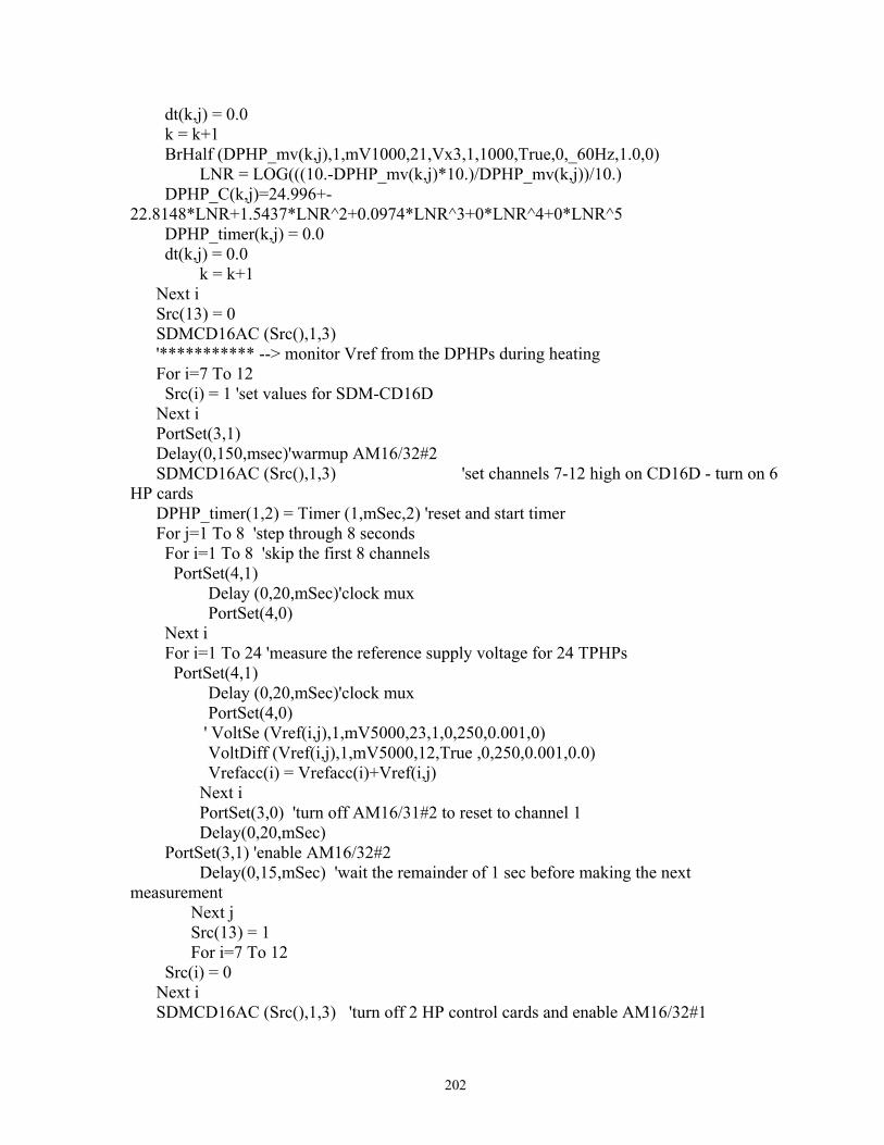
202

dt(k,j) = 0.0 k = k+1 BrHalf (DPHP_mv(k,j),1,mV1000,21,Vx3,1,1000,True,0,_60Hz,1.0,0) LNR = LOG(((10.-DPHP_mv(k,j)*10.)/DPHP_mv(k,j))/10.) DPHP_C(k,j)=24.996+-22.8148*LNR+1.5437*LNR^2+0.0974*LNR^3+0*LNR^4+0*LNR^5 DPHP_timer(k,j) = 0.0 dt(k,j) = 0.0 k = k+1 Next i Src(13) = 0 SDMCD16AC (Src(),1,3) '*********** --> monitor Vref from the DPHPs during heating For i=7 To 12 Src(i) = 1 'set values for SDM-CD16D Next i PortSet(3,1) Delay(0,150,msec)'warmup AM16/32#2 SDMCD16AC (Src(),1,3) 'set channels 7-12 high on CD16D - turn on 6 HP cards DPHP_timer(1,2) = Timer (1,mSec,2) 'reset and start timer For j=1 To 8 'step through 8 seconds For i=1 To 8 'skip the first 8 channels PortSet(4,1) Delay (0,20,mSec)'clock mux PortSet(4,0) Next i For i=1 To 24 'measure the reference supply voltage for 24 TPHPs PortSet(4,1) Delay (0,20,mSec)'clock mux PortSet(4,0) ' VoltSe (Vref(i,j),1,mV5000,23,1,0,250,0.001,0) VoltDiff (Vref(i,j),1,mV5000,12,True ,0,250,0.001,0.0) Vrefacc(i) = Vrefacc(i)+Vref(i,j) Next i PortSet(3,0) 'turn off AM16/31#2 to reset to channel 1 Delay(0,20,mSec) PortSet(3,1) 'enable AM16/32#2 Delay(0,15,mSec) 'wait the remainder of 1 sec before making the next measurement Next j Src(13) = 1 For i=7 To 12 Src(i) = 0 Next i SDMCD16AC (Src(),1,3) 'turn off 2 HP control cards and enable AM16/32#1

203

DPHP_timer_final = Timer (1,mSec,4)/1000. PortSet(3,0) '******************--> monitor DPHP temperature every 2 seconds for 80 seconds For j=2 To 41 '40 measurements every 2 seconds k = 1 For i=1 To 8 'skip first 8 channels PortSet(4,1) Delay (0,20,mSec)'clock mux PortSet(4,0) Next i For i = 1 To 8 'measure 24 probes 3 at a time, ie. 8 loops PortSet(4,1) Delay (0,20,mSec)'clock mux PortSet(4,0) BrHalf (DPHP_mv(k,j),1,mV1000,19,Vx3,1,1000,True,0,_60Hz,1.0,0) LNR = LOG(((10.-DPHP_mv(k,j)*10.)/DPHP_mv(k,j))/10.) DPHP_C(k,j)=24.996+-22.8148*LNR+1.5437*LNR^2+0.0974*LNR^3+0*LNR^4+0*LNR^5 dt(k,j) = DPHP_C(k,j) - DPHP_C(k,1) DPHP_timer(k,j) = Timer (1,mSec,4)/1000. - DPHP_timer_final k = k+1 BrHalf (DPHP_mv(k,j),1,mV1000,20,Vx3,1,1000,True,0,_60Hz,1.0,0) LNR = LOG(((10.-DPHP_mv(k,j)*10.)/DPHP_mv(k,j))/10.) DPHP_C(k,j)=24.996+-22.8148*LNR+1.5437*LNR^2+0.0974*LNR^3+0*LNR^4+0*LNR^5 dt(k,j) = DPHP_C(k,j) - DPHP_C(k,1) DPHP_timer(k,j) = Timer (1,mSec,4)/1000. - DPHP_timer_final k = k+1 BrHalf (DPHP_mv(k,j),1,mV1000,21,Vx3,1,1000,True,0,_60Hz,1.0,0) LNR = LOG(((10.-DPHP_mv(k,j)*10.)/DPHP_mv(k,j))/10.) DPHP_C(k,j)=24.996+-22.8148*LNR+1.5437*LNR^2+0.0974*LNR^3+0*LNR^4+0*LNR^5 dt(k,j) = DPHP_C(k,j) - DPHP_C(k,1) DPHP_timer(k,j) = Timer (1,mSec,4)/1000. - DPHP_timer_final k = k+1 Next i Src(13) = 0 SDMCD16AC (Src(),1,3) Delay(0,100,mSec) 'turn off mux and wait 1 sec to turn on to reset to channel 1 Src(13) = 1 SDMCD16AC (Src(),1,3) Delay(0,130,mSec) 'value was set based on the amount time it took to progress through the program Next j Src(13) = 0 SDMCD16AC (Src(),1,3)

204

'******************--> compute DPHP power and build output table For i=1 To 24 Power(i) = (Vrefacc(i)/8.0)^2 * ((DPHP_Rht(i)*DPHP_timer_final)/(DPHP_ref(i)^2*0.03)) DPHP_out(1) = DPHP_sen(i) DPHP_out(2) = DPHP_timer(i,1) DPHP_out(3) = DPHP_C(i,1) DPHP_out(4) = DPHP_mv(i,1) k = 5 For j=1 To 8 DPHP_out(k) = Vref(i,j) k = k+1 Next j DPHP_out(k) = power(i) k = k+1 DPHP_out(k) = Vrefacc(i)/8 k = k+1 DPHP_out(k) = DPHP_Rht(i) k = k+1 DPHP_out(k) = DPHP_ref(i) k = k+1 DPHP_out(k) = DPHP_timer_final k = k+1 For j=2 To 41 DPHP_out(k) = dt(i,j) k = k+1 Next j For j=2 To 41 DPHP_out(k) = DPHP_timer(i,j) k = k+1 Next j For j=2 To 41 DPHP_out(k) = DPHP_C(i,j) k = k+1 Next j For j=2 To 41 DPHP_out(k) = DPHP_mv(i,j) k = k+1 Next j CallTable DPHP Next i 'SW12 (2,0) Flag(13) = FALSE EndIf

205

'**********************--> measure all TDR theta and EC <--****************************************** If (Flag(14) = TRUE) Then 'SW12 (2,1 ) Delay (1,2,Sec) 'Measure La/L on SDMX50 mux TDR100 (TDRraw(),4,0,1002,4,1.0,251,15,3,0.3,0.155,1.0,0) For i=1 To 2 LaL(i) = TDRraw(i) Next i TDR100 (TDRraw(),4,0,6108,4,1.0,251,17.2,3,0.3,0.155,1.0,0) For i=1 To 8 LaL(i+2) = TDRraw(i) Next i TDR100 (TDRraw(),4,0,7108,4,1.0,251,18.4,3,0.3,0.155,1.0,0) For i=1 To 8 LaL(i+10) = TDRraw(i) Next i TDR100 (TDRraw(),4,0,8108,4,1.0,251,18.4,3,0.3,0.155,1.0,0) For i=1 To 8 LaL(i+18) = TDRraw(i) Next i ' measure EC TDR100 (TDRraw(),4,3,1002,4,1.0,251,15,5,0.3,0.155,1.0,0.0) For i=1 To 2 TDR_EC(i) = TDRraw(i) Next i TDR100 (TDRraw(),4,3,6108,4,1.0,251,17.2,5,0.3,0.155,1.0,0.0) For i=1 To 8 TDR_EC(i+2) = TDRraw(i) Next i TDR100 (TDRraw(),4,3,7108,4,1.0,251,18.4,5,0.3,0.155,1.0,0.0) For i=1 To 8 TDR_EC(i+10) = TDRraw(i) Next i TDR100 (TDRraw(),4,3,8108,4,1.0,251,18.4,5,0.3,0.155,1.0,0.0) For i=1 To 8 TDR_EC(i+18) = TDRraw(i) Next i ' compute K and build output table For i=1 To 26 LaL2(i) = LaL(i)^2 'apparent dielectric constant K = (La/L)^2 ToppVWC(i) = a0 + a1*LaL2(i) + a2*LaL2(i)^2 + a3*LaL2(i)^3

206

TDR_out(1) = TDR_sen(i) TDR_out(2) = LaL(i) TDR_out(3) = ToppVWC(i) TDR_out(4) = TDR_EC(i) TDR_out(5) = a0 TDR_out(6) = a1 TDR_out(7) = a2 TDR_out(8) = a3 CallTable TDR Next i 'SW12 (2,0) Flag(14)=False EndIf '**********************--> measure all TDR waveforms only <--****************************************** If (Flag(15) = TRUE) Then 'SW12 (2,1 ) Delay (1,2,Sec) 'SDMX50 (5,1) 'Measure Waveform on SDMX50 mux TDR100 (WavePT(),4,1,1001,4,1.0,251,15.0,3,0.3,0.155,1000.,0) MuxChan=TDR_sen(1) CallTable TDR_Wave() ' TDR100 (WavePT(),4,1,2001,4,1.0,251,15.0,3,0.3,0.155,1000.,0) MuxChan=TDR_sen(2) CallTable TDR_Wave() ' TDR100 (WavePT(),4,1,6101,4,1.0,251,17.2,3,0.3,0.155,1000.,0) MuxChan=TDR_sen(3) CallTable TDR_Wave() ' TDR100 (WavePT(),4,1,6201,4,1.0,251,17.2,3,0.3,0.155,1000.,0) MuxChan=TDR_sen(4) CallTable TDR_Wave() ' TDR100 (WavePT(),4,1,6301,4,1.0,251,17.2,3,0.3,0.155,1000.,0) MuxChan=TDR_sen(5) CallTable TDR_Wave() ' TDR100 (WavePT(),4,1,6401,4,1.0,251,17.2,3,0.3,0.155,1000.,0) MuxChan=TDR_sen(6) CallTable TDR_Wave()

207

' TDR100 (WavePT(),4,1,6501,4,1.0,251,17.2,3,0.3,0.155,1000.,0) MuxChan=TDR_sen(7) CallTable TDR_Wave() ' TDR100 (WavePT(),4,1,6601,4,1.0,251,17.2,3,0.3,0.155,1000.,0) MuxChan=TDR_sen(8) CallTable TDR_Wave() ' TDR100 (WavePT(),4,1,6701,4,1.0,251,17.2,3,0.3,0.155,1000.,0) MuxChan=TDR_sen(9) CallTable TDR_Wave() ' TDR100 (WavePT(),4,1,6801,4,1.0,251,17.2,3,0.3,0.155,1000.,0) MuxChan=TDR_sen(10) CallTable TDR_Wave() ' TDR100 (WavePT(),4,1,7101,4,1.0,251,18.4,3,0.3,0.155,1000.,0) MuxChan=TDR_sen(11) CallTable TDR_Wave() ' TDR100 (WavePT(),4,1,7201,4,1.0,251,18.4,3,0.3,0.155,1000.,0) MuxChan=TDR_sen(12) CallTable TDR_Wave() ' TDR100 (WavePT(),4,1,7301,4,1.0,251,18.4,3,0.3,0.155,1000.,0) MuxChan=TDR_sen(13) CallTable TDR_Wave() ' TDR100 (WavePT(),4,1,7401,4,1.0,251,18.4,3,0.3,0.155,1000.,0) MuxChan=TDR_sen(14) CallTable TDR_Wave() ' TDR100 (WavePT(),4,1,7501,4,1.0,251,18.4,3,0.3,0.155,1000.,0) MuxChan=TDR_sen(15) CallTable TDR_Wave() ' TDR100 (WavePT(),4,1,7601,4,1.0,251,18.4,3,0.3,0.155,1000.,0) MuxChan=TDR_sen(16) CallTable TDR_Wave() ' TDR100 (WavePT(),4,1,7701,4,1.0,251,18.4,3,0.3,0.155,1000.,0) MuxChan=TDR_sen(17) CallTable TDR_Wave() ' TDR100 (WavePT(),4,1,7801,4,1.0,251,18.4,3,0.3,0.155,1000.,0)

208

MuxChan=TDR_sen(18) CallTable TDR_Wave() ' TDR100 (WavePT(),4,1,8101,4,1.0,251,18.4,3,0.3,0.155,1000.,0) MuxChan=TDR_sen(19) CallTable TDR_Wave() ' TDR100 (WavePT(),4,1,8201,4,1.0,251,18.4,3,0.3,0.155,1000.,0) MuxChan=TDR_sen(20) CallTable TDR_Wave() ' TDR100 (WavePT(),4,1,8301,4,1.0,251,18.4,3,0.3,0.155,1000.,0) MuxChan=TDR_sen(21) CallTable TDR_Wave() ' TDR100 (WavePT(),4,1,8401,4,1.0,251,18.4,3,0.3,0.155,1000.,0) MuxChan=TDR_sen(22) CallTable TDR_Wave() ' TDR100 (WavePT(),4,1,8501,4,1.0,251,18.4,3,0.3,0.155,1000.,0) MuxChan=TDR_sen(23) CallTable TDR_Wave() ' TDR100 (WavePT(),4,1,8601,4,1.0,251,18.4,3,0.3,0.155,1000.,0) MuxChan=TDR_sen(24) CallTable TDR_Wave() ' TDR100 (WavePT(),4,1,8701,4,1.0,251,18.4,3,0.3,0.155,1000.,0) MuxChan=TDR_sen(25) CallTable TDR_Wave() ' TDR100 (WavePT(),4,1,8801,4,1.0,251,18.4,3,0.3,0.155,1000.,0) MuxChan=TDR_sen(26) CallTable TDR_Wave() ' 'SW12 (2,0) Flag(15)=False EndIf '**********************************--> measure ECHO <--************************************************* 'code modified from: Colin Campbell; date: February 23, 2006 If (Flag(16) = True) Then

209

SW12 (2,1) Delay (0,30,mSec) SerialFlush (Com1) SerialFlush (Com4) Delay (0,1,Sec) SerialIn (TEout(1),Com1,200,0,1000) SerialIn (TEout(2),Com4,200,0,1000) For i = 1 To TE_Num If TEout(i) <> "" Then Pos_RawVWC(i) = InStr (1,TEout(i),"String",0) Pos_RawEC(i) = InStr(Pos_RawVWC(i) ,TEout(i),CHR(32),2)+1 Pos_RawT(i) = InStr(Pos_RawEC(i),TEout(i),CHR(32),2)+1 RawVWC(i)=Mid (TEout(i),Pos_RawVWC(i),Pos_RawEC(i)-Pos_RawVWC(i)) RawEC(i)=Mid (TEout(i),Pos_RawEC(i),Pos_RawT(i)-Pos_RawEC(i)) RawT(i)=Mid (TEout(i),Pos_RawT(i),3) Temp(i)= (RawT(i)-400)/10 VWCm(i)= RawVWC(i)*.00109 - .629 ' Use for mineral soil VWCp(i)= 0.00104*RawVWC(i)-.499 ' Use for potting soil ECb(i) = RawEC(i)/100 eb(i) = 7.64E-8*RawVWC(i)^3 - 8.85E-5*RawVWC(i)^2 +4.85E-02*RawVWC(i)-10 ep(i) = 80.3 - 0.37*(Temp(i)- 20) If VWCm(i) > 0.10 Then ECp(i) = (ep(i)*ECb(i))/(eb(i)-eb0) Else ECp(i) = ECb(i) EndIf Else TEout(i) = "No Probe" EndIf Next i SW12 (2,0) CallTable (TEData) Flag(16) = False EndIf NextScan SlowSequence Scan (1,Min,3,0) AM25T (Scale_temp_C,1,mV20C,25,9,TypeT,TRef,4 ,6,Vx2,True ,500,250,1.0,0) NextScan EndProg

210


211

APPENDIX I. LOGGERNET PROGRAM FOR LYSIMETER 2

'CR3000 Series Datalogger ' SEPHAS Lysimeter 2 ' program by Brad F Lyles ' current version 2.4 (my) ' ' May 27, 2008 '... Modified from Tank3_v1_1.cr3 ' Changed TPMP and DPHP sensor numbers and Rref anf Rheater ' ' Modified 5-29-08 added Ref and heater resitance for TPHP and DPHP sensors, ' changed sensor code for upper four TPHP sensors from 210203 to 220203. ' ' V1_3 modified 6-12-08 by Brad Lyles: ' fixed TDR cable length offset ' added code to turn on heater card DC power contactor ' ' ver 2_2 6-17-08 Brad Lyles ' modified from Tank1 v2.2 ' modified with new output format for TPHP, DPHP, HDU, scale and TDR ' modified code for CO2 sensors - changed from ppm to percent to match sensors, set to measure every 15 minutes ' changed output format for table "scale" to include sensorID and calibration coeficients for SHF ' changed TPHP and DPHP format to use initial temperature before heated started rather than the first measurement ' after heated stopped. ' changed TPHP and DPHP output format to list differential temperature as a block that can be easilly plotted. ' changed the time into from 55 to 0 to that the table time stamps would be on the hour ' added if then statement to save old shf calib if newly computed value was zero ' moved TDR to be measured at moderate frquency ' added code to measure upper 10 TDRs hourly ' ' ver 2_3 6-17-08 Brad Lyles ' fixed programming error in the DPHP_out stream ' added 1 sec delay after turning on SDM via sw12_2 ' ' ver 2_4 07-15-08 Skipped - MY ' ' ver 2_5 07-15-08 Michael Young ' -- MY - IF/THEN statements were added to shut down high resolution measurements at the time that low ' resolution measurements are being taken. These changes to the code are marked by "MOD by MY" in

212

' commented line preceding change. MY increased cable lengths for the TDR probes to increase upper ' end of water content measurement capability. New cable lengths are as shown. Probe offset also change ' from 0.085 to 0.115, based on laboratory measurements made by Karletta Chief. ' --B Lyles changed table allocation values to allow 10 days storage on logger ' ' ver 2_6 7-25-08 Skipped BFL ' ' Ver Tank3_2_7 7-25-08 Brad Lyles ' applied same changes as were applied to tank 1 ver 2_7, as follows: ' moved ECHO sensors into a slow sequence every 5 minutes ' remove SW12 (2,1) commands from all but the ECHO probe in the if FLAG 16 command sequence ' changed soil heat flux time into interval from "Min" to "3" ' alter method for obtaining data from scale - 100 measurements in single burst ' modified code to write data to cards if present (assumed 4mb in logger and 2Gb on card to determine size). ' removed HF_scale table ' changed scan interval from 1 Sec to 250 mSec ' ' Ver 2_8 8-8-08 Brad Lyles ' changed soil heat flux code to match tank 1 and Eddy code ' changed DPHP Vref mesurement from single eneded to differential ' ' Ver 2_9 8-15-08 Brad Lyles ' changed TPHP Vref measurement from single ended to differential ' changed TPHP Rref values (1-4) set the remainder to 1.0 ' ' Ver 2_10 8-19-08 Brad Lyles ' changed SHF to measure at 16 after the hour until 19 after rather than 1 and 3 minutes after ' (SHF calib was not initiating properly due to a table over run at the top of the hour) ' changed ECHO code - move code from slow sequence back to the main routine, and changed ' maeasurement delay from 100 to 200 dSec ' wired CO2 sensors to mux ' updated Rref values for TPHP (5-18) ' ' Ver 2_11 10-10-08 Brad Lyles ' added a line of code to measure the time during the TPHP cooling cycle ' changed the delay in the TPHP heating from 370 to 365 mS so we would no longer get 8 seconds exactly ' ' Ver 2_12 10-23-08 Brad Lyles ' changed code to include TDR calibration factors

213

' changed code to compute HDU T* and matrix potential values and included calibration factors ' added code to measure scale temp on AM25T#2 chan 25 in slow sequence ' ' Ver 2_13 12-3-08 Brad Lyles ' added code to compute intermediate statistics for scale in scratch table ' removed code to manually compute scale statistics ' added debug table to intermediate statics table ' added code to test HDU_Tstar, if < 0 then = 1e-6 ' added code to convert CO2 fractional percent to ppm ' ' Ver 2_14 12-16-08 Brad Lyles ' changed ECHO VWC from p (potting soil) to m (mineral soil) in ECHO table. ' fixed HDU section programing errors: sensors 17-32 were not assigned to proper calibration wet and dry ' calibration coeficients; therefore, all Tstar and calib coefs are in error prior to this date. ' cleaned up TDR_sen(13-15) redundency - this error should not have caused any errors ' changed the HDU hourly sensors from 8 to 16; turned on CE8#2 and measured more sensors ' ' Ver 2_17 2-5-09 Brad Lyles (note: skipped ver2_15 and Ver2_16 to match tank3) ' changed sensor IDs for the top four TPHPs ' changed TEdata table output to include sensor IDs ' 'Wiring 'H1 = scale (red) 'L1 = scale (white) 'G = scale (black) 'H2 = S_Therm(1) (red) 'L2 = S_Therm(2) (red) 'G = purple, clear (1&2) 'H3 = S_Therm(3) (red) 'L3 = S_Therm(4) (red) 'G = purple, clear (3&4) 'H4 = TCAV(1) 'L4 = TCAV(1) 'G = 'H5 = SHF V_Rf(1) yellow 'L5 = SHF V_Rf(2) yellow 'G = purple, clear 'H6 = SHF(1) white 'L6 = SHF(1) green 'G = clear 'H7 = SHF(2) white 'L7 = SHF(2) green 'G = clear

214

'H8 = HDU AM25T#1 Hi 'L8 = HDU AM25T#1 Lo 'G = 'H9 = HDU AM25T#2 Hi 'L9 = HDU AM25T#2 Lo 'G = 'H10 = DPHP & TPHP AM16/32#1 even Lo 'L10 = DPHP & TPHP AM16/32#1 odd Hi 'G = 'H11 = DPHP & TPHP AM16/32#1 odd Lo 'L11 = CS616 (green) 'G = 'H12 = Vref AM16/32#2 even Lo 'L12 = 'G = 'H13 = VDIV10.1 to AM16/32 #3 even Hi CO2 sensors 'L13 = VDIV10.1 to AM16/32 #3 even Lo CO2 sensors 'G = 'H14 = 'L14 = 'G = 'VX1 = scale (green) 'VX2 = AM25T 'G = scale (yellow) 'VX3 = DPHP AM16/32#1 even Hi 'VX4 = 108 probes 1-4 (black) 'G = 'SW12_1 = SHF auto calibration (red) 'SW12_2 = TDR100 and ECHO (1&2) 'G = SHF (black) 'C1 = Tx 'C2 = Rx ECHO #3 'C3 = enable AM16/32 #2 'C4 = clock all mux 'C5 = enable AM25T #1 'C6 = enable AM25T #2 'C7 = Tx 'C8 = Rx ECHO #4 'G = 'SDM_C1 = SDMCD16D & TDR100 & tdr mux 'SDM_C2 = SDMCD16D & TDR100 & tdr mux 'SDM_C3 = SDMCD16D & TDR100 & tdr mux 'G = '5V = CS-616 (orange) ' ' ECHO TE

215

'SW12V-2 ALL WHITE (EXCITATION) WIRES 'C2 TE #1 OUTPUT (RED) WIRE 'C8 TE #2 OUTPUT (RED) WIRE 'GND ALL BARE (GND) WIRES 'Flags 'Flag(1) = High Freqency Sample Mode 'Flag(2) = Moderate Sample Freq. Sensor Set 'Flag(3) = Intermediate Sample Freq. Sensor Set 'Flag(4) = Low Sample Freq. Sensor Set 'Flag(10) = all CO2 sensors 'Flag(11) = all HDU sensors 'Flag(12) = all TPHP sensors 'Flag(13) = all DPHP sensors 'Flag(14) = all TDR sensors 'Flag(15) = all TDR waveforms 'Flag(16) = ECHO TE sensors 'SDM CD16D channels defs 'chan(1) = CE8(1) 'chan(2) = CE8(2) 'chan(3) = CE8(3) 'chan(4) = CE8(4) 'chan(5) = TPHP heater card (1-4) 'chan(6) = DPHP heater card (5-7) 'chan(7) = 'chan(8) = 'chan(9) = 'chan(10) = 'chan(11) = 'chan(12) = enable AM16/32 #4 (output from CO2 sensors) 'chan(13) = enable AM16/32 #1 (output from TPHP sensors) 'chan(14) = enable AM16/32 #3 (output from DPHP sensors)(2 TPHPs here also) 'chan(15) = control contactor for heater boards via A21REL-12 'chan(16) = SequentialMode 'Output period Const OUTPUT_INTERVAL = 15 'data output interval in minutes. Const CAL_INTERVAL = 1440 'HFP01SC insitu calibration interval (minutes). Const END_CAL = OUTPUT_INTERVAL-1 'End HFP01SC insitu calibration one minute before the next Output.

216

Const HFP01SC_CAL_1 = 1000/61.5 'Unique multiplier for HFP01SC #1 (1000/sensitivity). Const HFP01SC_CAL_2 = 1000/61.0 'Unique multiplier for HFP01SC #2 (1000/sensitivity). 'Declare Public Variables Public Scale_mV, Scale_Kg, ScaleMult, ScaleTar, Scale_array(5) Public Scale_Kg_SD, Scale_Kg_Min, Scale_Kg_Max, Scale_Kg_Mean, Scale_mV_Mean Public batt_volt, Scale_temp_C Public Ptemp Public Flag(16) As Boolean Public Src(16) Dim HDU_output_flag As Boolean Public Scale_flag As Boolean Public old_ScaleKg, del_Scale, HF_event Dim MassID Dim ST_ID Dim TCAV_ID Dim SHF1_ID Dim SHF2_ID Dim ST1_ID, ST2_ID, ST3_ID, ST4_ID Dim Ptemp_ID Dim CS616_ID Public shf(2) Public tcav_1 Public cs616_uS 'Water content reflectometer period. Public cs616_uS_tc Public soil_water_VMC 'Volumetric soil water content with temperature correction. Public S_Therm(4) Public shf_cal(2) Units shf = W/m^2 Units cs616_uS = uSeconds Units soil_water_VMC = frac_v_wtr Units shf_cal = W/(m^2 mV) Units S_therm() = C Dim sw12_1_state 'State of the switched 12Vdc port 1. 'Soil heat flux calibration variables. Dim shf_mV(2) Dim shf_mV_run(2) Dim shf_mV_0(2) Dim shf_mV_180(2) Dim shf_mV_end(2)

217

Dim V_Rf(2) Dim V_Rf_run(2) Dim V_Rf_180(2) Dim shf_cal_on As Boolean Dim shf_calib Public TRef Public ST1(16), ST2(16), Public del_T1(16), del_T2(16) Public T1_1sec(16), T2_1sec(16) Public T1_30sec(16), T2_30sec(16) Dim HDU_sen(32) Dim HDU_wet(32) Dim HDU_dry(32) Dim HDU_alpha(32) Dim HDU_beta(32) Dim HDU_Tstar Dim HDU_Psi Public HDU_out(12) Units Scale_mV = mV Units Scale_Kg = Kg Units ST1 = deg C Units ST1 = deg C Units del_T1 = deg C Units del_T2 = deg C Units T1_1sec = deg C Units T2_1sec = deg C Units T1_30sec = deg C Units T2_30sec = deg C Public Vref(18,8),Vrefacc(18), Power(18), LNR Public DPHP_mv(15,41), DPHP_C(15,41), DPHP_out(200) Public DPHP_timer(15,41), DPHP_timer_final Public DPHP_ref(14), DPHP_Rht(14), DPHP_sen(14), dt(15,41) Public TPHP_mV1(18,41), TPHP_C1(18,41), TPHP_sen(18) Public TPHP_mV2(18,41), TPHP_C2(18,41),dT1(18,41), dT2(18,41) Public TPHP_ref(18), TPHP_Rht(18) Public TPHP_out(302) Public TPHP_timer(18,49), TPHP_timer_final Public LaL(26), LaL2(26) Public TDR_EC(26), ToppVWC(26) Public WavePT(260), MuxChan, TDR_sen(26)

218

Public TDR_out(8), TDRraw(8) Const a0 = -0.053 Const a1 = 0.0292 Const a2 = -0.00055 Const a3 = 0.0000043 Const high = true Const low = false 'Declare Other Variables Dim i,j, k, kk Dim ProbeNum 'Declare ECHO Public Variables Const TE_Num = 2 'change this constant for the number of ECHO TE probes you are reading '4 is the maximum number of TE probes readable without a multiplexer Const eb0 = 6 'empirical constant loosely representing the dielectric of dry soil Public TEout(TE_Num,1) As String * 32 Public Pos_RawVWC(TE_Num) as LONG Public Pos_RawEC(TE_Num) as LONG Public Pos_RawT(TE_Num) as LONG Public RawVWC(TE_Num) as LONG,RawEC(TE_Num) as FLOAT,RawT(TE_Num) as LONG Public VWCm(TE_Num) As Float,VWCp(TE_Num) As Float 'VWCm for mineral soil, VWCp for potting soil public Temp(TE_Num) as FLOAT Public eb(TE_Num) as float, ep(TE_Num) as float 'eb is bulk dielectric and ep is the 'dielectric of the pore water Public ECb(TE_Num) as float ' this is bulk dielectric measured by the TE Public ECp(TE_Num) as float ' this is the pore water dielectric estimated by Public x As Float Public TE_sen(TE_Num) 'Declare Viasala CO2 Sensor Public Variables Public CO2_volt Public CO2_pct, CO2_ppm Public CO2_sensor(4), sensor_num 'Define Data Tables

219

DataTable (TEData,True,96) CardOut (0 ,48000) Sample (TE_Num,TE_sen(),IEEE4) Sample (TE_Num, VWCm(),FP2) Sample (TE_Num,ECp(),FP2) Sample (TE_Num,Temp(),FP2) EndTable 'Define Data Tables DataTable (Daily,1,40) CardOut (0 ,20000) DataInterval (0,1440,Min,10) Average (1,Scale_Kg,FP2,False) StdDev (1,Scale_Kg,FP2,False) Minimum (1,Scale_Kg,FP2,False,False) Maximum (1,Scale_Kg,FP2,False,False) Minimum (1,batt_volt,FP2,0,False) Sample (1,Ptemp,FP2) EndTable DataTable (TDR_Wave,True,104) CardOut (0 ,52000) Sample(1,MuxChan,IEEE4) Sample(260,WavePT(),FP2) FieldNames ("sensorID:,WavePT_1:,WavePT_2:,WavePT_3:,etc") EndTable DataTable (TDR,True,1376) CardOut (0 ,688000) Sample(8,TDR_out(),IEEE4) FieldNames ("sensorID:,LaL:,ToppVWC:,TDR_EC") EndTable DataTable (Scale,True,-1) CardOut (0 ,-1) DataInterval (0,OUTPUT_INTERVAL,Min,0) Sample (1,MassID,IEEE4) Average (1,Scale_mV,IEEE4,False) Sample (1,Scale_Kg_Mean,IEEE4) Sample (1,Scale_Kg_SD,IEEE4) Sample (1,Scale_Kg_Min,IEEE4) Sample (1,Scale_Kg_Max,IEEE4) Sample (1,TCAV_ID,IEEE4) Average (1,tcav_1,FP2,False)

220

Sample (1,SHF1_ID,IEEE4) Average (1,shf(1),IEEE4,shf_cal_on) Sample (1,shf_cal(1),IEEE4) Sample (1,SHF2_ID,IEEE4) Average (1,shf(2),IEEE4,shf_cal_on) Sample (1,shf_cal(2),IEEE4) Sample (1,ST1_ID,IEEE4) Average (1,S_Therm(1),FP2,False) Sample (1,ST2_ID,IEEE4) Average (1,S_Therm(2),FP2,False) Sample (1,ST3_ID,IEEE4) Average (1,S_Therm(3),FP2,False) Sample (1,ST4_ID,IEEE4) Average (1,S_Therm(4),FP2,False) Sample (1,ptemp_ID,IEEE4) Average (1,Ptemp,FP2,False) Average (1,Scale_temp_C,FP2,False) EndTable DataTable (HDU,true,896) CardOut (0 ,448000) Sample(12,HDU_out(),IEEE4) FieldNames ("sensorID:,SoilTemp:,deltaTemp:,T_1sec:,T_30sec:,RefTemp:,Tstar:,Psi:,wet:,dry:,alpha:,beta") EndTable DataTable (DPHP,Flag(13),1344) CardOut (0 ,672000) Sample (179,DPHP_out(),IEEE4) FieldNames ("sensorID:,timer_1:,temp_C_1:,temp_mV_1:,Vref1:,Vref2:,Vref3:,Vref4:,Vref5:,Vref6:,Vref7:,Vref8:,Power:,Vref:avg,Rht:,Rref:,heat_time:total") EndTable DataTable (TPHP,Flag(12),1728) CardOut (0 ,864000) Sample (302,TPHP_out(),IEEE4) FieldNames ("sensorID:,timer_1:,temp1_C_1:,temp1_mV_1:,temp2_C_1:,temp2_mv_1:,Vref1:,Vref2:,Vref3:,Vref4:,Vref5:,Vref6:,Vref7:,Vref8:,Power:,Vref:avg,Rht:,Rref:,heat_time:total") EndTable DataTable (CO2,Flag(10),1536) CardOut (0 ,768000) Sample (1,sensor_num,IEEE4)

221

Sample (1,CO2_ppm,IEEE4) Sample (1,CO2_volt,IEEE4) EndTable DataTable (scale_int,true,20) DataInterval (57,60,Sec,10) Average (1,Scale_mV,IEEE4,False) Average (1,Scale_Kg,IEEE4,False) StdDev (1,Scale_Kg,IEEE4,False) Minimum (1,Scale_Kg,IEEE4,False,False) Maximum (1,Scale_Kg,IEEE4,False,False) EndTable 'Subroutines Sub Initialize MassID = 200015 TCAV_ID = 220208 SHF1_ID = 210207 SHF2_ID = 230207 ST1_ID = 260206 ST2_ID = 260406 ST3_ID = 260506 ST4_ID = 260706 Ptemp_ID = 200016 'reset SDM-CD16D For i=1 To 16 Src(i) = 0.0 Next i ' HDU HDU_sen(1) = 210204 HDU_sen(2) = 220204 HDU_sen(3) = 230204 HDU_sen(4) = 240204 HDU_sen(5) = 210304 HDU_sen(6) = 220304 HDU_sen(7) = 230304 HDU_sen(8) = 240304 HDU_sen(9) = 210404 HDU_sen(10) = 220404 HDU_sen(11) = 230404 HDU_sen(12) = 240404 HDU_sen(13) = 210504 HDU_sen(14) = 220504 HDU_sen(15) = 230504 HDU_sen(16) = 240504

222

HDU_sen(17) = 210704 HDU_sen(18) = 220704 HDU_sen(19) = 230704 HDU_sen(20) = 240704 HDU_sen(21) = 210904 HDU_sen(22) = 220904 HDU_sen(23) = 230904 HDU_sen(24) = 240904 HDU_sen(25) = 211104 HDU_sen(26) = 221104 HDU_sen(27) = 231104 HDU_sen(28) = 241104 HDU_sen(29) = 221304 HDU_sen(30) = 241304 HDU_sen(31) = 211404 HDU_sen(32) = 231404 HDU_dry(1) = 2.78951132 HDU_dry(2) = 2.869471 HDU_dry(3) = 2.83114116 HDU_dry(4) = 2.65123728 HDU_dry(5) = 2.7289936 HDU_dry(6) = 2.73284736 HDU_dry(7) = 2.8554494 HDU_dry(8) = 2.59175868 HDU_dry(9) = 2.669614 HDU_dry(10) = 2.7065804 HDU_dry(11) = 2.75070072 HDU_dry(12) = 2.60116448 HDU_dry(13) = 2.85971376 HDU_dry(14) = 2.95064272 HDU_dry(15) = 2.8460672 HDU_dry(16) = 2.73349148 HDU_dry(17) = 2.80577644 HDU_dry(18) = 2.77156408 HDU_dry(19) = 2.72642328 HDU_dry(20) = 2.63493796 HDU_dry(21) = 2.88133936 HDU_dry(22) = 2.7820248 HDU_dry(23) = 2.84700376 HDU_dry(24) = 2.85843296 HDU_dry(25) = 2.77279664 HDU_dry(26) = 2.98083128 HDU_dry(27) = 2.96812904 HDU_dry(28) = 2.91877672 HDU_dry(29) = 2.81746116 HDU_dry(30) = 2.92262956

223

HDU_dry(31) = 2.74507848 HDU_dry(32) = 2.81222672 HDU_wet(1) = 0.7366201 HDU_wet(2) = 0.758392769 HDU_wet(3) = 0.764136838 HDU_wet(4) = 0.742934162 HDU_wet(5) = 0.44876152 HDU_wet(6) = 0.642346788 HDU_wet(7) = 0.778601715 HDU_wet(8) = 0.722264946 HDU_wet(9) = 0.668654096 HDU_wet(10) = 0.644992908 HDU_wet(11) = 0.655471876 HDU_wet(12) = 0.642211308 HDU_wet(13) = 0.660179668 HDU_wet(14) = 0.655511928 HDU_wet(15) = 0.652714928 HDU_wet(16) = 0.6694899 HDU_wet(17) = 0.725214544 HDU_wet(18) = 0.657790148 HDU_wet(19) = 0.641952056 HDU_wet(20) = 0.626047516 HDU_wet(21) = 0.761619496 HDU_wet(22) = 0.683809436 HDU_wet(23) = 0.724266516 HDU_wet(24) = 0.760557324 HDU_wet(25) = 0.726621312 HDU_wet(26) = 0.808561404 HDU_wet(27) = 0.749494704 HDU_wet(28) = 0.77700866 HDU_wet(29) = 0.762851712 HDU_wet(30) = 0.784387052 HDU_wet(31) = 0.751563488 HDU_wet(32) = 0.737108228 HDU_alpha(1) = 130.6060899 HDU_alpha(2) = 130.6060899 HDU_alpha(3) = 130.6060899 HDU_alpha(4) = 130.6060899 HDU_alpha(5) = 157.1680554 HDU_alpha(6) = 157.1680554 HDU_alpha(7) = 130.6060899 HDU_alpha(8) = 130.6060899 HDU_alpha(9) = 114.243419 HDU_alpha(10) = 114.243419 HDU_alpha(11) = 114.243419

224

HDU_alpha(12) = 114.243419 HDU_alpha(13) = 114.243419 HDU_alpha(14) = 114.243419 HDU_alpha(15) = 114.243419 HDU_alpha(16) = 114.243419 HDU_alpha(17) = 114.243419 HDU_alpha(18) = 114.243419 HDU_alpha(19) = 114.243419 HDU_alpha(20) = 114.243419 HDU_alpha(21) = 114.243419 HDU_alpha(22) = 114.243419 HDU_alpha(23) = 114.243419 HDU_alpha(24) = 114.243419 HDU_alpha(25) = 114.243419 HDU_alpha(26) = 114.243419 HDU_alpha(27) = 114.243419 HDU_alpha(28) = 114.243419 HDU_alpha(29) = 114.243419 HDU_alpha(30) = 114.243419 HDU_alpha(31) = 114.243419 HDU_alpha(32) = 114.243419 HDU_beta(1) = 0.249905573 HDU_beta(2) = 0.262758755 HDU_beta(3) = 0.260799556 HDU_beta(4) = 0.243596244 HDU_beta(5) = 0.272491631 HDU_beta(6) = 0.311440296 HDU_beta(7) = 0.251064942 HDU_beta(8) = 0.246999356 HDU_beta(9) = 0.259158783 HDU_beta(10) = 0.25370323 HDU_beta(11) = 0.260864937 HDU_beta(12) = 0.236992011 HDU_beta(13) = 0.342610495 HDU_beta(14) = 0.327322061 HDU_beta(15) = 0.30303095 HDU_beta(16) = 0.277840458 HDU_beta(17) = 0.346524893 HDU_beta(18) = 0.344764577 HDU_beta(19) = 0.319645425 HDU_beta(20) = 0.318748375 HDU_beta(21) = 0.258992949 HDU_beta(22) = 0.289460977 HDU_beta(23) = 0.308682937 HDU_beta(24) = 0.330449133 HDU_beta(25) = 0.259906384

225

HDU_beta(26) = 0.268066579 HDU_beta(27) = 0.259740055 HDU_beta(28) = 0.29257136 HDU_beta(29) = 0.244463622 HDU_beta(30) = 0.273629745 HDU_beta(31) = 0.266353255 HDU_beta(32) = 0.298036951 ' TPHP TPHP_ref(1) = 1.002 TPHP_ref(2) = 1.002 TPHP_ref(3) = 1.0005 TPHP_ref(4) = 1.0027 TPHP_ref(5) = 0.99841 TPHP_ref(6) = 0.99967 TPHP_ref(7) = 1.0007 TPHP_ref(8) = 0.99836 TPHP_ref(9) = 0.99869 TPHP_ref(10) = 0.99902 TPHP_ref(11) = 1.0018 TPHP_ref(12) = 0.99827 TPHP_ref(13) = 0.99925 TPHP_ref(14) = 0.99617 TPHP_ref(15) = 1.0024 TPHP_ref(16) = 1.0008 TPHP_ref(17) = 0.99841 TPHP_ref(18) = 0.99892 TPHP_Rht(1) = 40.1 TPHP_Rht(2) = 40.3 TPHP_Rht(3) = 39.6 TPHP_Rht(4) = 40.0 TPHP_Rht(5) = 40.3 TPHP_Rht(6) = 40.6 TPHP_Rht(7) = 40.7 TPHP_Rht(8) = 39.9 TPHP_Rht(9) = 39.7 TPHP_Rht(10) = 40.1 TPHP_Rht(11) = 40.4 TPHP_Rht(12) = 39.5 TPHP_Rht(13) = 40.0 TPHP_Rht(14) = 40.0 TPHP_Rht(15) = 40.1 TPHP_Rht(16) = 39.6 TPHP_Rht(17) = 40.5 TPHP_Rht(18) = 39.8 TPHP_sen(1) = 225003

226

TPHP_sen(2) = 225103 TPHP_sen(3) = 225203 TPHP_sen(4) = 225303 TPHP_sen(5) = 210303 TPHP_sen(6) = 220303 TPHP_sen(7) = 230303 TPHP_sen(8) = 240303 TPHP_sen(9) = 210403 TPHP_sen(10) = 220403 TPHP_sen(11) = 230403 TPHP_sen(12) = 240403 TPHP_sen(13) = 210503 TPHP_sen(14) = 220503 TPHP_sen(15) = 230503 TPHP_sen(16) = 240503 TPHP_sen(17) = 220703 TPHP_sen(18) = 240703 'DPHP DPHP_ref(1) = 1.016 DPHP_ref(2) = 1.017 DPHP_ref(3) = 1.019 DPHP_ref(4) = 1.017 DPHP_ref(5) = 1.016 DPHP_ref(6) = 1.020 DPHP_ref(7) = 1.013 DPHP_ref(8) = 1.022 DPHP_ref(9) = 1.023 DPHP_ref(10) = 1.015 DPHP_ref(11) = 1.014 DPHP_ref(12) = 1.021 DPHP_ref(13) = 1.016 DPHP_ref(14) = 1.016 DPHP_Rht(1) = 39.6 DPHP_Rht(2) = 40.0 DPHP_Rht(3) = 39.5 DPHP_Rht(4) = 39.7 DPHP_Rht(5) = 39.5 DPHP_Rht(6) = 39.4 DPHP_Rht(7) = 40.0 DPHP_Rht(8) = 39.5 DPHP_Rht(9) = 39.6 DPHP_Rht(10) = 39.7 DPHP_Rht(11) = 39.7 DPHP_Rht(12) = 40.0 DPHP_Rht(13) = 39.9 DPHP_Rht(14) = 39.8

227

DPHP_sen(1) = 210702 DPHP_sen(2) = 230702 DPHP_sen(3) = 210902 DPHP_sen(4) = 220902 DPHP_sen(5) = 230902 DPHP_sen(6) = 240902 DPHP_sen(7) = 211102 DPHP_sen(8) = 221102 DPHP_sen(9) = 231102 DPHP_sen(10) = 241102 DPHP_sen(11) = 221302 DPHP_sen(12) = 241302 DPHP_sen(13) = 211402 DPHP_sen(14) = 231402 'TDR TDR_sen(1) = 210301 TDR_sen(2) = 220301 TDR_sen(3) = 230301 TDR_sen(4) = 240301 TDR_sen(5) = 210401 TDR_sen(6) = 220401 TDR_sen(7) = 230401 TDR_sen(8) = 240401 TDR_sen(9) = 210501 TDR_sen(10) = 220501 TDR_sen(11) = 230501 TDR_sen(12) = 240501 TDR_sen(13) = 210701 TDR_sen(14) = 220701 TDR_sen(15) = 230701 TDR_sen(16) = 240701 TDR_sen(17) = 210901 TDR_sen(18) = 230901 TDR_sen(19) = 211101 TDR_sen(20) = 221101 TDR_sen(21) = 231101 TDR_sen(22) = 241101 TDR_sen(23) = 221301 TDR_sen(24) = 241301 TDR_sen(25) = 211401 TDR_sen(26) = 231401 'CO2 CO2_sensor(1) = 220114 CO2_sensor(2) = 220914 CO2_sensor(3) = 221114 CO2_sensor(4) = 221414

228

'ECHO TE_sen(1) = 210209 TE_sen(2) = 230209 EndSub 'Hukseflux HFP01SC insitu calibration routine. Sub hfp01sc_cal 'Begin HFP01SC calibration one minute into very CAL_INTERVAL minutes. If ( IfTime (16,CAL_INTERVAL,Min) ) Then shf_cal_on = TRUE Move (shf_mV_0(1),2,shf_mV_run(1),2) sw12_1_state = TRUE 'turn on heaters EndIf If ( IfTime (19,CAL_INTERVAL,Min) ) Then Move (shf_mV_180(1),2,shf_mV_run(1),2) Move (V_Rf_180(1),2,V_Rf_run(1),2) sw12_1_state = FALSE 'turn off heater after 4 minutes EndIf 'End HFP01SC calibration sequence. If ( IfTime (29,CAL_INTERVAL,Min) ) Then Move (shf_mV_end(1),2,shf_mV_run(1),2) 'Compute new HFP01SC calibration factors. For j = 1 To 2 'shf_calib = V_Rf_180(j)*V_Rf_180(j)*128.7/ABS (((shf_mV_0(j)+shf_mV_end(j))/2)-shf_mV_180(j)) shf_calib = V_Rf_180(j)*V_Rf_180(j)*128.7/ABS (shf_mV_0(j)-shf_mV_180(j)) If (shf_calib <> 0.) Then shf_cal(j) = shf_calib EndIf Next j shf_cal_on = FALSE EndIf EndSub 'Main Program BeginProg Call Initialize 'Load the HFP01SC factory calibration. shf_cal(1) = HFP01SC_CAL_1

229

shf_cal(2) = HFP01SC_CAL_2 ScaleMult = 2165.42 ScaleTar = -1961.0 SerialOpen (Com1,1200,19,0,10000) SerialOpen (Com4,1200,19,0,10000) Scan (250,mSec,3,0) PanelTemp (Ptemp,250) Battery (Batt_volt) 'Measure scale '==================================================================== ' New section of code calculates the scale mass in 100 measurement burst, takes the average and SD If Scale_mV = 0. Then BrFull (Scale_mV,1,AutoRange,1,Vx1,1,5000,True,True,0,_60Hz,1.0,0.0) Scale_Kg = Scale_mV * ScaleMult + ScaleTar EndIf If IfTime (14,15,Min) Then 'Measure scale ExciteV (Vx1,5000,200) For i = 1 To 100 BrFull (Scale_mV,1,AutoRange,1,Vx1,1,5000,True,True,0,_60Hz,1.0,0.0) Scale_Kg = Scale_mV * ScaleMult + ScaleTar CallTable scale_int Next i ExciteV (Vx1,0,0) EndIf CallTable scale_int GetRecord (Scale_array,scale_int,1) Scale_mV_Mean = Scale_array(1) Scale_Kg_Mean = Scale_array(2) Scale_Kg_SD = Scale_array(3) Scale_Kg_Min = Scale_array(4) Scale_Kg_Max = Scale_array(5) 'Measure the HFP01SC soil heat flux plates. VoltDiff (shf_mV(1),2,mV50C,6,TRUE,200,250,1,0) 'Apply HFP01SC soil heat flux plate calibration. For j = 1 To 2 shf(j) = shf_mV(j)*shf_cal(j)

230

Next j 'Power the HFP01SC heaters. PortSet (9,sw12_1_state) 'Measure voltage across the heater (Rf_V). VoltSe (V_Rf(1),2,mV5000,9,TRUE,200,250,0.001,0) 'Maintain filtered values for calibration. AvgRun (shf_mV_run(1),2,shf_mV(1),100) AvgRun (V_Rf_run(1),2,V_Rf(1),100) 'Measure the TCAV soil thermocouples. TCDiff (tcav_1,1,mV20C,4,TypeE,Ptemp,TRUE,200,250,1,0) 'Measure soil 108 thermistors Therm108 (S_Therm(),4,3,Vx4,0,250,1.0,0) CallTable Daily CallTable Scale Call hfp01sc_cal ' FLAG designations for timing the data collection - MOD by MY ' =========================================================================================================== If IfTime (0,60,Min) Then Flag(1)=TRUE 'measure moderate freq. sensor set If IfTime (0,180,Min) Then Flag(2)=TRUE 'measure intermediate freq. sensor set If IfTime (0,1440,Min) Then Flag(3)=TRUE 'measure lower freq. sensor set Flag(1)=FALSE 'turning off the moderate freq sensor set Flag(16)=TRUE 'turning on the ECHO probe EndIf ' =========================================================================================================== If IfTime (0,15,Min) Then Flag(10)=True 'measure moderate frquency sensor set If (Flag(1) = TRUE) Then

231

'measure upper 8 HDUs, set the rest to NaN For i=1 To 16 ST1(i) = NaN ST2(i) = NaN T1_1sec(i) = NaN T2_1sec(i) = NaN T1_30sec(i) = NaN T2_30sec(i) = NaN Next i AM25T (ST1(),16,mV20C,1,8,TypeT,TRef,4 ,5 ,Vx2,True ,500,250,1.0,0) 'measure HDU initial temperature Src(1) = 1 Src(2) = 1 SDMCD16AC (Src(),1,3) 'turn of CE8_1 via SDMCD16D Delay (0,1,Sec) 'delay 1 sec AM25T (T1_1sec(),16,mV20C,1,8,TypeT,TRef,4 ,5 ,Vx2,True ,500,250,1.0,0) 'measure temp after 1 sec heating Delay (1,29,Sec) 'delay 29 more seconds, totalling 30 sec AM25T (T1_30sec(),16,mV20C,1,8,TypeT,TRef,4 ,5 ,Vx2,True ,500,250,1.0,0)'measure temp after 30 seconds Src(1) = 0 Src(2) = 0 SDMCD16AC (Src(),1,3) 'turn off CE8_1 For i=1 To 16 del_T1(i) = T1_30sec(i)-T1_1sec(i) 'compute differential temperature Next i 'Build the output table For i=1 To 16 HDU_out(1) = HDU_sen(i) HDU_out(2) = ST1(i) HDU_out(3) = del_T1(i) HDU_out(4) = T1_1sec(i) HDU_out(5) = T1_30sec(i) HDU_out(6) = Tref HDU_Tstar = (HDU_dry(i)-del_T1(i))/(HDU_dry(i)-HDU_wet(i)) 'T-star If (HDU_Tstar < 0.0) Then HDU_Tstar = 1e-6 HDU_out(7) = HDU_Tstar HDU_Psi = HDU_Tstar^(-1/HDU_beta(i))/HDU_alpha(i) 'matix potential HDU_out(8) = HDU_Psi HDU_out(9) = HDU_wet(i) HDU_out(10) = HDU_dry(i) HDU_out(11) = HDU_alpha(i) HDU_out(12) = HDU_beta(i) CallTable HDU

232

Next i ' ========================================================= Mod by MY ' Here were are checking to see if measurements are also being collected every 180 min. If Flag 2 = True, then ' we skip this section and allow Intermediate collection routine to get the TDR theta and EC data If (Flag(2) = FALSE) Then 'measure 10 TDRs 'Measure La/L on SDMX50 mux TDR100 (TDRraw(),4,0,1002,4,1.0,251,14.6,3,0.3,0.155,1.0,0) For i=1 To 2 LaL(i) = TDRraw(i) Next i TDR100 (TDRraw(),4,0,6108,4,1.0,251,18.3,3,0.3,0.155,1.0,0) For i=1 To 8 LaL(i+2) = TDRraw(i) Next i ' measure EC TDR100 (TDRraw(),4,3,1002,4,1.0,251,14.6,5,0.3,0.155,1.0,0.0) For i=1 To 2 TDR_EC(i) = TDRraw(i) Next i TDR100 (TDRraw(),4,3,6108,4,1.0,251,18.3,5,0.3,0.155,1.0,0.0) For i=1 To 8 TDR_EC(i+2) = TDRraw(i) Next i ' compute K and build output table For i=1 To 10 LaL2(i) = LaL(i)^2 'apparent dielectric constant K = (La/L)^2 ToppVWC(i) = a0 + a1*LaL2(i) + a2*LaL2(i)^2 + a3*LaL2(i)^3 TDR_out(1) = TDR_sen(i) TDR_out(2) = LaL(i) TDR_out(3) = ToppVWC(i) TDR_out(4) = TDR_EC(i) TDR_out(5) = a0 TDR_out(6) = a1 TDR_out(7) = a2 TDR_out(8) = a3 CallTable TDR Next i ' ====================================================== Mod by MY end of If/Then loop

233

EndIf 'measure 18 TPHPs Flag(12) = True 'measure ECHO probes Flag(16) = TRUE Flag(1) = False EndIf 'measure moderate frequency sensor set If (Flag(2) = TRUE) Then Flag(13) = TRUE Flag(14) = TRUE Flag(16) = TRUE Flag(2) = False EndIf 'measure low frequency sensor set If (Flag(3) = TRUE) Then Flag(11) = TRUE Flag(12) = TRUE Flag(15) = TRUE Flag(3) = False EndIf '**********************************--> measure CO2 sensors <--************************************************* If (Flag(10) = TRUE) Then Delay(0,1,Sec)'warmup SDM Src(12) = 1 SDMCD16AC (Src(),1,3) 'set chanel 12 on CD16D - enable AM16/32 for CO2 sensors ' Delay(0,150,msec)'warmup mux For i = 1 To 4 PortSet(4,1) Delay (0,20,mSec)'clock mux PortSet(4,0) VoltDiff (CO2_volt,1,mV5000,13,True ,0,250,0.01,0) 'assuming a 10:1 voltage divider is used CO2_pct = CO2_volt * 0.002 + 0.0 'assuming - 2 percent full scale range CO2_ppm = CO2_pct*1000000. sensor_num = CO2_sensor(i)

234

CallTable CO2 Next i Src(12) = 0 SDMCD16AC (Src(),1,3) Flag(10) = False EndIf '**********************************--> measure HDU <--************************************************* If (Flag(11) = TRUE) Then Delay(0,1,Sec)'warmup SDM AM25T (ST1(),16,mV20C,1,8,TypeT,TRef,4 ,5 ,Vx2,True ,500,250,1.0,0) 'measure HDU initial temperature AM25T (ST2(),16,mV20C,1,9,TypeT,TRef,4 ,6,Vx2,True ,500,250,1.0,0) 'measure HDU initial temperature For i=1 To 4 Src(i) = 1 'set first four channels high on SDMCD16D Next i SDMCD16AC (Src(),1,3) 'turn on CE8_1 through 4 Delay (0,1,Sec) 'delay 1 sec AM25T (T1_1sec(),16,mV20C,1,8,TypeT,TRef,4 ,5 ,Vx2,True ,500,250,1.0,0) 'measure temp after 1 sec heating AM25T (T2_1sec(),16,mV20C,1,9,TypeT,TRef,4 ,6,Vx2,True ,500,250,1.0,0) 'measure temp after 1 sec heating Delay (1,29,Sec) 'delay 29 more seconds, totalling 30 sec AM25T (T1_30sec(),16,mV20C,1,8,TypeT,TRef,4 ,5 ,Vx2,True ,500,250,1.0,0)'measure temp after 30 seconds AM25T (T2_30sec(),16,mV20C,1,9,TypeT,TRef,4 ,6,Vx2,True ,500,250,1.0,0) 'measure temp after 30 seconds For i=1 To 4 Src(i) = 0 'set SMDCD16D channels low Next i SDMCD16AC (Src(),1,3) 'turn off CE8_1 through 4 For i=1 To 16 del_T1(i) = T1_30sec(i)-T1_1sec(i) 'compute differential temperature del_T2(i) = T2_30sec(i)-T2_1sec(i) Next i 'Build the output table For i=1 To 16 HDU_out(1) = HDU_sen(i) HDU_out(2) = ST1(i) HDU_out(3) = del_T1(i)

235

HDU_out(4) = T1_1sec(i) HDU_out(5) = T1_30sec(i) HDU_out(6) = Tref HDU_Tstar = (HDU_dry(i)-del_T1(i))/(HDU_dry(i)-HDU_wet(i)) 'T-star HDU_out(7) = HDU_Tstar HDU_Psi = HDU_Tstar^(-1/HDU_beta(i))/HDU_alpha(i) 'matix potential HDU_out(8) = HDU_Psi HDU_out(9) = HDU_wet(i) HDU_out(10) = HDU_dry(i) HDU_out(11) = HDU_alpha(i) HDU_out(12) = HDU_beta(i) CallTable HDU Next i For i=1 To 16 j = i+16 HDU_out(1) = HDU_sen(j) HDU_out(2) = ST2(i) HDU_out(3) = del_T2(i) HDU_out(4) = T2_1sec(i) HDU_out(5) = T2_30sec(i) HDU_out(6) = Tref HDU_Tstar = (HDU_dry(j)-del_T2(i))/(HDU_dry(j)-HDU_wet(j)) 'T-star If (HDU_Tstar < 0.0) Then HDU_Tstar = 1e-6 HDU_out(7) = HDU_Tstar HDU_Psi = HDU_Tstar^(-1/HDU_beta(j))/HDU_alpha(j) 'matix potential HDU_out(8) = HDU_Psi HDU_out(9) = HDU_wet(j) HDU_out(10) = HDU_dry(j) HDU_out(11) = HDU_alpha(j) HDU_out(12) = HDU_beta(j) CallTable HDU Next i Flag(11)=False EndIf '**********************************--> measure TPHP <--************************************************* If (Flag(12) = TRUE) Then Delay(0,1,Sec)'warmup SDM TPHP_timer = 0.0 For i=1 To 18 'set initial conditions and write sensor numbers to output table Vrefacc(i) = 0.0 Next i Src(13) = 1 'set chanel 13 on CD16D - enable AM16/32 for TPHP sensors Src(15) = 1 'set chanel 15 to turn on contactor

236

SDMCD16AC (Src(),1,3) ' Delay(0,250,msec)'warmup mux j = 1 For i=1 To 16 PortSet(4,1) Delay (0,20,mSec)'clock mux PortSet(4,0) 'Measure the initial temperature BrHalf (TPHP_mv1(i,j),1,AutoRange,19,Vx3,1,1000,True,0,250,1.0,0) LNR = LOG(((10.-TPHP_mv1(i,j)*10.)/TPHP_mv1(i,j))/10.) TPHP_C1(i,j)=24.996+-22.8148*LNR+1.5437*LNR^2+0.0974*LNR^3+0*LNR^4+0*LNR^5 BrHalf (TPHP_mv2(i,j),1,AutoRange,20,Vx3,1,1000,True,0,250,1.0,0) LNR = LOG(((10.-TPHP_mv2(i,j)*10.)/TPHP_mv2(i,j))/10.) TPHP_C2(i,j)=24.996+-22.8148*LNR+1.5437*LNR^2+0.0974*LNR^3+0*LNR^4+0*LNR^5 Next i Src(13) = 0 Src(14) = 1 SDMCD16AC (Src(),1,3) 'set chanel 14 on CD16D - enable AM16/32#3 for last two TPHP sensors ' Delay(0,150,msec)'warmup mux For i=17 To 18 PortSet(4,1) Delay (0,20,mSec)'clock mux PortSet(4,0) 'Measure the initial temperature BrHalf (TPHP_mv1(i,j),1,AutoRange,19,Vx3,1,1000,True,0,250,1.0,0) LNR = LOG(((10.-TPHP_mv1(i,j)*10.)/TPHP_mv1(i,j))/10.) TPHP_C1(i,j)=24.996+-22.8148*LNR+1.5437*LNR^2+0.0974*LNR^3+0*LNR^4+0*LNR^5 BrHalf (TPHP_mv2(i,j),1,AutoRange,20,Vx3,1,1000,True,0,250,1.0,0) LNR = LOG(((10.-TPHP_mv2(i,j)*10.)/TPHP_mv2(i,j))/10.) TPHP_C2(i,j)=24.996+-22.8148*LNR+1.5437*LNR^2+0.0974*LNR^3+0*LNR^4+0*LNR^5 Next i Src(14) = 0 SDMCD16AC (Src(),1,3) '*********** --> monitor Vref from the TPHPs during heating Timer (1,sec,2) Src(5) = 1 'set values for SDM-CD16D PortSet(3,1) Delay(0,150,msec)'warmup AM16/32#2 SDMCD16AC (Src(),1,3) 'set channel 5 high on CD16D - turn on 4 HP cards TPHP_timer(1,1) = Timer (1,mSec,2) 'reset and start timer

237

For j=1 To 8 'step through 8 seconds For i=1 To 18 'measure the reference supply voltage for 18 TPHPs PortSet(4,1) Delay (0,20,mSec)'clock mux PortSet(4,0) 'VoltSe (Vref(i,j),1,mV5000,23,1,0,250,0.001,0) VoltDiff (Vref(i,j),1,mV5000,12,True ,0,250,0.001,0.0) Vrefacc(i) = Vrefacc(i)+Vref(i,j) Next i PortSet(3,0) 'turn off AM16/31#2 to reset to channel 1 Delay(0,110,mSec) PortSet(3,1) 'enable AM16/32#2 Delay(0,365,mSec) 'wait the remainder of 1 sec before making the next measurement Next j Src(13) = 1 Src(15) = 0 'turn off heater board contactor Src(5) = 0 SDMCD16AC (Src(),1,3) 'turn off 4 HP control cards and enable AM16/32#1 TPHP_timer_final = Timer (1,mSec,4)/1000. PortSet(3,0) '******************--> monitor TPHP temperature every 2 seconds for 80 seconds 'TPHP_timer = Timer (1,mSec,2) 'reset timer For j=2 To 41 '40 measurements every 2 seconds For i = 1 To 16 'measure 16 probes PortSet(4,1) Delay (0,20,mSec)'clock mux PortSet(4,0) BrHalf (TPHP_mv1(i,j),1,AutoRange,19,Vx3,1,1000,True ,0,250,1.0,0) LNR = LOG(((10.-TPHP_mv1(i,j)*10.)/TPHP_mv1(i,j))/10.) TPHP_C1(i,j)=24.996+-22.8148*LNR+1.5437*LNR^2+0.0974*LNR^3+0*LNR^4+0*LNR^5 BrHalf (TPHP_mv2(i,j),1,AutoRange,20,Vx3,1,1000,True ,0,250,1.0,0) LNR = LOG(((10.-TPHP_mv2(i,j)*10.)/TPHP_mv2(i,j))/10.) TPHP_C2(i,j)=24.996+-22.8148*LNR+1.5437*LNR^2+0.0974*LNR^3+0*LNR^4+0*LNR^5 dT1(i,j) = TPHP_C1(i,j) - TPHP_C1(i,1) dT2(i,j) = TPHP_C2(i,j) - TPHP_C2(i,1) TPHP_timer(i,j) = Timer (1,mSec,4)/1000. - TPHP_timer_final Next i Src(13) = 0 Src(14) = 1 SDMCD16AC (Src(),1,3) Delay(0,150,msec)'warmup AM16/32#3 For i = 17 To 18 'measure 2 probes PortSet(4,1)

238

Delay (0,20,mSec)'clock mux PortSet(4,0) BrHalf (TPHP_mv1(i,j),1,AutoRange,19,Vx3,1,1000,True ,0,250,1.0,0) LNR = LOG(((10.-TPHP_mv1(i,j)*10.)/TPHP_mv1(i,j))/10.) TPHP_C1(i,j)=24.996+-22.8148*LNR+1.5437*LNR^2+0.0974*LNR^3+0*LNR^4+0*LNR^5 BrHalf (TPHP_mv2(i,j),1,AutoRange,20,Vx3,1,1000,True ,0,250,1.0,0) LNR = LOG(((10.-TPHP_mv2(i,j)*10.)/TPHP_mv2(i,j))/10.) TPHP_C2(i,j)=24.996+-22.8148*LNR+1.5437*LNR^2+0.0974*LNR^3+0*LNR^4+0*LNR^5 dT1(i,j) = TPHP_C1(i,j) - TPHP_C1(i,1) dT2(i,j) = TPHP_C2(i,j) - TPHP_C2(i,1) TPHP_timer(i,j) = Timer (1,mSec,4)/1000. - TPHP_timer_final Next i Src(14) = 0 SDMCD16AC (Src(),1,3) Delay(0,500,mSec) 'turn off mux and wait 1 sec to turn on to reset to channel 1 Src(13) = 1 SDMCD16AC (Src(),1,3) Delay(0,510,mSec) 'value was set based on the amount time it took to progress through the program Next j Src(13) = 0 Src(14) = 0 SDMCD16AC (Src(),1,3) '******************--> compute TPHP power and build output table For i=1 To 18 Power(i) = (Vrefacc(i)/8.0)^2 * ((TPHP_Rht(i)*TPHP_timer_final)/(TPHP_ref(i)^2*0.03)) TPHP_out(1) = TPHP_sen(i) TPHP_out(2) = TPHP_timer(i,1) TPHP_out(3) = TPHP_C1(i,1) TPHP_out(4) = TPHP_mv1(i,1) TPHP_out(5) = TPHP_C2(i,1) TPHP_out(6) = TPHP_mv2(i,1) k = 7 For j=1 To 8 TPHP_out(k) = Vref(i,j) k = k+1 Next j TPHP_out(k) = power(i) k = k+1 TPHP_out(k) = Vrefacc(i)/8 k = k+1 TPHP_out(k) = TPHP_Rht(i) k = k+1

239

TPHP_out(k) = TPHP_ref(i) k = k+1 TPHP_out(k) = TPHP_timer_final k = k+1 For j=2 To 41 TPHP_out(k) = dT1(i,j) k = k+1 Next j For j=2 To 41 TPHP_out(k) = dT2(i,j) k = k+1 Next j For j=2 To 41 TPHP_out(k) = TPHP_timer(i,j) k = k+1 Next j For j=2 To 41 TPHP_out(k) = TPHP_C1(i,j) k = k+1 Next j For j=2 To 41 TPHP_out(k) = TPHP_mv1(i,j) k = k+1 Next j For j=2 To 41 TPHP_out(k) = TPHP_C2(i,j) k = k+1 Next j For j=2 To 41 TPHP_out(k) = TPHP_mv2(i,j) k = k+1 Next j CallTable TPHP Next i Flag(12) = FALSE EndIf '**********************************--> measure DPHP <--************************************************* If (Flag(13) = TRUE) Then Delay(0,1,Sec)'warmup SDM For i=1 To 18 'set initial conditions and write sensor numbers to output table Vrefacc(i) = 0.0 Next i Src(14) = 1 'set channel 14 on CD16D - enable AM16/32#3 for DPHP sensors

240

Src(15) = 1 'set channel 15 to turn on contactor SDMCD16AC (Src(),1,3) ' Delay(0,150,msec)'warmup mux j = 1 k = 1 For i=1 To 2 'skip the first 2 channels (TPHP 17-18) PortSet(4,1) Delay (0,20,mSec)'clock mux PortSet(4,0) Next i For i=1 To 5 PortSet(4,1) Delay (0,20,mSec)'clock mux PortSet(4,0) BrHalf (DPHP_mv(k,j),1,mV1000,19,Vx3,1,1000,True,0,_60Hz,1.0,0) 'Measure the initial temperature LNR = LOG(((10.-DPHP_mv(k,j)*10.)/DPHP_mv(k,j))/10.) DPHP_C(k,j)=24.996+-22.8148*LNR+1.5437*LNR^2+0.0974*LNR^3+0*LNR^4+0*LNR^5 DPHP_timer(k,j) = 0.0 dt(k,j) = 0.0 k = k+1 BrHalf (DPHP_mv(k,j),1,mV1000,20,Vx3,1,1000,True,0,_60Hz,1.0,0) LNR = LOG(((10.-DPHP_mv(k,j)*10.)/DPHP_mv(k,j))/10.) DPHP_C(k,j)=24.996+-22.8148*LNR+1.5437*LNR^2+0.0974*LNR^3+0*LNR^4+0*LNR^5 DPHP_timer(k,j) = 0.0 dt(k,j) = 0.0 k = k+1 BrHalf (DPHP_mv(k,j),1,mV1000,21,Vx3,1,1000,True,0,_60Hz,1.0,0) LNR = LOG(((10.-DPHP_mv(k,j)*10.)/DPHP_mv(k,j))/10.) DPHP_C(k,j)=24.996+-22.8148*LNR+1.5437*LNR^2+0.0974*LNR^3+0*LNR^4+0*LNR^5 DPHP_timer(k,j) = 0.0 dt(k,j) = 0.0 k = k+1 Next i Src(14) = 0 SDMCD16AC (Src(),1,3) '*********** --> monitor Vref from the DPHPs during heating Src(6) = 1 'set values for SDM-CD16D PortSet(3,1) Delay(0,150,msec)'warmup AM16/32#2 SDMCD16AC (Src(),1,3) 'set channels 6 high on CD16D - turn on 3 HP cards DPHP_timer(1,1) = Timer (1,mSec,2) 'reset and start timer

241

For j=1 To 8 'step through 8 seconds For i=1 To 18 'skip the first 18 channels PortSet(4,1) Delay (0,20,mSec)'clock mux PortSet(4,0) Next i For i=1 To 14 'measure the reference supply voltage for 14 DPHPs PortSet(4,1) Delay (0,20,mSec)'clock mux PortSet(4,0) 'VoltSe (Vref(i,j),1,mV5000,23,1,0,250,0.001,0) VoltDiff (Vref(i,j),1,mV5000,12,True ,0,250,0.001,0.0) Vrefacc(i) = Vrefacc(i)+Vref(i,j) Next i PortSet(3,0) 'turn off AM16/31#2 to reset to channel 1 Delay(0,20,mSec) PortSet(3,1) 'enable AM16/32#2 Delay(0,15,mSec) 'wait the remainder of 1 sec before making the next measurement Next j Src(14) = 1 Src(15) = 0 'turn off heater board contactor Src(6) = 0 SDMCD16AC (Src(),1,3) 'turn off 4 HP control cards and enable AM16/32#1 DPHP_timer_final = Timer (1,mSec,4)/1000. PortSet(3,0) '******************--> monitor DPHP temperature every 2 seconds for 80 seconds 'DPHP_timer = Timer (1,mSec,2) 'reset timer For j=2 To 41 '40 measurements every 2 seconds k = 1 For i=1 To 2 'skip first 2 channels PortSet(4,1) Delay (0,20,mSec)'clock mux PortSet(4,0) Next i For i = 1 To 5 'measure 14 probes 3 at a time, ie. 5 loops PortSet(4,1) Delay (0,20,mSec)'clock mux PortSet(4,0) BrHalf (DPHP_mv(k,j),1,mV1000,19,Vx3,1,1000,True,0,_60Hz,1.0,0) LNR = LOG(((10.-DPHP_mv(k,j)*10.)/DPHP_mv(k,j))/10.) DPHP_C(k,j)=24.996+-22.8148*LNR+1.5437*LNR^2+0.0974*LNR^3+0*LNR^4+0*LNR^5 dt(k,j) = DPHP_C(k,j) - DPHP_C(k,1) DPHP_timer(k,j) = Timer (1,mSec,4)/1000. - DPHP_timer_final k = k+1

242

BrHalf (DPHP_mv(k,j),1,mV1000,20,Vx3,1,1000,True,0,_60Hz,1.0,0) LNR = LOG(((10.-DPHP_mv(k,j)*10.)/DPHP_mv(k,j))/10.) DPHP_C(k,j)=24.996+-22.8148*LNR+1.5437*LNR^2+0.0974*LNR^3+0*LNR^4+0*LNR^5 dt(k,j) = DPHP_C(k,j) - DPHP_C(k,1) DPHP_timer(k,j) = Timer (1,mSec,4)/1000. - DPHP_timer_final k = k+1 BrHalf (DPHP_mv(k,j),1,mV1000,21,Vx3,1,1000,True,0,_60Hz,1.0,0) LNR = LOG(((10.-DPHP_mv(k,j)*10.)/DPHP_mv(k,j))/10.) DPHP_C(k,j)=24.996+-22.8148*LNR+1.5437*LNR^2+0.0974*LNR^3+0*LNR^4+0*LNR^5 dt(k,j) = DPHP_C(k,j) - DPHP_C(k,1) DPHP_timer(k,j) = Timer (1,mSec,4)/1000. - DPHP_timer_final k = k+1 Next i Src(14) = 0 SDMCD16AC (Src(),1,3) Delay(0,500,mSec) 'turn off mux and wait 1 sec to turn on to reset to channel 1 Src(14) = 1 SDMCD16AC (Src(),1,3) Delay(0,470,mSec) 'value was set based on the amount time it took to progress through the program Next j Src(14) = 0 SDMCD16AC (Src(),1,3) '******************--> compute DPHP power and build output table For i=1 To 14 Power(i) = (Vrefacc(i)/8.0)^2 * ((DPHP_Rht(i)*DPHP_timer_final)/(DPHP_ref(i)^2*0.03)) DPHP_out(1) = DPHP_sen(i) DPHP_out(2) = DPHP_timer(i,1) DPHP_out(3) = DPHP_C(i,1) DPHP_out(4) = DPHP_mv(i,1) k = 5 For j=1 To 8 DPHP_out(k) = Vref(i,j) k = k+1 Next j DPHP_out(k) = power(i) k = k+1 DPHP_out(k) = Vrefacc(i)/8 k = k+1 DPHP_out(k) = DPHP_Rht(i) k = k+1 DPHP_out(k) = DPHP_ref(i) k = k+1

243

DPHP_out(k) = DPHP_timer_final k = k+1 For j=2 To 41 DPHP_out(k) = dt(i,j) k = k+1 Next j For j=2 To 41 DPHP_out(k) = DPHP_timer(i,j) k = k+1 Next j For j=2 To 41 DPHP_out(k) = DPHP_C(i,j) k = k+1 Next j For j=2 To 41 DPHP_out(k) = DPHP_mv(i,j) k = k+1 Next j CallTable DPHP Next i Flag(13) = FALSE EndIf '**********************************--> measure TDR <--************************************************* If (Flag(14) = TRUE) Then Delay (1,2,Sec) 'Measure La/L on SDMX50 mux TDR100 (TDRraw(),4,0,1002,4,1.0,251,14.6,3,0.3,0.155,1.0,0) For i=1 To 2 LaL(i) = TDRraw(i) Next i TDR100 (TDRraw(),4,0,6108,4,1.0,251,18.3,3,0.3,0.155,1.0,0) For i=1 To 8 LaL(i+2) = TDRraw(i) Next i TDR100 (TDRraw(),4,0,7108,4,1.0,251,18.2,3,0.3,0.155,1.0,0) For i=1 To 8 LaL(i+10) = TDRraw(i) Next i TDR100 (TDRraw(),4,0,8108,4,1.0,251,18.0,3,0.3,0.155,1.0,0) For i=1 To 8 LaL(i+18) = TDRraw(i) Next i

244

' measure EC TDR100 (TDRraw(),4,3,1002,4,1.0,251,14.6,5,0.3,0.155,1.0,0.0) For i=1 To 2 TDR_EC(i) = TDRraw(i) Next i TDR100 (TDRraw(),4,3,6108,4,1.0,251,18.3,5,0.3,0.155,1.0,0.0) For i=1 To 8 TDR_EC(i+2) = TDRraw(i) Next i TDR100 (TDRraw(),4,3,7108,4,1.0,251,18.2,5,0.3,0.155,1.0,0.0) For i=1 To 8 TDR_EC(i+10) = TDRraw(i) Next i TDR100 (TDRraw(),4,3,8108,4,1.0,251,18.0,5,0.3,0.155,1.0,0.0) For i=1 To 8 TDR_EC(i+18) = TDRraw(i) Next i ' compute K and build output table For i=1 To 26 LaL2(i) = LaL(i)^2 'apparent dielectric constant K = (La/L)^2 ToppVWC(i) = a0 + a1*LaL2(i) + a2*LaL2(i)^2 + a3*LaL2(i)^3 TDR_out(1) = TDR_sen(i) TDR_out(2) = LaL(i) TDR_out(3) = ToppVWC(i) TDR_out(4) = TDR_EC(i) TDR_out(5) = a0 TDR_out(6) = a1 TDR_out(7) = a2 TDR_out(8) = a3 CallTable TDR Next i Flag(14)=False EndIf 'measure TDR Wave form data If (Flag(15) = TRUE) Then Delay (1,2,Sec) 'SDMX50 (5,1) 'Measure Waveform on SDMX50 mux TDR100 (WavePT(),4,1,1001,4,1.0,251,14.75,3,0.3,0.155,1000.,0) MuxChan=TDR_sen(1) CallTable TDR_Wave() ' TDR100 (WavePT(),4,1,2001,4,1.0,251,14.6,3,0.3,0.155,1000.,0)

245

MuxChan=TDR_sen(2) CallTable TDR_Wave() ' TDR100 (WavePT(),4,1,6101,4,1.0,251,18.3,3,0.3,0.155,1000.,0) MuxChan=TDR_sen(3) CallTable TDR_Wave() ' TDR100 (WavePT(),4,1,6201,4,1.0,251,18.3,3,0.3,0.155,1000.,0) MuxChan=TDR_sen(4) CallTable TDR_Wave() ' TDR100 (WavePT(),4,1,6301,4,1.0,251,18.3,3,0.3,0.155,1000.,0) MuxChan=TDR_sen(5) CallTable TDR_Wave() ' TDR100 (WavePT(),4,1,6401,4,1.0,251,18.3,3,0.3,0.155,1000.,0) MuxChan=TDR_sen(6) CallTable TDR_Wave() ' TDR100 (WavePT(),4,1,6501,4,1.0,251,18.3,3,0.3,0.155,1000.,0) MuxChan=TDR_sen(7) CallTable TDR_Wave() ' TDR100 (WavePT(),4,1,6601,4,1.0,251,18.3,3,0.3,0.155,1000.,0) MuxChan=TDR_sen(8) CallTable TDR_Wave() ' TDR100 (WavePT(),4,1,6701,4,1.0,251,18.3,3,0.3,0.155,1000.,0) MuxChan=TDR_sen(9) CallTable TDR_Wave() ' TDR100 (WavePT(),4,1,6801,4,1.0,251,18.3,3,0.3,0.155,1000.,0) MuxChan=TDR_sen(10) CallTable TDR_Wave() ' TDR100 (WavePT(),4,1,7101,4,1.0,251,18.2,3,0.3,0.155,1000.,0) MuxChan=TDR_sen(11) CallTable TDR_Wave() ' TDR100 (WavePT(),4,1,7201,4,1.0,251,18.2,3,0.3,0.155,1000.,0) MuxChan=TDR_sen(12) CallTable TDR_Wave() ' TDR100 (WavePT(),4,1,7301,4,1.0,251,18.2,3,0.3,0.155,1000.,0) MuxChan=TDR_sen(13) CallTable TDR_Wave()

246


247

MuxChan=TDR_sen(25) CallTable TDR_Wave() ' TDR100 (WavePT(),4,1,8801,4,1.0,251,18.0,3,0.3,0.155,1000.,0) MuxChan=TDR_sen(26) CallTable TDR_Wave() ' Flag(15)=False EndIf '**********************************--> measure ECHO <--************************************************* 'code modified from: Colin Campbell; date: February 23, 2006 If (Flag(16) = True) Then SW12 (2,1) Delay (0,30,mSec) SerialFlush (Com1) SerialFlush (Com4) Delay (0,1,Sec) SerialIn (TEout(1),Com1,200,0,1000) SerialIn (TEout(2),Com4,200,0,1000) For i = 1 To TE_Num If TEout(i) <> "" Then Pos_RawVWC(i) = InStr (1,TEout(i),"String",0) Pos_RawEC(i) = InStr(Pos_RawVWC(i) ,TEout(i),CHR(32),2)+1 Pos_RawT(i) = InStr(Pos_RawEC(i),TEout(i),CHR(32),2)+1 RawVWC(i)=Mid (TEout(i),Pos_RawVWC(i),Pos_RawEC(i)-Pos_RawVWC(i)) RawEC(i)=Mid (TEout(i),Pos_RawEC(i),Pos_RawT(i)-Pos_RawEC(i)) RawT(i)=Mid (TEout(i),Pos_RawT(i),3) Temp(i)= (RawT(i)-400)/10 VWCm(i)= RawVWC(i)*.00109 - .629 ' Use for mineral soil VWCp(i)= 0.00104*RawVWC(i)-.499 ' Use for potting soil ECb(i) = RawEC(i)/100 eb(i) = 7.64E-8*RawVWC(i)^3 - 8.85E-5*RawVWC(i)^2 +4.85E-02*RawVWC(i)-10 ep(i) = 80.3 - 0.37*(Temp(i)- 20) If VWCm(i) > 0.10 Then ECp(i) = (ep(i)*ECb(i))/(eb(i)-eb0) Else ECp(i) = ECb(i)

248

EndIf Else TEout(i) = "No Probe" EndIf Next i SW12 (2,0) CallTable (TEData) Flag(16) = False EndIf NextScan SlowSequence Scan (1,Min,3,0) AM25T (Scale_temp_C,1,mV20C,25,9,TypeT,TRef,4 ,6,Vx2,True ,500,250,1.0,0) NextScan EndProg

249

APPENDIX J. LOGGERNET PROGRAM FOR LYSIMETER 3

'CR3000 Series Datalogger ' SEPHAS Lysimeter 3 ' program by Brad F Lyles ' current version 2.5 (my) ' ' May 27, 2008 '... Modified from Tank2_v2_2.cr3 ' Changed unique sensor numbers and Rref and Rheater ' ' ver Tank3_2_4 07-15-08 Skipped - MY ' ' ver Tank3_2_5 07-15-08 Michael Young ' -- MY - IF/THEN statements were added to shut down high resolution measurements at the time that low ' resolution measurements are being taken. These changes to the code are marked by "MOD by MY" in ' commented line preceding change. MY increased cable lengths for the TDR probes to increase upper ' end of water content measurement capability. New cable lengths are as shown. Probe offset also change ' from 0.085 to 0.115, based on laboratory measurements made by Karletta Chief. ' --B Lyles changed table allocation values to allow 10 days storage on logger ' ' ver Tank3_2_6 7-24-08 Brad Lyles ' moved ECHO sensors into a slow sequence every 5 minutes ' ' Ver Tank3_2_7 7-24-08 Brad Lyles ' applied same changes as were applied to tank 1 ver 2_7, as follows: ' remove SW12 (2,1) commands from all but the ECHO probe in the if FLAG 16 command sequence ' changed soil heat flux time into interval from "Min" to "3" ' alter method for obtaining data from scale - 100 measurements in single burst ' modified code to write data to cards if present (assumed 4mb in logger and 2Gb on card to determine size). ' removed HF_scale table ' changed scan interval from 1 Sec to 250 mSec ' fixed scale_Kg_Max sign error ' ' Ver 2_8 8-8-08 Brad Lyles ' changed soil heat flux code to match tank 1 and Eddy station code ' changed DPHP Vref measurement from single ended to differential ' ' Ver 2_9 8-15-08 Brad Lyles ' changed TPHP Vref measurement from single ended to differential ' changed TPHP Rref values (1-4) set the remainder to 1.0

250

' ' Ver 2_10 8-18-08 Brad Lyles ' changed SHF to measure at 16 after the hour until 19 after rather than 1 and 3 minutes after ' (SHF calib was not initiating properly due to a table over run at the top of the hour) ' changed ECHO code - move code from slow sequence back to the main routine, and changed ' maeasurement delay from 100 to 200 dSec ' wired CO2 sensors to mux ' changed delay for DPHP from 1 sec to 2 seconds during the cool down. ' updated Rref values for TPHP (5-18) ' ' Ver 2_11 10-10-08 Brad Lyles ' added a line of code to measure the time during the TPHP cooling cycle ' changed the delay in the TPHP heating from 370 to 365 mS so we would no longer get 8 seconds exactly ' ' Ver 2_12 10-23-08 Brad Lyles ' changed code to include TDR calibration factors ' changed code to compute HDU T* and matrix potential values and included calibration factors ' added code to measure scale temp on AM25T#2 chan 25 in slow sequence ' ' Ver 2_13 11-8-08 Brad Lyles ' added code to measure InSitu TDR probes outside lysimeter wall via flags 17 & 18 ' added code to test HDU_Tstar, if < 0 then = 1e-6 ' added code If (Scale_Kg_SD = "NaN" )Then Scale_Kg_SD = 0.0 ' added debug table for scale statistics ' ' Ver 2_14 12-3-08 Brad Lyles ' added code to compute intermediate statistics for scale in scratch table ' removed code to manually compute scale statistics ' changed debug table to intermediate statics table ' added code to convert CO2 fractional percent to ppm ' ' Ver 2_15 12-16-08 Brad Lyles ' changed ECHO VWC from p (potting soil) to m (mineral soil) in ECHO table. ' fixed HDU section programing errors: sensors 17-32 were not assigned to proper calibration wet and dry ' calibration coeficients; therefore, all Tstar and calib coefs are in error prior to this date. ' cleaned up TDR_sen(13-15) redundency - this error should not have caused any errors ' fixed HDU_Dry(12) assignment error - all Tstar(12) values prior to this date would have used the HDU_Dry(1) ' calibration value - these Tstar values should be changed in the database. ' changed the HDU hourly sensors from 8 to 16; turned on CE8#2 and measured more sensors '

251

' Ver 2_16 1-26-09 Brad Lyles ' added code to measure thermal couples outside the wall in room 3 via AM25T #3 ' ' Ver 2_17 2-4-09 Brad Lyles ' changed sensor IDs for the top four TPHPs ' changed TEdata table output to include sensor IDs ' 'Wiring 'H1 = scale (red) 'L1 = scale (white) 'G = scale (black) 'H2 = S_Therm(1) (red) 'L2 = S_Therm(2) (red) 'G = purple, clear (1&2) 'H3 = S_Therm(3) (red) 'L3 = S_Therm(4) (red) 'G = purple, clear (3&4) 'H4 = TCAV(1) 'L4 = TCAV(1) 'G = 'H5 = SHF V_Rf(1) yellow 'L5 = SHF V_Rf(2) yellow 'G = purple, clear 'H6 = SHF(1) white 'L6 = SHF(1) green 'G = clear 'H7 = SHF(2) white 'L7 = SHF(2) green 'G = clear 'H8 = HDU AM25T#1 Hi 'L8 = HDU AM25T#1 Lo 'G = 'H9 = HDU AM25T#2 Hi 'L9 = HDU AM25T#2 Lo 'G = 'H10 = DPHP & TPHP AM16/32#1 even Lo 'L10 = DPHP & TPHP AM16/32#1 odd Hi 'G = 'H11 = DPHP & TPHP AM16/32#1 odd Lo 'L11 = CS616 (green) 'G = 'H12 = Vref AM16/32#2 even Lo 'L12 = 'G = 'H13 = VDIV10.1 to AM16/32 #3 even Hi CO2 sensors 'L13 = VDIV10.1 to AM16/32 #3 even Lo CO2 sensors

252

'G = 'H14 = TC AM25T #3 Hi 'L14 = TC AM25T #3 Lo 'G = 'VX1 = scale (green) 'VX2 = AM25T 'G = scale (yellow) 'VX3 = DPHP AM16/32#1 even Hi 'VX4 = 108 probes 1-4 (black) 'G = 'SW12_1 = SHF auto calibration (red) 'SW12_2 = TDR100 and ECHO (1&2) 'G = SHF (black) 'C1 = Tx 'C2 = Rx ECHO #3 'C3 = enable AM16/32 #2 'C4 = clock all mux 'C5 = enable AM25T #1 'C6 = enable AM25T #2 'C7 = Tx 'C8 = Rx ECHO #4 'G = 'SDM_C1 = SDMCD16D & TDR100 & tdr mux 'SDM_C2 = SDMCD16D & TDR100 & tdr mux 'SDM_C3 = SDMCD16D & TDR100 & tdr mux 'G = '5V = CS-616 (orange) ' ' ECHO TE 'SW12V-2 ALL WHITE (EXCITATION) WIRES 'C2 TE #1 OUTPUT (RED) WIRE 'C8 TE #2 OUTPUT (RED) WIRE 'GND ALL BARE (GND) WIRES 'Flags 'Flag(1) = High Freqency Sample Mode 'Flag(2) = Moderate Sample Freq. Sensor Set 'Flag(3) = Intermediate Sample Freq. Sensor Set 'Flag(4) = Low Sample Freq. Sensor Set 'Flag(9) = all TC sensors via AM25T#3 'Flag(10) = all CO2 sensors 'Flag(11) = all HDU sensors 'Flag(12) = all TPHP sensors 'Flag(13) = all DPHP sensors 'Flag(14) = all TDR sensors 'Flag(15) = all TDR waveforms

253

'Flag(16) = ECHO TE sensors 'Flag(17) = InSitu TDR sensors 'Flag(18) = InSitu TDR waveform sensors 'SDM CD16D channels defs 'chan(1) = CE8(1) 'chan(2) = CE8(2) 'chan(3) = CE8(3) 'chan(4) = CE8(4) 'chan(5) = TPHP heater card (1-4) 'chan(6) = DPHP heater card (5-7) 'chan(7) = 'chan(8) = 'chan(9) = enable AM25T #3 (TC sensors behind the wall) 'chan(10) = 'chan(11) = 'chan(12) = enable AM16/32 #4 (output from CO2 sensors) 'chan(13) = enable AM16/32 #1 (output from TPHP sensors) 'chan(14) = enable AM16/32 #3 (output from DPHP sensors)(2 TPHPs here also) 'chan(15) = control contactor for heater boards via A21REL-12 'chan(16) = SequentialMode 'Output period Const OUTPUT_INTERVAL = 15 'data output interval in minutes. Const CAL_INTERVAL = 1440 'HFP01SC insitu calibration interval (minutes). Const END_CAL = OUTPUT_INTERVAL-1 'End HFP01SC insitu calibration one minute before the next Output. Const HFP01SC_CAL_1 = 1000/62.1 'Unique multiplier for HFP01SC #1 (1000/sensitivity). Const HFP01SC_CAL_2 = 1000/62.4 'Unique multiplier for HFP01SC #2 (1000/sensitivity). 'Declare Public Variables Public Scale_mV, Scale_Kg, ScaleMult, ScaleTar, Scale_array(5) Public Scale_Kg_SD, Scale_Kg_Min, Scale_Kg_Max, Scale_Kg_Mean, Scale_mV_Mean Public batt_volt, Scale_temp_C Public Ptemp Public Flag(18) As Boolean Public Src(16) Dim HDU_output_flag As Boolean Public HF_scale As Boolean Public old_ScaleKg, del_Scale, HF_event

254

Dim MassID Dim ST_ID Dim TCAV_ID Dim SHF1_ID Dim SHF2_ID Dim ST1_ID, ST2_ID, ST3_ID, ST4_ID Dim Ptemp_ID Dim CS616_ID Dim ST_sen_IS(9), TC_temp Units TC_temp = deg C Public shf(2) Public tcav_1 Public cs616_uS 'Water content reflectometer period. Public cs616_uS_tc Public soil_water_VMC 'Volumetric soil water content with temperature correction. Public S_Therm(4) Public shf_cal(2) Units shf = W/m^2 Units cs616_uS = uSeconds Units soil_water_VMC = frac_v_wtr Units shf_cal = W/(m^2 mV) Units S_therm() = C Dim sw12_1_state 'State of the switched 12Vdc port 1. 'Soil heat flux calibration variables. Public shf_mV(2) Public shf_mV_run(2) Public shf_mV_0(2) Public shf_mV_180(2) Public shf_mV_end(2) Public V_Rf(2) Public V_Rf_run(2) Public V_Rf_180(2) Public shf_cal_on As Boolean Public shf_calib Public TRef Public ST1(16), ST2(16), Public del_T1(16), del_T2(16) Public T1_1sec(16), T2_1sec(16) Public T1_30sec(16), T2_30sec(16) Dim HDU_sen(32)

255

Dim HDU_wet(32) Dim HDU_dry(32) Dim HDU_alpha(32) Dim HDU_beta(32) Dim HDU_Tstar Dim HDU_Psi Public HDU_out(12) Public ST_IS(9) Units Scale_mV = mV Units Scale_Kg = Kg Units ST1 = deg C Units ST1 = deg C Units del_T1 = deg C Units del_T2 = deg C Units T1_1sec = deg C Units T2_1sec = deg C Units T1_30sec = deg C Units T2_30sec = deg C Units ST_IS = deg C Public Vref(18,8),Vrefacc(18), Power(18), LNR Public DPHP_mv(15,41), DPHP_C(15,41), DPHP_out(200) Public DPHP_timer(15,41), DPHP_timer_final Public DPHP_ref(14), DPHP_Rht(14), DPHP_sen(14), dt(15,41) Public TPHP_mV1(18,41), TPHP_C1(18,41), TPHP_sen(18) Public TPHP_mV2(18,41), TPHP_C2(18,41),dT1(18,41), dT2(18,41) Public TPHP_ref(18), TPHP_Rht(18) Public TPHP_out(302) Public TPHP_timer(18,49), TPHP_timer_final Public LaL(26), LaL2(26) Public TDR_EC(26), ToppVWC(26) Public WavePT(260), MuxChan, TDR_sen(26), TDR_sen_IS(6) Public TDR_out(8), TDRraw(8) Const a0 = -0.053 Const a1 = 0.0292 Const a2 = -0.00055 Const a3 = 0.0000043 Const high = true Const low = false 'Declare Other Variables Dim i,j, k, kk, n Dim ProbeNum

256

'Declare ECHO Public Variables Const TE_Num = 2 'change this constant for the number of ECHO TE probes you are reading '4 is the maximum number of TE probes readable without a multiplexer Const eb0 = 6 'empirical constant loosely representing the dielectric of dry soil Public TEout(TE_Num,1) As String * 32 Public Pos_RawVWC(TE_Num) as LONG Public Pos_RawEC(TE_Num) as LONG Public Pos_RawT(TE_Num) as LONG Public RawVWC(TE_Num) as LONG,RawEC(TE_Num) as FLOAT,RawT(TE_Num) as LONG Public VWCm(TE_Num) As Float,VWCp(TE_Num) As Float 'VWCm for mineral soil, VWCp for potting soil public Temp(TE_Num) as FLOAT Public eb(TE_Num) as float, ep(TE_Num) as float 'eb is bulk dielectric and ep is the 'dielectric of the pore water Public ECb(TE_Num) as float ' this is bulk dielectric measured by the TE Public ECp(TE_Num) as float ' this is the pore water dielectric estimated by Public x As Float Public TE_sen(TE_Num) 'Declare Viasala CO2 Sensor Public Variables Public CO2_volt Public CO2_pct, CO2_ppm Public CO2_sensor(4), sensor_num 'Define Data Tables DataTable (TEData,True,96) CardOut (0 ,48000) Sample (TE_Num,TE_sen(),IEEE4) Sample (TE_Num, VWCm(),FP2) Sample (TE_Num,ECp(),FP2) Sample (TE_Num,Temp(),FP2) EndTable 'Define Data Tables

257

DataTable (Daily,1,40) CardOut (0 ,20000) DataInterval (0,1440,Min,10) Average (1,Scale_Kg,FP2,False) StdDev (1,Scale_Kg,FP2,False) Minimum (1,Scale_Kg,FP2,False,False) Maximum (1,Scale_Kg,FP2,False,False) Minimum (1,batt_volt,FP2,0,False) Sample (1,Ptemp,FP2) EndTable DataTable (TDR_Wave,True,104) CardOut (0 ,52000) Sample(1,MuxChan,IEEE4) Sample(260,WavePT(),FP2) FieldNames ("sensorID:,WavePT_1:,WavePT_2:,WavePT_3:,etc") EndTable DataTable (TDR,True,1376) CardOut (0 ,688000) Sample(8,TDR_out(),IEEE4) FieldNames ("sensorID:,LaL:,ToppVWC:,TDR_EC:,a0:,a1:,a2:,a3") EndTable DataTable (Scale,True,-1) CardOut (0 ,-1) DataInterval (0,OUTPUT_INTERVAL,Min,0) Sample (1,MassID,IEEE4) Average (1,Scale_mV,IEEE4,False) Sample (1,Scale_Kg_Mean,IEEE4) Sample (1,Scale_Kg_SD,IEEE4) Sample (1,Scale_Kg_Min,IEEE4) Sample (1,Scale_Kg_Max,IEEE4) Sample (1,TCAV_ID,IEEE4) Average (1,tcav_1,FP2,False) Sample (1,SHF1_ID,IEEE4) Average (1,shf(1),IEEE4,shf_cal_on) Sample (1,shf_cal(1),IEEE4) Sample (1,SHF2_ID,IEEE4) Average (1,shf(2),IEEE4,shf_cal_on) Sample (1,shf_cal(2),IEEE4) Sample (1,ST1_ID,IEEE4) Average (1,S_Therm(1),FP2,False) Sample (1,ST2_ID,IEEE4) Average (1,S_Therm(2),FP2,False) Sample (1,ST3_ID,IEEE4)

258

Average (1,S_Therm(3),FP2,False) Sample (1,ST4_ID,IEEE4) Average (1,S_Therm(4),FP2,False) Sample (1,ptemp_ID,IEEE4) Average (1,Ptemp,FP2,False) Average (1,Scale_temp_C,FP2,False) EndTable DataTable (HDU,true,896) CardOut (0 ,448000) Sample(12,HDU_out(),IEEE4) FieldNames ("sensorID:,SoilTemp:,deltaTemp:,T_1sec:,T_30sec:,RefTemp:,Tstar:,Psi:,wet:,dry:,alpha:,beta") EndTable DataTable (DPHP,Flag(13),1344) CardOut (0 ,672000) Sample (179,DPHP_out(),IEEE4) FieldNames ("sensorID:,timer_1:,temp_C_1:,temp_mV_1:,Vref1:,Vref2:,Vref3:,Vref4:,Vref5:,Vref6:,Vref7:,Vref8:,Power:,Vref:avg,Rht:,Rref:,heat_time:total") EndTable DataTable (TPHP,Flag(12),1728) CardOut (0 ,864000) Sample (302,TPHP_out(),IEEE4) FieldNames ("sensorID:,timer_1:,temp1_C_1:,temp1_mV_1:,temp2_C_1:,temp2_mv_1:,Vref1:,Vref2:,Vref3:,Vref4:,Vref5:,Vref6:,Vref7:,Vref8:,Power:,Vref:avg,Rht:,Rref:,heat_time:total") EndTable DataTable (CO2,Flag(10),768) CardOut (0 ,384000) Sample (1,sensor_num,IEEE4) Sample (1,CO2_ppm,IEEE4) Sample (1,CO2_volt,IEEE4) EndTable DataTable (scale_int,true,20) DataInterval (57,60,Sec,10) Average (1,Scale_mV,IEEE4,False) Average (1,Scale_Kg,IEEE4,False) StdDev (1,Scale_Kg,IEEE4,False) Minimum (1,Scale_Kg,IEEE4,False,False) Maximum (1,Scale_Kg,IEEE4,False,False)

259

EndTable DataTable (TC,Flag(9),768) CardOut (0 ,384000) Sample (1,sensor_num,IEEE4) Sample (1,TC_temp,IEEE4) EndTable 'Subroutines Sub Initialize MassID = 300015 TCAV_ID = 320208 SHF1_ID = 310207 SHF2_ID = 330207 ST1_ID = 360206 ST2_ID = 360406 ST3_ID = 360506 ST4_ID = 360706 Ptemp_ID = 300016 'reset SDM-CD16D For i=1 To 16 Src(i) = 0.0 Next i ' HDU HDU_sen(1) = 310204 HDU_sen(2) = 320204 HDU_sen(3) = 330204 HDU_sen(4) = 340204 HDU_sen(5) = 310304 HDU_sen(6) = 320304 HDU_sen(7) = 330304 HDU_sen(8) = 340304 HDU_sen(9) = 310404 HDU_sen(10) = 320404 HDU_sen(11) = 330404 HDU_sen(12) = 340404 HDU_sen(13) = 310504 HDU_sen(14) = 320504 HDU_sen(15) = 330504 HDU_sen(16) = 340504 HDU_sen(17) = 310704 HDU_sen(18) = 320704 HDU_sen(19) = 330704 HDU_sen(20) = 340704 HDU_sen(21) = 310904

260

HDU_sen(22) = 320904 HDU_sen(23) = 330904 HDU_sen(24) = 340904 HDU_sen(25) = 311104 HDU_sen(26) = 321104 HDU_sen(27) = 331104 HDU_sen(28) = 341104 HDU_sen(29) = 321304 HDU_sen(30) = 341304 HDU_sen(31) = 311404 HDU_sen(32) = 331404 HDU_dry(1) = 2.77624204 HDU_dry(2) = 2.84767424 HDU_dry(3) = 2.615556 HDU_dry(4) = 2.67396736 HDU_dry(5) = 2.8643592 HDU_dry(6) = 2.61446612 HDU_dry(7) = 2.87637636 HDU_dry(8) = 2.7225672 HDU_dry(9) = 2.83343772 HDU_dry(10) = 2.584601 HDU_dry(11) = 2.8439246 HDU_dry(12) = 2.78692448 HDU_dry(13) = 2.7731384 HDU_dry(14) = 2.89040988 HDU_dry(15) = 2.77808444 HDU_dry(16) = 2.79505344 HDU_dry(17) = 2.74455188 HDU_dry(18) = 2.89879384 HDU_dry(19) = 3.001665 HDU_dry(20) = 2.85604744 HDU_dry(21) = 2.81169784 HDU_dry(22) = 2.73885656 HDU_dry(23) = 2.72677968 HDU_dry(24) = 2.80178156 HDU_dry(25) = 2.81685708 HDU_dry(26) = 2.86044424 HDU_dry(27) = 2.84625688 HDU_dry(28) = 2.89329884 HDU_dry(29) = 2.58366252 HDU_dry(30) = 2.63394972 HDU_dry(31) = 2.7339674 HDU_dry(32) = 2.76653824 HDU_wet(1) = 0.675008464 HDU_wet(2) = 0.740074304

261

HDU_wet(3) = 0.673213048 HDU_wet(4) = 0.654435728 HDU_wet(5) = 0.685452504 HDU_wet(6) = 0.688062432 HDU_wet(7) = 0.698269968 HDU_wet(8) = 0.686959604 HDU_wet(9) = 0.722969904 HDU_wet(10) = 0.704750752 HDU_wet(11) = 0.719447472 HDU_wet(12) = 0.727120748 HDU_wet(13) = 0.728190304 HDU_wet(14) = 0.730256656 HDU_wet(15) = 0.742766636 HDU_wet(16) = 0.723323508 HDU_wet(17) = 0.767593912 HDU_wet(18) = 0.760072948 HDU_wet(19) = 0.75395538 HDU_wet(20) = 0.694931872 HDU_wet(21) = 0.724488676 HDU_wet(22) = 0.721247336 HDU_wet(23) = 0.758588636 HDU_wet(24) = 0.747419736 HDU_wet(25) = 0.719336156 HDU_wet(26) = 0.731661992 HDU_wet(27) = 0.737786244 HDU_wet(28) = 0.729101644 HDU_wet(29) = 0.627269984 HDU_wet(30) = 0.643887556 HDU_wet(31) = 0.621526568 HDU_wet(32) = 0.634073168 HDU_alpha(1) = 157.1680554 HDU_alpha(2) = 157.1680554 HDU_alpha(3) = 157.1680554 HDU_alpha(4) = 157.1680554 HDU_alpha(5) = 157.1680554 HDU_alpha(6) = 157.1680554 HDU_alpha(7) = 157.1680554 HDU_alpha(8) = 157.1680554 HDU_alpha(9) = 157.1680554 HDU_alpha(10) = 157.1680554 HDU_alpha(11) = 157.1680554 HDU_alpha(12) = 157.1680554 HDU_alpha(13) = 157.1680554 HDU_alpha(14) = 157.1680554 HDU_alpha(15) = 157.1680554 HDU_alpha(16) = 157.1680554

262

HDU_alpha(17) = 157.1680554 HDU_alpha(18) = 157.1680554 HDU_alpha(19) = 157.1680554 HDU_alpha(20) = 157.1680554 HDU_alpha(21) = 157.1680554 HDU_alpha(22) = 157.1680554 HDU_alpha(23) = 157.1680554 HDU_alpha(24) = 157.1680554 HDU_alpha(25) = 157.1680554 HDU_alpha(26) = 157.1680554 HDU_alpha(27) = 157.1680554 HDU_alpha(28) = 157.1680554 HDU_alpha(29) = 114.243419 HDU_alpha(30) = 114.243419 HDU_alpha(31) = 114.243419 HDU_alpha(32) = 114.243419 HDU_beta(1) = 0.296427423 HDU_beta(2) = 0.316422876 HDU_beta(3) = 0.282785544 HDU_beta(4) = 0.286852811 HDU_beta(5) = 0.263499235 HDU_beta(6) = 0.268407745 HDU_beta(7) = 0.300065378 HDU_beta(8) = 0.259553012 HDU_beta(9) = 0.284084682 HDU_beta(10) = 0.285162928 HDU_beta(11) = 0.272579995 HDU_beta(12) = 0.287627034 HDU_beta(13) = 0.243554609 HDU_beta(14) = 0.300861539 HDU_beta(15) = 0.302403013 HDU_beta(16) = 0.303073757 HDU_beta(17) = 0.270278369 HDU_beta(18) = 0.275164807 HDU_beta(19) = 0.292909537 HDU_beta(20) = 0.274326594 HDU_beta(21) = 0.302694484 HDU_beta(22) = 0.271223764 HDU_beta(23) = 0.264785768 HDU_beta(24) = 0.265039459 HDU_beta(25) = 0.328492358 HDU_beta(26) = 0.315670249 HDU_beta(27) = 0.31095478 HDU_beta(28) = 0.310287977 HDU_beta(29) = 0.294618886 HDU_beta(30) = 0.273059033

263

HDU_beta(31) = 0.270441802 HDU_beta(32) = 0.29476237 ' TPHP TPHP_ref(1) = 1.0009 TPHP_ref(2) = 1.0004 TPHP_ref(3) = 1.0014 TPHP_ref(4) = 1.0023 TPHP_ref(5) = 0.99859 TPHP_ref(6) = 0.99924 TPHP_ref(7) = 0.99892 TPHP_ref(8) = 0.99960 TPHP_ref(9) = 1.002 TPHP_ref(10) = 0.9992 TPHP_ref(11) = 1.0015 TPHP_ref(12) = 0.99864 TPHP_ref(13) = 0.99869 TPHP_ref(14) = 0.99825 TPHP_ref(15) = 0.99727 TPHP_ref(16) = 1.0016 TPHP_ref(17) = 0.99848 TPHP_ref(18) = 0.99771 TPHP_Rht(1) = 40.0 TPHP_Rht(2) = 40.3 TPHP_Rht(3) = 40.0 TPHP_Rht(4) = 40.2 TPHP_Rht(5) = 39.9 TPHP_Rht(6) = 40.6 TPHP_Rht(7) = 39.8 TPHP_Rht(8) = 40.0 TPHP_Rht(9) = 40.1 TPHP_Rht(10) = 40.4 TPHP_Rht(11) = 40.7 TPHP_Rht(12) = 39.9 TPHP_Rht(13) = 40.3 TPHP_Rht(14) = 40.1 TPHP_Rht(15) = 40.1 TPHP_Rht(16) = 39.6 TPHP_Rht(17) = 40.0 TPHP_Rht(18) = 40.2 TPHP_sen(1) = 325003 TPHP_sen(2) = 325103 TPHP_sen(3) = 325203 TPHP_sen(4) = 325303 TPHP_sen(5) = 310303 TPHP_sen(6) = 320303

264

TPHP_sen(7) = 330303 TPHP_sen(8) = 340303 TPHP_sen(9) = 310403 TPHP_sen(10) = 320403 TPHP_sen(11) = 330403 TPHP_sen(12) = 340403 TPHP_sen(13) = 310503 TPHP_sen(14) = 320503 TPHP_sen(15) = 330503 TPHP_sen(16) = 340503 TPHP_sen(17) = 320703 TPHP_sen(18) = 340703 'DPHP DPHP_ref(1) = 1.017 DPHP_ref(2) = 1.012 DPHP_ref(3) = 1.014 DPHP_ref(4) = 1.022 DPHP_ref(5) = 1.017 DPHP_ref(6) = 1.010 DPHP_ref(7) = 1.019 DPHP_ref(8) = 1.016 DPHP_ref(9) = 1.015 DPHP_ref(10) = 1.028 DPHP_ref(11) = 1.041 DPHP_ref(12) = 1.016 DPHP_ref(13) = 1.025 DPHP_ref(14) = 1.022 DPHP_Rht(1) = 39.4 DPHP_Rht(2) = 39.8 DPHP_Rht(3) = 39.7 DPHP_Rht(4) = 39.9 DPHP_Rht(5) = 39.4 DPHP_Rht(6) = 40.0 DPHP_Rht(7) = 39.6 DPHP_Rht(8) = 39.8 DPHP_Rht(9) = 39.9 DPHP_Rht(10) = 39.7 DPHP_Rht(11) = 39.4 DPHP_Rht(12) = 39.6 DPHP_Rht(13) = 39.4 DPHP_Rht(14) = 39.1 DPHP_sen(1) = 310702 DPHP_sen(2) = 330702 DPHP_sen(3) = 310902 DPHP_sen(4) = 320902 DPHP_sen(5) = 330902

265

DPHP_sen(6) = 340902 DPHP_sen(7) = 311102 DPHP_sen(8) = 321102 DPHP_sen(9) = 331102 DPHP_sen(10) = 341102 DPHP_sen(11) = 321302 DPHP_sen(12) = 341302 DPHP_sen(13) = 311402 DPHP_sen(14) = 331402 'TDR TDR_sen(1) = 310301 TDR_sen(2) = 320301 TDR_sen(3) = 330301 TDR_sen(4) = 340301 TDR_sen(5) = 310401 TDR_sen(6) = 320401 TDR_sen(7) = 330401 TDR_sen(8) = 340401 TDR_sen(9) = 310501 TDR_sen(10) = 320501 TDR_sen(11) = 330501 TDR_sen(12) = 340501 TDR_sen(13) = 310701 TDR_sen(14) = 320701 TDR_sen(15) = 330701 TDR_sen(16) = 340701 TDR_sen(17) = 310901 TDR_sen(18) = 330901 TDR_sen(19) = 311101 TDR_sen(20) = 321101 TDR_sen(21) = 331101 TDR_sen(22) = 341101 TDR_sen(23) = 321301 TDR_sen(24) = 341301 TDR_sen(25) = 311401 TDR_sen(26) = 331401 'CO2 CO2_sensor(1) = 320114 CO2_sensor(2) = 320914 CO2_sensor(3) = 321114 CO2_sensor(4) = 321414 'ECHO TE_sen(1) = 310209 TE_sen(2) = 330209 'InSitu TDR sensors outside room wall

266

TDR_sen_IS(1) = 520401 TDR_sen_IS(2) = 520501 TDR_sen_IS(3) = 520901 TDR_sen_IS(4) = 521101 TDR_sen_IS(5) = 521301 TDR_sen_IS(6) = 521401 'InSitu Soil Temp sensors outside room wall ST_sen_IS(1) = 520318 ST_sen_IS(2) = 520418 ST_sen_IS(3) = 520518 ST_sen_IS(4) = 520718 ST_sen_IS(5) = 520918 ST_sen_IS(6) = 521118 ST_sen_IS(7) = 521318 ST_sen_IS(8) = 521418 ST_sen_IS(9) = 521618 EndSub 'Hukseflux HFP01SC insitu calibration routine. Sub hfp01sc_cal 'Begin HFP01SC calibration one minute into very CAL_INTERVAL minutes. If ( IfTime (16,CAL_INTERVAL,Min) ) Then shf_cal_on = TRUE Move (shf_mV_0(1),2,shf_mV_run(1),2) sw12_1_state = TRUE 'turn on heaters EndIf If ( IfTime (19,CAL_INTERVAL,Min) ) Then Move (shf_mV_180(1),2,shf_mV_run(1),2) Move (V_Rf_180(1),2,V_Rf_run(1),2) sw12_1_state = FALSE 'turn off heater after 4 minutes EndIf 'End HFP01SC calibration sequence. If ( IfTime (29,CAL_INTERVAL,Min) ) Then Move (shf_mV_end(1),2,shf_mV_run(1),2) 'Compute new HFP01SC calibration factors. For j = 1 To 2 shf_calib = V_Rf_180(j)*V_Rf_180(j)*128.7/ABS (shf_mV_0(j)-shf_mV_180(j)) If (shf_calib <> 0.) Then

267

shf_cal(j) = shf_calib EndIf Next j shf_cal_on = FALSE EndIf EndSub 'Main Program BeginProg Call Initialize 'Load the HFP01SC factory calibration. shf_cal(1) = HFP01SC_CAL_1 shf_cal(2) = HFP01SC_CAL_2 ScaleMult = 2163.86 ScaleTar = -2444.0 SerialOpen (Com1,1200,19,0,10000) SerialOpen (Com4,1200,19,0,10000) Scan (250,mSec,3,0) PanelTemp (Ptemp,250) Battery (Batt_volt) 'Measure scale '==================================================================== ' New section of code calculates the scale mass in 100 measurement burst, takes the average and SD If IfTime (14,15,Min) Then 'Measure scale ExciteV (Vx1,5000,200) For i = 1 To 100 BrFull (Scale_mV,1,AutoRange,1,Vx1,1,5000,True,True,0,_60Hz,1.0,0.0) Scale_Kg = Scale_mV * ScaleMult + ScaleTar CallTable scale_int Next i ExciteV (Vx1,0,0) EndIf CallTable scale_int GetRecord (Scale_array,scale_int,1) Scale_mV_Mean = Scale_array(1) Scale_Kg_Mean = Scale_array(2)

268

Scale_Kg_SD = Scale_array(3) Scale_Kg_Min = Scale_array(4) Scale_Kg_Max = Scale_array(5) 'Measure the HFP01SC soil heat flux plates. VoltDiff (shf_mV(1),2,mV50C,6,TRUE,200,250,1,0) 'Apply HFP01SC soil heat flux plate calibration. For j = 1 To 2 shf(j) = shf_mV(j)*shf_cal(j) Next j 'Power the HFP01SC heaters. PortSet (9,sw12_1_state) 'Measure voltage across the heater (Rf_V). VoltSe (V_Rf(1),2,mV5000,9,TRUE,200,250,0.001,0) 'Maintain filtered values for calibration. AvgRun (shf_mV_run(1),2,shf_mV(1),100) AvgRun (V_Rf_run(1),2,V_Rf(1),100) 'Measure the TCAV soil thermocouples. TCDiff (tcav_1,1,mV20C,4,TypeE,Ptemp,TRUE,200,250,1,0) 'Measure soil 108 thermistors Therm108 (S_Therm(),4,3,Vx4,0,250,1.0,0) CallTable Daily CallTable Scale Call hfp01sc_cal ' FLAG designations for timing the data collection - MOD by MY ' =========================================================================================================== If IfTime (0,60,Min) Then Flag(1)=TRUE 'measure moderate freq. sensor set If IfTime (0,180,Min) Then Flag(2)=TRUE 'measure intermediate freq. sensor set If IfTime (0,1440,Min) Then Flag(3)=TRUE 'measure lower freq. sensor set Flag(1)=FALSE 'turning off the moderate freq sensor set

269

Flag(16)=TRUE 'turning on the ECHO probe EndIf ' =========================================================================================================== If IfTime (0,15,Min) Then Flag(10)=True 'measure moderate frquency sensor set If (Flag(1) = TRUE) Then Delay(0,1,Sec)'warmup SDM 'measure upper 16 HDUs, set the rest to NaN For i=1 To 16 ST1(i) = NaN ST2(i) = NaN T1_1sec(i) = NaN T2_1sec(i) = NaN T1_30sec(i) = NaN T2_30sec(i) = NaN Next i AM25T (ST1(),16,mV20C,1,8,TypeT,TRef,4 ,5 ,Vx2,True ,500,250,1.0,0) 'measure HDU initial temperature Src(1) = 1 Src(2) = 1 SDMCD16AC (Src(),1,3) 'turn of CE8_1 via SDMCD16D Delay (0,1,Sec) 'delay 1 sec AM25T (T1_1sec(),16,mV20C,1,8,TypeT,TRef,4 ,5 ,Vx2,True ,500,250,1.0,0) 'measure temp after 1 sec heating Delay (1,29,Sec) 'delay 29 more seconds, totalling 30 sec AM25T (T1_30sec(),16,mV20C,1,8,TypeT,TRef,4 ,5 ,Vx2,True ,500,250,1.0,0)'measure temp after 30 seconds Src(1) = 0 Src(2) = 0 SDMCD16AC (Src(),1,3) 'turn off CE8_1 For i=1 To 16 del_T1(i) = T1_30sec(i)-T1_1sec(i) 'compute differential temperature Next i 'Build the output table For i=1 To 16 HDU_out(1) = HDU_sen(i) HDU_out(2) = ST1(i) HDU_out(3) = del_T1(i) HDU_out(4) = T1_1sec(i) HDU_out(5) = T1_30sec(i)

270

HDU_out(6) = Tref HDU_Tstar = (HDU_dry(i)-del_T1(i))/(HDU_dry(i)-HDU_wet(i)) 'T-star If (HDU_Tstar < 0.0) Then HDU_Tstar = 1e-6 HDU_out(7) = HDU_Tstar HDU_Psi = HDU_Tstar^(-1/HDU_beta(i))/HDU_alpha(i) 'matix potential HDU_out(8) = HDU_Psi HDU_out(9) = HDU_wet(i) HDU_out(10) = HDU_dry(i) HDU_out(11) = HDU_alpha(i) HDU_out(12) = HDU_beta(i) CallTable HDU Next i ' ========================================================= Mod by MY ' Here were are checking to see if measurements are also being collected every 180 min. If Flag 2 = True, then ' we skip this section and allow Intermediate collection routine to get the TDR theta and EC data If (Flag(2) = FALSE) Then 'measure 10 TDRs 'Measure La/L on SDMX50 mux TDR100 (TDRraw(),4,0,1002,4,1.0,251,14.6,3,0.3,0.155,1.0,0) For i=1 To 2 LaL(i) = TDRraw(i) Next i TDR100 (TDRraw(),4,0,6108,4,1.0,251,18.1,3,0.3,0.155,1.0,0) For i=1 To 8 LaL(i+2) = TDRraw(i) Next i ' measure EC TDR100 (TDRraw(),4,3,1002,4,1.0,251,14.6,5,0.3,0.155,1.0,0.0) For i=1 To 2 TDR_EC(i) = TDRraw(i) Next i TDR100 (TDRraw(),4,3,6108,4,1.0,251,18.1,5,0.3,0.155,1.0,0.0) For i=1 To 8 TDR_EC(i+2) = TDRraw(i) Next i ' compute K and build output table For i=1 To 10 LaL2(i) = LaL(i)^2 'apparent dielectric constant K = (La/L)^2 ToppVWC(i) = a0 + a1*LaL2(i) + a2*LaL2(i)^2 + a3*LaL2(i)^3

271

TDR_out(1) = TDR_sen(i) TDR_out(2) = LaL(i) TDR_out(3) = ToppVWC(i) TDR_out(4) = TDR_EC(i) TDR_out(5) = a0 TDR_out(6) = a1 TDR_out(7) = a2 TDR_out(8) = a3 CallTable TDR Next i ' ====================================================== Mod by MY end of If/Then loop EndIf 'measure 18 TPHPs Flag(12) = True 'measure ECHO probes Flag(16) = TRUE 'measure TC soil temperature sensors behind the wall of room 3 Flag(9) = TRUE Flag(1) = False EndIf 'measure moderate frequency sensor set If (Flag(2) = TRUE) Then Flag(13) = TRUE Flag(14) = TRUE Flag(16) = TRUE Flag(17) = TRUE Flag(2) = False EndIf 'measure low frequency sensor set If (Flag(3) = TRUE) Then Flag(11) = TRUE Flag(12) = TRUE Flag(15) = TRUE Flag(18) = TRUE Flag(3) = False EndIf

272

'*************************--> measure InSitu Soil Temperature sensors <--************************************************* If (Flag(9) = TRUE) Then Src(9) = 1 'enable AM25T#3 SDMCD16AC (Src(),1,3) 'set chanel 9 on CD16D Delay(0,150,msec)'warmup mux AM25T (ST_IS(),9,mV5000,1,14,TypeT,TRef,4,5,Vx2,True ,0,250,1.0,0) Src(9) = 0 'enable AM25T#3 SDMCD16AC (Src(),1,3) For i = 1 To 9 TC_temp = ST_IS(i) sensor_num = ST_sen_IS(i) CallTable TC Next i Flag(9) = FALSE EndIf '**********************************--> measure CO2 sensors <--************************************************* If (Flag(10) = TRUE) Then Delay(0,1,Sec)'warmup SDM Src(12) = 1 SDMCD16AC (Src(),1,3) 'set chanel 12 on CD16D - enable AM16/32 for CO2 sensors ' Delay(0,150,msec)'warmup mux For i = 1 To 4 PortSet(4,1) Delay (0,20,mSec)'clock mux PortSet(4,0) VoltDiff (CO2_volt,1,mV5000,13,True ,0,250,0.01,0) 'assuming a 10:1 voltage divider is used CO2_pct = CO2_volt * 0.002 + 0.0 'assuming - 2 percent full scale range CO2_ppm = CO2_pct*1000000. sensor_num = CO2_sensor(i) CallTable CO2 Next i Src(12) = 0 SDMCD16AC (Src(),1,3) Flag(10) = False EndIf '**********************************--> measure HDU <--*************************************************

273

If (Flag(11) = TRUE) Then Delay(0,1,Sec)'warmup SDM AM25T (ST1(),16,mV20C,1,8,TypeT,TRef,4 ,5 ,Vx2,True ,500,250,1.0,0) 'measure HDU initial temperature AM25T (ST2(),16,mV20C,1,9,TypeT,TRef,4 ,6,Vx2,True ,500,250,1.0,0) 'measure HDU initial temperature For i=1 To 4 Src(i) = 1 'set first four channels high on SDMCD16D Next i SDMCD16AC (Src(),1,3) 'turn on CE8_1 through 4 Delay (0,1,Sec) 'delay 1 sec AM25T (T1_1sec(),16,mV20C,1,8,TypeT,TRef,4 ,5 ,Vx2,True ,500,250,1.0,0) 'measure temp after 1 sec heating AM25T (T2_1sec(),16,mV20C,1,9,TypeT,TRef,4 ,6,Vx2,True ,500,250,1.0,0) 'measure temp after 1 sec heating Delay (1,29,Sec) 'delay 29 more seconds, totalling 30 sec AM25T (T1_30sec(),16,mV20C,1,8,TypeT,TRef,4 ,5 ,Vx2,True ,500,250,1.0,0)'measure temp after 30 seconds AM25T (T2_30sec(),16,mV20C,1,9,TypeT,TRef,4 ,6,Vx2,True ,500,250,1.0,0) 'measure temp after 30 seconds For i=1 To 4 Src(i) = 0 'set SMDCD16D channels low Next i SDMCD16AC (Src(),1,3) 'turn off CE8_1 through 4 For i=1 To 16 del_T1(i) = T1_30sec(i)-T1_1sec(i) 'compute differential temperature del_T2(i) = T2_30sec(i)-T2_1sec(i) Next i 'Build the output table For i=1 To 16 HDU_out(1) = HDU_sen(i) HDU_out(2) = ST1(i) HDU_out(3) = del_T1(i) HDU_out(4) = T1_1sec(i) HDU_out(5) = T1_30sec(i) HDU_out(6) = Tref HDU_Tstar = (HDU_dry(i)-del_T1(i))/(HDU_dry(i)-HDU_wet(i)) 'T-star If (HDU_Tstar < 0.0) Then HDU_Tstar = 1e-6 HDU_out(7) = HDU_Tstar HDU_Psi = HDU_Tstar^(-1/HDU_beta(i))/HDU_alpha(i) 'matix potential HDU_out(8) = HDU_Psi HDU_out(9) = HDU_wet(i) HDU_out(10) = HDU_dry(i)

274

HDU_out(11) = HDU_alpha(i) HDU_out(12) = HDU_beta(i) CallTable HDU Next i For i=1 To 16 j = i+16 HDU_out(1) = HDU_sen(j) HDU_out(2) = ST2(i) HDU_out(3) = del_T2(i) HDU_out(4) = T2_1sec(i) HDU_out(5) = T2_30sec(i) HDU_out(6) = Tref HDU_Tstar = (HDU_dry(j)-del_T2(i))/(HDU_dry(j)-HDU_wet(j)) 'T-star If (HDU_Tstar < 0.0) Then HDU_Tstar = 1e-6 HDU_out(7) = HDU_Tstar HDU_Psi = HDU_Tstar^(-1/HDU_beta(j))/HDU_alpha(j) 'matix potential HDU_out(8) = HDU_Psi HDU_out(9) = HDU_wet(j) HDU_out(10) = HDU_dry(j) HDU_out(11) = HDU_alpha(j) HDU_out(12) = HDU_beta(j) CallTable HDU Next i Flag(11)=False EndIf '**********************************--> measure TPHP <--************************************************* If (Flag(12) = TRUE) Then Delay(0,1,Sec)'warmup SDM TPHP_timer = 0.0 For i=1 To 18 'set initial conditions and write sensor numbers to output table Vrefacc(i) = 0.0 Next i Src(13) = 1 'set chanel 13 on CD16D - enable AM16/32 for TPHP sensors Src(15) = 1 'set chanel 15 to turn on contactor SDMCD16AC (Src(),1,3) ' Delay(0,250,msec)'warmup mux j = 1 For i=1 To 16 PortSet(4,1) Delay (0,20,mSec)'clock mux PortSet(4,0) 'Measure the initial temperature BrHalf (TPHP_mv1(i,j),1,AutoRange,19,Vx3,1,1000,True,0,250,1.0,0)

275

LNR = LOG(((10.-TPHP_mv1(i,j)*10.)/TPHP_mv1(i,j))/10.) TPHP_C1(i,j)=24.996+-22.8148*LNR+1.5437*LNR^2+0.0974*LNR^3+0*LNR^4+0*LNR^5 BrHalf (TPHP_mv2(i,j),1,AutoRange,20,Vx3,1,1000,True,0,250,1.0,0) LNR = LOG(((10.-TPHP_mv2(i,j)*10.)/TPHP_mv2(i,j))/10.) TPHP_C2(i,j)=24.996+-22.8148*LNR+1.5437*LNR^2+0.0974*LNR^3+0*LNR^4+0*LNR^5 Next i Src(13) = 0 Src(14) = 1 SDMCD16AC (Src(),1,3) 'set chanel 14 on CD16D - enable AM16/32#3 for last two TPHP sensors ' Delay(0,150,msec)'warmup mux For i=17 To 18 PortSet(4,1) Delay (0,20,mSec)'clock mux PortSet(4,0) 'Measure the initial temperature BrHalf (TPHP_mv1(i,j),1,AutoRange,19,Vx3,1,1000,True,0,250,1.0,0) LNR = LOG(((10.-TPHP_mv1(i,j)*10.)/TPHP_mv1(i,j))/10.) TPHP_C1(i,j)=24.996+-22.8148*LNR+1.5437*LNR^2+0.0974*LNR^3+0*LNR^4+0*LNR^5 BrHalf (TPHP_mv2(i,j),1,AutoRange,20,Vx3,1,1000,True,0,250,1.0,0) LNR = LOG(((10.-TPHP_mv2(i,j)*10.)/TPHP_mv2(i,j))/10.) TPHP_C2(i,j)=24.996+-22.8148*LNR+1.5437*LNR^2+0.0974*LNR^3+0*LNR^4+0*LNR^5 Next i Src(14) = 0 SDMCD16AC (Src(),1,3) '*********** --> monitor Vref from the TPHPs during heating Timer (1,sec,2) Src(5) = 1 'set values for SDM-CD16D PortSet(3,1) Delay(0,150,msec)'warmup AM16/32#2 SDMCD16AC (Src(),1,3) 'set channel 5 high on CD16D - turn on 4 HP cards TPHP_timer(1,1) = Timer (1,mSec,2) 'reset and start timer For j=1 To 8 'step through 8 seconds For i=1 To 18 'measure the reference supply voltage for 18 TPHPs PortSet(4,1) Delay (0,20,mSec)'clock mux PortSet(4,0) ' VoltSe (Vref(i,j),1,mV5000,23,1,0,250,0.001,0) VoltDiff (Vref(i,j),1,mV5000,12,True ,0,250,0.001,0.0) Vrefacc(i) = Vrefacc(i)+Vref(i,j) Next i

276

PortSet(3,0) 'turn off AM16/31#2 to reset to channel 1 Delay(0,110,mSec) PortSet(3,1) 'enable AM16/32#2 Delay(0,365,mSec) 'wait the remainder of 1 sec before making the next measurement Next j Src(13) = 1 Src(15) = 0 'turn off heater board contactor Src(5) = 0 SDMCD16AC (Src(),1,3) 'turn off 4 HP control cards and enable AM16/32#1 TPHP_timer_final = Timer (1,mSec,4)/1000. PortSet(3,0) '******************--> monitor TPHP temperature every 2 seconds for 80 seconds 'TPHP_timer = Timer (1,mSec,2) 'reset timer For j=2 To 41 '40 measurements every 2 seconds For i = 1 To 16 'measure 16 probes PortSet(4,1) Delay (0,20,mSec)'clock mux PortSet(4,0) BrHalf (TPHP_mv1(i,j),1,AutoRange,19,Vx3,1,1000,True ,0,250,1.0,0) LNR = LOG(((10.-TPHP_mv1(i,j)*10.)/TPHP_mv1(i,j))/10.) TPHP_C1(i,j)=24.996+-22.8148*LNR+1.5437*LNR^2+0.0974*LNR^3+0*LNR^4+0*LNR^5 BrHalf (TPHP_mv2(i,j),1,AutoRange,20,Vx3,1,1000,True ,0,250,1.0,0) LNR = LOG(((10.-TPHP_mv2(i,j)*10.)/TPHP_mv2(i,j))/10.) TPHP_C2(i,j)=24.996+-22.8148*LNR+1.5437*LNR^2+0.0974*LNR^3+0*LNR^4+0*LNR^5 dT1(i,j) = TPHP_C1(i,j) - TPHP_C1(i,1) dT2(i,j) = TPHP_C2(i,j) - TPHP_C2(i,1) TPHP_timer(i,j) = Timer (1,mSec,4)/1000. - TPHP_timer_final Next i Src(13) = 0 Src(14) = 1 SDMCD16AC (Src(),1,3) Delay(0,150,msec)'warmup AM16/32#3 For i = 17 To 18 'measure 2 probes PortSet(4,1) Delay (0,20,mSec)'clock mux PortSet(4,0) BrHalf (TPHP_mv1(i,j),1,AutoRange,19,Vx3,1,1000,True ,0,250,1.0,0) LNR = LOG(((10.-TPHP_mv1(i,j)*10.)/TPHP_mv1(i,j))/10.) TPHP_C1(i,j)=24.996+-22.8148*LNR+1.5437*LNR^2+0.0974*LNR^3+0*LNR^4+0*LNR^5 BrHalf (TPHP_mv2(i,j),1,AutoRange,20,Vx3,1,1000,True ,0,250,1.0,0) LNR = LOG(((10.-TPHP_mv2(i,j)*10.)/TPHP_mv2(i,j))/10.)

277

TPHP_C2(i,j)=24.996+-22.8148*LNR+1.5437*LNR^2+0.0974*LNR^3+0*LNR^4+0*LNR^5 dT1(i,j) = TPHP_C1(i,j) - TPHP_C1(i,1) dT2(i,j) = TPHP_C2(i,j) - TPHP_C2(i,1) TPHP_timer(i,j) = Timer (1,mSec,4)/1000. - TPHP_timer_final Next i Src(14) = 0 SDMCD16AC (Src(),1,3) Delay(0,500,mSec) 'turn off mux and wait 1 sec to turn on to reset to channel 1 Src(13) = 1 SDMCD16AC (Src(),1,3) Delay(0,510,mSec) 'value was set based on the amount time it took to progress through the program Next j Src(13) = 0 Src(14) = 0 SDMCD16AC (Src(),1,3) '******************--> compute TPHP power and build output table For i=1 To 18 Power(i) = (Vrefacc(i)/8.0)^2 * ((TPHP_Rht(i)*TPHP_timer_final)/(TPHP_ref(i)^2*0.03)) TPHP_out(1) = TPHP_sen(i) TPHP_out(2) = TPHP_timer(i,1) TPHP_out(3) = TPHP_C1(i,1) TPHP_out(4) = TPHP_mv1(i,1) TPHP_out(5) = TPHP_C2(i,1) TPHP_out(6) = TPHP_mv2(i,1) k = 7 For j=1 To 8 TPHP_out(k) = Vref(i,j) k = k+1 Next j TPHP_out(k) = power(i) k = k+1 TPHP_out(k) = Vrefacc(i)/8 k = k+1 TPHP_out(k) = TPHP_Rht(i) k = k+1 TPHP_out(k) = TPHP_ref(i) k = k+1 TPHP_out(k) = TPHP_timer_final k = k+1 For j=2 To 41 TPHP_out(k) = dT1(i,j) k = k+1 Next j

278

For j=2 To 41 TPHP_out(k) = dT2(i,j) k = k+1 Next j For j=2 To 41 TPHP_out(k) = TPHP_timer(i,j) k = k+1 Next j For j=2 To 41 TPHP_out(k) = TPHP_C1(i,j) k = k+1 Next j For j=2 To 41 TPHP_out(k) = TPHP_mv1(i,j) k = k+1 Next j For j=2 To 41 TPHP_out(k) = TPHP_C2(i,j) k = k+1 Next j For j=2 To 41 TPHP_out(k) = TPHP_mv2(i,j) k = k+1 Next j CallTable TPHP Next i Flag(12) = FALSE EndIf '**********************************--> measure DPHP <--************************************************* If (Flag(13) = TRUE) Then Delay(0,1,Sec)'warmup SDM For i=1 To 18 'set initial conditions and write sensor numbers to output table Vrefacc(i) = 0.0 Next i Src(14) = 1 'set channel 14 on CD16D - enable AM16/32#3 for DPHP sensors Src(15) = 1 'set channel 15 to turn on contactor SDMCD16AC (Src(),1,3) ' Delay(0,150,msec)'warmup mux j = 1 k = 1 For i=1 To 2 'skip the first 2 channels (TPHP 17-18) PortSet(4,1) Delay (0,20,mSec)'clock mux

279

PortSet(4,0) Next i For i=1 To 5 PortSet(4,1) Delay (0,20,mSec)'clock mux PortSet(4,0) BrHalf (DPHP_mv(k,j),1,mV1000,19,Vx3,1,1000,True,0,_60Hz,1.0,0) 'Measure the initial temperature LNR = LOG(((10.-DPHP_mv(k,j)*10.)/DPHP_mv(k,j))/10.) DPHP_C(k,j)=24.996+-22.8148*LNR+1.5437*LNR^2+0.0974*LNR^3+0*LNR^4+0*LNR^5 DPHP_timer(k,j) = 0.0 dt(k,j) = 0.0 k = k+1 BrHalf (DPHP_mv(k,j),1,mV1000,20,Vx3,1,1000,True,0,_60Hz,1.0,0) LNR = LOG(((10.-DPHP_mv(k,j)*10.)/DPHP_mv(k,j))/10.) DPHP_C(k,j)=24.996+-22.8148*LNR+1.5437*LNR^2+0.0974*LNR^3+0*LNR^4+0*LNR^5 DPHP_timer(k,j) = 0.0 dt(k,j) = 0.0 k = k+1 BrHalf (DPHP_mv(k,j),1,mV1000,21,Vx3,1,1000,True,0,_60Hz,1.0,0) LNR = LOG(((10.-DPHP_mv(k,j)*10.)/DPHP_mv(k,j))/10.) DPHP_C(k,j)=24.996+-22.8148*LNR+1.5437*LNR^2+0.0974*LNR^3+0*LNR^4+0*LNR^5 DPHP_timer(k,j) = 0.0 dt(k,j) = 0.0 k = k+1 Next i Src(14) = 0 SDMCD16AC (Src(),1,3) '*********** --> monitor Vref from the DPHPs during heating Src(6) = 1 'set values for SDM-CD16D PortSet(3,1) Delay(0,150,msec)'warmup AM16/32#2 SDMCD16AC (Src(),1,3) 'set channels 6 high on CD16D - turn on 3 HP cards DPHP_timer(1,1) = Timer (1,mSec,2) 'reset and start timer For j=1 To 8 'step through 8 seconds For i=1 To 18 'skip the first 18 channels PortSet(4,1) Delay (0,20,mSec)'clock mux PortSet(4,0) Next i For i=1 To 14 'measure the reference supply voltage for 14 DPHPs PortSet(4,1)

280

Delay (0,20,mSec)'clock mux PortSet(4,0) 'VoltSe (Vref(i,j),1,mV5000,23,1,0,250,0.001,0) VoltDiff (Vref(i,j),1,mV5000,12,True ,0,250,0.001,0.0) Vrefacc(i) = Vrefacc(i)+Vref(i,j) Next i PortSet(3,0) 'turn off AM16/31#2 to reset to channel 1 Delay(0,20,mSec) PortSet(3,1) 'enable AM16/32#2 Delay(0,15,mSec) 'wait the remainder of 1 sec before making the next measurement Next j Src(14) = 1 Src(15) = 0 'turn off heater board contactor Src(6) = 0 SDMCD16AC (Src(),1,3) 'turn off 4 HP control cards and enable AM16/32#1 DPHP_timer_final = Timer (1,mSec,4)/1000. PortSet(3,0) '******************--> monitor DPHP temperature every 2 seconds for 80 seconds 'DPHP_timer = Timer (1,mSec,2) 'reset timer For j=2 To 41 '40 measurements every 2 seconds k = 1 For i=1 To 2 'skip first 2 channels PortSet(4,1) Delay (0,20,mSec)'clock mux PortSet(4,0) Next i For i = 1 To 5 'measure 14 probes 3 at a time, ie. 5 loops PortSet(4,1) Delay (0,20,mSec)'clock mux PortSet(4,0) BrHalf (DPHP_mv(k,j),1,mV1000,19,Vx3,1,1000,True,0,_60Hz,1.0,0) LNR = LOG(((10.-DPHP_mv(k,j)*10.)/DPHP_mv(k,j))/10.) DPHP_C(k,j)=24.996+-22.8148*LNR+1.5437*LNR^2+0.0974*LNR^3+0*LNR^4+0*LNR^5 dt(k,j) = DPHP_C(k,j) - DPHP_C(k,1) DPHP_timer(k,j) = Timer (1,mSec,4)/1000. - DPHP_timer_final k = k+1 BrHalf (DPHP_mv(k,j),1,mV1000,20,Vx3,1,1000,True,0,_60Hz,1.0,0) LNR = LOG(((10.-DPHP_mv(k,j)*10.)/DPHP_mv(k,j))/10.) DPHP_C(k,j)=24.996+-22.8148*LNR+1.5437*LNR^2+0.0974*LNR^3+0*LNR^4+0*LNR^5 dt(k,j) = DPHP_C(k,j) - DPHP_C(k,1) DPHP_timer(k,j) = Timer (1,mSec,4)/1000. - DPHP_timer_final k = k+1 BrHalf (DPHP_mv(k,j),1,mV1000,21,Vx3,1,1000,True,0,_60Hz,1.0,0)

281

LNR = LOG(((10.-DPHP_mv(k,j)*10.)/DPHP_mv(k,j))/10.) DPHP_C(k,j)=24.996+-22.8148*LNR+1.5437*LNR^2+0.0974*LNR^3+0*LNR^4+0*LNR^5 dt(k,j) = DPHP_C(k,j) - DPHP_C(k,1) DPHP_timer(k,j) = Timer (1,mSec,4)/1000. - DPHP_timer_final k = k+1 Next i Src(14) = 0 SDMCD16AC (Src(),1,3) Delay(0,500,mSec) 'turn off mux and wait 1 sec to turn on to reset to channel 1 Src(14) = 1 SDMCD16AC (Src(),1,3) Delay(0,470,mSec) 'value was set based on the amount time it took to progress through the program Next j Src(14) = 0 SDMCD16AC (Src(),1,3) '******************--> compute DPHP power and build output table 'note: sensors 1 and 10 were dead and were disconnected For i=2 To 14 If (i <> 10) Then Power(i) = (Vrefacc(i)/8.0)^2 * ((DPHP_Rht(i)*DPHP_timer_final)/(DPHP_ref(i)^2*0.03)) DPHP_out(1) = DPHP_sen(i) DPHP_out(2) = DPHP_timer(i,1) DPHP_out(3) = DPHP_C(i,1) DPHP_out(4) = DPHP_mv(i,1) k = 5 For j=1 To 8 DPHP_out(k) = Vref(i,j) k = k+1 Next j DPHP_out(k) = power(i) k = k+1 DPHP_out(k) = Vrefacc(i)/8 k = k+1 DPHP_out(k) = DPHP_Rht(i) k = k+1 DPHP_out(k) = DPHP_ref(i) k = k+1 DPHP_out(k) = DPHP_timer_final k = k+1 For j=2 To 41 DPHP_out(k) = dt(i,j) k = k+1 Next j

282

For j=2 To 41 DPHP_out(k) = DPHP_timer(i,j) k = k+1 Next j For j=2 To 41 DPHP_out(k) = DPHP_C(i,j) k = k+1 Next j For j=2 To 41 DPHP_out(k) = DPHP_mv(i,j) k = k+1 Next j CallTable DPHP Else EndIf Next i Flag(13) = FALSE EndIf '**********************************--> measure TDR <--************************************************* If (Flag(14) = TRUE) Then Delay (1,2,Sec) 'Measure La/L on SDMX50 mux TDR100 (TDRraw(),4,0,1002,4,1.0,251,14.6,3,0.3,0.155,1.0,0) For i=1 To 2 LaL(i) = TDRraw(i) Next i TDR100 (TDRraw(),4,0,6108,4,1.0,251,18.1,3,0.3,0.155,1.0,0) For i=1 To 8 LaL(i+2) = TDRraw(i) Next i TDR100 (TDRraw(),4,0,7108,4,1.0,251,18.0,3,0.3,0.155,1.0,0) For i=1 To 8 LaL(i+10) = TDRraw(i) Next i TDR100 (TDRraw(),4,0,8108,4,1.0,251,18.0,3,0.3,0.155,1.0,0) For i=1 To 8 LaL(i+18) = TDRraw(i) Next i ' measure EC TDR100 (TDRraw(),4,3,1002,4,1.0,251,14.6,5,0.3,0.155,1.0,0.0) For i=1 To 2 TDR_EC(i) = TDRraw(i)

283

Next i TDR100 (TDRraw(),4,3,6108,4,1.0,251,18.1,5,0.3,0.155,1.0,0.0) For i=1 To 8 TDR_EC(i+2) = TDRraw(i) Next i TDR100 (TDRraw(),4,3,7108,4,1.0,251,18.0,5,0.3,0.155,1.0,0.0) For i=1 To 8 TDR_EC(i+10) = TDRraw(i) Next i TDR100 (TDRraw(),4,3,8108,4,1.0,251,18.0,5,0.3,0.155,1.0,0.0) For i=1 To 8 TDR_EC(i+18) = TDRraw(i) Next i ' compute K and build output table For i=1 To 26 LaL2(i) = LaL(i)^2 'apparent dielectric constant K = (La/L)^2 ToppVWC(i) = a0 + a1*LaL2(i) + a2*LaL2(i)^2 + a3*LaL2(i)^3 TDR_out(1) = TDR_sen(i) TDR_out(2) = LaL(i) TDR_out(3) = ToppVWC(i) TDR_out(4) = TDR_EC(i) TDR_out(5) = a0 TDR_out(6) = a1 TDR_out(7) = a2 TDR_out(8) = a3 CallTable TDR Next i Flag(14)=False EndIf 'measure TDR Wave form data If (Flag(15) = TRUE) Then Delay (1,2,Sec) 'SDMX50 (5,1) 'Measure Waveform on SDMX50 mux TDR100 (WavePT(),4,1,1001,4,1.0,251,14.75,3,0.3,0.155,1000.,0) MuxChan=TDR_sen(1) CallTable TDR_Wave() ' TDR100 (WavePT(),4,1,2001,4,1.0,251,14.6,3,0.3,0.155,1000.,0) MuxChan=TDR_sen(2) CallTable TDR_Wave() ' TDR100 (WavePT(),4,1,6101,4,1.0,251,18.1,3,0.3,0.155,1000.,0)

284

MuxChan=TDR_sen(3) CallTable TDR_Wave() ' TDR100 (WavePT(),4,1,6201,4,1.0,251,18.1,3,0.3,0.155,1000.,0) MuxChan=TDR_sen(4) CallTable TDR_Wave() ' TDR100 (WavePT(),4,1,6301,4,1.0,251,18.1,3,0.3,0.155,1000.,0) MuxChan=TDR_sen(5) CallTable TDR_Wave() ' TDR100 (WavePT(),4,1,6401,4,1.0,251,18.1,3,0.3,0.155,1000.,0) MuxChan=TDR_sen(6) CallTable TDR_Wave() ' TDR100 (WavePT(),4,1,6501,4,1.0,251,18.1,3,0.3,0.155,1000.,0) MuxChan=TDR_sen(7) CallTable TDR_Wave() ' TDR100 (WavePT(),4,1,6601,4,1.0,251,18.1,3,0.3,0.155,1000.,0) MuxChan=TDR_sen(8) CallTable TDR_Wave() ' TDR100 (WavePT(),4,1,6701,4,1.0,251,18.1,3,0.3,0.155,1000.,0) MuxChan=TDR_sen(9) CallTable TDR_Wave() ' TDR100 (WavePT(),4,1,6801,4,1.0,251,18.1,3,0.3,0.155,1000.,0) MuxChan=TDR_sen(10) CallTable TDR_Wave() ' TDR100 (WavePT(),4,1,7101,4,1.0,251,18.0,3,0.3,0.155,1000.,0) MuxChan=TDR_sen(11) CallTable TDR_Wave() ' TDR100 (WavePT(),4,1,7201,4,1.0,251,18.0,3,0.3,0.155,1000.,0) MuxChan=TDR_sen(12) CallTable TDR_Wave() ' TDR100 (WavePT(),4,1,7301,4,1.0,251,18.0,3,0.3,0.155,1000.,0) MuxChan=TDR_sen(13) CallTable TDR_Wave() ' TDR100 (WavePT(),4,1,7401,4,1.0,251,18.0,3,0.3,0.155,1000.,0) MuxChan=TDR_sen(14) CallTable TDR_Wave()

285


286

MuxChan=TDR_sen(26) CallTable TDR_Wave() ' Flag(15)=False EndIf '**********************************--> measure ECHO <--************************************************* 'code modified from: Colin Campbell; date: February 23, 2006 If (Flag(16) = True) Then SW12 (2,1) Delay (0,30,mSec) SerialFlush (Com1) SerialFlush (Com4) Delay (0,1,Sec) SerialIn (TEout(1),Com1,200,0,1000) SerialIn (TEout(2),Com4,200,0,1000) For i = 1 To TE_Num If TEout(i) <> "" Then Pos_RawVWC(i) = InStr (1,TEout(i),"String",0) Pos_RawEC(i) = InStr(Pos_RawVWC(i) ,TEout(i),CHR(32),2)+1 Pos_RawT(i) = InStr(Pos_RawEC(i),TEout(i),CHR(32),2)+1 RawVWC(i)=Mid (TEout(i),Pos_RawVWC(i),Pos_RawEC(i)-Pos_RawVWC(i)) RawEC(i)=Mid (TEout(i),Pos_RawEC(i),Pos_RawT(i)-Pos_RawEC(i)) RawT(i)=Mid (TEout(i),Pos_RawT(i),3) Temp(i)= (RawT(i)-400)/10 VWCm(i)= RawVWC(i)*.00109 - .629 ' Use for mineral soil VWCp(i)= 0.00104*RawVWC(i)-.499 ' Use for potting soil ECb(i) = RawEC(i)/100 eb(i) = 7.64E-8*RawVWC(i)^3 - 8.85E-5*RawVWC(i)^2 +4.85E-02*RawVWC(i)-10 ep(i) = 80.3 - 0.37*(Temp(i)- 20) If VWCm(i) > 0.10 Then ECp(i) = (ep(i)*ECb(i))/(eb(i)-eb0) Else ECp(i) = ECb(i) EndIf Else TEout(i) = "No Probe" EndIf

287

Next i SW12 (2,0) CallTable (TEData) Flag(16) = False EndIf '**************************--> measure InSitu TDR outside the wall <--***************************************** If (Flag(17) = TRUE) Then Delay (1,2,Sec) ' initialize array For i=1 To 6 LaL(i) = 0.0 TDR_EC(i) = 0.0 Next i 'Measure La/L on SDMX50 mux TDR100 (LaL(),4,0,5106,4,1.0,251,18.1,3,0.3,0.155,1.0,0) ' measure EC TDR100 (TDR_EC(),4,3,5106,4,1.0,251,14.6,5,0.3,0.155,1.0,0.0) ' compute K and build output table For i=1 To 6 LaL2(i) = LaL(i)^2 'apparent dielectric constant K = (La/L)^2 ToppVWC(i) = a0 + a1*LaL2(i) + a2*LaL2(i)^2 + a3*LaL2(i)^3 TDR_out(1) = TDR_sen_IS(i) TDR_out(2) = LaL(i) TDR_out(3) = ToppVWC(i) TDR_out(4) = TDR_EC(i) TDR_out(5) = a0 TDR_out(6) = a1 TDR_out(7) = a2 TDR_out(8) = a3 CallTable TDR Next i Flag(17)=False EndIf 'measure TDR Wave form data If (Flag(18) = TRUE) Then Delay (1,2,Sec) 'SDMX50 (5,1) ' TDR100 (WavePT(),4,1,5101,4,1.0,251,18.0,3,0.3,0.155,1000.,0) MuxChan=TDR_sen_IS(1) CallTable TDR_Wave()

288

' TDR100 (WavePT(),4,1,5201,4,1.0,251,18.0,3,0.3,0.155,1000.,0) MuxChan=TDR_sen_IS(2) CallTable TDR_Wave() ' TDR100 (WavePT(),4,1,5301,4,1.0,251,18.0,3,0.3,0.155,1000.,0) MuxChan=TDR_sen_IS(3) CallTable TDR_Wave() ' TDR100 (WavePT(),4,1,5401,4,1.0,251,18.0,3,0.3,0.155,1000.,0) MuxChan=TDR_sen_IS(4) CallTable TDR_Wave() ' TDR100 (WavePT(),4,1,5501,4,1.0,251,18.0,3,0.3,0.155,1000.,0) MuxChan=TDR_sen_IS(5) CallTable TDR_Wave() ' TDR100 (WavePT(),4,1,5601,4,1.0,251,18.0,3,0.3,0.155,1000.,0) MuxChan=TDR_sen_IS(6) CallTable TDR_Wave() ' Flag(18)=False EndIf NextScan SlowSequence Scan (1,Min,3,0) AM25T (Scale_temp_C,1,mV20C,25,9,TypeT,TRef,4 ,6,Vx2,True ,500,250,1.0,0) NextScan EndProg

289

APPENDIX K. LOGGERNET PROGRAM FOR OPEC

'CR3000 Series Datalogger 'Copyright (c) 2002, 2006 Campbell Scientific, Inc. All rights reserved. '2 October 07 'version 2.2 ' This datalogger program measures turbulence sensors at 10 or 20 Hz. The time series 'can be saved to a card. The datalogger will also compute online turbulent fluxes 'from the measured data. The flux table saves all the cross products that are 'required to rotate the online fluxes into natural wind coordinates in post 'processing as described in Kaimal and Finnigan (1994), and Tanner and Thurtell (1969). 'The following sensors are measured: ' 'CSAT3 three dimensional sonic anemometer 'LI-7500 open path infrared gas analyzer (CO2 and H2O) 'HMP45C temperature and relative humidity probe 'FW05 type E fine wire (0.0005 inch diameter) thermocouple 'CNR2 net radiometer 'HFP01SC soil heat flux plates (four sensors) 'TCAV type E thermocouple averaging soil temperature probes (two sensors) 'CS616 water content reflectometer (volumetric soil moisture)(two sensors) ' The sign convention for the fluxes, except net radiation, is positive away from the 'surface and negative towards the surface. ' ' The datalogger will introduce lags into the CSAT3, LI-7500, and datalogger Panel 'Temperature data so that all measurements are aligned in time. The lags are a 'function of the Scan Interval and are computed automatically by the program. ' ' The site attendant must load in several constants and calibration values. Search 'for the text string "unique" to find the locations where unique constants and 'calibration values are entered. ' ' Boulder City Eddy program ver2_0 July 31, 2008 by Brad Lyles ' modified program as follows: ' code was added to measure a par sensor, ' changed soil heat flux from 4 reps to 3 to make room for par sensor in differential channel 10, ' added code to compute H from the finewire thermal couple, ' added code to measure a FW thermalcouple

290

' added code to compute H from hmp temperature if the FW was absent ' changed the output format structure to match the CR5000 Eddy program structure for easier post-pocessing ' ' Boulder City Eddy program ver2_1 August 11, 2008 by Brad Lyles ' fixed programing error HMP temperaure was assigned to compute H before the offset was added. ' changed field name for wind vector output instruction '*** Unit Definitions *** 'Units Units 'C Celsius 'degrees degrees (angle) 'g grams 'J Joules 'kg kilograms 'kPa kilopascals 'm meters 'mg milligrams 'mmol millimoles 'mol moles 'uSeconds microseconds 'mV millivolts 's seconds 'umol micromols 'V volts 'W Watts '*** Wiring *** 'SDM INPUT 'SDM-C1 CSAT3 SDM Data (green) ' LI-7500 SDM Data (gray) 'SDM-C2 CSAT3 SDM Clock (white) ' LI-7500 SDM Clock (blue) 'SDM-C3 CSAT3 SDM Enable (brown) ' LI-7500 SDM Enable (brown) 'G CSAT3 SDM reference (black) ' CSAT3 SDM shield (clear) ' LI-7500 SDM reference (black) ' LI-7500 SDM shield (white)

291

'ANALOG INPUT '1H Fine Wire TC (purple) '1L Fine Wire TC (red) 'gnd FW (clear) '2H CS616 #1 signal (green) '2L CS616 #2 signal (green) '3H CNR2 pyranometer signal (white) '3L CNR2 pyranometer reference (blue) 'gnd CNR2 shield (clear) '4H CNR2 pyrgeometer signal (brown) '4L CNR2 pyrgeometer reference (black) 'gnd '5H HMP45C temperature signal (yellow) '5L HMP45C signal reference (white) 'gnd HMP45C shield (clear) '6H HMP45C relative humidity signal (blue) '6L short jumper wire to 5L '7H HFP01SC #1 signal (white) '7L HFP01SC #1 signal reference (green) 'gnd HFP01SC #1 shield (clear) '8H HFP01SC #2 signal (white) '8L HFP01SC #2 signal reference (green) 'gnd HFP01SC #2 shield (clear) '9H HFP01SC #3 signal (white) '9L HFP01SC #3 signal reference (green) 'gnd HFP01SC #3 shield (clear) '10H Par signal (white) '10L Par signal reference (green) 'gnd '11H TCAV #1 signal (purple) '11L TCAV #1 signal reference (red) 'gnd TCAV #1 shield (clear) '12H TCAV #2 signal (purple) '12L TCAV #2 signal reference (red) 'gnd TCAV #2 shield (clear)

292

'13H HFP01SC #1 heater resistor signal (yellow) '13L HFP01SC #2 heater resistor signal (yellow) 'gnd HFP01SC #1 heater resistor signal reference (purple) ' HFP01SC #1 heater shield (clear) ' HFP01SC #2 heater resistor signal reference (purple) ' HFP01SC #2 heater shield (clear) '14H HFP01SC #3 heater resistor signal (yellow) '14L HFP01SC #4 heater resistor signal (yellow) 'gnd HFP01SC #3 heater resistor signal reference (purple) ' HFP01SC #3 heater shield (clear) ' HFP01SC #4 heater resistor signal reference (purple) ' HFP01SC #4 heater shield (clear) 'CONTROL PORT 'C1 CS616 #1 power control (orange) ' CS616 #2 power control (orange) 'G CS616 #1 shield (clear) ' CS616 #2 shield (clear) 'POWER OUT '12V HMP45C power (red) ' CS616 #1 power (red) ' CS616 #2 power (red) 'G HMP45C power reference (black) ' CS616 #1 signal reference (black) ' CS616 #2 signal reference (black) 'SW12-1 HFP01SC #1 heater (red) ' HFP01SC #2 heater (red) ' HFP01SC #3 heater (red) ' HFP01SC #4 heater (red) 'G HFP01SC #1 heater reference (black) ' HFP01SC #2 heater reference (black) ' HFP01SC #3 heater reference (black) ' HFP01SC #4 heater reference (black) 'POWER IN '12V datalogger (red) 'G datalogger (black) 'EXTERNAL POWER SUPPLY

293

'POS CSAT3 power (red) ' LI-7500 power (red with white) ' datalogger (red) 'NEG CSAT3 power reference (black) ' CSAT3 power shield (clear) ' LI-7500 power reference (red with black) ' LI-7500 ground (green) ' datalogger (black) PipeLineMode '*** Constants *** 'Measurement Rate '10 Hz 20 Hz Const SCAN_INTERVAL = 100 '100 mSec 50 mSec 'Output period Const OUTPUT_INTERVAL = 30 'Online flux data output interval in minutes. Const NUM_DAY_CPU = 7 'Number of days of data to store on the CPU. Const CAL_INTERVAL = 1440 'HFP01SC insitu calibration interval (minutes). Const END_CAL = OUTPUT_INTERVAL-1 'End HFP01SC insitu calibration one minute before the next Output. Const CNR2_SW_CAL = 45 'Unique multiplier for CNR2 net shortwave radiation (1000/sensitivity). Const CNR2_LW_CAL = 86 'Unique multiplier for CNR2 net longwave radiation (1000/sensitivity). Const HFP01SC_CAL_1 = 1000/62.6 'Unique multiplier for HFP01SC #1 (1000/sensitivity). Const HFP01SC_CAL_2 = 1000/62.3 'Unique multiplier for HFP01SC #2 (1000/sensitivity). Const HFP01SC_CAL_3 = 15 'Unique multiplier for HFP01SC #3 (1000/sensitivity). Const HFP01SC_CAL_4 = 15 'Unique multiplier for HFP01SC #4 (1000/sensitivity). Const par_cal = 6.74 'Unique calibration vlaue for LI190SB in uA/mmol/s/m^2 Const par_mult_flxdens = 1000/(par_cal*0.604) 'multiplier for Flux Density calculation Const par_mult_totflx = (1/(par_cal*0.604))*(SCAN_INTERVAL/1000) 'multiplier for Total Fluxes calculation Const CSAT3_AZIMUTH = 210 'Unique value. 'Compass azimuth of the -x axis. For the figure

294

' below, CSAT3_AZIMUTH = 90. ' () -> Compass coordinate system ' {} -> Right handed coordinate system ' ' ' (N) ' {-y} ' | ' | ' | ' | ' | ' (W) {+x} <-------[ ]----X--- {-x} (E) ' / | \ ' CSAT3 Block | CSAT3 Transducers ' | ' | ' v ' {+y} ' (S) ' 'The program computes the compass wind direction, using the constant ' CSAT3_AZIMUTH, and a CSAT3 wind direction. Good CSAT3 wind directions ' are between -90 to 0 and 0 to 90 degrees, e.g. the wind is blowing into ' the CSAT3 sensor head. Const OFFSET = 16 'An offset delay that will be introduced to the CSAT3 and LI-7500 data. Const DELAY_CSAT = 2 'Fixed inherent lag of the CSAT3 data (two scans). Const DELAY_IRGA = INT (300/SCAN_INTERVAL) 'Fixed inherent lag of the LI-7500 data (three scans at 10 Hz or six scans at 20 Hz). 'Determine scan buffer size, CSAT3 Execution Parameters and fixed lags for CSAT3 and LI-7500. Const SCAN_BUFFER_SIZE = 60*INT (1000/SCAN_INTERVAL) 'Compute a 60 second scan buffer. Const CSAT_OPT = INT (1000/SCAN_INTERVAL) 'Compute CSAT3 Execution Parameter (10 or 20 Hz). Const CSAT_REC_BCK = OFFSET-DELAY_CSAT 'Number of records back to align CSAT3 data. Const IRGA_REC_BCK = OFFSET-DELAY_IRGA 'Number of records back to align LI-7500 data. 'Compute CPU and card storage size for the FLUX DataTables.

295

Const FLUX_SIZE_CPU = (NUM_DAY_CPU*1440)/OUTPUT_INTERVAL'Size of flux DataTable on CPU [days]. Const CP = 1004.67 'Estimate of heat capacity of air [J/(kg K)]. Const LV = 2440 'Estimate of the latent heat of vaporization [J/g]. Const SDM_PER = 30 'Default SDM clock speed. Const MU_WPL = 29/18 'Ratio of the molecular weight of dry air to that of water vapor. Const R = 8.3143e-3 'Universal gas constant [kPa m^3/(K mol) ]. Const RD = R/29 'Gas constant for dry air [kPa m^3/(K g)]. Const RV = R/18 'Gas constant for water vapor [kPa m^3/(K g)]. '*** Variables *** 'Online lagged CSAT3, LI-7500 and FW05 data. Public aligned_data(11) Alias aligned_data(1) = panel_temp Alias aligned_data(2) = Ux Alias aligned_data(3) = Uy Alias aligned_data(4) = Uz Alias aligned_data(5) = Ts Alias aligned_data(6) = diag_csat Alias aligned_data(7) = co2 Alias aligned_data(8) = h2o Alias aligned_data(9) = press Alias aligned_data(10) = diag_irga Alias aligned_data(11) = fw Units panel_temp = C Units Ux = m/s Units Uy = m/s Units Uz = m/s Units Ts = C Units diag_csat = unitless Units co2 = mg/m^3 Units h2o = g/m^3 Units press = kPa Units diag_irga = unitless Units fw = C Public co2_um_m Public h2o_mm_m Units co2_um_m = umol/mol Units h2o_mm_m = mmol/mol

296

Public diag_bits(8) As Boolean 'Warning flags. Alias diag_bits(1) = del_T_f 'Delta temperature warning flag. Alias diag_bits(2) = sig_lck_f 'Poor signal lock warning flag. Alias diag_bits(3) = amp_h_f 'Amplitude high warning flag. Alias diag_bits(4) = amp_l_f 'Amplitude low warning flag. Alias diag_bits(5) = chopper_f 'Chopper warning flag. Alias diag_bits(6) = detector_f 'Detector warning flag. Alias diag_bits(7) = pll_f 'PLL warning flag. Alias diag_bits(8) = sync_f 'Synchronization warning flag. Units diag_bits = samples Public agc AS Long 'Automatic gain control. Units agc = unitless 'No delay meteorological variables. Public hmp(2) 'HMP45C temperature and relative humidity. Public e_hmp 'HMP45C vapor pressure. Dim h2o_hmp_mean 'Mean HMP45C vapor density. Dim rho_a_mean 'Mean air density. Public batt_volt 'Datalogger battery voltage. Public Rain_mm Alias hmp(1) = t_hmp Alias hmp(2) = rh_hmp Units t_hmp = C Units rh_hmp = percent Units e_hmp = kPa Units h2o_hmp_mean = g/m^3 Units rho_a_mean = kg/m^3 Units batt_volt = V Units Rain_mm = mm 'No delay energy balance sensor. Public FineWireTC Public Rn_crn2(3) Public hor_wind Public shf(4) Public Tsoil(2) Public del_Tsoil(2) Public cs616_wcr(2) 'Water content reflectometer period. Public soil_water_T(2) 'Volumetric soil water content with temperature correction. Public shf_cal(4) Public Par(3) Dim prev_Tsoil(2)

297

Dim cs616_T(2) 'Water content refectometer period with temperature correction. Alias Rn_crn2(2) = Rn Alias Rn_crn2(1) = Rn_shortwave Alias Rn_crn2(3) = Rn_longwave Alias par(1) = par_mV Alias par(2) = par_flxdens Alias par(3) = par_totflx Alias shf(1) = hfp01sc_1 Alias shf(2) = hfp01sc_2 Alias shf(3) = hfp01sc_3 Alias shf(4) = hfp01sc_4 Alias Tsoil(1) = tcav_1 Alias Tsoil(2) = tcav_2 Units Rn = W/m^2 Units shf = W/m^2 Units Tsoil = C Units del_Tsoil = C Units cs616_wcr = uSeconds Units soil_water_T = frac_v_wtr Units shf_cal = W/(m^2 mV) Units par_mV = mV Units par_flxdens = umol/s/m^2 Units par_totflx = mmol/m^2 'Soil heat flux calibration variables. Dim shf_mV(4) Dim shf_mV_run(4) Dim shf_mV_0(4) Dim shf_mV_180(4) Dim shf_mV_end(4) Dim V_Rf(4) Dim V_Rf_run(4) Dim V_Rf_180(4) Dim shf_cal_on 'Flux variables. Dim Fc_wpl 'Carbon dioxide flux (LI-7500), with Webb et al. term. Dim LE_wpl 'Latent heat flux (LI-7500), with Webb et al. term. Dim Hs 'Sensible heat flux using sonic temperature. Dim H 'Sensible heat flux using hmp temperature. Dim Hc 'Sensible heat flux computed from Hs and LE_wpl. Dim tau 'Momentum flux. Dim u_star 'Friction velocity.

298

Dim Fc_irga 'Carbon dioxide flux (LI-7500), without Webb et al. term. Dim LE_irga 'Latent heat flux (LI-7500), without Webb et al. term. Dim co2_wpl_LE 'Carbon dioxide flux (LI-7500), Webb et al. term due to latent heat flux. Dim co2_wpl_H 'Carbon dioxide flux (LI-7500), Webb et al. term due to sensible heat flux. Dim h2o_wpl_LE 'Latent heat flux (LI-7500), Webb et al. term due to latent heat flux. Dim h2o_wpl_H 'Latent heat flux (LI-7500), Webb et al. term due to sensible heat flux. Dim cov_out(37) 'Covariances of scalars and wind, wind vector, t_hmp_mean, e_mean, co2_mean, press_mean, Ts_mean, and mean soil temperature. Units Fc_wpl = mg/(m^2 s) Units LE_wpl = W/m^2 Units Hs = W/m^2 Units Hc = W/m^2 Units tau = kg/(m s^2) Units u_star = m/s Units Fc_irga = mg/(m^2 s) Units LE_irga = W/m^2 Units co2_wpl_LE = mg/(m^2 s) Units co2_wpl_H = mg/(m^2 s) Units h2o_wpl_LE = W/m^2 Units h2o_wpl_H = W/m^2 'Aliases for covariances. Alias cov_out(1) = stdev_Ts Alias cov_out(2) = cov_Ts_Ux Alias cov_out(3) = cov_Ts_Uy Alias cov_out(4) = cov_Ts_Uz Alias cov_out(5) = stdev_Ux Alias cov_out(6) = cov_Ux_Uy Alias cov_out(7) = cov_Ux_Uz Alias cov_out(8) = stdev_Uy Alias cov_out(9) = cov_Uy_Uz Alias cov_out(10) = stdev_Uz Alias cov_out(11) = stdev_co2 Alias cov_out(12) = cov_co2_Ux Alias cov_out(13) = cov_co2_Uy Alias cov_out(14) = cov_co2_Uz Alias cov_out(15) = stdev_h2o Alias cov_out(16) = cov_h2o_Ux Alias cov_out(17) = cov_h2o_Uy Alias cov_out(18) = cov_h2o_Uz

299

Alias cov_out(19) = stdev_fw Alias cov_out(20) = cov_fw_Ux Alias cov_out(21) = cov_fw_Uy Alias cov_out(22) = cov_fw_Uz Units stdev_Ts = C Units cov_Ts_Ux = m C/s Units cov_Ts_Uy = m C/s Units cov_Ts_Uz = m C/s Units stdev_Ux = m/s Units cov_Ux_Uy = (m/s)^2 Units cov_Ux_Uz = (m/s)^2 Units stdev_Uy = m/s Units cov_Uy_Uz = (m/s)^2 Units stdev_Uz = m/s Units stdev_co2 = mg/m^3 Units cov_co2_Ux = mg/(m^2 s) Units cov_co2_Uy = mg/(m^2 s) Units cov_co2_Uz = mg/(m^2 s) Units stdev_h2o = g/m^3 Units cov_h2o_Ux = g/(m^2 s) Units cov_h2o_Uy = g/(m^2 s) Units cov_h2o_Uz = g/(m^2 s) Units stdev_fw = C Units cov_fw_Ux = m C/s Units cov_fw_Uy = m C/s Units cov_fw_Uz = m C/s 'Wind directions and speed. 'Alias cov_out(23) = wnd_spd - in compass coordinate system, same as CSAT3. 'Alias cov_out(24) = rslt_wnd_spd - in compass coordinate system, same as CSAT3. Alias cov_out(25) = wnd_dir_compass 'Alias cov_out(26) = std_wnd_dir - in compass coordinate system, same as CSAT3. Alias cov_out(27) = wnd_spd Alias cov_out(28) = rslt_wnd_spd Alias cov_out(29) = wnd_dir_csat3 Alias cov_out(30) = std_wnd_dir Alias cov_out(31) = t_hmp_mean Alias cov_out(32) = e_hmp_mean Alias cov_out(33) = co2_mean Alias cov_out(34) = press_mean Alias cov_out(35) = Ts_mean Units wnd_dir_compass = degrees Units wnd_spd = m/s Units rslt_wnd_spd = m/s Units wnd_dir_csat3 = degrees Units std_wnd_dir = degrees

300

Units t_hmp_mean = C Units co2_mean = mg/m^3 Units press_mean = kPa Units Ts_mean = C 'Soil temperature mean. Dim Tsoil_avg(2) Units Tsoil_avg = C 'Diagnostic variables. Dim disable_flag_on(4) As Boolean 'Intermediate processing disable flags. 'disable_flag_on(1) 'TRUE when CSAT3 diagnostic warning flags are on or CSAT3 has no data. 'disable_flag_on(2) 'TRUE when LI-7500 diagnostic warning flags are on or LI-7500 failed to send data. 'disable_flag_on(3) 'TRUE when CSAT3 diagnostic warning flags are on. ' Used to filter the sum of CSAT3 diagnostic warning flags. 'disable_flag_on(4) 'TRUE when LI-7500 diagnostic warning flags are on. ' Used to filter the sum of LI-7500 diagnostic warning flags. Dim cov_disable_flag AS Boolean 'TRUE when CSAT3 or LI-7500 reports bad data. Dim n 'Number of samples in the online covariances. Units n = samples 'No delay CSAT3 data. Dim wind_raw(5) Alias wind_raw(1) = Ux_raw Alias wind_raw(2) = Uy_raw Alias wind_raw(3) = Uz_raw Alias wind_raw(4) = Ts_raw Alias wind_raw(5) = diag_csat_raw Units wind_raw = m/s Units Ts_raw = C Units diag_csat_raw = unitless 'No delay LI-7500 data. Dim irga_raw(4) Alias irga_raw(1) = co2_raw Alias irga_raw(2) = h2o_raw Alias irga_raw(3) = press_raw Alias irga_raw(4) = diag_irga_raw

301

Units co2_raw = umol/m^3 Units h2o_raw = mmol/m^3 Units press_raw = kPa Units diag_irga_raw = unitless 'No delay analog measurements. Dim panel_temp_raw Dim fw_raw Units panel_temp_raw = C Units fw_raw = C 'Working variables. Dim cov_array(4,4) 'Arrays used to hold the input data for the covariance instructions. Dim co2_mm_m3 'Carbon dioxide concentration [mmol/m^3], used to compute umol/mol concentration. Dim h2o_mm_m3 'Water vapor concentration [mmol/m^3], used to compute vapor pressure and mmol/mol concentration. Dim sigma_wpl 'Webb et al. sigma = density of water vapor / density of dry air. Dim j 'Generic counter variable. Dim scan_count AS Long 'Number scans executed. Dim wind_east 'East wind in compass coordinate system. Dim wind_north 'North wind in compass coordinate system. Dim save_ts_flag_on AS Boolean 'Used to synchronize the time series output to the even minute. Dim dly_data_out(11) 'Variable used to temporarily store the lagged record. Dim rho_d_mean 'Density of dry air used in Webb et al. term [kg / m^3]. Dim diag_csat_work AS Long 'Working variable used to break out the CSAT3 diagnostic bits. Dim diag_irga_work AS Long 'Working variable used to break out the LI-7500 diagnostic bits. Dim e_sat 'Saturation vapor pressure. Dim sw12_1_state 'State of the switched 12Vdc port 1. '*** Final Output Data Tables *** 'Online flux data. DataTable (flux,TRUE,FLUX_SIZE_CPU) DataInterval (0,OUTPUT_INTERVAL,Min,10)

302

CardOut (0,-1) Sample (1,Hs,IEEE4) Sample (1,H,IEEE4) Sample (1,Fc_wpl,IEEE4) Sample (1,LE_wpl,IEEE4) Sample (1,Hc,IEEE4) Sample (1,tau,IEEE4) Sample (1,u_star,IEEE4) Sample (1,Ts_mean,IEEE4) Sample (4,stdev_Ts,IEEE4) Sample (1,co2_mean,IEEE4) Sample (4,stdev_co2,IEEE4) Average (1,h2o,IEEE4,disable_flag_on(2)) Sample (4,stdev_h2o,IEEE4) Average (1,fw,IEEE4,FALSE) Sample (4,stdev_fw,IEEE4) Average (1,Ux,IEEE4,disable_flag_on(1)) Sample (3,stdev_Ux,IEEE4) Average (1,Uy,IEEE4,disable_flag_on(1)) Sample (2,stdev_Uy,IEEE4) Average (1,Uz,IEEE4,disable_flag_on(1)) Sample (1,stdev_Uz,IEEE4) Sample (1,press_mean,IEEE4) Sample (1,t_hmp_mean,IEEE4) Sample (1,h2o_hmp_mean,IEEE4) Sample (1,rho_a_mean,IEEE4) Sample (1,wnd_dir_compass,IEEE4) Sample (1,wnd_dir_csat3,IEEE4) Sample (1,wnd_spd,IEEE4) Sample (1,rslt_wnd_spd,IEEE4) Sample (1,std_wnd_dir,IEEE4) Sample (1,Fc_irga,IEEE4) Sample (1,LE_irga,IEEE4) Sample (1,co2_wpl_LE,IEEE4) Sample (1,co2_wpl_H,IEEE4) Sample (1,h2o_wpl_LE,IEEE4) Sample (1,h2o_wpl_H,IEEE4)

303

Totalize (1,n,IEEE4,cov_disable_flag) Totalize (1,n,IEEE4,NOT (disable_flag_on(1) OR disable_flag_on(3))) FieldNames ("csat_warnings") Totalize (1,n,IEEE4,NOT (disable_flag_on(2) OR disable_flag_on(4))) FieldNames ("irga_warnings") Totalize (1,n,IEEE4,NOT (del_T_f) OR NOT (disable_flag_on(3))) FieldNames ("del_T_f_Tot") Totalize (1,n,IEEE4,NOT (sig_lck_f) OR NOT (disable_flag_on(3))) FieldNames ("sig_lck_f_Tot") Totalize (1,n,IEEE4,NOT (amp_h_f) OR NOT (disable_flag_on(3))) FieldNames ("amp_h_f_Tot") Totalize (1,n,IEEE4,NOT (amp_l_f) OR NOT (disable_flag_on(3))) FieldNames ("amp_l_f_Tot") Totalize (1,n,IEEE4,NOT (chopper_f) OR NOT (disable_flag_on(4))) FieldNames ("chopper_f_Tot") Totalize (1,n,IEEE4,NOT (detector_f) OR NOT (disable_flag_on(4))) FieldNames ("detector_f_Tot") Totalize (1,n,IEEE4,NOT (pll_f) OR NOT (disable_flag_on(4))) FieldNames ("pll_f_Tot") Totalize (1,n,IEEE4,NOT (sync_f) OR NOT (disable_flag_on(4))) FieldNames ("sync_f_Tot") Average (1,agc,IEEE4,disable_flag_on(2)) Average (1,panel_temp,IEEE4,FALSE) Average (1,batt_volt,IEEE4,FALSE) Average (2,Rn_Crn2,IEEE4,FALSE) Average (4,shf(1),IEEE4,shf_cal_on) Sample (2,del_Tsoil(1),IEEE4) Average (2,soil_water_T(1),IEEE4,FALSE) Sample (2,Tsoil_avg(1),IEEE4) Average (2,cs616_wcr(1),IEEE4,FALSE) Totalize (1,par_totflx,IEEE4,False) Average (1,par_flxdens,IEEE4,False) WindVector (1,wnd_spd,wnd_dir_csat3,FP2,False,0,0,0) FieldNames ("WS_avg:m/sec,WD_avg:deg,WD_sdev:") Maximum(1,wnd_spd,FP2,False,True) Totalize(1,Rain_mm,FP2,False) Average(1,Rn_longwave,IEEE4,FALSE) Sample (4,shf_cal(1),IEEE4) EndTable

304

'Time series data. DataTable (ts_data,save_ts_flag_on,-1) DataInterval (0,SCAN_INTERVAL,mSec,100) CardOut (0,-1) Sample (1,Ux,IEEE4) Sample (1,Uy,IEEE4) Sample (1,Uz,IEEE4) Sample (1,Ts,IEEE4) Sample (1,co2,IEEE4) Sample (1,h2o,IEEE4) Sample (1,press,IEEE4) Sample (1,diag_csat,IEEE4) Sample (1,t_hmp,IEEE4) Sample (1,e_hmp,IEEE4) EndTable '*** Working Data Tables *** 'Reorder the data and prepare to lag all the data. DataTable (dly_data,TRUE,OFFSET) Sample (1,panel_temp_raw,IEEE4) Sample (1,Ux_raw,IEEE4) Sample (1,Uy_raw,IEEE4) Sample (1,Uz_raw,IEEE4) Sample (1,Ts_raw,IEEE4) Sample (1,diag_csat_raw,IEEE4) Sample (1,co2_raw,IEEE4) Sample (1,h2o_raw,IEEE4) Sample (1,press_raw,IEEE4) Sample (1,diag_irga_raw,IEEE4) EndTable 'Compute the flux covariances and the other cross products required to rotate the data 'into natural wind coordinates. This data is output every OUTPUT_INTERVAL minutes. DataTable (comp_cov,TRUE,1) DataInterval (0,OUTPUT_INTERVAL,Min,1) 'Compute covariances from CSAT3 data. Covariance (4,cov_array(1,1),IEEE4,disable_flag_on(1),10) 'Compute covariance of CO2 against CSAT3 wind data. Covariance (4,cov_array(2,1),IEEE4,cov_disable_flag,4) 'Compute covariance of H2O against CSAT3 wind data. Covariance (4,cov_array(3,1),IEEE4,cov_disable_flag,4)

305

'Compute covariance of FW05 against CSAT3 wind data. Covariance (4,cov_array(4,1),IEEE4,disable_flag_on(1),4) WindVector (1,wind_east,wind_north,IEEE4,disable_flag_on(1),0,1,2) WindVector (1,Uy,Ux,IEEE4,disable_flag_on(1),0,1,2) Average (1,t_hmp,IEEE4,FALSE) Average (1,e_hmp,IEEE4,FALSE) Average (1,co2,IEEE4,disable_flag_on(2)) Average (1,press,IEEE4,disable_flag_on(2)) Average (1,Ts,IEEE4,disable_flag_on(1)) Average (2,Tsoil(1),IEEE4,FALSE) EndTable '*** Subroutines *** 'Hukseflux HFP01SC insitu calibration routine. Sub hfp01sc_cal 'Begin HFP01SC calibration one minute into very CAL_INTERVAL minutes. If ( IfTime (1,CAL_INTERVAL,Min) ) Then shf_cal_on = TRUE Move (shf_mV_0(1),4,shf_mV_run(1),4) sw12_1_state = TRUE EndIf If ( IfTime (4,CAL_INTERVAL,Min) ) Then Move (shf_mV_180(1),4,shf_mV_run(1),4) Move (V_Rf_180(1),4,V_Rf_run(1),4) sw12_1_state = FALSE EndIf 'End HFP01SC calibration sequence. If ( IfTime (END_CAL,CAL_INTERVAL,Min) ) Then Move (shf_mV_end(1),4,shf_mV_run(1),4) 'Compute new HFP01SC calibration factors. For j = 1 to 4 shf_cal(j) = V_Rf_180(j)*V_Rf_180(j)*128.7/ABS (((shf_mV_0(j)+shf_mV_end(j))/2)-shf_mV_180(j)) Next j shf_cal_on = FALSE EndIf EndSub '*** Program ***

306

BeginProg n = 1 'Set all CSAT3 variables to NaN. Move (Ux_raw,5,NaN,1) 'Set all LI-7500 variables to NaN. Move (co2_raw,4,NaN,1) 'Set the CS616 variables to NaN. Move (cs616_wcr(1),2,NaN,1) 'Set the previous soil temerature to NaN. Move (prev_Tsoil(1),2,NaN,1) 'Set the SDM clock speed. SDMSpeed (SDM_PER) 'Load the HFP01SC factory calibration. shf_cal(1) = HFP01SC_CAL_1 shf_cal(2) = HFP01SC_CAL_2 shf_cal(3) = HFP01SC_CAL_3 shf_cal(4) = HFP01SC_CAL_4 Scan (SCAN_INTERVAL,mSec,SCAN_BUFFER_SIZE,0) 'Datalogger panel temperature. PanelTemp (panel_temp_raw,250) 'Measure FW05. TCDiff (fw_raw,1,mV20C,1,TypeE,panel_temp_raw,TRUE,200,250,1,0) 'Get CSAT3 wind and sonic temperature data. CSAT3 (Ux_raw,1,3,91,CSAT_OPT) 'Get LI-7500 data. CS7500 (co2_raw,1,7,6) 'Measure LI190SB PAR Sensor VoltDiff (par_mV,1,mV20,10,True,200,250,1.0,0) 'Calculate Flux Density & Total Flux par_flxdens = par_mV*par_mult_flxdens

307

par_totflx = par_mV*par_mult_totflx 'Measure the HMP45C temperature and fraction humidity. VoltDiff (t_hmp,2,mV1000,5,TRUE,200,250,0.1,0) 'Find the engineering units for the HMP45C temperature and humidity. t_hmp = t_hmp-40 '---> comment out a line fw_raw if fine wire thermocouple is not used. bfl 7-28-08 fw = t_hmp 'fw = fw_raw 'Measure battery voltage. Battery (batt_volt) 'Find the HMP45C vapor pressure (kPa). VaporPressure (e_hmp,t_hmp,rh_hmp) 'CNR2 Net Radiation Measurements VoltDiff (Rn_shortwave,1,mV50,3,TRUE,200,250,CNR2_SW_CAL,0) VoltDiff (Rn_longwave,1,mV50,4,TRUE,0,250,CNR2_LW_CAL,0) Rn = Rn_shortwave+Rn_longwave 'Measure the HFP01SC soil heat flux plates. VoltDiff (shf_mV(1),2,mV50C,7,TRUE,200,250,1,0) 'Apply HFP01SC soil heat flux plate calibration. For j = 1 to 4 shf(j) = shf_mV(j)*shf_cal(j) Next j 'Power the HFP01SC heaters. PortSet (9,sw12_1_state) 'Measure voltage across the heater (Rf_V). VoltSe (V_Rf(1),4,mV5000,25,TRUE,200,250,0.001,0) 'Maintain filtered values for calibration. AvgRun (shf_mV_run(1),4,shf_mV(1),100) AvgRun (V_Rf_run(1),4,V_Rf(1),100) 'Measure the TCAV soil thermocouples.

308

TCDiff (tcav_1,2,mV20C,11,TypeE,panel_temp_raw,TRUE,200,250,1,0) 'TE525/TE525WS Rain Gauge measurement Rain_mm: PulseCount(Rain_mm,1,1,2,0,0.108,0) 'calibrated 4-30-08 by Brad Lyles 50.5 ml/10 tips => 0.108 mm/tip 'Measure the CS616 soil water content probes. CS616 (cs616_wcr(1),2,3,1,2,1,0) 'Apply temperature correction to CS616 period and find volumetric water content. For j = 1 to 2 If ( (10 <= Tsoil(j)) AND (Tsoil(j) <= 50) ) Then cs616_T(j) = cs616_wcr(j)+(20-Tsoil(j))*(0.526+cs616_wcr(j)*(-0.052+cs616_wcr(j)*0.00136)) Else cs616_T(j) = cs616_wcr(j) EndIf soil_water_T(j) = -0.0663+cs616_T(j)*(-0.0063+cs616_T(j)*0.0007) Next j 'Lag the CSAT3 and LI-7500 measurements. CallTable dly_data If ( scan_count >= OFFSET ) Then 'Load in the analog data that has been lagged by OFFSET scans. GetRecord (dly_data_out(1),dly_data,OFFSET) Move (panel_temp,1,dly_data_out(1),1) 'panel_temp 'Load in CSAT3 data that has been lagged by CSAT_REC_BCK scans. GetRecord (dly_data_out(1),dly_data,CSAT_REC_BCK) Move (Ux,5,dly_data_out(2),5) 'Ux, Uy, Uz, Ts, diag_csat 'Load in the LI-7500 data that has been lagged by IRGA_REC_BCK scans. GetRecord (dly_data_out(1),dly_data,IRGA_REC_BCK) Move (co2,4,dly_data_out(7),4) 'co2, h2o, press, diag_irga 'Copy and convert CSAT3 for compass wind vector computation.

309

wind_east = -1*Uy wind_north = Ux 'Save the molar density to compute molar concentration. co2_mm_m3 = co2 h2o_mm_m3 = h2o 'Compute the molar concentration of CO2 and H2O. co2_um_m = co2_mm_m3*R*(t_hmp+273.15)/press*1000 h2o_mm_m = h2o_mm_m3*R*(t_hmp+273.15)/press 'Convert LI-7500 data from molar density [mmol/m^3] to mass density. ' 44 [g/mol] - molecular weight of carbon dioxide ' 0.018 [g/mmol] - molecular weight of water vapor If ( NOT (co2 = -99999) ) Then ( co2 = co2*44 ) h2o = h2o*0.018 'Define 61502 as NaN. If ( diag_csat = NaN ) Then ( diag_csat = 61502 ) 'Break up the four CSAT3 warning flags into four separate bits. diag_csat_work = diag_csat del_T_f = diag_csat_work AND &h8000 sig_lck_f = diag_csat_work AND &h4000 amp_h_f = diag_csat_work AND &h2000 amp_l_f = diag_csat_work AND &h1000 'Turn on the intermediate processing disable flag when any CSAT3 warning flag is ' high, including the special cases NaN (61502), a Lost Trigger (61440), No Data ' (61503), an SDM error (61441), or wrong CSAT3 embedded code (61442). disable_flag_on(1) = diag_csat_work AND &hf000 'Turn on only when CSAT3 diagnostic warning flags are set. disable_flag_on(3) = ( disable_flag_on(1) AND NOT (Ts = NaN) ) 'Save the four most significant bits of the CSAT3 diagnostics, except for the ' special cases NaN (61502), a Lost Trigger (61440), No Data (61503), an SDM ' error (61441), or wrong CSAT3 embedded code (61442).

310

If ( diag_csat_work < &hf000 ) Then ( diag_csat = INT (diag_csat_work/&h1000) ) 'Swap the LI-7500 diagnostic bit state. diag_irga = diag_irga XOR &h00f0 diag_irga_work = diag_irga 'Turn on the intermediate processing disable flag when the LI-7500 has failed to ' send data to the datalogger via SDM. Set all flags high and rail the AGC to 94. If ( (co2 < -99990) OR (co2 = NaN) ) Then (diag_irga_work = &h00ff) 'Compute the AGC. agc = INT ((diag_irga_work AND &h000f)*6.25+0.5) 'Break up the four LI-7500 warning flags into four separate bits. chopper_f = diag_irga_work AND &h0080 detector_f = diag_irga_work AND &h0040 pll_f = diag_irga_work AND &h0020 sync_f = diag_irga_work AND &h0010 'Turn on the intermediate processing disable flag when any LI-7500 warning flag ' is high, including the special cases NaN or an SDM error. disable_flag_on(2) = diag_irga_work AND &h00f0 'Turn on only when LI-7500 diagnostic warning flags are set. disable_flag_on(4) = ( disable_flag_on(2) AND NOT (diag_irga_work >= &h00ff) ) 'Save only the four most significant bits of the LI-7500 diagnostic word. diag_irga = INT (diag_irga_work/&h0010) 'Filter data in the covariance instruction if the CSAT3 or LI-7500 reports bad data. cov_disable_flag = disable_flag_on(1) OR disable_flag_on(2) 'Start saving the time series data on an even minute boundary.

311

If ( (NOT (save_ts_flag_on)) AND (IfTime (0,1,Min)) ) Then ( save_ts_flag_on = TRUE ) 'Save adjusted time series data. CallTable ts_data 'Load the arrays that hold the input data for the covariance instructions. cov_array(1,1) = Ts Move (cov_array(1,2),3,Ux,3) cov_array(2,1) = co2 Move (cov_array(2,2),3,Ux,3) cov_array(3,1) = h2o Move (cov_array(3,2),3,Ux,3) cov_array(4,1) = fw Move (cov_array(4,2),3,Ux,3) 'Compute the online covariances. CallTable comp_cov If ( comp_cov.Output(1,1) ) Then GetRecord (cov_out(1),comp_cov,1) Tsoil_avg(1) = comp_cov.tcav_1_Avg(1,1) Tsoil_avg(2) = comp_cov.tcav_2_Avg(1,1) 'Compass wind direction will be between 0 and 360 degrees. wnd_dir_compass = (wnd_dir_compass+CSAT3_AZIMUTH) MOD 360 'CSAT3 wind direction will be between 0 to 180 degrees and 0 to -180 degrees. If ( wnd_dir_csat3 ) > 180 Then ( wnd_dir_csat3 = wnd_dir_csat3-360 ) h2o_hmp_mean = e_hmp_mean/((t_hmp_mean+273.15)*RV) rho_d_mean = (press_mean-e_hmp_mean)/((t_hmp_mean+273.15)*RD) rho_a_mean = (rho_d_mean+h2o_hmp_mean)/1000 'Compute online fluxes. Fc_irga = cov_co2_Uz LE_irga = LV*cov_h2o_Uz Hs = rho_a_mean*CP*cov_Ts_Uz

312

H = rho_a_mean*CP*cov_fw_Uz tau = SQR ((cov_Ux_Uz*cov_Ux_Uz)+(cov_Uy_Uz*cov_Uy_Uz)) u_star = SQR (tau) tau = rho_a_mean*tau 'Compute the standard deviation from the variance. stdev_Ts = SQR (stdev_Ts) stdev_Ux = SQR (stdev_Ux) stdev_Uy = SQR (stdev_Uy) stdev_Uz = SQR (stdev_Uz) stdev_co2 = SQR (stdev_co2) stdev_h2o = SQR (stdev_h2o) stdev_fw = SQR (stdev_fw) sigma_wpl = h2o_hmp_mean/rho_d_mean 'LI-7500 Webb et al. term for water vapor Eq. (25). h2o_wpl_LE = MU_WPL*sigma_wpl*LE_irga h2o_wpl_H = (1+(MU_WPL*sigma_wpl))*h2o_hmp_mean/(t_hmp_mean+273.15)*LV*cov_Ts_Uz LE_wpl = LE_irga+h2o_wpl_LE+h2o_wpl_H 'Compute a sensible heat flux from Hs and LE_wpl. Hc = (Hs-(rho_a_mean*CP*0.51*RD*(t_hmp_mean+273.15)*(t_hmp_mean+273.15)*LE_wpl)/(press_mean*LV))*((t_hmp_mean+273.15)/(Ts_mean+273.15)) 'LI-7500 Webb et al. term for carbon dioxide Eq. (24). co2_wpl_LE = MU_WPL*co2_mean/rho_d_mean*cov_h2o_Uz co2_wpl_H = (1+(MU_WPL*sigma_wpl))*co2_mean/(t_hmp_mean+273.15)*Hc/(rho_a_mean*CP) Fc_wpl = Fc_irga+co2_wpl_LE+co2_wpl_H 'Compute the change in soil temperature. del_Tsoil(1) = Tsoil_avg(1)-prev_Tsoil(1) del_Tsoil(2) = Tsoil_avg(2)-prev_Tsoil(2) prev_Tsoil(1) = Tsoil_avg(1) prev_Tsoil(2) = Tsoil_avg(2) EndIf

313

CallTable flux Else scan_count = scan_count+1 EndIf Call hfp01sc_cal NextScan EndProg

314


315

APPENDIX L. LOGGERNET PROGRAM FOR RAINFALL SIMULATOR

'CR1000 'Boulder City Sprinkler Irregation Program 'Version 1 'by Brad Lyles 10-10-08 ' ' This program will control three irregation zones and a master valve. ' Flowrate will be monitored seperately for each zone via Omega roatary sensors. ' If the wind speed exceeds a threshold, the master valve will close and a ' warning will be documented. ' 'Declare Variables and Units Public Batt_Volt Public WS_ms, WS_threshold, AvgWS_ms Public WindDir Public Flag(8) As Boolean Public FlowRaw(3), FlowRate(3) Public Total(3), RunTime, Volume(3), T_Vol, sum_Vol Public WaitTime Dim i 'declare Email parameter strings (as constants), Message String & Result Variable 'Const ServerAddr="198.200.3.45" Const ServerAddr="mail-n.dri.edu" Const ToAddr="[email protected]" Const FromAddr="[email protected]" Const Subject="BC Sprinkler Warning Message" Const Attach="" Const UserName="brad" Const Password="" Const CRLF = CHR(13)+CHR(10) Public Result As String * 50 Public AlarmTrigger As Boolean Public Message As String * 250 Public EmailSuccess As Boolean Units Batt_Volt=Volts Units WS_ms=meters/second Units WS_threshold=meters/second Units WindDir=Degrees Units Total=Liter Units Volume=Liter Units RunTime=Seconds 'Define Data Tables

316

DataTable(Wind,True,-1) DataInterval(0,10,Min,10) WindVector (1,WS_ms,WindDir,FP2,False,0,0,2) FieldNames("WS_ms_S_WVT,WS_ms_U_WVT,WindDir_DU_WVT,WindDir_SDU_WVT") EndTable DataTable(daily,True,-1) Average (1,WS_ms,FP2,False) Maximum (1,WS_ms,FP2,False,False) Sample (1,Total,FP2) Sample (1,RunTime,FP2) Sample (1,Volume,FP2) Sample (1,WS_threshold,FP2) Minimum(1,Batt_Volt,FP2,False,False) EndTable DataTable (WSwarn,True,100) Sample (1,WS_ms,FP2) Sample (1,AvgWS_ms,FP2) EndTable 'Main Program BeginProg Volume(1) = 100 Volume(2) = 100 Volume(3) = 100 T_Vol = Volume(1) + Volume(2) + Volume(3) WS_threshold=10 Scan(1,Sec,1,0) 'Default Datalogger Battery Voltage measurement Batt_Volt: Battery(Batt_Volt) '03001 Wind Speed & Direction Sensor measurements WS_ms and WindDir: PulseCount(WS_ms,1,1,1,1,0.75,0.2) If WS_ms<0.21 Then WS_ms=0 BrHalf(WindDir,1,mV2500,1,1,1,2500,True,0,_60Hz,355,0) If WindDir>=360 Then WindDir=0 'START Time If IfTime (600,1440,Min) Then 'start time Flag(1) = 1 'turn on sprinkler system For i=1 To 3 Total(i) = 0 'reset volume totalizers Next i EndIf 'High wind shut down If (WS_ms > WS_threshold) Then

317

Flag(2) = 1 'high wind flag PortSet (1,0) 'turn off master valve CallTable (WSwarn) WaitTime = Timer(1,Sec,2) EndIf WaitTime = Timer(1,Sec,4) '60 second running average for WS AvgRun (AvgWS_ms,1,WS_ms,60) If (WaitTime > 60 ) Then 'wait 60 seconds before restarting sprinklers If (AvgWS_ms < WS_threshold) Then Flag(2) = 0 CallTable (WSwarn) EndIf EndIf 'turn on sprinklers and monitor flowrate PulseCount (FlowRate(),3,16,0,0,40.,0) If (Flag(1)=1 AND Flag(2)=0) Then PortSet (1,1) 'turn on master valve PortSet (2,1) 'turn on zone 1 valve PortSet (3,1) 'turn on zone 2 valve PortSet (4,1) 'turn on zone 3 valve For i=1 To 3 Total(i) = Total(i) + FlowRate(i) Next i RunTime = RunTime + 1 EndIf 'check if total volume is greater then the user specified Volumes If (Total(1) > Volume(1)) Then PortSet (2,0) If (Total(2) > Volume(2)) Then PortSet (3,0) If (Total(3) > Volume(3)) Then PortSet (4,0) sum_Vol = Total(1) + Total(2) + Total(3) If (sum_Vol > T_Vol) Then Flag(1) = 0 'STOP time If IfTime (660,1440,Min) Then CallTable (daily) Flag(1) = 0 EndIf 'turn off all valves If (Flag(1) = 0) Then PortSet (1,0) 'turn off master valve PortSet (2,0) 'turn off zone 1 valve PortSet (3,0) 'turn off zone 2 valve PortSet (4,0) 'turn off zone 3 valve EndIf

318

CallTable (Wind) If (Flag(1) = 0 AND Flowrate(1)+Flowrate(2)+Flowrate(3) <> 0) Then AlarmTrigger = True EndIf NextScan SlowSequence Scan(1,Hr,1,0) If AlarmTrigger = False Then If AlarmTrigger Then Message = "Warning!" + CRLF + CRLF Message = Message + "This is a automatic email message from the datalogger station " + Status.StationName + ". " Message = Message + "An alarm condition has been identified. " Message = Message + "Flowrate(1) = " + Flowrate(1) + " L/sec" + CRLF Message = Message + "Flowrate(2) = " + Flowrate(2) + " L/sec" + CRLF Message = Message + "Flowrate(3) = " + Flowrate(3) + " L/sec" + CRLF + CRLF + CRLF EmailSuccess=EMailSend (ServerAddr,ToAddr,FromAddr,Subject,Message,Attach,UserName,Password,Result) EndIf EndIf If Flowrate(1)+Flowrate(2)+Flowrate(3) = 0 Then AlarmTrigger=False NextScan EndProg

319

APPENDIX M. EXAMPLE DATA OUTPUTS

Table M-1. Example output table “BC_Eddy_dly.dat”.

Variable Name Statistic Type *

Example Record 1

Example Record 2

RECORD RN 5:59:28 PM 5:59:29 PM panel_temp_raw C Smp 92537333 92537334

Ux_raw m/s Smp 19.5365 19.5365 Uy_raw m/s Smp -2.22175 -2.11675 Uz_raw m/s Smp -0.3865 -0.3225 Ts_raw C Smp -0.22425 -0.24175

diag_csat_raw unitless Smp 20.35373 20.35202 co2_raw umol/m^3 Smp 39 40 h2o_raw mmol/m^3 Smp 12.59977 12.59836

press_raw kPa Smp 400.9868 401.7864 diag_irga_raw unitless Smp 93.97631 93.97631

Statistic types (Smp = sample) Table M-2. Example output table “CO2.dat”.

TIMESTAMP RECORD sensor_num CO2_ppm CO2_volt TS RN smp smp smp

4/3/2009 15:45 0 120114 213.787 0.106894 4/3/2009 15:45 1 120914 18.22989 0.009115 4/3/2009 15:45 2 121114 266.8194 0.13341 4/3/2009 15:45 3 121414 223.7305 0.111865 4/3/2009 16:00 4 120114 99.4362 0.049718 4/3/2009 16:00 5 120914 9.94362 0.004972 4/3/2009 16:00 6 121114 208.816 0.104408 4/3/2009 16:00 7 121414 323.1676 0.161584

Statistic types (Smp = sample)

320

Table M-3. Example transposed output table “Daily.dat”.

Variable Name Statistic Type * Example Record 1 Example Record 2

TIMESTAMP TS 4/5/2009 0:00 4/6/2009 0:00 RECORD RN 1 2

Scale_Kg_Avg Kg Avg 205.7 204.4 Scale_Kg_Std Kg Std 1.087 0.648 Scale_Kg_Min Kg Min 204.2 203.2 Scale_Kg_Max Kg Max 207.8 206.8

batt_volt_Min Min 12.96 12.97 Ptemp C Smp 19.86 20.01

* Statistic types (Smp = sample, Avg = average, Std = Standard Deviation, Min = minimum, Max = Maximum) Table M-4. Example transposed output table “DPHP.dat”.

Variable Name

Variable Definition

Statistic Type*

Example Record 1

Example Record 2

TIMESTAMP 4/3/2009 18:00 4/3/2009 18:00 RECORD 0 1 sensorID Smp: 120302 140302 timer_1 Smp: 0 0

temp_C_1 Smp: 17.80201 16.58591 temp_mV_1 Smp: 0.4200662 0.4064762

Vref1 Smp: 0.2133741 0.2813223 Vref2 Smp: 0.2130426 0.280908 Vref3 Smp: 0.212794 0.2806594 Vref4 Smp: 0.2127112 0.2804937 Vref5 Smp: 0.2125454 0.280328 Vref6 Smp: 0.2124626 0.2801622 Vref7 Smp: 0.2123797 0.2800794 Vref8 Smp: 0.2122969 0.2799965 Power Smp: 428.3227 724.2778 Vref Smp:avg 0.2127008 0.2804937 Rht Smp: 39.6 39.5 Rref Smp: 1.013 1.026

heat_time Smp:total 7.36 7.36 DPHP_out(18) diff temp 1 Smp 0.3282528 1.565058 DPHP_out(19) diff temp 2 Smp 0.5692577 1.754314 DPHP_out(20) diff temp 3 Smp 0.8516731 2.014547 DPHP_out(21) diff temp 4 Smp 1.097139 2.227478 DPHP_out(22) diff temp 5 Smp 1.262777 2.332472 DPHP_out(23) diff temp 6 Smp 1.363354 2.401976 DPHP_out(24) diff temp 7 Smp 1.407724 2.40641

321

Table M-5. Example transposed output table “DPHP.dat” (continued). Variable

Name Variable

Definition Statistic Type*

Example Record 1

Example Record 2

DPHP_out(25) diff temp 8 Smp 1.410685 2.2955 DPHP_out(26) diff temp 9 Smp 1.403286 2.276274 DPHP_out(27) diff temp 10 Smp 1.382582 2.231913 DPHP_out(28) diff temp 11 Smp 1.352999 2.203815 DPHP_out(29) diff temp 12 Smp 1.316021 2.159452 DPHP_out(30) diff temp 13 Smp 1.279047 2.10918 DPHP_out(31) diff temp 14 Smp 1.239115 2.064819 DPHP_out(32) diff temp 15 Smp 1.197701 2.013067 DPHP_out(33) diff temp 16 Smp 1.159254 1.96575 DPHP_out(34) diff temp 17 Smp 1.054255 1.355097 DPHP_out(35) diff temp 18 Smp 1.045383 1.390585 DPHP_out(36) diff temp 19 Smp 1.01285 1.368404 DPHP_out(37) diff temp 20 Smp 0.9817982 1.38763 DPHP_out(38) diff temp 21 Smp 0.9640522 1.412766 DPHP_out(39) diff temp 22 Smp 0.9256077 1.366926 DPHP_out(40) diff temp 23 Smp 0.8945541 1.337355 DPHP_out(41) diff temp 24 Smp 0.8664589 1.313698 DPHP_out(42) diff temp 25 Smp 0.8383636 1.295952 DPHP_out(43) diff temp 26 Smp 0.8147049 1.263424 DPHP_out(44) diff temp 27 Smp 0.791048 1.229412 DPHP_out(45) diff temp 28 Smp 0.7659111 1.20723 DPHP_out(46) diff temp 29 Smp 0.7437325 1.193922 DPHP_out(47) diff temp 30 Smp 0.723032 1.176178 DPHP_out(48) diff temp 31 Smp 0.7023315 1.156956 DPHP_out(49) diff temp 32 Smp 0.6860695 1.139212 DPHP_out(50) diff temp 33 Smp 0.6653671 1.114069 DPHP_out(51) diff temp 34 Smp 0.6476231 1.103718 DPHP_out(52) diff temp 35 Smp 0.6313572 1.088932 DPHP_out(53) diff temp 36 Smp 0.6150932 1.072662 DPHP_out(54) diff temp 37 Smp 0.5988312 1.053438 DPHP_out(55) diff temp 38 Smp 0.5855236 1.038651 DPHP_out(56) diff temp 39 Smp 0.5692577 1.026821 DPHP_out(57) diff temp 40 Smp 0.5574303 1.010555 DPHP_out(58) timer sec 1 Smp 0.2799997 0.3399997 DPHP_out(59) timer sec 2 Smp 2.27 2.329999 DPHP_out(60) timer sec 3 Smp 4.26 4.32 DPHP_out(61) timer sec 4 Smp 6.25 6.31 DPHP_out(62) timer sec 5 Smp 8.24 8.299999 DPHP_out(63) timer sec 6 Smp 10.23 10.29 DPHP_out(64) timer sec 7 Smp 12.21 12.27 DPHP_out(65) timer sec 8 Smp 14.19 14.25

322


Name Variable


Example Record 1

Example Record 2

DPHP_out(66) timer sec 9 Smp 16.17 16.23 DPHP_out(67) timer sec 10 Smp 18.16 18.22 DPHP_out(68) timer sec 11 Smp 20.15 20.21 DPHP_out(69) timer sec 12 Smp 22.14 22.2 DPHP_out(70) timer sec 13 Smp 24.13 24.19 DPHP_out(71) timer sec 14 Smp 26.12 26.18 DPHP_out(72) timer sec 15 Smp 28.09 28.15 DPHP_out(73) timer sec 16 Smp 30.07 30.13 DPHP_out(74) timer sec 17 Smp 32.06 32.12 DPHP_out(75) timer sec 18 Smp 34.05 34.11 DPHP_out(76) timer sec 19 Smp 36.04 36.1 DPHP_out(77) timer sec 20 Smp 38.03 38.09 DPHP_out(78) timer sec 21 Smp 40.02 40.08 DPHP_out(79) timer sec 22 Smp 42.01 42.07 DPHP_out(80) timer sec 23 Smp 43.99 44.05 DPHP_out(81) timer sec 24 Smp 45.97 46.03 DPHP_out(82) timer sec 25 Smp 47.95 48.01 DPHP_out(83) timer sec 26 Smp 49.94 50 DPHP_out(84) timer sec 27 Smp 51.93 51.99 DPHP_out(85) timer sec 28 Smp 53.92 53.98 DPHP_out(86) timer sec 29 Smp 55.91 55.97 DPHP_out(87) timer sec 30 Smp 57.89 57.95 DPHP_out(88) timer sec 31 Smp 59.87 59.93 DPHP_out(89) timer sec 32 Smp 61.86 61.92 DPHP_out(90) timer sec 33 Smp 63.84 63.9 DPHP_out(91) timer sec 34 Smp 65.83 65.89 DPHP_out(92) timer sec 35 Smp 67.82 67.88 DPHP_out(93) timer sec 36 Smp 69.8 69.86 DPHP_out(94) timer sec 37 Smp 71.78 71.84 DPHP_out(95) timer sec 38 Smp 73.76 73.82 DPHP_out(96) timer sec 39 Smp 75.75 75.81 DPHP_out(97) timer sec 40 Smp 77.74 77.8 DPHP_out(98) temp C 1 Smp 18.13026 18.15096 DPHP_out(99) temp C 2 Smp 18.37127 18.34022 DPHP_out(100) temp C 3 Smp 18.65368 18.60045 DPHP_out(101) temp C 4 Smp 18.89915 18.81339 DPHP_out(102) temp C 5 Smp 19.06479 18.91838 DPHP_out(103) temp C 6 Smp 19.16537 18.98788 DPHP_out(104) temp C 7 Smp 19.20974 18.99232 DPHP_out(105) temp C 8 Smp 19.2127 18.88141 DPHP_out(106) temp C 9 Smp 19.2053 18.86218

323


Name Variable


Example Record 1

Example Record 2

DPHP_out(107) temp C 10 Smp 19.18459 18.81782 DPHP_out(108) temp C 11 Smp 19.15501 18.78972 DPHP_out(109) temp C 12 Smp 19.11803 18.74536 DPHP_out(110) temp C 13 Smp 19.08106 18.69509 DPHP_out(111) temp C 14 Smp 19.04113 18.65073 DPHP_out(112) temp C 15 Smp 18.99971 18.59897 DPHP_out(113) temp C 16 Smp 18.96127 18.55166 DPHP_out(114) temp C 17 Smp 18.85627 17.941 DPHP_out(115) temp C 18 Smp 18.84739 17.97649 DPHP_out(116) temp C 19 Smp 18.81486 17.95431 DPHP_out(117) temp C 20 Smp 18.78381 17.97354 DPHP_out(118) temp C 21 Smp 18.76606 17.99867 DPHP_out(119) temp C 22 Smp 18.72762 17.95283 DPHP_out(120) temp C 23 Smp 18.69657 17.92326 DPHP_out(121) temp C 24 Smp 18.66847 17.8996 DPHP_out(122) temp C 25 Smp 18.64038 17.88186 DPHP_out(123) temp C 26 Smp 18.61672 17.84933 DPHP_out(124) temp C 27 Smp 18.59306 17.81532 DPHP_out(125) temp C 28 Smp 18.56792 17.79314 DPHP_out(126) temp C 29 Smp 18.54574 17.77983 DPHP_out(127) temp C 30 Smp 18.52504 17.76208 DPHP_out(128) temp C 31 Smp 18.50434 17.74286 DPHP_out(129) temp C 32 Smp 18.48808 17.72512 DPHP_out(130) temp C 33 Smp 18.46738 17.69998 DPHP_out(131) temp C 34 Smp 18.44963 17.68962 DPHP_out(132) temp C 35 Smp 18.43337 17.67484 DPHP_out(133) temp C 36 Smp 18.4171 17.65857 DPHP_out(134) temp C 37 Smp 18.40084 17.63935 DPHP_out(135) temp C 38 Smp 18.38754 17.62456 DPHP_out(136) temp C 39 Smp 18.37127 17.61273 DPHP_out(137) temp C 40 Smp 18.35944 17.59646 DPHP_out(138) temp mV 1 Smp 0.4237365 0.4239679 DPHP_out(139) temp mV 2 Smp 0.4264313 0.4260841 DPHP_out(140) temp mV 3 Smp 0.4295891 0.4289939 DPHP_out(141) temp mV 4 Smp 0.4323335 0.4313746 DPHP_out(142) temp mV 5 Smp 0.4341852 0.4325485 DPHP_out(143) temp mV 6 Smp 0.4353094 0.4333255 DPHP_out(144) temp mV 7 Smp 0.4358054 0.4333751 DPHP_out(145) temp mV 8 Smp 0.4358385 0.4321351 DPHP_out(146) temp mV 9 Smp 0.4357558 0.4319202 DPHP_out(147) temp mV 10 Smp 0.4355244 0.4314242

324


Name Variable


Example Record 1

Example Record 2

DPHP_out(148) temp mV 11 Smp 0.4351937 0.4311101 DPHP_out(149) temp mV 12 Smp 0.4347804 0.4306141 DPHP_out(150) temp mV 13 Smp 0.4343671 0.430052 DPHP_out(151) temp mV 14 Smp 0.4339207 0.429556 DPHP_out(152) temp mV 15 Smp 0.4334578 0.4289774 DPHP_out(153) temp mV 16 Smp 0.4330279 0.4284483 DPHP_out(154) temp mV 17 Smp 0.4318541 0.4216202 DPHP_out(155) temp mV 18 Smp 0.4317549 0.422017 DPHP_out(156) temp mV 19 Smp 0.4313911 0.4217691 DPHP_out(157) temp mV 20 Smp 0.431044 0.421984 DPHP_out(158) temp mV 21 Smp 0.4308456 0.4222651 DPHP_out(159) temp mV 22 Smp 0.4304157 0.4217525 DPHP_out(160) temp mV 23 Smp 0.4300685 0.4214219 DPHP_out(161) temp mV 24 Smp 0.4297544 0.4211573 DPHP_out(162) temp mV 25 Smp 0.4294403 0.4209589 DPHP_out(163) temp mV 26 Smp 0.4291758 0.4205952 DPHP_out(164) temp mV 27 Smp 0.4289112 0.420215 DPHP_out(165) temp mV 28 Smp 0.4286302 0.419967 DPHP_out(166) temp mV 29 Smp 0.4283822 0.4198182 DPHP_out(167) temp mV 30 Smp 0.4281507 0.4196198 DPHP_out(168) temp mV 31 Smp 0.4279193 0.4194049 DPHP_out(169) temp mV 32 Smp 0.4277374 0.4192065 DPHP_out(170) temp mV 33 Smp 0.4275059 0.4189254 DPHP_out(171) temp mV 34 Smp 0.4273075 0.4188097 DPHP_out(172) temp mV 35 Smp 0.4271257 0.4186443 DPHP_out(173) temp mV 36 Smp 0.4269438 0.4184625 DPHP_out(174) temp mV 37 Smp 0.426762 0.4182476 DPHP_out(175) temp mV 38 Smp 0.4266132 0.4180822 DPHP_out(176) temp mV 39 Smp 0.4264313 0.41795 DPHP_out(177) temp mV 40 Smp 0.426299 0.4177681 DPHP_out(178) Smp 0 0 DPHP_out(179) Smp 0 0

* Statistic types (Smp = sample, Smp:Avg = Average, Smp:Total = Total)

325

Table M-9. Example transposed output table "HDU.dat".

Variable Name Abbreviation Statistic Type* Example Record 1

Example Record 2

TIMESTAMP TS 6/3/09 10:00 6/3/09 10:00 RECORD RN Smp 24304 24305 sensorID Smp 110204 120204 SoilTemp Smp 30.91109 31.68461 deltaTemp Smp 2.629807 2.746502

T_1sec Smp 32.14703 32.7258 T_30sec Smp 34.77684 35.47231 RefTemp Smp 26.94606 26.94606

Tstar Smp 0.000001 0.000001 Psi Smp 2.4604E+19 1.12444E+17 wet Smp 0.7037472 0.7038386 dry Smp 2.598811 2.704624

alpha Smp 129.923 129.923 beta Smp 0.2790088 0.3130769

* Statistic types (Smp = sample)

326

Table M-10. Example transposed output table “Scale.dat”.

Variable Name Units Statistic Type *

Example Record 1

Example Record 2

TIMESTAMP Date Time 4/3/2009 16:00 4/3/2009 16:15RECORD 1 2 MassID Smp 100015 100015 Scale_mV_Avg mV Avg 1.091006 1.091252 Scale_Kg_Mean Smp 208.4792 209.091 Scale_Kg_SD Smp 0.5804706 0.5267347 Scale_Kg_Min Smp 206.8081 207.9563 Scale_Kg_Max Smp 209.7876 211.5034 TCAV_ID Smp 120208 120208 tcav_1_Avg Avg 17.4 17.15 SHF1_ID Smp 110207 110207 shf_Avg(1) W/m^2 Avg -14.86542 -17.08253 shf_cal(1) W/(m^2 mV) Smp 16.23377 16.23377 SHF2_ID Smp 130207 130207 shf_Avg(2) W/m^2 Avg -11.59741 -13.40317 shf_cal(2) W/(m^2 mV) Smp 15.97444 15.97444 ST1_ID Smp 160206 160206 S_Therm_Avg(1) C Avg 17.91 17.68 ST2_ID Smp 160406 160406 S_Therm_Avg(2) C Avg 19.02 19.01 ST3_ID Smp 160506 160506 S_Therm_Avg(3) C Avg 18.82 18.82 ST4_ID Smp 160706 160706 S_Therm_Avg(4) C Avg 18.23 18.23 Ptemp_ID Smp 100016 100016 Ptemp_Avg Avg 20.35 20.35 CS616_ID Smp 130219 130219 cs616_uS_Avg uSeconds Avg 19.05 19.05 soil_water_VMC_Avg frac_v_wtr Avg 0.069 0.069 Scale_temp_C_Avg Avg 18.02 18.01

* Statistic types (Smp = sample, Avg = average)

327

Table M-11. Example transposed output table "SHT75.dat”. Variable

Name Abbreviation StatisticType*

Example Record 1

Example Record 2

TIMESTAMP TS 5:15:00 PM 5:30:00 PM RECORD RN 0 1 T75(1) Degrees_C Smp 2.632 2.692 T75(2) Degrees_C Smp 2.743 2.763 T75(3) Degrees_C Smp 2.975 2.945 T75(4) Degrees_C Smp 3.077 3.248 RH75(1) RH_Percent Smp 90.5 89.2 RH75(2) RH_Percent Smp 89 87.6 RH75(3) RH_Percent Smp 86.1 85.9 RH75(4) RH_Percent Smp 85 83.5 WS_ms_S_WVT meters/second WVc 0 0.071 WindDir_D1_WVT Deg WVc 0 224.9

* Statistic types (Smp = sample, Avg = average) Table M-12. Example transposed output table “TDR.dat”.

Variable Name Abbreviation

StatisticType* Example Record 1 Example Record 2

TIMESTAMP TS 4/3/2009 16:00 4/3/2009 16:00 RECORD RN 0 1 sensorID Smp: 110301 120301 LaL Smp: 2.336395 2.272633 ToppVWC Smp: 0.078544 0.0715449 TDR_EC Smp: 0.003843971 0.003279238 a0 Smp: -0.0789 -0.0789 a1 Smp: 0.03481 0.03481 a2 Smp: -0.00122 -0.00122 a3 Smp 2.32E-05 2.32E-05


328

Table M-13. Example transposed output table “TDR_Wave.dat”.

Variable Name Abbreviation Statistic Type* Example Record 1 Example Record 2

TIMESTAMP TS 4/4/2009 0:00 4/4/2009 0:00 RECORD RN 0 1MuxChan Smp 110301 120301sensorID Smp 4 4WavePT_1 Smp 1 1WavePT_2 Smp 251 251WavePT_3 Smp 15 15Etc Smp 3 3WavePT(6) Smp 0.3 0.3WavePT(7) Smp 0.155 0.155WavePT(8) Smp 1000 1000WavePT(9) Smp 0 0WavePT(10) Smp 22.65 23.11WavePT(11) Smp 23.74 23.11WavePT(12) Smp 23.74 23.11WavePT(13) Smp 22.65 23.11WavePT(14) Smp 24.82 24.2WavePT(15) Smp 22.65 23.11WavePT(16) Smp 23.74 23.11WavePT(17) Smp 23.74 23.11WavePT(18) Smp 22.65 23.11WavePT(19) Smp 24.82 23.11WavePT(20) Smp 23.74 23.11WavePT(21) Smp 23.74 22.03WavePT(22) Smp 25.9 22.03WavePT(23) Smp 25.9 23.11WavePT(24) Smp 25.9 23.11WavePT(25) Smp 24.82 22.03WavePT(26) Smp 23.74 22.03WavePT(27) Smp 25.9 22.03WavePT(28) Smp 25.9 23.11WavePT(29) Smp 25.9 24.2WavePT(30) Smp 25.9 23.11WavePT(31) Smp 25.9 23.11WavePT(32) Smp 26.99 23.11WavePT(33) Smp 26.99 24.2WavePT(34) Smp 26.99 23.11WavePT(35) Smp 26.99 24.2WavePT(36) Smp 26.99 24.2WavePT(37) Smp 26.99 24.2WavePT(38) Smp 29.15 23.11WavePT(39) Smp 31.32 23.11WavePT(40) Smp 35.65 23.11WavePT(41) Smp 43.24 23.11WavePT(42) Smp 54.07 23.11WavePT(43) Smp 65.99 19.86

329

Table M-14. Example transposed output table “TDR_Wave.dat” (continued).


WavePT(44) Smp 83.3 20.94WavePT(45) Smp 101.7 20.94WavePT(46) Smp 120.2 23.11WavePT(47) Smp 136.4 22.03WavePT(48) Smp 150.5 22.03WavePT(49) Smp 161.3 23.11WavePT(50) Smp 170 23.11WavePT(51) Smp 178.7 23.11WavePT(52) Smp 185.2 23.11WavePT(53) Smp 189.5 24.2WavePT(54) Smp 192.7 24.2WavePT(55) Smp 194.9 24.2WavePT(56) Smp 191.7 24.2WavePT(57) Smp 189.5 24.2WavePT(58) Smp 186.2 24.2WavePT(59) Smp 183 24.2WavePT(60) Smp 178.7 24.2WavePT(61) Smp 178.7 25.28WavePT(62) Smp 174.3 26.37WavePT(63) Smp 171.1 28.54WavePT(64) Smp 170 32.88WavePT(65) Smp 165.7 38.3WavePT(66) Smp 161.3 46.98WavePT(67) Smp 161.3 58.92WavePT(68) Smp 157 74.11WavePT(69) Smp 157 90.4WavePT(70) Smp 152.7 108.8WavePT(71) Smp 152.7 126.2WavePT(72) Smp 148.3 141.4WavePT(73) Smp 148.3 155.5WavePT(74) Smp 148.3 165.2WavePT(75) Smp 147.2 176.1WavePT(76) Smp 144 182.6WavePT(77) Smp 144 188WavePT(78) Smp 139.7 192.4WavePT(79) Smp 139.7 194.5WavePT(80) Smp 135.3 193.5WavePT(81) Smp 135.3 193.5WavePT(82) Smp 131 190.2WavePT(83) Smp 131 188WavePT(84) Smp 129.9 184.8WavePT(85) Smp 126.7 180.4WavePT(86) Smp 126.7 179.3WavePT(87) Smp 122.3 176.1WavePT(88) Smp 122.3 171.8WavePT(89) Smp 119.1 171.8

330



WavePT(90) Smp 118 167.4WavePT(91) Smp 118 164.2WavePT(92) Smp 114.7 163.1WavePT(93) Smp 113.7 160.9WavePT(94) Smp 113.7 158.7WavePT(95) Smp 109.3 158.7WavePT(96) Smp 109.3 154.4WavePT(97) Smp 109.3 154.4WavePT(98) Smp 108.2 154.4WavePT(99) Smp 105 150.1WavePT(100) Smp 105 150.1WavePT(101) Smp 105 150.1WavePT(102) Smp 103.9 149WavePT(103) Smp 100.7 145.7WavePT(104) Smp 100.7 143.5WavePT(105) Smp 100.7 141.4WavePT(106) Smp 100.7 141.4WavePT(107) Smp 100.7 137WavePT(108) Smp 100.7 137WavePT(109) Smp 100.7 132.7WavePT(110) Smp 103.9 132.7WavePT(111) Smp 109.3 132.7WavePT(112) Smp 118 128.4WavePT(113) Smp 128.8 128.4WavePT(114) Smp 144 127.3WavePT(115) Smp 161.3 124WavePT(116) Smp 178.7 124WavePT(117) Smp 197.1 124WavePT(118) Smp 218.7 122.9WavePT(119) Smp 236.1 124WavePT(120) Smp 253.4 119.7WavePT(121) Smp 270.7 119.7WavePT(122) Smp 289.2 119.7WavePT(123) Smp 302.2 116.4WavePT(124) Smp 317.3 115.3WavePT(125) Smp 331.4 115.3WavePT(126) Smp 344.4 115.3WavePT(127) Smp 354.2 112.1WavePT(128) Smp 366.1 111WavePT(129) Smp 375.8 111WavePT(130) Smp 387.8 111WavePT(131) Smp 396.4 111WavePT(132) Smp 405.1 114.2WavePT(133) Smp 414.8 117.5WavePT(134) Smp 422.4 122.9WavePT(135) Smp 430 130.5

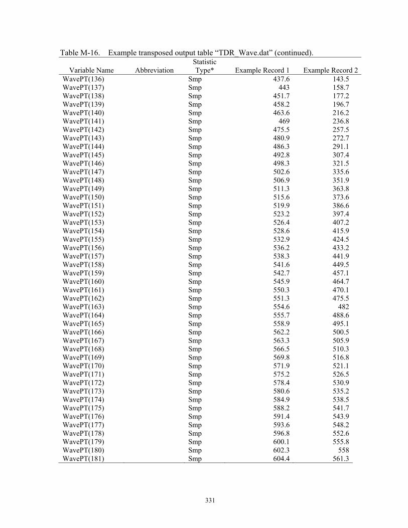
331



WavePT(136) Smp 437.6 143.5WavePT(137) Smp 443 158.7WavePT(138) Smp 451.7 177.2WavePT(139) Smp 458.2 196.7WavePT(140) Smp 463.6 216.2WavePT(141) Smp 469 236.8WavePT(142) Smp 475.5 257.5WavePT(143) Smp 480.9 272.7WavePT(144) Smp 486.3 291.1WavePT(145) Smp 492.8 307.4WavePT(146) Smp 498.3 321.5WavePT(147) Smp 502.6 335.6WavePT(148) Smp 506.9 351.9WavePT(149) Smp 511.3 363.8WavePT(150) Smp 515.6 373.6WavePT(151) Smp 519.9 386.6WavePT(152) Smp 523.2 397.4WavePT(153) Smp 526.4 407.2WavePT(154) Smp 528.6 415.9WavePT(155) Smp 532.9 424.5WavePT(156) Smp 536.2 433.2WavePT(157) Smp 538.3 441.9WavePT(158) Smp 541.6 449.5WavePT(159) Smp 542.7 457.1WavePT(160) Smp 545.9 464.7WavePT(161) Smp 550.3 470.1WavePT(162) Smp 551.3 475.5WavePT(163) Smp 554.6 482WavePT(164) Smp 555.7 488.6WavePT(165) Smp 558.9 495.1WavePT(166) Smp 562.2 500.5WavePT(167) Smp 563.3 505.9WavePT(168) Smp 566.5 510.3WavePT(169) Smp 569.8 516.8WavePT(170) Smp 571.9 521.1WavePT(171) Smp 575.2 526.5WavePT(172) Smp 578.4 530.9WavePT(173) Smp 580.6 535.2WavePT(174) Smp 584.9 538.5WavePT(175) Smp 588.2 541.7WavePT(176) Smp 591.4 543.9WavePT(177) Smp 593.6 548.2WavePT(178) Smp 596.8 552.6WavePT(179) Smp 600.1 555.8WavePT(180) Smp 602.3 558WavePT(181) Smp 604.4 561.3

332



WavePT(182) Smp 605.5 564.5WavePT(183) Smp 606.6 565.6WavePT(184) Smp 607.7 569.9WavePT(185) Smp 607.7 571WavePT(186) Smp 607.7 574.3WavePT(187) Smp 607.7 577.5WavePT(188) Smp 607.7 578.6WavePT(189) Smp 607.7 581.9WavePT(190) Smp 607.7 584WavePT(191) Smp 607.7 586.2WavePT(192) Smp 606.6 589.5WavePT(193) Smp 604.4 591.6WavePT(194) Smp 603.3 596WavePT(195) Smp 603.3 599.2WavePT(196) Smp 603.3 602.5WavePT(197) Smp 603.3 604.6WavePT(198) Smp 603.3 609WavePT(199) Smp 603.3 612.2WavePT(200) Smp 603.3 615.5WavePT(201) Smp 602.3 617.7WavePT(202) Smp 602.3 618.8WavePT(203) Smp 602.3 622WavePT(204) Smp 602.3 623.1WavePT(205) Smp 600.1 623.1WavePT(206) Smp 599 623.1WavePT(207) Smp 599 623.1WavePT(208) Smp 599 623.1WavePT(209) Smp 599 623.1WavePT(210) Smp 599 623.1WavePT(211) Smp 599 623.1WavePT(212) Smp 599 622WavePT(213) Smp 599 618.8WavePT(214) Smp 599 619.8WavePT(215) Smp 599 618.8WavePT(216) Smp 599 618.8WavePT(217) Smp 599 618.8WavePT(218) Smp 599 618.8WavePT(219) Smp 599 618.8WavePT(220) Smp 600.1 618.8WavePT(221) Smp 601.2 617.7WavePT(222) Smp 602.3 616.6WavePT(223) Smp 602.3 614.4WavePT(224) Smp 602.3 614.4WavePT(225) Smp 602.3 614.4WavePT(226) Smp 603.3 614.4WavePT(227) Smp 603.3 614.4

333



WavePT(228) Smp 603.3 614.4WavePT(229) Smp 603.3 614.4WavePT(230) Smp 603.3 614.4WavePT(231) Smp 603.3 614.4WavePT(232) Smp 603.3 614.4WavePT(233) Smp 605.5 614.4WavePT(234) Smp 604.4 614.4WavePT(235) Smp 605.5 613.3WavePT(236) Smp 606.6 613.3WavePT(237) Smp 606.6 613.3WavePT(238) Smp 606.6 613.3WavePT(239) Smp 607.7 613.3WavePT(240) Smp 607.7 613.3WavePT(241) Smp 607.7 613.3WavePT(242) Smp 608.8 614.4WavePT(243) Smp 610.9 614.4WavePT(244) Smp 610.9 614.4WavePT(245) Smp 610.9 614.4WavePT(246) Smp 610.9 614.4WavePT(247) Smp 610.9 614.4WavePT(248) Smp 612 614.4WavePT(249) Smp 612 614.4WavePT(250) Smp 612 616.6WavePT(251) Smp 612 617.7WavePT(252) Smp 612 617.7WavePT(253) Smp 612 617.7WavePT(254) Smp 612 618.8WavePT(255) Smp 612 618.8WavePT(256) Smp 612 618.8WavePT(257) Smp 612 618.8WavePT(258) Smp 614.2 618.8WavePT(259) Smp 615.3 619.8WavePT(260) Smp 616.4 622


334

Table M-19. Example transposed output table “TEData.dat”. Variable Name Abbreviation

StatisticType* Value Value

TIMESTAMP 4/3/2009 16:00 4/3/2009 17:00 RECORD RN 0 1 TE_sen(1) Smp 110209 110209 TE_sen(2) Smp 130209 130209 VWCm(1) Smp 0.069 0.068 VWCm(2) Smp 0.074 0.074 ECp(1) Smp 0.03 0.03 ECp(2) Smp 0.02 0.03 Temp(1) Smp 17.8 17.5 Temp(2) Smp 17.6 17.2


335

Table M-20. Example transposed output table “TPHP.dat”. Variable

Name Variable


Example Record 1

Example Record 2

TIMESTAMP TS 4/3/2009 16:00 4/3/2009 16:00 RECORD RN 0 1 sensorID Smp: 125003 125103 timer_1 Smp: 0 0 temp1_C_1 Smp: 13.62661 15.44885 temp1_mV_1 Smp: 0.3735516 0.3937925 temp2_C_1 Smp: 13.01524 14.12111 temp2_mv_1 Smp: 0.3667936 0.3790311 Vref1 Smp: 0.2940826 0.2933368 Vref2 Smp: 0.2927568 0.2923424 Vref3 Smp: 0.2924253 0.2919281 Vref4 Smp: 0.2923424 0.2917624 Vref5 Smp: 0.2920938 0.2916795 Vref6 Smp: 0.2920938 0.2915967 Vref7 Smp: 0.2919281 0.2915967 Vref8 Smp: 0.2919281 0.2915967 Power Smp: 900.6807 902.778 Vref Smp:avg 0.2924564 0.2919799 Rht Smp: 40 40.2 Rref Smp: 1.0014 1.0011 heat_time Smp:total 7.92 7.92 TPHP_out(20) diff temp_1 1 Smp 0.03599358 0.02086544 TPHP_out(21) diff temp_1 2 Smp 0.1019793 0.06557655 TPHP_out(22) diff temp_1 3 Smp 0.2203999 0.1579599 TPHP_out(23) diff temp_1 4 Smp 0.3941803 0.2950068 TPHP_out(24) diff temp_1 5 Smp 0.6067457 0.4692297 TPHP_out(25) diff temp_1 6 Smp 0.8340931 0.6582708 TPHP_out(26) diff temp_1 7 Smp 1.059759 0.8487234 TPHP_out(27) diff temp_1 8 Smp 1.267344 1.021268 TPHP_out(28) diff temp_1 9 Smp 1.44644 1.175918 TPHP_out(29) diff temp_1 10 Smp 1.598597 1.305259 TPHP_out(30) diff temp_1 11 Smp 1.71938 1.410794 TPHP_out(31) diff temp_1 12 Smp 1.813294 1.492543 TPHP_out(32) diff temp_1 13 Smp 1.881855 1.553475 TPHP_out(33) diff temp_1 14 Smp 1.929538 1.599542 TPHP_out(34) diff temp_1 15 Smp 1.95934 1.62926 TPHP_out(35) diff temp_1 16 Smp 1.972748 1.648578 TPHP_out(36) diff temp_1 17 Smp 1.972748 1.654525 TPHP_out(37) diff temp_1 18 Smp 1.96381 1.654525 TPHP_out(38) diff temp_1 19 Smp 1.945928 1.647092 TPHP_out(39) diff temp_1 20 Smp 1.920599 1.633718

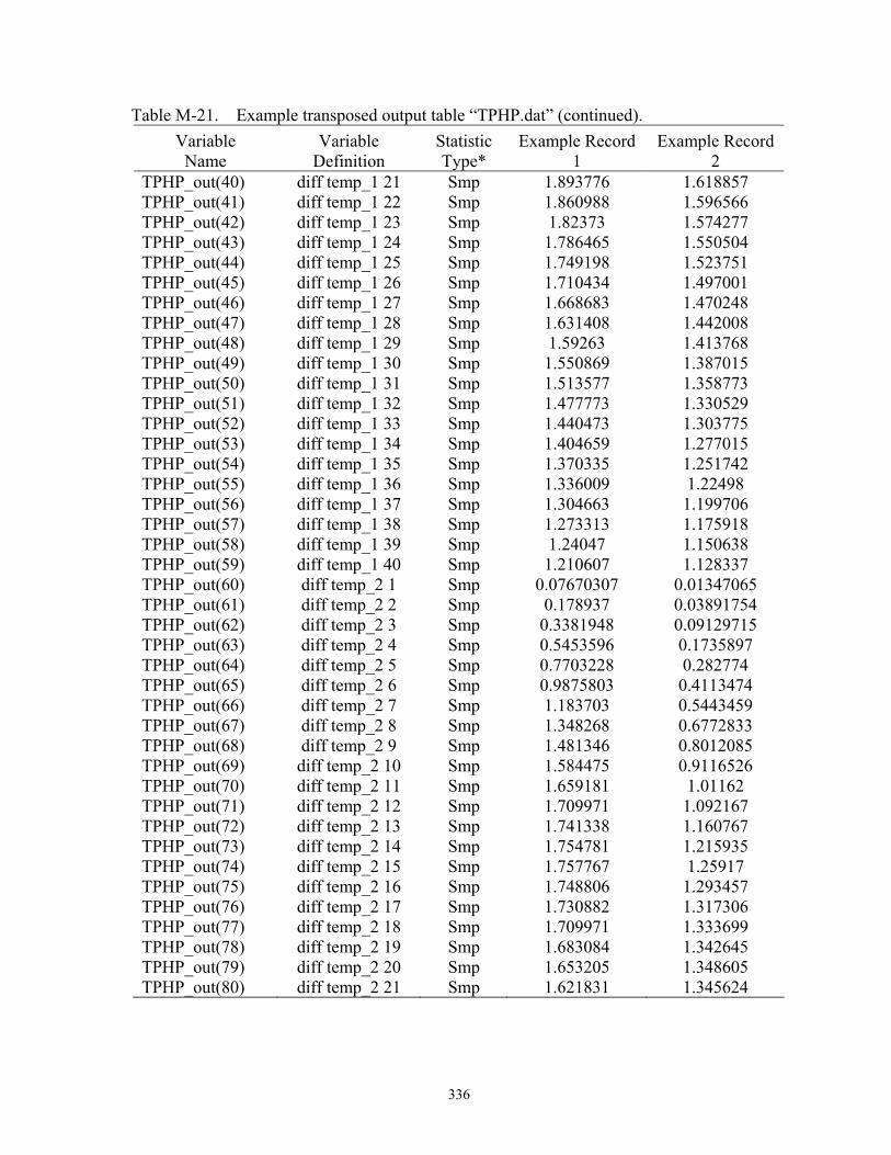
336

Table M-21. Example transposed output table “TPHP.dat” (continued). Variable

Name Variable


Example Record 1

Example Record 2

TPHP_out(40) diff temp_1 21 Smp 1.893776 1.618857 TPHP_out(41) diff temp_1 22 Smp 1.860988 1.596566 TPHP_out(42) diff temp_1 23 Smp 1.82373 1.574277 TPHP_out(43) diff temp_1 24 Smp 1.786465 1.550504 TPHP_out(44) diff temp_1 25 Smp 1.749198 1.523751 TPHP_out(45) diff temp_1 26 Smp 1.710434 1.497001 TPHP_out(46) diff temp_1 27 Smp 1.668683 1.470248 TPHP_out(47) diff temp_1 28 Smp 1.631408 1.442008 TPHP_out(48) diff temp_1 29 Smp 1.59263 1.413768 TPHP_out(49) diff temp_1 30 Smp 1.550869 1.387015 TPHP_out(50) diff temp_1 31 Smp 1.513577 1.358773 TPHP_out(51) diff temp_1 32 Smp 1.477773 1.330529 TPHP_out(52) diff temp_1 33 Smp 1.440473 1.303775 TPHP_out(53) diff temp_1 34 Smp 1.404659 1.277015 TPHP_out(54) diff temp_1 35 Smp 1.370335 1.251742 TPHP_out(55) diff temp_1 36 Smp 1.336009 1.22498 TPHP_out(56) diff temp_1 37 Smp 1.304663 1.199706 TPHP_out(57) diff temp_1 38 Smp 1.273313 1.175918 TPHP_out(58) diff temp_1 39 Smp 1.24047 1.150638 TPHP_out(59) diff temp_1 40 Smp 1.210607 1.128337 TPHP_out(60) diff temp_2 1 Smp 0.07670307 0.01347065 TPHP_out(61) diff temp_2 2 Smp 0.178937 0.03891754 TPHP_out(62) diff temp_2 3 Smp 0.3381948 0.09129715 TPHP_out(63) diff temp_2 4 Smp 0.5453596 0.1735897 TPHP_out(64) diff temp_2 5 Smp 0.7703228 0.282774 TPHP_out(65) diff temp_2 6 Smp 0.9875803 0.4113474 TPHP_out(66) diff temp_2 7 Smp 1.183703 0.5443459 TPHP_out(67) diff temp_2 8 Smp 1.348268 0.6772833 TPHP_out(68) diff temp_2 9 Smp 1.481346 0.8012085 TPHP_out(69) diff temp_2 10 Smp 1.584475 0.9116526 TPHP_out(70) diff temp_2 11 Smp 1.659181 1.01162 TPHP_out(71) diff temp_2 12 Smp 1.709971 1.092167 TPHP_out(72) diff temp_2 13 Smp 1.741338 1.160767 TPHP_out(73) diff temp_2 14 Smp 1.754781 1.215935 TPHP_out(74) diff temp_2 15 Smp 1.757767 1.25917 TPHP_out(75) diff temp_2 16 Smp 1.748806 1.293457 TPHP_out(76) diff temp_2 17 Smp 1.730882 1.317306 TPHP_out(77) diff temp_2 18 Smp 1.709971 1.333699 TPHP_out(78) diff temp_2 19 Smp 1.683084 1.342645 TPHP_out(79) diff temp_2 20 Smp 1.653205 1.348605 TPHP_out(80) diff temp_2 21 Smp 1.621831 1.345624

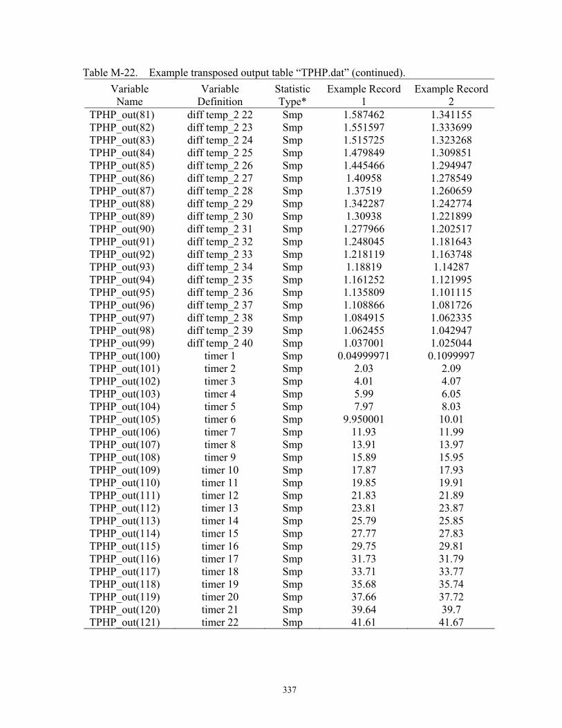
337


Name Variable


Example Record 1

Example Record 2

TPHP_out(81) diff temp_2 22 Smp 1.587462 1.341155 TPHP_out(82) diff temp_2 23 Smp 1.551597 1.333699 TPHP_out(83) diff temp_2 24 Smp 1.515725 1.323268 TPHP_out(84) diff temp_2 25 Smp 1.479849 1.309851 TPHP_out(85) diff temp_2 26 Smp 1.445466 1.294947 TPHP_out(86) diff temp_2 27 Smp 1.40958 1.278549 TPHP_out(87) diff temp_2 28 Smp 1.37519 1.260659 TPHP_out(88) diff temp_2 29 Smp 1.342287 1.242774 TPHP_out(89) diff temp_2 30 Smp 1.30938 1.221899 TPHP_out(90) diff temp_2 31 Smp 1.277966 1.202517 TPHP_out(91) diff temp_2 32 Smp 1.248045 1.181643 TPHP_out(92) diff temp_2 33 Smp 1.218119 1.163748 TPHP_out(93) diff temp_2 34 Smp 1.18819 1.14287 TPHP_out(94) diff temp_2 35 Smp 1.161252 1.121995 TPHP_out(95) diff temp_2 36 Smp 1.135809 1.101115 TPHP_out(96) diff temp_2 37 Smp 1.108866 1.081726 TPHP_out(97) diff temp_2 38 Smp 1.084915 1.062335 TPHP_out(98) diff temp_2 39 Smp 1.062455 1.042947 TPHP_out(99) diff temp_2 40 Smp 1.037001 1.025044 TPHP_out(100) timer 1 Smp 0.04999971 0.1099997 TPHP_out(101) timer 2 Smp 2.03 2.09 TPHP_out(102) timer 3 Smp 4.01 4.07 TPHP_out(103) timer 4 Smp 5.99 6.05 TPHP_out(104) timer 5 Smp 7.97 8.03 TPHP_out(105) timer 6 Smp 9.950001 10.01 TPHP_out(106) timer 7 Smp 11.93 11.99 TPHP_out(107) timer 8 Smp 13.91 13.97 TPHP_out(108) timer 9 Smp 15.89 15.95 TPHP_out(109) timer 10 Smp 17.87 17.93 TPHP_out(110) timer 11 Smp 19.85 19.91 TPHP_out(111) timer 12 Smp 21.83 21.89 TPHP_out(112) timer 13 Smp 23.81 23.87 TPHP_out(113) timer 14 Smp 25.79 25.85 TPHP_out(114) timer 15 Smp 27.77 27.83 TPHP_out(115) timer 16 Smp 29.75 29.81 TPHP_out(116) timer 17 Smp 31.73 31.79 TPHP_out(117) timer 18 Smp 33.71 33.77 TPHP_out(118) timer 19 Smp 35.68 35.74 TPHP_out(119) timer 20 Smp 37.66 37.72 TPHP_out(120) timer 21 Smp 39.64 39.7 TPHP_out(121) timer 22 Smp 41.61 41.67

338


Name Variable


Example Record 1

Example Record 2

TPHP_out(122) timer 23 Smp 43.59 43.65 TPHP_out(123) timer 24 Smp 45.57 45.63 TPHP_out(124) timer 25 Smp 47.55 47.61 TPHP_out(125) timer 26 Smp 49.53 49.59 TPHP_out(126) timer 27 Smp 51.5 51.56 TPHP_out(127) timer 28 Smp 53.48 53.54 TPHP_out(128) timer 29 Smp 55.46 55.52 TPHP_out(129) timer 30 Smp 57.44 57.5 TPHP_out(130) timer 31 Smp 59.41 59.47 TPHP_out(131) timer 32 Smp 61.39 61.45 TPHP_out(132) timer 33 Smp 63.37 63.43 TPHP_out(133) timer 34 Smp 65.35 65.41 TPHP_out(134) timer 35 Smp 67.33 67.39 TPHP_out(135) timer 36 Smp 69.31001 69.37 TPHP_out(136) timer 37 Smp 71.29 71.35 TPHP_out(137) timer 38 Smp 73.27 73.33 TPHP_out(138) timer 39 Smp 75.25 75.31001 TPHP_out(139) timer 40 Smp 77.23 77.29 TPHP_out(140) temp C_1 1 Smp 13.6626 15.46971 TPHP_out(141) temp C_1 2 Smp 13.72859 15.51442 TPHP_out(142) temp C_1 3 Smp 13.84701 15.60681 TPHP_out(143) temp C_1 4 Smp 14.02079 15.74385 TPHP_out(144) temp C_1 5 Smp 14.23335 15.91808 TPHP_out(145) temp C_1 6 Smp 14.4607 16.10712 TPHP_out(146) temp C_1 7 Smp 14.68637 16.29757 TPHP_out(147) temp C_1 8 Smp 14.89395 16.47012 TPHP_out(148) temp C_1 9 Smp 15.07305 16.62477 TPHP_out(149) temp C_1 10 Smp 15.22521 16.75411 TPHP_out(150) temp C_1 11 Smp 15.34599 16.85964 TPHP_out(151) temp C_1 12 Smp 15.4399 16.94139 TPHP_out(152) temp C_1 13 Smp 15.50846 17.00232 TPHP_out(153) temp C_1 14 Smp 15.55615 17.04839 TPHP_out(154) temp C_1 15 Smp 15.58595 17.07811 TPHP_out(155) temp C_1 16 Smp 15.59936 17.09743 TPHP_out(156) temp C_1 17 Smp 15.59936 17.10337 TPHP_out(157) temp C_1 18 Smp 15.59042 17.10337 TPHP_out(158) temp C_1 19 Smp 15.57254 17.09594 TPHP_out(159) temp C_1 20 Smp 15.54721 17.08257 TPHP_out(160) temp C_1 21 Smp 15.52038 17.06771 TPHP_out(161) temp C_1 22 Smp 15.4876 17.04541 TPHP_out(162) temp C_1 23 Smp 15.45034 17.02312

339


Name Variable


Example Record 1

Example Record 2

TPHP_out(163) temp C_1 24 Smp 15.41307 16.99935 TPHP_out(164) temp C_1 25 Smp 15.37581 16.9726 TPHP_out(165) temp C_1 26 Smp 15.33704 16.94585 TPHP_out(166) temp C_1 27 Smp 15.29529 16.9191 TPHP_out(167) temp C_1 28 Smp 15.25802 16.89086 TPHP_out(168) temp C_1 29 Smp 15.21924 16.86262 TPHP_out(169) temp C_1 30 Smp 15.17748 16.83586 TPHP_out(170) temp C_1 31 Smp 15.14019 16.80762 TPHP_out(171) temp C_1 32 Smp 15.10438 16.77938 TPHP_out(172) temp C_1 33 Smp 15.06708 16.75262 TPHP_out(173) temp C_1 34 Smp 15.03127 16.72586 TPHP_out(174) temp C_1 35 Smp 14.99694 16.70059 TPHP_out(175) temp C_1 36 Smp 14.96262 16.67383 TPHP_out(176) temp C_1 37 Smp 14.93127 16.64855 TPHP_out(177) temp C_1 38 Smp 14.89992 16.62477 TPHP_out(178) temp C_1 39 Smp 14.86708 16.59949 TPHP_out(179) temp C_1 40 Smp 14.83722 16.57718 TPHP_out(180) temp mV_1 1 Smp 0.3739501 0.394025 TPHP_out(181) temp mV_1 2 Smp 0.3746807 0.3945231 TPHP_out(182) temp mV_1 3 Smp 0.3759925 0.3955526 TPHP_out(183) temp mV_1 4 Smp 0.3779186 0.3970802 TPHP_out(184) temp mV_1 5 Smp 0.3802764 0.3990229 TPHP_out(185) temp mV_1 6 Smp 0.3828003 0.4011317 TPHP_out(186) temp mV_1 7 Smp 0.3853076 0.4032571 TPHP_out(187) temp mV_1 8 Smp 0.3876157 0.4051832 TPHP_out(188) temp mV_1 9 Smp 0.3896082 0.4069101 TPHP_out(189) temp mV_1 10 Smp 0.3913018 0.4083547 TPHP_out(190) temp mV_1 11 Smp 0.3926468 0.4095336 TPHP_out(191) temp mV_1 12 Smp 0.3936929 0.4104469 TPHP_out(192) temp mV_1 13 Smp 0.3944567 0.4111276 TPHP_out(193) temp mV_1 14 Smp 0.394988 0.4116424 TPHP_out(194) temp mV_1 15 Smp 0.3953201 0.4119745 TPHP_out(195) temp mV_1 16 Smp 0.3954696 0.4121903 TPHP_out(196) temp mV_1 17 Smp 0.3954696 0.4122567 TPHP_out(197) temp mV_1 18 Smp 0.3953699 0.4122567 TPHP_out(198) temp mV_1 19 Smp 0.3951707 0.4121737 TPHP_out(199) temp mV_1 20 Smp 0.3948884 0.4120243 TPHP_out(200) temp mV_1 21 Smp 0.3945895 0.4118582 TPHP_out(201) temp mV_1 22 Smp 0.3942242 0.4116091 TPHP_out(202) temp mV_1 23 Smp 0.3938091 0.4113601 TPHP_out(203) temp mV_1 24 Smp 0.393394 0.4110944

340


Name Variable


Example Record 1

Example Record 2

TPHP_out(204) temp mV_1 25 Smp 0.3929789 0.4107955 TPHP_out(205) temp mV_1 26 Smp 0.3925472 0.4104967 TPHP_out(206) temp mV_1 27 Smp 0.3920822 0.4101978 TPHP_out(207) temp mV_1 28 Smp 0.3916672 0.4098823 TPHP_out(208) temp mV_1 29 Smp 0.3912354 0.4095668 TPHP_out(209) temp mV_1 30 Smp 0.3907705 0.4092679 TPHP_out(210) temp mV_1 31 Smp 0.3903554 0.4089524 TPHP_out(211) temp mV_1 32 Smp 0.3899569 0.408637 TPHP_out(212) temp mV_1 33 Smp 0.3895418 0.4083381 TPHP_out(213) temp mV_1 34 Smp 0.3891433 0.4080392 TPHP_out(214) temp mV_1 35 Smp 0.3887613 0.4077569 TPHP_out(215) temp mV_1 36 Smp 0.3883795 0.407458 TPHP_out(216) temp mV_1 37 Smp 0.3880308 0.4071757 TPHP_out(217) temp mV_1 38 Smp 0.3876821 0.4069101 TPHP_out(218) temp mV_1 39 Smp 0.3873168 0.4066278 TPHP_out(219) temp mV_1 40 Smp 0.3869847 0.4063787 TPHP_out(220) temp C_2 1 Smp 13.09194 14.13458 TPHP_out(221) temp C_2 2 Smp 13.19417 14.16003 TPHP_out(222) temp C_2 3 Smp 13.35343 14.21241 TPHP_out(223) temp C_2 4 Smp 13.5606 14.2947 TPHP_out(224) temp C_2 5 Smp 13.78556 14.40388 TPHP_out(225) temp C_2 6 Smp 14.00282 14.53246 TPHP_out(226) temp C_2 7 Smp 14.19894 14.66545 TPHP_out(227) temp C_2 8 Smp 14.3635 14.79839 TPHP_out(228) temp C_2 9 Smp 14.49658 14.92232 TPHP_out(229) temp C_2 10 Smp 14.59971 15.03276 TPHP_out(230) temp C_2 11 Smp 14.67442 15.13273 TPHP_out(231) temp C_2 12 Smp 14.72521 15.21327 TPHP_out(232) temp C_2 13 Smp 14.75657 15.28187 TPHP_out(233) temp C_2 14 Smp 14.77002 15.33704 TPHP_out(234) temp C_2 15 Smp 14.773 15.38028 TPHP_out(235) temp C_2 16 Smp 14.76404 15.41457 TPHP_out(236) temp C_2 17 Smp 14.74612 15.43841 TPHP_out(237) temp C_2 18 Smp 14.72521 15.45481 TPHP_out(238) temp C_2 19 Smp 14.69832 15.46375 TPHP_out(239) temp C_2 20 Smp 14.66844 15.46971 TPHP_out(240) temp C_2 21 Smp 14.63707 15.46673 TPHP_out(241) temp C_2 22 Smp 14.6027 15.46226 TPHP_out(242) temp C_2 23 Smp 14.56683 15.45481 TPHP_out(243) temp C_2 24 Smp 14.53096 15.44438 TPHP_out(244) temp C_2 25 Smp 14.49508 15.43096

341


Name Variable


Example Record 1

Example Record 2

TPHP_out(245) temp C_2 26 Smp 14.4607 15.41605 TPHP_out(246) temp C_2 27 Smp 14.42482 15.39966 TPHP_out(247) temp C_2 28 Smp 14.39043 15.38177 TPHP_out(248) temp C_2 29 Smp 14.35752 15.36388 TPHP_out(249) temp C_2 30 Smp 14.32462 15.34301 TPHP_out(250) temp C_2 31 Smp 14.2932 15.32362 TPHP_out(251) temp C_2 32 Smp 14.26328 15.30275 TPHP_out(252) temp C_2 33 Smp 14.23335 15.28486 TPHP_out(253) temp C_2 34 Smp 14.20343 15.26398 TPHP_out(254) temp C_2 35 Smp 14.17649 15.2431 TPHP_out(255) temp C_2 36 Smp 14.15104 15.22222 TPHP_out(256) temp C_2 37 Smp 14.1241 15.20283 TPHP_out(257) temp C_2 38 Smp 14.10015 15.18344 TPHP_out(258) temp C_2 39 Smp 14.07769 15.16405 TPHP_out(259) temp C_2 40 Smp 14.05224 15.14615 TPHP_out(260) temp mV_2 1 Smp 0.3676404 0.3791806 TPHP_out(261) temp mV_2 2 Smp 0.3687695 0.3794628 TPHP_out(262) temp mV_2 3 Smp 0.3705296 0.380044 TPHP_out(263) temp mV_2 4 Smp 0.372821 0.3809572 TPHP_out(264) temp mV_2 5 Smp 0.3753117 0.3821694 TPHP_out(265) temp mV_2 6 Smp 0.3777193 0.3835973 TPHP_out(266) temp mV_2 7 Smp 0.3798946 0.3850752 TPHP_out(267) temp mV_2 8 Smp 0.381721 0.386553 TPHP_out(268) temp mV_2 9 Smp 0.3831989 0.3879311 TPHP_out(269) temp mV_2 10 Smp 0.3843445 0.3891599 TPHP_out(270) temp mV_2 11 Smp 0.3851748 0.3902724 TPHP_out(271) temp mV_2 12 Smp 0.3857393 0.391169 TPHP_out(272) temp mV_2 13 Smp 0.386088 0.3919328 TPHP_out(273) temp mV_2 14 Smp 0.3862375 0.3925472 TPHP_out(274) temp mV_2 15 Smp 0.3862707 0.3930287 TPHP_out(275) temp mV_2 16 Smp 0.386171 0.3934106 TPHP_out(276) temp mV_2 17 Smp 0.3859718 0.3936763 TPHP_out(277) temp mV_2 18 Smp 0.3857393 0.3938589 TPHP_out(278) temp mV_2 19 Smp 0.3854404 0.3939586 TPHP_out(279) temp mV_2 20 Smp 0.3851084 0.394025 TPHP_out(280) temp mV_2 21 Smp 0.3847597 0.3939918 TPHP_out(281) temp mV_2 22 Smp 0.3843778 0.393942 TPHP_out(282) temp mV_2 23 Smp 0.3839793 0.3938589 TPHP_out(283) temp mV_2 24 Smp 0.3835807 0.3937427 TPHP_out(284) temp mV_2 25 Smp 0.3831822 0.3935933 TPHP_out(285) temp mV_2 26 Smp 0.3828003 0.3934272

342


Name Variable


Example Record 1

Example Record 2

TPHP_out(286) temp mV_2 27 Smp 0.3824018 0.3932446 TPHP_out(287) temp mV_2 28 Smp 0.3820199 0.3930453 TPHP_out(288) temp mV_2 29 Smp 0.3816546 0.3928461 TPHP_out(289) temp mV_2 30 Smp 0.3812893 0.3926136 TPHP_out(290) temp mV_2 31 Smp 0.3809406 0.3923977 TPHP_out(291) temp mV_2 32 Smp 0.3806085 0.3921653 TPHP_out(292) temp mV_2 33 Smp 0.3802764 0.391966 TPHP_out(293) temp mV_2 34 Smp 0.3799444 0.3917336 TPHP_out(294) temp mV_2 35 Smp 0.3796455 0.3915011 TPHP_out(295) temp mV_2 36 Smp 0.3793632 0.3912686 TPHP_out(296) temp mV_2 37 Smp 0.3790643 0.3910528 TPHP_out(297) temp mV_2 38 Smp 0.3787987 0.3908369 TPHP_out(298) temp mV_2 39 Smp 0.3785496 0.3906211 TPHP_out(299) temp mV_2 40 Smp 0.3782673 0.3904218 TPHP_out(300) Smp 0 0 TPHP_out(301) Smp 0 0 TPHP_out(302) Smp 0 0

* Statistic types (Smp = sample, Smp:Avg = Average, Smp:Total = Total)

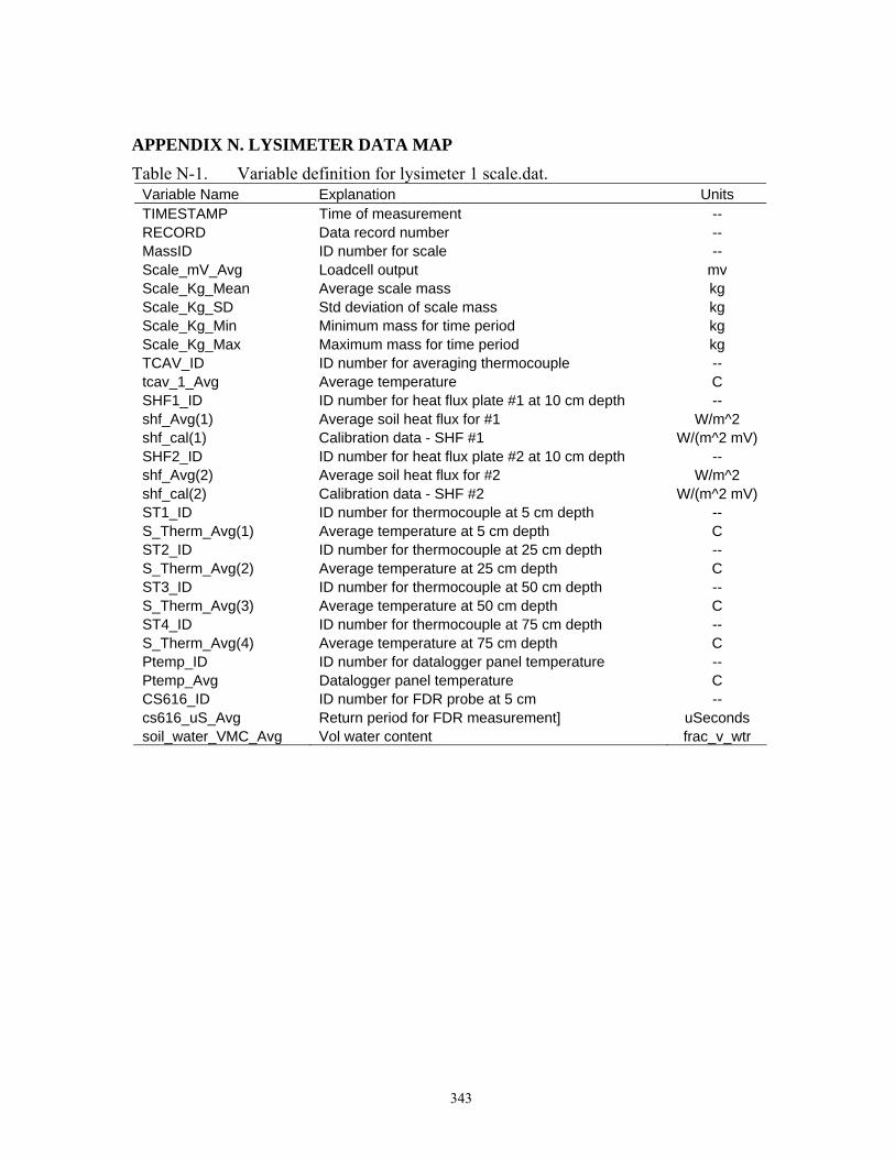
343

APPENDIX N. LYSIMETER DATA MAP Table N-1. Variable definition for lysimeter 1 scale.dat.

Variable Name Explanation Units TIMESTAMP Time of measurement -- RECORD Data record number -- MassID ID number for scale -- Scale_mV_Avg Loadcell output mv Scale_Kg_Mean Average scale mass kg Scale_Kg_SD Std deviation of scale mass kg Scale_Kg_Min Minimum mass for time period kg Scale_Kg_Max Maximum mass for time period kg TCAV_ID ID number for averaging thermocouple -- tcav_1_Avg Average temperature C SHF1_ID ID number for heat flux plate #1 at 10 cm depth -- shf_Avg(1) Average soil heat flux for #1 W/m^2 shf_cal(1) Calibration data - SHF #1 W/(m^2 mV) SHF2_ID ID number for heat flux plate #2 at 10 cm depth -- shf_Avg(2) Average soil heat flux for #2 W/m^2 shf_cal(2) Calibration data - SHF #2 W/(m^2 mV) ST1_ID ID number for thermocouple at 5 cm depth -- S_Therm_Avg(1) Average temperature at 5 cm depth C ST2_ID ID number for thermocouple at 25 cm depth -- S_Therm_Avg(2) Average temperature at 25 cm depth C ST3_ID ID number for thermocouple at 50 cm depth -- S_Therm_Avg(3) Average temperature at 50 cm depth C ST4_ID ID number for thermocouple at 75 cm depth -- S_Therm_Avg(4) Average temperature at 75 cm depth C Ptemp_ID ID number for datalogger panel temperature -- Ptemp_Avg Datalogger panel temperature C CS616_ID ID number for FDR probe at 5 cm -- cs616_uS_Avg Return period for FDR measurement] uSeconds soil_water_VMC_Avg Vol water content frac_v_wtr

344

Table N-2. Variable definition for lysimeter 2 scale.dat. Variable Name Explanation Units TIMESTAMP Time of measurement -- RECORD Data record number -- MassID ID number for scale -- Scale_mV_Avg Loadcell output mv Scale_Kg_Mean Average scale mass kg Scale_Kg_SD Std deviation of scale mass kg Scale_Kg_Min Minimum mass for time period kg Scale_Kg_Max Maximum mass for time period kg TCAV_ID ID number for averaging thermocouple -- tcav_1_Avg Average temperature C SHF1_ID ID number for heat flux plate #1 at 10 cm depth -- shf_Avg(1) Average soil heat flux for #1 W/m^2 shf_cal(1) Calibration data - SHF #1 W/(m^2 mV) SHF2_ID ID number for heat flux plate #2 at 10 cm depth -- shf_Avg(2) Average soil heat flux for #2 W/m^2 shf_cal(2) Calibration data - SHF #2 W/(m^2 mV) ST1_ID ID number for thermocouple at 5 cm depth -- S_Therm_Avg(1) Average temperature at 5 cm depth C ST2_ID ID number for thermocouple at 25 cm depth -- S_Therm_Avg(2) Average temperature at 25 cm depth C ST3_ID ID number for thermocouple at 50 cm depth -- S_Therm_Avg(3) Average temperature at 50 cm depth C ST4_ID ID number for thermocouple at 75 cm depth -- S_Therm_Avg(4) Average temperature at 75 cm depth C Ptemp_ID ID number for datalogger panel temperature -- Ptemp_Avg Datalogger panel temperature C

345

Table N-3. Variable definition for lysimeter 3 scale.dat. Variable Name Explanation Units TMSTAMP Time of measurement -- RECNBR Data record number -- MassID ID number for scale -- Scale_mV_Avg Loadcell output mv Scale_Kg_Mean Average scale mass kg Scale_Kg_SD Std deviation of scale mass kg Scale_Kg_Min Minimum mass for time period kg Scale_Kg_Max Maximum mass for time period kg TCAV_ID ID number for averaging thermocouple -- tcav_1_Avg Average temperature C SHF1_ID ID number for heat flux plate #1 at 10 cm depth -- shf_Avg(1) Average soil heat flux for #1 W/m^2

shf_cal(1) Calibration data - SHF #1 W/(m^2

mV) SHF2_ID ID number for heat flux plate #2 at 10 cm depth -- shf_Avg(2) Average soil heat flux for #2 W/m^2

shf_cal(2) Calibration data - SHF #2 W/(m^2

mV) ST1_ID ID number for thermocouple at 5 cm depth -- S_Therm_Avg(1) Average temperature at 5 cm depth C ST2_ID ID number for thermocouple at 25 cm depth -- S_Therm_Avg(2) Average temperature at 25 cm depth C ST3_ID ID number for thermocouple at 50 cm depth -- S_Therm_Avg(3) Average temperature at 50 cm depth C ST4_ID ID number for thermocouple at 75 cm depth -- S_Therm_Avg(4) Average temperature at 75 cm depth C Ptemp_ID ID number for datalogger panel temperature -- Ptemp_Avg Datalogger panel temperature C

Table N-4. Variable definition for lysimeter 1,2, and 3 tdr.dat.

Variable Name Explanation Units TMSTAMP Time of measurement -- RECNBR Data record number -- sensorID TDR probe ID --

LaL Ratio of apparent length to physical length (SQRT dielectric constant) --

ToppVWC Vol Water content using third order polynomial m3/m3TDR_EC Bulk electrical conductivity S/m a0 offset -- a1 coefficient A -- a2 coefficient B -- a3 coefficient C -- Note: theta = a0 + a1*(LaL)+a2*(LaL)^2+a3*(LaL)^3

346

Table N-5. Variable definition for lysimeter 1,2, and 3 hdu.dat. Variable Name Explanation Units TIMESTAMP Time of measurement -- RECORD Data record number -- sensorID HDU probe ID -- SoilTemp Initital soil temperature C deltaTemp Change in temperature from 0 - 30 seconds C T_1sec Temperature at 1 s C T_30sec Temperature at 30 s C RefTemp Panel T C Tstar Normalized change in temperature -- Psi Soil water potential Mpa wet deltaTemp for fully wetted probe C dry deltaTemp for very dry probe C alpha Calibration coefficient -- beta Calibration coefficient -- Note:HDU_Tstar = (HDU_dry(i)-del_T1(i))/(HDU_dry(i)-HDU_wet(i)) HDU_Psi = HDU_Tstar^(-1/HDU_beta(i))/HDU_alpha(i) If HDU_Tstar< 0, then HDU_Tstar= 1e-6

Table N-6. Definition of open path eddy covariance system (OPEC) sensors.

Sensors Definition CSAT3 three dimensional sonic anemometer LI-7500 open path infrared gas analyzer (CO2 and H2O) HMP45C temperature and relative humidity probe FW05 type E fine wire (0.0005 inch diameter) thermocouple CNR2 net radiometer HFP01SC soil heat flux plates (four sensors) TCAV type E thermocouple averaging soil temperature probes (two sensors) CS616 water content reflectometer (volumetric soil moisture)(two sensors)

Table N-7. Variable definition for BC_Eddy_dly.dat. Variable Name Explanation Units Equation TIMESTAMP Time of measurement -- -- RECORD Data record number -- --

Hs Sensible heat flux using sonic temperature W/m^2

H Sensible heat flux using hmp temperature

Fc_wpl Carbon dioxide flux (LI-7500), with Webb et al. term mg/(m^2 s)

LE_wpl Latent heat flux (LI-7500), with Webb et al. term W/m^2

Hc Sensible heat flux computed from Hs and LE_wpl W/m^2

tau Momentum flux kg/(m s^2) u_star Friction velocity m/s Ts_mean Air temperature C

stdev_Ts standard deviation of Air temperature C

cov_Ts_Ux

covariance of btwn air temperature and wind speed in x direction m C/s

cov_Ts_Uy

covariance of btwn air temperature and wind speed in y direction m C/s

cov_Ts_Uz

covariance of btwn air temperature and wind speed in z direction m C/s

co2_mean mean CO2 concentration mg/m^3

stdev_co2 standard deviation of CO2 concentration mg/m^3

cov_co2_Ux

covariance btwn CO2 concentration and wind speed in the x direction mg/(m^2 s)

347

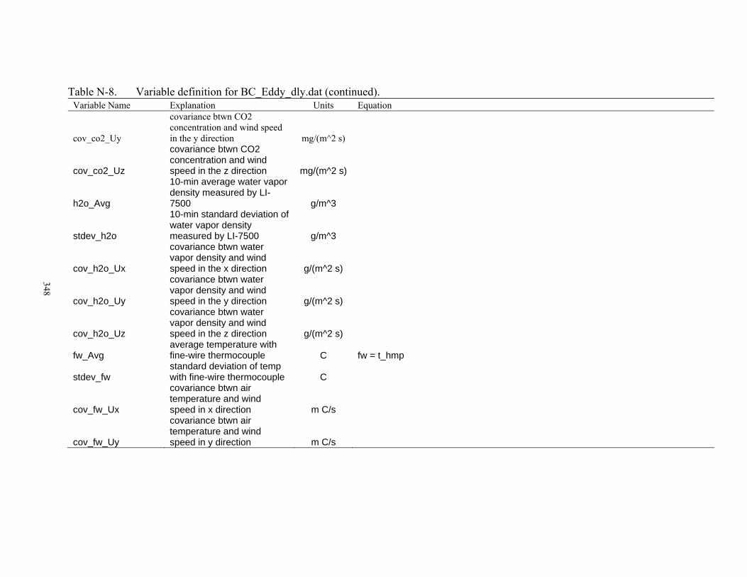
Table N-8. Variable definition for BC_Eddy_dly.dat (continued). Variable Name Explanation Units Equation

cov_co2_Uy

covariance btwn CO2 concentration and wind speed in the y direction mg/(m^2 s)

cov_co2_Uz

covariance btwn CO2 concentration and wind speed in the z direction mg/(m^2 s)

h2o_Avg

10-min average water vapor density measured by LI-7500 g/m^3

stdev_h2o

10-min standard deviation of water vapor density measured by LI-7500 g/m^3

cov_h2o_Ux

covariance btwn water vapor density and wind speed in the x direction g/(m^2 s)

cov_h2o_Uy

covariance btwn water vapor density and wind speed in the y direction g/(m^2 s)

cov_h2o_Uz

covariance btwn water vapor density and wind speed in the z direction g/(m^2 s)

fw_Avg average temperature with fine-wire thermocouple C fw = t_hmp

stdev_fw standard deviation of temp with fine-wire thermocouple C

cov_fw_Ux

covariance btwn air temperature and wind speed in x direction m C/s

cov_fw_Uy

covariance btwn air temperature and wind speed in y direction m C/s

348


cov_fw_Uz

covariance btwn air temperature and wind speed in z direction m C/s

Ux_Avg Average wind speed in the x direction m/s

stdev_Ux Standard deviation of wind speed in the x direction m/s

cov_Ux_Uy

Covariance btwn wind speed in the x and y directions (m/s)^2

cov_Ux_Uz

Covariance btwn wind speed in the x and z directions (m/s)^2

Uy_Avg Average wind speed in the y direction m/s

stdev_Uy Standard deviation of wind speed in the y direction m/s

cov_Uy_Uz

Covariance btwn wind speed in the y and z directions (m/s)^2

Uz_Avg Average wind speed in the z direction m/s

stdev_Uz Standard deviation of wind speed in the x direction m/s

press_mean Air pressure measured by LI-7500 kPa

t_hmp_mean Air temperature measured by HMP45C C

h2o_hmp_mean Mean HMP45C vapor density g/m^3 h2o_hmp_mean = e_hmp_mean/((t_hmp_mean+273.15)*RV)

rho_a_mean Mean air density kg/m^3

349

Table N-10. Variable definition for BC_Eddy_dly.dat (continued). Variable Name Explanation Units Equation wnd_dir_compass Wind direction degrees wnd_dir_compass = (wnd_dir_compass+CSAT3_AZIMUTH) MOD 360

wnd_dir_csat3

CSAT3 wind direction will be between 0 to 180 degrees and 0 to -180 degrees. degrees If ( wnd_dir_csat3 ) > 180 Then ( wnd_dir_csat3 = wnd_dir_csat3-360 )

wnd_spd wind speed measured by CSAT3 m/s

rslt_wnd_spd wind vector m/s WindVector (1,wnd_spd,wnd_dir_csat3,FP2,False,0,0,0) std_wnd_dir standard wind vector degrees

Fc_irga

Carbon dioxide flux (LI-7500), without Webb et al. term mg/(m^2 s) Fc_irga = cov_co2_Uz

LE_irga Latent heat flux (LI-7500), without Webb et al. term W/m^2 LE_irga = LV*cov_h2o_Uz

co2_wpl_LE LI-7500 Webb et al. term for carbon dioxide Eq. (24) mg/(m^2 s) co2_wpl_LE = MU_WPL*co2_mean/rho_d_mean*cov_h2o_Uz

co2_wpl_H LI-7500 Webb et al. term for carbon dioxide Eq. (24) mg/(m^2 s)

co2_wpl_H = (1+(MU_WPL*sigma_wpl))*co2_mean/(t_hmp_mean+273.15)*Hc/(rho_a_mean*CP)

h2o_wpl_LE LI-7500 Webb et al. term for water vapor Eq. (25) W/m^2

h2o_wpl_H = (1+(MU_WPL*sigma_wpl))*h2o_hmp_mean/(t_hmp_mean+273.15)*LV*cov_Ts_Uz

h2o_wpl_H LI-7500 Webb et al. term for water vapor Eq. (25) W/m^2 h2o_wpl_LE = MU_WPL*sigma_wpl*LE_irga

n_Tot Warnings collected during time period samples

csat_warnings Warnings collected during time period samples

irga_warnings Warnings collected during time period samples

del_T_f_Tot Warnings collected during time period samples

sig_lck_f_Tot Warnings collected during time period samples

350


amp_h_f_Tot Warnings collected during time period samples

amp_l_f_Tot Warnings collected during time period samples

chopper_f_Tot Warnings collected during time period samples

detector_f_Tot Warnings collected during time period samples

pll_f_Tot Warnings collected during time period samples

sync_f_Tot Warnings collected during time period samples

agc_Avg Automatic gain control unitless agc = INT ((diag_irga_work AND &h000f)*6.25+0.5) panel_temp_Avg Datalogger panel temperature C batt_volt_Avg Measure battery voltage V Rn_shortwave_Avg Shortwave CNR2 Net Radiation Measurements

Rn_Avg Average CNR2 Net Radiation Measurements W/m^2 Rn = Rn_shortwave+Rn_longwave

hfp01sc_1_Avg Average soil heat flux from HFP01SC soil heat flux plate 1 W/m^2




del_Tsoil(1) Change in soil temperature 1 C del_Tsoil(1) = Tsoil_avg(1)-prev_Tsoil(1) del_Tsoil(2) Change in soil temperature 2 C del_Tsoil(2) = Tsoil_avg(2)-prev_Tsoil(2)

soil_water_T_Avg(1)

CS616 Volumetric soil water content with temperature correction 1 frac_v_wtr soil_water_T(j) = -0.0663+cs616_T(j)*(-0.0063+cs616_T(j)*0.0007)

351


soil_water_T_Avg(2)

CS616 Volumetric soil water content with temperature correction 2 frac_v_wtr soil_water_T(j) = -0.0663+cs616_T(j)*(-0.0063+cs616_T(j)*0.0007)

Tsoil_avg(1) Average Soil Temperature from TCAV 1 C --

Tsoil_avg(2) Average Soil Temperature from TCAV 2 C --

cs616_wcr_Avg(1) CS616 soil water content probe 1 uSeconds --

cs616_wcr_Avg(2) CS616 soil water content probe 2 uSeconds --

par_totflx_Tot Total Flux measured by LI190SB PAR Sensor mmol/m^2 par_totflx = par_mV*par_mult_totflx

par_flxdens_Avg Flux Density measured by LI190SB PAR Sensor umol/s/m^2 par_flxdens = par_mV*par_mult_flxdens

wnd_spd_WVc(1) m/s wnd_spd_WVc(2) m/s wnd_spd_WVc(3) m/s wnd_spd_Max Maximum Wind Speed m/s wnd_spd_TMx m/s

Rain_mm_Tot

Total Rain measured by TE525/TE525WS Rain Gauge mm calibrated 4-30-08 by Brad Lyles 50.5 ml/10 tips => 0.108 mm/tip

Rn_longwave_Avg Longwave CNR2 Net Radiation Measurements

shf_cal(1) HFP01SC factory calibration 1

W/(m^2 mV)


W/(m^2 mV)


W/(m^2 mV)


W/(m^2 mV)

Note: The sign convention for the fluxes, except net radiation, is positive away from the surface and negative towards the surface.

352

353

APPENDIX O. NAMING CONVENTION FOR SENSOR NUMBER Data for each instrument is filed according to the sensor number: ‘WXY1Y2Z1Z2’. where, W: lysimeter number, 1 through 4, oriented south to north X: quadrant (NE, SE, SW, NW), 1 through 4, oriented clockwise beginning from

upper right quadrant or NE quadrant Y: depth of instrument Examples: 130505: Lysi 1, SW quad, 50 cm depth, SSS 211401: Lysi 2, NE quad, 250 cm depth, TDR 340303: Lysi 3, NW quad, 10 cm depth, TPHP Table O-1. Definition of sensor number.

W Lysimeter X Quadrant Y1Y2 Depth [cm] Z1Z2 Instrument

1 1 1 NE 01 0 01 TDR 2 2 2 SE 02 5 02 DPHP 3 3 3 SW 03 10 03 TPHP 4 4 4 NW 04 25 04 HDU

5 natural

soil 05 50 05 SSSS

06 60 06 Stherm 07 75 07 SHF 08 90 08 TCAV

09 100 09 ECH2O

10 140 10 SET 11 150 11 DTS Loops 12 190 12 DTS Pole 13 200 13 CS616 14 250 18 TC 15 290

16 300

354

An exception to this naming convention is the TPHP cluster or “Titanic” at 5 cm. To make the Sensor ID unique, the depth was ‘50’ for the highest TPHP and ‘53’ for the lowest. An example is given for lysimeter 1 in the table below. Table O-2. Sensor ID naming convention for TPHP cluster or "Titanic."

Sensor_ID Lysimeter Quadrant Depth Instrument 125003 1 SE Titanic 50 (highest) TPHP 125103 1 SE Titanic 51 TPHP 125203 1 SE Titanic 52 TPHP 125303 1 SE Titanic 53 (lowest) TPHP 110303 1 SW 10 TPHP 130303 1 SW 10 TPHP 110403 1 NW 25 TPHP 130403 1 NW 25 TPHP

Table O-3. Sensor ID naming convention for thermocouples (TC) located in natural soil

outside of lysimeter 3. Sensor_ID Lysimeter Quadrant Depth Instrument

520318 natural soil near SE corner of lysimeter 3 10 TC 520418 natural soil near SE corner of lysimeter 3 25 TC 520518 natural soil near SE corner of lysimeter 3 50 TC 520718 natural soil near SE corner of lysimeter 3 75 TC 520918 natural soil near SE corner of lysimeter 3 100 TC 521118 natural soil near SE corner of lysimeter 3 150 TC 521318 natural soil near SE corner of lysimeter 3 200 TC 521418 natural soil near SE corner of lysimeter 3 250 TC

521618 natural soil near SE corner of lysimeter 3 300 TC