1Atptmlttn

fumtodwaeTtca

trga

2Tt

wt

Alexander A. Kokhanovsky Vol. 24, No. 4 /April 2007 /J. Opt. Soc. Am. A 1131

Scattered light corrections to Sun photometry:analytical results for single and multiple

scattering regimes

Alexander A. Kokhanovsky

Institute of Remote Sensing, O. Hahn Allee 1, D-28334 Bremen, Germany

Received July 3, 2006; revised September 27, 2006; accepted November 3, 2006;posted November 10, 2006 (Doc. ID 72588); published March 14, 2007

Analytical equations for the diffused scattered light correction factor of Sun photometers are derived and ana-lyzed. It is shown that corrections are weakly dependent on the atmospheric optical thickness. They are influ-enced mostly by the size of aerosol particles encountered by sunlight on its way to a Sun photometer. In ad-dition, the accuracy of the small-angle approximation used in the work is studied with numerical calculationsbased on the exact radiative transfer equation. © 2007 Optical Society of America

OCIS codes: 010.0010, 010.1110, 010.1320.

as(

wTsde

wsldfaa

wtpW

w

aff

. INTRODUCTIONtmospheric optical thickness � is a crucial parameter

hat influences climate and weather. For clear skies, thisarameter is also a good indicator of atmospheric pollu-ion. The value of � for cloudless cases is determined byolecular and aerosol scattering and absorption. The mo-

ecular contribution is rather robust and can be sub-racted from the registered signal to yield the aerosol op-ical thickness �a, which is an important parameter for aumber of applications.On one hand, the measurements of � are quite straight-

orward. One must direct a photometer at the Sun andse the exponential attenuation law to determine the at-ospheric optical thickness. However, many complica-

ions arise, which often prevent the correct determinationf �. This includes the problem of the calibration (e.g., forifferent temperature regimes) and also the correctionith respect to the scattered light.1 A Sun photometer hasfinite field of view (FOV). Therefore, the scattered light

nters the instrument, increasing the registered signal.his leads to the underestimation of the derived opticalhickness if the results of measurements are not pro-essed correctly. This issue has been studied by manyuthors.2–6

The task of this work is to propose analytical equationshat can be used for the estimation of corresponding cor-ection factors both in single and multiple scattering re-imes, depending on the size of particles and also on thetmospheric optical thickness.

. SINGLE SCATTERING APPROXIMATIONhe power as received by a ground photometer looking inhe direction of the Sun can be expressed as7

F =��0

AId�, �1�

here A is the receiving cross section, d�=sin �d�d� ishe elementary solid angle, � is the zenith angle, � is the

1084-7529/07/041131-7/$15.00 © 2

zimuth, and I is the light intensity in the FOV of the in-trument defined by the solid angle �0. It follows from Eq.1) that

F = ���0

Id�, �2�

here the area � is a characteristic of a given instrument.he intensity as received by a photometer can be repre-ented as a sum of the direct light component Idir and theiffused intensity Idif. One can easily derive the followingxpression for the direct light intensity7:

Idir = E0 exp�− x����0 − ��, �3�

here ���0−�� is the delta function, x=� /�0, �0 is the co-ine of the incidence angle, � is the optical depth along theocal vertical, and E0 is the top-of-atmosphere solar irra-iance. It follows for the diffused light component in theramework of the single scattering approximation—ssuming that the zenith observation and incidencengles coincide7—

Idif =�0E0p��x exp�− x�

4, �4�

here �0=Ksca /Kext is the single scattering albedo, Ksca ishe scattering coefficient, Kext is the extinction coefficient,�� is the phase function, and is the scattering angle.e obtain from Eqs. (2)–(4) that

F = �E0 exp�− x��1 + fx�, �5�

here

f =�0

2 �0

0

p��sin d, �6�

nd 0 is the half-FOV angle. Taking into account thatx→0 for singly scattering media, we have approximatelyrom Eq. (5)

007 Optical Society of America

t�w

w

idst

=�vcvs

rmatpm

w

wh

d

w

Hftsi

wob

f

w

i

d=(trgTaa

FtsRtbe−

1132 J. Opt. Soc. Am. A/Vol. 24, No. 4 /April 2007 Alexander A. Kokhanovsky

F = �E0 exp�− �1 − f�x�; �7�

herefore, x= �1− f�−1x0, where x0=ln��E0 /F���0 /�0, and0 is the so-called apparent optical thickness. Also we canrite

� = C�0, �8�

here

C =1

1 − f�9�

s the correction factor (CF). Equations (8) and (9) wereerived by Shiobara and Asano2 in a way similar to thathown above and used for studies of diffuse light correc-ions to Sun photometry and pyrheliometry.6

Clearly, it follows that f=0 at 0=0 [see Eq. (6)] and ��0 then. In reality, 0�0, 0� f�1, and the true value ofis larger than the apparent optical thickness �0. C takesalues between approximately 1 and 2 for most practicalases, depending on the size of particles and the actualalue of the FOV angle.6 Even larger values of C are pos-ible if 0 is not small.

Let us estimate f for large spherical particles of radiusmuch larger than the wavelength �. Because 0→0 forodern spectrophotometers, we can use the following

pproximation8 for the normalized Mie intensity i�� inhe small-angle scattering region �→0� for a sphericalarticle of radius r and arbitrary complex refractive index:

i�� = 4

4�2� �, �10�

here =kr, k=2 /�, and

�� � =2J1� �

, �11�

here J1� � is the Bessel function. Equation (10) has aigh accuracy8 as →0, →�, and p�2�m−1� →�.The phase function of the spherical polydispersion is

efined as9

p�� =

2N�0

�

��r��i1 + i2�dr

k2Ksca, �12�

here ��r� is the particle size distribution (PSD) and

Ksca = N�0

�

r2��r�Qscadr. �13�

ere Qsca is the scattering efficiency factor determinedrom the Mie theory. The simple analytical expression forhe scaled phase function p̂��=�0p�� can be derived atmall angles using Eqs. (10)–(12) and also the fact that� i � i at small angles. So it follows that

1 2

p��� =2J1

2�kr�

2 , �14�

here we used the fact that Kext=2NM2 (M2 is the sec-nd moment of PSD) for large particles8 and angularrackets mean

y�kr� =

�0

�

y�kr�r2��r�dr

�0

�

r2��r�dr

�15�

or arbitrary function y�kr�. One obtains from Eq. (14) at=0 that

p��0� =k2M42

2, �16�

here M42�M4 /M2, and

Mn =�0

�

rn��r�dr �17�

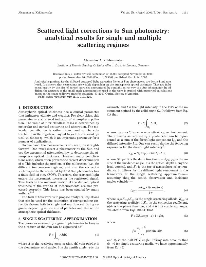
s the nth moment of PSD.The accuracy of calculations according to Eq. (14) is

emonstrated in Fig. 1 for the gamma PSD ��r�Br� exp�−�r /r0�, where B is the normalization constant

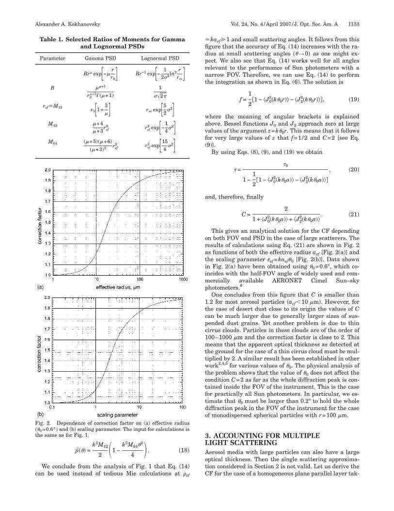
see Table 1), �=6, and r0 is the mode radius related tohe effective radius ref�M32 by the analytical equationef=r0�1+3/��. The values M32 and M42 [see Eq. (16)] areiven in Table 1 both for gamma and lognormal PSDs.he value of M62 shown in Table 1 appears in thesymptotic analysis of Eq. (14) as →0. That is, it followst small scattering angles that

ig. 1. Phase function of spherical polydispersions with effec-ive radius of 4, 6, 8, 10, and 12 �m [lower lines as →0 corre-pond to smaller particles (see Eq. (15) starting from aef=4 �m].esults obtained using Mie theory are shown by solid curves and

he approximation is given by dotted curves. Calculations haveeen performed for the gamma PSD with the half-width param-ter �=6 and �=0.5 �m. The complex refraction index m=1.520.008i was used in exact numerical calculations.

c

�fidprnt

wavf(

a

oratiimp

1tcpc1mttwtctftdo

3LAotC

F�t

Alexander A. Kokhanovsky Vol. 24, No. 4 /April 2007 /J. Opt. Soc. Am. A 1133

p��� =k2M42

2 �1 −k2M642

4 � . �18�

We conclude from the analysis of Fig. 1 that Eq. (14)an be used instead of tedious Mie calculations at

Table 1. Selected Ratios of Moments for Gammaand Lognormal PSDs

Parameter Gamma PSD Lognormal PSD

Br� exp�−�rr0 � Br−1 exp�− 1

2�2ln2r

rm �B ��+1

r0�+1���+1�

1

� 2

ref�M32 r0�1+3� � rm exp�5

2�2�

M42 �+4�+3

ref2 ref

2 exp�−14

�2�M64 ��+5���+6�

��+3�2 ref2 ref

2 exp�154

�2�

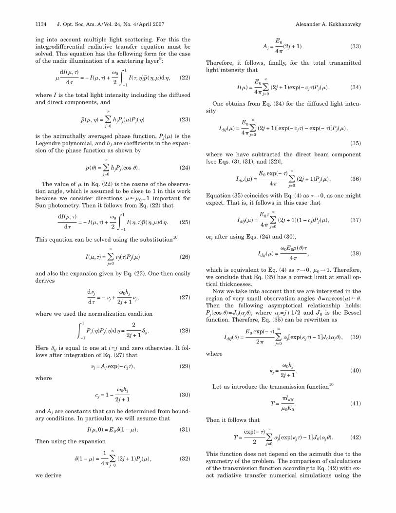
ig. 2. Dependence of correction factor on (a) effective radius0=0.6° � and (b) scaling parameter. The input for calculations ishe same as for Fig. 1.

ef

kaef�1 and small scattering angles. It follows from thisgure that the accuracy of Eq. (14) increases with the ra-ius at small scattering angles �→0� as one might ex-ect. We also see that Eq. (14) works well for all angleselevant to the performance of Sun photometers with aarrow FOV. Therefore, we can use Eq. (14) to performhe integration as shown in Eq. (6). The solution is

f =1

2�1 − J0

2�k0r� − J22�k0r��, �19�

here the meaning of angular brackets is explainedbove. Bessel functions J0 and J2 approach zero at largealues of the argument z=k0r. This means that it followsor very large values of z that f=1/2 and C=2 [see Eq.9)].

By using Eqs. (8), (9), and (19) we obtain

� =�0

1 −1

2�1 − J0

2�k0a� − J22�k0a��

, �20�

nd, therefore, finally

C =2

1 + J02�k0a� + J2

2�k0a�. �21�

This gives an analytical solution for the CF dependingn both FOV and PSD in the case of large scatterers. Theesults of calculations using Eq. (21) are shown in Fig. 2s functions of both the effective radius aef [Fig. 2(a)] andhe scaling parameter zef=kaef0 [Fig. 2(b)]. Data shownn Fig. 2(a) have been obtained using 0=0.6°, which co-ncides with the half-FOV angle of widely used and com-

ercially available AERONET Cimel Sun–skyhotometers.6

One concludes from this figure that C is smaller than.2 for most aerosol particles �aef�10 �m�. However, forhe case of desert dust close to its origin the values of Can be much larger due to generally larger sizes of sus-ended dust grains. Yet another problem is due to thinirrus clouds. Particles in these clouds are of the order of00–1000 �m and the correction factor is close to 2. Thiseans that the apparent optical thickness as detected at

he ground for the case of a thin cirrus cloud must be mul-iplied by 2. A similar result has been established in otherork2,4,5 for various values of 0. The physical analysis of

he problem shows that the value of 0 does not affect theondition C=2 as far as the whole diffraction peak is con-ained inside the FOV of the instrument. This is the caseor practically all Sun photometers. In particular, we es-imate that 0 must be larger than 0.2° to hold the wholeiffraction peak in the FOV of the instrument for the casef monodispersed spherical particles with r=100 �m.

. ACCOUNTING FOR MULTIPLEIGHT SCATTERINGerosol media with large particles can also have a largeptical thickness. Then the single scattering approxima-ion considered in Section 2 is not valid. Let us derive theF for the case of a homogeneous plane parallel layer tak-

iiso

wa

iLs

tbS

T

ad

w

Hl

w

aa

T

w

Tl

s

w[

Ee

o

wwt

rTPf

w

T

Tsoa

1134 J. Opt. Soc. Am. A/Vol. 24, No. 4 /April 2007 Alexander A. Kokhanovsky

ng into account multiple light scattering. For this thentegrodifferential radiative transfer equation must beolved. This equation has the following form for the casef the nadir illumination of a scattering layer9:

�dI��,��

d�= − I��,�� +

�0

2 �−1

1

I��,��p̄��,��d�, �22�

here I is the total light intensity including the diffusednd direct components, and

p̄��,�� = �j=0

�

hjPj���Pj��� �23�

s the azimuthally averaged phase function, Pj��� is theegendre polynomial, and hj are coefficients in the expan-ion of the phase function as shown by

p�� = �j=0

�

hjPj�cos �. �24�

The value of � in Eq. (22) is the cosine of the observa-ion angle, which is assumed to be close to 1 in this workecause we consider directions ���0=1 important forun photometry. Then it follows from Eq. (22) that

dI��,��

d�= − I��,�� +

�0

2 �−1

1

I��,��p̄��,��d�. �25�

his equation can be solved using the substitution10

I��,�� = �j=0

�

�j���Pj��� �26�

nd also the expansion given by Eq. (23). One then easilyerives

d�j

d�= − �j +

�0hj

2j + 1�j, �27�

here we used the normalization condition

�−1

1

Pi���Pj���d� =2

2j + 1�ij. �28�

ere �ij is equal to one at i= j and zero otherwise. It fol-ows after integration of Eq. (27) that

�j = Aj exp�− cj��, �29�

here

cj = 1 −�0hj

2j + 1�30�

nd Aj are constants that can be determined from bound-ry conditions. In particular, we will assume that

I��,0� = E0��1 − ��. �31�

hen using the expansion

��1 − �� =1

4�j=0

�

�2j + 1�Pj���, �32�

e derive

Aj =E0

4�2j + 1�. �33�

herefore, it follows, finally, for the total transmittedight intensity that

I��� =E0

4�j=0

�

�2j + 1�exp�− cj��Pj���. �34�

One obtains from Eq. (34) for the diffused light inten-ity

Idif��� =E0

4�j=0

�

�2j + 1��exp�− cj�� − exp�− ���Pj���,

�35�

here we have subtracted the direct beam componentsee Eqs. (3), (31), and (32)],

Idir��� =E0 exp�− ��

4 �j=0

�

�2j + 1�Pj���. �36�

quation (35) coincides with Eq. (4) as �→0, as one mightxpect. That is, it follows in this case that

Idif��� =E0�

4 �j=0

�

�2j + 1��1 − cj�Pj���, �37�

r, after using Eqs. (24) and (30),

Idif��� =�0E0p���

4, �38�

hich is equivalent to Eq. (4) as �→0, �0→1. Therefore,e conclude that Eq. (35) has a correct limit at small op-

ical thicknesses.Now we take into account that we are interested in the

egion of very small observation angles �=arccos����.hen the following asymptotical relationship holds:j�cos �=J0��j�, where �j= j+1/2 and J0 is the Bessel

unction. Therefore, Eq. (35) can be rewritten as

Idif�� =E0 exp�− ��

2 �j=0

�

�j�exp��j�� − 1�J0��j�, �39�

here

�j =�0hj

2j + 1. �40�

Let us introduce the transmission function10

T =Idif

�0E0. �41�

hen it follows that

T =exp�− ��

2 �j=0

�

�j�exp��j�� − 1�J0��j�. �42�

his function does not depend on the azimuth due to theymmetry of the problem. The comparison of calculationsf the transmission function according to Eq. (42) with ex-ct radiative transfer numerical simulations using the

vi�sTmIsa

tert(toefw

Ftca

Fpna

Fi

Alexander A. Kokhanovsky Vol. 24, No. 4 /April 2007 /J. Opt. Soc. Am. A 1135

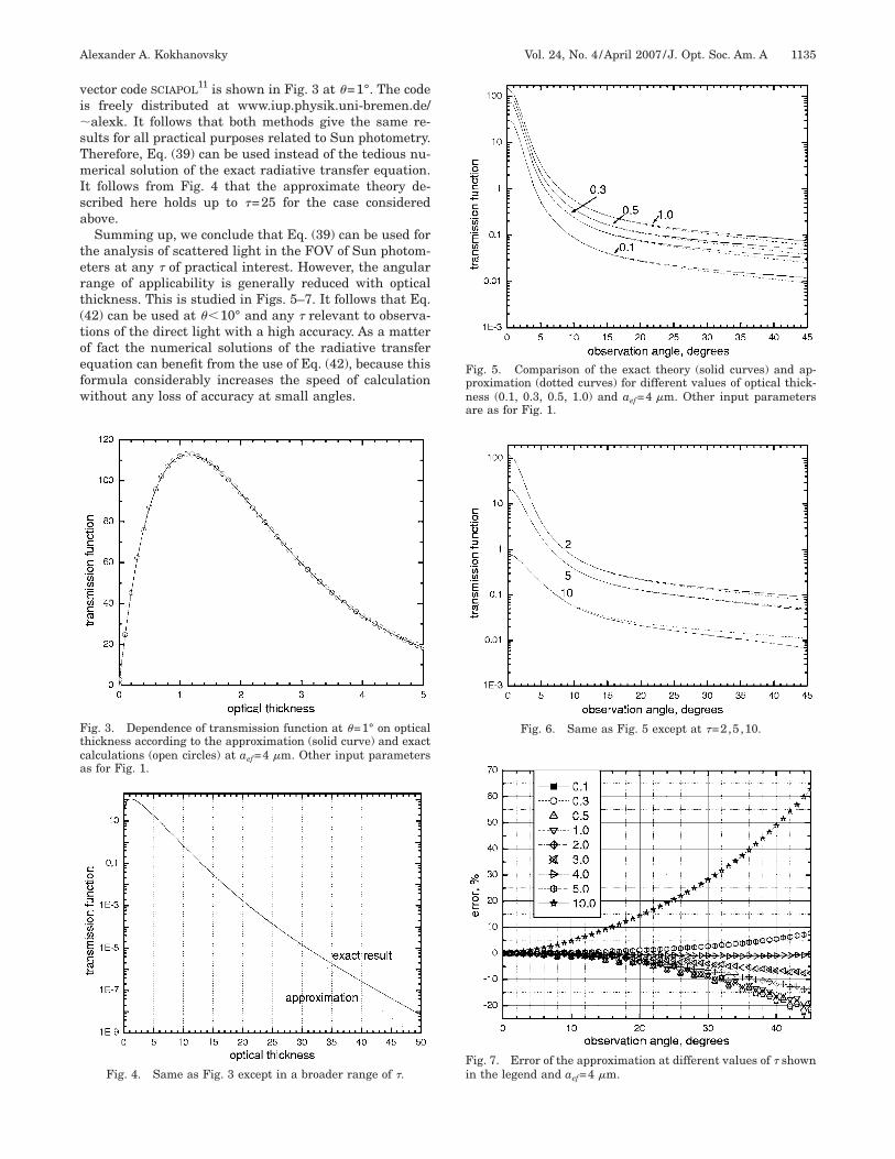
ector code SCIAPOL11 is shown in Fig. 3 at =1°. The codes freely distributed at www.iup.physik.uni-bremen.de/alexk. It follows that both methods give the same re-

ults for all practical purposes related to Sun photometry.herefore, Eq. (39) can be used instead of the tedious nu-erical solution of the exact radiative transfer equation.

t follows from Fig. 4 that the approximate theory de-cribed here holds up to �=25 for the case consideredbove.Summing up, we conclude that Eq. (39) can be used for

he analysis of scattered light in the FOV of Sun photom-ters at any � of practical interest. However, the angularange of applicability is generally reduced with opticalhickness. This is studied in Figs. 5–7. It follows that Eq.42) can be used at �10° and any � relevant to observa-ions of the direct light with a high accuracy. As a matterf fact the numerical solutions of the radiative transferquation can benefit from the use of Eq. (42), because thisormula considerably increases the speed of calculationithout any loss of accuracy at small angles.

ig. 3. Dependence of transmission function at =1° on opticalhickness according to the approximation (solid curve) and exactalculations (open circles) at aef=4 �m. Other input parameterss for Fig. 1.

Fig. 4. Same as Fig. 3 except in a broader range of �.

ig. 5. Comparison of the exact theory (solid curves) and ap-roximation (dotted curves) for different values of optical thick-ess (0.1, 0.3, 0.5, 1.0) and aef=4 �m. Other input parametersre as for Fig. 1.

Fig. 6. Same as Fig. 5 except at �=2,5,10.

ig. 7. Error of the approximation at different values of � shownn the legend and a =4 �m.

ef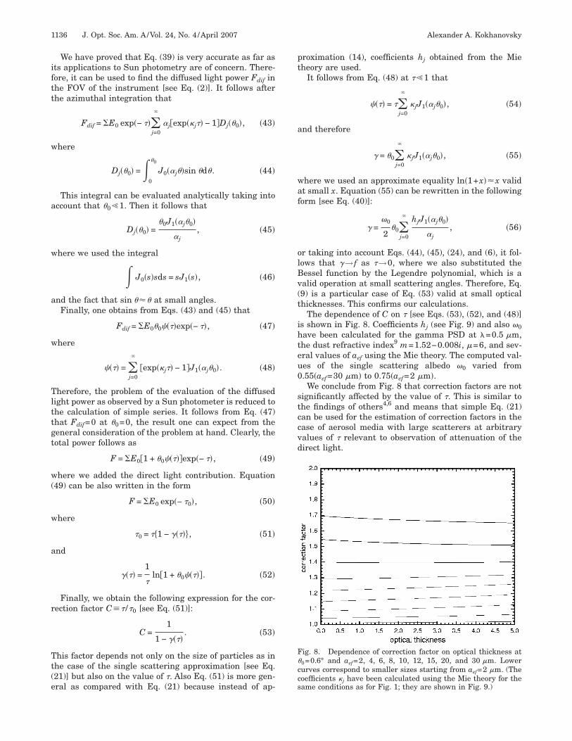

iftt

w

a

w

a

w

Tlttgt

w(

w

a

r

Tt(e

pt

a

waf

olBv(t

ihteu0

stccvd

Fccs

1136 J. Opt. Soc. Am. A/Vol. 24, No. 4 /April 2007 Alexander A. Kokhanovsky

We have proved that Eq. (39) is very accurate as far asts applications to Sun photometry are of concern. There-ore, it can be used to find the diffused light power Fdif inhe FOV of the instrument [see Eq. (2)]. It follows afterhe azimuthal integration that

Fdif = �E0 exp�− ���j=0

�

�j�exp��j�� − 1�Dj�0�, �43�

here

Dj�0� =�0

0

J0��j�sin d. �44�

This integral can be evaluated analytically taking intoccount that 0�1. Then it follows that

Dj�0� =0J1��j0�

�j, �45�

here we used the integral

� J0�s�sds = sJ1�s�, �46�

nd the fact that sin � at small angles.Finally, one obtains from Eqs. (43) and (45) that

Fdif = �E00����exp�− ��, �47�

here

���� = �j=0

�

�exp��j�� − 1�J1��j0�. �48�

herefore, the problem of the evaluation of the diffusedight power as observed by a Sun photometer is reduced tohe calculation of simple series. It follows from Eq. (47)hat Fdif=0 at 0=0, the result one can expect from theeneral consideration of the problem at hand. Clearly, theotal power follows as

F = �E0�1 + 0�����exp�− ��, �49�

here we added the direct light contribution. Equation49) can be also written in the form

F = �E0 exp�− �0�, �50�

here

�0 = ��1 − �����, �51�

nd

���� =1

�ln�1 + 0�����. �52�

Finally, we obtain the following expression for the cor-ection factor C�� /�0 [see Eq. (51)]:

C =1

1 − ����. �53�

his factor depends not only on the size of particles as inhe case of the single scattering approximation [see Eq.21)] but also on the value of �. Also Eq. (51) is more gen-ral as compared with Eq. (21) because instead of ap-

roximation (14), coefficients hj obtained from the Mieheory are used.

It follows from Eq. (48) at ��1 that

���� = ��j=0

�

�jJ1��j0�, �54�

nd therefore

� = 0�j=0

�

�jJ1��j0�, �55�

here we used an approximate equality ln�1+x��x validt small x. Equation (55) can be rewritten in the followingorm [see Eq. (40)]:

� =�0

20�

j=0

� hjJ1��j0�

�j, �56�

r taking into account Eqs. (44), (45), (24), and (6), it fol-ows that �→ f as �→0, where we also substituted theessel function by the Legendre polynomial, which is aalid operation at small scattering angles. Therefore, Eq.9) is a particular case of Eq. (53) valid at small opticalhicknesses. This confirms our calculations.

The dependence of C on � [see Eqs. (53), (52), and (48)]s shown in Fig. 8. Coefficients hj (see Fig. 9) and also �0ave been calculated for the gamma PSD at �=0.5 �m,he dust refractive index9 m=1.52−0.008i, �=6, and sev-ral values of aef using the Mie theory. The computed val-es of the single scattering albedo �0 varied from.55�aef=30 �m� to 0.75�aef=2 �m�.We conclude from Fig. 8 that correction factors are not

ignificantly affected by the value of �. This is similar tohe findings of others4,6 and means that simple Eq. (21)an be used for the estimation of correction factors in thease of aerosol media with large scatterers at arbitraryalues of � relevant to observation of attenuation of theirect light.

ig. 8. Dependence of correction factor on optical thickness at0=0.6° and aef=2, 4, 6, 8, 10, 12, 15, 20, and 30 �m. Lowerurves correspond to smaller sizes starting from aef=2 �m. (Theoefficients �j have been calculated using the Mie theory for theame conditions as for Fig. 1; they are shown in Fig. 9.)

nesmcEaplccfeswEacps

4WlcmTpi

Ttsct

kf

jlotemts

prTit

tces

b

R

1

1

1

1

Fc

Alexander A. Kokhanovsky Vol. 24, No. 4 /April 2007 /J. Opt. Soc. Am. A 1137

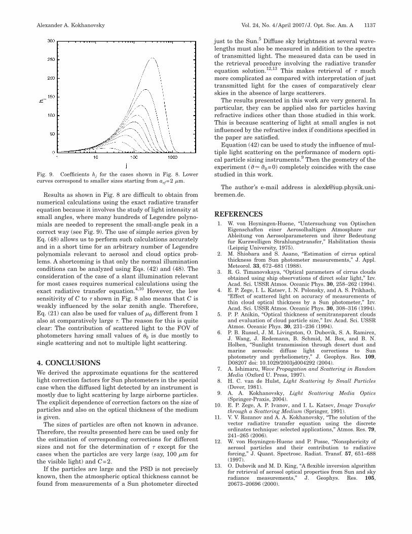
Results as shown in Fig. 8 are difficult to obtain fromumerical calculations using the exact radiative transferquation because it involves the study of light intensity atmall angles, where many hundreds of Legendre polyno-ials are needed to represent the small-angle peak in a

orrect way (see Fig. 9). The use of simple series given byq. (48) allows us to perform such calculations accuratelynd in a short time for an arbitrary number of Legendreolynomials relevant to aerosol and cloud optics prob-ems. A shortcoming is that only the normal illuminationonditions can be analyzed using Eqs. (42) and (48). Theonsideration of the case of a slant illumination relevantor most cases requires numerical calculations using thexact radiative transfer equation.4,10 However, the lowensitivity of C to � shown in Fig. 8 also means that C iseakly influenced by the solar zenith angle. Therefore,q. (21) can also be used for values of �0 different from 1lso at comparatively large �. The reason for this is quitelear: The contribution of scattered light to the FOV ofhotometers having small values of 0 is due mostly toingle scattering and not to multiple light scattering.

. CONCLUSIONSe derived the approximate equations for the scattered

ight correction factors for Sun photometers in the specialase when the diffused light detected by an instrument isostly due to light scattering by large airborne particles.he explicit dependence of correction factors on the size ofarticles and also on the optical thickness of the mediums given.

The sizes of particles are often not known in advance.herefore, the results presented here can be used only forhe estimation of corresponding corrections for differentizes and not for the determination of � except for theases when the particles are very large (say, 100 �m forhe visible light) and C=2.

If the particles are large and the PSD is not preciselynown, then the atmospheric optical thickness cannot be

ig. 9. Coefficients hj for the cases shown in Fig. 8. Lowerurves correspond to smaller sizes starting from aef=2 �m.

ound from measurements of a Sun photometer directed

ust to the Sun.5 Diffuse sky brightness at several wave-engths must also be measured in addition to the spectraf transmitted light. The measured data can be used inhe retrieval procedure involving the radiative transferquation solution.12,13 This makes retrieval of � muchore complicated as compared with interpretation of just

ransmitted light for the cases of comparatively clearkies in the absence of large scatterers.

The results presented in this work are very general. Inarticular, they can be applied also for particles havingefractive indices other than those studied in this work.his is because scattering of light at small angles is not

nfluenced by the refractive index if conditions specified inhe paper are satisfied.

Equation (42) can be used to study the influence of mul-iple light scattering on the performance of modern opti-al particle sizing instruments.9 Then the geometry of thexperiment ����0=0� completely coincides with the casetudied in this work.

The author’s e-mail address is alexk@iup.physik.uni-remen.de.

EFERENCES1. W. von Hoyningen-Huene, “Untersuchung von Optischen

Eigenschaften einer Aerosolhaltigen Atmosphare zurAbleitung von Aerosolparameteren und ihrer Bedeutungfur Kurzwelligen Strahlungstransfer,” Habilitation thesis(Leipzig University, 1975).

2. M. Shiobara and S. Asano, “Estimation of cirrus opticalthickness from Sun photometer measurements,” J. Appl.Meteorol. 33, 672–681 (1988).

3. R. G. Timanovskaya, “Optical parameters of cirrus cloudsobtained using ship observations of direct solar light,” Izv.Acad. Sci. USSR Atmos. Oceanic Phys. 30, 258–262 (1994).

4. E. P. Zege, I. L. Katsev, I. N. Polonsky, and A. S. Prikhach,“Effect of scattered light on accuracy of measurements ofthin cloud optical thickness by a Sun photometer,” Izv.Acad. Sci. USSR Atmos. Oceanic Phys. 30, 308–316 (1994).

5. P. P. Anikin, “Optical thickness of semitransparent cloudsand evaluation of cloud particle size,” Izv. Acad. Sci. USSRAtmos. Oceanic Phys. 30, 231–236 (1994).

6. P. B. Russel, J. M. Livingston, O. Dubovik, S. A. Ramirez,J. Wang, J. Redemann, B. Schmid, M. Box, and B. N.Holben, “Sunlight transmission through desert dust andmarine aerosols: diffuse light corrections to Sunphotometry and pyrheliometry,” J. Geophys. Res. 109,D08207 doi: 10.1029/2003jd004292 (2004).

7. A. Ishimaru, Wave Propagation and Scattering in RandomMedia (Oxford U. Press, 1997).

8. H. C. van de Hulst, Light Scattering by Small Particles(Dover, 1981).

9. A. A. Kokhanovsky, Light Scattering Media Optics(Springer-Praxis, 2004).

0. E. P. Zege, A. P. Ivanov, and I. L. Katsev, Image Transferthrough a Scattering Medium (Springer, 1991).

1. V. V. Rozanov and A. A. Kokhanovsky, “The solution of thevector radiative transfer equation using the discreteordinates technique: selected applications,” Atmos. Res. 79,241–265 (2006).

2. W. von Hoyningen-Huene and P. Posse, “Nonsphericity ofaerosol particles and their contribution to radiativeforcing,” J. Quant. Spectrosc. Radiat. Transf. 57, 651–688(1997).

3. O. Dubovik and M. D. King, “A flexible inversion algorithmfor retrieval of aerosol optical properties from Sun and skyradiance measurements,” J. Geophys. Res. 105,

20673–20696 (2000).