Scattered Node Compact Finite

Difference-Type Formulas Generated from

Radial Basis Functions

Grady B. Wright a,∗,1, Bengt Fornberg b,2

aDepartment of Mathematics, University of Utah, Salt Lake City, UT 84112-0090,

USA

bDepartment of Applied Mathematics, University of Colorado, Boulder, CO

80309-0526, USA

Abstract

In standard equispaced finite difference (FD) formulas, symmetries can make theorder of accuracy relatively high compared to the number of nodes in the FD stencil.With scattered nodes, such symmetries are no longer available. The generalization ofcompact FD formulas that we propose for scattered nodes and radial basis functions(RBFs) achieves the goal of still keeping the number of stencil nodes small withouta similar reduction in accuracy. We analyze the accuracy of these new compactRBF-FD formulas by applying them to some model problems, and study the effectsof the shape parameter that arises in, for example, the multiquadric radial function.

Key words: Radial basis functions, partial differential equations, finite differencemethod, compact, Mehrstellenverfahren, mesh-free1991 MSC: 41A21, 41A30, 41A63, 65D25, 65N06

1 Introduction

Radial basis functions (RBFs) are a primary tool for interpolating multidi-mensional scattered data. In the past decade or so they have also received

∗ Corresponding author.Email addresses: wright@math.utah.edu (Grady B. Wright ),

fornberg@colorado.edu (Bengt Fornberg).1 The work was supported by NSF VIGRE grant DMS-0091675.2 The work was supported by NSF grants DMS-9810751 (VIGRE) and DMS-0309803.

Preprint submitted to Elsevier Science

increased attention as a “mesh-free” method for numerically solving partialdifferential equations (PDEs) on irregular domains by a global collocationapproach (see, for example, [1–4]). While these methods can be spectrally ac-curate (when proper attention is paid to boundaries), they generally result inhaving to solve a large, ill-conditioned, dense linear system. Some attemptshave been made to resolve this problem [3,5,6] (and the references therein).However, stability issues have limited the use of RBFs for time dependentproblems and adapting the methods for non-linear equations has proven to bedifficult. To combat all of these problems, a “local” method has recently beenproposed that gives up spectral accuracy for a sparse, better-conditioned linearsystem and more flexibility for handling non-linearities. This new “mesh-free”method is essentially a generalization of the classical finite difference (FD)method to scattered node layouts and appears to have been investigated in-dependently by Shu et al. [7,8], Tolstykh et al. [9], Cecil et al. [10], and thepresent authors [11].

In its most general form, the FD method consists of approximating somederivative of a function u at a given point based on a linear combination ofthe value of u at some surrounding nodes. In the classical 1-D case, u is givenat n equispaced nodes, xin

i=1, and the kth derivative of u, at say x = xj

(1 ≤ j ≤ n), is approximated by the FD formula

dku

dxk

∣∣∣∣∣x=xj

= u(k)(xj) ≈n∑

i=1

ckj,iu(xi) , (1)

where ckj,i are called the FD weights and are usually computed using polyno-mial interpolation [12,13]. These 1-D formulas can be combined to create FDformulas for partial derivatives in two and higher dimensions. This strategy,however, requires that the nodes of the stencils are situated on some kind ofstructured grid (or collection of structured grids), which severely limits thegeometric flexibility of the FD method.

One obvious approach for bypassing this problem is to instead allow the nodesof the FD stencil to be placed freely, so that a good discretization of the phys-ical domain can be obtained. However, this approach also raises the questionof how the weights of the scattered node FD formulas should be computed.Abgrall [14] and Schonauer and Adolph [15], for example, propose extend-ing the classical polynomial interpolation technique. This idea, however, hasnot become widely used, partly because it leads to several ambiguities abouthow to generate the FD formulas. For example, what mixed terms should beincluded in the multivariate polynomial interpolant to the nodes, and howshould a set of nodes that leads to a singular polynomial interpolation prob-lem be handled (polynomial interpolation in > 1-D is not well-posed [16]). Allof these ambiguities can be resolved if RBF interpolation is instead used togenerate the weights in the FD formula [7,9–11].

2

An RBF interpolant is formed by taking a linear combination of translatesof a single univariate basis function φ(r) that is radially symmetric aboutits center. Thus, no decisions need to be made about what mixed terms toinclude in the interpolant. Moreover, for the appropriate choice of φ(r), theRBF interpolation method is well-posed in all dimensions. The following aresome other properties that make RBF interpolants an attractive choice:

• Since the only geometric property used by an RBF interpolant is the pair-wise distances between points, higher dimensions do not increase the codingcomplexity associated with computing the interpolants.

• RBF interpolants can be very accurate at approximating derivatives [17,18].• Certain types of radial functions φ(r) feature a “shape” parameter that

allows them to vary from being nearly flat to sharply peaked. Recently ithas been shown [19–22] that, under some mild restrictions on φ(r), theRBF interpolants converge to polynomial interpolants in the limit of φ(r)becoming entirely flat. Thus, all classical FD formulas can be recovered bythe limiting RBF interpolant (when the nodes are arranged accordingly).

We refer to this method of using RBF interpolants to generate the weights ofa FD formula as the RBF-FD method.

One of the issues with using scattered node FD formulas (whether the weightsare generated by polynomials or RBFs) is that symmetries cannot be exploitedto increase the accuracy of the formulas. Thus, the number of nodes in thestencils tend to be relatively large compared to the resulting accuracy. Tocircumvent this problem, we propose a generalization of a method introducedby Collatz [23] under the name Mehrstellenverfahren, and later developed intocompact FD formulas by Lele [24]. The basic idea behind this method is to keepthe stencil size fixed and to also include in the FD formula a linear combinationof derivatives of u at surrounding nodes. For example, the accuracy of the 1-Dformula (1) can be increased with a formula of the form

dku

dxk

∣∣∣∣∣x=xj

= u(k)(xj) ≈n∑

i=1

i6=j

ckj,iu(k)(xi) +

n∑

i=1

ckj,iu(xi) . (2)

In the case of 1-D and equispaced nodes, the weights ckj,i and ckj,i can be con-veniently derived using Pade approximants [13]. For scattered nodes, and forRBFs, this Pade approach is no longer available. Instead, we propose a methodbased on Hermite RBF interpolation. We refer to our proposed compact FDmethod as the RBF-HFD method.

The remainder of the paper is structured as follows: In Section 2, we reviewsome properties of the standard and Hermite RBF interpolation methods andintroduce some closed form expressions for the cardinal RBF interpolants,which prove valuable for deriving the RBF-FD and HFD formulas in Section

3

3. In Section 4, we study the effect of the shape parameter on the RBF-FD andHFD formulas. In particular, we are interested in how the formulas behave inthe limit of flat radial functions. In Section 5, we illustrate the effectivenessof the RBF-HFD formulas for solving some elliptic PDEs and discuss variousimplementation details. We conclude with some remarks in Section 6.

2 RBF interpolation

Since the RBF-FD formulas are obtained from RBF interpolants, we reviewin this section some properties of RBF interpolation. We discuss standardRBF interpolation in which only function values are specified. This forms thebackground for Hermite RBF interpolation, in which function and derivativevalues are specified.

2.1 Standard RBF interpolation

Given a set of distinct nodes xi ∈ Rd, i = 1, . . . , n, and corresponding (scalar)

function values u(xi), i = 1, . . . , n, the standard RBF interpolation problemis to find an interpolant of the form

s(x) =n∑

i=1

λi φ(‖x− xi‖) +m∑

j=1

βjpj(x), (3)

where φ(r) is some radial function, ‖ · ‖ is the standard Euclidean norm,and pk(x)m

k=1 is a basis for the space of all d-variate polynomials that havedegree ≤ Q. The expansion coefficients λi and βj are determined by enforcingthe conditions

s(xi) = u(xi), i = 1, . . . , n, and (4)n∑

i=1

λipj(xi) = 0, j = 1, . . . , m. (5)

The degree of the augmented polynomial in (3) depends on φ(r) and its inclu-sion may be necessary to guarantee a well-posed interpolation problem [25].Table 1 lists a few of the many available choices for φ(r).

In this study, we are primarily interested in the infinitely smooth radial func-tions since, by suitable choices of the shape parameter ε, they can providemore accurate interpolants than the piecewise smooth case [26,27]. We post-pone the discussion on the effect of ε until Section 4. For now, we assume itis fixed at some non-zero value.

4

Type of basis function φ(r)

Piecewise smooth RBFs

Generalized Duchon spline r2k log r, k ∈ N, or

r2ν , ν > 0 and ν 6∈ N

Wendland (1 − r)k+p(r), p a polynomial, k ∈ N

Infinitely smooth RBFs

Gaussian (GA) e−(εr)2

Generalized multiquadric (1 + (εr)2)ν/2, ν 6= 0 and ν 6∈ 2N

• Multiquadric (MQ) (1 + (εr)2)1/2

• Inverse multiquadric (IMQ) (1 + (εr)2)−1/2

• Inverse quadratic (IQ) (1 + (εr)2)−1

Table 1Some commonly used radial basis functions. Note: in all cases, ε > 0.

Although (3) is well-posed without any polynomial augmentation for the GA,MQ, IMQ, and IQ RBFs in Table 1, we set Q = 0 (i.e. m = 1) in orderto impose the condition that the RBF-FD formulas are exact for constants.Thus, the standard RBF interpolant that we consider has the form

s(x) =n∑

i=1

λi φ(‖x− xi‖) + β , (6)

Imposing the conditions (4) and (5) leads to the symmetric, block linear systemof equations [

Φ eeT 0

]

︸ ︷︷ ︸A

[λ

β

]=

[u0

], (7)

where Φi,j = φ(‖xi − xj‖), i, j = 1, . . . , n, and ei = 1, i = 1, . . . , n.

When deriving RBF-FD formulas in Section 3, we make use of the Lagrangeform the RBF interpolant (6):

s(x) =n∑

i=1

ψi(x)u(xi) , (8)

where ψi(x) are of the form (6) and satisfy the cardinal conditions

ψi(xk) =

1 if k = i

0 if k 6= i, k = 1, . . . , n . (9)

There turns out to be a nice closed-form expression for ψi(x) that first ap-peared in [20]. Denote by Ak(x), k = 1, . . . , n, the matrix A in (7) with the

5

8x

x9

x2

x7

x6

x10

x3

1

x4

x

x5

Fig. 1. Example of a scattered node Hermite interpolation problem.

kth row replaced by the vector

B(x) =[φ(‖x− x1‖) φ(‖x− x2‖) · · · φ(‖x− xn‖) 1

]. (10)

Note that with this notation A = Ak(xk).

Theorem 1 ([20]) The cardinal RBF interpolant of the form (6) that satis-fies (9) is given by

ψi(x) =det (Ai(x))

det (A). (11)

While (11) is not recommended for computational work, it is useful for ana-lytically studying the effects of the shape parameter ε in Section 4.

2.2 Hermite RBF interpolation

Let L be some linear differential operator (e.g., the Laplacian, L = ∆) and letσ be a vector containing some combination ofm ≤ n distinct numbers from theset 1, . . . , n. Then the Hermite interpolation problem we consider is to find afunction s(x) that interpolates u(x) at the distinct nodes xi, i = 1, . . . , n, andinterpolates Lu(x) at xσj

, j = 1, . . . , m. To clarify the notation, suppose u isgiven at the nodes x1, x2, . . . , x10 in Figure 1 and Lu is given at the nodes withdouble circles (i.e. x2, x4, x5, x6, x10). Then using the notation of the problemn = 10, m = 5, and σ = 2, 4, 5, 6, 10.

Solutions to this Hermite problem with RBFs have been around since Hardy’sintroduction of the MQ method [28] (see also [29]). Other expositions on thisand related Hermite-type RBF problems can be found, for example, in [30–32]. The Hermite RBF method we will use is similar to the Hermite-Birkhoffmethod proposed by Wu [32]. The idea is to introduce m more unknowns

6

to (6) in order to satisfy the m new interpolation conditions. Formally, theinterpolant takes the form

s(x) =n∑

i=1

λiφ(‖x− xi‖) +m∑

j=1

αjL2φ(‖x− xσj‖) + β , (12)

where

L2φ(‖x− xj‖) := Lφ(‖x− y‖)∣∣∣y=xj

,

i.e. L acts on φ as a function of the second variable y. For the remainder ofthis article we will also use the notation

Lφ(‖xj − y‖) = L1φ(‖xj − y‖) := Lφ(‖x− y‖)∣∣∣x=xj

,

i.e. if L or L1 act on φ, then the operator applies to the first variable. Forexample, if d = 1 and L = d

dxthen L2φ(‖x − xj‖) = −L1φ(‖x − xj‖) =

−Lφ(‖x− xj‖).

Imposing the interpolation conditions (4), (5), and

Ls(xσj) = Lu(xσj

), j = 1, . . . , m, (13)

leads to the following block linear system of equations

Φ ΦL2 eΦL1 ΦL1L2 0eT 0T 0

︸ ︷︷ ︸AH

λ

α

β

=

uLu0

, (14)

where Φ and e are given by (7) and

ΦL2

i,j = L2φ(‖xi − xσj‖) , i = 1, . . . , n, j = 1, . . . , m,

ΦL1

i,j = L1φ(‖xσi− xj‖) , i = 1, . . . , m, j = 1, . . . , n,

ΦL1L2

i,j = L1[L2φ(‖xσi− xσj

‖)] , i = 1, . . . , m, j = 1, . . . , m,

Note that by using L1 and L2 in defining (14), we have the relationship ΦL1 =(ΦL2)T , making AH symmetric. For the appropriate choice of φ, AH is alsoguaranteed to be non-singular [31].

We can also express (12) in the following Lagrange form:

s(x) =n∑

i=1

ψi(x)u(xi) +m∑

j=1

ψσj(x)Lu(xσj

) , (15)

7

where ψi(x) and ψσj(x) are of the form (12) and satisfy the cardinal conditions

ψi(xk) =

1 if k = i

0 if k 6= i, k = 1, . . . , n , (16)

Lψi(xσk) = 0 , k = 1, . . . , m , (17)

and

ψσj(xk) = 0 , k = 1, . . . , n , (18)

Lψσj(xσk

) =

1 if k = j

0 if k 6= j, k = 1, . . . , m . (19)

Like the standard RBF interpolation case, there turns out to be a nice closed-form expression for ψi(x) and ψσj

(x). Denote AHk (x), k = 1, . . . , n+m, as the

matrix AH in (14) with the kth row replaced by the vector

BH(x) =[B(x) L2φ(‖x− xσ1

‖) · · · L2φ(‖x− xσm‖) 1

], (20)

where B(x) is given by (10), but without the last entry.

Theorem 2 Let ψi(x) and ψσj(x) be of the form (12) and satisfy the condi-

tions (16),(17) and (18),(19). Then, provided the matrix AH in (14) is non-singular,

ψi(x) =det

(AH

i (x))

det (AH), (21)

and

ψσj(x) =

det(AH

n+j(x))

det (AH), (22)

PROOF. The result follows by using the same inspection argument givenin [20] for proving Theorem 1.

We postpone the discussion of the consequences of this formula as it relatesto the shape parameter ε until Section 4.

3 RBF-FD Formulation

In this section we describe how the RBF-FD and HFD formulas are generated.With out loss of generality, we consider a stencil consisting of n (scattered)

8

nodes x1, . . . , xn and are interested in approximating Lu(x1), for some lineardifferential operator L.

3.1 RBF-FD method

The goal is to find weights ci such that,

Lu(x1) ≈n∑

i=1

ciu(xi) . (23)

For example, given the 1-D scattered node stencil

x4

x3

x1

x2

x5

,

we look for an approximation of the form

Lu(x1) ≈5∑

i=1

ciu(xi) ,

or in computational molecule form

Lu(x1) ≈ c4 c3 c1 c2 c5 u .

(24)

Using the Lagrange form of the standard RBF interpolant (8) to approximateu(x) and then applying L gives

Lu(x1) ≈ Ls(x1) =n∑

i=1

Lψi(x1)u(xi) .

Thus, the weights in RBF-FD formula (23) are formally given by

ci = Lψi(x1) .

In practice, the weights are computed by solving the linear system

A[c|µ]T = (LB(x1))T , (25)

where A is the matrix in (7), B(x) is the row vector (10), and µ is a (scalar)dummy value related to the constant β in (6). Note that the constraint (5)enforces the condition

n∑

i=1

ci = 0 ,

9

i.e. the RBF-FD stencil is exact for all constants.

3.2 RBF-HFD method

The goal now is to increase the accuracy of the approximation (23) withoutincreasing the stencil size by using nodes where u and Lu are given exactly.Let σ be a vector containing some combination of m < n distinct numbersfrom the set 2, . . . , n, then we seek to find weights ci and cσj

such that

Lu(x1) ≈m∑

j=1

cσjLu(xσj

) +n∑

i=1

ciu(xi) . (26)

For example, suppose we wish to increase the accuracy of the 1-D example(24) from the previous section by including values of Lu(x3) and Lu(x5), i.e.using the stencil

x4

x3

x1

x2

x5 ,

where a single circle indicates that the value of u is used at that node, anda double circle indicates that the values of u and Lu are used. Then we letm = 2, σ = 3, 5, and look for an approximation of the form

Lu(x1) ≈ c3 c5 Lu+

c4 c3 c1 c2 c5 u .

The Hermite interpolation example in Figure 1 can alternatively be viewed asan example of a 2-D compact scattered node stencil with n = 10, m = 5 andσ = 2, 4, 5, 6, 10.

Using the Lagrange form of the Hermite RBF interpolant (15) to approximateu(x) and then applying L gives

Lu(x1) ≈ Ls(x1) =n∑

i=1

Lψi(x1)u(xi) +m∑

j=1

Lψσj(x1)Lu(xσj

) .

Thus, the weights in the RBF-HFD formula (26) are formally given by

ci = Lψi(x1) and cσj= Lψσj

(x1) .

In practice, the weights are computed by solving the linear system

AH[c|c|µ]T = (LBH(x1))T , (27)

10

where AH is the matrix in (14), BH(x) is the row vector (20), and µ is a dummy(scalar) value related to the constant β in (12). Like the standard RBF-FDformula, the constraint (5) enforces that (26) is exact for all constants.

Note that the above formulation for computing compact FD formulas differsfrom the standard polynomial-based formulation. For polynomials, the pointat which we are constructing the approximation about does not matter; theonly thing that does matter is that the formulas are exact for as high a degreepolynomial as possible [13].

4 Observations on the effect of the shape parameter ε

In this section, we make some observations with regard to ε on the RBF-FD and HFD formulas. We are primarily interested in studying the resultingformulas as we let ε → 0.

4.1 Some theoretical results on the ε → 0 limit

For nodes in 1-D, it was first shown in [19] that, under some mild restrictionson the infinitely smooth radial functions φ(r) (e.g. MQ, see Table 1), thestandard RBF interpolant converges to the Lagrange interpolating polynomialas ε → 0. This result means that all “classical”polynomial-based FD stencilsare reproduced by the standard RBF-FD stencils (with the appropriate choiceof φ(r)) in the limit of ε → 0. A few examples of this result are given in thenext section.

For nodes in two and higher dimensions, the situation is complicated by thefact that multivariate polynomial interpolation is not well-posed [16]. Whilethe standard RBF interpolant typically converges to a low degree multivariatepolynomial as ε → 0, there are circumstances where the interpolant mayinstead diverge; see [20–22,33,34] for more details. The authors are unaware ofany similar study of limiting (ε→ 0) Hermite RBF interpolants. However, weexpect similar results to those of the standard RBF interpolant. For example,the following theorem indicates that polynomial type results may be expectedin the ε→ 0 limit.

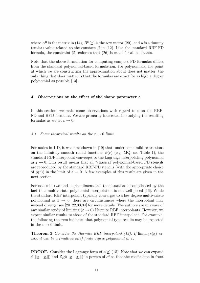
Theorem 3 Consider the Hermite RBF interpolant (12). If limε→0 s(x) ex-ists, it will be a (multivariate) finite degree polynomial in x.

PROOF. Consider the Lagrange form of s(x) (15). Note that we can expandφ(‖x− xi‖) and L2φ(‖x− xi‖) in powers of ε2 so that the coefficients in front

11

of these powers will be some polynomial in x. The same will, therefore, holdfor the determinant in the numerator of (21) and (22). Thus, the ratios in (21)and (22) will be of the respective forms

ψi(x) =ε2pipoly in x + ε2pi+2poly in x + · · ·ε2qiconstant + ε2qi+2constant + · · ·

and

ψσj(x) =

ε2pjpoly in x + ε2pj+2poly in x + · · ·ε2qjconstant + ε2qj+2constant + · · ·

,

where pi, qi, pj , and qj are positive integers. Since ψi(xi) = 1 and Lψσj(xσj

) =1, it is impossible to have pi > qi and pj > qj . If pi < qi or pj < qj , the limitfails to exist. Thus, when pi = qi and pj = qj, s(x) is some polynomial in x.

Like the polynomial result for the standard RBF interpolant, we can use The-orem 3 to conclude that when the underlying Hermite interpolant exists, theRBF-HFD formulas will be exact for some polynomials. In the next two sec-tions, we give a few examples that demonstrate this result.

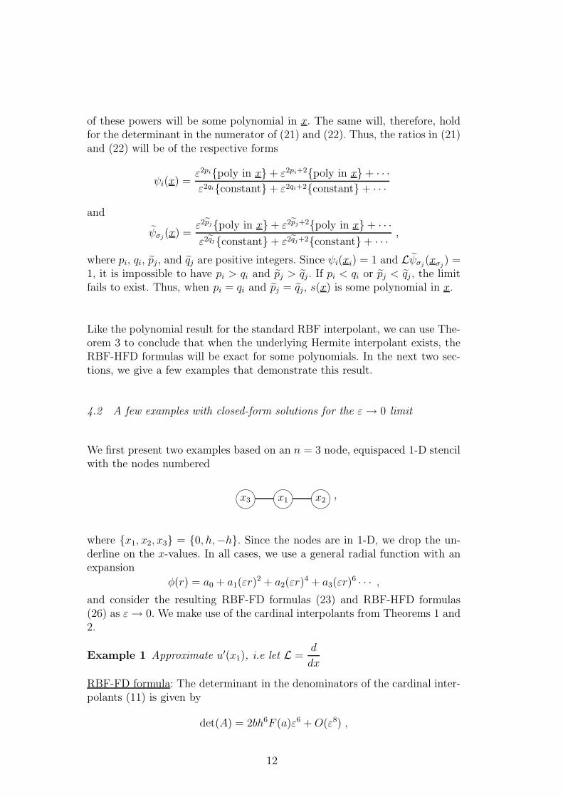
4.2 A few examples with closed-form solutions for the ε → 0 limit

We first present two examples based on an n = 3 node, equispaced 1-D stencilwith the nodes numbered

x3

x1

x2

,

where x1, x2, x3 = 0, h,−h. Since the nodes are in 1-D, we drop the un-derline on the x-values. In all cases, we use a general radial function with anexpansion

φ(r) = a0 + a1(εr)2 + a2(εr)

4 + a3(εr)6 · · · ,

and consider the resulting RBF-FD formulas (23) and RBF-HFD formulas(26) as ε→ 0. We make use of the cardinal interpolants from Theorems 1 and2.

Example 1 Approximate u′(x1), i.e let L =d

dx

RBF-FD formula: The determinant in the denominators of the cardinal inter-polants (11) is given by

det(A) = 2bh6F (a)ε6 +O(ε8) ,

12

while the determinants in the numerators are given by

det(A1(x)) = −2bh4(x− h)(x+ h)F (a)ε6 +O(ε8),

det(A2(x)) = bh4x(x+ h)F (a)ε6 +O(ε8),

det(A3(x)) = bh4x(x− h)F (a)ε6 +O(ε8) ,

where b = 24 and

F (a) = a1a2 . (28)

As expected from [19], provided a1a2 6= 0, ψi(x), i = 1, 2, 3, converge to thestandard cardinal interpolating polynomials in the limit as ε → 0. Thus, theclassical, centered, second order FD formula for u′(x1) is recovered in the ε → 0limit.

RBF-HFD formula: Using the notation from Section 2.2 and 3.2, we let m = 2and σ = 2, 3, i.e.

x3

x1

x2

.

The determinant in the denominators of the cardinal interpolants (21) and(22) is given by

det(AH) = 4bh16F (a)ε20 +O(ε22) , (29)

while the determinants in the numerators are given by

det(AH1 (x)) = −4bh12(x2 − h2)2F (a)ε20 +O(ε22) ,

det(AH2 (x)) = bh12(2x− 3h)x(x+ h)2F (a)ε20 +O(ε22) ,

det(AH3 (x)) = bh12(2x+ 3h)x(x− h)2F (a)ε20 +O(ε22) ,

det(AH4 (x)) = bh13(x− h)x(x+ h)2F (a)ε20 +O(ε22) ,

det(AH5 (x)) = bh13(x− h)2x(x+ h)F (a)ε20 +O(ε22) ,

where b = 7680 and

F (a) = (2a22 − 5a1a3)(15a2

3 − 28a2a4) . (30)

Provided (2a22 − 5a1a3) 6= 0 and (15a2

3 − 28a2a4) 6= 0, ψi(x), i = 1, 2, 3, andψj(x), j = 2, 3, converge to the standard Hermite cardinal interpolating poly-nomials as ε→ 0. The weights in the limiting RBF-HFD formula for u′(x1) arethus the same as the classical, centered, fourth order compact FD scheme [23,p. 538]

u′(x1) ≈ −14

−14 u′+ −3

4 0 34

u

h.2

Example 2 Approximate u′′(x1), i.e let L =d2

dx2

13

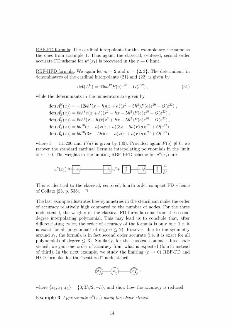
RBF-FD formula: The cardinal interpolants for this example are the same asthe ones from Example 1. Thus again, the classical, centered, second orderaccurate FD scheme for u′′(x1) is recovered in the ε→ 0 limit.

RBF-HFD formula: We again let m = 2 and σ = 2, 3. The determinant indenominators of the cardinal interpolants (21) and (22) is given by

det(AH) = 60bh12F (a)ε20 +O(ε22) , (31)

while the determinants in the numerators are given by

det(AH1 (x)) = −12bh8(x− h)(x+ h)(x2 − 5h2)F (a)ε20 +O(ε22) ,

det(AH2 (x)) = 6bh8x(x+ h)(x2 − hx− 5h2)F (a)ε20 +O(ε22) ,

det(AH3 (x)) = 6bh8(x− h)x(x2 + hx− 5h2)F (a)ε20 +O(ε22) ,

det(AH4 (x)) = bh10(x− h)x(x+ h)(3x+ 5h)F (a)ε20 +O(ε22) ,

det(AH5 (x)) = bh10(3x− 5h)(x− h)x(x+ h)F (a)ε20 +O(ε22) ,

where b = 115200 and F (a) is given by (30). Provided again F (a) 6≡ 0, werecover the standard cardinal Hermite interpolating polynomials in the limitof ε→ 0. The weights in the limiting RBF-HFD scheme for u′′(x1) are

u′′(x1) ≈− 110

− 110 u

′′+ 65

−125

65

u

h2.

This is identical to the classical, centered, fourth order compact FD schemeof Collatz [23, p. 538]. 2

The last example illustrates how symmetries in the stencil can make the orderof accuracy relatively high compared to the number of nodes. For the threenode stencil, the weights in the classical FD formula come from the seconddegree interpolating polynomial. This may lead us to conclude that, afterdifferentiating twice, the order of accuracy of the formula is only one (i.e. itis exact for all polynomials of degree ≤ 2). However, due to the symmetryaround x1, the formula is in fact second order accurate (i.e. it is exact for allpolynomials of degree ≤ 3). Similarly, for the classical compact three nodestencil, we gain one order of accuracy from what is expected (fourth insteadof third). In the next example, we study the limiting (ε → 0) RBF-FD andHFD formulas for the “scattered” node stencil

x3

x1

x2

,

where x1, x2, x3 = 0, 3h/2,−h, and show how the accuracy is reduced.

Example 3 Approximate u′′(x1) using the above stencil.

14

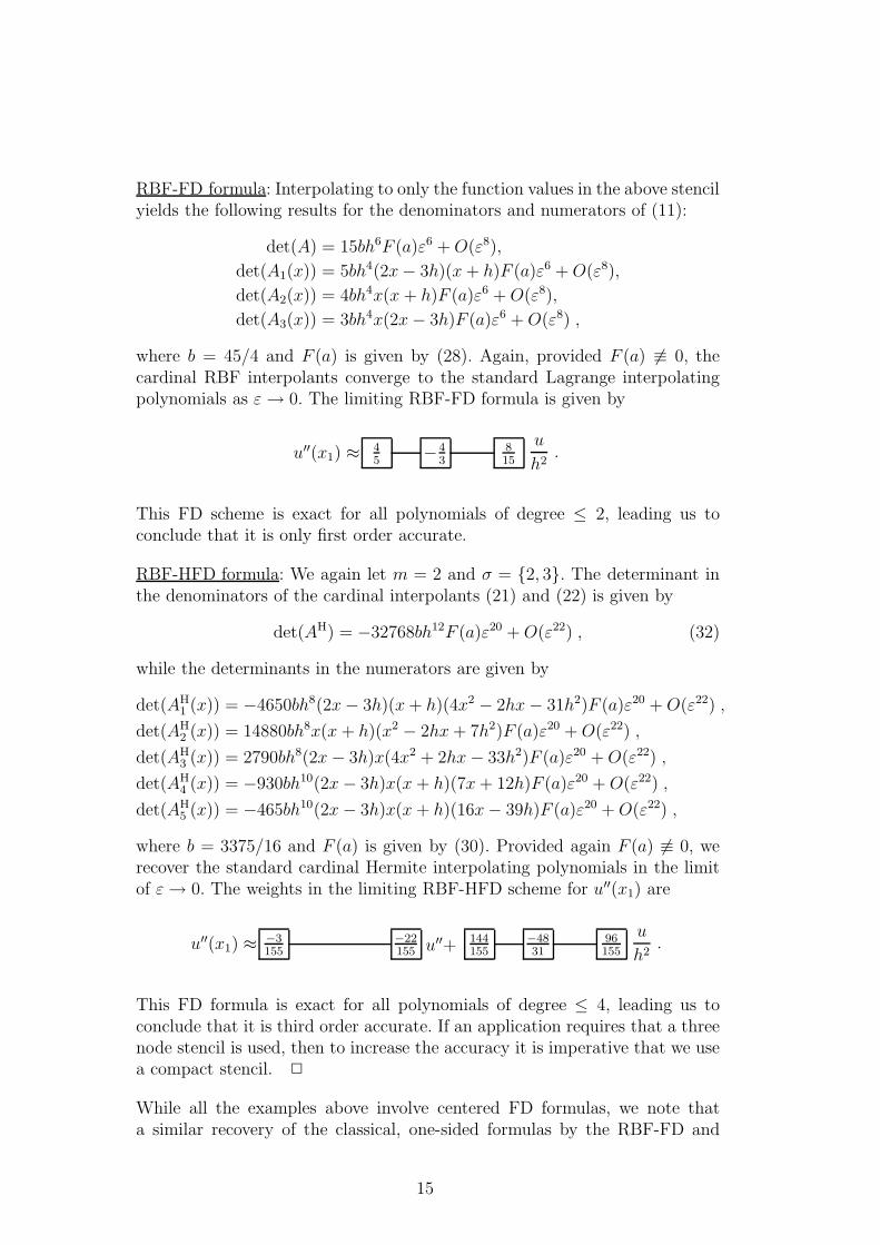
RBF-FD formula: Interpolating to only the function values in the above stencilyields the following results for the denominators and numerators of (11):

det(A) = 15bh6F (a)ε6 +O(ε8),

det(A1(x)) = 5bh4(2x− 3h)(x+ h)F (a)ε6 +O(ε8),

det(A2(x)) = 4bh4x(x+ h)F (a)ε6 +O(ε8),

det(A3(x)) = 3bh4x(2x− 3h)F (a)ε6 +O(ε8) ,

where b = 45/4 and F (a) is given by (28). Again, provided F (a) 6≡ 0, thecardinal RBF interpolants converge to the standard Lagrange interpolatingpolynomials as ε → 0. The limiting RBF-FD formula is given by

u′′(x1) ≈ 45

−43

815

u

h2.

This FD scheme is exact for all polynomials of degree ≤ 2, leading us toconclude that it is only first order accurate.

RBF-HFD formula: We again let m = 2 and σ = 2, 3. The determinant inthe denominators of the cardinal interpolants (21) and (22) is given by

det(AH) = −32768bh12F (a)ε20 +O(ε22) , (32)

while the determinants in the numerators are given by

det(AH1 (x)) = −4650bh8(2x− 3h)(x+ h)(4x2 − 2hx− 31h2)F (a)ε20 +O(ε22) ,

det(AH2 (x)) = 14880bh8x(x+ h)(x2 − 2hx+ 7h2)F (a)ε20 +O(ε22) ,

det(AH3 (x)) = 2790bh8(2x− 3h)x(4x2 + 2hx− 33h2)F (a)ε20 +O(ε22) ,

det(AH4 (x)) = −930bh10(2x− 3h)x(x+ h)(7x+ 12h)F (a)ε20 +O(ε22) ,

det(AH5 (x)) = −465bh10(2x− 3h)x(x+ h)(16x− 39h)F (a)ε20 +O(ε22) ,

where b = 3375/16 and F (a) is given by (30). Provided again F (a) 6≡ 0, werecover the standard cardinal Hermite interpolating polynomials in the limitof ε→ 0. The weights in the limiting RBF-HFD scheme for u′′(x1) are

u′′(x1) ≈ −3155

−22155 u′′+ 144

155−4831

96155

u

h2.

This FD formula is exact for all polynomials of degree ≤ 4, leading us toconclude that it is third order accurate. If an application requires that a threenode stencil is used, then to increase the accuracy it is imperative that we usea compact stencil. 2

While all the examples above involve centered FD formulas, we note thata similar recovery of the classical, one-sided formulas by the RBF-FD and

15

HFD formulas occurs. This is because of the convergence of the regular andHermite RBF interpolants to the standard Lagrange and Hermite polynomialinterpolants, respectively, in the ε → 0 limit.

From the examples above, we see that for each of the RBF-FD formulationswe obtain a set of requirements that the Taylor coefficients of the radial func-tion must satisfy in order for the limiting interpolant to exist. We note thateach of the infinitely smooth functions in Table 1 satisfies the requirementsfrom each example. For larger stencil sizes (i.e. more nodes), the requirementsthat the Taylor coefficients must satisfy become more and more intricate. Forthe standard method in 1-D, the full set of requirements for any number ofnodes was proven in [19] and extended to >1-D in [21] (in both cases, how-ever, a slightly different formulation of the interpolant is considered). The fullset of requirements for convergence in the ε → 0 limit of the Hermite RBFinterpolation method are still unknown. However, experiments suggest theyare similar to the standard case.

The results for the RBF-HFD formulas in the above examples required quiteextensive symbolic manipulation with Mathematica. Extending these resultsto more nodes is, at the present time, intractable. We can, however, nu-merically study the ε → 0 formulas for larger stencils with the Contour-Pade algorithm [33]. Although originally developed for the RBF interpolationproblem, this algorithm can be easily extended for computing the RBF-FDand HFD weights.

4.3 Numerical results using the Contour-Pade algorithm

In the first couple of examples, we further explore the connection betweenlimiting (ε → 0) RBF-HFD schemes and the classical compact FD schemes.We follow this with some results based on scattered node stencils. The resultsof each of the examples in this section are based on the MQ and GA radialfunctions.

Example 4 Approximate u′(x1) and u′′(x1) using the five-node equispacedstencil:

x5

x3

x1

x2

x4 .

The parameters for this example are n = 5, m = 2, and σ = 2, 3. Computa-tions with the Contour-Pade algorithm suggest that the RBF-HFD formulasin the ε → 0 limit converges to the standard, sixth order accurate compact

16

FD formulas [23, p. 538]:

u′(x1) ≈ −13

−13 u′+ −1

36−79 0 7

9136

u

h

and

u′′(x1) ≈ 2−11

2−11 u

′′+ 344

4844

102−44

4844

344

u

h2.

2

Example 5 Approximate ∆u(x1) using the nine-node equispaced stencil:

x8

x4

x7

x5

x1

@@

@

@@@

x3 .

x9

x2

x6

The parameters for this example are n = 9, m = 4, and σ = 2, 3, 4, 5.Computations with the Contour-Pade algorithm suggest that the RBF-HFDformula in the ε → 0 limit converges to the classical, fourth order accuratecompact FD formula [23, p. 542]:

∆u(x1) ≈

−18

−18

−18 ∆u+

−18

14 1 1

4

1 −5

@

@

@@

1u

h2. 2

14 1 1

4

The results for u′′(x1) and ∆u(x1) in the previous two examples illustrate twoimportant observations. First, not including the derivative information resultsin FD formulas that are only fourth and second order accurate, respectively.Second, unlike the compact schemes, these formulas would also not be di-agonally dominant, as we would want from a discrete approximation of theLaplacian. In Section 5, we give evidence that for scattered nodes it is alsomore likely to find a diagonally dominant RBF-FD formula when we make itcompact.

17

m

0 1 2 3 4 5 6 7 8 9 10

n

1 0 0 1 1 1 2 2 2 2 3 32 0 1 1 1 2 2 2 2 3 3 33 1 1 1 2 2 2 2 3 3 3 34 1 1 2 2 2 2 3 3 3 3 35 1 2 2 2 2 3 3 3 3 3 46 2 2 2 2 3 3 3 3 3 4 47 2 2 2 3 3 3 3 3 4 4 48 2 2 3 3 3 3 3 4 4 4 49 2 3 3 3 3 3 4 4 4 4 410 3 3 3 3 3 4 4 4 4 4 411 3 3 3 3 4 4 4 4 4 4 5

Table 2Numerical results for the maximum degree 2-D polynomial the limiting (ε → 0)RBF-HFD formulas for ∆u are exact for using a scattered node stencil. Here n andm are the the number of values of u and ∆u used in the formulas, respectively.

We now focus on the case of a scattered node stencil (cf. Figure 1). As anexperiment, we considered 11 scattered nodes in 2-D and computed the lim-iting (ε → 0) RBF-HFD formulas for approximating ∆u using n values of uand m values of ∆u such that 1 ≤ n ≤ 11 and 0 ≤ m ≤ 10. We then testedthe resulting formulas on all polynomials in the standard basis for polyno-mials of degree ≤ 6. Table 2 displays the maximum degree polynomial theformulas were observed to become exact for. If we let Q equal the maximumdegree polynomial, then the results from the table seem to indicate that when12(Q + 2)(Q + 1) ≤ n + m < 1

2(Q + 3)(Q + 2), the limiting RBF-HFD for-

mula is exact for all polynomials of degree Q. These are the same numberswe would expect if using regular (2-D) polynomial interpolation (with thestandard basis) to generate the FD formulas (assuming these polynomial in-terpolants exist).

5 Application and implementation: elliptic PDEs

In all the numerical experiments that follow, we use the MQ radial functionbecause of its popularity in applications. All of the model problems involve theLaplace linear differential operator, i.e. L = ∆. We note that the d-dimensionalLaplacian and biharmonic operators applied to any radially symmetric func-tion φ(r) are given by

∆φ = (d− 1)1

r

dφ

dr+d2φ

dr2,

∆2φ =d2 − 4d+ 3

r2

[d2φ

dr2− 1

r

dφ

dr

]+ 2(d− 1)

1

r

d3φ

dr3+d4φ

dr4.

18

Also, L1φ(‖x− y‖) = L2φ(‖x− y‖) for the Laplacian.

5.1 Poisson equation on the unit square: uniform discretization

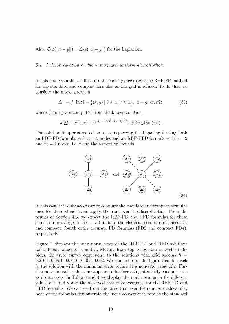
In this first example, we illustrate the convergence rate of the RBF-FD methodfor the standard and compact formulas as the grid is refined. To do this, weconsider the model problem

∆u = f in Ω = (x, y) | 0 ≤ x, y ≤ 1 , u = g on ∂Ω , (33)

where f and g are computed from the known solution

u(x) = u(x, y) = e−(x−1/4)2−(y−1/2)2 cos(2πy) sin(πx) .

The solution is approximated on an equispaced grid of spacing h using bothan RBF-FD formula with n = 5 nodes and an RBF-HFD formula with n = 9and m = 4 nodes, i.e. using the respective stencils

x4

x5

x1

x3 and

x2

x8

x4

x7

x5

x1

@@

@

@@@

x3 .

x9

x2

x6

(34)

In this case, it is only necessary to compute the standard and compact formulasonce for these stencils and apply them all over the discretization. From theresults of Section 4.3, we expect the RBF-FD and HFD formulas for thesestencils to converge in the ε → 0 limit to the classical, second order accurateand compact, fourth order accurate FD formulas (FD2 and compact FD4),respectively.

Figure 2 displays the max norm error of the RBF-FD and HFD solutionsfor different values of ε and h. Moving from top to bottom in each of theplots, the error curves correspond to the solutions with grid spacing h =0.2, 0.1, 0.05, 0.02, 0.01, 0.005, 0.002. We can see from the figure that for eachh, the solution with the minimum error occurs at a non-zero value of ε. Fur-thermore, for each ε the error appears to be decreasing at a fairly constant rateas h decreases. In Table 3 and 4 we display the max norm error for differentvalues of ε and h and the observed rate of convergence for the RBF-FD andHFD formulas. We can see from the table that even for non-zero values of ε,both of the formulas demonstrate the same convergence rate as the standard

19

0 0.5 1 1.5 210

−6

10−5

10−4

10−3

10−2

10−1

100

ε

||err

or|| ∞

RBF-FD, n = 9

0 0.5 1 1.5 210

−12

10−10

10−8

10−6

10−4

10−2

ε

||err

or|| ∞

RBF-HFD, n=9 , m=4

Fig. 2. The error as a function of ε and h for the solution of (33) using the RBF-FDand HFD formulas based on the stencils in (34). Each error curve corresponds to adifferent value of h with varying ε.

FD2 and compact FD4 formulas (i.e. the results for ε = 0). However, for largervalues of ε, the results indicate that h is required to be much smaller beforethe standard rates of convergence are observed.

We conclude this example by noting that for the full range of ε consideredhere, the weights in the RBF-FD and HFD formulas satisfied the diagonaldominance condition

c1 < 0, cj > 0, j = 2, . . . , n, andn∑

j=1

cj = 0 . (35)

Thus, the resulting symmetric, banded linear system for determining the ap-proximate solution (for each ε and h) was guaranteed to be negative definite.

20

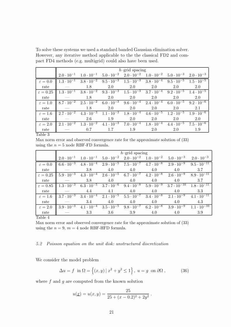
To solve these systems we used a standard banded Gaussian elimination solver.However, any iterative method applicable to the the classical FD2 and com-pact FD4 methods (e.g. multigrid) could also have been used.

h–grid spacing2.0 · 10−1 1.0 · 10−1 5.0 · 10−2 2.0 · 10−2 1.0 · 10−2 5.0 · 10−3 2.0 · 10−3

ε = 0.0 1.3 · 10−1 3.8 · 10−2 9.5 · 10−3 1.5 · 10−3 3.8 · 10−4 9.5 · 10−5 1.5 · 10−5

rate — 1.8 2.0 2.0 2.0 2.0 2.0

ε = 0.25 1.3 · 10−1 3.8 · 10−2 9.3 · 10−3 1.5 · 10−3 3.7 · 10−4 9.2 · 10−5 1.4 · 10−5

rate — 1.8 2.0 2.0 2.0 2.0 2.0

ε = 1.0 8.7 · 10−2 2.5 · 10−2 6.0 · 10−3 9.6 · 10−4 2.4 · 10−4 6.0 · 10−5 9.2 · 10−6

rate — 1.8 2.0 2.0 2.0 2.0 2.1

ε = 1.6 2.7 · 10−2 4.3 · 10−3 1.1 · 10−3 1.8 · 10−4 4.6 · 10−5 1.2 · 10−5 1.9 · 10−6

rate — 2.6 1.9 2.0 2.0 2.0 2.0

ε = 2.0 2.1 · 10−2 1.3 · 10−2 4.1 · 10−3 7.0 · 10−4 1.8 · 10−4 4.4 · 10−5 7.5 · 10−6

rate — 0.7 1.7 1.9 2.0 2.0 1.9Table 3Max norm error and observed convergence rate for the approximate solution of (33)using the n = 5 node RBF-FD formula.

h–grid spacing2.0 · 10−1 1.0 · 10−1 5.0 · 10−2 2.0 · 10−2 1.0 · 10−2 5.0 · 10−3 2.0 · 10−3

ε = 0.0 6.6 · 10−3 4.8 · 10−4 2.9 · 10−5 7.5 · 10−7 4.7 · 10−8 2.9 · 10−9 9.5 · 10−11

rate — 3.8 4.0 4.0 4.0 4.0 3.7

ε = 0.25 5.9 · 10−3 4.3 · 10−4 2.6 · 10−5 6.7 · 10−7 4.2 · 10−8 2.6 · 10−9 8.9 · 10−11

rate — 3.8 4.0 4.0 4.0 4.0 3.7

ε = 0.85 1.3 · 10−3 6.3 · 10−5 3.7 · 10−6 9.4 · 10−8 5.9 · 10−9 3.7 · 10−10 1.8 · 10−11

rate — 4.4 4.1 4.0 4.0 4.0 3.3

ε = 1.6 3.7 · 10−3 3.4 · 10−4 2.1 · 10−5 5.5 · 10−7 3.4 · 10−8 2.1 · 10−9 4.1 · 10−11

rate — 3.4 4.0 4.0 4.0 4.0 4.3

ε = 2.0 3.9 · 10−3 4.1 · 10−4 3.5 · 10−5 9.8 · 10−7 6.2 · 10−8 3.9 · 10−9 1.1 · 10−10

rate — 3.3 3.6 3.9 4.0 4.0 3.9Table 4Max norm error and observed convergence rate for the approximate solution of (33)using the n = 9, m = 4 node RBF-HFD formula.

5.2 Poisson equation on the unit disk: unstructured discretization

We consider the model problem

∆u = f in Ω =(x, y) | x2 + y2 ≤ 1

, u = g on ∂Ω , (36)

where f and g are computed from the known solution

u(x) = u(x, y) =25

25 + (x− 0.2)2 + 2y2.

21

−1 −0.5 0 0.5 1−1

−0.5

0

0.5

1

−1 −0.5 0 0.5 1−1

−0.5

0

0.5

1

(a) (b)

Fig. 3. (a) 200 point unstructured discretization and (b) 201 point structured dis-cretization of the unit disk for the problem in Section 5.2.

The domain is discretized using the N = 200 points shown in Figure 3 (a).The purpose of this example is to compare the RBF-FD and HFD methods onan unstructured grid as ε and the number of nodes in the stencil are varied.

We begin by describing the greedy algorithm used for selecting the nodes foreach of the stencils from the larger unstructured discretization. The essentialfactors used for determining when an acceptable stencil is found are that theweights in the resulting RBF-FD or RBF-HFD formula satisfy the diagonaldominance condition (35) and

1

h2≤ |c1| ≤

2(n− 1)

h2, h = max

i=1,...,n

minj=1,...,n

i6=j

‖xi − xj‖

, (37)

where xi, i = 1, 2, . . . , n are the nodes in the stencil. The first condition guar-antees the linear system for discretizing (36) is negative definite, while thesecond condition is meant to balance the influence of the point the approxi-mation is about. This latter condition would be satisfied by either the standardFD or compact FD formulas on an equispaced grid.

The stencil selection algorithm is as follows: Let N be the number of pointsin the unstructured discretization of the domain Ω and let NI be the numberof points at which to compute all the n-node RBF-FD or HFD formulas. Wedenote each point as xi,1, i = 1, . . . , N , and the nodes that make up the stencilat each point as xi,j, j = 1, . . . , n (note that xi,1 is always part of the stencil).Using the notation from Section 3, we let 0 ≤ m < n be the number ofnodes that contain both function and derivative information. The steps in thealgorithm are as follows:

(1) For each xi,1, i = 1, . . . , NI , determine its η nearest neighbors, where ηis on the order of n.

(2) Compute all possible combinations of choosing n− 1 nodes from these η

22

nearest neighbors and sort them according to their average distance fromnode xi,1. These nodes will be where the function values of the stencil aregiven.

(3) For each set of nodes from the previous step, compute all possible combi-nations of choosingm nodes and again sort them by their average distancefrom xi,1. These nodes will be where the derivative values of the functionare also given.

(4) Looping first over the sorted set of nodes from step 2 followed by thesorted set from step 3, compute the RBF-FD or RBF-HFD formula. Whenthe direct computation becomes unstable for small ε, use the Contour-Pade algorithm [33]. Terminate the nested loops when the weights satisfy(35) and (37).

We make a few comments regarding this algorithm:

• If an acceptable stencil can not be found, one could choose to increaseor decrease n or m. Based on the numerical results from Section 4.3, werecommend trying to keep n+m constant for all the stencils. Additionally,in many cases, the points in the discretization can be chosen freely. Thus, itmay also be possible to move or add some nodes until an acceptable stencilis found.

• In cases where the number of points N in the discretization is large, anefficient search algorithm will be required for determining the points closeto each xi,1; the binning algorithm described by Liu [35, Chap. 15] may beappropriate for this.

• Determining the stencil from the η closest points may not result in the beststencil choice, especially if there are large discrepancies in the discretizationpoints. A possible improvement may be to compute a local Delaunay trian-gulation about the points surrounding xi,1 to determine the points naturalneighbors. This idea is also mentioned in [10].

• If the above algorithm was applied to the equispaced example from theprevious section, then it would immediately select the standard stencils (34)as acceptable. In fact, this default behavior is what guided the algorithmsdevelopment.

Using the above algorithm, we computed RBF-FD formulas with n = 9 nodesfor all the interior points of Figure 3 (a) and for several different values of ε.Similarly we computed two sets of RBF-HFD formulas; one with n = 9, m = 5and the other with n = 10, m = 9. In all cases, acceptable stencils were foundafter very few iterations of the stencil selection algorithm. Figure 4 displaysthe max norm error in the solution to (36) with these formulas as a functionof ε. A point on any of the curves corresponds to the error in the solutionusing the same value of ε in all the stencils. The figure clearly shows that theaccuracy is vastly improved by using the compact stencils. Furthermore, aswe expect, the accuracy can further be improved by increasing the size of the

23

0 0.2 0.4 0.6 0.8 1 1.2 1.4 1.610

−8

10−7

10−6

10−5

10−4

10−3

10−2

ε

||err

or|| ∞

RBF−FD n=9RBF−HFD n=9, m=5RBF−HFD n=10, m=9

FD2 3.0⋅ 10−4

compact FD4 2.8⋅ 10−5

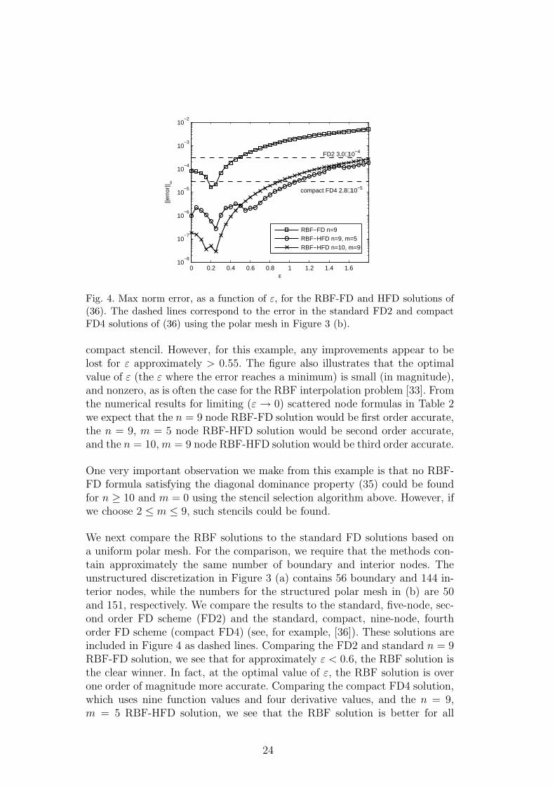
Fig. 4. Max norm error, as a function of ε, for the RBF-FD and HFD solutions of(36). The dashed lines correspond to the error in the standard FD2 and compactFD4 solutions of (36) using the polar mesh in Figure 3 (b).

compact stencil. However, for this example, any improvements appear to belost for ε approximately > 0.55. The figure also illustrates that the optimalvalue of ε (the ε where the error reaches a minimum) is small (in magnitude),and nonzero, as is often the case for the RBF interpolation problem [33]. Fromthe numerical results for limiting (ε → 0) scattered node formulas in Table 2we expect that the n = 9 node RBF-FD solution would be first order accurate,the n = 9, m = 5 node RBF-HFD solution would be second order accurate,and the n = 10,m = 9 node RBF-HFD solution would be third order accurate.

One very important observation we make from this example is that no RBF-FD formula satisfying the diagonal dominance property (35) could be foundfor n ≥ 10 and m = 0 using the stencil selection algorithm above. However, ifwe choose 2 ≤ m ≤ 9, such stencils could be found.

We next compare the RBF solutions to the standard FD solutions based ona uniform polar mesh. For the comparison, we require that the methods con-tain approximately the same number of boundary and interior nodes. Theunstructured discretization in Figure 3 (a) contains 56 boundary and 144 in-terior nodes, while the numbers for the structured polar mesh in (b) are 50and 151, respectively. We compare the results to the standard, five-node, sec-ond order FD scheme (FD2) and the standard, compact, nine-node, fourthorder FD scheme (compact FD4) (see, for example, [36]). These solutions areincluded in Figure 4 as dashed lines. Comparing the FD2 and standard n = 9RBF-FD solution, we see that for approximately ε < 0.6, the RBF solution isthe clear winner. In fact, at the optimal value of ε, the RBF solution is overone order of magnitude more accurate. Comparing the compact FD4 solution,which uses nine function values and four derivative values, and the n = 9,m = 5 RBF-HFD solution, we see that the RBF solution is better for all

24

1 1.2 1.4 1.6 1.8 2

0

0.5

1

1.5

20

100

200

300

400

500

600

ω

RBF−FD, n=9

ε

# of

iter

atio

ns

1 1.2 1.4 1.6 1.8 2

00.5

11.5

20

100

200

300

400

500

600

ω

RBF−HFD, n=9, m=5

ε

# of

iter

atio

ns

(a) (b)

1 1.2 1.4 1.6 1.8 2

00.5

11.5

20

100

200

300

400

500

600

ω

RBF−HFD, n=10, m=9

ε

# of

iter

atio

ns

0 0.5 1 1.5 240

45

50

55

60

65

70

75

ε

min

. # o

f ite

ratio

ns

RBF−FD n=9RBF−HFD n=9, m=5RBF−HFD n=10, m=9

(c) (d)

Fig. 5. (a)–(c) Convergence results of the SOR method for solving the linear systemsassociated with the Poisson model problem as a function of the shape parameterε and SOR parameter ω. (d) Minimum number of iterations required for differentvalues of ε.

values of ε approximately < 1.45. Again, at the optimal ε, the RBF solutionis over one order of magnitude more accurate. Furthermore, the RBF-FD andHFD techniques generalize to more complex domains, while the standard FD2and compact FD4 methods used here are specific to a disk.

We finally make comments on computing the RBF-FD and HFD solutions.The approximate RBF-FD or HFD solution u∗ to (36) at the interior pointsof Ω can be expressed in terms of the linear system

Lcu∗ = (I − Lc)f + b, (38)

where Lc is the matrix containing the RBF-FD or RBF-HFD weights for u, Lc

is the matrix containing the RBF-HFD weights for ∆u (or zeros in the case ofthe RBF-FD formulas), and b contains the contributions from the boundary.Lc is sparse, non-symmetric, and since both the RBF-FD and HFD formulasare required to satisfy (35), it is also diagonally dominant. Many iterativetechniques can be used for solving this system [37, p. 321], we have chosen thethe classical successive over-relaxation (SOR) method. In Figure 5 (a)–(c) we

25

display how the number of iterations necessary for convergence of SOR dependon ε and the relaxation parameter ω for the different RBF-FD methods. Theiterations were terminated when the solution at the ith iteration, u∗

i , satisfied

‖Lcu∗

i −((I−Lc)f +b)‖∞ ≤ 10−9(‖Lc‖∞‖u∗

i ‖∞ + ‖(I − Lc)f + b‖∞). (39)

We can see from the figure that the optimal relaxation parameter dependsquite significantly on the value of ε for the n = 9 RBF-FD solution. However,for both compact solutions, the optimal ω appears to be rather stable withrespect to ε. The choice of ω ≈ 1.6 seems to be good for both compact meth-ods. Figure 5 (d) shows the number of iterations necessary for convergence atthe optimal value of ω for different values of ε. We can see from the figurethat the minimum number of iterations is quite consistent for the compactmethods but jumps around for the non-compact method. There also appearsto be a slight increase in the number of iterations as ε increases. Efficient di-rect solvers based on the FFT may be used for the standard FD2 and compactFD4 polar methods [38] (but only in the specialized case a circular domain).If we had, however, used SOR then the minimum number of iterations wouldbe 162 for FD2 and 328 for compact FD4, which are significantly higher thanthe standard RBF-FD and HFD methods.

5.3 Nonlinear equation: hybrid discretization

As a final example, we consider the nonlinear equation

∆u= e−2xu3 in Ω =(x, y) | x2 + y2 ≥ 0.4 & − 1 ≤ x, y ≤ 1

, (40)

u= g on ∂Ω ,

where g is computed from the known solution

u(x) = u(x, y) = ex tanhy√2.

Note that Ω is square with a circular whole in the middle. To discretize this do-main, we use a hybrid approach that combines an unstructured discretizationnear the hole with an equispaced discretization away from it. Figure 6 illus-trates this discretization. We anticipate that this type of hybrid approach—using scattered nodes only where the geometry is more complex—will be apowerful application of the RBF-FD and HFD methods.

For each node on, and interior to the square enclosed with solid lines in Figure6, we use scattered node RBF-HFD formulas with n = 10 and m = 9 toapproximate the Laplacian. The scattered node stencils are chosen accordingto the stencil selection algorithm of the previous section. For all the other

26

−1 −0.5 0 0.5 1

−1

−0.5

0

0.5

1

Fig. 6. Hybrid discretization for the problem in Section 5.3

interior nodes, we use the same n = 9, m = 4, RBF-HFD formula based onthe second stencil in (34). The scattered node stencils total 252, while theregular stencils total 482.

Let xi = (xi, yi), i = 1, . . . , NI denote all of the interior nodes of the discretiza-tion. Then, using the same notation as (38), we can write the approximationof (40) as

Lcu∗ = D(I − Lc)(u∗)3 + b,

where D is a diagonal matrix with entries Dii = e−2xi, i = 1, . . . , NI andb incorporates the boundary conditions. To solve this nonlinear system ofequations we use Newton-SOR [39, Sec.7.4]. Figure 7 displays the max normerror in the approximate solution as a function of ε. Similar to the previousexample, each point on the curve corresponds to the error using the samevalue of ε in all the RBF-HFD stencils. We can see from the figure that theerror decreases with ε until ε = 0.15, where it reaches a minimum value of1.99 · 10−8.

For the Newton-SOR method, the SOR relaxation parameter was fixed atω = 1.635 for all the Newton iterations and for all values of ε. With thisvalue, the number of SOR sub-iterations required for solving the Jacobiansystem in any one of the Newton iterations varied between 63 and 72. Thesame stopping criterion as (39) was used for the SOR iterations, but with atolerance of 10−10. Finally, we used an initial guess of u = 1 for Newton’smethod. With this value, five Newton iterations were required for the residualto reach a tolerance < 10−12 for all values of ε.

Remark 4 In our experiments, we fixed ε in all of the RBF-FD and HFDformulas and then computed a solution. This may not, however, be the beststrategy. If, for example, the scales associated with each of the RBF-FD orRBF-HFD stencils is significantly different, we may wish normalize ε for each

27

0 0.5 1 1.5 210

−8

10−7

10−6

10−5

10−4

ε

||err

or|| ∞

Fig. 7. Max norm error, as a function of ε, for the n = 10, m = 9 RBF-HFD solutionof (40) using the hybrid discretization shown in Figure 6.

stencil. Two ideas for such a normalization are discussed by Shu et al. [7] andCecil et al. [10].

6 Conclusions

In a similar style to how polynomials are used to generate FD and compactFD stencils for 1-D, we have here shown how RBFs can be used to create anal-ogous formulas also for multidimensional scattered node layouts. We have alsodemonstrated that, when the stencil nodes are arranged accordingly, RBF-FDand HFD formulas in the ε → 0 limit are equivalent to standard FD and com-pact FD formulas. In contrast to many methods, such as finite elements, theRBF-FD or HFD methods do not require the generation of global meshes. Fur-thermore, the number of space dimensions and the geometric complexity of themethods can all be arbitrary without adversely affecting either computationalspeed or algorithmic complexity. Tests with elliptic equations show that accu-racy can be improved dramatically by using RBF-HFD formulas, and that itis imperative to use these formulas to preserve diagonal dominance. The latterproperty permits the use of fast iterative methods for computing the numericalsolution. We believe—but it is yet to be fully explored—that the RBF-HFDapproach will prove successful also for many further classes of PDEs.

Acknowledgements

The authors would like to thank the anonymous referees for their helpfulsuggestions in improving this paper.

28

References

[1] E. J. Kansa, Multiquadrics – a scattered data approximation scheme withapplications to computational fluid-dynamics – II: Solutions to parabolic,hyperbolic and elliptic partial differential equations, Comput. Math. Appl. 19(1990) 147–161.

[2] Y. C. Hon, X. Z. Mao, An efficient numerical scheme for Burgers’ equation,Appl. Math. Comput. 95 (1998) 37–50.

[3] G. E. Fasshauer, Solving partial differential equations with radial basisfunctions: multilevel methods and smoothing, Adv. Comput. Math. 11 (1999)139–159.

[4] E. Larsson, B. Fornberg, A numerical study of some radial basis function basedsolution methods for elliptic PDEs, Comput. Math. Appl. 46 (2003) 891–902.

[5] E. J. Kansa, Y. C. Hon, Circumventing the ill-conditioning problem withmultiquadric radial basis functions: Applications to elliptic partial differentialequations, Comput. Math. Appl. 39 (2000) 123–137.

[6] L. Ling, E. J. Kansa, A least-squares preconditioner for radial basis functionscollocation methods., Adv. Comput. Math. 23 (2005) 31–54.

[7] C. Shu, H. Ding, K. S. Yeo, Local radial basis function-based differentialquadrature method and its application to solve two-dimensional incompressibleNavier-Stokes equations, Comput. Methods Appl. Mech. Engrg. 192 (2003) 941–954.

[8] C. Shu, H. Ding, Numerical comparison of least square-based finite difference(LSFD) and local multiquadric-differential quadrature (LMQDQ) methods,Comput. Math. Appl. submitted (2004).

[9] A. I. Tolstykh, M. V. Lipavskii, D. A. Shirobokov, High-accuracy discretizationmethods for solid mechanics, Arch. Mech. 55 (2003) 531–553.

[10] T. Cecil, J. Qian, S. Osher, Numerical methods for high dimensional Hamilton-Jacobi equations using radial basis functions, J. Comput. Phys. 196 (2004)327–347.

[11] G. Wright, Radial basis function interpolation: Numerical and analyticaldevelopments, Ph.D. thesis, University of Colorado, Boulder (2003).

[12] B. Fornberg, A Practical Guide to Pseudospectral Methods, CambridgeUniversity Press, Cambridge, 1996.

[13] B. Fornberg, Calculation of weights in finite difference formulas, SIAM Rev40 (3) (1998) 685–691.

[14] R. Abgrall, On essentially non-oscillatory schemes on unstructured meshes:analysis and implementation, J. Comput. Phys. 114 (1994) 45–58.

29

[15] W. Schonauer, T. Adolph, How we solve PDEs, J. Comput. Appl. Math. 131(2001) 473–492.

[16] R. J. Y. McLeod, M. L. Baart, Geometry and Interpolation of Curves andSurfaces, Cambridge University Press, Cambridge, 1998.

[17] W. R. Madych, Miscellaneous error bounds for multiquadric and relatedinterpolants, Comput. Math. Appl. 24 (1992) 121–138.

[18] B. Fornberg, N. Flyer, Accuracy of radial basis function interpolation andderivative approximations on 1-D infinite grids, Adv. Comput. Math. 23 (2005)5–20.

[19] T. A. Driscoll, B. Fornberg, Interpolation in the limit of increasingly flat radialbasis functions, Comput. Math. Appl. 43 (2002) 413–422.

[20] B. Fornberg, G. Wright, E. Larsson, Some observations regarding interpolantsin the limit of flat radial basis functions, Comput. Math. Appl. 47 (2004) 37–55.

[21] E. Larsson, B. Fornberg, Theoretical and computational aspects of multivariateinterpolation with increasingly flat radial basis functions, Comput. Math. Appl.49 (2005) 103–130.

[22] R. Schaback, Multivariate interpolation by polynomials and radial basisfunctions, Constr. Approx. 21 (2005) 293–317.

[23] L. Collatz, The Numerical Treatment of Differential Equations, Springer Verlag,Berlin, 1960.

[24] S. K. Lele, Compact finite difference schemes with spectral-like resolution, J.Comput. Phys. 103 (1992) 16–42.

[25] C. A. Micchelli, Interpolation of scattered data: distance matrices andconditionally positive definite functions, Constr. Approx. 2 (1986) 11–22.

[26] R. Schaback, Error estimates and condition numbers for radial basis functioninterpolants, Adv. Comput. Math. 3 (1995) 251–264.

[27] J. Yoon, Spectral approximation orders of radial basis function interpolationon the Sobolev space, SIAM J. Math. Anal. 23 (4) (2001) 946–958.

[28] R. L. Hardy, Multiquadric equations of topograpy and other irregular surfaces,J. Geophy. Res. 76 (1971) 1905–1915.

[29] R. L. Hardy, Theory and applications of the multiquadric-biharmonic method:20 years of discovery, Comput. Math. Appl. 19 (1990) 163–208.

[30] G. E. Fasshauer, Hermite interpolation with radial basis functions on spheres,Adv. Comput. Math. 10 (1999) 81–96.

[31] X. Sun, Scattered Hermite interpolation using radial basis functions, LinearAlgebra Appl. 207 (1994) 135–146.

[32] Z. Wu, Hermite-Birkhoff interpolation of scattered data by radial basisfunctions, Approx. Theory Appl. 8 (2) (1992) 1–10.

30

[33] B. Fornberg, G. Wright, Stable computation of multiquadric interpolants for allvalues of the shape parameter, Comput. Math. Appl. 48 (2004) 853–867.

[34] B. Fornberg, E. Larsson, G. Wright, A new class of oscillatory radial basisfunctions, Comput. Math. Appl.To appear (2005).

[35] G. R. Liu, Mesh Free Methods: moving beyond the finite element method, CRCPress, New York, 2002.

[36] R. C. Mittal, S. Gahlaut, High-order finite-difference schemes to solve Poisson’sequation in polar coordinates, IMA J. Num. Anal. 11 (1991) 261–270.

[37] J. W. Demmel, Numerical Linear Algebra, SIAM, Philadelphia, 1997.

[38] M.-C. Lai, W.-C. Wang, Fast direct solvers for Poisson equation on 2D polarand spherical geometries, Numer. Methods for Partial Differential Equations 18(2002) 56–68.

[39] J. M. Ortega, W. C. Rheinboldt, Iterative Solution of Nonlinear Equations inSeveral Variables, SIAM, Philadelphia, 2000.

31