SCCG Experimental design

"Non-experimental" designs The first issue I will deal with here is that of "non-experimental" studies. This terminology is problematic and would include Diamond's field and natural "experiments" and Hurlbert's mensurative and manipulative experiments. All these studies are situations where the researcher is not able to manipulate the factors of concern and are primarily tools for generating hypotheses to be tested by subsequent studies. If these studies are to be useful they need to be carried out recognising fully their limitations but with adequate care such that the results obtained are the best possible. Loss of idealism does not justify negligence! These studies have weakened inference, rather than no inference. The consequence is that lack of inference limits the extent that the studies can be extrapolated to other cases.

There has been discussion about these alternatives but the literature, as indicated in the examples above, is not consistent in the use of terminology so I have tabulated the alternatives on the basis of key characteristics below. The key issues as I understand them are:

• sampling in space • sampling in time

• the use of before- as well as after- impact sampling • randomisation/interspersion

• replication The table incorporates the key elements of Green's decision tree with other literature to expand the information on "uncontrolled" studies to provide a more complete analysis for managers in local government and other agencies where a lesser design, fully understood, is still superior to prejudice or ignorance. As Hurlbert noted the problem is often the inappropriate use of inferential statistics rather than the design per se and results in “pseudoreplication”. The first distinction, whether the impact has already occurred, in large measure separates Hurlbert's "mensurative" and "manipulative" studies (although there will be cases where the impact has not occurred and manager has no ability to control all the relevant variables) and in these situations I use the term "reference" area rather than "control" (which represents the possibility of randomisation and interspersion only in situations where the impact has not yet occurred).

A classification of "non-experimental" designs?

Has impact already

occurred?

Is when and where known?

Is there a control area? Characteristics of design Terminology

No No Analysis of historical samples to infer impacts over space and time

"Main sequence 5"

"When and where?"

No Single population

Sample over space only "Main sequence 4" "Descriptive studies"

No

Paired populations

Sample over space only

Use of "reference" areas

"Main sequence 4"

"Observational studies"

Yes

Yes

No

Paired populations

Sample over space and time

Use of "reference" areas

"Main sequence 4"

"Analytical studies"

No No Single population

Sample over space and time

"Main sequence 3"

Baseline studies

Prospective studies

No

Single population

Sample over space and time with samples from Before and After impact

"Main sequence 2"

Paired populations


Use of "control" areas

Unreplicated samples

"Main sequence 1"

Control-Impact studies

BACI

No

Yes

Yes Paired populations


Use of "control" areas

Replicated samples

"Main sequence 1"

Control-Impact studies

BACI-M,

BACI-P,

Beyond BACI

"Main sequence #" refers to Green's classification used below

As you might expect, the different tests have different (potential) strengths of inference as indicated below.

"When and where?" - Main sequence 5 The options here are the same as for “inferred impacts” but without knowing when and where the impact first occurred. “In this situation, the strategy must be to determine whether the environmental impact in question existed at times before hypothesised human causes were operating and/or whether it now exists in places unaffected by human activity that might be the cause.”

Spatial-by-temporal framework for sampling designs (Green, 1979) Times before 1 >1 1 1 >1 >1

Times after 1 >1 1 >1 1 >1 Areas

1

Sites per area

1

X XX X X X XX XX X XX XX X XX

1 >1

X X

XX XX

X X X X

X XX X XX

XX X XX X

XX XX XX XX

X X

XX XX

>1 1

X X

XX XX

X X X X

X XX X XX

XX X XX X

XX XX XX XX

X X

XX XX

>1 >1

X X X X

XX XX XX XX

X X X X X X X X

X XX X XX X XX X XX

XX X XX X XX X XX X

XX XX XX XX XX XX XX XX

X X X X

XX XX XX XX

In these surveys historical data, or retesting historical samples, can be used to look for changes (or lack of) to test the hypothesis that some change is causally related to historical events. Where historical samples are not available then you are left with “inferred impacts” (below)

“Inferred impacts” - Main sequence 4 Green notes “too often the environmental biologist is funded to study an impact after its effects have become a problem, and no before impact data can be collected. In this case the impact effects must be demonstrated and described from spatial pattern.” As shown in Green’s table this still allows multiple sites and times to be considered although the “times” samples, all taken after the impact, show natural variability not necessarily variability causal effects due to the impact as you would hope in “controlled” impact studies.



1

Sites per area

1


1 >1

X X

XX XX

X X X X

X XX X XX

XX X XX X

XX XX XX XX

X X

XX XX

>1 1

X X

XX XX

X X X X

X XX X XX

XX X XX X

XX XX XX XX

X X

XX XX

>1 >1

X X X X

XX XX XX XX

X X X X X X X X

X XX X XX X XX X XX

XX X XX X XX X XX X


X X X X

XX XX XX XX

The first distinction is whether a single area is used or, based on some prior factor such as aspect, altitude, catchment condition, prior event, etc, two (or more) blocks are compared. Within an area multiple sites can be assigned depending on the survey design chosen.

Descriptive surveys The descriptive survey estimates a parameter of interest for a single population. The designs used can include:

• simple random sampling • systematic sampling

• cluster sampling • multistage sampling

• multiphase designs • repeated sampling

Standard methods can be used to improve the efficiency of the surveys. These surveys can provide some assessment of a descriptive feature of the population but provide little inference about natural variability or causal relationships.

Observational surveys This is a limited comparative survey between sites but without randomisation or replications to strengthen any inferences from the results.

These are regarded as being essentially similar, if limited in scope, to Analytical surveys in their design and analysis.

Analytical surveys In analytical surveys subpopulations are sampled with appropriate randomisation and replication but the manager does not manipulate the factors of interest. In these cases the first step is to propose explanatory variables and appropriate measurement of response variables. These surveys can be subdivided based on the type of stratification:

• prestratified by the explanatory variables • population surveyed in its entirety and then stratified by explanatory variables

• the explanatory variables can be used as auxiliary variables in ratio or regression methods

The choice between the strategies is usually made by the ease with which the population can be prestratified and the strength of the relationship between the response and explanatory variables. Variables that can be known in advance (altitude, aspect, habitat etc) obviously lend themselves to prestratification but variables that might only be obtained during the survey will, of necessity, be applied later. Prestratification has the advantage of more control over the sample design.

If the surveys have been based on a random design then analysis is similar to designed experiments although the strength of the conclusions is not. Without manipulation strong causal relationships cannot be established. These designs are discussed in more detail in Statistical Methods for Adaptive Management Studies, chapter 3. Methods of analysis of data are discussed in the ANZECC Monitoring Guidelines Chapter 6

Retrospective surveys All the above designs can be grouped as "retrospective surveys", ie where the impact has already occurred and the problem is to explain the sources of the impact. Retrospective studies might use existing data, subject to appropriate quality standards etc., although the primary factor is that the sites are already differentiated by the stress/impact having already occurred. The notion of "retrospective surveys" is from epidemiology where they are defined (with changes in terms) as: "a study in which we initially identify two groups of [sites]:

1. a group that has the [stressor] under study (the cases) and 2. a group that does not have the [stressor] under study (the [reference sites])

We then try to relate their prior and current [environment conditions] to their current [stressed] status."

These designs will have weakened inference but are useful, and even necessary, in a number of circumstances:

• limited funding • long time until results available from a designed experiment

• the need for interim results for management decisions while a controlled study is done

• controlled impacts, especially of natural phenomena, of necessary scale would be unacceptable (flooding, fires, etc)

• historical events where the impacts cannot be controlled (natural invasions, disease outbreaks, etc)

• the need to generate more specific hypotheses prior to initiating large scale/long term studies and/or obtain information on variability in the systems of interest.

These designs are discussed in more detail in Statistical Methods for Adaptive Management Studies, chapter 4.

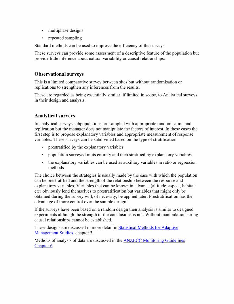
"Baseline or monitoring studies" - Main sequence 3 Green's "main sequence 3” has similar characteristics to "prospective studies" where the impact has not occurred and the sites are monitored, based on the believed characteristics of the stressor of interest. The nature and impact of the stressor is not known specifically and is not under the control of the researcher. The problem is to relate these changes to the environmental characteristics of the sites as the environmental change occurs. Examples might be areas identified for landuse change but where the researcher does not control the rate, specific development characteristics, timing, location of development, etc. If the impacts can be isolated to particular sites then a controlled study becomes possible but if, before hand, you cannot know what will happen, where then this may be the best you can do. The design of these studies should be reviewed as more information becomes available, especially in regard to potential control sites and more specific indication on the factors of concern. These studies may have the advantage over retrospective studies of providing greater inference about causality by sampling over the time impacts and environmental changes occur. See also ANZECC Monitoring Guidelines Chapter 3.2.



1

Sites per area

1


1 >1 X X

XX XX

X X X X

X XX X XX

XX X XX X

XX XX XX XX

X X

XX XX

>1 1 X x X

XX xx XX

X X X X X X

X XX X XX X XX

XX X XX X XX X

XX XX XX XX XX XX

X X X

XX XX XX

>1 >1 X X X X

XX XX XX XX

X X X X X X X X

X XX X XX X XX X XX

XX X XX X XX X XX X


X X X X

XX XX XX XX

“Impact studies - uncontrolled designs” - Main sequence 2 Green’s "impact" surveys refer to situations where the impact has not occurred and we are looking to understand the consequences (potentially positive and/or negative) of the impact (intervention). The designs discussed here occur where an unreplicated event (construction of a dam, major construction, construction of a GPT, etc) has or is about to occur. There may or may not be prior knowledge of conditions from other sampling or there is time to obtain some "before" samples. These result in before and after data but lack adequate controls.

Where the impact has not occurred and where and when are known, but no control is available, surveys are restricted to sampling at different locations at different times, including before and after the impact. Temporal change in spatial pattern can be the criterion for impact effects. Auxiliary parameters might be used, such as precipitation, to relate changes to an independent event; eg amount of suspended solids per mm rainfall in catchment.


Times after 1 >1 1 >1 1 >1

Areas 1

Sites per area

1


1 >1

X X

XX XX

X X X X

X XX X XX

XX X XX X

XX XX XX XX

X X

XX XX

>1 1

X X

XX XX

X X X X

X XX X XX

XX X XX X

XX XX XX XX

X X

XX XX

>1 >1

X X X X

XX XX XX XX

X X X X X X X X

X XX X XX X XX X XX

XX X XX X XX X XX X


X X X X

XX XX XX XX

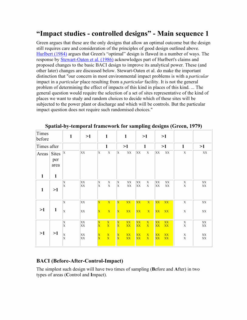
“Impact studies - controlled designs” - Main sequence 1 Green argues that these are the only designs that allow an optimal outcome but the design still requires care and consideration of the principles of good design outlined above. Hurlbert (1984) argues that Green's “optimal” design is flawed in a number of ways. The response by Stewart-Oaten et al. (1986) acknowledges part of Hurlbert's claims and proposed changes to the basic BACI design to improve its analytical power. These (and other later) changes are discussed below. Stewart-Oaten et al. do make the important distinction that "our concern in most environmental impact problems is with a particular impact in a particular place resulting from a particular facility. It is not the general problem of determining the effect of impacts of this kind in places of this kind. ... The general question would require the selection of a set of sites representative of the kind of places we want to study and random choices to decide which of these sites will be subjected to the power plant or discharge and which will be controls. But the particular impact question does not require such randomised choices."



1

Sites per area

1


1 >1

X X

XX XX

X X X X

X XX X XX

XX X XX X

XX XX XX XX

X X

XX XX

>1 1

X X

XX XX

X X X X

X XX X XX

XX X XX X

XX XX XX XX

X X

XX XX

>1 >1

X X X X

XX XX XX XX

X X X X X X X X

X XX X XX X XX X XX

XX X XX X XX X XX X


X X X X

XX XX XX XX

BACI (Before-After-Control-Impact) The simplest such design will have two times of sampling (Before and After) in two types of areas (Control and Impact).

Before After

Control

Impact

The problems with this design are:

1. because impact to the sites was not randomly assigned, any observed difference between control and impacts sites may be related solely to some other factor that differs between the two sites, and

2. if only a single sampling site before and after the impact is used it fails to recognise that natural fluctuations in the characteristic of interest that are unrelated to any impact may occur. An example of the interesting statistical implications of such a design is discussed in Statistics for environmental sampling.

BACI-P(aired) – temporal replication but limited spatial replication BACI-P refers to Before, -After, -Control, -Impact design using Paired observations. In this design, closely matched, but independent, areas are monitored simultaneously at several time periods before the impact occurs, and monitoring continues for several time periods after the impact in both control and impact areas. The difference between control

and impact areas is computed for each sampling time and compared between the before and after periods using a Student t-test or similar technique. If the size of these differences changes after the supposed impact starts, the impact may have been responsible for that change (Stewart-Oaten et al 1986). This design assumes that differences in control and impact areas in the indicator would have remained the same if the impact had not occurred. For many indicators, the main disadvantage of this design is the considerable natural variation in the chosen indicators between randomly selected but very similar areas (Underwood 1991a, 1992, 1993, 1994). It is therefore possible that some disturbance unrelated to the supposed impact may differentially affect either control or impact area. This may result in either the impact being missed or a false conclusion of an impact having occurred, and is most vulnerable to large, local, long-lived disturbances that only affect one of the two areas (Stewart-Oaten et al 1986).

This design is most applicable when there is strong evidence that the indicator is tightly linked to the potential impact and is unlikely to be affected by extraneous, natural factors. The increase in concentration of a highly specific biomarker is one example. Less specific indicators can be used in this design provided there is tight control over impact and control areas, as is the case with streamside or instream life-history assays conducted in aquaria or artificial channels (eg Humphrey et al 1995).

Applying this design to indicators such as populations or community structure is more problematic. Apart from the possibility of missing effects unrelated to the disturbance that might differentially affect one of the areas, this technique assumes there are no trends in the values of the differences across sample dates in either the period before or after the impact. Such trends may be removed by transformation of the data, or the trends could be modeled using regression techniques. Alternatively, the trends may be related to another variable (a ‘nuisance’ variable or covariate) which could then be analysed using analysis of covariance. However, all situations where there are correlations or ‘carry over’ effects from successive sampling times are inferentially weaker than those where successive samples are fully independent. All these techniques have assumptions which must be met. The simple BACI design can be extended by pairing surveys to several selected time points before and after the impact. Both sites sites are measured at the same time points. An analysis of how the difference between the control and impact sites changes over time would reveal if an impact has occurred.

The assumptions that underlie this design are:

1. that the responses over time are independent of each other; where a lack of independence over time tends to produce false positives (Type I errors)

2. the difference in the mean level between control and impact sites is constant over time, and

3. the effect of the impact is to change the arithmetic difference. This may seem irrelevant but where the experimental readings maintain a constant ratio despite an arithmetic difference, such as might occur with concentrations in the water column, effects may be attributed which are not of interest.

Underwood has proposed the Enhanced-BACI design which utilises two temporal scales, ie groups of surveys are undertaken at a longer time scale with (say) three surveys undertaken a week apart randomly located within each group. This design would help distinguish acute and chronic impacts.

Beyond BACI (and Multiple-BACI) The key element to these designs is multiple reference or control sites; there may be one or more impacted sites. The use of multiple control areas allows better characterisation of the natural variation from area to area.

M-BACI – when baseline data can be collected or are available and there are multiple controls M-BACI (Keough & Mapstone 1995) refers to designs where there is more than one control area and several sampling times both before and after the impact. The acronym stands for Before, -After Control, -Impact design with the ‘M’ denoting Multiple control areas; there may be one or more impact areas. Before the supposed impact occurs, two types of areas can be identified: those that will not be subjected to the potential impact and one or more areas that will be subjected to the potential impact. MBACI designs are preferable to the single-control BACIP (section 8.2.5.1/3) and BACI designs (section 8.2.5.1/6); because more control areas are included, the natural variation from area to area is better assessed. Thus if the indicator does change in the impact area relative to the control areas after the impact starts, we can be more confident that this was not due to chance differences between the impact area and the controls. This class of designs is applicable to a wide range of indicators, especially those that vary in space and time. If there is even approximate knowledge of the seasonality of the indicator, and the nature of the impact that needs to be detected, then MBACI designs can be tailored to test for quite specific changes in mean responses. The analytical technique is a form of repeated-measures ANOVA where control and impact areas are re-sampled simultaneously before and after the supposed impact (Faith et al 1995) (Keough & Mapstone 1995). There are some restrictive assumptions attached

to repeated-measures designs, although there are standard methods for accommodating the more routine problems (Winer et al 1991; Green 1993).

Under some circumstances the response variable can take the form of data from paired areas (MBACIP – where the ‘P’ suffix denotes Paired observations). For example using macroinvertebrate community data in rivers, the appropriate response to be measured is change in community structure (represented by an appropriate dissimilarity measure) between upstream and downstream areas on control and impact rivers (eg Faith et al 1995). If an impact occurs, then the change in dissimilarity between upstream and downstream areas will be greater in impacted rivers compared with control rivers. Detecting trends in the responses of indicators can be achieved using regression techniques, although more complex responses will require more intensive sampling through time. As with BACIP designs, short runs of data in the before period are also problematic. For example, if there are natural seasonal changes in the indicator, data should be collected for more than 1 year before the potential impact starts. The precise period needed depends on the lifespan of the organism; long-lived organisms will need longer baselines than short-lived organisms so that assumptions of independence can be satisfied, and any complicated temporal trends modeled accurately. Analysing data for aberrant trends following an impact involves two steps. First, it is important to verify whether there is evidence that such trends might have occurred in the absence of an impact. This is done best by analysing baseline data for trends and analyzing data from control areas for trends in the period after the potential impact has started. The results of these non-impact analyses should be used to assess whether trends in the impact data sets were ‘abnormal’. These comparisons can be done within a complex analysis of covariance framework, or, less formally, by using the trend parameters from analyses at control areas and/or before startup to estimate the confidence limits within which a ‘normally behaving’ system would be expected to lie. If the trend parameters at the impact area after startup lie outside these boundaries, then it would be deemed to be aberrant. It is important to re-emphasise that the amount of baseline and control data will be crucial to the precision of any assessment of whether the impacted area is behaving abnormally. It is also important that there are ample data from the impact area, because the analysis of a trend in the measured variable after startup at the impact area uses not only the last of the pre-impact baseline data but all of the impact data from after startup. To use all baseline data for analyses of ‘trends’ would require that we specified the way in which the variable’s behaviour changed at the time of impact (and after), and then fit the relevant ‘curve’ with an inflexion point at the time of impact to the entire data set. This is likely to be more difficult than breaking the data into segments that represent different conditions (such as pre-impact and post-impact) and analysing the segments separately.

The baseline data collected before the potential impact are also important for planning the timing of sampling after the potential impact starts. Sampling should be arranged differently depending on whether differential seasonal responses are expected. The nature of the impact is also important: the strategy to detect short-term ‘pulse’ impacts differs from that for chronic ‘press’ impacts. These issues are discussed more fully by Keough and Mapstone (1995).

A more serious impediment to using MBACI is the availability of suitable control areas. Optimally, there should be a large number of potentially suitable control areas comparable with the impact area, from which controls can be selected at random. Sometimes, this will not be possible and all potential control areas are used in the study. This may complicate analyses by changing random factors to fixed factors (Keough & Mapstone 1995), and some researchers query whether control and impact areas should ever be regarded as random factors in analyses (eg Hurlbert 1984) because impact areas are rarely chosen at random. Millard and Lettenmaier (1986) argue that the goal of sampling programs is to assess the effect of a particular event on a particular ecosystem rather than to assess the average effect of an event over a number of ecosystems. Whether to regard control and impact areas as random or fixed effects in ANOVA designs for particular situations is an issue that requires further research and debate (Keough & Mapstone 1995).

‘Beyond BACI’ designs These incorporate multiple spatial and temporal scales of sampling and can be viewed as an elaboration of the MBACI group of designs. The designs are useful when the patterns of abundance of the indicator in space or through time are unknown and where identification of appropriate scales of sampling must be identified as part of the program. Underwood (1991a, 1992, 1993, 1994) describes these designs in detail and employed them in a situation where there were scant pre-existing baseline data, where there was a substantial lead-time before the onset of the potential impacts, and where the nature and magnitude of the future potential impacts were unknown. The designs are also well suited to detect changes in the variability of an indicator as well as changes in its mean. Changes in the variability of an indicator may be important if the strategy is to minimise the risk of local extinction or blooms or outbreaks of the indicator in the impact area. Thus, these ‘Beyond BACI’ designs are preferable when the spatial and temporal scales of variation in the indicator are unknown, when little can be specified a priori about the nature of the anticipated impact or when the potential impacts involve a complex mixture of impact patterns (eg simultaneous pulse and press impacts) that need to be identified separately.

As with MBACI designs, data should be collected for a long period before the start of the potential impact, and requires the inclusion of multiple control areas. Because several spatial and temporal scales are being sampled, these programs are likely to be more costly than MBACI designs, and can be complicated to analyse. Moreover, it may be difficult to optimize these designs because a sampling pattern that is efficient for detecting, say, a chronic ‘press’ impact may not very efficient at detecting short-lived ‘pulse’ impacts. Underwood in Underwood & Chapman has illustrated a good "beyond BACI" design.

For additional discussion Statistical Methods for Adaptive Management Studies, Chapter 3, and ANZECC Monitoring Guidelines Chapter 3 are useful.

Documents

SCCG Experimental design