Embed Size (px)
Citation preview
Scenarios for 2050 for a 2-degrees world Using a four regions trade linked IO-model with high sector detail
Choosing Efficient Combinations of Policy Instruments for Low-carbon development and Innovation to Achieve Europe's 2050 climate targets

Page i | Scenarios for 2050 for a 2-degrees world
AUTHOR(S)
Arjan de Koning, Institute of Environmental Sciences (CML) Leiden University
Gjalt Huppes, Institute of Environmental Sciences (CML) Leiden University
Sebastiaan Deetman, Institute of Environmental Sciences (CML) Leiden University
With thanks to:
Dr. Bernd Mayer, GWS - Institute of Economic Structures Research
Project coordination and editing provided by Ecologic Institute.
Manuscript completed in January 2014
Document title Scenarios for 2050 for a 2-degrees world
Work Package WP3: Development of scenarios to 2030 and 2050
Document Type Deliverable 3.1A: Sector detail of the transformation scenarios
Date 31 January 2014
Document Status Final version
ACKNOWLEDGEMENT & DISCLAIMER
The research leading to these results has received funding from the European Union FP7 ENV.2012.6.1-4: Exploiting the full potential of economic instruments to achieve the EU’s key greenhouse gas emissions reductions targets for 2020 and 2050 under the grant agreement n° 308680.
Neither the European Commission nor any person acting on behalf of the Commission is responsible for the use which might be made of the following information. The views expressed in this publication are the sole responsibility of the author and do not necessarily reflect the views of the European Commission.
Reproduction and translation for non-commercial purposes are authorized, provided the source is acknowledged and the publisher is given prior notice and sent a copy.
Scenarios for 2050 for a 2-degrees world | Page ii
Table of Contents
Executive summary 5
1 Introduction 7
2 Emissions profile 2050 consistent with a 2-degrees target 9
3 Method and data 10
4 Scenario 2050: Business As Usual Scenario 12
4.1 Results: emissions 12
4.2 Results: trade volumes 13
5 Scenario 2050: Techno Scenario 14
5.1 Results Techno Scenario 16
5.2 Contributions per sector 16
6 Scenario 2050: Towards a 2-Degrees World scenario 19
6.1 Consumption shifts 19
6.2 Reduced growth 21
6.3 Relating results to the 2-degrees target 23
6.4 Conclusions on 2-Degrees Scenario 24
7 Discussion 25
7.1 Overall reasonableness of outcomes 25
7.2 Changing assumptions 26
8 Interpretation and conclusions 27
8.1 Prediction versus goal oriented scenario analysis 27
8.2 Price and income effects 27
8.3 Comparison with other scenario studies 27
8.4 Conclusions 28
Page iii | Scenarios for 2050 for a 2-degrees world
9 References 29
List of Tables
Table 4-1 Regional exports as percentage of regional GDP 13
Table 5-1 Total electricity supply with respect to 2000 in the 2050 BAU and 2050 TS in percentage 15
Table 5-2 2050 electricity mix (TWh): Techno Scenario 15
Table 5-3 Emissions of CO2 in Gt, compared to different RCP-outcomes 16
Table 6-1 The 8 product groups who’s production is responsible for 20% of CO2 emissions in the Techno scenario if direct emissions from households are excluded from the analysis 19
Table 6-2 GDP growth, growth factor and growth reduction assumption 22
Table 6-3 Emissions of CO2 in the 2-Degrees Scenario with reduced growth and added emission reduction technologies 22
Table 6-4 Emission reduction percentages per region for the 2-degrees target relative to Techno Scenario, according to two principles 23
List of Figures
Figure 3-1 GDP, Population and GDP for 2000; 2050 BAU; and Techno Scenario 11
Figure 4-1 Territorial CO2 emissions in: 2000; BAU 2050; and Techno Scenario 2050 13
Figure 5-1 Global aggregate sector emissions of CO2, CH4 and N2O 17
Figure 5-2 Contribution to CO2 emissions in Manufacturing and Transport services sectors 18
Figure 6-1 Effect of shifting expenditure from carbon intensive products to low carbon intensive products on the 2050 Techno scenario. The red background represents the 2050 Techno Scenario. The grey foreground represents the expenditure shifted scenario. The red that ‘peeps’ out under the grey graph is the CO2 emission reduction accomplished by the expenditure shift. 21
Figure 6-2 Emission reductions for a 2-degrees target, two principles, see green and blue 23
Scenarios for 2050 for a 2-degrees world | Page iv
LIST OF ABBREVIATIONS
2DS Towards-2-degrees scenario
AR5 Fifth assessment report
BAU Business as usual
BRICs Brazil, Russia, India, China
BX BRIC countries plus Turkey, Indonesia and South Africa
CCS Carbon capture and storage
EU European Union
GDP Gross domestic production
HI High Income countries
IEA International Energy Agency
IPCC Intergovernmental Panel on Climate Change
nec Not elsewhere classified
OECD The Organisation for Economic Co-operation and Development
RCP2.6 Representative concentration pathway leading to a 2.6 W/m2 radiative forcing which has a high probability to limit global mean temperature increase to 2°C.
RoW Rest of World
TS Techno scenario
WP Work package
Page 5 | Scenarios for 2050 for a 2-degrees world
Executive summary
A trade linked global input-output table with environmental extensions has been constructed for the year 2000. The data come from EXIOBASE, which has a 44 country/region detail covering the whole world. These countries have been aggregated into four global regions: the EU; other developed countries; fast developing countries; and a Rest of the World. These regions are treated as internally homogeneous. The sector detail is around 129 sectors. All sectors are trade-linked globally. A global final demand vector reflecting expected economic growth per region quantifies all sectors, resulting in the CO2 emissions of each sector in each region. These can be added into regional and global emissions and into emissions of regional consumption, reckoning with upstream emissions in other regions.
On this basis three scenarios have been constructed for the year 2050, in a transparent stepwise procedure, which includes assumptions on development towards 2050. These assumptions are specified in detail and can be varied easily. This scenario machine, including the basic data, is open for use by others, downloadable without restrictions. The three scenarios are first a Business-as-Usual (BAU) scenario, introducing general growth assumptions using OECD foresights; a Techno-Scenario (TS), adding a number of climate technologies and shifts in energy production to BAU; and the Towards-2-Degrees Scenario (2DS), with a demand shift added to TS, intended to reach an emission level consistent temperature rise of not more than two degrees (in line with RCP2.6 in AR5).
The results of the three scenarios are roughly in line with most other scenario models. The high growth in the fast developing countries and the substantial growth in the Rest of the World reduce the share of rich countries in global climate emissions to a minor fraction. The two degrees target seems difficult to reach with advanced climate saving technologies alone. Even substantial shifts in consumption styles are not enough. Reducing assumed growth below OECD foresight is one option. But that would imply that the fast developing countries, the main emitters by then, would grow less fast. This would imply an even larger difference in income per head remaining, relative to the now already rich countries which is unrealistic. Global trade does not increase as a percentage of global income. However, the embodied emissions in imports increase to well over 30% for the EU. These embodied emissions reduce the regional effects of changes in consumption structure taken by one region.
The overall outlook in this scenario study is not optimistic. Emissions from steel and cement production and air and sea transport become dominant. They are difficult to reduce. Using biofuels in air and sea transport does not work, as biomass is used for electricity production already with 80% CCS, as holds for all remaining fossils as well. One option might be

Scenarios for 2050 for a 2-degrees world | Page 6
hydrogen, produced by near zero emission sources. It seems that a more pervasive pressure towards emission reduction is required, also influencing the basic fabric of society in terms of types and volumes of energy use, materials use and transport. Reducing envisaged growth levels, hence reducing global GDP per head, might be one final contribution needed for moving to the two-degrees target, not on political agendas now. Other sets of assumptions may easily be applied to the model by others, as all basic data on the regions are freely available.
Page 7 | Scenarios for 2050 for a 2-degrees world
1 Introduction
Different kinds of modelling of economic activities for assessing climate change all have their strength and weaknesses. They range from energy optimization models to partial equilibrium models and to general equilibrium models, and may include relations based on a number of econometrically established trends. Applications of these models can be found in MNP (2006), IEA (2013) and Hourcade et al (2006). Background assumptions are required to specify exogenous developments. Such assumptions may also define scenarios. Assumptions and endogenous relations can vary widely, leading to diverging outcomes. Interpreting such outcomes requires insight in assumptions and relations. More complex models, having larger numbers of endogenous relations, are also more complex in their interpretation. Especially when covering longer time horizons, of decades, predictions are not really possible. For that time horizon models give insight in a number of mechanisms relative to each other and relative to varying assumptions.
In the scenario model developed in this study, we exclude all endogenous empirical relations. The situation depicted in 2050 is fully based on assumptions; there are no endogenous dynamic relations. The ultimate core assumption is based on the desired output: remaining within the 2-degrees maximum window of opportunity, as specified in the RCP2.6 climate scenario (Vuuren et al., 2011). All other assumptions align with moderate views on population development, economic growth, energy technology development and emission reducing measures like Carbon Capture and Storage. If all our input assumptions don’t lead to the desired emission output, we finally have to turn on the knobs on final consumption, shifting consumption patterns, also between different final use energy expenditure types. We fill in these exogenous assumptions in EXIOBASE, a highly detailed global IO database with environmental extensions (Tukker et al., 2013). Then we get a hint of how the world might look like in 2050. Starting point is the world as described in 2000 in EXIOBASE, stepwise transformed into possible worlds in 2050. The first step is to introduce trends in energy efficiency improvement and expectations on economic growth, taken from the OECD (2012a). This creates a Business-As-Usual scenario (BAU) assuming no influence of specific climate policies. Next, in step 2, specific emission reducing technologies are introduced, including a shift to electricity in broad domains in industry and private households; a shift in electricity mix towards renewables and less use of coal; and extensive use of CCS. We call this the Techno Scenario (TS). Finally, in step 3, final demand structure is adapted for further emission reduction, the Towards-2-Degrees Scenario (2DS). Measures to be taken seem so extreme however that we stopped short of the 2-degrees target.
Excluding all causal mechanisms of course leaves out all empirical dynamics. This is a blessing in disguise as this allows for a straightforward interpretation: it is only the assumptions
Scenarios for 2050 for a 2-degrees world | Page 8
determining results. However, the IO accounting framework has one reality advantage. It systematically links all global activities, connected through trade flows. All detailed sectoral inputs have been produced by other sectors somewhere in some country, and all final consumption in each country is linked to production chains somewhere in the world. Global trade is fully detailed. Local actions can thus be analysed as to their global consequences. The result gives a hint of what a 2-degrees future might look like. Overall consistency is the key characteristic. Though no explicit behavioural feed-back mechanisms are endogenised, these outcomes do include effects otherwise difficult to grasp. An example is the economic growth effects of energy efficiency improvement. Does it reduce our energy consumption or are we set for a new age of Jevons paradoxes? Predictive modelling over half a century could hardly give an answer to this question. Our results show that neither of these will be the case. Our reasonable assumptions squeeze the scenario within reasonable boundaries. This allows for a more focused discussion, not on what might happen, widely diverging, but on the assumptions that keep the outcomes in the domain they are in. We will not yet go for a sensitivity analysis on assumptions, though definitely that is the role the static IO model should play in due time. In this paper the framework for such an analysis on assumptions has been developed.
We first specify the 2-degrees target in terms of an emission profile for 2050. Then the stepwise methodology is specified. Next, we specify the main assumptions for the first two scenarios (BAU and TS), giving an outcome in terms of climate changing emissions which is not yet in line with the two degrees target. In the third step, there are two knobs to turn to arrive at max 2-degrees. First we look at shifting consumption from high emission intensity products to low emission intensity products, reckoning with the full also inter-regional supply chain. This is different from other options for improving climate performance, like shifting to production in the most efficient regions, as has been studied by Strømman et al. (2009). Because a shift in final demand is not enough to reach the 2-degrees target, finally strong assumptions on reduced economic growth have been introduced. This reduction goes beyond what might be feasibly achieved voluntarily on reducing growth, as by increasing leisure time and so producing and consuming less. The growth reduction also leads to increased inequality. All such assumptions, and other ones, may be applied with relative ease in the scenario framework as developed, which then may function as a scenario tool.
Page 9 | Scenarios for 2050 for a 2-degrees world
2 Emissions profile 2050 consistent with a 2-degrees target
The 2-degrees target does not refer to one specific emission level in 2050. With an earlier start of emission reductions, later reductions can be more modest. Conversely, a not so early start would require more extreme reductions later. What would be a realistic assumption on the speed of effective implementation of stringent climate policy? From the surveys of 2-degrees scenarios (see Vliet et al., 2009) we choose a middle option with higher emission reductions after 2050. This still seems quite optimistic, given the undisturbed rising trend in CO2 concentrations up till now. The 2050 target in terms of GHG emissions are set at a total world emission of 18 Gt CO2 eq per year. This corresponds to an emission pathway with a radiative forcing in 2100 of 2.6 W/m2 (RCP2.6, 450 ppm CO2-eq) with an overshoot before 2050 allowed. We assume that the 18 Gt CO2 equivalent contains 70% CO2, giving a separate CO2 target of 12.6 Gt worldwide in 2050, the remainder being the total volume of all non- CO2 emissions in CO2 equivalent terms.
We have chosen to focus the analysis on CO2 only although CH4 and N2O emissions – the main non-CO2 emissions – are available in our data set as well. We did so because policies for emissions of methane and N2O are more difficult to develop and implement than for CO2, as direct emission measurement mostly is not feasible. Nor is indirect measurement as is the case with CO2 emissions measured through the carbon content of fuels. Methane from paddy rice production is an example where measurement seems quite impossible. N2O emissions - mostly in biomass production - also cannot usually be measured at source. They will tend to rise due to more intense land use because of rising food and fodder production and rising biomass-for-energy production.
Scenarios for 2050 for a 2-degrees world | Page 10
3 Method and data
The EXIOBASE supply-and-use tables (SUTs) form the basis for specifying the scenarios. This world model distinguishes 44 trade-linked countries/regions, including the EU27 as a group, with around 129 sectors per country (in practice not every sector exists in each country). In EXIOBASE, the national supply-and-use tables have been trade-linked. This means that all sectors in each country/region are consistently linked to the supplying and using sectors in all other countries/regions. As national supply-and-use data and trade data all have their flaws, consistency is approached by adapting flows. The GRAS method used (Junius & Oosterhaven, 2003), chooses the smallest level of adaptation so as to reach (near) consistency. There is not a separate consumption activity in the SUTs, as for example had been added in the EIPRO-study (Tukker et al., 2006). The most important household emissions as in household natural gas use and combustion emissions of private cars have however been added in the framework. The structure of final consumption in 2050 converges to the European consumption structure in all regions, with the adaptations as added in the scenario assumptions.
The EXIOBASE data on 2000 are some of the most detailed and thoroughly available now. The IO scenario framework may later be updated with newer data, as coming up in another EU FP7 project, CREEA (delivery date spring 2014). The EXIOBASE emission data cover the major greenhouse gases CO2, CH4, and N2O. Data on other emissions, like particulate matter, NOx and SOx, are available, for example to specify co-benefits of climate policies, but have not been used in this project.
As no behavioural mechanisms like market mechanisms are included which would change relative prices, the scenarios are in constant prices (year 2000) for all products. The conversion between monetary flows and physical flows therefore is straightforward. In the scenarios, new technologies are added in monetary terms, directly corresponding with their underlying physical composition and emission factors, at the given prices. These underlying physical specifications are not part of the SUT framework but can be found in the technical Annex A. There is no hybrid analysis in the sense of combining monetary and physical flow units.
All assumptions on economic and technical development relate to four different world regions: The EU; other High Income Countries, like the US and Japan; Newly Developing Countries, like the BRICs; and a Rest of the World, including most African and Middle Eastern countries. The OECD prospects (OECD 2012a and 2012b) for economic growth have been distributed over these four regions, equal for all countries in each region. Outcomes in terms
Page 11 | Scenarios for 2050 for a 2-degrees world
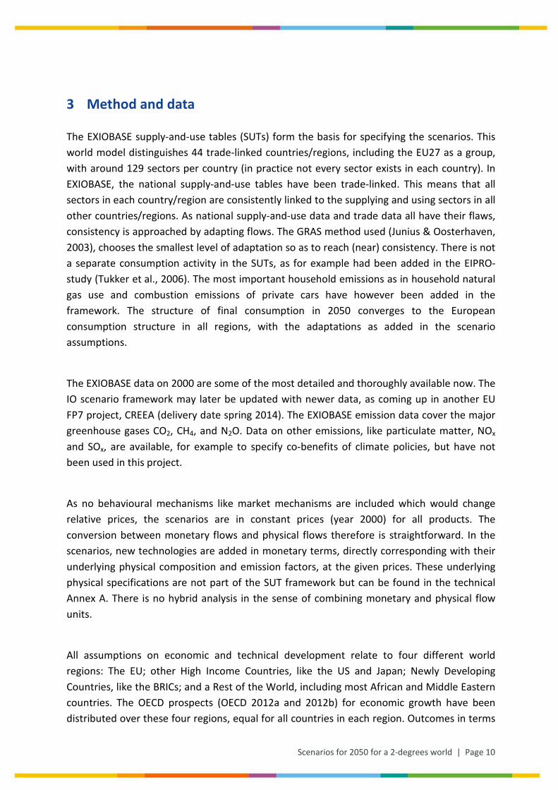
of GDP 2050 differ sharply, as can be seen from Figure 3-1. The EU will grow by a bit over a factor 2 from 2000 to 2050; Other Developed Countries slightly less; Newly Developing Countries by a factor close to 10; and the Rest of the World by a factor 4.5. Technology shifts and demand shifts together are to reduce the otherwise rapidly rising climate emissions to the desired level for 2-degrees. In the active scenarios, growth data have not been corrected for the real costs of climate policy, giving a slight overestimate in real growth. This overestimate may be seen as corrected when reducing demand in the Towards-2-Degrees Scenario. See Figure 3-1 for a survey of the economic data, including the - quite similar - data for the Techno Scenario.
Figure 3-1 GDP, Population and GDP for 2000; 2050 BAU; and Techno Scenario1
1 All results data and figures are available in a downloadable excel file. For more information see Annex C.
0
5000
10000
15000
20000
25000
30000
35000
40000
EU HI BX RoW
billio
n E
uro
GDP
0
500
1000
1500
2000
2500
3000
3500
4000
4500
EU HI BX RoW
milli
on
Population
0
10000
20000
30000
40000
50000
60000
EU HI BX RoW
Eur
o
GDP per capita
20002050, BAU2050, Techno
Scenarios for 2050 for a 2-degrees world | Page 12
4 Scenario 2050: Business As Usual Scenario
Mechanisms for population growth, general efficiency improvement and productivity growth together lead to a more or less autonomous development, already influenced by policies and other considerations. These general developments have been implemented in the EXIOBASE SUT in the following ways. The trends in general efficiency improvement of the last decade have been extrapolated, looking in detail into the developments of the 30 most energy consuming sectors at NACE rev1.1, Level 2, as derived from the WIOD database (Timmer, 2012). These trends are not substantial for developed countries, at roughly 1% over the scenario period, and are somewhat higher for high growth developing countries. These generic efficiency increases next are added, and the full system is scaled so as to reflect OECD expectations on overall economic growth. The shift in developed countries towards the secondary and tertiary sectors partly is due to shifting abroad of material production to emerging countries. At a global level such a shift is not possible and is not reflected in our total data. Likewise visions of re-industrializing Europe are also not explicitly included in our scenarios.
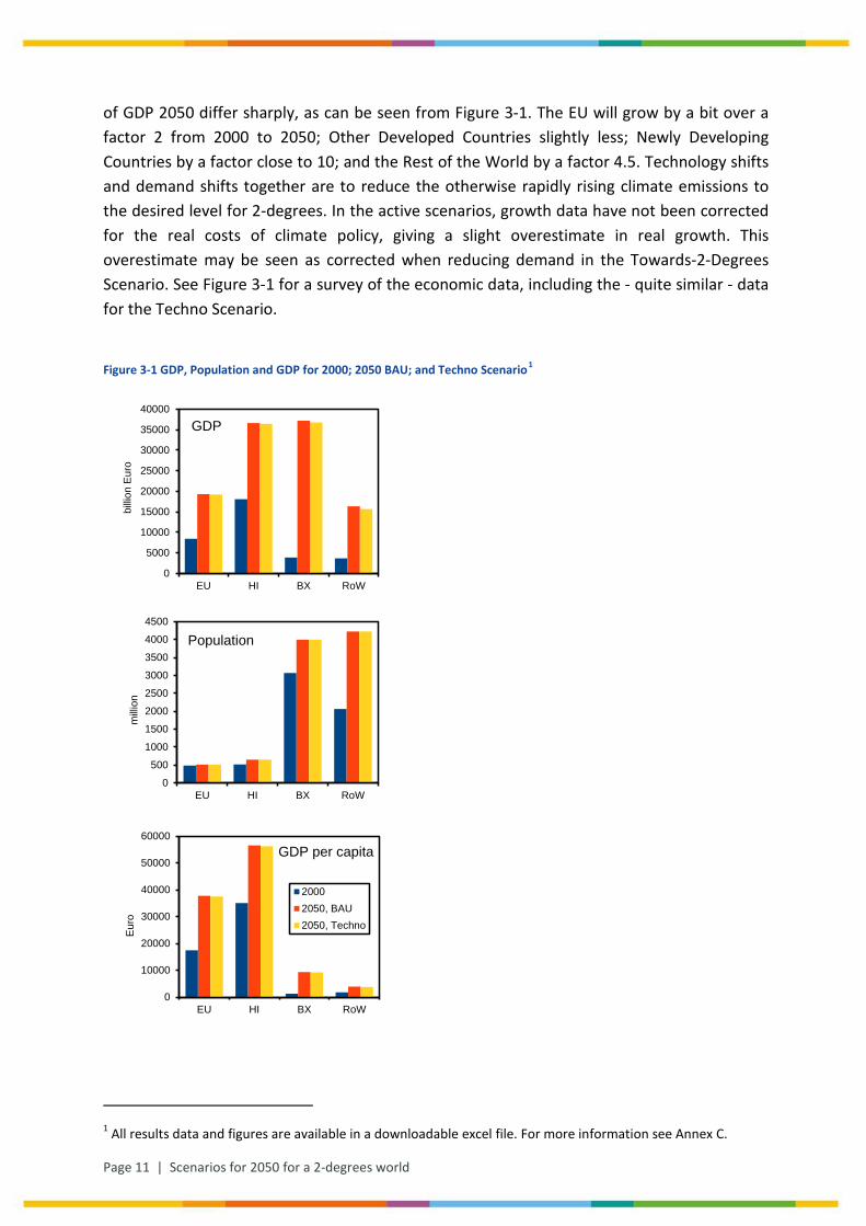
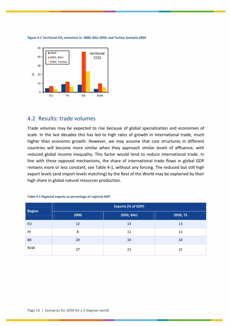
4.1 Results: emissions The emission in the BAU scenario amount to 94 Gt CO2 eq/yr. This is a manifold of 18 Gt CO2 eq/yr in 2050, corresponding the 2-degrees target. Because the business-as-usual scenario is used as a reference on which GHG emission mitigation assumptions are superimposed, the estimated GHG emission in the BAU scenario are a key starting point. The assumption on higher BAU GHG emissions in 2050 implies that reaching a 2 degrees target seems more difficult. Our estimate of 75 Gt CO2/yr emissions in 2050 are on the high end compared to the BAU scenarios by the OECD (2012a). This study uses the growth and population forecasts as specified in the OECD Environmental Outlook. The OPECD model used in the OECD report results in a CO2 emission of 60 Gt CO2/yr, while our results are higher, in the range of 75 Gt CO2/yr. However, the IPCC survey of BAU outcomes on GHG emissions range from under 40 to over 100 Gt CO2/yr in 2050 (Moss et al., 2010, Meinshausen et al., 2011), so our outcomes are in the middle range. Our starting point of 75 Gt CO2/yr aligns with the IPCC RCP8.5 scenario, as reported in the RCP database (Riahi et al., 2007). Even the combined emissions of CO2, CH4 and N2O of 94 Gt CO2 eq/yr in 2050 is similar to the IPCC RCP8.5 scenario. But the distribution of the emissions over the regions is quite different (see also Figure 4-1). Especially fewer emissions will come from the RoW compared to the IPCC RCP8.5 scenario. Because our scenario and the IPCC RPC8.5 scenario are both based on a business as usual assumptions, the correspondence between their results therefore gives some confidence in our modelling approach.
Page 13 | Scenarios for 2050 for a 2-degrees world
Figure 4-1 Territorial CO2 emissions in: 2000; BAU 2050; and Techno Scenario 2050
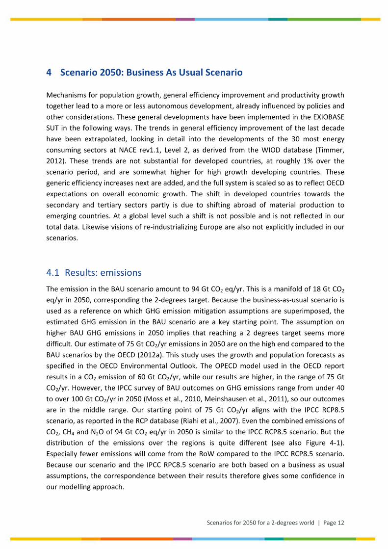
4.2 Results: trade volumes Trade volumes may be expected to rise because of global specialization and economies of scale. In the last decades this has led to high rates of growth in international trade, much higher than economic growth. However, we may assume that cost structures in different countries will become more similar when they approach similar levels of affluence, with reduced global income inequality. This factor would tend to reduce international trade. In line with these opposed mechanisms, the share of international trade flows in global GDP remains more or less constant, see Table 4-1, without any forcing. The reduced but still high export levels (and import levels matching) by the Rest of the World may be explained by their high share in global natural resources production.
Table 4-1 Regional exports as percentage of regional GDP
Region Exports (% of GDP)
2000 2050, BAU 2050, TS
EU 12 13 13
HI 8 11 11
BX 20 10 10
RoW 27 21 21
0
10
20
30
40
50
EU HI BX RoW
Gt
territorial CO2
20002050, BAU2050, Techno
Scenarios for 2050 for a 2-degrees world | Page 14
5 Scenario 2050: Techno Scenario
The Techno Scenario introduces emission reducing technologies to a substantial degree, including a substantial shift to electricity production to allow for substantial CCS when using fossil fuels and to accommodate a substantial share of wind and solar. So electricity production increases substantially, not only for economic growth but also for the electrification of society, in transport and households. Technologies change substantially. The new coal and gas fired power stations are all equipped with CCS reducing CO2 emissions with 80%; all biomass for energy is used for electricity (and heat) production, equipped with CCS. For that level of CCS, probably large scale transport systems are required to bring the CO2 from major sources of incineration to large saline aquifers. Such details have been accounted for based on average additional material and energy requirements, based on (NETL, 2010).
Shifts in primary energy for electricity production are substantial in our scenario (based on Jakeman and Fisher, 2010), with large increases in the share of biomass, a substantial increase in the share of other renewables, and a relatively constant share of nuclear, see Table 5-2. The electricity supply mix could have been chosen such that renewables would have a (much) higher share. However, based on rates of penetration of new renewable technologies (Kramer & Haigh, 2009), the long lifetime of coal power plants that are being built today and the shale gas revolution, it seems not unreasonable that even in 2050 fossil fuel based electricity generation still plays a substantial role. Even though the shares of some electricity generation stay the same (e.g. nuclear) it implies tremendous absolute growth, as electricity use expands so much, see Table 5-1. In this technology oriented step, energy using industries adapt their source of energy in line with the overall assumptions on shifts in primary energy input.
There are similar shifts in final consumption, where cars mainly use electricity, replacing fossil and biomass fuel, the biomass being applied in larger installations with high level CCS. There are some exceptions like iron and steel production, cement production, small scale manufacturing and ocean and air transport, where fossils remain dominant without capture of the emitted CO2. Specific emission reduction strategies for CH4 and N2O have been proposed (Lucas et al., 2007) but not implemented in the scenarios. The focus has been on CO2 emission reduction scenarios.
Page 15 | Scenarios for 2050 for a 2-degrees world
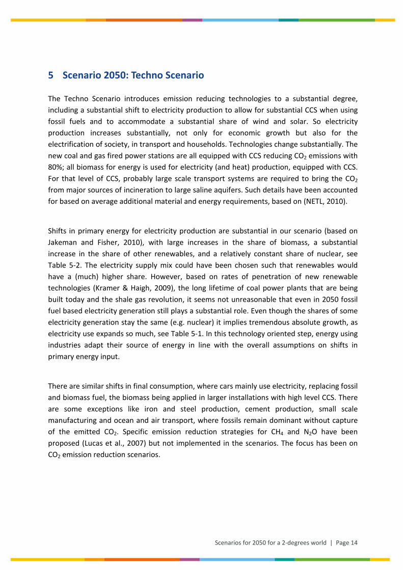
Table 5-1 Total electricity supply with respect to 2000 in the 2050 BAU and 2050 TS in percentage
Region 2000
(%) 2050, BAU
(%)
2050, TS
(%)
EU 100 177 123
HI 100 162 152
BX 100 742 642
RoW 100 347 306
Other final demand categories - that is their shares - have been kept constant in this technology oriented scenario. Food and beverages do not change, let alone that diet assumptions have been introduced. That is part of step 3, to get closer to the 2-degrees target. See Annex A for a full survey and quantification of the technologies introduced in this scenario step.
The technologies are added in the SUT-framework in monetary terms, corresponding with underlying physical composition and emission factors, all at constant prices. The technologies specified take the place of a number of technologies as specified in the BAU scenario. They are added to these BAU developments. These general technology developments are quite substantial in their emission reductions and cover around 15% of emissions in all sectors. Cement production reduces CO2 emissions by 3%; iron and steel uses 6% less coal and about 50% less natural gas.
Table 5-2 2050 electricity mix (TWh): Techno Scenario
Production source EU
(%)
HI
(%)
BX
(%)
RoW
(%)
Coal 11.2 31.7 16.8 15.8
Natural gas 25.3 16.1 19.4 19.8
Nuclear 34.0 26.5 13.3 15.5
Hydro 10.9 6.2 34.4 32.8
Wind 6.6 7.6 4.1 4.0
Solar, biomass; waste 12.0 12.0 12.0 12.0
Total 100.0 100.0 100.0 100.0
Scenarios for 2050 for a 2-degrees world | Page 16
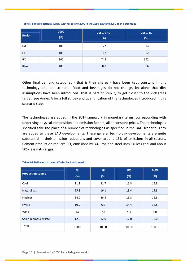
5.1 Results Techno Scenario The results for the Techno Scenario are in Table 5-3 and in Figure 4-1. They show that the heavy introduction of emission reducing measures, including 80% CCS on the remaining coal and gas use and also 80% on bioenergy, is enough to reduce the emissions of the developed countries (EU and HI) by nearly 30% relative to 2000. However the sum of such measures is not enough to reduce emissions in the two developing world regions (BX and RoW) below the 2000 level. For the world as a whole CO2 emissions increase from 26 to 39 Gt, more than three times the 2-degrees target of 12.6 Gt in 2050. Special attention is due on the role of the BX region (including China, India, Indonesia and Brazil), taking more than half of all emissions. The emission reduction measures in the Techno Scenario reduce CO2 emissions by about 50% compared to BAU in each region. Because the emission estimates in BAU 2050 for the BX countries are high as compared to IPCC RCP scenarios the contribution of BX in 2050 under the Techno Scenario is high as well. The total emissions in our Techno scenario in 2050 are very much similar to the IPCC RCP4.5 emission scenario (Clarke et al., 2007) for 2050 but the distribution between the BX and the RoW regions is quite different. However without knowing what emission reduction measures have been implemented in the RCP4.5 scenario compared to our Techno Scenario it is not really possible to compare the two scenarios in content.
Table 5-3 Emissions of CO2 in Gt, compared to different RCP-outcomes
Region Actual Year 2000 BAU Scenario
2050 Techno Scenario
2050 IPCC RCP8.5
2050 IPCC RCP4.5
2050
EU 4.6 7.0 3.6 4.8 3.1
HI 9.1 12.0 6.3 15.9 6.3
BX 8.6 45.8 23.7 34.6 18.0
RoW 3.9 10.0 5.7 17.9 13.1
Total 26.2 74.8 39.3 73.2 40.5
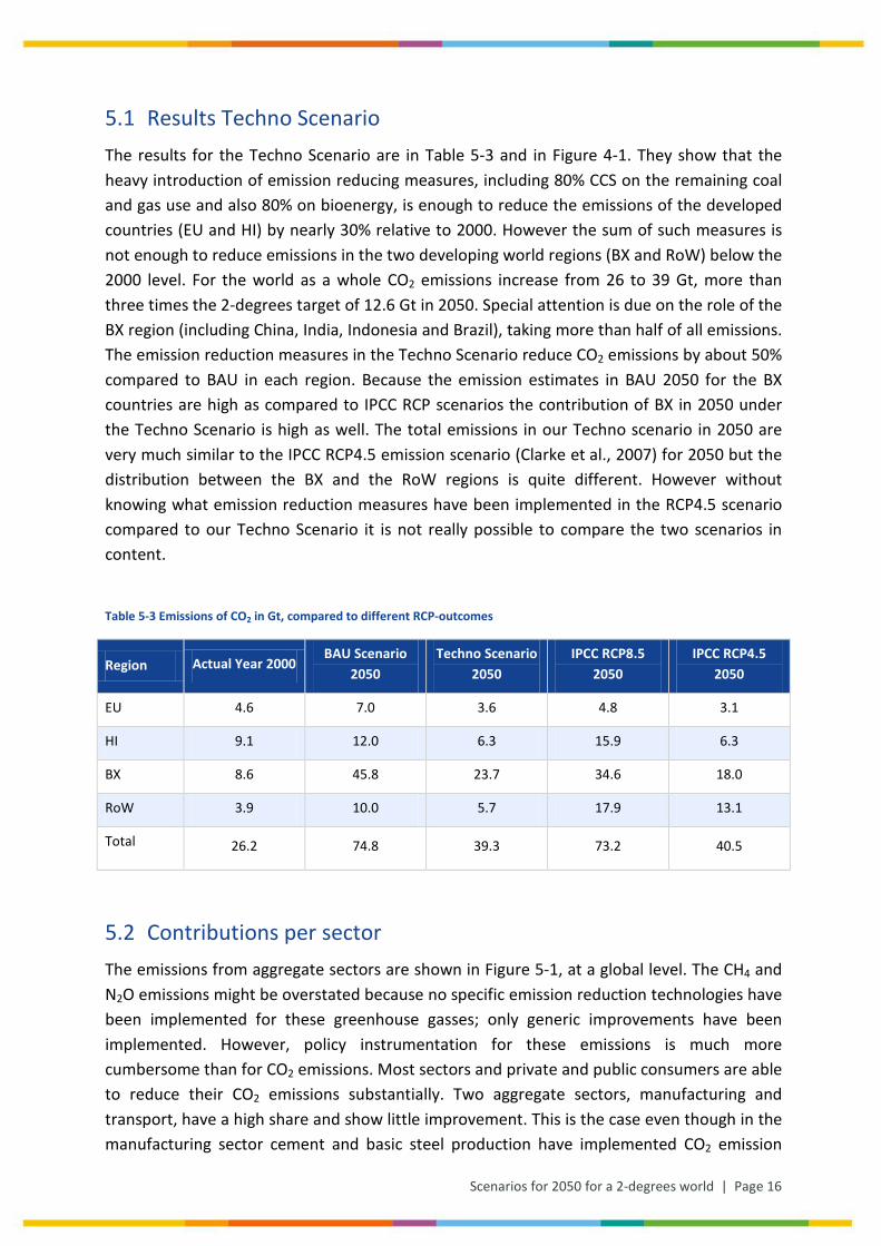
5.2 Contributions per sector The emissions from aggregate sectors are shown in Figure 5-1, at a global level. The CH4 and N2O emissions might be overstated because no specific emission reduction technologies have been implemented for these greenhouse gasses; only generic improvements have been implemented. However, policy instrumentation for these emissions is much more cumbersome than for CO2 emissions. Most sectors and private and public consumers are able to reduce their CO2 emissions substantially. Two aggregate sectors, manufacturing and transport, have a high share and show little improvement. This is the case even though in the manufacturing sector cement and basic steel production have implemented CO2 emission
Page 17 | Scenarios for 2050 for a 2-degrees world
reduction technology and in the transport sector land transport is now mostly based on electricity. The sheer demand growth annihilates the improvements. Where might be the most relevant options for further reduction?
Figure 5-1 Global aggregate sector emissions of CO2, CH4 and N2O
0.0
2.0
4.0
6.0
8.0
10.0
Gt C
O2
eq.
World, 2000CH4 + N2OCO2
0.0
5.0
10.0
15.0
20.0
25.0
30.0
Gt C
O2
eq.
BAU, 2050 CH4 + N2OCO2
0.0
5.0
10.0
15.0
20.0
25.0
Gt C
O2
eq
Techno, 2050 CH4 + N2O
CO2
Scenarios for 2050 for a 2-degrees world | Page 18
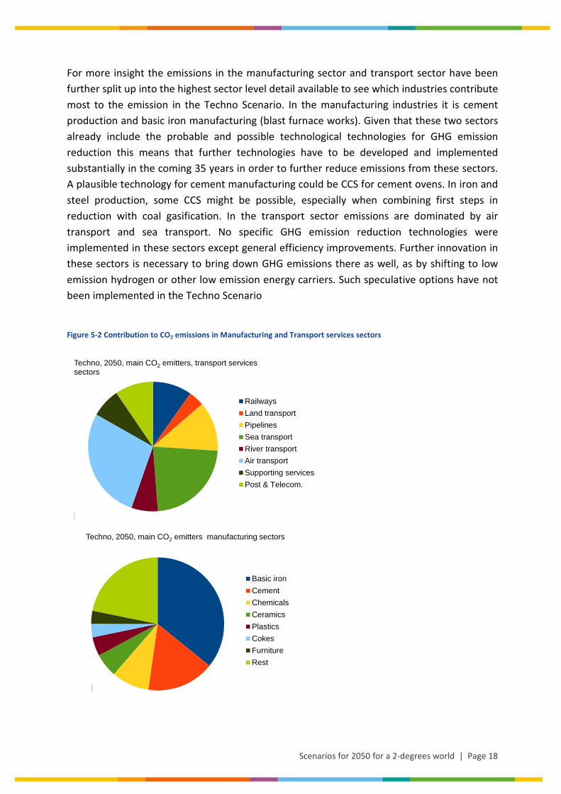
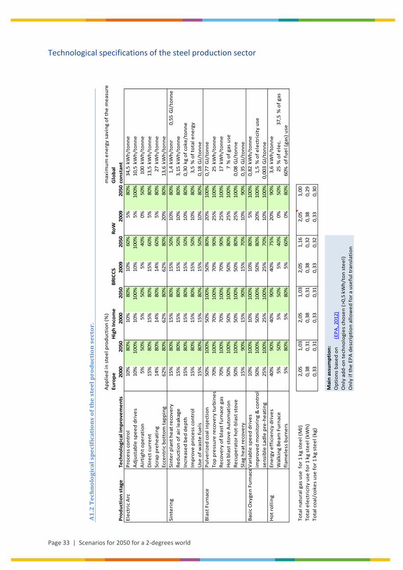
For more insight the emissions in the manufacturing sector and transport sector have been further split up into the highest sector level detail available to see which industries contribute most to the emission in the Techno Scenario. In the manufacturing industries it is cement production and basic iron manufacturing (blast furnace works). Given that these two sectors already include the probable and possible technological technologies for GHG emission reduction this means that further technologies have to be developed and implemented substantially in the coming 35 years in order to further reduce emissions from these sectors. A plausible technology for cement manufacturing could be CCS for cement ovens. In iron and steel production, some CCS might be possible, especially when combining first steps in reduction with coal gasification. In the transport sector emissions are dominated by air transport and sea transport. No specific GHG emission reduction technologies were implemented in these sectors except general efficiency improvements. Further innovation in these sectors is necessary to bring down GHG emissions there as well, as by shifting to low emission hydrogen or other low emission energy carriers. Such speculative options have not been implemented in the Techno Scenario
Figure 5-2 Contribution to CO2 emissions in Manufacturing and Transport services sectors
Techno, 2050, main CO2 emitters, transport services sectors
RailwaysLand transportPipelinesSea transportRiver transportAir transportSupporting servicesPost & Telecom.
Techno, 2050, main CO2 emitters manufacturing sectors
Basic ironCementChemicalsCeramicsPlasticsCokesFurnitureRest
Page 19 | Scenarios for 2050 for a 2-degrees world
6 Scenario 2050: Towards a 2-Degrees World scenario
After implementing all main probable and possible technological solutions for climate change emission mitigation, behavioural changes by consumers remain for a further emission reduction. Two types of behavioural changes have been investigated.
1. A shift from consumption of high carbon-intensive products (goods and services) like air travel to low carbon-intensive products, like music performance and theatre.
2. Reduced production and consumption, implying reduced economic growth.
We have not implemented these measures for their limited direct policy relevance, as they are far away from plausibility in terms of psychology and policy instrumentation. But we show what effects could be. Finally, we show how this scenario might be filled in normatively, either assuming an equal emission per capita or an equal emission per Euro GDP. Starting point for the analysis here is the Techno Scenario.
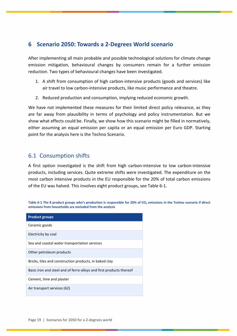
6.1 Consumption shifts A first option investigated is the shift from high carbon-intensive to low carbon-intensive products, including services. Quite extreme shifts were investigated. The expenditure on the most carbon intensive products in the EU responsible for the 20% of total carbon emissions of the EU was halved. This involves eight product groups, see Table 6-1.
Table 6-1 The 8 product groups who’s production is responsible for 20% of CO2 emissions in the Techno scenario if direct emissions from households are excluded from the analysis
Product groups
Ceramic goods
Electricity by coal
Sea and coastal water transportation services
Other petroleum products
Bricks, tiles and construction products, in baked clay
Basic iron and steel and of ferro-alloys and first products thereof
Cement, lime and plaster
Air transport services (62)
Scenarios for 2050 for a 2-degrees world | Page 20
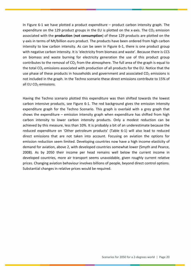
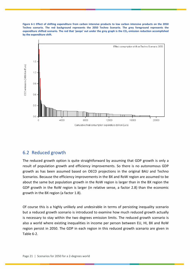
In Figure 6-1 we have plotted a product expenditure – product carbon intensity graph. The expenditure on the 129 product groups in the EU is plotted on the x-axis. The CO2 emission associated with the production (not consumption) of these 129 products are plotted on the y-axis in terms of Mt/billion euro product. The products have been ordered from high carbon intensity to low carbon intensity. As can be seen in Figure 6-1, there is one product group with negative carbon intensity. It is ‘electricity from biomass and waste’. Because there is CCS on biomass and waste burning for electricity generation the use of this product group contributes to the removal of CO2 from the atmosphere. The full area of the graph is equal to the total CO2 emissions associated with production of all products for the EU. Notice that the use phase of these products in households and government and associated CO2 emissions is not included in the graph. In the Techno scenario these direct emissions contribute to 15% of all EU CO2 emissions.
Having the Techno scenario plotted this expenditure was then shifted towards the lowest carbon intensive products, see Figure 6-1. The red background gives the emission intensity expenditure graph for the Techno Scenario. This graph is overlaid with a grey graph that shows the expenditure – emission intensity graph when expenditure has shifted from high carbon intensity to lower carbon intensity products. Only a modest reduction can be achieved by this measure, less than 10%. It is probably a bit of an underestimate because the reduced expenditure on ‘Other petroleum products’ (Table 6-1) will also lead to reduced direct emissions that are not taken into account. Focusing on aviation the options for emission reduction seem limited. Developing countries now have a high income elasticity of demand for aviation, above 2, with developed countries somewhat lower (Smyth and Pearce, 2008). As by 2050 their income per head remains well below the current income in developed countries, more air transport seems unavoidable, given roughly current relative prices. Changing aviation behaviour involves billions of people, beyond direct control options. Substantial changes in relative prices would be required.
Page 21 | Scenarios for 2050 for a 2-degrees world
Figure 6-1 Effect of shifting expenditure from carbon intensive products to low carbon intensive products on the 2050 Techno scenario. The red background represents the 2050 Techno Scenario. The grey foreground represents the expenditure shifted scenario. The red that ‘peeps’ out under the grey graph is the CO2 emission reduction accomplished by the expenditure shift.
6.2 Reduced growth The reduced growth option is quite straightforward by assuming that GDP growth is only a result of population growth and efficiency improvements. So there is no autonomous GDP growth as has been assumed based on OECD projections in the original BAU and Techno Scenarios. Because the efficiency improvements in the BX and RoW region are assumed to be about the same but population growth in the RoW region is larger than in the BX region the GDP growth in the RoW region is larger (in relative sense, a factor 2.8) than the economic growth in the BX region (a factor 1.8).
Of course this is a highly unlikely and undesirable in terms of persisting inequality scenario but a reduced growth scenario is introduced to examine how much reduced growth actually is necessary to stay within the two degrees emission limits. The reduced growth scenario is also a world where existing inequalities in income per person between EU, HI, BX and RoW region persist in 2050. The GDP in each region in this reduced growth scenario are given in Table 6-2.
Scenarios for 2050 for a 2-degrees world | Page 22
Table 6-2 GDP growth, growth factor and growth reduction assumption
Region GDP 2000
Billion Euro
GDP 2050 TS
Billion Euro
2050 TS reduced Growth
Billion Euro
Growth factor relative to 2000
Growth reduction relative to TS.
EU 8.4 19.3 11.2 1.33 0.58
HI 18.1 36.6 27.5 1.52 0.75
BX 3.8 37.2 6.8 1.76 0.18
RoW 3.6 16.2 10.2 2.79 0.65
Total 34.0 109.3 55.7 1.64 0.52
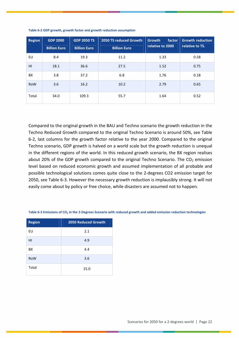
Compared to the original growth in the BAU and Techno scenario the growth reduction in the Techno Reduced Growth compared to the original Techno Scenario is around 50%, see Table 6-2, last columns for the growth factor relative to the year 2000. Compared to the original Techno scenario, GDP growth is halved on a world scale but the growth reduction is unequal in the different regions of the world. In this reduced growth scenario, the BX region realises about 20% of the GDP growth compared to the original Techno Scenario. The CO2 emission level based on reduced economic growth and assumed implementation of all probable and possible technological solutions comes quite close to the 2-degrees CO2 emission target for 2050, see Table 6-3. However the necessary growth reduction is implausibly strong. It will not easily come about by policy or free choice, while disasters are assumed not to happen.
Table 6-3 Emissions of CO2 in the 2-Degrees Scenario with reduced growth and added emission reduction technologies
Region 2050 Reduced Growth
EU 2.1
HI 4.9
BX 4.4
RoW 3.6
Total 15.0
Page 23 | Scenarios for 2050 for a 2-degrees world
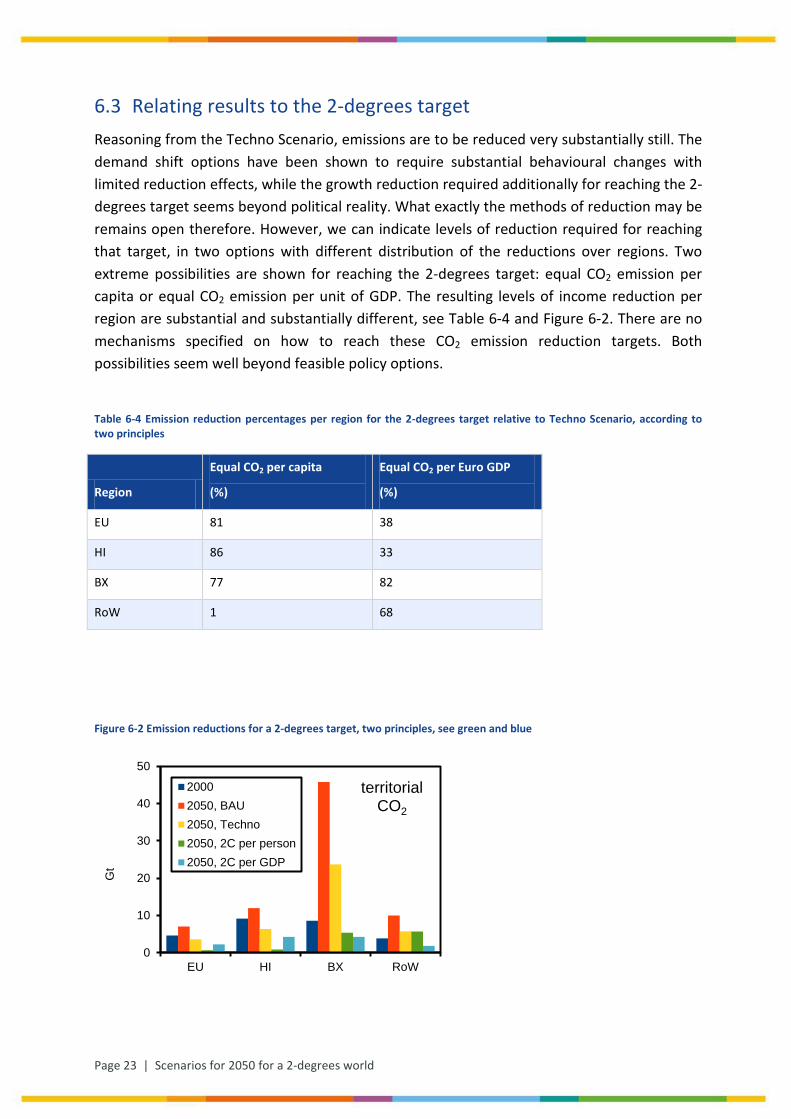
6.3 Relating results to the 2-degrees target Reasoning from the Techno Scenario, emissions are to be reduced very substantially still. The demand shift options have been shown to require substantial behavioural changes with limited reduction effects, while the growth reduction required additionally for reaching the 2-degrees target seems beyond political reality. What exactly the methods of reduction may be remains open therefore. However, we can indicate levels of reduction required for reaching that target, in two options with different distribution of the reductions over regions. Two extreme possibilities are shown for reaching the 2-degrees target: equal CO2 emission per capita or equal CO2 emission per unit of GDP. The resulting levels of income reduction per region are substantial and substantially different, see Table 6-4 and Figure 6-2. There are no mechanisms specified on how to reach these CO2 emission reduction targets. Both possibilities seem well beyond feasible policy options.
Table 6-4 Emission reduction percentages per region for the 2-degrees target relative to Techno Scenario, according to two principles
Region
Equal CO2 per capita
(%)
Equal CO2 per Euro GDP
(%)
EU 81 38
HI 86 33
BX 77 82
RoW 1 68
Figure 6-2 Emission reductions for a 2-degrees target, two principles, see green and blue
0
10
20
30
40
50
EU HI BX RoW
Gt
territorialCO2
20002050, BAU2050, Techno2050, 2C per person2050, 2C per GDP
Scenarios for 2050 for a 2-degrees world | Page 24
6.4 Conclusions on 2-Degrees Scenario The overall conclusion here is that the quite extreme technical measures in the Techno Scenario are not enough to reduce emissions to the 2-degrees target level. Adding substantial shifts in consumption structure is by far not enough to get to the 2-degrees target. Though emissions per unit of GDP have been reduced substantially, the sheer level of economic growth supersedes these improvements. Under current assumptions, the 2-degrees target may only be reached by adding extreme reductions in economic growth or by introducing novel technologies with extremely low emissions per unit of GDP.
Page 25 | Scenarios for 2050 for a 2-degrees world
7 Discussion
7.1 Overall reasonableness of outcomes The world increasingly will start to look like developed countries are now. A two-fold rise in GDP of developed countries by 2050 implies a growth rate of around 1.4%. A 10-fold rise in 2050 GDP in emerging countries relative to 2000 implies a growth rate of around 5%. In the rest of the world the growth rate is assumed to be around 3%. These growth rates seem well in the range of the feasible. For some specific sectors and technologies growth rates will be much higher. For a substantial electrification in transport and heating, resource use may become a bottleneck. For copper for example, growth rates in the order of 7% would be needed, substantially higher than the 5% realized in the last half century. Production would have to double every 10 years, from 14 years in the last half century. For such increases long term planning is required, based on trustable climate policy inducing the electrification. Here we abstract from such constraints.
Land-use issues might come up in unexpected ways, due to substantial intensification with higher also GHG emissions and loss of nature area. These ecological risks need substantial attention but have been assumed here to be manageable. Such issues have been left out of account now.
International trade may also have hidden problems. Though not rising as a percentage of global GDP, the sheer growth of global GDP may require too large volumes of trade to effectively handle in the sea lanes and the expanded ports available.
As to the discussion on the 2-degrees scenario, the composition of final demand may not be shiftable as assumed in chapter 6, and even then has limited effects. For such an analysis, essential for policy purposes, additional information is required, as on price elasticity and income elasticity of specific expenditures. The shifts required will very much depend on the instrumentation of climate policy. Here only the task ahead is shown.
A final deep underlying assumption is that we will not have global collapses, as through world wars, pandemics or other disasters.
Scenarios for 2050 for a 2-degrees world | Page 26
7.2 Changing assumptions There are always good reasons to change assumptions, adding reasoning on mechanisms behind future developments. Simplifying assumptions as used here may be refined, showing the influence of refining. For example, the growth of some key sectors and consumption activities will approach saturation. With rising incomes several production and consumption activities level off: their income elasticity of demand goes down. This holds for most travelling including person car transport (Goodwin, 2012) and for living space per person (Hu et al., 2010). For transport infrastructure the volume reductions as indicated by Goodwin would follow logically. For other built infrastructure levelling off seems most probable as well when final demand shifts to services. Most developing countries, however, have still to build up their infrastructure, like roads and railroads, which then have a very long life time. Also for many durable consumer goods this levelling off relation to income per head holds. One washing and drying machine per household will mostly suffice. Such a detailed analysis would support specific changes in final demand, and corresponding changes in production volumes. It would require substantial additional information, translated into further assumptions. One main additional assumption then would be on how the income not spent is redistributed over other activities.
Page 27 | Scenarios for 2050 for a 2-degrees world
8 Interpretation and conclusions
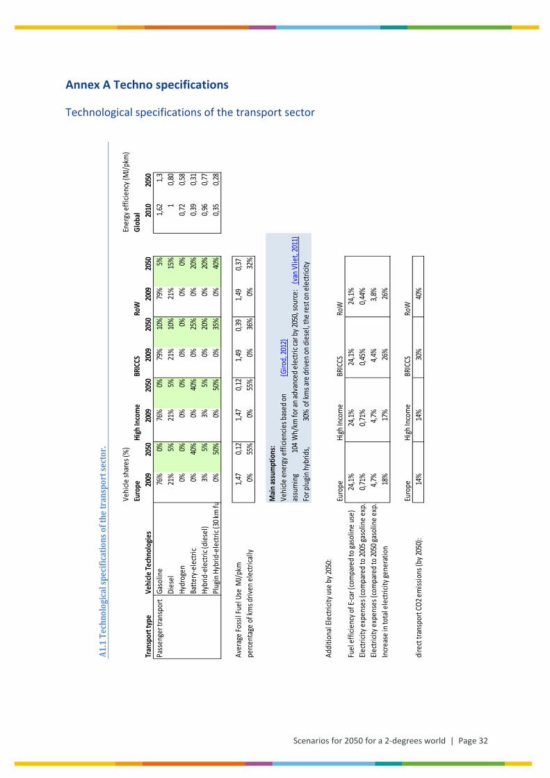
8.1 Prediction versus goal oriented scenario analysis Though technologies and expenditures have been specified in detail, they should not be seen as predictions but only as technical options, required to give specificity in the scenarios. We have taken electric cars as the dominant drive mode but it might as well be hydrogen or ammonia as a fuel, linked to an electric drive, or to other drive systems. It is the nature of the change that counts: a full shift in drive mode is required, away from de-central carbon emissions. The technologies resulting will be efficient in some way, as costs are a main selection mechanism. So our efficient electric drives are exemplary, not predictive. Any transport drive system should be (near) zero direct emission, as otherwise CO2 emissions from transport would remain too high: CCS on decentralized mobile emitters just is not possible. Biomass for energy has been moved fully to electricity generation with CCS.
8.2 Price and income effects One of the important limitations of the use of a static model is that it does not capture secondary effects. Secondary effects – for example relative price and income effects – may have consequences on emissions. Our model might therefore be judged as having high estimates of emissions for a given scenario assumption. On the other hand we force our model to reproduce the reasonable assumptions on GDP growth by the OECD. While it is for certain that scenario assumptions have income effects the total of all income effects should result in the GDP scenarios of the OECD and our model complies to that.
8.3 Comparison with other scenario studies The Techno Scenario is in the middle domain of the scenarios linked to a substantial warming by 2100. The 2-Degrees Scenario relates to the RCP2.6 scenario, where there are very limited scenarios studies available. Getting towards a 2-degrees target may involve not so plausible socio-economic scenarios. Getting there in terms of the IO-scenario presented here involves ultimately a drastic assumption: limiting economic growth by about 50%. This is much higher than other studies have so far reported. Knopf et al. (2009) and Edenhofer et al. (2009) have for example reported a GDP decrease between 2,5% and 5%, due to climate policy measures. Such minor reductions relate more to cost of climate policy than to an active reduction of economic growth as a means for emission reduction.
Scenarios for 2050 for a 2-degrees world | Page 28
One of the essential assumptions underlying the different 2-degree scenario outcomes is the elaboration of the shift from the primary to the secondary and tertiary sectors. We assume that at a global level such a shift is not possible, due to the still limited development stage of the developing countries in 2050. Several integrated assessment models implicitly assume a development in industrial energy intensity similar to historic trends in developed countries through energy intensity curves. Without suggesting a preference for any type of modelling, this study shows that the difference in outcomes of climate policy cost predictions, emerging from such implicit modelling assumptions, may be very large.
8.4 Conclusions The main conclusion is that reaching a 2-degrees target is possible only with deep changes in technology and deep changes in consumption and reduced growth levels. Technology alone will not do it and behavioural change alone cannot do either. Shifts In consumption can only have a limited influence on carbon emissions. A reduced growth scenario compatible with a 2 degrees target would be so drastic that it is not feasible and would persist the income differences between poor and rich countries.
Transforming both production and consumption in a globalized market economy would require a substantial use of the price mechanism: carbon pricing is essential. The thus adapted neoliberal order will not suffice, as markets have a limited domain. The long term technology development as is needed will require substantial public action. Also infrastructure development is done or guided by public government. Saddle points and lock-ins are to be resolved with specific actions. Missing and distorted markets are to be replaced or repaired. How exactly this is to be done, with which set of instruments does not follow from this scenario analysis. This analysis shows however that there is a dramatic task ahead for global and regional climate policy, with high demands on very broadly working instruments.
Page 29 | Scenarios for 2050 for a 2-degrees world
9 References
Clarke, L., J. Edmonds, H. Jacoby, H. Pitcher, J. Reilly, R. Richels (2007) Scenarios of Greenhouse Gas Emissions and Atmospheric Concentrations. Sub-report 2.1A of Synthesis and Assessment Product 2.1 by the U.S. Climate Change Science Program and the Subcommittee on Global Change Research. Department of Energy, Office of Biological & Environmental Research, Washington, 7 DC., USA, 154 pp.
Vassilis Daioglou, Bas J. van Ruijven, Detlef P. van Vuuren, Model projections for household energy use in developing countries, Energy, Volume 37, Issue 1, January 2012, Pages 601-615,
Edenhofer, O., C. Carraro, J-C. Hourcade, K. Neuhoff, G. Luderer, C. Flachsland, M. Jakob, A. Popp, J. Steckel, J. Strohschein, N. Bauer, S. Brunner, M. Leimbach, H. Lotze-Campen, V. Bosetti, E. de Cian, M. Tavoni, O. Sassi, H. Waisman, R. Crassous-Doerfler, S. Monjon, S. Dröge, H. van Essen, P. del Río and A. Türk (2009) The economics of decarbonization. Report of the RECIPE project, Potsdam Institute for Climate Impact Research, Potsdam.
EPA (2000) Energy Cost and IAQ Performance of Ventilation Systems and Controls.
EPA (2010) Available and Emerging Technologies for Reducing Greenhouse Gas Emissions from the Portland Cement Industry.
EPA (2012) Available and Emerging Technologies for Reducing Greenhouse Gas Emissions from the Iron and Steel Industry.
Eurostat (2008) Eurostat Manual of Supply, Use and Input-Output Tables, Luxembourg: Office for Official Publications of the European Communities, ISBN 978-92-79-04735-0, ISSN 1977-0375.
Girod B., D.P. van Vuuren, S. Deetman (2012) Global travel within the 2°C climate target, Energy Policy, Volume 45, June 2012, Pages 152-166.
Goodwin, P. (2012) Peak Travel, Peak Car and the Future of Mobility: Evidence, Unresolved Issues, Policy Implications, and a Research Agenda. OECD Discussion Paper No. 2012-13. Prepared for the Roundtable on Long-Run Trends in Travel Demand 29-30 November 2012
Hourcade, J.-C., R. Crassous & O. Sassi (2006) Endogenous structural change and climate targets: Modelling experiments with IMACLIM-R. The Energy Journal 27(special issue no 1.) 259-276.
Hu, M., H. Bergsdal, E. van der Voet, G. Huppes & D.B. Müller (2010) Dynamics of urban and rural housing stocks in China. Building Research and Information 38(3):301-317.
Huppes, G., Koning A. de, Suh S., Heijungs R. ,Van Oers L., Nielsen P., Guinée J.B. (2006). Environmental impacts of consumption in the European Union: High-resolution input-output tables with detailed environmental extensions. Journal of Industrial Ecology10(3): 129-146.
IEA (2013) World Model Documentation, 2013 version.
Jakeman and Fisher (2010) Benefits of Multi-Gas Mitigation: An Application of the Global Trade and Environment Model (GTEM), 2006 updated 2010. A chapter in: EMF 21 Multi-Greenhouse Gas Mitigation and Climate Policy” (eds. F.C. De La Chesnaye & John P. Weyant).
Scenarios for 2050 for a 2-degrees world | Page 30
Jordan, Andrew, Tim Rayner, Heike Schroeder, Neil Adger, Kevin Anderson, Alice Bows, Corinne Le Quéré, Manoj Joshi, Sarah Mander, Nem Vaughan & Lorraine Whitmarsh (2013) Going beyond two degrees? The risks and opportunities of alternative options, Climate Policy, 13:6, 751-769, DOI: 10.1080/14693062.2013.835705
Junius, T and J. Oosterhaven (2003) The solution of updating or regionalizing a matrix with both positive and negative entries. Economic Systems Research 15(1)87-96.
Knopf, B. and O. Edenhofer, T. Barker, N. Bauer, L. Baumstark, B. Chateau, P. Criqui, A. Held, M. Isaac, M. Jakob, E. Jochem, A. Kitous, S. Kypreos, M. Leimbach, B. Magné, S. Mima, W. Schade, S. Scrieciu, H. Turton and D. van Vuuren (2009) “The economics of low stabilisation: implications for technological change and policy”, Chapter 11 in Making Climate Change Work for Us (eds. M. Hulme and H Neufeldt), Cambridge University Press, Cambridge, UK.
Konijn P.J.A. (1994) The make and use of commodities by industries. On the compilation of input-output data from the national accounts. Universiteit Twente, Enschede.
Kramer G.J., M. Haigh (2009) No quick switch to low-carbon energy. Nature, 462 (7273)568–569.
Lucas, Paul L.; Vuuren, D.P. van; Olivier, J.G.J.; Elzen, M.G.J. den (2007) Long-term reduction potential of non-CO2 greenhouse gases. Environmental Science & Policy, 10(2)85 - 103.
Marcel P. Timmer (ed) (2012), The World Input-Output Database (WIOD): Contents, Sources and Methods, WIOD Working Paper Number 10.
Meinshausen, M., S. J. Smith, K. Calvin, J. S. Daniel, M. L. T. Kainuma, J-F. Lamarque, K. Matsumoto, S. A. Montzka, S. C. B. Raper, K. Riahi, A. Thomson, G. J. M. Velders, D.P. van Vuuren (2011) The RCP GHG concentrations and their extension from 1765 to 2300, Climatic Change 109(1-2)213–241.
MNP (2006). Integrated modelling of global environmental change. An overview of IMAGE 2.4.Bilthoven. Netherlands Environmental Assessment Agency
Morna Isaac, Detlef P. van Vuuren (2009) Modeling global residential sector energy demand for heating and air conditioning in the context of climate change, Energy Policy, Volume 37, Issue 2, Pages 507-521,
Moss, R.,H., Edmonds, J.,A., Hibbard, K.,A., Manning, M.,R., Rose, S.,K., van Vuuren, D.,P.,, Carter, T.,R., Emori, S., Kainuma, M., Kram, T., Meehl, G.,A., Mitchell, J.,F., Nakicenovic, N., Riahi, K., Smith, S.,J., Stouffer, R.,J., Thomson, A.,M., Weyant, J.,P., Wilbanks, T.,J. (2010). The next generation of scenarios for climate change research and assessment. Nature. 463(7282):747-56.
NETL (2010) Cost and Performance Baseline for Fossil Energy Plants Volume 1: Bituminous Coal and Natural Gas to Electricity Report of the National Energy Technology Laboratory.
OECD (2012a) OECD Environmental Outlook to 2050: The consequences of inaction, OECD publishing.
OECD (2012b), Looking to 2060: A Global Vision of Long-Term Growth, OECD Economics Department Policy Notes, No. 15 November 2012.
Riahi, K., Gruebler, A. and Nakicenovic N. (2007) Scenarios of long-term socio-economic and environmental development under climate stabilization. Technological Forecasting and Social Change 74, 7, 887-935.
Smyth, M. and Pearce, B. (2008) Air travel demand. IATA Economics Briefing No 9: IATA, April 2008. Downloadable at: http://www.iata.org/whatwedo/Documents/economics/air_travel_demand.pdf
Page 31 | Scenarios for 2050 for a 2-degrees world
Strømman,, A.H., Hertwich, E.G., Duchin, F. (2009) Shifting Trade Patterns as a Means of Reducing Global Carbon Dioxide Emissions, A Multi-objective Analysis. Journal of Industrial Ecology Vol. 13-1, pp38–57.
Timmer M.P. (ed.) (2012) The World Input-Output Database (WIOD): Contents, Sources and Methods,WIOD Working Paper Number 10
Tukker, A., G. Huppes, J.B. Guinée, R. Heijungs, A. de Koning, L. van Oers, S. Suh, T. Geerken, M. Van Holderbeke, B. Jansen and P. Nielsen (2006) Environmental Impacts of Products (EIPRO) - Analysis of the life cycle environmental impacts related to the final consumption of the EU-25. European Commission, Joint Research Centre (DG JRC), Institute for Prospective Technological Studies. EU Report No 22284EN, ISBN 92-79-02361-6.
Tukker A., Koning A. de, Wood R., Hawkins T., Lutter S., Acosta J., Rueda Cantuche J.M., Bouwmeester M.C., Oosterhaven J., Drosdowski T. & Kuenen J.(2013) EXIOPOL – Development and illustrative analyses of a detailed global mr eeSUT/IOT. Economic Systems Research25(1): 50-70.
Vliet, J. van, M.G.J. den Elzen, D.P. van Vuuren (2009) Meeting radiative forcing targets under delayed participation. Energy Economics 31, 152-162.
Oscar van Vliet, Anne Sjoerd Brouwer, Takeshi Kuramochi, Machteld van den Broek, André Faaij, Energy use, cost and CO2 emissions of electric cars, Journal of Power Sources, Volume 196, Issue 4, 15 February 2011, Pages 2298-2310,
Vuuren, D.P. van, E. Stehfest, M.G.J. den Elzen, T. Kram, J. van Vliet, S. Deetman, M. Isaac, K.K. Goldewijk, A. Hof, A. Mendoza Beltran, R. Oostenrijk, B. van Ruijven (2011). RCP2.6: exploring the possibility to keep global mean temperature increase below 2°C. Climatic Change 109(1-2): 95-116
Worrell E., N. Martin, L. Price, Potentials for energy efficiency improvement in the US cement industry, Energy, Volume 25, Issue 12, December 2000, Pages 1189-1214,
Scenarios for 2050 for a 2-degrees world | Page 32
Annex A Techno specifications
Technological specifications of the transport sector
A1.1
Tec
hnol
ogica
l spe
cifica
tions
of t
he tr
ansp
ort s
ecto
r.
Vehi
cle sh
ares
(%)
Ener
gy ef
ficie
ncy (
MJ/p
km)
Euro
peHi
gh In
com
eBR
ICCS
RoW
Glob
alTr
ansp
ort t
ype
Vehi
cle Te
chno
logie
s20
0920
5020
0920
5020
0920
5020
0920
5020
1020
50Pa
ssen
ger t
rans
port
Gaso
line
76%
0%76
%0%
79%
10%
79%
5%1,6
21,3
Dies
el21
%5%
21%
5%21
%10
%21
%15
%1
0,80
Hydr
ogen
0%0%
0%0%
0%0%
0%0%
0,72
0,58
Batte
ry-e
lectr
ic0%
40%
0%40
%0%
25%
0%20
%0,3
90,3
1Hy
brid
-ele
ctric
(die
sel)
3%5%
3%5%
0%20
%0%
20%
0,96
0,77
Plug
in H
ybrid
-ele
ctric
(30 k
m fu
0%50
%0%
50%
0%35
%0%
40%
0,35
0,28
Aver
age F
ossil
Fuel
Use
MJ/p
km1,4
70,1
21,4
70,1
21,4
9
0,39
1,4
9
0,37
pe
rcent
age o
f km
s driv
en el
ectri
cally
0%55
%0%
55%
0%36
%0%
32%
Main
assu
mpt
ions
:Ve
hicle
ener
gy ef
ficie
ncie
s bas
ed on
(Giro
d, 20
12)
assu
min
g 10
4W
h/km
for a
n adv
ance
d ele
ctric
car b
y 205
0, so
urce
: (v
an V
liet,
2011
)Fo
r plu
gin hy
brid
s,30
%of
kms a
re dr
iven o
n die
sel, t
he re
st on
elec
tricit
y
Addi
tiona
l Ele
ctrici
ty us
e by 2
050:
Euro
peHi
gh In
com
eBR
ICCS
RoW
Fuel
effic
ienc
y of E
-car (
com
pare
d to g
asol
ine u
se)
24,1%
24,1%
24,1%
24,1%
Electr
icity
expe
nses
(com
pare
d to 2
005 g
asol
ine e
xp.)
0,71%
0,71%
0,45%
0,44%
Electr
icity
expe
nses
(com
pare
d to 2
050 g
asol
ine e
xp.)
4,7%
4,7%
4,4%
3,8%
Incre
ase i
n tot
al el
ectri
city g
ener
atio
n18
%17
%26
%26
%
Euro
peHi
gh In
com
eBR
ICCS
RoW
dire
ct tra
nspo
rt CO
2 em
issio
ns (b
y 205
0):
14%
14%
30%
40%
Page 33 | Scenarios for 2050 for a 2-degrees world
Technological specifications of the steel production sector
A1.
2 T
echn
olog
ical
spe
cifi
cati
ons
of th
e st
eel p
rodu
ctio
n se
ctor
.
App
lied
in s
teel
pro
duct
ion
(%)
max
imum
ene
rgy
savi
ng o
f the
mea
sure
Euro
peH
igh
Inco
me
BRIC
CSRo
WG
loba
lPr
oduc
tion
sta
geTe
chno
logi
cal i
mpr
ovem
ents
2000
2050
2000
2050
2009
2050
2009
2050
cons
tant
Elec
tric
Arc
Proc
ess
cont
rol
10%
80%
10%
80%
10%
60%
5%80
%34
,5kW
h/to
nne
Adj
usta
ble
spee
d dr
ives
10%
100%
10%
100%
10%
100%
5%10
0%10
,5kW
h/to
nne
Air
tigh
t ope
rati
on5%
50%
5%50
%5%
40%
0%50
%10
0kW
h/to
nne
Dir
ect c
urre
nt15
%80
%15
%80
%15
%60
%5%
80%
13,5
kWh/
tonn
eSc
rap
preh
eati
ng14
%80
%14
%80
%14
%60
%5%
80%
27kW
h/to
nne
Ecce
ntri
c bo
ttom
tapp
ing
62%
80%
62%
80%
62%
80%
20%
80%
13,6
kWh/
tonn
eSi
nter
ing
Sint
er p
lant
hea
t rec
over
y15
%80
%15
%80
%15
%50
%10
%80
%1,
4kW
h/to
nn0,
55G
J/to
nne
Redu
ctio
n of
air
leak
age
15%
80%
15%
80%
15%
50%
10%
80%
3,15
kWh/
tonn
eIn
crea
sed
bed
dept
h15
%80
%15
%80
%15
%50
%10
%80
%0,
30kg
of c
oke/
tonn
eIm
prov
e pr
oces
s co
ntro
l15
%80
%15
%80
%15
%50
%10
%80
%3,
5%
of t
otal
ene
rgy
Use
of w
aste
fuel
s15
%80
%15
%80
%15
%50
%10
%80
%0,
18G
J/to
nne
Blas
t Fur
nace
Pulv
eriz
ed c
oal i
njec
tion
50%
100%
50%
100%
50%
80%
20%
100%
0,77
GJ/
tonn
e To
p pr
essu
re re
cove
ry tu
rbin
es
70%
100%
70%
100%
70%
90%
25%
100%
25kW
h/to
nne
Reco
very
of b
last
furn
ace
gas
70%
100%
70%
100%
70%
90%
25%
100%
17kW
h/to
nne
Hot
bla
st s
tove
Aut
omat
ion
50%
100%
50%
100%
50%
80%
25%
100%
7%
of g
as u
seRe
cupe
rato
r hot
-bla
st s
tove
50%
100%
50%
100%
50%
80%
25%
100%
0,08
GJ/
tonn
e Sl
ag h
eat r
ecov
ery
15%
90%
15%
90%
15%
70%
10%
90%
0,35
GJ/
tonn
e Ba
sic
Oxy
gen
Furn
ace
Var
iabl
e sp
eed
driv
es10
%10
0%10
%10
0%10
%80
%5%
100%
0,82
kWh/
tonn
eim
prov
ed m
onit
orin
g &
con
trol
50%
100%
50%
100%
50%
80%
20%
100%
1,5
% o
f ele
ctri
city
use
sens
ible
Lad
le p
re-h
eati
ng25
%10
0%25
%10
0%25
%70
%10
%10
0%0,
003
GJ/
tonn
eH
ot ro
lling
Ener
gy e
ffic
ienc
y dr
ives
40%
90%
40%
90%
40%
75%
20%
90%
3,6
kWh/
tonn
eW
alki
ng B
eam
Fur
nace
5%50
%5%
50%
5%40
%0%
50%
25%
of e
lec.
37,5
% o
f gas
fl
amel
ess
burn
ers
5%80
%5%
80%
5%60
%0%
80%
60%
of fu
el (g
as) u
se
Tota
l nat
ural
gas
use
for
1 k
g st
eel (
MJ)
2,05
1,03
2,05
1,03
2,05
1,16
2,05
1,00
Tota
l ele
ctri
city
use
for 1
kg
stee
l (kW
h)0,
380,
310,
380,
310,
38
0,
32
0,
38
0,
29
To
tal c
oal/
coke
s us
e fo
r 1 k
g st
eel (
kg)
0,33
0,31
0,33
0,31
0,33
0,32
0,33
0,30
Mai
n as
sum
ptio
n:O
ptio
ns b
ased
on
(EPA
, 201
2)O
nly
add-
on te
chno
logi
es c
hose
n (>
0,5
kWh/
ton
stee
l)O
nly
if th
e EP
A d
escr
ipti
on a
llow
ed fo
r a u
sefu
l tra
nsla
tion
Scenarios for 2050 for a 2-degrees world | Page 34
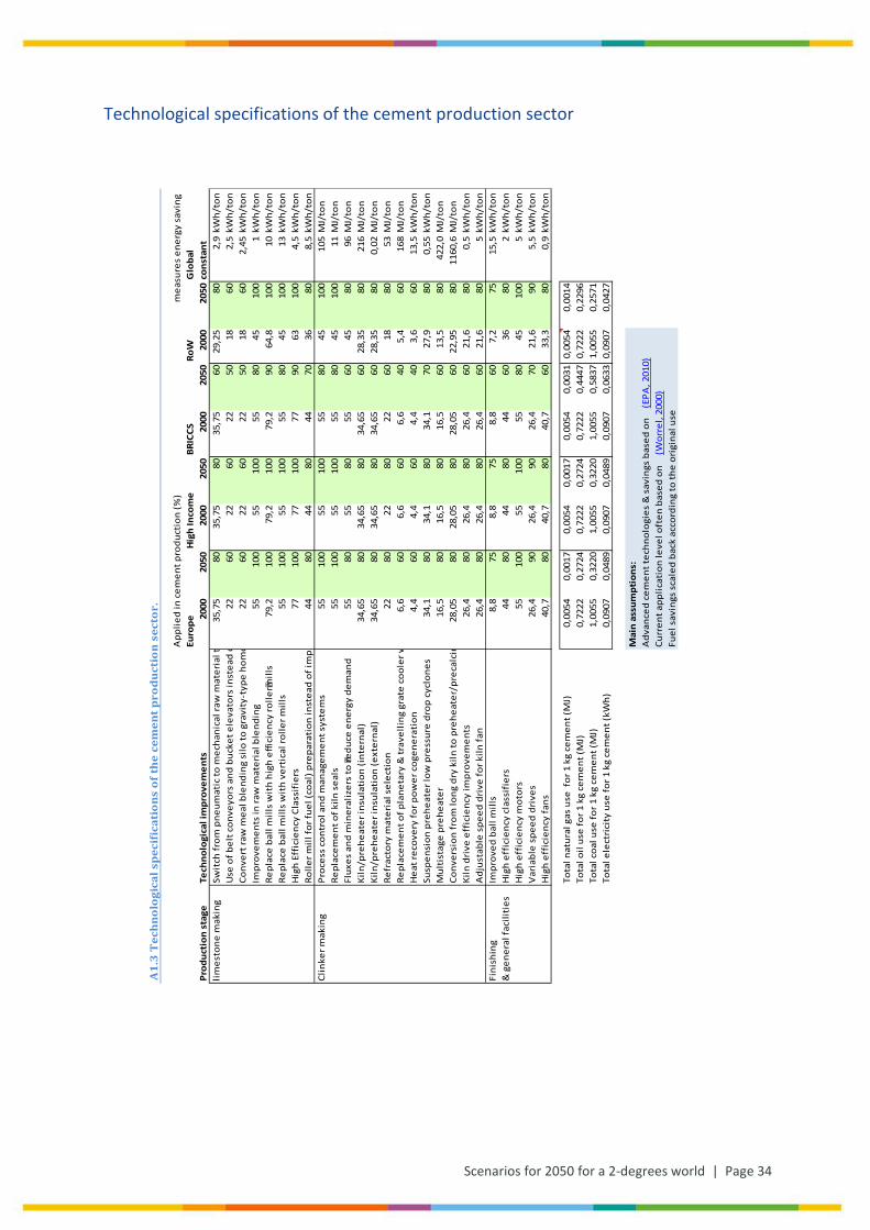
Technological specifications of the cement production sector
A1.
3 T
echn
olog
ical
spe
cifi
cati
ons
of th
e ce
men
t pro
duct
ion
sect
or.
App
lied
in c
emen
t pro
duct
ion
(%)
m
easu
res
ener
gy s
avin
g Eu
rope
Hig
h In
com
eBR
ICCS
RoW
Glo
bal
Prod
ucti
on s
tage
Tech
nolo
gica
l im
prov
emen
ts20
0020
5020
0020
5020
0020
5020
0020
50co
nsta
ntlim
esto
ne m
akin
gSw
itch
from
pne
umat
ic to
mec
hani
cal r
aw m
ater
ial t
35,7
580
35,7
580
35,7
560
29,2
580
2,9
kWh/
ton
Use
of b
elt c
onve
yors
and
buc
ket e
leva
tors
inst
ead
o
2260
2260
2250
1860
2,5
kWh/
ton
Conv
ert r
aw m
eal b
lend
ing
silo
to g
ravi
ty-t
ype
hom
o22
6022
6022
5018
602,
45kW
h/to
nIm
prov
emen
ts in
raw
mat
eria
l ble
ndin
g55
100
5510
055
8045
100
1kW
h/to
nRe
plac
e ba
ll m
ills
wit
h hi
gh e
ffici
ency
rolle
rmill
s79
,210
079
,210
079
,290
64,8
100
10kW
h/to
nRe
plac
e ba
ll m
ills
wit
h ve
rtic
al ro
ller m
ills
5510
055
100
5580
4510
013
kWh/
ton
Hig
h Ef
fici
ency
Cla
ssif
iers
7710
077
100
7790
6310
04,
5kW
h/to
nRo
ller m
ill fo
r fue
l (co
al) p
repa
rati
on in
stea
d of
impa
44
8044
8044
7036
808,
5kW
h/to
nCl
inke
r mak
ing
Proc
ess
cont
rol a
nd m
anag
emen
t sys
tem
s55
100
5510
055
8045
100
105
MJ/
ton
Repl
acem
ent o
f kiln
sea
ls55
100
5510
055
8045
100
11M
J/to
nFl
uxes
and
min
eral
izer
s to
redu
ce e
nerg
y de
man
d55
8055
8055
6045
8096
MJ/
ton
Kiln
/pre
heat
er in
sula
tion
(int
erna
l)34
,65
8034
,65
8034
,65
6028
,35
8021
6M
J/to
nKi
ln/p
rehe
ater
insu
lati
on (e
xter
nal)
34,6
580
34,6
580
34,6
560
28,3
580
0,02
MJ/
ton
Refr
acto
ry m
ater
ial s
elec
tion
2280
2280
2260
1880
53M
J/to
nRe
plac
emen
t of p
lane
tary
& tr
avel
ling
grat
e co
oler
w
6,6
606,
660
6,6
405,
460
168
MJ/
ton
Hea
t rec
over
y fo
r pow
er c
ogen
erat
ion
4,4
604,
460
4,4
403,
660
13,5
kWh/
ton
Susp
ensi
on p
rehe
ater
low
pre
ssur
e dr
op c
yclo
nes
34,1
8034
,180
34,1
7027
,980
0,55
kWh/
ton
Mul
tist
age
preh
eate
r16
,580
16,5
8016
,560
13,5
8042
2,0
MJ/
ton
Conv
ersi
on fr
om lo
ng d
ry k
iln to
pre
heat
er/p
reca
lcin
28
,05
8028
,05
8028
,05
6022
,95
8011
60,6
MJ/
ton
Kiln
dri
ve e
ffic
ienc
y im
prov
emen
ts26
,480
26,4
8026
,460
21,6
800,
5kW
h/to
nA
djus
tabl
e sp
eed
driv
e fo
r kiln
fan
26,4
8026
,480
26,4
6021
,680
5kW
h/to
nFi
nish
ing
Impr
oved
bal
l mill
s8,
875
8,8
758,
860
7,2
7515
,5kW
h/to
n&
gen
eral
faci
litie
sH
igh
effi
cien
cy c
lass
ifie
rs44
8044
8044
6036
802
kWh/
ton
Hig
h ef
fici
ency
mot
ors
5510
055
100
5580
4510
05
kWh/
ton
Var
iabl
e sp
eed
driv
es26
,490
26,4
9026
,470
21,6
905,
5kW
h/to
nH
igh
effi
cien
cy fa
ns40
,780
40,7
8040
,760
33,3
800,
9kW
h/to
n
Tota
l nat
ural
gas
use
for
1 k
g ce
men
t (M
J)0,
0054
0,00
170,
0054
0,00
170,
0054
0,00
310,
0054
0,00
14To
tal o
il us
e fo
r 1 k
g ce
men
t (M
J)0,
7222
0,27
240,
7222
0,27
240,
7222
0,44
470,
7222
0,22
96To
tal c
oal u
se fo
r 1 k
g ce
men
t (M
J)1,
0055
0,32
201,
0055
0,32
201,
0055
0,58
371,
0055
0,25
71To
tal e
lect
rici
ty u
se fo
r 1 k
g ce
men
t (kW
h)0,
0907
0,04
890,
0907
0,04
890,
0907
0,06
330,
0907
0,04
27
Mai
n as
sum
ptio
ns:
Adv
ance
d ce
men
t tec
hnol
ogie
s &
sav
ings
bas
ed o
n(E
PA, 2
010)
Curr
ent a
pplic
atio
n le
vel o
ften
bas
ed o
n(W
orre
l, 20
00)
Fuel
sav
ings
sca
led
back
acc
ordi
ng to
the
orig
inal
use
Page 35 | Scenarios for 2050 for a 2-degrees world
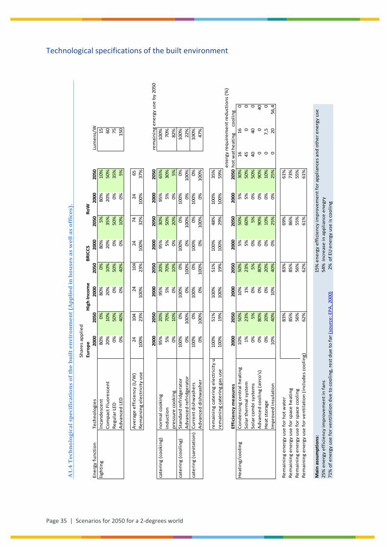
Technological specifications of the built environment
A1.
4 T
echn
olog
ical
spe
cifi
cati
ons
of th
e bu
ilt e
nvir
onm
ent (
App
lied
in h
ouse
s as
wel
l as
offi
ces)
.
Shar
es a
pplie
dEu
rope
Hig
h In
com
eBR
ICCS
RoW
Ener
gy fu
ncti
onTe
chno
logi
es20
0020
5020
0020
5020
0020
5020
0020
50Lu
men
s/W
light
ing
Inca
ndes
cent
80%
0%80
%0%
80%
5%80
%10
%15
Com
pact
Flu
ores
cent
20%
10%
20%
10%
20%
35%
20%
50%
60Re
gula
r LED
0%50
%0%
50%
0%50
%0%
35%
75A
dvan
ced
LED
0%40
%0%
40%
0%10
%0%
5%15
0
Ave
rage
eff
icie
ncy
(L/W
)24
10
4
24
104
24
74
24
65
Rem
aini
ng e
lect
rici
ty u
se10
0%23
%10
0%23
%10
0%32
%10
0%37
%
2000
2050
2000
2050
2000
2050
2000
2050
rem
aini
ng e
nerg
y us
e by
205
0ca
teri
ng (c
ooki
ng)
norm
al c
ooki
ng95
%20
%95
%20
%95
%30
%95
%65
%10
0%in
duct
ion
5%70
%5%
70%
5%50
%5%
30%
70%
pres
sure
coo
king
0%10
%0%
10%
0%20
%0%
5%82
%ca
teri
ng (c
oolin
g)St
anda
rd re
frid
gera
tor
100%
0%10
0%0%
100%
0%10
0%0%
100%
Adv
ance
d re
frid
gera
tor
0%10
0%0%
100%
0%10
0%0%
100%
22%
cate
ring
(san
itat
ion)
Curr
ent d
ishw
ashe
rs10
0%0%
100%
0%10
0%0%
100%
0%10
0%A
dvan
ced
dish
was
her
0%10
0%0%
100%
0%10
0%0%
100%
47%
rem
aini
ng c
ater
ing
elec
tric
ity
us10
0%51
%10
0%51
%10
0%48
%10
0%35
%re
mai
ning
cat
erin
g ga
s us
e10
0%19
%10
0%19
%10
0%29
%10
0%59
%en
ergy
requ
irem
ent r
educ
tion
s (%
)Ef
fici
ency
mea
sure
s20
0020
5020
0020
5020
0020
5020
0020
50ho
t wat
heat
ing
cool
ing
Hea
ting
/coo
ling
Cond
ensi
ng c
entr
al h
eati
ng10
%50
%10
%50
%5%
50%
5%30
%16
160
Sola
r the
rmal
sys
tem
1%23
%1%
23%
5%60
%5%
50%
450
0So
lar c
ombi
sys
tem
s0%
5%0%
5%0%
5%0%
50%
4040
0A
dvan
ced
cool
ing
(air
co's
)0%
80%
0%80
%0%
90%
0%90
%0
040
Hea
t sto
rage
0%20
%0%
20%
0%10
%0%
10%
07,
50
Impr
oved
insu
lati
on10
%40
%10
%40
%0%
25%
0%25
%0
2056
,4
Rem
aini
ng e
nerg
y us
e fo
r hot
wat
er83
%83
%69
%61
%Re
mai
ning
ene
rgy
use
for s
pace
hea
ting
85%
85%
86%
73%
Rem
aini
ng e
nerg
y us
e fo
r spa
ce c
oolin
g56
%56
%55
%55
%Re
mai
ning
ene
rgy
use
for v
enti
lati
on (i
nclu
des
cool
ing)
62%
62%
61%
61%
Mai
n as
sum
ptio
ns:
1
5% e
nerg
y ef
fici
ency
impr
ovem
ent f
or a
pplia
nces
and
oth
er e
nerg
y us
e25
% e
nerg
y ef
fici
ency
impr
ovem
ent i
n fa
ns
54%
incr
ease
in a
pplia
nce
eneg
ry
71%
of e
nerg
y us
e fo
r ven
tila
tion
due
to c
oolin
g, re
st d
ue to
fan
(sou
rce:
EPA
, 200
0)2%
of E
U e
nerg
y us
e is
coo
ling
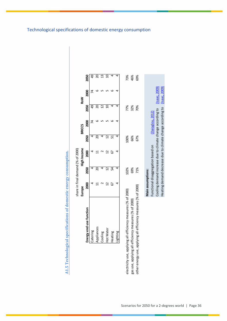
Scenarios for 2050 for a 2-degrees world | Page 36
Technological specifications of domestic energy consumption
A1.5
Tec
hnol
ogic
al s
peci
ficat
ions
of d
omes
tic e
nerg
y co
nsum
ptio
n.
shar
e in
fina
l dem
and
(% o
f 200
0)Eu
rope
High
Inco
me
BRIC
CSRo
WEn
ergy
end
use
func
tion
2000
2050
2000
2050
2000
2050
2000
2050
Cate
ring
44
44
7449
7449
Appl
ianc
es11
2011
206
206
20Co
olin
g2
42
45
125
13Ho
t Wat
er12
1212
125
105
10He
atin
g67
5467
516
46
4Lig
htin
g4
44
44
44
4
elec
tricit
y use
, app
lyin
g all
effic
ienc
y mea
sure
s (%
of 2
000)
102%
100%
77%
73%
gas u
se, a
pply
ing a
ll ef
ficie
ncy m
easu
res (
% o
f 200
0)69
%66
%32
%46
%ot
her e
nerg
y use
, app
lyin
g all
effic
ienc
y mea
sure
s (%
of 2
000)
71%
67%
70%
69%
Mai
n as
sum
ptio
ns:
Func
tiona
l disa
ggre
gatio
n ba
sed
on(D
aiog
lou,
2012
)Co
olin
g dem
and
incr
ease
due
to cl
imat
e ch
ange
acco
rdin
g to
(Isaa
c, 20
09)
Heat
ing d
eman
d de
crea
se d
ue to
clim
ate
chan
ge ac
cord
ing t
o(Is
aac,
2009
)
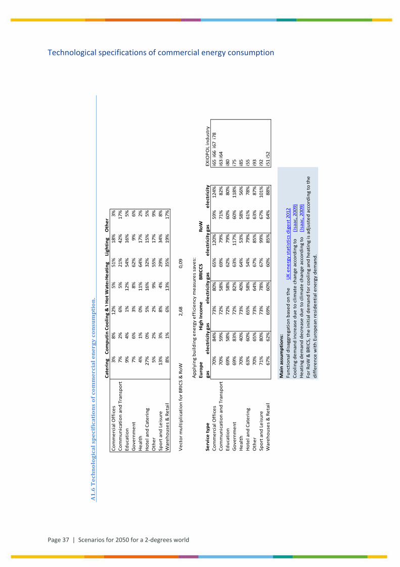
Page 37 | Scenarios for 2050 for a 2-degrees world
Technological specifications of commercial energy consumption
A1.
6 T
echn
olog
ical
spe
cifi
cati
ons
of c
omm
erci
al e
nerg
y co
nsum
ptio
n.
Cate
ring
Com
puti
ngCo
olin
g &
VH
ot W
ater
Hea
ting
Ligh
ting
Oth
erCo
mm
erci
al O
ffic
es3%
8%12
%5%
51%
18%
3%Co
mm
unic
atio
n an
d Tr
ansp
ort
7%2%
6%5%
21%
42%
17%
Educ
atio
n9%
4%1%
12%
54%
16%
5%G
over
nmen
t7%
6%3%
8%62
%9%
6%H
ealt
h4%
1%0%
11%
64%
17%
2%H
otel
and
Cat
erin
g27
%0%
5%16
%32
%15
%5%
Oth
er5%
2%2%
9%55
%17
%9%
Spor
t and
Lei
sure
13%
3%8%
4%29
%34
%8%
War
ehou
ses
& R
etai
l8%
1%6%
13%
35%
19%
17%
Vec
tor m
ulti
plic
atio
n fo
r BRI
CS &
RoW
2,68
0,09
App
lyin
g bu
ildin
g en
ergy
eff
icie
ncy
mea
sure
s sa
ves:
Euro
peH
igh
Inco
me
BRIC
CSRo
WSe
rvic
e ty
pega
sel
ectr
icit
yga
sel
ectr
icit
yga
sel
ectr
icit
yga
sel
ectr
icit
yEX
IOPO
L in
dust
ryCo
mm
erci
al O
ffic
es70
%84
%73
%80
%65
%12
0%59
%12
4%i6
5 i6
6 i6
7 i7
8Co
mm
unic
atio
n an
d Tr
ansp
ort
70%
59%
72%
58%
69%
79%
71%
82%
i63
i64
Ed
ucat
ion
69%
58%
72%
58%
62%
79%
60%
80%
i80
G
over
nmen
t69
%83
%72
%82
%63
%11
7%60
%11
8%i7
5
Hea
lth
70%
40%
73%
40%
64%
53%
58%
56%
i85
H
otel
and
Cat
erin
g63
%60
%65
%58
%54
%79
%61
%78
%i5
5
Oth
er70
%65
%73
%64
%67
%85
%63
%87
%i9
3
Spor
t and
Lei
sure
71%
80%
73%
78%
67%
99%
67%
101%
i92
W
areh
ouse
s &
Ret
ail
67%
62%
69%
60%
60%
85%
64%
88%
i51
i52
Mai
n as
sum
ptio
ns:
Func
tion
al d
isag
greg
atio
n ba
sed
on th
eU
K en
ergy
sta
tist
ics
dige
st 2
012
Cool
ing
dem
and
incr
ease
due
to c
limat
e ch
ange
acc
ordi
ng to
(Isa
ac, 2
009)
Hea
ting
dem
and
decr
ease
due
to c
limat
e ch
ange
acc
ordi
ng to
(Isa
ac, 2
009)
For R
oW &
BRI
CS, t
he in
itia
l dem
and
for c
oolin
g an
d he
atin
g is
adj
uste
d ac
cord
ing
to th
e di
ffer
ence
wit
h Eu
rope
an re
side
ntia
l ene
rgy
dem
and.
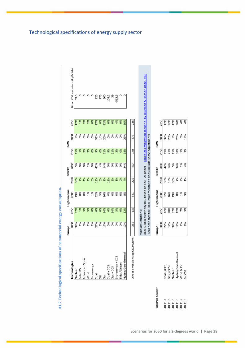
Scenarios for 2050 for a 2-degrees world | Page 38
A1.
7 T
echn
olog
ical
spe
cifi
cati
ons
of c
omm
erci
al e
nerg
y co
nsum
ptio
n.
Euro
peH
igh
Inco
me
BRIC
CSRo
WTe
chno
logi
es20
0020
5020
0020
5020
0020
5020
0020
50D
irec
t CO
2 em
issi
ons
(kg/
MW
h)N
ucle
ar34
%37
%19
%30
%5%
15%
9%17
%59
,5So
lar P
V1%
1%0%
2%0%
1%0%
1%0
Adv
ance
d So
lar
0%3%
0%4%
0%2%
0%2%
0W
ind
1%3%
1%3%
1%2%
0%2%
0Bi
o-en
ergy
1%0%
1%0%
0%0%
0%0%
0Co
al27
%6%
52%
18%
42%
9%32
%17
%82
5O
il7%
0%3%
0%4%
0%14
%0%
775
Gas
17%
14%
16%
9%14
%11
%20
%22
%50
0Co
al +
CCS
0%6%
0%18
%0%
9%0%
0%10
8,2
Gas
+ C
CS0%
14%
0%9%
0%11
%0%
0%39
Bio-
ener
gy +
CCS
0%3%
0%1%
0%3%
0%4%
-512
,5Ti
dal/
Oce
an0%
0%0%
0%0%
0%0%
0%0
Hyd
ro/G
eo-t
herm
al12
%12
%8%
7%34
%38
%25
%36
%0
Dir
ect e
mis
sion
s kg
CO
2/M
Wh
381
136
541
22
5
45
0
14
0
47
6
23
8
Mai
n as
sum
ptio
ns:
2000
& 2
050
elec
tric
ity
mix
bas
ed o
n EM
F-21
pap
er
(mul
ti g
as m
itig
atio
n sc
enar
io, b
y Ja
kem
an &
Fis
cher
, pag
e. 3
40)
Plea
s no
te th
at th
e 20
50 im
plem
enta
tion
doe
s in
clud
e so
me
adju
stm
ents
EXIO
POL
form
atEu
rope
Hig
h In
com
eBR
ICCS
RoW
2000
2050
2000
2050
2000
2050
2000
2050
i40.
11.a
Coal
(+CC
S)27
%12
%52
%36
%42
%19
%32
%17
%i4
0.11
.bG
as(+
CCS)
17%
28%
16%
18%
14%
21%
20%
22%
i40.
11.c
Nuc
lear
34%
37%
19%
30%
5%15
%9%
17%
i40.
11.d
Hyd
ro/G
eo-t
herm
al12
%12
%8%
7%34
%38
%25
%36
%i4
0.11
.eW
ind
& P
V2%
7%1%
9%1%
5%0%
4%i4
0.11
.fBi
oCSS
8%
3%3%
1%4%
3%14
%4%
Technological specifications of energy supply sector

Page 39 | Scenarios for 2050 for a 2-degrees world
Annex B Supply-Use tables
Supply use tables are available at:
http://cml.leiden.edu/research/industrialecology/researchprojects/projects/cecilia/

Scenarios for 2050 for a 2-degrees world | Page 40
Annex C Detailed results
Detailed results inclusive scripts that implement out ‘scenario machine’ are available at:
http://cml.leiden.edu/research/industrialecology/researchprojects/projects/cecilia/
Page 41 | Scenarios for 2050 for a 2-degrees world
Annex D Detailed description of the computational steps per scenario
General approach
For the purpose of CECILIA a scenario that describes a hypothetical economic structure of the world in 2050 including the major carbon emissions has to be made. An environmentally extended input-output model was chosen to implement such a scenario.
Directly adjusting the IO coefficients or making a dynamic closed IO model were rejected as methods to implementing the scenarios. Because EXIOBASE provides supply-use tables, the scenarios could be implemented by manipulating the transactions in the supply-use tables. The manipulated supply-use tables can then in the (environmental) analysis stage be transformed in any type of IO table. Implementing the scenarios in the SUTs has the advantage that the transactions in a supply or use table are more easily interpreted and hence manipulated, the changes as a result of changing transactions (e.g. less volume of electricity use of an industry) can be compensated for in a very specific manner which is more flexible and more transparent and the resulting SUTs can be transformed into different IO tables.
Manipulating transactions in the SUTs means that monetary volume (price times physical flow) is adjusted. In general we will assume that the price remains constant and the change in the monetary transaction is a reflection of the change in the physical flow. The 2050 scenario as implemented in the SUTs will therefore be in 2000 price levels.
Manipulating the supply-use tables has been carried out using a set of Octave scripts2. The basis of the script consists of about 30 smaller functions that carry out a specific task on the supply-use framework. For example checking the balance of the table, calculating efficiency, removing or inserting rows etc. These small functions are all tested in an automated testing procedure. The smaller functions were used to set-up the scripts that implemented one of the scenario assumptions. The main script was a sequence of all these scenario scripts plus some intermediate result logging.
The sequence of scenario steps implemented is as follows:
Step 0: Preprocessing of the initial Supply-Use tables exported from EXIOBASE for the year 2000. The preprocessing step consisted of reading in the tables and getting them fully balanced.
2 GNU Octave is an open source, freely available scripting language which is primarily used for numerical computations. The Octave language is quite similar to Matlab and scripts developed for Octave can be ported to Matlab without too much effort. See http://www.gnu.org/software/octave/
Scenarios for 2050 for a 2-degrees world | Page 42
Step 1: Implementing the foreseen general efficiency improvement in the world economy from 2000 until 2050 and GDP growth. General efficiency change is defined as a reduced use of intermediate use of products by industry while keeping the total output of the industry constant. This general efficiency improvement leads to increased GDP. This GDP growth results in extra income per person. After the efficiency change an extra GDP growth scenario is implemented such that the total GDP growth reflects the foreseen GDP growth in each region from 2000 to 2050. The extra GDP growth can be seen as the growth as a result of population growth while keeping income per person constant. The international trade volumes between the different regions follow GDP growth. The SUTs after step 1 result in the BAU scenario.
Step 2: After the two general economy development scenarios several specific emission reduction technology are implemented in the industry sector and households. The SUTs after step 2 result in the Techno scenario.
Step 1 can be seen as the first step towards the 2050 scenario implementation. The resulting SUTs describe a world in 2050 that has developed along the lines of a business as usual scenario (BAU scenario) without any climate change considerations and continued economic growth. The resulting SUTs after step 1 are therefore interesting to analyze and might be compared to other BAU scenarios such as the IPCC BAU 8.5 scenario (Meinshausen et al., 2011) or OECD baseline scenarios (OECD, 2012a & 2012b).
Step 2 consists of changing the electricity supply mix, several specific technology changes in the electricity supply sectors, and the use of energy in every sector (including final demand). The energy using sectors that are specifically targeted are iron & steel, cement, mobility and energy use in offices and residential buildings.
Below a more detailed description is given of the 2050 scenarios and how they were implemented, with an analysis of the results
Initial supply-use tables from EXIOBASE
The default multi-region supply-use table available in EXIOBASE consists of 43 countries plus one Rest of World region. The supply-use tables of each country/region are divided into 129 industries and 129 products, see Annex E and F for the items distinguished. For the purpose of the CECILIA project multi-region tables were first aggregated to a four region supply-use table. The four regions distinguished are: EU27, high income countries, developing countries and the Rest of World region. The definition of these regions is given in Annex G. The industries and products classification remains at the detailed level of 129 items.
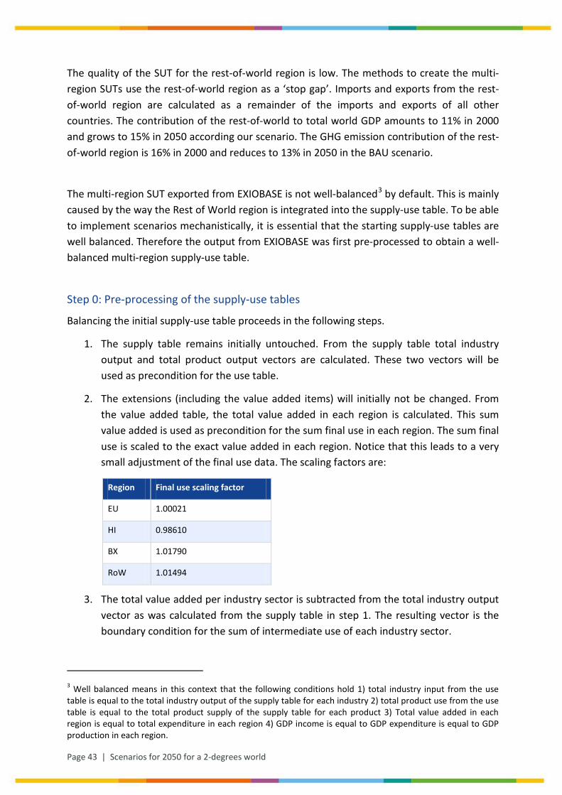
Page 43 | Scenarios for 2050 for a 2-degrees world
The quality of the SUT for the rest-of-world region is low. The methods to create the multi-region SUTs use the rest-of-world region as a ‘stop gap’. Imports and exports from the rest-of-world region are calculated as a remainder of the imports and exports of all other countries. The contribution of the rest-of-world to total world GDP amounts to 11% in 2000 and grows to 15% in 2050 according our scenario. The GHG emission contribution of the rest-of-world region is 16% in 2000 and reduces to 13% in 2050 in the BAU scenario.
The multi-region SUT exported from EXIOBASE is not well-balanced3 by default. This is mainly caused by the way the Rest of World region is integrated into the supply-use table. To be able to implement scenarios mechanistically, it is essential that the starting supply-use tables are well balanced. Therefore the output from EXIOBASE was first pre-processed to obtain a well-balanced multi-region supply-use table.
Step 0: Pre-processing of the supply-use tables
Balancing the initial supply-use table proceeds in the following steps.
1. The supply table remains initially untouched. From the supply table total industry output and total product output vectors are calculated. These two vectors will be used as precondition for the use table.
2. The extensions (including the value added items) will initially not be changed. From the value added table, the total value added in each region is calculated. This sum value added is used as precondition for the sum final use in each region. The sum final use is scaled to the exact value added in each region. Notice that this leads to a very small adjustment of the final use data. The scaling factors are:
Region Final use scaling factor
EU 1.00021
HI 0.98610
BX 1.01790
RoW 1.01494
3. The total value added per industry sector is subtracted from the total industry output vector as was calculated from the supply table in step 1. The resulting vector is the boundary condition for the sum of intermediate use of each industry sector.
3 Well balanced means in this context that the following conditions hold 1) total industry input from the use table is equal to the total industry output of the supply table for each industry 2) total product use from the use table is equal to the total product supply of the supply table for each product 3) Total value added in each region is equal to total expenditure in each region 4) GDP income is equal to GDP expenditure is equal to GDP production in each region.
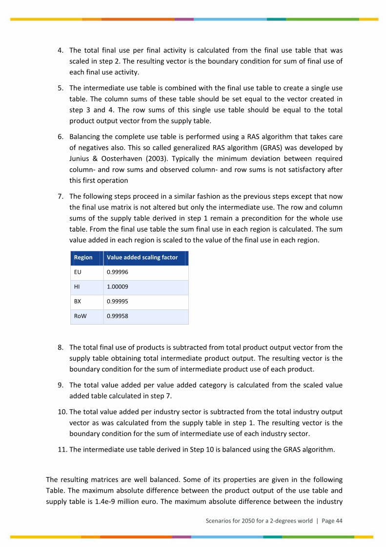
Scenarios for 2050 for a 2-degrees world | Page 44
4. The total final use per final activity is calculated from the final use table that was scaled in step 2. The resulting vector is the boundary condition for sum of final use of each final use activity.
5. The intermediate use table is combined with the final use table to create a single use table. The column sums of these table should be set equal to the vector created in step 3 and 4. The row sums of this single use table should be equal to the total product output vector from the supply table.
6. Balancing the complete use table is performed using a RAS algorithm that takes care of negatives also. This so called generalized RAS algorithm (GRAS) was developed by Junius & Oosterhaven (2003). Typically the minimum deviation between required column- and row sums and observed column- and row sums is not satisfactory after this first operation
7. The following steps proceed in a similar fashion as the previous steps except that now the final use matrix is not altered but only the intermediate use. The row and column sums of the supply table derived in step 1 remain a precondition for the whole use table. From the final use table the sum final use in each region is calculated. The sum value added in each region is scaled to the value of the final use in each region.
Region Value added scaling factor
EU 0.99996
HI 1.00009
BX 0.99995
RoW 0.99958
8. The total final use of products is subtracted from total product output vector from the supply table obtaining total intermediate product output. The resulting vector is the boundary condition for the sum of intermediate product use of each product.
9. The total value added per value added category is calculated from the scaled value added table calculated in step 7.
10. The total value added per industry sector is subtracted from the total industry output vector as was calculated from the supply table in step 1. The resulting vector is the boundary condition for the sum of intermediate use of each industry sector.
11. The intermediate use table derived in Step 10 is balanced using the GRAS algorithm.
The resulting matrices are well balanced. Some of its properties are given in the following Table. The maximum absolute difference between the product output of the use table and supply table is 1.4e-9 million euro. The maximum absolute difference between the industry
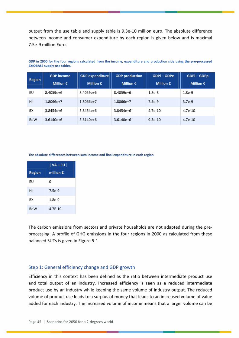
Page 45 | Scenarios for 2050 for a 2-degrees world
output from the use table and supply table is 9.3e-10 million euro. The absolute difference between income and consumer expenditure by each region is given below and is maximal 7.5e-9 million Euro.
GDP in 2000 for the four regions calculated from the income, expenditure and production side using the pre-processed EXIOBASE supply-use tables.
Region GDP income
Million €
GDP expenditure
Million €
GDP production
Million €
GDPi – GDPe
Million €
GDPi – GDPp
Million €
EU 8.4059e+6 8.4059e+6 8.4059e+6 1.8e-8 1.8e-9
HI 1.8066e+7 1.8066e+7 1.8066e+7 7.5e-9 3.7e-9
BX 3.8454e+6 3.8454e+6 3.8454e+6 4.7e-10 4.7e-10
RoW 3.6140e+6 3.6140e+6 3.6140e+6 9.3e-10 4.7e-10
The absolute differences between sum income and final expenditure in each region
Region
| VA – FU |
million €
EU 0
HI 7.5e-9
BX 1.8e-9
RoW 4.7E-10
The carbon emissions from sectors and private households are not adapted during the pre-processing. A profile of GHG emissions in the four regions in 2000 as calculated from these balanced SUTs is given in Figure 5-1.
Step 1: General efficiency change and GDP growth
Efficiency in this context has been defined as the ratio between intermediate product use and total output of an industry. Increased efficiency is seen as a reduced intermediate product use by an industry while keeping the same volume of industry output. The reduced volume of product use leads to a surplus of money that leads to an increased volume of value added for each industry. The increased volume of income means that a larger volume can be
Scenarios for 2050 for a 2-degrees world | Page 46
spent on the final use of products. Hence efficiency change in this context leads to changes in GDP and income per person.
The efficiency change operation has been implemented in an Octave script that adapted the SUTs in the following steps:
1. The general efficiency change coefficient for each industry as described above is applied to its intermediate use of products as recorded in the use table. This leads to a smaller volume of product use while the output of each industry remains the same. This means that there is money generated in each industry that is not spent.
2. This surplus money is transferred to the value added categories of each industry sector proportionally. The change in value added means that there is more money that can be used to buy goods or invest more, i.e. final demand for products should be increased without changing total product supply and keeping the income and final expenditures in each region balanced.
3. This step involves moving the reduced intermediate product use to the final use categories such that total product use still matched total product supply. At this point the SUTs are not balanced because income and final expenditures in each region are not balanced.
4. The system is balanced again following a similar procedure as described in the pre-processing of the initial SUTs resulting in new balanced SUTs.
5. The direct emissions from industries are changed as well. It is assumed that the reduced intermediate use of products (e.g. fuel, fertilizer etc.) brings reduced emissions accordingly. The realized efficiency in each industry sector is calculated and this factor is used to scale down the emissions of CO2, CH4 and N2O emissions. An efficiency increase leads to reduced emissions.
6. The direct emissions from households are adapted as well. Because the efficiency increase leads to increased household consumption we assume that direct emissions from households increase also. The change in private consumption is used as key to change direct emissions from households. The efficiency increase results in direct emissions having a larger contribution to the total emissions in a region.
Following the efficiency change, which leads to GDP growth a further autonomous GDP growth is introduced into the SUTs. GDP change in a region is implemented as an increase of domestic consumption and production in that region. The import and export from the region where GDP is changed follows the GDP change operation. The GDP growth scenario follows the efficiency change scenario. The efficiency change scenario encompassed some GDP growth. The 2000 to 2050 GDP growth scenario is first compared to the GDP growth already
Page 47 | Scenarios for 2050 for a 2-degrees world
accomplished by the efficiency change. The difference is made up for in the GDP growth scenario
GDP change in the multi-region model is implemented mechanistically in the following steps in an Octave script that uses the output of the efficiency change script.
1. The first step when implementing the GDP change is multiplying the complete use table for a particular region with the required GDP change factor. This operation has as side effect that the imports by a region from all other regions is changed as well
2. The value added in each region is multiplied with the appropriate GDP change factor as well.
3. The final use of each product is scaled in the same way as the total intermediate product use.
4. The resulting total industry use and total product use are calculated from the changed intermediate use, final use and value added matrices. These are then forced upon the supply table, adjusting the supply table using the GRAS algorithm.
5. After these first steps the SUTs are not well balanced because the total value added in each region is close but not exactly equal to total final use in a region.
6. Again the supply-use tables are then balanced using the same procedure as used in the pre-processing procedure.
7. The direct emissions from industries are changed as well. It is assumed that the changed intermediate use of products (e.g. fuel, fertilizer etc.) brings changes in emissions accordingly. The changed intermediate product use in each industry sector is calculated and this factor is used to scale the emissions of CO2, CH4 and N2O emissions.
8. The direct emissions from households are adapted as well. Because the GDP growth leads to increased household consumption we assume that direct emissions from households increase also. The change in private consumption is used as key to change direct emissions from households.
The result is new set of well-balanced SUTs that describe the world economy in 2050 which developed along the lines of an economically optimistic business as usual scenario without taking into account any further climate change policy considerations. It is of course a very hypothetical scenario because climate change policy is already affecting the energy use and supply chain and will continue to do so in the future. However this set of SUTs can be used as some sort of baseline/reference scenario in which the specific climate change policy scenarios are implemented which is step 2 of the analysis. The results of step 1 can also be compared with other BAU scenarios such as the IPCC BAU 8.5 scenario.
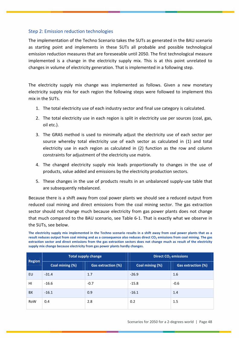
Scenarios for 2050 for a 2-degrees world | Page 48
Step 2: Emission reduction technologies
The implementation of the Techno Scenario takes the SUTs as generated in the BAU scenario as starting point and implements in these SUTs all probable and possible technological emission reduction measures that are foreseeable until 2050. The first technological measure implemented is a change in the electricity supply mix. This is at this point unrelated to changes in volume of electricity generation. That is implemented in a following step.
The electricity supply mix change was implemented as follows. Given a new monetary electricity supply mix for each region the following steps were followed to implement this mix in the SUTs.
1. The total electricity use of each industry sector and final use category is calculated.
2. The total electricity use in each region is split in electricity use per sources (coal, gas, oil etc.).
3. The GRAS method is used to minimally adjust the electricity use of each sector per source whereby total electricity use of each sector as calculated in (1) and total electricity use in each region as calculated in (2) function as the row and column constraints for adjustment of the electricity use matrix.
4. The changed electricity supply mix leads proportionally to changes in the use of products, value added and emissions by the electricity production sectors.
5. These changes in the use of products results in an unbalanced supply-use table that are subsequently rebalanced.
Because there is a shift away from coal power plants we should see a reduced output from reduced coal mining and direct emissions from the coal mining sector. The gas extraction sector should not change much because electricity from gas power plants does not change that much compared to the BAU scenario, see Table 6-1. That is exactly what we observe in the SUTs, see below.
The electricity supply mix implemented in the Techno scenario results in a shift away from coal power plants that as a result reduces output from coal mining and as a consequence also reduces direct CO2 emissions from coal mining. The gas extraction sector and direct emissions from the gas extraction sectors does not change much as result of the electricity supply mix change because electricity from gas power plants hardly changes.
Region Total supply change Direct CO2 emissions
Coal mining (%) Gas extraction (%) Coal mining (%) Gas extraction (%)
EU -31.4 1.7 -26.9 1.6
HI -16.6 -0.7 -15.8 -0.6
BX -16.1 0.9 -16.1 1.4
RoW 0.4 2.8 0.2 1.5
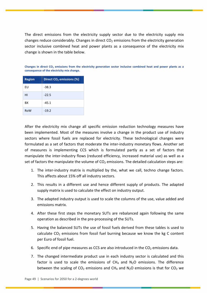
Page 49 | Scenarios for 2050 for a 2-degrees world
The direct emissions from the electricity supply sector due to the electricity supply mix changes reduce considerably. Changes in direct CO2 emissions from the electricity generation sector inclusive combined heat and power plants as a consequence of the electricity mix change is shown in the table below.
Changes in direct CO2 emissions from the electricity generation sector inclusive combined heat and power plants as a consequence of the electricity mix change.
Region Direct CO2 emissions (%)
EU -38.3
HI -22.5
BX -45.1
RoW -19.2
After the electricity mix change all specific emission reduction technology measures have been implemented. Most of the measures involve a change in the product use of industry sectors where fossil fuels are replaced for electricity. These technological changes were formulated as a set of factors that moderate the inter-industry monetary flows. Another set of measures is implementing CCS which is formulated partly as a set of factors that manipulate the inter-industry flows (reduced efficiency, increased material use) as well as a set of factors the manipulate the volume of CO2 emissions. The detailed calculation steps are:
1. The inter-industry matrix is multiplied by the, what we call, techno change factors. This affects about 15% off all industry sectors.
2. This results in a different use and hence different supply of products. The adapted supply matrix is used to calculate the effect on industry output.
3. The adapted industry output is used to scale the columns of the use, value added and emissions matrix.
4. After these first steps the monetary SUTs are rebalanced again following the same operation as described in the pre-processing of the SUTs.
5. Having the balanced SUTs the use of fossil fuels derived from these tables is used to calculate CO2 emissions from fossil fuel burning because we know the kg C content per Euro of fossil fuel.
6. Specific end of pipe measures as CCS are also introduced in the CO2 emissions data.
7. The changed intermediate product use in each industry sector is calculated and this factor is used to scale the emissions of CH4 and N2O emissions. The difference between the scaling of CO2 emissions and CH4 and N2O emissions is that for CO2 we
Scenarios for 2050 for a 2-degrees world | Page 50
look very specifically at fossil fuel use while for CH4 and N2O we use generic product use in each sector as key to scale the CH4 and N2O emissions.
After implementing the technological changes in the industry the generated SUTs are used for the implementation of specific technological changes in the final consumption of products. Also in households there is a shift away from the use of fossil fuels for car driving, household heating towards the use of electricity. The changes in the final consumption were again formulated as a set of consumption change factors.
1. The final demand of products was first multiplied by these consumption change factors.
2. This results in a new total product use as calculated from the row sum of the Intermediate use and final use matrix.
3. This changed total product used to scale the supply matrix resulting in new total industry output values.
4. The changed total industry output calculated from the supply table is subsequently used to scale the columns of the intermediate use table, value added table and emissions matrix.
5. The resulting SUTs are unbalanced and are rebalanced again following the same operation as described in the pre-processing of the SUTs.
6. Having calculated a new final use of fossil fuels the CO2 emissions from fossil fuel burning can be calculated because we know the kg C content per Euro of fossil fuel.
At the end of this operation the resulting SUT reflects the Techno Scenario.
IOT generation
The SUTs generated for each scenario are analysed after they have been transformed into a symmetric product by product – industry technology assumption which is a simple operation and extensively described in Eurostat (2008) or by Konijn (1994).
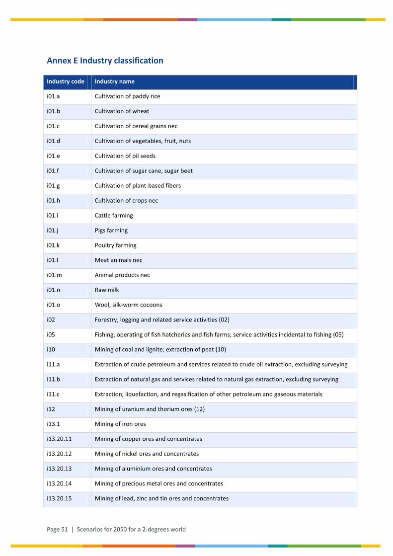
Page 51 | Scenarios for 2050 for a 2-degrees world
Annex E Industry classification
Industry code Industry name
i01.a Cultivation of paddy rice
i01.b Cultivation of wheat
i01.c Cultivation of cereal grains nec
i01.d Cultivation of vegetables, fruit, nuts
i01.e Cultivation of oil seeds
i01.f Cultivation of sugar cane, sugar beet
i01.g Cultivation of plant-based fibers
i01.h Cultivation of crops nec
i01.i Cattle farming
i01.j Pigs farming
i01.k Poultry farming
i01.l Meat animals nec
i01.m Animal products nec
i01.n Raw milk
i01.o Wool, silk-worm cocoons
i02 Forestry, logging and related service activities (02)
i05 Fishing, operating of fish hatcheries and fish farms; service activities incidental to fishing (05)
i10 Mining of coal and lignite; extraction of peat (10)
i11.a Extraction of crude petroleum and services related to crude oil extraction, excluding surveying
i11.b Extraction of natural gas and services related to natural gas extraction, excluding surveying
i11.c Extraction, liquefaction, and regasification of other petroleum and gaseous materials
i12 Mining of uranium and thorium ores (12)
i13.1 Mining of iron ores
i13.20.11 Mining of copper ores and concentrates
i13.20.12 Mining of nickel ores and concentrates
i13.20.13 Mining of aluminium ores and concentrates
i13.20.14 Mining of precious metal ores and concentrates
i13.20.15 Mining of lead, zinc and tin ores and concentrates
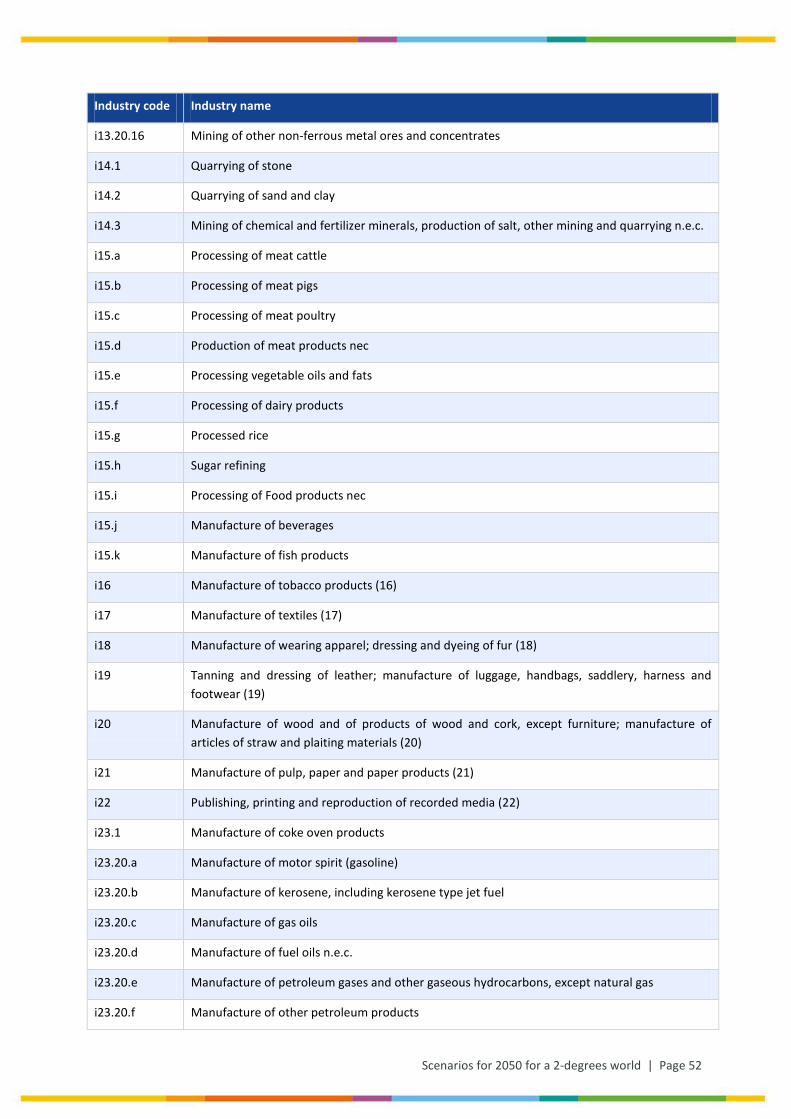
Scenarios for 2050 for a 2-degrees world | Page 52
Industry code Industry name
i13.20.16 Mining of other non-ferrous metal ores and concentrates
i14.1 Quarrying of stone
i14.2 Quarrying of sand and clay
i14.3 Mining of chemical and fertilizer minerals, production of salt, other mining and quarrying n.e.c.
i15.a Processing of meat cattle
i15.b Processing of meat pigs
i15.c Processing of meat poultry
i15.d Production of meat products nec
i15.e Processing vegetable oils and fats
i15.f Processing of dairy products
i15.g Processed rice
i15.h Sugar refining
i15.i Processing of Food products nec
i15.j Manufacture of beverages
i15.k Manufacture of fish products
i16 Manufacture of tobacco products (16)
i17 Manufacture of textiles (17)
i18 Manufacture of wearing apparel; dressing and dyeing of fur (18)
i19 Tanning and dressing of leather; manufacture of luggage, handbags, saddlery, harness and footwear (19)
i20 Manufacture of wood and of products of wood and cork, except furniture; manufacture of articles of straw and plaiting materials (20)
i21 Manufacture of pulp, paper and paper products (21)
i22 Publishing, printing and reproduction of recorded media (22)
i23.1 Manufacture of coke oven products
i23.20.a Manufacture of motor spirit (gasoline)
i23.20.b Manufacture of kerosene, including kerosene type jet fuel
i23.20.c Manufacture of gas oils
i23.20.d Manufacture of fuel oils n.e.c.
i23.20.e Manufacture of petroleum gases and other gaseous hydrocarbons, except natural gas
i23.20.f Manufacture of other petroleum products
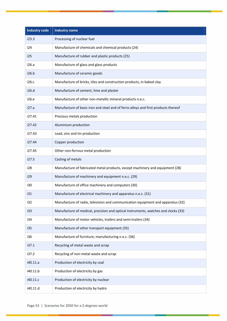
Page 53 | Scenarios for 2050 for a 2-degrees world
Industry code Industry name
i23.3 Processing of nuclear fuel
i24 Manufacture of chemicals and chemical products (24)
i25 Manufacture of rubber and plastic products (25)
i26.a Manufacture of glass and glass products
i26.b Manufacture of ceramic goods
i26.c Manufacture of bricks, tiles and construction products, in baked clay
i26.d Manufacture of cement, lime and plaster
i26.e Manufacture of other non-metallic mineral products n.e.c.
i27.a Manufacture of basic iron and steel and of ferro-alloys and first products thereof
i27.41 Precious metals production
i27.42 Aluminium production
i27.43 Lead, zinc and tin production
i27.44 Copper production
i27.45 Other non-ferrous metal production
i27.5 Casting of metals
i28 Manufacture of fabricated metal products, except machinery and equipment (28)
i29 Manufacture of machinery and equipment n.e.c. (29)
i30 Manufacture of office machinery and computers (30)
i31 Manufacture of electrical machinery and apparatus n.e.c. (31)
i32 Manufacture of radio, television and communication equipment and apparatus (32)
i33 Manufacture of medical, precision and optical instruments, watches and clocks (33)
i34 Manufacture of motor vehicles, trailers and semi-trailers (34)
i35 Manufacture of other transport equipment (35)
i36 Manufacture of furniture; manufacturing n.e.c. (36)
i37.1 Recycling of metal waste and scrap
i37.2 Recycling of non-metal waste and scrap
i40.11.a Production of electricity by coal
i40.11.b Production of electricity by gas
i40.11.c Production of electricity by nuclear
i40.11.d Production of electricity by hydro
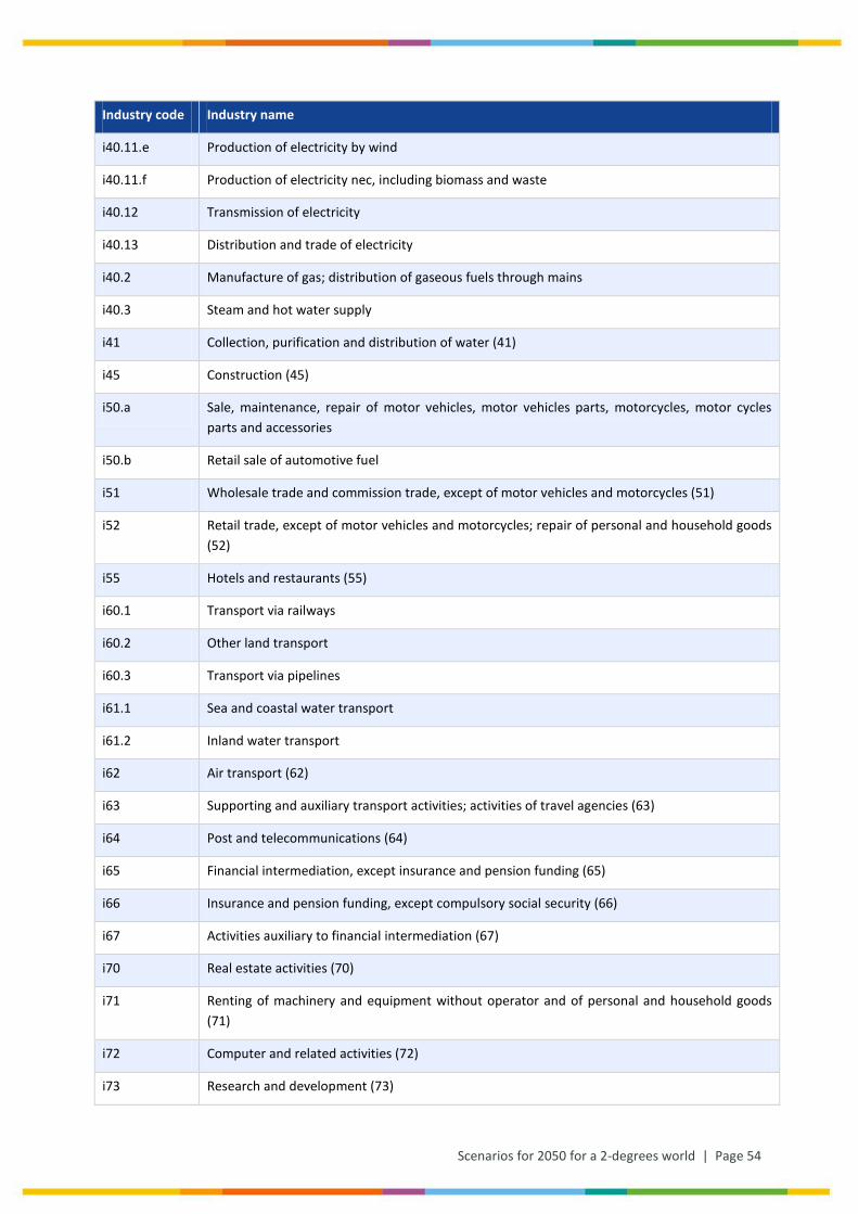
Scenarios for 2050 for a 2-degrees world | Page 54
Industry code Industry name
i40.11.e Production of electricity by wind
i40.11.f Production of electricity nec, including biomass and waste
i40.12 Transmission of electricity
i40.13 Distribution and trade of electricity
i40.2 Manufacture of gas; distribution of gaseous fuels through mains
i40.3 Steam and hot water supply
i41 Collection, purification and distribution of water (41)
i45 Construction (45)
i50.a Sale, maintenance, repair of motor vehicles, motor vehicles parts, motorcycles, motor cycles parts and accessories
i50.b Retail sale of automotive fuel
i51 Wholesale trade and commission trade, except of motor vehicles and motorcycles (51)
i52 Retail trade, except of motor vehicles and motorcycles; repair of personal and household goods (52)
i55 Hotels and restaurants (55)
i60.1 Transport via railways
i60.2 Other land transport
i60.3 Transport via pipelines
i61.1 Sea and coastal water transport
i61.2 Inland water transport
i62 Air transport (62)
i63 Supporting and auxiliary transport activities; activities of travel agencies (63)
i64 Post and telecommunications (64)
i65 Financial intermediation, except insurance and pension funding (65)
i66 Insurance and pension funding, except compulsory social security (66)
i67 Activities auxiliary to financial intermediation (67)
i70 Real estate activities (70)
i71 Renting of machinery and equipment without operator and of personal and household goods (71)
i72 Computer and related activities (72)
i73 Research and development (73)
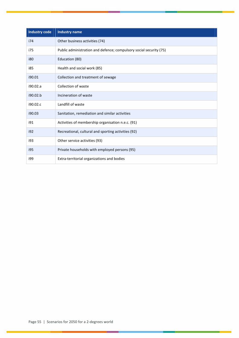
Page 55 | Scenarios for 2050 for a 2-degrees world
Industry code Industry name
i74 Other business activities (74)
i75 Public administration and defence; compulsory social security (75)
i80 Education (80)
i85 Health and social work (85)
i90.01 Collection and treatment of sewage
i90.02.a Collection of waste
i90.02.b Incineration of waste
i90.02.c Landfill of waste
i90.03 Sanitation, remediation and similar activities
i91 Activities of membership organisation n.e.c. (91)
i92 Recreational, cultural and sporting activities (92)
i93 Other service activities (93)
i95 Private households with employed persons (95)
i99 Extra-territorial organizations and bodies
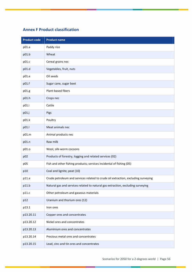
Scenarios for 2050 for a 2-degrees world | Page 56
Annex F Product classification
Product code Product name
p01.a Paddy rice
p01.b Wheat
p01.c Cereal grains nec
p01.d Vegetables, fruit, nuts
p01.e Oil seeds
p01.f Sugar cane, sugar beet
p01.g Plant-based fibers
p01.h Crops nec
p01.i Cattle
p01.j Pigs
p01.k Poultry
p01.l Meat animals nec
p01.m Animal products nec
p01.n Raw milk
p01.o Wool, silk-worm cocoons
p02 Products of forestry, logging and related services (02)
p05 Fish and other fishing products; services incidental of fishing (05)
p10 Coal and lignite; peat (10)
p11.a Crude petroleum and services related to crude oil extraction, excluding surveying
p11.b Natural gas and services related to natural gas extraction, excluding surveying
p11.c Other petroleum and gaseous materials
p12 Uranium and thorium ores (12)
p13.1 Iron ores
p13.20.11 Copper ores and concentrates
p13.20.12 Nickel ores and concentrates
p13.20.13 Aluminium ores and concentrates
p13.20.14 Precious metal ores and concentrates
p13.20.15 Lead, zinc and tin ores and concentrates
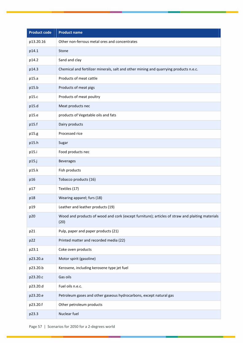
Page 57 | Scenarios for 2050 for a 2-degrees world
Product code Product name
p13.20.16 Other non-ferrous metal ores and concentrates
p14.1 Stone
p14.2 Sand and clay
p14.3 Chemical and fertilizer minerals, salt and other mining and quarrying products n.e.c.
p15.a Products of meat cattle
p15.b Products of meat pigs
p15.c Products of meat poultry
p15.d Meat products nec
p15.e products of Vegetable oils and fats
p15.f Dairy products
p15.g Processed rice
p15.h Sugar
p15.i Food products nec
p15.j Beverages
p15.k Fish products
p16 Tobacco products (16)
p17 Textiles (17)
p18 Wearing apparel; furs (18)
p19 Leather and leather products (19)
p20 Wood and products of wood and cork (except furniture); articles of straw and plaiting materials (20)
p21 Pulp, paper and paper products (21)
p22 Printed matter and recorded media (22)
p23.1 Coke oven products
p23.20.a Motor spirit (gasoline)
p23.20.b Kerosene, including kerosene type jet fuel
p23.20.c Gas oils
p23.20.d Fuel oils n.e.c.
p23.20.e Petroleum gases and other gaseous hydrocarbons, except natural gas
p23.20.f Other petroleum products
p23.3 Nuclear fuel
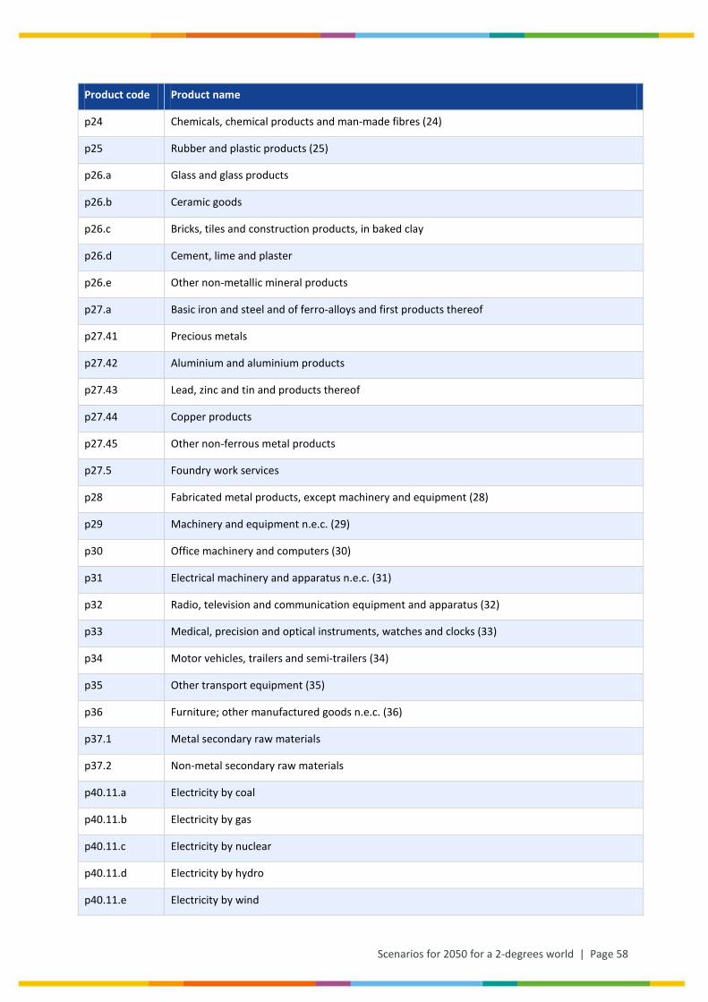
Scenarios for 2050 for a 2-degrees world | Page 58
Product code Product name
p24 Chemicals, chemical products and man-made fibres (24)
p25 Rubber and plastic products (25)
p26.a Glass and glass products
p26.b Ceramic goods
p26.c Bricks, tiles and construction products, in baked clay
p26.d Cement, lime and plaster
p26.e Other non-metallic mineral products
p27.a Basic iron and steel and of ferro-alloys and first products thereof
p27.41 Precious metals
p27.42 Aluminium and aluminium products
p27.43 Lead, zinc and tin and products thereof
p27.44 Copper products
p27.45 Other non-ferrous metal products
p27.5 Foundry work services
p28 Fabricated metal products, except machinery and equipment (28)
p29 Machinery and equipment n.e.c. (29)
p30 Office machinery and computers (30)
p31 Electrical machinery and apparatus n.e.c. (31)
p32 Radio, television and communication equipment and apparatus (32)
p33 Medical, precision and optical instruments, watches and clocks (33)
p34 Motor vehicles, trailers and semi-trailers (34)
p35 Other transport equipment (35)
p36 Furniture; other manufactured goods n.e.c. (36)
p37.1 Metal secondary raw materials
p37.2 Non-metal secondary raw materials
p40.11.a Electricity by coal
p40.11.b Electricity by gas
p40.11.c Electricity by nuclear
p40.11.d Electricity by hydro
p40.11.e Electricity by wind
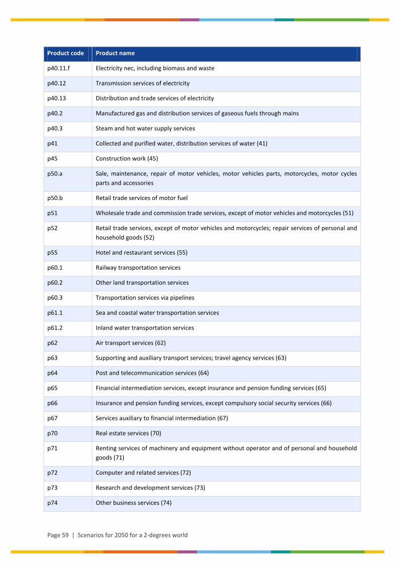
Page 59 | Scenarios for 2050 for a 2-degrees world
Product code Product name
p40.11.f Electricity nec, including biomass and waste
p40.12 Transmission services of electricity
p40.13 Distribution and trade services of electricity
p40.2 Manufactured gas and distribution services of gaseous fuels through mains
p40.3 Steam and hot water supply services
p41 Collected and purified water, distribution services of water (41)
p45 Construction work (45)
p50.a Sale, maintenance, repair of motor vehicles, motor vehicles parts, motorcycles, motor cycles parts and accessories
p50.b Retail trade services of motor fuel
p51 Wholesale trade and commission trade services, except of motor vehicles and motorcycles (51)
p52 Retail trade services, except of motor vehicles and motorcycles; repair services of personal and household goods (52)
p55 Hotel and restaurant services (55)
p60.1 Railway transportation services
p60.2 Other land transportation services
p60.3 Transportation services via pipelines
p61.1 Sea and coastal water transportation services
p61.2 Inland water transportation services
p62 Air transport services (62)
p63 Supporting and auxiliary transport services; travel agency services (63)
p64 Post and telecommunication services (64)
p65 Financial intermediation services, except insurance and pension funding services (65)
p66 Insurance and pension funding services, except compulsory social security services (66)
p67 Services auxiliary to financial intermediation (67)
p70 Real estate services (70)
p71 Renting services of machinery and equipment without operator and of personal and household goods (71)
p72 Computer and related services (72)
p73 Research and development services (73)
p74 Other business services (74)
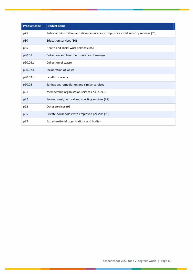
Scenarios for 2050 for a 2-degrees world | Page 60
Product code Product name
p75 Public administration and defence services; compulsory social security services (75)
p80 Education services (80)
p85 Health and social work services (85)
p90.01 Collection and treatment services of sewage
p90.02.a Collection of waste
p90.02.b Incineration of waste
p90.02.c Landfill of waste
p90.03 Sanitation, remediation and similar services
p91 Membership organisation services n.e.c. (91)
p92 Recreational, cultural and sporting services (92)
p93 Other services (93)
p95 Private households with employed persons (95)
p99 Extra-territorial organizations and bodies
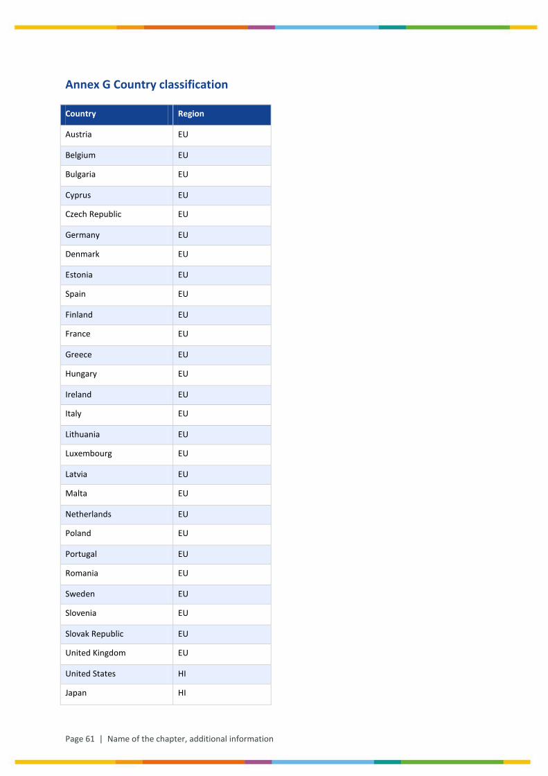
Page 61 | Name of the chapter, additional information
Annex G Country classification
Country Region
Austria EU
Belgium EU
Bulgaria EU
Cyprus EU
Czech Republic EU
Germany EU
Denmark EU
Estonia EU
Spain EU
Finland EU
France EU
Greece EU
Hungary EU
Ireland EU
Italy EU
Lithuania EU
Luxembourg EU
Latvia EU
Malta EU
Netherlands EU
Poland EU
Portugal EU
Romania EU
Sweden EU
Slovenia EU
Slovak Republic EU
United Kingdom EU
United States HI
Japan HI
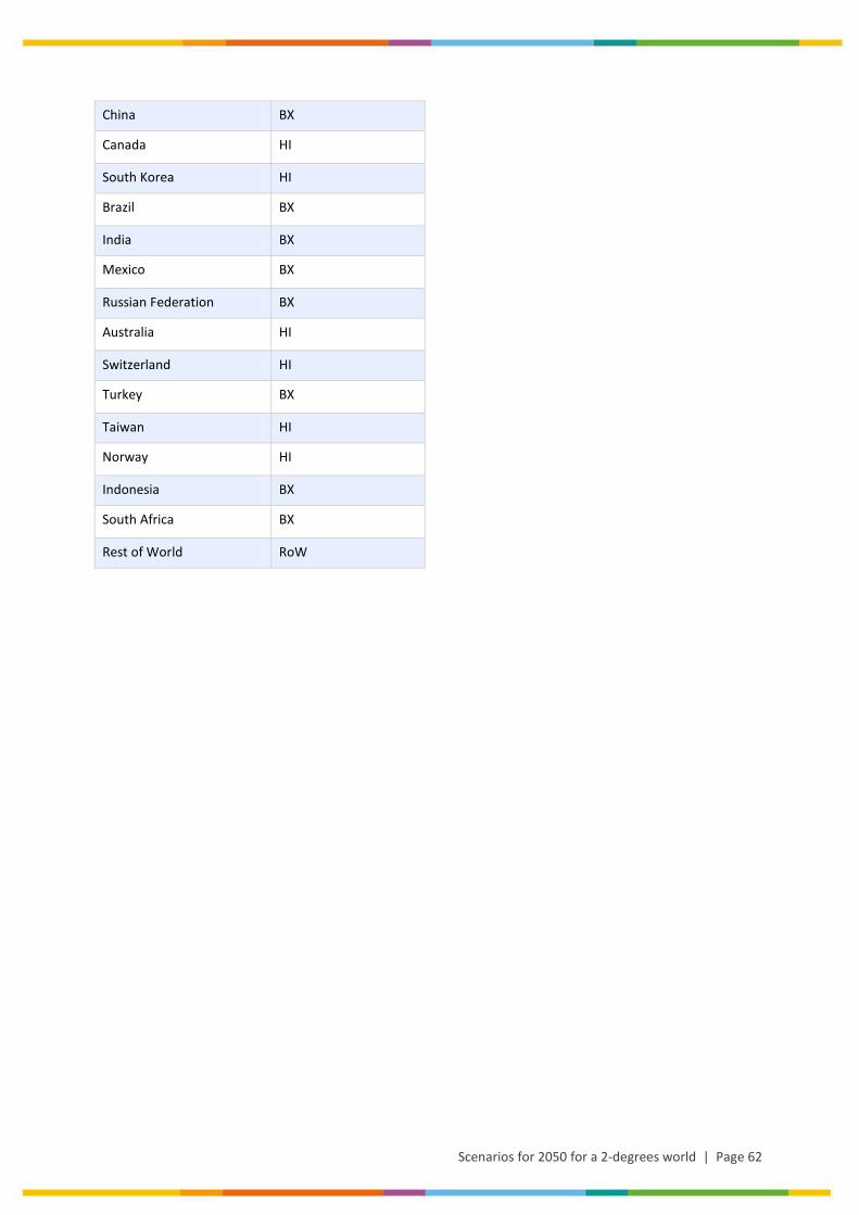
Scenarios for 2050 for a 2-degrees world | Page 62
China BX
Canada HI
South Korea HI
Brazil BX
India BX
Mexico BX
Russian Federation BX
Australia HI
Switzerland HI
Turkey BX
Taiwan HI
Norway HI
Indonesia BX
South Africa BX
Rest of World RoW