Scene Optimized Shadow Mapping

Hamilton. Y. Chong† and Steven J. Gortler‡

Harvard Univeristy

Abstract

Although shadow mapping has found widespread adoption among those who seek realistic and believable lighting,

the algorithm possesses an aliasing issue that is difficult to control. Recent insights have spurred a flurry of

activity and bred a number of novel heuristic approaches to such control. Unfortunately, many of the proffered

heuristics, while improving shadow quality for certain scenes, offer little guarantee outside these specific domains.

In contrast, we present a metric formulation of shadow quality that consequently permits us to solve for optimal

parameters (under a chosen metric) for mitigating the aliasing issue.

Categories and Subject Descriptors (according to ACM CCS): I.3.7 [COMPUTER GRAPHICS]: Three-Dimensional

Graphics and RealismColor, shading, shadowing, and texture

1. Introduction

Although shadow mapping has found widespread adoption

among those who seek realistic and believable lighting, the

algorithm possesses an aliasing issue that is difficult to con-

trol. Recent insights have spurred a flurry of activity and

bred a number of novel heuristic approaches to such control

[SD02, MT04, WSP04]. Unfortunately, many of the prof-

fered heuristics, while improving shadow quality for certain

scenes, offer little guarantee outside these specific domains.

In this work, we generalize the optimization framework in

[Cho03] to handling all 3D scenes. In particular, we present a

metric formulation of shadow quality that consequently per-

mits us to solve for optimal parameters (under a chosen met-

ric) for mitigating the aliasing issue. We do a low resolution

readback of the scene to get an estimate of the geometry and

run an inexpensive optimizer at each frame. For the added

overhead in time, we are able to obtain better shadows using

the same shadow resolution.

Posing shadow map setup as an optimization problem

guarantees a type of robustness to any configuration of lights

and camera. This is in stark contrast to heuristic approaches

that (while perhaps doing no worse than normal shadow

† e-mail: hchong@fas.harvard.edu‡ e-mail:sjg@cs.harvard.edu

mapping) can at times be arbitrarily far from optimal. The

presence of a metric further allows us to quantify the de-

gredation in shadow quality for various shadow map and re-

source choices.

The optimization framework can also notably benefit both

offline and real-time rendering. In offline production set-

tings, shadow maps are often manually tuned with meticu-

lous care. Such work is laborious and not scalable. This re-

search provides a framework for automating this process by

determining optimal shadow map allocations and parame-

ters that guarantee shadow quality within a specified epsilon

tolerance. Real-time applications with constrained configu-

rations can also make use of this as precomputation. Then

during runtime, the metric-based optimization ascertains the

best usage of the allocated resources.

Previous Work. The literature on shadow mapping is

extensive. Since its initial exposition in [Wil78] it has

gained wide adoption and stimulated substantial research.

Filtering [RSC87], hierarchical [FFBG01], light frustum

partitioning [Arv04, Cho03], and shadow volume hybrid

[CD03,CD04,SCH03] methods have been introduced to ad-

dress the aliasing issue. Many of these developments can be

treated orthogonally and incorporated into an optimization

framework. It was only recently observed that shadow map-

ping possesses extra degrees of freedom that can be used to

fight aliasing [SD02,Koz04]. This led to a number of heuris-

tic algorithms [WSP04,MT04] proposing various projective

H. Chong & S. Gortler / Scene Optimized Shadow Mapping

warps to get shadow map sampling to better match the view

camera’s sampling. In [Cho03], the rudiments of an opti-

mization framework is presented, but the work analyzes only

the flatland case. The plane optimal algorithm of [CG04]

is the only attempt at provable shadow quality in 3D, but

only provides guarantees for a few planes of interest. Fur-

thermore, it is shown there exist configurations for which

a single shadow map cannot both obtain perfect sampling

on the specified plane and simultaneously capture the en-

tire shadow frustum of interest, thus requiring division into

smaller sub-frusta. Our work here is closest to [Cho03] in

taking the optimization route. We generalize the setup and

provide solution to this more difficult problem.

2. Method

Notation

~Xl = [X1l ,X2

l ,X3l ,1]t Light space coordinates

~xs = [x1,x2,x3,1]t Screen space coords (position & z)

~u = [u1,u2,u3,1]t Shadow map coords (position & z)

P : ~Xl 7→ wp ·~u Project: light to homogeneous shadow

Q : ~Xl 7→ wq ·~xs Project: light to homogeneous screen

f = PQ−1 :~xs 7→ w f ·~u Maps screen to homogeneous shadow

wp Homogeneous coordinate of P(~Xl)

wq Homogeneous coordinate of Q(~Xl)

w f =wp

wqHomogeneous coordinate of f (~xs)

p̃ti i-th row of matrix P, (i=1,2,3,4)

~q j j-th column of matrix Q−1, ( j=1,2,3,4)

g Metric for size of pixel space footprint

h Functional: shadow quality badness

x1wq

x2wq

x3wq

wq

= Q

X1l

X2l

X3l

1

(1)

The table above introduces the notation used in this paper.

Equation 1 gives an example of what we mean by mapping

into a homogeneous space. We point out that ~xs, ~u, ~Xl , wp,

wq, and w f are all implicitly indexed over a set of geometric

samples. Since each of these quantities shares the same in-

dex, we suppress the index to reduce notational clutter. Par-

ticular attention should also be drawn to the fact that ~q j is

a column of Q−1, not Q itself. It is also worth mentioning

that p̃ti is not the same as the transpose of the i-th column of

P since P is not usually symmetric. The tilde and transpose

symbols are used to emphasize p̃ti is a row vector. In our dis-

cussion we will not be using columns of P or rows of Q−1,

so there should be no confusion in this regard.

2.1. Optimization Framework

Figure 1 shows the relationship between the various domains

of interest. Light space refers to a pre-projective Euclidean

Figure 1: The three domains of interest and the mappings between

them. f can also be interpretted as a mapping from screen to homo-

geneous shadow.

space where the position of the light has been translated to

the origin. Our motivation in using light space instead of

world space as an intermediate domain will become clear

later. Given the view camera’s parameters, the light’s posi-

tion, and a canonical light orientation, the 4x4 matrix Q is

completely determined. The choice of rotation for the light

is unimportant since P has enough freedom to undo any fixed

choice. Our degrees of freedom in shadow mapping then

come from choosing the 4x4 matrix P. We want to choose

P such that each pixel on the screen gets as large a footprint

in the shadow map as possible under the induced mapping

from screen to shadow map. Or to make this a standard min-

imization problem, we seek to minimize the footprint of the

inverse mapping.

We are of course not allowed to choose any 4x4 matrix

for P. We first note that only the first, second, and fourth

rows of P (determining shadow map image coordinates u1

and u2) affect shadow quality (discounting z-buffer preci-

sion issues). Therefore, we ignore the third row of P alto-

gether as something to be optimized separately. By choosing

light space as our intermediate domain, P takes the form of

a camera matrix, mapping the origin (light’s position) to a

point at inifinity with coordinates [0,0,k,0]t for some con-

stant k. The entry k appears in the 3rd row of P which we

threw out. This means that the fourth column of P is already

determined and we are left with only nine entries of P for

optimization. One more degree of freedom is lost to spec-

ifying the overall scale of the projection matrix. One way

to enforce a unique choice of overall scale would be to fix

an element of the matrix to be some constant. As discussed

later, we instead choose to enforce that the fourth row have

unit length. Such a constraint is less convenient for obtaining

analytical solutions, but is conducive to better numerics.

The specific metric for representing footprint size can be

chosen to fit the needs of the application, but any reasonable

metric g will be a function of the derivatives{

dx j

dui

}

. These

provide natural “badness” measures since large values mean

that for unit steps in ui, we move a lot in x j in screen space.

This implies one shadow map sample is referenced by many

H. Chong & S. Gortler / Scene Optimized Shadow Mapping

pixels. We then seek to minimize the integral:

h(P) ≡∫

g

(

dx1

du1,

dx1

du2,

dx2

du1,

dx2

du2

)

I(~xs)dx1dx2 (2)

where I is a weighting function that is zero outside the screen

extents. We note that the dxi/du j are functions of P and ~xs.

Assuming each screen pixel’s shadow quality near shadow

boundaries is equally important, we make I an indicator

function (sum of dirac deltas) for the pixel center samples

near shadow boundaries. This samples the geometry accord-

ing to the screen induced distribution. In our implementation

we choose g to correspond to the L2 norm, so our optimiza-

tion (2) becomes:

minP

h(P) = ∑pixel samples

[

∑i, j=1,2

(

dxi

du j

)2]

(3)

Subject to: 0 ≤ u1 ≤ widthu, ∀screen samples

0 ≤ u2 ≤ heightu, ∀screen samples

|near| < wp ∀screen samples

We note here that the constraints need only be applied to

the convex hull of the points ~Xl as seen on the light’s im-

age plane. Since projective mappings preserve the convex

hull property, enforcing that the convex hull live within the

boundaries of our shadow map texture is enough. The third

constraint is added to ensure that the camera captures all the

points of interest. Violation of this constraint means some

points would be back-projected onto the shadow map image

from behind the camera.

While the Kuhn-Tucker conditions specify the necessary

criteria for achieving a minimization, such nonlinear con-

strained optimization defies general solving [Lue69]. In the

following subsections we take advantage of domain knowl-

edge to present an iterative approach toward an approxi-

mately optimal solution.

2.2. Iterative Solution

As described above, we ignore the third row and fourth col-

umn of P. We solve for the remaining entries of P only up

to scale. The six numbers in the first two rows of P represent

the affine degrees of freedom of the shadow map image. The

leftover three numbers in the fourth row represent the pro-

jective degrees of freedom controlling the optical axis of the

camera. We elimiate the overall scale of the matrix P by con-

straining this fourth row to be unit length. The two remaining

degrees of freedom in p̃t4 can be thought of as controlling the

angling of the film plane at the light [CG04]. Choosing P’s

domain to be light space allows us to interpret, in the most

direct way, the fourth row as exactly specifying the optical

axis of our camera. Aided by this geometric understanding,

the basic algorithm proceeds as listed in Algorithm 1.

In step 1, the color buffer is used to store a bit-mask that

Algorithm 1 OptimizeShadowMap

1. Render scene (shadow receivers) from camera’s view-

point in low resolution → z and bit buffer

2. Read back z-buffer and bit buffer

3. Compute light space pts ~Xl corresponding to camera sam-

ples near shadow boundary

4. Repeat until convergence in h

a. Rotate p̃t4 in negative gradient direction − ∂

∂ p̃t4(h)

b. Approximate optimal affine parameters given p̃t4

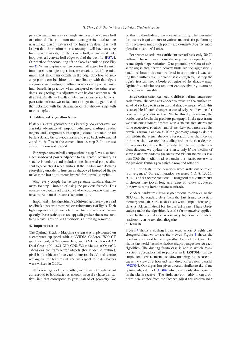
Figure 2: The convex hull (black) is surrounded by the minimum

area rectangle algined with the bottom edge. Since both left and

right extents of non-bottom edge points are to the left of their re-

spective bottom edge extents, we can apply an affine shear to shift

the points right. We then get a better minimum area rectangle fit.

marks which screen pixels are shadowed for each light. The

usual four byte color buffer supports up to 32 such light bit

masks. Shadow maps from the previous frame are used for

shadow determination. While creating and reading back full

sized z-buffers and bit buffers guarantees our shadow maps

are tuned to the needs of each frame, we can do just as well

in most cases by subsampling. We accomplish this by ren-

dering step 1 in low resolution.

In step 3, we use the bit masks to find pixels near

shadow boundaries for each light’s optimization. This im-

proves quality since we optimize only over samples we re-

ally care about. The z-buffer allows us to compute the light

space coordinates of each sample.

Step 4 defines the iterative procedure in which we opti-

mize the projective and affine degrees of freedom in lock-

step. We fix the affine degrees of freedom and optimize the

projective parameters. Then we fix the projective degrees of

freedom and approximately optimize the affine parameters.

− ∂∂ p̃t

4(h) denotes the negative gradient of h with respect to

the variables in P’s fourth row. Since we enforce p̃t4 to be unit

length, we want to update p̃t4 with a rotation instead of the

more usual addition. By keeping only the part of the gradient

vector oriented perpendicular to p̃t4, we get a differential di-

rection in which to rotate the optical axis p̃t4. p̃t

4×(− ∂∂ p̃t

4(h))

defines the axis of rotation. Our problem is now reduced to a

line search. We rotate p̃t4 by various angles ranging between

three and fifty degrees and choose the rotation that gives us

the smallest objective h(P) using the optimal affine parame-

ters.

To compute the affine parameters after rotation, we ob-

serve that our shadow map is rectangular and therefore com-

H. Chong & S. Gortler / Scene Optimized Shadow Mapping

pute the minimum area rectangle enclosing the convex hull

of points ~u. The minimum area rectangle then defines the

near image plane’s extents of the light’s frustum. It is well

known that the minimum area rectangle will have an edge

line up with an edge of the convex hull, so we need only

loop over all convex hull edges to find the best fit [FS75].

Our method for computing affine skew is heuristic (see Fig-

ure 2): When looping over the convex hull edges for the min-

imum area rectangle algorithm, we check to see if the min-

imum and maximum extents in the edge direction of non-

edge points can be shifted to better line up with the edge’s

endpoints. Accounting for affine skew seems to provide min-

imal benefit in practice when compared to the other free-

doms, so ignoring this adjustment can be done without much

ill effect. Finally, to handle shadow maps that do not have as-

pect ratios of one, we make sure to align the longer side of

the rectangle with the dimension of the shadow map with

more samples.

3. Additional Algorithm Notes

If step 1’s extra geometry pass is really too expensive, we

can take advantage of temporal coherency, multiple render

targets, and a fragment subsampling shader to render the bit

buffers during the previous frame and read back subsampled

z and bit buffers in the current frame’s step 2. In our test

cases, this was not needed.

For proper convex hull computation in step 3, we also con-

sider shadowed points adjacent to the screen boundary as

shadow boundaries and include some shadowed points adja-

cent to geometry discontinuities. If the shadow map declares

everything outside its frustum as shadowed instead of lit, we

make these last adjustments instead for lit pixel samples.

Also, every couple frames we generate standard shadow

maps for step 1 instead of using the previous frame’s. This

ensures we capture all disjoint shadow components that may

have moved into the scene after animation.

Importantly, the algorithm’s additional geometry pass and

readback costs are amortized over the number of lights. Each

light requires only an extra bit mask for optimization. Conse-

quently, these techniques are appealing when the scene con-

tains many lights or GPU memory is a limiting resource.

4. Implementation

The Optimal Shadow Mapping system was implemented on

a computer equipped with a NVIDIA GeForce 7800 GT

graphics card, PCI-Express bus, and AMD Athlon 64 X2

Dual Core 4400+ 2.21 GHz CPU. We made use of OpenGL

extensions for framebuffer objects (for render to texture),

pixel buffer objects (for asynchronous readback), and texture

rectangles (for textures of various aspect ratios). Shaders

were written in GLSL.

After reading back the z-buffer, we throw out z values that

correspond to boundaries of objects since they have deriva-

tives in z that correspond to gaps instead of geometry. We

do this by thresholding the acceleration in z. The presented

framework is quite robust to various methods for performing

this exclusion since such points are dominated by the more

plentiful meaningful ones.

For scenes tested it was sufficient to read back only 70x70

buffers. The number of samples required is dependent on

scene depth slope variation. One potential problem of sub-

sampling is that derived convex hulls are too aggressively

small. Although this can be fixed in a principled way us-

ing the z-buffer data, in practice it is enough to just map the

light’s frustum into a bordered region of the shadow map.

Optimality calculations are kept conservative by assuming

the border is unusable.

Since optimization can lead to different affine parameters

each frame, shadows can appear to swim on the surface in-

stead of sticking to it as in normal shadow maps. While this

is accetable if such changes occur slowly, we have so far

done nothing to ensure this. We fix this by increasing the

border described in the previous paragraph. In the next frame

we start our gradient descent with a matrix that shares the

same projective, rotation, and affine skew parameters as the

previous frame’s choice P. If the geometry samples do not

fall within the actual shadow data region plus the increase

in border size, we use the scaling and translation degrees

of freedom to enforce the property. For the rest of the gra-

dient descent, we update our matrix only if the median of

sample shadow badness (as measured via our metric) is less

than 80% the median badness under the matrix preserving

the previous frame’s projective, skew, and rotation.

In all our tests, three iterations were sufficient to reach

“convergence.” For each iteration we tested 3, 5, 8, 15, 23,

30, 40, and 50 degree rotations. The algorithm is quite robust

to choices here too as long as a range of values is covered

(otherwise more iterations are required).

Modern hardware allows asynchronous readbacks, so the

GPU can be sending data from the last frame to system

memory while the CPU busies itself with computations (e.g.,

physics, AI, animation) for the current frame. These obser-

vations make the algorithm feasible for interactive applica-

tions. In the special case where only lights are animating,

readbacks can be avoided altogether.

5. Results

Figure 3 shows a dueling frusta setup where 3 lights cast

elongated shadows toward the viewer. Figure 4 shows the

pixel samples used by our algorithm for each light and also

shows the world from the shadow map’s perspective for each

algorithm. The dueling frusta case is one in which many

heuristic approaches fail to perform well. LiSPSMs, for ex-

ample, tend toward normal shadow mapping in this case be-

cause the view direction and light direction are near parallel

[WSP04]. Our algorithm gives a result similar to the plane

optimal algorithm of [CG04] which cares only about quality

on the planar receiver. The slight sub-optimality in our algo-

rithm here comes from the fact we adjust the shadow map

H. Chong & S. Gortler / Scene Optimized Shadow Mapping

Figure 3: Normal shadow mapping (left). Optimal shadow mapping (center). Plane optimal shadow mapping (right). Each scene is rendered

with 512x512 screen resolution and each light has 256x256 shadow map allocations.

Figure 4: The samples used in optimization (top row). Each algo-

rithm’s shadow map view for the right-most shadow (bottom row).

Light position in shadow maps corresponds to view camera position.

to trade off shadow quality on the dragon as well. Note that

since we find the geometric samples near shadow bound-

aries, our algorithm is able to find a tighter fit about the sam-

ples. If the dragon were not on screen, our algorithm would

compute the same answer as the plane optimal one, but with

a tighter affine fit.

For the numbers presented below, we render a scene with

about 444,000 triangles under 28 “typical” light and cam-

era configurations in 1024x1024 resolution. For comparison

we implement a normal shadow mapping algorithm that in-

cludes a frustum limiting step. This step shrinks the field

of view by projecting the view frustum onto the light frus-

tum’s near plane, intersecting the convex hull of these points

against the light frustum’s near plane extents, and finding a

minimum rectangle about the intersection.

We measure the quality of our shadows by counting the

number of misclassified pixels (shadowed or non-shadowed)

when compared to a truth rendering. The truth rendering is

taken to be one generated with a very high resolution nor-

mal shadow map (3700x3700). The table below gives the

misclassification results for various resolutions. The fourth

column is the percentage more mistakes the normal shadow

mapping algorithm makes over the optimized one.

Number of Misclassified Pixels

Resolution Optimal Normal Percent More

750x750 169360 227202 34.2

1000x1000 128222 176632 37.8

1250x1250 105973 145196 37.0

1500x1500 86943 122780 41.2

1750x1750 77514 106136 36.9

2000x2000 70093 93165 32.9

The following table gives the running time for the two al-

gorithms for different resolution shadow maps and different

number of lights.

Running Time (fps)

# lights Res. Optimal Normal

1 750x750 39.4 59.2

1 1000x1000 38.1 56.9

1 1250x1250 36.4 53.9

1 1500x1500 35.3 50.5

1 1750x1750 34.5 47.2

1 2000x2000 32.6 43.9

2 750x750 28.7 40.0

2 1000x1000 27.7 37.8

2 1250x1250 26.3 35.3

2 1500x1500 24.7 32.7

2 1750x1750 23.6 30.1

2 2000x2000 22.3 27.6

3 750x750 21.4 29.3

3 1000x1000 20.5 27.7

3 1250x1250 19.4 25.7

3 1500x1500 18.4 23.6

3 1750x1750 17.4 21.6

3 2000x2000 16.0 19.7

4 750x750 17.5 23.5

4 1000x1000 16.7 22.1

4 1250x1250 15.7 20.5

4 1500x1500 14.8 18.7

4 1750x1750 13.9 16.9

4 2000x2000 13.0 15.4

H. Chong & S. Gortler / Scene Optimized Shadow Mapping

We see from these tables that as the number of lights

is increased, our algorithm becomes increasingly attractive.

Not only do we get per light memory savings for the same

shadow quality, but the discrepancy in frame rates also

shrinks. For 4 lights, an optimized shadow map with reso-

lution 1250x1250 gives similar quality to a normal shadow

map of resolution 1750x1750 while sacrificing about 1

frame per second (7% of framerate) and saving 6 million

shadow samples.

As an example of the timing profile for scenes in the ex-

periments, a 4 lights and 750x750 shadow map resolution

case is shown in the table below. The optimization timings

include convex hull timings as well. Therefore, the optimiza-

tion time for normal shadow mapping is simply the time it

takes to do convex hull and intersection for limiting the frus-

tum. In optimal shadow maps, the optimization time addi-

tionally includes CPU time spent running the actual opti-

mization procedure. Render & wait includes time for issuing

render calls and waiting for readback or waiting due to throt-

tling from limited GPU pipeline depth.

Time Profile for a 4 light scene using 750x750 shadow maps

Optimal Normal

Time (ms) % total Time (ms) % total

Total scene 56.0 100 41.4 100

Optimization 6.96 12.43 0.16 0.40

Convex Hull 1.10 1.96 0.16 0.40

Render&Wait 49.03 87.57 41.23 99.60

6. Conclusion & Future Work

We have presented an optimization framework for address-

ing shadow map aliasing along with a gradient descent

algorithm for finding solutions. This provides for robust

and quantifiable improvements in shadow quality. Real-

time applications with free texture memory and only a sin-

gle light need not use the method since the cost of read-

back makes any benefit moot. However, as the number of

lights is increased or as texture memory becomes more

tightly constrained, optimal shadow mapping provides in-

creasingly large payoffs. For offline rendering, the cost struc-

ture changes as manual labor must also be factored in as a

resource. More experiments and user studies must be carried

out to evaluate the method’s precise utility in this domain.

References

[Arv04] ARVO J.: Tiled shadow maps. In Proceedings

of Computer Graphics International 2004 (2004), IEEE

Computer Society, pp. 240–247.

[CD03] CHAN E., DURAND F.: Rendering fake soft shad-

ows with smoothies. In Proceedings of the Eurographics

Symposium on Rendering (2003), Eurographics Associa-

tion, pp. 208–218.

[CD04] CHAN E., DURAND F.: An efficient hybrid

shadow rendering algorithm. In Proceedings of the Euro-

graphics Symposium on Rendering (2004), Eurographics

Association, pp. 185–195.

[CG04] CHONG H. Y., GORTLER S. J.: A lixel for every

pixel. In Proceedings of the Eurographics Symposium on

Rendering (2004), Eurographics Association.

[Cho03] CHONG H.: Real-time perspective optimal

shadow maps. Harvard University Senior Thesis (April

2003).

[FFBG01] FERNANDO R., FERNANDEZ S., BALA K.,

GREENBERG D. P.: Adaptive shadow maps. In SIG-

GRAPH ’01: Proceedings of the 28th annual conference

on Computer graphics and interactive techniques (New

York, NY, USA, 2001), ACM Press, pp. 387–390.

[FS75] FREEMAN H., SHAPIRA R.: Determining the

minimum-area encasing rectangle for an arbitrary closed

curve. Commun. ACM 18, 7 (1975), 409–413.

[Koz04] KOZLOV S.: Perspective shadow maps: Care

and feeding. In GPU Gems: Programming Techniques,

Tips, and Tricks for Real-Time Graphics (2004), Addison-

Wesley Professional.

[Lue69] LUENBERGER D. G.: Optimization by Vector

Space Methods. John Wiley and Sons, Inc., 1969.

[MT04] MARTIN T., TAN T.-S.: Anti-aliasing and con-

tinuity with trapezoidal shadow maps. In Proceedings of

the Eurographics Symposium on Rendering (2004), Euro-

graphics Association, pp. 153–160.

[RSC87] REEVES W. T., SALESIN D. H., COOK R. L.:

Rendering antialiased shadows with depth maps. In SIG-

GRAPH ’87: Proceedings of the 14th annual conference

on Computer graphics and interactive techniques (New

York, NY, USA, 1987), ACM Press, pp. 283–291.

[SCH03] SEN P., CAMMARANO M., HANRAHAN P.:

Shadow silhouette maps. ACM Trans. Graph. 22, 3

(2003), 521–526.

[SD02] STAMMINGER M., DRETTAKIS G.: Perspective

shadow maps. In SIGGRAPH ’02: Proceedings of the

29th annual conference on Computer graphics and in-

teractive techniques (New York, NY, USA, 2002), ACM

Press, pp. 557–562.

[Wil78] WILLIAMS L.: Casting curved shadows on

curved surfaces. In SIGGRAPH ’78: Proceedings of the

5th annual conference on Computer graphics and interac-

tive techniques (New York, NY, USA, 1978), ACM Press,

pp. 270–274.

[WSP04] WIMMER M., SCHERZER D., PURGATHOFER

W.: Light space perspective shadow maps. In Proceedings

of the Eurographics Symposium on Rendering (2004), Eu-

rographics Association.

H. Chong & S. Gortler / Scene Optimized Shadow Mapping

Figure 5: Here we show a case with non-planar receivers. In this scene two lights shines down through a skylight with bars. Normal shadow

mapping (left). Scene-optimal (center). World as seen from one of the optimized frusta (right).

Appendix A: Computing Required Quantities

We seek to solve our optimization problem (3) via Algo-

rithm 1. Although we chose the L2 metric for implementa-

tion, what follows is completely general and can be applied

to other metrics. In all cases, we must compute h and its

gradient with respect to p̃t4. To compute h, we require the

derivatives dx j

dui and the rest is straightforwrad. To compute

h’s gradient, we need these same derivatives plus their gra-

dients with respect to p̃t4.

While our interest in computing dx j

dui would suggest it con-

venient to choose as variables the elements of P−1 to avoid

inversion while optimizing the projective degrees of free-

dom, doing so would require an inversion each iteration to

get P for computing the optimal affine parameters. It turns

out to be easier to use the entries of P as our degrees of

freedom, which allows us to conveniently compute dui

dx j . To

perform the computation, we think of x3 as being defined lo-

cally as a function of x1 and x2. We can safely ignore regions

of non-smoothness in x3 as a measure zero set in the [x1,x2]t

domain. By definition we have (for i, j = 1,2):

dui

dx j≡

(

∂ui

∂x j+

∂ui

∂x3

∂x3

∂x j

)

(4)

The ∂x3

∂x j term is computable from the read back z-buffer

values for each pixel and its neighbors. The product rule,

re-arrangement of terms, and factorization into the notated

quantities gives us (for i = 1,2; j = 1,2,3):

∂ui

∂x j=

1

w f

[

∂ (uiw f )

∂x j−ui ∂w f

∂x j

]

∀~xs

=wq

p̃t4~Xl

[

p̃ti~q j −

p̃ti~Xl

p̃t4~Xl

p̃t4~q j

]

∀~Xl (5)

These relations allow us to compute (4).

The inverse function theorem then relates these quantities

to the derivatives we really care about.

[

dx1

du1dx1

du2

dx2

du1dx2

du2

]

=

[

du1

dx1du1

dx2

du2

dx1du2

dx2

]−1

We see that our choice of parameterizing P instead of P−1

yields a 2x2 matrix inversion instead of a 4x4 matrix inver-

sion. To compute h for the L2 metric, we make use of the

explicit formula for the inverse of a 2x2 matrix to obtain:

h

(

dx1

du1,

dx1

du2,

dx2

du1,

dx2

du2

)

= ∑samples

1

(detJ)2

[

∑i, j=1,2

(

dui

dx j

)2]

(6)

where J =

[

du1

dx1du1

dx2

du2

dx1du2

dx2

]

This makes h fully computable from known quantities. To

compute the gradient of h, we apply product rule to Equa-

tion 6. The result is an expression involving derivatives of

the form in Equation 4 and their gradients. So the remaining

ingredient for computing the gradient of h is:

∂

∂ p̃t4

(

∂ui

∂x j

)

=wq

(p̃t4~Xl)2

[(

2(p̃ti~Xl)(p̃t

4~q j)

p̃t4~Xl

− (p̃ti~q j)

)

~Xl − (p̃ti~Xl)~q j

]