Embed Size (px)
Citation preview

Scheduling Alternatives for Mobile WiMAX
End-to-End Simulations and Analysis
by
Carlos Valencia, B.Sc.
A thesis submitted to the Faculty of Graduate Studies and Research
in partial fulfillment of the requirements for the degree of
Master of Applied Science in Technology Innovation Management
Department of System and Computer Engineering,
Carleton University
Ottawa, Canada, K1S 5B6
June, 2009

The undersigned hereby recommend to
the Faculty of Graduate Studies and Research acceptance of the thesis
SCHEDULING ALTERNATIVES FOR MOBILE WIMAX
END TO END SIMULATIONS AND ANALYSIS
Submitted by
Carlos Valencia, B.Sc.
In partial fulfillment of the requirement for the degree of
Master of Applied Science in Technology Innovation Management
Victor Aitken, Department Chair
Thomas Kunz, Thesis Supervisor
Carleton University
June 2009
©Copyright 2009 Carlos Valencia

Abstract
Fourth Generation wireless technologies depend on the performance of their schedulers to
deliver high data throughput and meet quality-of-service commitments. We compare four
schedulers for mobile WiMAX using five industry-defined key performance indicators: sector
and application throughput, completion time, fairness index and delay. The selected scheduling
algorithms are: Proportional Fairness (PF), Modified Largest Weighted Delay First (MLWDF),
Highest Urgency First (HUF), and Weighted Fair Queuing (WFQ). Three simulated
environments are used: controlled, stationary and mobile. The controlled environment provides
insights into the time-related behavior of flows with identical QoS parameters and different RF
conditions. Results for the stationary and mobile environments show that algorithms meet QoS
requirements within system capacity. Opportunistic algorithms (PF and MLWDF) achieve
considerable throughput improvements. MLWDF's throughput results, while better under
stationary conditions, fall behind PF in the mobile scenario. No statistically significant
differences are observed in the mobile environment for application completion time and fairness.

v
Acknowledgements
I greatly acknowledge my thesis supervisor, Professor Thomas Kunz for his competency,
motivation, and eagle's eye to help me produce a sound and high quality thesis. Without his
tireless reviews of my drafts and continuous feedback this document would not have been
possible.
I dedicate this thesis to my beloved family. Thanks to Claudia, my wife, for all her sacrifices
and support during these years, and to Arianna, my three year old daughter, for helping me clear
my mind with her late night visits when mom was already in bed.

vi
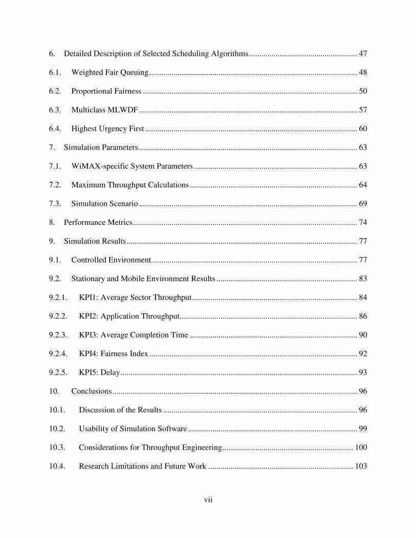
Table of Contents
1. Introduction ............................................................................................................................. 1
1.1. WiMAX Architecture .......................................................................................................... 2
1.2. Thesis Contribution.............................................................................................................. 5
1.3. Thesis Overview .................................................................................................................. 6
1.4. Thesis Structure ................................................................................................................... 7
2. WiMAX Background .............................................................................................................. 9
2.1. Mobile WiMAX PHY........................................................................................................ 11
2.2. Mobile WiMAX MAC....................................................................................................... 13
3. WiMAX Scheduling Techniques........................................................................................... 19
3.1. Algorithms that balance Fairness and Throughput ............................................................ 23
3.2. Algorithms based on Weight/Deficit Calculations ............................................................ 25
3.3. Opportunistic and Cross-Layer Algorithms....................................................................... 27
3.4. Hierarchical / Hybrid Algorithms ...................................................................................... 29
4. Current Options for Mobile WiMAX Simulations................................................................ 32
4.1. Mobile WiMAX Simulation in Qualnet ............................................................................ 33
4.2. Limitations of Qualnet Simulator ...................................................................................... 35
4.3. Qualnet's WiMAX Scheduler ............................................................................................ 37
5. Scheduling Design Dimensions............................................................................................. 40
5.1. Scheduling Subproblems ................................................................................................... 41
5.2. Admission Control and Traffic Shaping ............................................................................ 43
5.3. Meeting QoS while Maximizing Throughput.................................................................... 44
5.4. The Need for Realistic Scenarios....................................................................................... 45
vii
6. Detailed Description of Selected Scheduling Algorithms..................................................... 47
6.1. Weighted Fair Queuing...................................................................................................... 48
6.2. Proportional Fairness ......................................................................................................... 50
6.3. Multiclass MLWDF........................................................................................................... 57
6.4. Highest Urgency First ........................................................................................................ 60
7. Simulation Parameters........................................................................................................... 63
7.1. WiMAX-specific System Parameters ................................................................................ 63
7.2. Maximum Throughput Calculations .................................................................................. 64
7.3. Simulation Scenario ........................................................................................................... 69
8. Performance Metrics.............................................................................................................. 74
9. Simulation Results................................................................................................................. 77
9.1. Controlled Environment..................................................................................................... 77
9.2. Stationary and Mobile Environment Results ..................................................................... 83
9.2.1. KPI1: Average Sector Throughput................................................................................. 84
9.2.2. KPI2: Application Throughput....................................................................................... 86
9.2.3. KPI3: Average Completion Time .................................................................................. 90
9.2.4. KPI4: Fairness Index...................................................................................................... 92
9.2.5. KPI5: Delay.................................................................................................................... 93
10. Conclusions........................................................................................................................ 96
10.1. Discussion of the Results ............................................................................................... 96
10.2. Usability of Simulation Software................................................................................... 99
10.3. Considerations for Throughput Engineering................................................................ 100
10.4. Research Limitations and Future Work ....................................................................... 103

viii
References................................................................................................................................... 106
Appendix A: WFQ Scheduler Class Diagram ............................................................................ 110
Appendix B: CBR and VBR Throughput for Stationary and Mobile Scenarios ........................ 111
Appendix C: Fairness Index Results for Mobile Environment................................................... 114
Appendix D: Delay Results for Mobile Environment ................................................................ 115

ix
List of Figures Figure 1.1-1 WiMAX Architecture.................................................................... 3
Figure 2.1-1 Functional Stages of WiMAX PHY......................................................................... 12
Figure 2.1-2 DL PUSC Permutation............................................................................................. 13
Figure 2.2-1 WiMAX TDD Frame Structure ............................................................................... 14
Figure 2.2-2 WiMAX MAC Layer. Compiled from [7] and [8] .................................................. 15
Figure 3-1 Taxonomy of Scheduling Algorithms for Mobile WiMAX ....................................... 22
Figure 4.3-1 Scheduling a Downlink Subframe ........................................................................... 38
Figure 5.1-1 High Level View of Scheduler................................................................................. 42
Figure 5.3-1 Spectral Efficiency of Different Modulations.......................................................... 45
Figure 6.2-1. Behavior of Ri(t) with tc=80.................................................................................... 51
Figure 6.2-2 Behavior of PF Ratio for tc=80 ................................................................................ 52
Figure 6.2-3 Behavior of Ri(t) for tc=140 ..................................................................................... 52
Figure 6.2-4 Behavior of PF Ratio for tc=140 .............................................................................. 53
Figure 6.2-5 Goodput for Subscribers Under Different Channel Conditions PF tc=100K........... 55
Figure 6.2-6 Goodput for Subscribers Under Different Channel Conditions PF tc=50K............. 56
Figure 6.2-7 Goodput for Subscribers WFQ Scheduler................................................................ 57
Figure 7.3-1 Qualnet Simulation Screenshot ................................................................................ 70
Figure 9.1-1 WFQ Instant Throughput ......................................................................................... 78
Figure 9.1-2 PF Instant Throughput for tc=20000 ........................................................................ 79
Figure 9.1-3 PF Instant Throughput for tc=50000 ........................................................................ 80
Figure 9.1-4 PF Instant Throughput for tc=100000 ...................................................................... 80
Figure 9.1-5 MLWDF Instant Throughput ................................................................................... 82
Figure 9.1-6 HUF Instant Throughput .......................................................................................... 83
Figure 9.2.1-1 Stationary Average Sector Throughput................................................................. 84
Figure 9.2.1-2 Mobile Average Sector Throughput...................................................................... 85
Figure 9.2.2-1 Stationary Application Throughput (FTP only) .................................................... 87
Figure 9.2.2-2 Mobile Application Throughput (FTP Only)........................................................ 88
Figure 9.2.2-3 Stationary Application Throughput (FTP) ............................................................ 89
Figure 9.2.2-4 Mobile Application Throughput (FTP)................................................................. 90
Figure 9.2.3-1 Stationary Average Completion time for FTP ...................................................... 91
Figure 9.2.3-2 Mobile Average Completion Time ....................................................................... 92
Figure 9.2.4-1 Stationary Fairness Index...................................................................................... 93
Figure 9.2.5-1 Stationary Application delay (VoIP)..................................................................... 94
Figure 9.2.5-2 Stationary Application Delay (CBR) .................................................................... 95
Figure 10.3-1 WFQ Throughput Over Time with Flows running at Link Rate ......................... 101
Figure 10.3-2 WFQ Throughput Over Time with Flows Running at MSTR = 1 Mbps............. 102
Figure 10.3-3 PF tc=100K Throughput Over Time with Flows Running at Link Rate .............. 102
Figure 10.3-4 PF tc =100K Throughput Over Time with Flows Running at MSTR = 1 Mbps.. 103

x
List of Tables
Table 2-1 IEEE 802.16 Standards................................................................................................... 9
Table 2-2 WiMAX Forum Mobile System Profile parameters .................................................... 10
Table 2.2-1 WiMAX Scheduling Services ................................................................................... 16
Table 2.2-2 Scheduling Services and their supported QoS Parameters........................................ 17
Table 3.1-1 Algorithms that balance Fairness and Throughput.................................................... 24
Table 3.3-1 Opportunistic Algorithms.......................................................................................... 29
Table 6.1-1 WFQ Behavior........................................................................................................... 49
Table 7.1-1 WiMAX Simulation Parameters................................................................................ 64
Table 7.2-1 Bits per Slot for each Modulation and Coding Scheme ............................................ 65
Table 7.2-2 Calculated Downlink and Uplink Throughput .......................................................... 66
Table 7.2-3 Overhead Calculations IP and MAC Layers ............................................................. 66
Table 7.2-4 Calculated Downlink and Uplink Throughput after Overhead ................................. 68
Table 7.2-5 Measured Single User Downlink and Uplink Throughput........................................ 69
Table 7.3-1 Modulation and Coding Distribution Across Sector ................................................. 71
Table 7.3-2 Application Parameters for Stationary and Mobility Environment Simulations....... 72
Table 10.1-1 KPI Results for Stationary and Mobile Scenarios................................................... 97

xi
List of Acronyms
AMC Adaptive Modulation and Coding
ARQ Automatic Repeat Request
BE Best Effort
BER Bit Error Rate
BS Base Station
CBR Constant Bit Rate
CID
CNS
Connection Identifier
Carrier to Noise Scheduling
DHCP Dynamic Host Configuration Protocol
DRR Deficit Round Robin
DSCP Differentiated Services Code Point
EDF Earliest Deadline First
ertPS extended real-time Polling Service
FEC
FIFO
Forward Error Correction
First In First Out
GPC Grant Per Connection
GPS Generalized Processor Sharing
GPSS Grant Per Subscriber Station
HOL Head Of Line
HUF Highest Urgency First
IEEE Institute of Electrical and Electronic Engineers
MAC Medium Access Control
MAN Metropolitan Area Network
MCS Modulation and Coding Scheme
MIMO Multiple Input Multiple Output
MLWDF Modified Largest Weighted Delay First
MRTR
MS
Minimum Reserved Traffic Rate
Mobile Station
MSTR
NCS
Maximum Sustained Traffic Rate
Normalized CNR Scheduling
nrtPS non real-time Polling Service
OFDM Orthogonal Frequency Division Multiplexing
OFDMa
ORR
Orthogonal Frequency Division Multiple access
Opportunistic Round Robin
PDU Protocol Data Unit
PF Proportional Fair
PHY
PKM
Physical Layer
Public Key Management
QAM Quadrature Amplitude Modulation
QoS Quality of Service
QPSK Quadrature Phase Shift Keying
RLC Radio Link Control

xii
RR Round Robin
RTG Receive Transmit Transition Gap
rtPS real-time Polling Service
SC Single Carrier
SCa Single Carrier access
SDU Service Data Unit
SINR Signal to Interference Noise Ratio
SS Subscriber Station
TDD
TGPS
Time Division Duplex
Truncated Generalized Processor Sharing
TTG Transmit Receive Transition Gap
UGS Unsolicited Grant Service
VoIP
WDRR
Voice over Internet Protocol
Weighted Deficit Round Robin
WFQ Weighted Fair Queuing
WF2Q Worst-case Fair Weighted Fair Queuing
WiMAX Worldwide Interoperability Microwave Access
WirelessHUMAN Wireless High Speed Unlicensed Metro Area Network
WirelessMAN Wireless Metropolitan Area Network
WRR Weighted Round Robin

1
1. Introduction
Despite delays in certification that pushed the delivery of certified MIMO (Multiple In Multiple
Out) products to the end of 2008 [1], and a lot of small to medium size trial deployments yet to
materialize into commercial networks, WiMAX (Worldwide Interoperability Microwave Access)
is still the most immediate solution to provide a mobile broadband wireless solution worldwide.
Its high data rates, quality of service (QoS), mobility, security and scalability features, together
with a healthy industry consortium, are strong reasons for considering it a good alternative for
wireless voice and data services.
IEEE 802.16 standards for Broadband Wireless Metropolitan Area Networks commercially
reflect on two major commercial implementations: Fixed WiMAX, based on 802.16d-2004 [2],
used for stationary deployments and Mobile WiMAX, based on 802.16e-2005 [3], with special
considerations for mobility including handover procedures, added security and a different PHY
layer to support parallel downlink and uplink transmissions. Even though the 802.16e-2005
standard is an amendment to 802.16d-2004, Mobile WiMAX implementations are not backward
compatible with Fixed WiMAX, due mostly to considerable PHY layer differences: Based on
Orthogonal Frequency Division Mulpiplexing (OFDM) for Fixed WiMAX, and on Orthogonal
Frequency Division Multiple Access (OFDMA) based for Mobile WiMAX.
An important component of the WiMAX solution is the scheduler that allocates bandwidth
resources to users on every downlink or uplink transmission. Given the diverse factors that
govern resource allocation in WiMAX (current modulation rate, QoS parameters, and frame
duration) the IEEE committee decided to leave the details of the implementation open. This

2
research work will deal specifically with the issue of efficient scheduling for Mobile WiMAX,
based on the OFDMA PHY layer.
This chapter first presents a general view of the WiMAX architecture, highlighting the scope of
the WiMAX scheduling problem. Contributions of this research are then explained, followed by
a summary of key insights obtained and finally a description of the thesis structure.
1.1. WiMAX Architecture
Figure 1.1-1 presents a simplified view of the WiMAX architecture [4] with emphasis on the
scheduling function provided at the Base Station (BS) entity. The network is IP-based end-to-end
and can be split into three major components: Mobile Stations (MS), also called Subscriber
stations (SS) in the Fixed WiMAX specification; Access Service Network (ASN), which
provides over-the-air connectivity, backhaul services and WiMAX specific features such as
encryption and authentication via the Public Key Management (PKM) module, handover
support, radio resource management and Quality of Service (QoS); and the Connectivity
Services Network (CSN), which is the point of connectivity to the Internet and corporate
networks and provides AAA (Authorization, Authentication and Accounting) services, IP
address assignment, QoS configuration and Mobile IP.
WiMAX has very versatile PHY and MAC layers. While the PHY layer has three distinct
specifications (SC, OFDM and OFDMA), the MAC layer implements several advanced features
such as encryption, security, error correction, link adaptation, power control, automatic
retransmission and quality of service.
The focus of this research is on the interface between MS and BS entities, also called the R1
reference point in WiMAX lingo, which is where the downlink and uplink scheduling takes
place. When a MS connects to the network, a Policy Function residing on the CSN provides the

3
ASN all the classification rules to assign MS' specific traffic to different QoS parameters. Based
on such classification rules, the ASN gateway will set up service flows (one per classification
rule, in each direction) to differentiate the traffic, and can even perform marking of the IP
packets using DSCP (Differentiated Services Code Point) to reflect the different expected
treatment of the packets over the backhaul. These service flows are reflected at the BS entity as
logical connections (called CID, Connection Identifier) to each MS, each one having a specific
scheduling service, according to the defined classification rules.
Air Interface(R1)
Roaming
Interface (R3)IP-based
MS/SS Core Service NetworkAccess Service Network
BS Entity ASN Gw EntityR6
Data Path Data PathEncapsulationEncapsulation
MIP HA
Mobility ManagementHandover Handover Mobility mgmt
Autentication
Authorization
AAA
AutenticationAuthorization
Public Key MgmtPublic Key Mgmt
DL SchedulingIP-based QoS
Policy FunctionQoS configuration
UL SchedulingIP-based QoS
UL trafficClassification
DL traffic DL SchedulingWiMAX QoS
UL SchedulingWiMAX QoS
Figure 1.1-1 WiMAX Architecture
WiMAX brings about a novel concept to wireless systems: Per-flow quality-of-service. A single
subscriber can have different streams of traffic, each one classified and scheduled over the air
based on its quality-of-service parameters. Scheduling decisions get particularly complex as
additional factors are considered:

4
- Different supported modulation and coding schemes (MCS) as well as antenna
techniques such as MIMO Matrix A/B.
- RF conditions might suddenly change, which will change the MCS and hence the amount
of bandwidth that can be allocated on each transmission opportunity.
- Support of error correction methods such as Adaptive Repeat Request (ARQ) and Hybrid
ARQ (H-ARQ).
- PHY multiplexing scheme (OFDM vs. OFDMA).
It is important to highlight that for 802.16e (Mobile WiMAX), the WiMAX Forum™ specifies
OFDMA as the sole PHY mode to be used [5], and contemplates implementation for all of the
MAC features described above. In this context, the MAC scheduling problem for WiMAX
OFDMA can be summarized [6] by three fundamental questions:
1. What criteria should be used to decide the next packet to be scheduled?
2. What modulation shall be used for that specific packet?
3. How should the packets be fit on the OFDMA bi-dimensional frame? Or in more
technical terms “how to construct the complex OFDMA frame matrix as a collection of
rectangles that fit into a single matrix with fixed dimensions?”
In the case of WiMAX OFDM, only questions 1 and 2 require to be answered, while for
WiMAX OFDMA, they must all be answered for every single frame, which can be as often as
every two milliseconds. It is then crucial for the overall network performance to have a
scheduling solution that not only optimizes the costly air link resources but is also efficient and
runs within such demanding constrains.
Extensive research on scheduling solutions for other transmission technologies has been
conducted in the past. Initial scheduler proposals for WiMAX OFDM are based, at least

5
conceptually, on those solutions; however, the application to WiMAX OFDMA cannot be
carried out without additional tweaks and consideration for its more stringent constrains.
The chosen scheduling algorithms were found to be the most relevant available in the literature
for WiMAX OFDM as well as WiMAX OFDMA, answering the three fundamental questions
outlined above as well as presented considerations for supporting multiple QoS scheduling
services.
1.2. Thesis Contribution
In this thesis, emphasis is given to a comprehensive analysis of four scheduling techniques for
downlink traffic in WiMAX. Five industry-defined performance metrics (sector throughput,
application throughput, average completion time, fairness index and delay) are used and their
applicability to the analysis of scheduling techniques in multiple environments (controlled,
stationary and mobility) is explored. Several contributions from this work are presented:
- A review as well as a categorization and analysis of options for WiMAX OFDMA
scheduling currently available in the literature.
- Comparison of recent and promising scheduling proposals under similar conditions. Most
researchers usually propose advanced implementations that are only tested against a well-
known set of scheduling protocols that are not necessarily the most up-to-date options.
While this is important to establish a baseline, a good understanding of the newly
proposed algorithm’s performance compared under similar conditions is preferred.
- Highlight the effects of the characteristics of each environment (controlled, stationary and
mobile) on the defined metrics for each scheduling algorithm and identify alternatives for
better performance and algorithm improvements.

6
1.3. Thesis Overview
This thesis surveys recent techniques proposed to deal with the question of efficient scheduling
of air resources in the WiMAX context, and goes as far as developing the required software to
test three of these techniques in the downlink direction, namely Proportional Fairness (PF),
Modified Largest Weighted Delay First (MLWDF) and Highest Urgency First (HUF), using
Qualnet's WiMAX simulator. The developed algorithms, together with Weighted Fair Queuing
(WFQ, the default scheduling algorithm implemented in Qualnet's software) are analyzed using
five key performance indicators (KPIs: average sector throughput, application throughput,
average completion time and fairness index) defined by the WiMAX Forum, an industry-led
consortium promoting the WiMAX ecosystem.
A scheduler with a good average sector throughput should yield equivalent results in terms of
application throughput, particularly for the FTP Application, which is the only application
simulated in this research that can make use of extra bandwidth if available. Average completion
time and fairness index, both based on the performance of the FTP application, are also
interrelated. A high fairness index (close to 1) would indicate that resources were shared equally
among users with the same bandwidth demands, which would cause, on average, an increase in
completion time. Finally, delay results were obtained for delay sensitive applications (CBR and
VoIP) and verified to ensure that the schedulers did not violate their QoS commitments.
The response of each scheduling algorithm is analyzed first in a controlled environment with no
variation in the radio conditions of each subscriber; second, in a stationary environment by
introducing lognormal shadowing; and third, by adding Rayleigh fading to simulate a pedestrian
environment in an urban setting.

7
The decision to run the simulations under three different environments, even though it increased
the amount of work involved, proved to be highly beneficial as interesting environment-
dependent insights were identified.
For starters, the controlled environment provides an intuitive way to see the behavior of
individual flows over time and the effect scheduling decisions have on them. As a matter of fact
it helped identify a queue leak causing a high amount of dropped packets after running
continuous traffic for a few seconds.
Comparing mobile and stationary environments was equally rewarding. While the stationary
environment results favored PF and MLWDF in terms of throughput and completion time, and
HUF and WFQ in fairness and delay; under mobile environment, three of the defined KPIs
(application throughput, average completion time and fairness index) showed no statistically
significant difference among the analyzed schedulers.
In summary, MLWDF was found to be a comprehensive and customizable algorithm that
maximized throughput while still being able to maintain its QoS commitments. This is in
contrast to PF which, even though it has throughput maximization attributes, does not
incorporate mechanisms to guarantee that QoS is being met.
1.4. Thesis Structure
The thesis is organized as follows. In Chapter 2, background information about WiMAX and its
PHY and MAC layers is presented, with particular emphasis given to the different scheduling
services and their quality of service requirements. Chapter 3 presents previous work in the area
of scheduling algorithms applicable to WiMAX scheduling and provides a taxonomy to
characterize the identified solutions. In Chapter 4, a brief description of Qualnet, the simulation
software chosen for the algorithms' implementation, is presented, including its main features as

8
well as known limitations. Additional insights obtained from the literature review are presented
in Chapter 5, while Chapter 6 provides a detailed description of the four protocols under
analysis. Chapters 7 describes the parameters used for each environment and traffic profiles, and
Chapter 8 describes the performance metrics (also called key performance indicators) used to
analyze each scheduler. Finally, Chapter 9 summarizes all obtained results and Chapter 10
presents conclusions and recommendations.
9
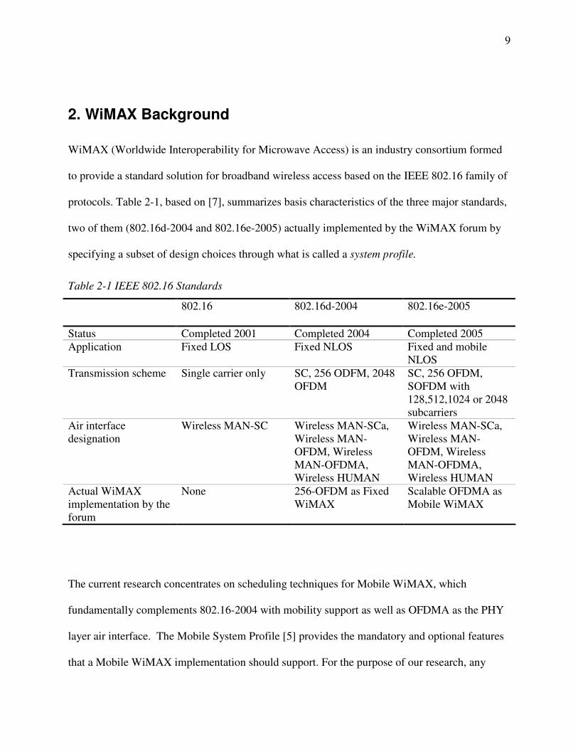
2. WiMAX Background
WiMAX (Worldwide Interoperability for Microwave Access) is an industry consortium formed
to provide a standard solution for broadband wireless access based on the IEEE 802.16 family of
protocols. Table 2-1, based on [7], summarizes basis characteristics of the three major standards,
two of them (802.16d-2004 and 802.16e-2005) actually implemented by the WiMAX forum by
specifying a subset of design choices through what is called a system profile.
Table 2-1 IEEE 802.16 Standards
802.16 802.16d-2004 802.16e-2005
Status Completed 2001 Completed 2004 Completed 2005
Application Fixed LOS Fixed NLOS Fixed and mobile
NLOS
Transmission scheme Single carrier only SC, 256 ODFM, 2048
OFDM
SC, 256 OFDM,
SOFDM with
128,512,1024 or 2048
subcarriers
Air interface
designation
Wireless MAN-SC Wireless MAN-SCa,
Wireless MAN-
OFDM, Wireless
MAN-OFDMA,
Wireless HUMAN
Wireless MAN-SCa,
Wireless MAN-
OFDM, Wireless
MAN-OFDMA,
Wireless HUMAN
Actual WiMAX
implementation by the
forum
None 256-OFDM as Fixed
WiMAX
Scalable OFDMA as
Mobile WiMAX
The current research concentrates on scheduling techniques for Mobile WiMAX, which
fundamentally complements 802.16-2004 with mobility support as well as OFDMA as the PHY
layer air interface. The Mobile System Profile [5] provides the mandatory and optional features
that a Mobile WiMAX implementation should support. For the purpose of our research, any

10
simulation tool chosen should adhere to that profile as much as possible. Some of the parameters
of the system profile important for this research are depicted on Table 2-2. In the next couple of
sections, some of the characteristics of the IEEE 802.16e-2005 PHY and MAC layer are
presented.
Table 2-2 WiMAX Forum Mobile System Profile parameters
Parameter Status Description
PHY Mode Mandatory
OFDMA only
OFDMA is the sole PHY mode defined for mobile
WiMAX
Frame length Only 5ms is
mandatory
Duration of a frame (which corresponds to one downlink
and one uplink subframe) in milliseconds. Several other
frame durations between 2 and 20 ms are allowed
Duplexing
mode
Only TDD
specified
Time division duplexing. BS and MS will use the same
frequency both to transmit and receive.
Subcarrier
allocation
PUSC, FUSC
mandatory for
DL. PUSC and
band AMC
mandatory for UL
Indicates how subchannels (a set of subcarriers, the
minimum frequency domain unit allocated to a user) are
built. They can be constructed using either a contiguous
set of subcarriers (Band AMC) or a set of pseudo-
randomly distributed subcarriers (PUSC and FUSC)
Modulation QPSK,16QAM
and 64QAM
Combined with the coding scheme, will determine how
many bits can be conveyed. 64QAM is optional on uplink
Map support Normal is
mandatory while
submaps are
optional
In order to communicate the allocation of bursts per MS
within the frame a map both for DL and UL is used.
Those maps are modulated QPSK but the submap feature
allows creation of multicast groups that can read submaps
at higher modulations
Convergence
Sublayer (CS)
IPv4 and IPv6
currently
mandatory
What kind of packets can be encapsulated directly within
the WiMAX MAC. Several other CS like Ethernet, ATM,
etc are specified in the standard
Fragmentation Mandatory both
for Tx and Rx
Ability to split a SDU to be transmitted over several
PDUs. On the Rx side, reassembly should be equally
supported.
Data delivery
services
All optional:
UGS, rtVR,
nrtVR, BE and
ertVR
Connection-oriented services conceived to support a
variety of applications. Scheduler must take into account
the requirements of each connection and schedule its
packets accordingly

11
2.1. Mobile WiMAX PHY
Several PHY layers have been defined in IEEE 802.16:
• WirelessMAN SC. Single carrier, aimed at frequencies above 11 GHz with LOS
requirements for point to point operation.
• WirelessMAN SCa. Single carrier, aimed at frequencies between 2 GHz and 11 GHz for
point to multipoint operation.
• WirelessMAN OFDM. The PHY used by Fixed WiMAX, based on 256 FFTs for
operation in non-LOS conditions between 2 GHz and 11 GHz.
• WirelessMAN OFDMA. Initially based on 2048 FFTs for operation in non-LOS
conditions between 2 GHz and 11 GHz. For Mobile WiMAX, this PHY layer has been
extended to support several FFT sizes namely: 128, 512, 1024 and 2048 and it is the sole
PHY layer defined by the WiMAX forum in its Mobile System Profile. OFDMA allows
multiple subscribers to transmit at the same time during a frame.
• WirelessHUMAN. Similar to the MAN OFDM specification, with the exception that it
focuses on unlicensed bands.
Figure 2.1-1 [7] provides an overview of the several functional stages that compose the PHY
layer including:
• Forward Error Correction (FEC) including channel encoding, rate matching, interleaving
and symbol mapping. Steps to support PHY layer retransmissions (H-ARQ) are also
performed at this stage.
• Construction of the OFDM symbol in the frequency domain including space/time coding
or MIMO if available, inserting pilot subcarriers for channel estimation purposes and
performing subcarrier allocation. The subcarrier allocation process corresponds to the

12
mapping of subcarriers into subchannels using a subcarrier permutation scheme (PUSC,
FUSC, and Band AMC). Those subchannels will later be allocated to specific slots,
which is the basic PHY layer allocation unit for a user.
• Conversion of the OFDM symbol from the frequency domain to the time domain through
a series of Inverse Fast Fourier Transforms (IFFT) and eventually into the analog domain.
Figure 2.1-1 Functional Stages of WiMAX PHY
Figure 2.1-2[7] shows how the subcarrier allocation is performed in the case of the DL PUSC
permutation scheme. Other permutation schemes operate in a similar fashion. Fourteen
consecutive subcarriers over two symbols are arranged into clusters, which are then renumbered
using a pseudorandom scheme and assigned to one of six groups. Two clusters from the same
group will then form a subchannel. This subchannel is the frequency domain allocation that will
compose a slot. In the case of DL PUSC, a slot is one subchannel (composed of 24 subcarriers)
by two OFDM symbols.

13
Figure 2.1-2 DL PUSC Permutation
2.2. Mobile WiMAX MAC
Figure 2.2-1 shows a WiMAX TDD frame structure. Both downlink and uplink subframes are bi-
dimensional structures composed of subchannels over a certain number of symbols. Each burst is
assigned to a particular user and it is composed of an integer number of slots.
It is up to the MAC layer to allocate these slots to specific subscribers based on their QoS
requirements and network conditions. Depending on their throughput requirements and resource
availability, a subscriber can be assigned as little as a single slot or as many as all the available
slots within the corresponding subframe. Slot allocation information is contained either in the
downlink or uplink map depending on the direction of the connection.

14
P
r
e
a
m
b
l
e
sub
ch
ann
el Lo
gic
al n
um
be
r
1
N
F
CH
OFDM Symbol Number
DL
Ma
p
UL
Ma
p
0 N-1
U
L
M
ap
DL Burst #2
Coded symbol write order
DL Burst #4
DL Burst #3
DL Burst #5
DL Burst #7
DL Burst
#6
DL subframe UL subframe
DL Burst
#1
0 M-1
ACK
Ranging
Fast Feedback
Burst 1
Burst 2
Burst 3
Burst 4
Burst 5
Guard
Figure 2.2-1 WiMAX TDD Frame Structure
Figure 2.2-2 shows the main components of the WiMAX MAC and how data gets converted
from packets all the way to bursts that will be transmitted by the PHY layer on a subframe. Some
critical functions of the MAC are:
• Segment or concatenate service data units (SDUs) received from upper layers into MAC
protocol data units (PDUs).
• Select the appropriate modulation and coding as well as the power level for the
transmission of each burst.
• Retransmission of errored PDUs if ARQ is being used.
• Provide security and key management.

15
• Provide support to mobility functions.
• Provide QoS control and priority handling of MAC PDUs.
• Schedule MAC PDUs over the PHY resources. In the downlink direction, all scheduling
decisions are made at the BS as packets arrive into different scheduling services. In the
uplink direction, MS can be granted periodic opportunities to transmit or should send
requests for bandwidth, which will be scheduled by the BS entity and indicated to the MS
in a subsequent UL map. The following section will explain this process in more detail.
Higher layer
MAC Convergence Sublayer
(header suppression and SFID and CID identification)
MAC Common Part Sublayer
(assembly MAC PDUs, ARQ scheduling, MAC management)
MAC Security Sublayer (encryption)
PHY
DataManagement
signalling
Traffic Data
MAC SDU
ARQ BlockMSDU Fragment
Non-ARQtraffic
ARQtraffic
DL Burst #2
DL Burst #4
DL Burst #3
DL Burst #5
DL Burst #7
DLBurst
#6
DLBurst
#1
PayloadMAC
headerSub
header
MAC
PDU
MAC
PDU...
MAC
PDU
MAC
PDU
PayloadMAC
headerSub
header
DL Burst #2 DL Burst #4
Figure 2.2-2 WiMAX MAC Layer. Compiled from [7] and [8]
16
WiMAX owes its QoS versatility to the different scheduling services supported, which determine
how the network will allocate UL and DL transmission opportunities as well as how the MS can
request uplink resources. The five scheduling services defined in the standard are shown on
Table 2.2-1. A scheduler designed for WiMAX should take into account and accommodate the
requirements of each scheduling service.
Table 2.2-1 WiMAX Scheduling Services
Scheduling
Service
Application Access to resources
Unsolicited
Grant
Service
(UGS)
Real time service flows of
constant bit rate and low jitter
and delay tolerance such as
circuit emulation or VoIP.
Fixed periodic amount of BW is assigned to
the connection; MS cannot request additional
UGS BW but can request replacement of lost
BW via a Slip Indicator (SI). A Poll Me (PM)
bit can be used to request a unicast poll for BW
needs on non-UGS connections.
real time
Polling
Service
(rtPS)
Real time service flows of
variable data rate such as
streaming video
Periodic request opportunities are assigned,
which allow an MS to specify the amount of
BW required each time. MS cannot use
contention requests opportunities, only the
assigned unicast poll.
Non-real
time Polling
Service
(nrtPS)
Can be used for TCP-based
applications with relaxed delay
sensitivity such as FTP.
Similar to rtPS but polling period is longer and
contention request opportunities are allowed
even though they can be restricted via the
transmission/request policy
Best Effort
(BE)
For services that do not have
any QoS requirements, HTTP
or e-mail for example
All forms of polling are allowed
Extended
real time
Polling
Service
(ertPS)
Real time services for which the
bit rate varies slightly in time.
Implemented having VoIP with
silence suppression in mind
MS is allowed to change its BW requirements
over time. Periodic grants are assigned like in
UGS, those grants can be used to transmit data
as well as for requesting additional BW (unlike
UGS).
Some applications such as voice over IP will have very stringent delay and jitter constrains,
while consuming little bandwidth; others, such as video streaming, will require much more
bandwidth, but are more resilient to longer delays. The quality of service requirements of a
certain application, like the maximum tolerated latency and jitter and the minimum throughput

17
required to operate properly are mapped into QoS parameters and depending on these
parameters, mapped to a scheduling service that supports them. Table 2.2-2 shows the scheduling
services and QoS parameters supported by each one. Applications should be mapped to a
scheduling service that supports the QoS parameters that they require to operate properly. Voice
over IP for example, which requires a consistent delay and jitter should be mapped to UGS or
ertPS (ertPS having the advantage that bandwidth requirements can change over time, so during
silence periods the bandwidth requirement can be set to zero), while an e-mail application, which
does not have an specific bandwidth or delay requirement can be sent over a BE scheduling
service.
Table 2.2-2 Scheduling Services and their supported QoS Parameters
QoS parameter UGS rtPS nrtPS BE ertPS
Maximum Sustained Traffic Rate (MSTR).
Defines the peak information rate (bits per
second) of the service. Used for policing and
traffic shaping of the flow
Y Y Y Y Y
Minimum reserved traffic rate (MRTR).
Specifies the minimum rate (bits per second)
reserved for the flow calculated excluding
MAC overhead
N Y Y N Y
Maximum latency. Specifies the maximum
interval between the reception of the packet
at the transmit end and the arrival of the
packet at the receive end
Y Y N N Y
Tolerated jitter. Specifies the maximum
delay variation for the connection.
Y N N N Y
Traffic priority. Specifies the priority of the
associated service flow. It is used to
prioritize one flow over the other
N Y Y Y Y
When a WiMAX subscriber ranges into the network, two bi-directional MAC layer connection
identifiers (CID) are set up for management traffic between the subscriber and the BS entity: A

18
primary CID, which is used for delay-sensitive management messages such as ranging or
bandwidth allocation; and a basic CID, used for less sensitive MAC messages such as IP address
request. Additionally, unidirectional data CIDs will be set up to identify specific traffic flows
between the subscriber and the BS. It is these data CIDs that could map into different scheduling
services depending on classification rules defined for the user.
For the downlink, it is up to the BS entity to decide which packets to schedule next as queues for
different scheduling services start to fill up. It will then communicate the scheduling decision in
the DL map, together with the corresponding burst within the same frame.
In the uplink direction the process is a little more complex. Depending on the scheduling service,
connections can either have periodic transmission grants (UGS, ertPS), periodic opportunities to
request BW (ertPS, rtPS, nrtPS), or contention opportunities to request BW (ertPS,nrtPS, BE).
These grants can then be allocated based on two modes:
• GPSS: Grant per subscriber station. BS grants bandwidth based on the aggregate of
requests. Grant is communicated to the SS (Subscriber Station) via its primary CID
(Connection Identifier). It is then up to the subscriber to decide how to distribute the BW,
and the SS itself has to apply a certain level of scheduling logic to decide what
connection to allocate the grant to.
• GPC: Grant per connection. The BS Entity decides the specific connection to grant the
bandwidth to. As this mode is more controlled and saves scheduling decisions at the
subscriber, it introduces additional overhead as now the UL map should have grant
information for each connection.
GPSS will be most likely the mode of choice as it allows for higher scalability since it saves a
considerable amount of space on the UL map.

19
3. WiMAX Scheduling Techniques
Queuing theory as well as scheduling techniques are widely researched topics in
telecommunications and computing. It is reasonable then that initial scheduler solutions for
WiMAX were adaptations of current scheduling techniques already proven for other
technologies. Additionally, over the last few years there has been a good amount of research on
complementary techniques to take into account the variability of the wireless channel through
opportunistic algorithms, channel awareness and cross-layer designs.
While some similarities to the wired world can be drawn, there are certain characteristics of the
wireless environment that make scheduling particularly challenging. Five major issues in
wireless scheduling are identified in [9] :
• Wireless link variability: Due to characteristics of the channel as well as location of the
mobile subscribers.
• Fairness: Refers to optimizing the channel capacity by giving preference to spectrally
efficient modulations while still allowing transmissions with more robust modulations
(and hence, consuming a major amount of spectrum) to get their traffic through.
• QoS: Particularly for WiMAX, QoS support should be built into the scheduling algorithm
to guarantee that QoS commitments are meet under normal conditions as well as under
network degradation scenarios.
• Data throughput and channel utilization: Refers to optimizing the channel utilization
while at the same time avoiding waste of bandwidth by transmitting over high loss links.

20
• Power constrain and simplicity: Be considerate of the terminals’ battery capacity as well
as computational limitations both at the BS and MS.
Figure 3-1 presents a taxonomy of scheduling algorithms found in the literature. Even though
there is no clean cut between each branch, it helps to visualize some of the techniques used and
to explain the basic concepts behind them.
Early algorithms have characteristics that clearly differentiate them and hence are easily
classified; [7] and [10], for example, define algorithms in terms of what gets optimized:
maximum overall capacity, fairness in terms of allocating resources equally to all the users, or
fairness proportional to bandwidth requirements or link condition. More recent algorithms are
much harder to categorize as they usually combine several techniques targeting specific
requirements of each scheduling service in order to meet QoS requirements, while implementing
some sort of fairness to avoid starvation of BE and nrtPS connections and even incorporate
admission control.
While we adopt part of the taxonomy proposed by [11], algorithms are matched to their
respective families based on similarities in their formulation as well as the parameters used to
make the scheduling decision:
• Balance fairness and throughput. Algorithms that pursue a middle ground between sector
throughput and allocating a fair amount of resources to subscribers in the sector share the
basic formulation presented in [12]. Proportional Fairness is a representative example of
this category.
• Based on weight/deficit calculations. This category includes algorithms implementing
calculations assigning weights, deficit, or delay counters to each connection that later will

21
be used to perform scheduling decisions. Solutions inspired by general processor sharing
algorithms like TGPS, WRR and DRR are representative examples of this category.
• Opportunistic and cross-layer algorithms. Opportunistic algorithms look at exploiting the
variability of the wireless channel condition by giving preference of transmission to
subscribers with good channel quality [13]. The term “cross-layer algorithm” is used
extensively and requires extra care; [14] presents a taxonomy identifying six different
kinds of cross-layer designs. In the context of this research, cross-layer refers to
algorithms that integrate both the scheduling of packets to meet QoS commitments and
the scheduling of radio link resources (slots, subchannels) to optimize them. MLWDF,
for example, factors in a QoS-based priority and a delay counter, as well as channel
capacity information in its scheduling decision.
• Hierarchical and hybrid algorithms are algorithms that combine several scheduling
techniques, in order to meet the particular needs of each scheduling class. Usually these
algorithms distribute the available resources among the different scheduling services, as
the first layer of the hierarchy, and then independent scheduling techniques are applied to
decide the next packet to be scheduled for each scheduling service. Some solutions also
incorporate a certain level of admission control to avoid starvation of lower priority
scheduling services.

22
Balance fairness and
throughput
Based on weight/
deficit calculations
Opportunistic and
crosslayer
Scheduling algorithms for
Mobile Wimax
Proportional Fairness
=1, =1
PF with data rate
control
is a fixed value for
all SS
Adaptative PF
is a calculated
value for all SS
Round robin
Max SNR
=1, =0TGPS
WRR
DRR
WFQCNS or
MAx MCS
Hybrid
Hierarchical
EDF
WDRR
Hierarchical with EXP
rule for rtPS/nrtPS
MLWDF &
multiclass MLWDF
HUF
NCS
ORR
EDF + WFQ+FIFO
EDF + WFQ
Figure 3-1 Taxonomy of Scheduling Algorithms for Mobile WiMAX
23
A classification of recent scheduling proposals for WiMAX is also presented in [15], where
scheduling techniques are classified in two main categories: channel-unaware and channel aware
depending on whether or not RF channel information is used for scheduling decision. Channel-
aware algorithms are further categorized based on the objective of their formulation: fairness,
QoS guarantee, system throughput maximization and power optimization.
While this classification is interesting, we believe a taxonomy based on formulation and method
of operation helps identify better commonalities among schedulers. For example, according to
the channel-unaware vs. channel-aware classification, WFQ would be a channel-unaware
algorithm, but that same algorithm could be adapted to make it channel-aware by incorporating
dynamic channel conditions into the calculation of a connection's weight.
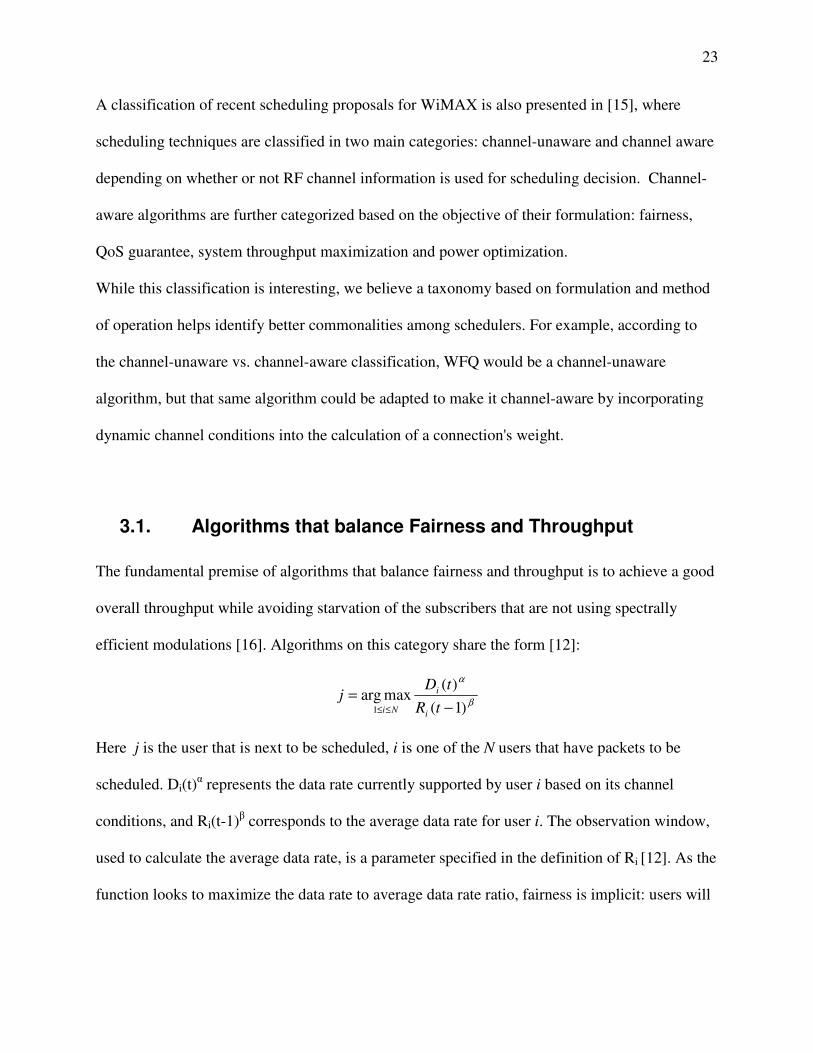
3.1. Algorithms that balance Fairness and Throughput
The fundamental premise of algorithms that balance fairness and throughput is to achieve a good
overall throughput while avoiding starvation of the subscribers that are not using spectrally
efficient modulations [16]. Algorithms on this category share the form [12]:
β
α
)1(
)(maxarg
1 −=
≤≤ tR
tDj
i
i
Ni
Here j is the user that is next to be scheduled, i is one of the N users that have packets to be
scheduled. Di(t)α represents the data rate currently supported by user i based on its channel
conditions, and Ri(t-1)β corresponds to the average data rate for user i. The observation window,
used to calculate the average data rate, is a parameter specified in the definition of Ri [12]. As the
function looks to maximize the data rate to average data rate ratio, fairness is implicit: users will

24
be scheduled if they can support a good data rate Di(t)α , but users that start to average a low data
rate will eventually get scheduled.
The parameters α and β are tuning parameters. α can be used as a method to limit the data rate,
and hence incorporate traffic shaping into the algorithm. β can be factored in to control the way
the data rate averaging is performed. Table 3.1-1 shows different combinations of α and β found
in the literature.
Even though these algorithms perform reasonably well at balancing throughput vs. fairness over
the air link, one can conclude by looking at the formulation that prioritization is not embedded in
the algorithm itself. Additional steps need to be taken to incorporate prioritization among
scheduling services. In [17] for example, a simple method is used to deal with this situation: the
minimum number of slots to meet QoS requirements are pre-allocated in order: UGS first, rtPS
second and only then unused slots are allocated to other scheduling services in order : nrtPS and
BE; ertPS is not considered here.
Table 3.1-1 Algorithms that balance Fairness and Throughput
Α Β Algorithm
1 1 PF algorithm used in CDMA EVDO 1x [16]. It is the prime example of this
category as it uses the feedback on the currently used MCS, combined with the
average data rate used by each subscriber to determine which packet gets
access to the resources.
1 0 Max SNR [10] algorithm, which always serves the terminal with best RF
conditions. Although it optimizes overall throughput, it doesn’t have any
fairness considerations.
0 1 Round robin [11] scheduling with time slots assigned according to the average
data rate of each subscriber
n 1 PF with data rate control [12]. n is a predetermined value that will control the
data rate allocated to subscribers. The value of n is the same for all subscribers
and hence different data rate limits cannot be allocated
Ci 1 Adaptive PF [12] . It complements the previous algorithm by introducing Ci, a
dynamic data rate control value for user i
25
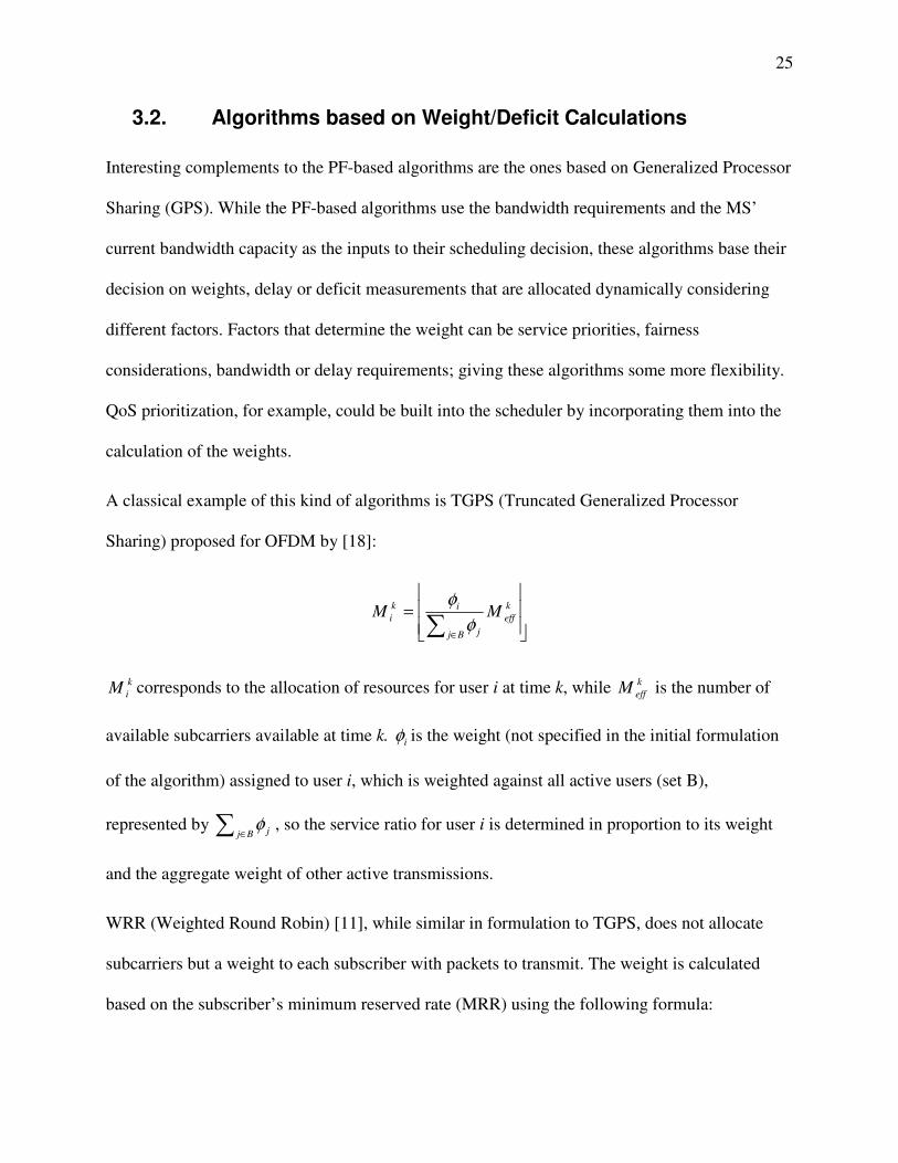
3.2. Algorithms based on Weight/Deficit Calculations
Interesting complements to the PF-based algorithms are the ones based on Generalized Processor
Sharing (GPS). While the PF-based algorithms use the bandwidth requirements and the MS’
current bandwidth capacity as the inputs to their scheduling decision, these algorithms base their
decision on weights, delay or deficit measurements that are allocated dynamically considering
different factors. Factors that determine the weight can be service priorities, fairness
considerations, bandwidth or delay requirements; giving these algorithms some more flexibility.
QoS prioritization, for example, could be built into the scheduler by incorporating them into the
calculation of the weights.
A classical example of this kind of algorithms is TGPS (Truncated Generalized Processor
Sharing) proposed for OFDM by [18]:
=∑ ∈
k
eff
Bj j
ik
i MMφ
φ
k
iM corresponds to the allocation of resources for user i at time k, while k
effM is the number of
available subcarriers available at time k. iφ is the weight (not specified in the initial formulation
of the algorithm) assigned to user i, which is weighted against all active users (set B),
represented by ∑ ∈Bj jφ , so the service ratio for user i is determined in proportion to its weight
and the aggregate weight of other active transmissions.
WRR (Weighted Round Robin) [11], while similar in formulation to TGPS, does not allocate
subcarriers but a weight to each subscriber with packets to transmit. The weight is calculated
based on the subscriber’s minimum reserved rate (MRR) using the following formula:

26
∑∈
=
nj
j
i
iMRR
MRRW , Wi is the weight assigned to user i, and n is the number of subscribers
The subscriber with the highest weight is then next in line to obtain bandwidth. While the
formulation is pretty simple, there are no considerations for a BE scheduling service, which does
not have specific MRR values.
Weighted Fair Queuing [19] (WFQ) assigns a weight to each subscriber the same way as WRR,
but the argument used to make a scheduling decision is the finish number, an estimation of the
time at which each individual packet will finish service. The packet with the lowest finish time
will be scheduled next. The finish number is calculated based on the subscriber’s weight, the
finish number of the previous packet scheduled on that connection and the length of the packet.
This algorithm was proposed for WiMAX OFDM in [11], at which point its complexity was
deemed high. In an OFDMA system, several connections can be served at once during a single
frame, which would require multiple rounds of the algorithm and hence higher complexity.
DRR (Deficit Round Robin) accounts for connections not scheduled, increasing a deficit counter
for each connection by a certain quantum unit. The deficit counter will be used in subsequent
scheduling rounds to compare to the size of the head-of-the-line (HOL) packet on each active
connection. If the connection’s deficit counter is larger than the HOL packet, it will be
scheduled, otherwise it will remain in the queue and the deficit counter will be increased by the
quantum while other connections are being served. DRR operates with packet sizes and relies on
knowledge of the head of line packet per connection, which is not known from the BS
perspective on the uplink. The algorithm in [20] presents a modified DRR algorithm for
WiMAX in which the quantum size is in units of slots, the queue sizes are converted from bytes
to slots based on the subscriber’s MCS and queue size is represented by virtual UL queues

27
created based on the UL bandwidth requests. The algorithm runs in several rounds until all
possible slots in the frame are allocated.
A variant of DRR is WDRR (Weighted DRR) also presented in [20], where preference is given
to connections with higher MCS by multiplying the quantum size (in slots) by bytes/slot
supported by the connection’s MCS and then dividing by six (which is the bytes per slot for the
most robust MSC: QPSK-1/2). This way connections with a higher MCS will have a bigger
quantum than connections with lower MCS and hence a higher probability of being scheduled
first.
A classical algorithm to deal with stringent delay requirements is Earliest Deadline First (EDF),
which assigns deadlines to packets on each connection and allocates bandwidth to the
subscribers based on such deadlines. It is then only applicable to UGS or rtPS scheduling
services that have specific delay requirements, but is a good candidate to be part of hybrid
algorithms that combine several scheduling solutions [21].
Highest Urgency First (HUF), presented in [22], is a modulation, latency and priority-aware
algorithm that builds on the fact that latency-dependent flows not necessarily have to be served
first as long as they are scheduled within their delay tolerance window. A deadline indicator,
calculated when packets arrive at physical queues on the downlink or virtual queues on the
uplink, is used for such purpose.
3.3. Opportunistic and Cross-Layer Algorithms
While the algorithms mentioned in the previous sections indirectly account for signal quality by
looking at the modulation supported by the subscriber (which at the end of the day is a function

28
of signal quality), the opportunistic algorithms in this section actually use the signal quality
reading (CNR, CINR, e-CINR, etc) as the argument used to make a scheduling decision.
Four well-known opportunistic algorithms that use signal quality as their basic input are
presented in [13]. They all are functions of signal quality, sharing the general form:
)(maxarg)(1
*
kiNi
k tXti≤≤
= ,
)( ki tX is the metric function, calculated at the beginning of time slot tk and )(*
kti corresponds to
the index of the user picked to be scheduled. Table 3.3-1 presents the 4 algorithms and the metric
used by each one.
In this category, cross-layer algorithms that incorporate both QoS-awareness and opportunistic
behavior are also considered. [13] further classifies these algorithms as non-queue aware, which
do not factor the influence of queue behavior on delay and hence on QoS, and queue aware,
which consider the effect of queue-related conditions in the behavior of the scheduler.
An algorithm that accounts for queuing delay, channel conditions and QoS prioritization (hence
making it a queue-aware cross-layer opportunistic algorithm) is Modified Largest Weighted
Delay First (MLWDF) [23], initially designed for CDMA systems, which has the following
formulation:
)()(maxarg)(1
*
kikiiNi
k trtWti γ≤≤
= ,
Where iγ corresponds to a priority factor, )( ki tW is the HOL packet delay (or queue length on
implementations that consider non-delay sensitive BE traffic [24] ) and )( ki tr is the channel
capacity with respect to flow i. By keeping an eye on queue states, as well as channel conditions,
the algorithm optimizes the throughput delivered to certain connections, while still keeping

29
queues from getting into a full congestion state. In fact, the authors claim that its behavior is
throughput optimal, maintaining all feasible traffic while still keeping all queues stable.
A WiMAX OFDMA version of MLWDF is presented in [24], extending the algorithm to relax
the priority constrains when delay sensitive traffic is far from approaching its deadline,
effectively giving some transmission opportunities to scheduling services that would usually
have to wait for the delay sensitive traffic to be scheduled first.
Table 3.3-1 Opportunistic Algorithms
Metric Algorithm
)( ki tγ CNS (Carrier to Noise Scheduling). Metric corresponds to CNR reading
for user i on time tk.
i
ki t
γ
γ )(
NCS (normalized CNR Scheduling). iγ corresponds to the average CNR
for user i. As CNS is too aggressive, scheduling always the highest
CNR reading, NCS introduces some fairness by scheduling the highest
normalized CNR on each time slot.
)(
)(
ki
ki
tT
tr
Proportional Fair Scheduling. This is the same algorithm described in
Section 3.1.
Max CNR in
each round
Opportunistic Round Robin (ORR). Users are scheduled in rounds of N
competitions. For the first time-slot in a round, the user with the highest
CNR is chosen. This user is then taken out of the remaining
competitions of the round, and for the next time-slot the user with the
highest CNR of the remaining users is scheduled. A normalized version
(N-ORR) that considers the normalized CNR as opposed to pure CNR
also exists.
3.4. Hierarchical / Hybrid Algorithms
Hierarchical/hybrid algorithms build on the fact that scheduling services have different and
sometimes conflicting requirements. UGS services must always have their delay and bandwidth

30
commitment met, so simply reserving enough bandwidth for those services and controlling for
oversubscription would be enough; rtPS or ertPS services have little tolerance for delay and
jitter, so an algorithm guaranteeing delay commitments would be more suitable; and finally, BE
and nrtPS will always be hungry for bandwidth with no considerations for delay, so a throughput
maximizing algorithm might be preferred.
While hierarchical refers to two or more levels of decisions to determine what packets to be
scheduled, hybrid refers to the combination of several scheduling techniques (EDF for delay
sensitive scheduling services such as rtPS, ertPS and UGS, and WRR for nrtPS and BE for
example). There could be hierarchical solutions that are not necessarily hybrid, but hybrid
algorithms usually distribute the resources among different service classes, and then different
scheduling techniques are used to schedule packets within each scheduling service, making them
hierarchical in nature. In [25], the authors use a first level of strict priority to allocate bandwidth
to UGS, ertPS, rtPS, nrtPS and BE services in that order; and then on a second level in the
hierarchy, different scheduling techniques are used depending on the scheduling service: UGS,
as the highest priority, has pre-allocated bandwidth, EDF is used for rtPS, WFQ for nrtPS, and
FIFO for BE. Similarly, [11] explains an algorithm that uses EDF for ertPS and rtPS classes, and
WFQ for nrtPS and BE classes.
In [26], the authors implement a two-level hierarchical scheme for the downlink in which an
ARA (aggregate resource allocation) component first estimates the amount of bandwidth
required per scheduler class (rtPS, nrtPS, BE and UGS) and distributes it accordingly. An
extended exponential rule algorithm is then proposed for rtPS and nrtPS, leaving scheduling of
BE and UGS as future research.
31
Even though admission control techniques are independent from the scheduling task, and could
be incorporated into any of the scheduling techniques presented so far, they are particularly
important for algorithms in this category. As certain scheduling services have higher priority
than others, starvation control has to be considered. Admission control, together with traffic
policing, is proposed in [25] and [26] implements an admission control module interacting with
the resource allocation module to dynamically decide if new connections are allowed.

32
4. Current Options for Mobile WiMAX Simulations
When one follows the evolution of scheduling solutions proposed, two parallel patterns starts to
emerge: One favoring simplicity and speed and the other one in favor of more elaborate
alternatives, with higher execution time and complexity. Simulations should help compare
schedulers that are simple in design and consider a few factors to more elaborate techniques that
consider a higher number of variables but have a higher complexity.
Several options to perform mobile WiMAX simulation are currently available. Initially, most
researchers used MATLAB to simulate portions of the WiMAX implementation, and later had to
write their own MAC/PHY implementation for end-to-end simulation tools like NS-2, Opnet and
Qualnet. Such implementations were not usually made publicly available, leaving no chance for
other researchers to replicate similar conditions for fair and unbiased comparisons of results.
Only until a couple of years ago commercial and open source solutions started to appear:
• Opnet released its WiMAX module in February 2006 and it has continuously improved it
since then. The latest release supports major features of the IEEE 802.16e PHY/MAC,
including all the scheduling services, radio link control, ARQ, MAC messaging, mobility
and OFDMA path loss model.
• Qualnet’s WiMAX module was introduced October 2006. Its latest release implements
all the WiMAX features mentioned for Opnet above, missing a security implementation
(PKM) and soft handoff.
• An ns-2 based WiMAX module is publicly available from the National Institute of
Standards and Technology (NIST) [27]. While the module is fairly well documented,
implements QoS, different scheduling services and mobility, it lacks OFDMA support,
making it usable for Fixed WiMAX simulation only.

33
• The Network and Distributed Systems Laboratory (NDSL) in Taiwan released an ns-2
based module in August 2006 [8]. The module had several releases adding QoS
parameters and OFDMA PHY scheduling services, but it does not implement mobility,
lacks documentation (as a matter of fact, their authors did not reply to any of the attempts
to contact them via e-mail) and a major issue has been identified by [28], causing the
scheduler not to account properly for the number of slots already allocated and hence
distribute an unlimited amount of resources.
• An ns-2 based WiMAX module is being developed for the WiMAX forum by several
universities including the Network and Distributed Systems Laboratory (NDSL),
Washington University in St. Louis (WUSTL), Rensselaer Polytechnic Institute (RPI)
and the Wireless Internet and Networks Laboratory (WiNE). This module would have
been ideal for the current research, but unfortunately it is not yet completed and the
forum will initially make it available to WiMAX forum members only.
4.1. Mobile WiMAX Simulation in Qualnet
Given the lack of availability of a reliable open source tool for mobile WiMAX scheduling
simulations, only commercial alternatives can be considered at this time. Qualnet’s Advanced
Wireless Model [29] was chosen for this research due to the flexibility of their research license
(Opnet only allowed their software to be installed on-campus while Qualnet offered an option to
run a license server on-campus and a Qualnet client off-campus) and the features currently
implemented:
• OFDMA PHY. Very important for realistic simulation of mobile WiMAX, which
requires multiple access both on downlink and uplink.

34
• MAC messaging: ranging, bandwidth request/allocation, handover, sleep mode, paging,
power control.
• Adaptive modulation and coding (AMC) to allow BS and subscribers to change their
modulation according to radio link conditions.
• Mobility support. Will allow scenarios under mobility conditions. A great advantage over
the ns-2 based module available from NDSL which allowed testing under stationary
conditions only.
• Support for all five service classes (UGS, ertPS, rtPS, nrtPS, BE) specified in the
standard.
• Basic admission control via a token bucket mechanism. Important as some of the
proposed algorithms operate in conjunction with admission control.
The current scheduling algorithm implemented in Qualnet’s simulation software is a hierarchical
algorithm (hierarchical, but yet not hybrid and a single algorithm is used) using strict priority
combined with a basic WFQ scheme.
Strict priority initially classifies the connections according to their scheduling service and serves
them in order: UGS, ertPS, rtPS, nrtPS and BE. There is then no consideration for delay
requirements as even connections that have packets reaching their delay deadline in ertPS or rtPS
queues will not be served until the UGS queue is empty. Moreover, packets in nrtPS or BE
queues could potentially starve if admission control were not implemented.
Within each scheduling service, WFQ chooses the next packet to be scheduled using a basic
formulation:
=∑∈Nj
j
i
w
wSSi
*,

35
Here wi is the weight of each connection, calculated based on its bandwidth requirements. S and
Si are the total number of slots to be distributed and the number of slots assigned to connection i
respectively. N is the set of all connections with packets waiting to be scheduled.
4.2. Limitations of Qualnet Simulator
There are still some limitations to Qualnet’s simulation software in regards to certain WiMAX
features not yet implemented, or partially implemented, which should be considered in the
context of this research:
1. There is no authentication or traffic encryption. While not having authentication will only
imply not having MAC authentication messages during network entry or handoff, there is a
direct impact on the throughput obtained as additional overhead is introduced when
encryption over the air is enabled. All throughput numbers produced in this research will not
consider encryption a part of the equation.
2. Packet header compression is not implemented. Although it should not directly impact the
behavior of a certain scheduler vs. another one, it is a consideration when reading throughput
numbers.
3. The currently implemented WFQ scheduler does not consider priorities among connections
within the same scheduling service.
4. Uplink bandwidth scheduler is not implemented as an API. While the downlink scheduler
uses a well-defined API to perform scheduling tasks such as adding packets to queues,
setting and retrieving current priorities of the queues and adding changes to modify the
behavior of the scheduler, the uplink direction is implemented over several files and
hundreds of lines of code with no documentation. Writing schedulers for both uplink and

36
downlink direction would then imply working on not three but six schedulers, which is not
achievable within the time planned for this research.
5. Applications’ QoS parameters are not configurable. QoS parameters are actually determined
based on the configured application. In the current release, only CBR and VBR applications
map properly to their corresponding QoS parameters. As an example, a CBR application
configured to send 128 bytes packets every second would map to the following QoS
parameters:
maxSustainedRate = 1024 bps (128 bytes/second * 8 bits/byte)
minReservedRate = 1024 bps
maxLatency = 1000000000 (1000 ms)
toleratedJitter = 0 (0 ms)
This seems pretty convenient as service flow parameters are automatically configured, but
limits the number of applications that can be properly simulated. Voice over IP for example,
is mapped only partially. A voice over IP application, using a G.711 codec which requires at
least 64 kbps before overhead is mapped to the following QoS parameters:
maxSustainedRate = 800 bps
minReservedRate = 800 bps
maxLatency = 100000000 (100 ms)
toleratedJitter = 100000 (0.1 ms)
Such a flow is not enough to carry the voice over IP traffic, as it results in a considerable
uplink delay and packet drops when ertPS or UGS service flows that rely on pre-allocated
bandwidth to deliver their data are used. Not using UGS or ertPS for voice traffic, however,
would eventually have a negative impact as latency could not be guaranteed and the traffic
would be competing with throughput-intensive applications. This is another reason for
limiting the scope of the simulations to downlink only as the configured QoS parameters
could not be used for uplink VoIP traffic without some rework to either map the service flow

37
properly or implement a way to configure the QoS parameter independently from the
application.
Other important applications such as FTP and HTTP suffer the same limitation. FTP and
HTTP applications for example do not map to any QoS parameters and there is no way to
manually configure them, so it is not possible in the current implementation to configure
HTTP in a service class different from BE.
4.3. Qualnet's WiMAX Scheduler
A UML diagram of the current WiMAX Scheduler implementation for WFQ can be seen in
Appendix A. All schedulers, including the ones that will be implemented as part of this research,
derive from the root Scheduler class, which defines the basic member functions that all scheduler
must implement: scheduler initialization, add and remove queues, and insert/dequeue packets
from to/from a specific queue. Depending on the implementation, additional data structures and
variables to keep track of counters, weights, ratios and flags will be required.
For a WiMAX downlink scheduler, the MacDot16Bs structure contains a pointer to a structure of
Scheduler type which is initialized as part of the instantiation of the WiMAX MAC, and all the
required member functions to create/delete queues and insert/retrieve packets to/from the queues
are accessed from there. A scheduler has a number of queues, each one corresponding to a
WiMAX CID. Each queue then has a dynamic array which stores the packets that need to be
scheduled.
Every time a new downlink WiMAX connection is established, a temporary queue is created to
store packets sent to that connection while a new queue is added to the scheduler. Once the
queue has been setup, packets from the temporary queue are then moved over and any
subsequent packets arriving for that connection will be enqueued using the insert member

38
function. It is then up to the scheduler to decide what queues to serve on each scheduling cycle
and call the retrieve function to do so.
Qualnet implements the WFQ algorithm in the WfqScheduler class, derived from the
FQScheduler class. The FQScheduler class exists to provide some common functionalities to
other weight-based schedulers, so only the specifics of the insert and retrieve member functions
(which are particular to WFQ) need to be implemented.
The process of scheduling a downlink subframe is shown in Figure 4.3-1. Every 5ms (the
configured frame duration) a new MAC frame has to be built, so a function is called to reset all
the previous downlink and uplink allocations. Uplink allocation happens first, in order to
determine the size of the uplink map, and the number of slots that will be left to build the
downlink map and for data allocations. When the ScheduleDlSubframe function is called, the
data schedulers (one for each scheduling service) will be checked in order to determine if there
are any queues requiring service. Only when all the queues in a higher priority scheduling
service are empty, the next priority scheduler will be served. The process will continue until no
more slots are available or until all queues have been served.
Figure 4.3-1 Scheduling a Downlink Subframe

39
The process of building the DL subframe is not linear, every time slots are allocated a check has
to be made to ensure that the capacity of the sub frame will not be exceeded when mapping
overhead is added. If that check fails, the frame is considered full and the last packet that was
supposed to be added to the subframe is left on the scheduler. Once the contents of the DL
subframe have been defined, the MAC frame including UL and DL maps as well as downlink
data is built and passed to the PHY layer for transmission. The process will start over in the
subsequent scheduling cycle.
40
5. Scheduling Design Dimensions
We have summarized scheduling solutions for mobile WiMAX and have produced a taxonomy
that classifies the protocols in four categories, according to their underlying formulation: Balance
fairness and throughput, weight/deficit based, opportunistic/cross-layer, and hybrid/hierarchical.
While such a classification is not perfect, it contrasts with [11], which categorizes solutions into
homogenous (protocols based on legacy techniques adapted to WiMAX), hybrid (a combination
of homogenous protocols) and opportunistic (algorithms exploiting channel conditions although
some homogenous techniques already do that), and with [12], which follows the evolution of
different scheduling protocols over time.
Several interesting conclusions can be drawn from reviewing the literature:
1. The scheduler problem can be seen as the combination of three interdependent problems:
choosing which connection to serve next, choosing the right modulation for the data and
fitting corresponding bursts on the frame. The current research will focus mostly on the
first issue, comparing four promising scheduling techniques found in the literature: WFQ,
PF, MLWDF and HUF.
2. A complete end-to-end scheduling solution should account for admission control and
traffic shaping.
3. Scheduling in WiMAX OFDMA can be summarized as meeting QoS commitments while
trying to maximize sector throughput. The scheduling algorithms chosen for
implementation do precisely that one way or the other.
4. Scrutinizing current scheduling alternatives under the same conditions is ideal to have a
more realistic comparison of the performance of each algorithm.

41
5.1. Scheduling Subproblems
Figure 5.1-1 presents a high level view of the scheduling process in WiMAX, depicting the three
decisions that need to take place. Physical queues are maintained for the downlink direction for
each scheduling service, while virtual queues are maintained in the uplink direction based on
bandwidth requests coming from the mobiles or the configured sustained traffic rate for UGS and
ertPS. It is up to the scheduler in each direction to sort through those queues and pick a subset of
PDUs to be scheduled. Uplink packets update the virtual queues and uplink modulation and a
feedback loop exists between the subscriber and the BS in order to identify the modulation to be
used in the DL direction.
In addition to having to take care of building the DL/UL maps, the 2D mapper entity has to
accommodate the PDUs within bursts per subscriber that will later constitute the downlink
subframe. During the 2D mapping process, some portions of a PDU might not fit entirely so they
will have to be sent back to the scheduler to be processed during the next round.

42
Figure 5.1-1 High Level View of Scheduler
According to [6] and [30], there is a circular dependency between those processes that should be
broken somewhere. While [30] proposes to first choose the next connection to be scheduled, then
the modulation, and finally the frame fitting process, [6] prefers the approach of treating the
modulation as an exogenous process and then breaking down the scheduling problem into two
sub-problems:
a. Macro scheduling. Assume that a certain profit for transmitting a frame as well as the
modulation to be used has been previously assigned to each connection. The authors
formulate this problem as a multiple choice knapsack [31] with s1 …sm PDUs, a
capacity C (number of slots on a frame) and each PDU having a well-known

43
modulation and coding rate (the weight w(si)) and a profit (p(si)) and propose an
approximation algorithm that runs in polynomial time.
b. Micro scheduling. A decision as to how to build the frame is made based on a greedy
algorithm that locally minimizes the wasted space.
For the simulations in this research, the approach proposed by [6] of assuming the modulation as
an attribute of the connection checked at scheduling time will be adopted. It is also important to
highlight that while the process of 2D mapping is required for any implementation of an
OFDMA scheduler, most papers do not elaborate on how their algorithm is to build the DL/UL
subframes and how to deal with unused slots and bumped PDUs due to frame fitting. Given such
limitations, the current research will focus on the problem of choosing the PDUs to be scheduled
over the air, conserving the frame fitting technique already implemented in the Qualnet
simulation software.
5.2. Admission Control and Traffic Shaping
Admission control and traffic shaping should also be contemplated as part of the end-to-end
scheduling solution that requires enforcement of a maximum sustained traffic rate. Even a well-
engineered network can suddenly start running out of sector capacity if RF conditions change. In
such situations, a well-defined algorithm that decides which connections should stay up and
which ones to drop or lower their bandwidth is important.
In [32], the authors propose a hierarchical algorithm for admission control that first assigns
thresholds to each scheduling service and then decreases a capacity counter per scheduling
service every time a new connection is accepted. Even though a scheduling service can exceed
its threshold, its priority to access the capacity will decrease and eventually could get some of its
44
connections dumped if a need arises. There is also a provision for traffic policing using a token
bucket mechanism. There is no reason why such an approach could not be combined with any of
the scheduling algorithms to provide a complete solution to the scheduling problem.
5.3. Meeting QoS while Maximizing Throughput
Scheduling in WiMAX OFDMA can be summarized as meeting QoS commitments while still
maximize sector throughput. Chosen alternatives use different approaches to achieve that double
goal.
Fairness is an important factor as sector capacity cannot be maximized to a point where
connections that have poor conditions starve and do not have any service, but at the same time
subscribers with poor conditions should not be allowed to dramatically decrease the sector
capacity. Figure 5.3-1, inspired by [17], illustrates the issue of poor vs. good conditions. It can be
seen, for example, that in order to reach a sector throughput around 4,9Mbps using QPSK ½
modulation would require over 500 slots, while when using an average modulation like 16QAM
½ about 250 slots are required. This would then increase the sector capacity as the remaining
slots can be used for other subscribers, or to supplement the current transmission with additional
bandwidth. A more efficient modulation like 64QAM ½ would use only a little over 100 slots,
versus more than 500 slots using QPSK ½.
On the other hand, some of the algorithms found in the literature, while interesting, do not have
any consideration for meeting QoS requirements, which make them impractical for a real
WiMAX implementation and are considered incomplete for the purpose of this research.

45
Figure 5.3-1 Spectral Efficiency of Different Modulations
5.4. The Need for Realistic Scenarios
Most papers that proposed new algorithms only compare themselves to the two extremes of the
spectrum: max Carrier to Interference (C/I) ratio (allocating resources to the subscriber with the
best RF conditions at a given time) and FQ (allocating resources equally no matter the
modulation being used). While this is important from a baseline perspective, those algorithms do
not satisfy QoS requirements, so they could not be possibly implemented in real life.
Furthermore, they represent the maximum and minimum bound of performance and one would
expect that any new scheduling solution would be somewhere in between these two extremes.
The value of this research is in (1) testing several recent OFDMA WiMAX scheduling proposals
under the same conditions, so more realistic conclusions can be drawn and (2) going through the
implementation of the actual pseudo-code proposed, highlighting assumptions that would not
hold ground in an actual implementation. A similar objective is pursued in [33], where a
Number of slots per modulation scheme
0
100
200
300
400
500
600
1,536,000 1,843,200 2,457,600 4,915,200 sector throughput (bps)
Based on DL PUSC with 5 ms frame duration
Number of Slots
QPSK 1/2
QPSK 3/4
16QAM 1/2
16QAM 3/4
64QAM 1/2
64QAM 3/4
64QAM 5/6

46
comparison of three allocation schemes was performed using the same simulation tool but once
again several reasons make the algorithms in that paper not feasible for real deployment :
– Max Waiting Time: The connection with the largest waiting time for the HOL packet is
selected. It is basically an EDF implementation, but all connections are treated the same as
there are no considerations for different QoS parameters.
– Round Robin: A connection is selected in classical Round Robin manner. Once again QoS
parameters are not considered and there is no balance between fairness and throughput.
– Max SINR Gain: Unlike the other two schemes, this strategy finds the optimum resource-
connection pair. Each resource is assigned to the connection with the highest SINR gain
compared to the mean SINR. Such an algorithm, if implemented as-is, would simply starve
connections with poor RF conditions.

47
6. Detailed Description of Selected Scheduling Algorithms
In addition to WFQ, the scheduling algorithm already implemented in Qualnet which will be
used for initial simulations, three algorithms have been chosen for implementation in the Qualnet
simulation software: Proportional Fairness (PF), a well-known algorithm that balances fairness
and throughput adapted to Mobile WiMAX by [17] ; multiclass MLWDF [24], a hierarchical,
cross-layer, queue-aware opportunistic algorithm with two implementations: one using strict
priority among the scheduling services, and another one relaxing the priority leaving some BE
and nrtPS traffic to go through first when UGS and rtPS traffic is far from reaching its delay
expiration; and Highest Urgency First (HUF) a weight-based, hierarchical, modulation, latency
and priority-aware algorithm that reserves bandwidth for the more urgent requests and allocates
the rest according to additional criteria.
The algorithms were chosen for multiple reasons. For starters, only a few of the algorithms
surveyed are suitable for implementation as most do not meet the requirements of Mobile
WiMAX. Second, several basic algorithms like WRR, RR and FQ [11][12][13] and some legacy
algorithms like DRR, WDRR [20] and MLWDF [24] have already been tested in the context of
Mobile WiMAX in previous research, so not many additional insights are expected from
implementing them. Third, two of the chosen algorithms, namely Multiclass MLWDF and HUF,
incorporate a novel concept not seen in other papers: they contemplate deferring the transmission
of delay sensitive traffic until their delay commitment is close to expiration, hence favoring
throughput-optimizing scheduling services. Analyzing the throughput improvement of such an
approach while comparing its accuracy in meeting delay commitments is an interesting
deliverable of the current research.

48
For a full scheduling implementation, a hybrid approach could be more convenient given the
different requirement of each WiMAX scheduling class. We however decided in favor of testing
each scheduler performance individually, in order to identify the strengths and weaknesses of
each implementation.
6.1. Weighted Fair Queuing
Qualnet's scheduler implementation for WiMAX is based on the Weighted Fair Queueing
(WFQ) algorithm, widely implemented over WAN links thanks to Cisco, which uses it as the
default queuing mode on most T1/E1 serial interfaces [34].
WFQ is an algorithm based on weight calculations, derived from the General Processor Sharing
(GPS) algorithm. As mentioned in Chapter 3.2, WFQ uses a metric called finish number, which
is an estimation of when the HOL packet for a certain queue will finish its transmission and is
defined for the kth packet in the ith queue as :
F(k,i) = S(k,i) + L(k,i)/W(i),
Being F(0,i)=0;
S(k,i) = max [F(k-1,i) , RoundNumber], called the start number ;
L(k,i) the length of packet k in queue i;
and W(i) the weight of queue i.
RoundNumber represents the progression of virtual time, increased in each scheduling cycle, and
is defined as:
RoundNumber(t)=RoundNumber(t-1)+RoundRate(t);
RoundRate(t)=1 / (Sum of active queues' weights at time t)
A queue is defined as active if it is not empty and its weight for the WiMAX implementation is
the normalized minimum reserved traffic rate (MRTR) expressed as:
W(i)=MRTR(i)/(Sum of MRTR for all queues)
49
Finally, the WFQ scheduler will serve the queue whose HOL packet has the smallest finish
number.
Assuming a fixed packet size for all connections, queues will be served at about a rate equal to
W(i), their normalized MRTR. This behavior can be observed with a synthetic example,
presented in Table 6.1-1, where queue 1 has a weight that is half the weight of queue 2, and in
each cycle there is a new packet of size 1 in each queue .
Table 6.1-1 WFQ Behavior
RoundRate-> 1 2 3 4
Queue 1
L(k,1)=1,
W(1)=1/3,
L(k,1)/W(1)=3
Pkt# 1 2 3
S(k,1) 1
F(k,1) 4
Pkt# 1 2 3
S(k,1) 1 4
F(k,1) 4 7
Pkt# 2 3
S(k,1) 4 7
F(k,1) 7 10
Pkt# 2 3 4
S(k,1) 4 7 10
F(k,1) 7 10 13
Queue 2
L(k,2)=1,
W(2)=2/3,
L(k,2)/W(2)=1.5
Pkt# 1 2 3
S(k,1) 1
F(k,1) 2.5
Pkt# 2 3
S(k,1) 2.5
F(k,1) 4
Pkt# 2 3
S(k,1) 2.5 4
F(k,1) 4 5.5
Pkt# 3 4 5
S(k,1) 4 5.5
F(k,1) 5.5 7
Served queue Queue 2 Queue 1 Queue 2 Queue 2
WFQ's behavior is ideal in a wired scenario: It will fairly distribute the available bandwidth to all
the active flows, by giving each flow the proper priority as indicated by its weight. On the other
hand, flows that try to exceed their traffic rate will suffer the consequences as they will be
limited by their defined weight. Finally, low volume traffic streams will benefit as they will be
able to quickly complete their transaction without much impact on high volume applications. It
will be demonstrated later that these benefits come at a disadvantage in the wireless
environment, as connections that exhibit poor RF conditions will be treated the same as
connections that do not, effectively lowering their efficiency.

50
6.2. Proportional Fairness
Proportional Fairness (PF) [20] is the most representative example of algorithms that balance
throughput and fairness. PF is used in CDMA networks and several current implementations of
Fixed and Mobile WiMAX, so it serves as a good, realistic baseline to compare other algorithms.
PF assigns slots to connections with the best ratio of achievable rate per slot, Di(t), over the
previously achieved rate, Ri(t), according to the following formulation:
)(
)(maxarg
1 tR
tDj
i
i
Ni≤≤
= ,
Di(t) is the number of bytes supported by the current modulation of connection i and Ri(t) is the
averaged rate, in bytes per slot, given to connection i using the following formulation:
)(*1
)1(*)1
1()( tDt
tRt
tR i
c
i
c
i +−−= , if the connection was just served,
)1(*)1
1()( −−= tRt
tR i
c
i , Otherwise.
Connections with good Di(t) will get preference, but as connections with a bad Di(t) start to be
underserved, the Ri(t) factor will start to gain weight and influence the value of the ratio. Ri(t) is
an exponential moving average [35], with a smoothing factor α=1/ tc. Parameter tc, called the
observation window, is a unit-less time constant that helps tune the tradeoff between throughput
and fairness. The effect of tc on the PF ratio can be seen using a synthetic example assigning
only one slot to either a 64QAM or a QPSK connection during each scheduling cycle as shown
in Figure 6.2-1 to Figure 6.2-4. Assuming RF conditions remain the same, leaving Di(t)
unchanged, a smaller tc value will make the Ri(t) factor decrease faster (Figure 6.2-1) and the PF
ratio will increase (Figure 6.2-2), making connections with bad RF conditions more likely to be

51
served. Bigger tc values will do the opposite: Ri(t) (Figure 6.2-3) will decrease and the PF factor
(Figure 6.2-4) will increase slower, delaying the scheduling cycle at which the connection with
worse RF conditions is served.
Figure 6.2-1. Behavior of Ri(t) with tc=80

52
Figure 6.2-2 Behavior of PF Ratio for tc=80
Figure 6.2-3 Behavior of Ri(t) for tc=140

53
Figure 6.2-4 Behavior of PF Ratio for tc=140
The authors in [20] make several assumptions to accommodate the protocol to the particulars of
WiMAX:
• The initial averaged rate Ri(0) is obtained based on the sector average rate divided by the
expected number of connections.
• Consider tc values between 100 and 100000 slots, which for an average number of slots of
500 per DL or UL subframe and a 5ms subframe would correspond to values between
100*(5ms/500 slots)=1 ms and 100000*(5ms/500 slots)=1 second.
• As prioritization is not contemplated in this algorithm, a hierarchical approach is used:
management data and UGS are always served first, and then on strict priority ertPS, rtPS,
nrtPS and BE respectively. The PF scheduler is applied to the four later scheduling
services.

54
The premise of PF is simple, yet elegant: Give preference to the flow with best channel
conditions in order to maximize the use of the spectrum and have that flow finish first, but at the
same time conserve fairness by keeping track of how long flows with poor channel conditions
have been without service and allowing to fine-tune the behavior by modifying the value of the
unit-less parameter tc. This can be seen in operation in Figure 6.2-5 with an extreme example
using the PF scheduler implemented as part of this thesis: Two subscribers (SSs) running each an
FTP transfer start at the same time, one of the subscribers has perfect channel conditions and a
modulation of 64QAM 3/4, while the other is in conditions that yield QPSK 1/2 modulation
only. It can be observed how the scheduler gives preference to the flow with higher slot
efficiency, allowing it to complete its data transfer quite rapidly, while the flow with lower slot
efficiency goes without service.

55
Figure 6.2-5 Goodput for Subscribers Under Different Channel Conditions PF tc=100K
The amount of time a service will go without service can be tuned by setting tc, the observation
window parameter. Figure 6.2-6 shows the same run, this time with a tc value that is half of the
value configured for the previous figure. It can be seen how at about half of the transmission
time of the flow with better modulation, slots start to be assigned to the subscriber with worse
modulation, and the available resources start to be shared among the two flows.
Goodput over time PF Scheduler (Tc=100K) Controlled environment
0
2,000,000
4,000,000
6,000,000
8,000,000
10,000,000
12,000,000
14,000,000
16,000,000
18,000,000
20,000,000
15.5 16 16.5 17 17.5 18 18.5 19 19.5 20 20.5 21 21.5 22 22.5 23 23.5 24 24.5 25 25.5 26 26.5 27 27.5 28 28.5 29 29.5 30
Simultaneous FTPs among 2 SSs with different channel conditions
Mbps
SS1_QPSK1/2 SS2_64QAM3/4

56
Figure 6.2-6 Goodput for Subscribers Under Different Channel Conditions PF tc=50K
One can see the dramatic contrast of the scheduling decision when running the same FTP test
using the Weighted Fair Queue (WFQ) implemented in Qualnet (Figure 6.2-7). It can be seen
how the flow for SS number 2 gets constrained by the slots being assigned to SS number 1,
effectively lowering its achievable throughput and causing TCP to slow down and having both
flows terminate at about the same time. While the improvement in sector throughput using the
PF scheduler is considerable, in real life flows are usually limited in how much throughput they
can achieve by their Maximum Sustained Traffic Rate (MSTR) parameter. The impact of this
constrain will be explored further in the simulation results section.
Goodput over time PF Scheduler (Tc=50K) Controlled environment
0
2,000,000
4,000,000
6,000,000
8,000,000
10,000,000
12,000,000
14,000,000
16,000,000
18,000,000
20,000,000
15.5 16 16.5 17 17.5 18 18.5 19 19.5 20 20.5 21 21.5 22 22.5 23 23.5 24 24.5 25 25.5 26 26.5 27 27.5 28 28.5 29 29.5 30 30.5
Simultaneous FTPs among 2 SSs with different channel conditions
SS1_QPSK1/2 SS2_64QAM3/4

57
Figure 6.2-7 Goodput for Subscribers WFQ Scheduler
6.3. Multiclass MLWDF
Multiclass MLWDF [24] is a cross-layer, queue aware opportunistic algorithm with several
improvements over the original MLWDF algorithm proposed in [23]: Multiple traffic classes as
well as multi-channel connections are considered. The main improvement, which makes it an
interesting candidate for implementation, is relaxing the strict priority constrain imposed by
having packets with QoS requirements always scheduled over packets without any QoS
requirements. That is, if QoS packets still have a long time-to-live, such packets can be delayed a
little and in the meantime BE packets are scheduled instead of having to wait in favor of the
delay-sensitive traffic.
Goodput over time WFQ Scheduler Controlled environment
0
2,000,000
4,000,000
6,000,000
8,000,000
10,000,000
12,000,000
14,000,000
16,000,000
18,000,000
20,000,000
15.5 16 16.5 17 17.5 18 18.5 19 19.5 20 20.5 21 21.5 22 22.5 23 23.5 24 24.5 25 25.5 26 26.5 27 27.5 28 28.5 29 29.5 30
Simultaneous FTPs among 2 SSs with different channel conditions
Mbps
SS1_QPSK1/2 SS2_64QAM3/4

58
The authors propose a scheduler based on the HOL delay for QoS based scheduling services and
queue length for BE and nrtPS traffic. The QoS scheduler has priority over BE, an enhanced
implementation called Joint Scheduler (JS) is proposed to relax this rule and schedule BE traffic
together with QoS traffic when the QoS packets are far from their delay expiration. They use a
50% heuristic (if delay is less than 50% of the deadline, BE packets will be scheduled over QoS
packets) to perform such decision. The pseudo code of the proposed implementation is shown
below.
At each scheduling instance {
for j=1 to N { update CR(j), QLB(j), QLQ(j) and WT(j)
AR(j) = w*AR(j) + (1-w)*CR(j) }
QoS_schedule = 0
for j=1 to N {
if (WT(j) > x*MD(j)) { QoS_schedule = 1 }
}
if (QoS_schedule > 0){SM= arg max j ( CR(j)/AR(j)*WT(j)/MD(j) )
else { SM = arg max j ( CR(j)/AAR(j)*(QLQ(j) + QLB(j))) }
for j=1 to N {
if (SM== j) { AAR(j) = w*AAR(j) + (1-w)*CR(j) }
else {AAR(j) = w*AAR (j) } }
}
< Variables>
AAR(j) : Moving average of MS j's allocated channel rate (bits)
AR(j) : Moving average of MS j's CR(j) (bits)
CR(j) : MS j's current channel rate (bits)
MD(j) : Maximum allowed delay of MS j's QoS class connection (ms)
N : Number of active queues
QLB(j) : MS j's BE class queue length (bits)
SM : Index of the selected MS
w : Weighting factor, used value is 0.99
WT(j) : Waiting time of Head-of-line packet in the MS j's QoS class queue
QLQ(j) : MS j's QoS class queue length (bits)
x : threshold parameter, used value is 0.5

59
A couple of parallels can be drawn between MLWDF and PF. For starters, they both consider the
connection's modulation efficiency as part of their scheduling decision; secondly, they both use
an exponential moving average to keep track of the progression of achieved rate. However,
MLWDF's ratio is different for QoS-aware connections (UGS, ertPS, rtPS), and it also uses
additional metrics for its calculation. A closer look at the algorithm above reveals that there are
actually two ratios, one to be used for QoS-aware connection:
)(
)(*
)(
)(maxarg
1 jMD
jWT
jAR
jCRSM
Nj≤≤
= ,
where the HOL Packet's Waiting Time to maximum delay ration is considered; and another one
for non-QoS connections:
)()(*)(
)(maxarg
1
jQLBjQLQjAAR
tCRSM
Nj
+=≤≤
,
where the number of enqueued bytes both for QoS-aware and non-QoS-aware connections for
that subscriber are considered.
In summary, Multiclass MLWDF behaves similarly to PF, giving preference to connections with
good RF conditions first. In addition, QoS-aware connections are delayed in favor of non-QoS-
aware ones when they are far from violating their delay commitments. It will be seen in the
results section that this actually improves throughput performance, with the effect of adding
extra delay on QoS-aware connections.
In the real world, major adjustments would be required to come up with a full implementation of
this scheduler: The scheduler only contemplates the downlink direction, for which HOL delay
and queue length can be easily calculated. In the uplink direction, virtual queues represent the
load of a specific connection and the HOL delay is calculated from the moment a bandwidth
request is observed for that connection, so maintaining the accuracy of the information is not

60
trivial and would represent a considerable challenge for connections with stringent delay
requirements.
6.4. Highest Urgency First
HUF [22] is a hierarchical algorithm in the sense that there is a first level that schedules all
connections according to their deadline (in order to guarantee QoS commitments) and allocates
the remaining bandwidth to the HOL packet on the queue with the highest AverageUFactor.
The algorithm is also weight-based in the sense that it relies on an urgency indicator to make
scheduling decisions. The urgency indicator (called UFactor) considers latency requirements,
priority and modulation of packets in a connection and is formulated as follows:
i
ji
jiD
PN )1(*Ufactor ,
+= , where
==
ratecodingperbytes
etSizeofPackrequiredslotsofN i
i___
__# , and
−
=
otherwise
ionFrameDurat
MaxLatency
Di
,1
, for real time applications
Parameter i corresponds to the packet index, j is the queue or connection, and Pj is the priority of
each connection, a configurable parameter from 1 to 7. HUF was the only algorithm found in the
literature that explicitly contemplates the connection's priority as part of its scheduling decision.
Having the UFactor for each packet, the AverageUFactor is calculated for each queue, and the
queue with the highest AverageUFactor will be served.
The AverageUFactor for queue j is calculated as follows:

61
n
factorUn
i
ji∑=
−
= 1
,
jfactor-AverageU ,
Where n is the number of requests (i.e. active packets on the queue ready to be served) on the
queue and UFactori,j corresponds to the ith request on queue j. Head-of-the-line requests for
each queue are then dispatched in decreasing order of AverageUFactor. Only the HOL request
of each connection is served each time, so if there are any slots left after all the queues have been
dispatched, the AverageUFactor will be recalculated for all queues and the remaining bandwidth
will be allocated accordingly. The algorithm can be summarized as follows:
At each scheduling cycle {
for j=1 to N {
for each packet i on queue j {
deadline(i,j)=deadline(i,j)-1
if (deadline(i,j)==1 and slots_available>=slots_required(i,j)) {
dispatchPacket(i,j)
slots_available=slots_available - served_slots(j)
}
}
}
while (slots_available>0)
{
for j=1 to N {
AverageUFactor(j)=0
for each packet i on queue j {
update_U_factor(i,j);
AverageUFactor(j)= AverageUFactor(j)+UFactor(i,j)
}
AverageUFactor(j)= AverageUFactor(j) /NumPackets(j)
}
SM=argmax j (AverageUFactor(j))
Serve_slots(SM)
slots_available= slots_available-served- served_slots(SM)
}
<Variables>
deadline(i,j) : Deadline of packet i on queue j
slots_available : Number of slots left on current scheduling cycle
slots_required(i,j) : Slots required to transmit packet i on queue j

62
served_slots(j) : Number of slots served to queue j
AverageUFactor(j) : Average U Factor of queue j
NumPackets(j) : Number of packet on queue j
UFactor(i,j) : U Factor of packet i on queue j
N : Number of active queues
SM : Index of the selected MS

63
7. Simulation Parameters
Several efforts have been made to follow standard guidelines to make results as comparable as
possible: First, system parameters in Section 7.1 reflect the default values specified by the
WiMAX Forum; second, based on the defined system parameters, theoretical maximum
throughput numbers have been calculated in Section 7.2 in order to have a proper baseline for
further evaluations; third, in Section 7.3 two scenarios are proposed: one simulating a closed-
loop environment under which signal levels and modulation schemes are kept constant, and
another scenario in which a Rayleigh fading model is introduced to simulate an urban pedestrian
environment, creating variability on reception levels and modulation schemes used by the
subscribers.
7.1. WiMAX-specific System Parameters
In order to have a scenario as realistic as possible to what initial WiMAX deployments will be
using, the WiMAX system parameters were chosen according to the recommended default
values from the WiMAX Forum Mobile System Profile [5] which lists all the WiMAX system
parameters, their status (mandatory, potential mandatory or optional), and their supported value
and valid combinations with other parameters. Table 7.1-1 lists relevant parameters as well as the
chosen value for the Qualnet simulation.
While most of the parameters align with what is specified in the Mobile System Profile, H-ARQ,
authentication and encryption, are not supported by the Qualnet simulation software.
Fragmentation was initially enabled, but had to be disabled as a bug was found causing queue
leaks when fragmentation was taking place. Also, in order to be able to properly characterize the

64
behavior of the different schedulers, ARQ was disabled so retransmissions do not occur when
packets are discarded.
Table 7.1-1 WiMAX Simulation Parameters
System Parameter Value
PHY Mode OFDMA
Band Class frequency range 2.3 – 2.5 GHz
Channel Bandwidth 10 Mhz
FFT size 1024
Duplexing mode TDD
Sampling Factor 28/25
Cyclic Prefix 1/8
Frame length 5 ms
TTG 10 µs
RTG 10 µs
SSTG 4 µs
Number of symbols per frame 47
DL / UL symbol ratio 32/15
Number of subchannels on downlink direction 30
Number of subchannels on uplink direction 35
DL subcarrier allocation scheme PUSC
UL subcarrier allocation scheme PUSC
Initial ranging in PUSC zone with 2 symbols YES
Periodic ranging in PUSC zone with 1 symbol YES
BW request in PUSC zone with 1 symbol YES
ARQ and H-ARQ Disabled
Authentication Disabled
Encryption Disabled
Fragmentation Disabled
7.2. Maximum Throughput Calculations
As mentioned in Section 2.1, a slot is constituted of a number of subcarriers over several
symbols. In the case of DL PUSC, a slot is composed of 24 data subcarriers over two symbols,
so a total of 48 data subcarriers per slot can be modulated in order to transmit a stream of bits. As
shown in Table 7.2-1, knowing how many bits can be transmitted for each modulation, one can

65
obtain the number of bits that can be carried in a slot depending on the modulation and coding
scheme.
Table 7.2-1 Bits per Slot for each Modulation and Coding Scheme
Modulation Bits/symbol Coding Bits/slot
1/2 2x1/2x48=48 QPSK 2
3/4 2x3/4x48=72
1/2 4x1/2x48=96 16QAM 4
3/4 4x3/4x48=144
1/2 6x1/2x48=144
2/3 6x2/3x48=192 64QAM 6
3/4 6x3/4x48=216
It is then easy to estimate the maximum throughput per modulation and coding scheme based on
the number of slots available for the downlink and uplink direction. Based on the numbers in
Table 7.1-1, one can perform the following calculation to obtain the number of slots for each
direction:
NumSlots=NumSubChannels * NumSymbols * [1/2 for DL | 1/3 for UL]
The 1/2 and 1/3 factors correspond to the number of symbols that compose a slot for downlink
and uplink PUSC respectively.
This calculation yields 480 downlink slots per frame and 175 uplink slots per frame. As there
will be 200 frames per second, given a 5ms frame duration, the number of slots per second for
the downlink will be 96,000 and 35,000 for the uplink. The throughput expressed in bits per
second according to each modulation scheme is shown in Table 7.2-2 .
The numbers below are the highest achievable throughput calculated based on the maximum
number of slots available. In each frame there will be overhead due to IP layer, MAC PDU, and
PHY layer encapsulation.

66
Table 7.2-3 shows some IP and MAC layer encapsulation overhead calculations for the case of a
UDP encapsulated CBR stream of 1500 bytes packets. For situations where the packet arrival
rate is lower than the frame duration, several IP packets for the same subscriber may be packed
together into a single MAC PDU, saving some overhead, so these calculations assume the worst
case scenario of one MAC header for every single IP packet.
Table 7.2-2 Calculated Downlink and Uplink Throughput
Modulation Coding Downlink throughput
bps
Uplink throughput
bps
1/2 4’608,000 1’680,000 QPSK
3/4 6’912,000 2’520,000
1/2 9’216,000 3’360,000 16QAM
3/4 13’824,000 5’040,000
1/2 13’824,000 -
2/3 18’432,000 - 64QAM
3/4 20’736,000 -
Table 7.2-3 Overhead Calculations IP and MAC Layers
Layer Size (bytes)
Application layer (CBR Traffic over UDP) 1500 1500 bytes
UDP header 8 1500 bytes
IPv4 Header 20 1500 bytes
WiMAX MAC (MAC PDU Overhead) 10 1500 bytes
Overhead bytes up to MAC layer 38
Total PDU Size (bytes) 1538
Overhead percentage at MAC layer (rounded up) = 3%
67
At the PHY layer, one has to consider the downlink and uplink direction independently when
performing overhead calculations:
• Downlink direction. The most important overhead components are the downlink and
uplink maps, which carry information in regards to the structure of the frame and slot
allocations. Not as periodic are the Downlink Channel Descriptor (DCD) and Uplink
Channel Descriptor (UCD) PDUs, that carry information required by the subscribers to
perform network entry. DL and UL maps account for 10 slots of fixed overhead in every
frame (every 5 ms given the frame length chosen for our simulation) plus a variable
overhead of 2 slots for each active connection (i.e. connections that are being served on
the current frame and have an allocation in the DL or UL Map). DCD and UCD account
for 40 extra slots of overhead every 5 seconds in the case of Qualnet’s simulation
software. It is important to highlight that subscribers will not be able to perform network
entry and start sending traffic until they have read at least one UCD or DCD, so during
simulations traffic should not start before the DCD / UCD interval in order to avoid loss
of traffic. Even though the number of slots required for DCD and UCD in a single frame
is high, the overall impact in the number slots per frame is low: Forty slots every 5
seconds would theoretically yield 8 slots/second or 0.04 slots for every frame.
• Uplink direction. Some of the slots in the uplink direction are reserved for initial and
periodic ranging (30 slots), and bandwidth request (6) purposes for a total of 36 slots per
uplink subframe of overhead.
Table 7.2-4 summarizes the throughput calculations after MAC and PHY overhead has been
considered, assuming only one active user and CBR traffic being sent in such a way that all slots
are consumed on each frame. A total of 466 downlink slots per frame and 139 uplink slots per

68
frame are considered, and a conservative 3% for MAC overhead is discounted. These numbers
will be used as the upper theoretical limit to compare against actual tests.
Table 7.2-4 Calculated Downlink and Uplink Throughput after Overhead
Modulation Coding Downlink throughput
bps
Uplink throughput
bps
1/2 4’339,392 1’249,368 QPSK
3/4 6’509,088 1’941,552
1/2 8’678,784 2’588,736
16QAM
3/4 13’018,176 3’883,104
1/2 13’018,176 -
2/3 17’357,568 - 64QAM
3/4 19’527,264 -
A simple test was then conducted to validate the calculations performed in Table 7.2-4 and have
an idea of the performance that should be expected during simulation scenarios.
The actual simulation numbers obtained for a single subscriber using CBR traffic with packets at
a fixed size of 1500 bytes are shown in Table 7.2-5.The inter packet delay and amount of packets
sent were adjusted in order to always run for 10 seconds. All measurements were performed at
0% packet error rate (PER) and on the uplink direction UGS service type was used in order to
avoid the extra overhead incurred due to the bandwidth request process. It can be seen how the
simulated numbers closely match the calculated numbers.

69
Table 7.2-5 Measured Single User Downlink and Uplink Throughput
Modulation Coding Downlink throughput
bps
Uplink throughput
bps
1/2 4’317,022 1’213,828 QPSK
3/4 6’040,665 1’829,004
1/2 7’580,443 2’451,468 16QAM
3/4 12’726,546 3’679,690
1/2 12’726,546 -
2/3 17’081,205 - 64QAM
3/4 19’503,087 -
7.3. Simulation Scenario
Given the objective of the thesis of comparing four scheduling techniques, using the same
scenario of a single cell with surrounding subscribers, shown in Figure 7.3-1, all performance
metrics proposed in Chapter 8 will be run through two different test environments: A stationary
environment introducing a lognormal shadowing model to simulate conditions of users working
on a laptop or desktop without mobility; and another one introducing a Rayleigh fading model in
order to simulate mobility in an urban environment.

70
Figure 7.3-1 Qualnet Simulation Screenshot
Additionally, a controlled environment mimicking a closed-loop lab setup in which systems are
initially validated, isolated from the inherently stochastic wireless channel, will be used. This
environment will allow checking the limits of the scheduler while controlling the modulation and
coding scheme assigned to each subscriber and hence will provide insights in regards to
maximum system capacity. The average sector throughput performance metric for the case of
six mobiles will be analyzed using this environment.
The stationary and mobility environments will provide more realistic settings where subscribers
will be subject to changes in their radio conditions and hence their modulation and coding
schemes, introducing additional work for the schedulers being evaluated.

71
All simulations are repeated 10 times in order to obtain 95% confidence intervals.
The number of users in the cell is six, fifteen, twenty-five and thirty-five or until signs of
scheduler outage are observed. The initial distribution of modulation and coding schemes across
the sector, shown in Table 7.3-1, has been defined based on numbers from a real deployment.
While such a distribution will vary depending on a number of factors such as user mobility, time
of day and operator preferences among others, it is preferred to the alternative of randomly
dropping subscribers into the sector [36].
Table 7.3-1 Modulation and Coding Distribution Across Sector
Modulation Coding Distribution
1/2 15% QPSK
3/4 25%
1/2 20% 16 QAM
3/4 5%
1/2 15%
2/3 15% 64 QAM
3/4 5%
WiMAX built-in QoS and high bandwidth allows a good variety of applications to be run. The
decision of what kind of services to provide will depend more in the market needs. While for a
developed market, WiMAX players have signaled the intention of providing a full-fledged
quadruple play (voice, video and broadband Internet with wireless services provisions)
deployment with on-the-move high quality video, voice and broadband Internet services [37],
developing markets are looking at addressing the need of broadband Internet and voice for rural
areas [38]. Either way, it is safe to assume that most deployments will consider at least
broadband Internet services and voice as part of their offering, so simulations will include a
voice + data pair in each subscriber.

72
Twenty percent (all numbers will be rounded to the lower integer) of the subscribers in each
simulation will also have variable bit rate (VBR) sessions simulating streaming video traffic and,
in order to assess the behavior of UGS, ten percent of the subscribers will have CBR traffic
running. This traffic mix will be applied differently depending on the simulation environment:
For the closed-loop environment, a full-buffer model [39] sends data continuously for the
duration of the simulation time in order to obtain aggregate throughput and delay numbers;
whereas for the stationary and mobility environments, traffic will be sent at more realistic
intervals, specified in Table 7.3-2 below.
All the applications are actual simulation implementations provides by Qualnet, with the
exception of video streaming, which is put together using a VBR application and numbers from
the WiMAX System Evaluation Methodology [36] published by the WiMAX Forum.
Table 7.3-2 Application Parameters for Stationary and Mobility Environment Simulations
Application Service class Parameters
CBR UGS 256 kbps flow with 512 bytes packet size and 16 ms inter
packet delay
VoIP ertPS Average call duration: 120 seconds
Average talk time: 80 seconds
Codec: G.711
Packetization interval : 20 ms
VBR rtPS To simulate a 60 seconds 176x144 resolution video clip =
2.725 Kbytes * 25 frames/second * 60 sec = 4,125,000
bytes file.
Packet size: 1460 bytes
Inter packet delay: Exponential with 20 ms mean
Duration: 60 seconds
FTP/GENERIC BE 3400 packets x 1460 bytes = 4.96 Mbps file
The only service class not included as part of the simulations is nrtPS. The reason for this
decision is twofold: first, from a downlink perspective, a nrtPS flow behaves identically to a BE

73
service flow, only varying in priority between one and the other if implemented at the scheduler;
second, as explained in Section 4.2, only the four applications mentioned in Table 7.3-2 can be
mapped to QoS parameters, so one of them would have to be reused. VBR would be the best
candidate to do so, but in that case the comparison would be the same as the one that can be
made between rtPS and BE.
The application and service classes put to the test contrast with the approach used by the original
designers of the scheduling solutions under analysis, which chose only a small subset of tests to
be run over two scheduling classes. The designers of the HUF protocol in [22] compared nrtPS
and BE using video and FTP traffic, so the implementation is not being evaluated against the
more stringent delay requirements of ertPS and UGS. A similar method was used to evaluate PF
in [20], with video streaming, FTP, HTTP and VoIP traffic simulated over BE and rtPS service
classes only. Finally, MLWDF was evaluated generating small amounts of video traffic to
subscribers with a rtPS service class, and some UDP traffic to a BE connection.

74
8. Performance Metrics
This section describes the performance metrics (also called KPIs, Key Performance Indicators)
selected to evaluate the data generated with the traffic mix described on the previous chapter. All
metrics will be collected for mobile and stationary scenarios. Additionally, the controlled
environment will be used to analyze the behavior of the scheduler solutions for the case of six
MS.
Once again, in an effort to provide results that could easily be analyzed by the research
community, most of the chosen metrics have been collected from the forum’s WiMAX System
Evaluation Methodology [36]:
1. Average sector throughput [kbps/sector]. Measured as:
T
bR = ,
Where b is the total of correctly received bits by all subscribers, and T is the simulated
time. A high number would indicate better overall sector throughput. This metric is
proposed to obtain an estimate of the upper throughput limit one could expect for the
given scenario and it is also very useful to demonstrate the behavior of each scheduler.
The KPI will be run under a controlled as well as the mobile and stationary environments
in order to contrast what one would normally see in the lab with what could potentially be
seen in a real deployment. As this performance metric requires a constant data rate during
the simulation time, the traffic will be CBR with a packet size of 512 bytes and an inter
packet delay configured in such a way that each flow always has packets to send. In order
to be able to post process instant throughput information, each simulation will run for 10

75
seconds. It is also important to highlight that this metric is reported at the MAC layer,
factoring 28 bytes of IP plus UDP overhead for each packet.
2. Aggregate throughput per application. Also called goodput, it is measured as:
∑=−
i
ijApp TputAggTput ,
with j being one of the three selected applications: CBR, mapped to UGS; VBR mapped
to rtPS and FTP, mapped to BE; and i one of the active connections during the
simulation. A high number would indicate better throughput results for the application
being measured.
3. Average transaction completion time:
N
EndTimeAvgEndTime
N
i i∑= ,
with N being the total of active connections during the simulation. This metric will be
calculated for FTP traffic only and it will be measured as the time between the start of the
FTP connection and the end of the file transfer.
4. Fairness among similar users. Measures the variation of throughput among users with
similar demands and is calculated for FTP traffic only. This metric will be the base to
analyze the behavior of each scheduler when subscribers have the same throughput
requirements but different radio conditions.
∑
∑
=n
i
i
n
i
i
Cn
C
dexFairnessIn2
2
,

76
Here n is the number of active users, and Ci the completion time for the ith user. This
index will be 1 if all n users get equal service and k/n if only k of the n active subscribers
are given service during a simulation run.
5. Delay. This metric is inspired by the throughput outage defined by the forum, but rather
focusing on the average delay served to VoIP and CBR applications. Delay outage for a
connection is declared if the average end-to-end delay exceeds its delay requirements.

77
9. Simulation Results
In this chapter, results for the proposed scenarios are presented and studied based on the metrics
defined in Chapter 8. Results for the controlled environment are shown first in order to exhibit
the fundamental behavior of each scheduler for subscribers under different RF conditions.
Section 9.2 presents relevant results for the stationary and mobile scenarios. With the exception
of the controlled environment, in all experiments 95% confidence level are determined based on
10 independent runs.
9.1. Controlled Environment
In the controlled environment, the 6 MS Average Sector Throughput KPI, together with instant
throughput graphs, were obtained. This was accomplished by post processing Qualnet's XML-
based trace files using a script in order show instant throughput graphs. This allowed to
demonstrate each scheduler's response over time to flows under different modulation and coding
schemes. This data was captured for every scheduler only with 6 MS for two fundamental
reasons: First, as the trace files dump every single packet generated during the simulation, post
processing time and memory consumption start to become an issue with more than 10 flows
sending data. Second, with a high number of mobiles, identifying each subscriber individually
becomes virtually impossible, thus defying the purpose of the graph.
WFQ assigns a fraction of the slots to each flow based on its weight. Since the weight of each
flow is based on its MRTR (Minimum reserved traffic rate), which is configured differently for
each modulation, flows with higher modulation (and hence higher configured weight) will have
their packets scheduled at a higher rate than packets for flows with lower modulations. However,
as the packets are scheduled proportionally based on each flow's weight, a flow with high

78
modulation (which could potentially achieve a much higher throughput if all available slots were
allocated to it) has to share the available slots with flows that have lower spectral efficiency.
Throughput over time WFQ Scheduler 6MSs
Controlled environment
0
2,000,000
4,000,000
6,000,000
8,000,000
10,000,000
12,000,000
14,000,000
16,000,000
17.5 18 18.5 19 19.5 20 20.5 21 21.5 22 22.5 23 23.5 24 24.5 25 25.5 26 26.5 27 27.5 28 28.5 29 29.5 30 30.5 31 31.5
Aggregate all flows = 8,982 Kbps
Th
rou
gh
pu
t (M
bp
s)
SS1_QPSK1/2 SS2_QPSK3/4 SS3_QPSK3/4 SS4_16QAM1/2 SS5_64QAM1/2 SS6_64QAM2/3 AGGREGATE
Figure 9.1-1 WFQ Instant Throughput
PF, on the other hand, gives preference to flows with higher spectral efficiency, serving packets
from those connections first. The parameter tc helps control for how long flows with poor
spectral efficiency will be left without service. Figure 9.1-2 to Figure 9.1-4 exemplify the
behavior when modulation of each flow is kept constant and the slot capacity is exceeded, as
packets on each flow are being sent at the achievable rate according to their modulation. In
Figure 9.1-2 it can be seen how the three flows with higher modulation, SSs 4 to 6, are allocated
all of the slots, leaving SSs 1 to 3 without any service. In reality, SS 6 gets allocated all the slots
until the PF ratio of the SS with next best modulation (SS5) catches up and starts getting served;
subsequent flows will start to get served in the same manner.

79
Assuming modulation levels and traffic rates persist, once the PF ratio of the flows with lower
modulation catches up with the PF ratio of flows with higher modulation, the behavior of PF is
practically the same as WFQ. However, the initial preference given to flows with better
modulation is enough to boost the instant throughput readings and cause the final average sector
readings to be better. It is also important to point out that tc's effect is not linear, being the
smoothing factor of an exponential moving average.
Figure 9.1-2 PF Instant Throughput for tc=20000
Throughput over time PF Scheduler 6MS Tc=20K Controlled environment
0
2,000,000
4,000,000
6,000,000
8,000,000
10,000,000
12,000,000
14,000,000
16,000,000
17.5 18 18.5 19 19.5 20 20.5 21 21.5 22 22.5 23 23.5 24 24.5 25 25.5 26 26.5 27 27.5 28 28.5 29 29.5 30 30.5 31 31.5 Average sector throughput = 9,545 Kbps
SS1_QPSK1/2 SS2_QPSK3/4 SS3_QPSK3/4 SS4_16QAM1/2 SS5_64QAM1/2 SS6_64QAM2/3 AGGREGATE

80
Figure 9.1-3 PF Instant Throughput for tc=50000
Figure 9.1-4 PF Instant Throughput for tc=100000
Throughput over time PF Scheduler 6MS Tc=50K Controlled environment
0
2,000,000
4,000,000
6,000,000
8,000,000
10,000,000
12,000,000
14,000,000
16,000,000
17.5 18 18.5 19 19.5 20 20.5 21 21.5 22 22.5 23 23.5 24 24.5 25 25.5 26 26.5 27 27.5 28 28.5 29 29.5 30 30.5 31 31.5
Average sector throughput = 10,378 Kbps SS1_QPSK1/2 SS2_QPSK3/4 SS3_QPSK3/4 SS4_16QAM1/2 SS5_64QAM1/2 SS6_64QAM2/3 AGGREGATE
Throughput over time PF Scheduler 6MS Tc=100K Controlled environment
0
2,000,000
4,000,000
6,000,000
8,000,000
10,000,000
12,000,000
14,000,000
16,000,000
17.5 18 18.5 19 19.5 20 20.5 21 21.5 22 22.5 23 23.5 24 24.5 25 25.5 26 26.5 27 27.5 28 28.5 29 29.5 30 30.5 31 31.5
Average sector throughput = 10.439 Kbps
SS1_QPSK1/2 SS2_QPSK3/4 SS3_QPSK3/4 SS4_16QAM1/2 SS5_64QAM1/2 SS6_64QAM2/3 AGGREGATE

81
An interesting contrast to PF is the result obtained with Multiclass MLWDF, shown in Figure
9.1-5. The simulation was run using BE flows only, so the metric used for the scheduling
decision was always:
)(*)(
)(maxarg
1
jQLBjAAR
tCRSM
Nj≤≤
= , as described in Section 6.3.
It can be observed how initially MLWDF follows the same pattern as PF, giving preference first
to the flow with highest modulation, but as other connections start to get underserved and their
respective queues to fill up, preference is then given to those connections, one at a time in order
to allow the connection to lower its queue length. A flow with lower modulation that has been
waiting for a considerable period of time, at a certain point is scheduled most of its enqueued
packets, leaving others with no service for a few scheduling cycles. Eventually, once all queues
have reached stability, the PF-like behavior reestablishes and continues until the end of the
simulation.

82
Throughput over time MLWDF Scheduler 6MSs
Controlled environment
0
2,000,000
4,000,000
6,000,000
8,000,000
10,000,000
12,000,000
14,000,000
16,000,000
17.5 18 18.5 19 19.5 20 20.5 21 21.5 22 22.5 23 23.5 24 24.5 25 25.5 26 26.5 27 27.5 28 28.5 29 29.5 30 30.5 31 31.5
Aggregate all flows = 9,689 Kbps
Th
rou
gh
pu
t (M
bp
s)
SS1_QPSK1/2 SS2_QPSK3/4 SS3_QPSK3/4 SS4_16QAM1/2 SS5_64QAM1/2 SS6_64QAM2/3 AGGREGATE
Figure 9.1-5 MLWDF Instant Throughput
HUF’s behavior differs quite dramatically from the other analyzed schedulers. Contrary to PF
and MLWDF, which initially give preference to the subscriber under the best RF conditions, the
UFactor used by HUF gives preference (at least initially) to subscribers that have lower
modulation efficiency. This can easily be seen in Figure 9.1-6, where the first flow to start
sending data is the SS1, with QPSK 1/2 modulation, while subscribers with better modulation
like SS5 (64QAM 1/2) and SS6 (64QAM 3/4) only get to transmit until about half a second later.
This can be explained by looking at the conditions of the test as well as the ratio used to calculate
the UFactor. For starters, apart from the bytes_per_coding_rate, the two other variables used to
calculate the UFactor (deadline and priority) are the same for all subscribers. Second, the
UFactor will be driven by the Ni ratio, which increases with lower bytes_per_coding _rate.

83
Throughput over time HUF Scheduler 6MSs
Controlled Environment
0
2,000,000
4,000,000
6,000,000
8,000,000
10,000,000
12,000,000
14,000,000
17.5 18 18.5 19 19.5 20 20.5 21 21.5 22 22.5 23 23.5 24 24.5 25 25.5 26 26.5 27 27.5 28 28.5 29 29.5 30 30.5 31 31.5
Average Sector throughput = 9,267 Kbps
Th
rou
gh
pu
t
SS1_QPSK1/2 SS2_QPSK3/4 SS3_QPSK3/4 SS4_16QAM1/2 SS5_64QAM1/2 SS6_64QAM2/3 AGGREGATE
Figure 9.1-6 HUF Instant Throughput
9.2. Stationary and Mobile Environment Results
In this section, results for each KPI under stationary and mobile environments are presented. For
the stationary case, shadowing conditions are added in order to emulate an environment where
there is only minor variation in RF conditions during each run. These conditions will resemble a
deployment where home routers are used to connect to the WiMAX network.
For the mobile simulations, a Rayleigh propagation model is introduced in order to emulate a
mobile environment with users and objects moving around. A maximum velocity of 3 km/hr was
configured, simulating a deployment with pedestrian mobility at the street level.

84
9.2.1. KPI1: Average Sector Throughput
The results with respect to KPI1 (Average Sector Throughput) are shown in Figure 9.2.1-1 and
Figure 9.2.1-2. In both environments, it can be seen how Proportional Fairness effectiveness
depends on two variables: the setting of the observation window and the number of MS involved
in the test. As demonstrated by observing PF's performance with a tc=20,000 (PF 20K) in
comparison with WFQ, a small observation window would cause PF to start behaving like WFQ
a few seconds after the flows have been competing for bandwidth, causing the throughput
numbers to be pretty similar.
KPI 1 - Average Sector Throughput
stationary scenario
7,000,000
9,000,000
11,000,000
13,000,000
15,000,000
17,000,000
19,000,000
6MSs 15MSs 25MSs 35MSs
Number of MSs
Th
rou
gh
pu
t M
bp
s
WFQ PF 20K PF 100K MLWDF HUF
Figure 9.2.1-1 Stationary Average Sector Throughput

85
Observations are in line with the results of [20], indicating that as the number of connections
increase, so do the chances of PF scheduling a connection with a good modulation, having a
positive effect on sector throughput.
An interesting finding was the considerable difference in performance for MLWDF and HUF
depending on the environment. While under stationary conditions the algorithm outperforms all
other schedulers, it does not do the same in the mobility scenario, actually falling behind PF's
performance.
KPI 1 - Average Sector Throughput
mobility scenario
5,000,000
6,000,000
7,000,000
8,000,000
9,000,000
10,000,000
11,000,000
12,000,000
13,000,000
14,000,000
6MSs 15MSs 25MSs 35MSs
Number of MSs
Th
rou
gh
pu
t M
bp
s
WFQ PF 20K PF 100K MLWDF HUF
Figure 9.2.1-2 Mobile Average Sector Throughput
MLWDF's behavior under mobile conditions can be explained by going back to its formulation
and the metric used to perform scheduling decisions: MLWDF considers not only RF conditions
but also queue states. In the stationary environment, RF conditions remain practically the same,

86
and as more traffic is being send to queues with better conditions a positive effect is created,
biasing the algorithm even more in favor of flows with good conditions. Once the mobility factor
is introduced, the opposite occurs: flows that have lots of packets in their queues but are no
longer under good RF conditions still have a high chance to be served, hence lowering the final
average sector throughput. On the other hand, as PF regards RF conditions as the main factor to
make scheduling decisions, the probability of serving a queue that has better RF conditions
increases and hence the better KPI reading.
9.2.2. KPI2: Application Throughput
KPI2, Application Throughput, was calculated first with nothing but FTP traffic running over BE
service flows; and later with three simultaneous applications running: FTP, VBR and CBR,
according to the parameters defined in Section 7.3. The purpose of running several applications
simultaneously is twofold: first, to verify that QoS requirements were being met by all
scheduling algorithms; and second, to determine the effect of QoS-aware (VBR and CBR) traffic
on the behavior of BE (FTP) traffic .
As shown in Appendix B, all algorithms met QoS requirements, although using different
techniques: strict prioritization in the case of WFQ and PF; and, in the case of MLWDF and
HUF, keeping track of waiting time and deadline for QoS-aware queues in order to schedule
packets accordingly.
FTP throughput results are plotted in Figure 9.2.2-1and Figure 9.2.2-2 for stationary and mobile
environments respectively. It can be seen how in both cases MLWDF outperforms other
schedulers as the number of mobiles increase, with a higher probability of subscribers with better
spectral efficiency being selected. Also in both environments, it is important to highlight how

87
WFQ delivers considerably lower application throughput (three to four Mbps depending on the
number of subscribers) due to the fact that it does not consider spectral efficiency in its
scheduling decisions.
For the stationary scenario, either with only FTP traffic running (Figure 9.2.2-1), or with FTP
running together with VBR and CBR traffic (Figure 9.2.2-3), a considerable improvement for
FTP throughput can be observed for the PF and MLWDF schedulers.
KPI 2 - FTP Only Throughput
stationary scenario
7,000,000
9,000,000
11,000,000
13,000,000
15,000,000
17,000,000
19,000,000
21,000,000
6MSs 15MSs 25MSs 35MSs
Number of MSs
Th
rou
gh
pu
t M
bp
s
WFQ PF 20K PF 100K MLWDF HUF
Figure 9.2.2-1 Stationary Application Throughput (FTP only)
It is also important to highlight the effect of number of subscribers on the performance of the
HUF scheduler (Figure 9.2.2-1 and Figure 9.2.2-3), which for 6 and 15 subscribers behaves
pretty well but then falls behind PF's performance for 25 and 35 subscribers. As HUF uses a
deadline mechanism that is applied to all flows in order to avoid starvation, as more connections

88
are added, queues reach their deadline faster, and have to be served no matter their spectral
efficiency, decreasing the overall aggregated throughput.
KPI 2 - FTP only Throughput
mobility scenario
1,000,000
2,000,000
3,000,000
4,000,000
5,000,000
6,000,000
7,000,000
8,000,000
9,000,000
6MSs 15MSs 25MSs 35MSs
Number of MSs
Th
rou
gh
pu
t M
bp
s
WFQ PF 20K PF 100K MLWDF HUF
Figure 9.2.2-2 Mobile Application Throughput (FTP Only)
The effects of the variability introduced by the mobility environment are also observed (Figure
9.2.2-2 and Figure 9.2.2-4). In the case of FTP combined with VBR and CBR (Figure 9.2.2-4),
two factors contribute to the poor throughput numbers. First, as RF variations introduce changes
in modulation and packet loss, TCP naturally reacts by throttling down its data rate. Second, the
scheduler must still serve VBR and CBR traffic over BE even under these conditions, affecting
the FTP's application throughput even more. The effects of stopping VBR and CBR traffic are
shown in Figure 9.2.2-2, where statistically significant throughput improvements of MLWDF
over PF, and PF over WFQ are observed for 25 and 35 MS runs.

89
KPI 2 - FTP Throughput
stationary scenario
7,000,000
8,000,000
9,000,000
10,000,000
11,000,000
12,000,000
13,000,000
14,000,000
15,000,000
16,000,000
17,000,000
6MSs 15MSs 25MSs 35MSs
Number of MSs
Th
rou
gh
pu
t M
bp
s
WFQ PF 20K PF 100K MLWDF HUF
Figure 9.2.2-3 Stationary Application Throughput (FTP)

90
KPI 2 - FTP Throughput
mobility scenario
1,000,000
1,500,000
2,000,000
2,500,000
3,000,000
3,500,000
4,000,000
4,500,000
6MSs 15MSs 25MSs 35MSs
Number of MSs
Th
rou
gh
pu
t M
bp
s
WFQ PF 20K PF 100K MLWDF HUF
Figure 9.2.2-4 Mobile Application Throughput (FTP)
9.2.3. KPI3: Average Completion Time
KPI3, Average Completion Time, was obtained for the FTP application, which is the only
application with a variable termination time. This KPI shows the lowest variance among the
KPIs for the stationary scenario. This is due to granularity of the KPI, as the reported unit is
seconds.
Presented in Figure 9.2.3-1, the termination times for WFQ and HUF as compared to PF and
MLWDF indicate a clear advantage to PF's and MLWDF's approach of giving preference to
flows with better conditions, allowing them to finish first and quickly free up bandwidth for
other flows.
91
Mirroring the behavior observed in Section 9.2.2, HUF behaves close to PF's performance for a
small number of subscribers but once they are increased to twenty five and thirty five, HUF's
performance starts to decrease.
KPI3 - Application (FTP) Average Completion Time
stationary scenario
0
20
40
60
80
100
120
6MSs 15MSs 25MSs 35MSs
Tim
e (
sec
on
ds
)
WFQ PF 20K PF 100K MLWDF HUF
Figure 9.2.3-1 Stationary Average Completion time for FTP
For the mobile environment, shown in Figure 9.2.3-2, no statistically significant difference is
detected among the analyzed schedulers in terms of completion time. However, it is important to
read this result together with the numbers obtained for FTP application throughput in Figure
9.2.2-4, for which MLWDF and PF perform statistically better for the 25 and 35 MS Results.

92
KPI3 - Application (FTP) Average Completion Time
mobility scenario
60
70
80
90
100
110
120
130
140
150
6MSs 15MSs 25MSs 35MSs
Tim
e (
sec
on
ds
)
WFQ PF 20K PF 100K MLWDF HUF
Figure 9.2.3-2 Mobile Average Completion Time
9.2.4. KPI4: Fairness Index
The Fairness Index (KPI4) is measured based on completion time of FTP sessions as explained
in Chapter 8. In the context of the KPI's definition, a "fair" scheduler assigns equal resources to
users with similar demands. A perfectly fair scheduler would have an index of 1, while less than
perfectly fair schedulers would have a lower value.
WFQ is the fairest scheduler as it virtually assigns the same amount of bandwidth to each FTP
connection, even though the number of slots required to serve the bandwidth required for a
connection under poor RF conditions will be much higher. PF and HUF rank below WFQ, while
MLWDF is by far the most unfair of the schedulers under analysis with a fairness index around
0.7.

93
KPI4 - Fairness Index
stationary scenario
0.7
0.75
0.8
0.85
0.9
0.95
1
1.05
6MSs 15MSs 25MSs 35MSs
Ind
ex
WFQ PF 20K PF100K MLWDF HUF
Figure 9.2.4-1 Stationary Fairness Index
Following the same behavior observed for the completion time KPI, the Fairness Index for the
mobile environment, presented in Appendix C, shows no statistically significant difference
among the schedulers under test.
9.2.5. KPI5: Delay
KPI5, Delay, validates that QoS-aware flows are served properly in order to satisfy their delay
requirements. This metric was obtained for both CBR and VoIP traffic.
In the case of CBR traffic, packets arrive at the UGS queues with a constant inter-packet delay of
16 ms. For VoIP, using ertPS queues, the arrival rate might vary but the application calls for a
transit delay not exceeding 100 ms.

94
Results for the stationary environment are shown below. Mobile environment results, similar to
the stationary case, are shown in Appendix D.
KPI5 - Delay (VoIP)
stationary scenario
35
40
45
50
55
60
65
70
75
6MSs 15MSs 25MSs 35MSs
dela
y (
ms
)
WFQ PF 20K PF 100K MLWDF HUF
Figure 9.2.5-1 Stationary Application delay (VoIP)
None of the analyzed scheduling algorithms reached delay outage, defined as the violation of the
delay requirements of the scheduling class, mostly due to the nature of the traffic. This is, in all
simulations there were enough slots available to accommodate all of the delay-sensitive traffic in
a single frame if required. In other words, there was no over-subscription of resources for QoS-
aware services.
In the case of HUF, WFQ and PF, which use strict priority to schedule QoS-aware traffic over
any other kind of traffic, delay sensitive traffic is scheduled almost right away. This is easily
verified by looking at Figure Figure 9.2.5-2, where the average delay for CBR traffic is very

95
close to 5ms, the frame duration. A similar situation occurs for the VoIP delay, shown in Figure
Figure 9.2.5-1, which indicates a delay between 40 and 45 ms, given that the average packet
interval is 40 ms.
As expected, MLWDF was the only protocol with the capacity to impact the delay, but still its
performance was within the limits of the tolerated delay for each application.
Figure 9.2.5-2 Stationary Application Delay (CBR)
KPI5 - delay (CBR) stationary scenario
0
2
4
6
8
10
12
14
16
18
15MS 25MS 35MS
WFQ PF 20K PF 100K MLWDF HUF

96
10. Conclusions
In this research, four scheduler alternatives for Mobile WiMAX were compared using detailed
analysis under a controlled environment as well as in stationary and mobile environments using a
number of metrics recommended by the WiMAX Forum. This chapter presents a discussion of
the results, some notes on the usability of Qualnet's simulation software and considerations for
aggregate throughput engineering. We conclude with research limitations and future work.
10.1. Discussion of the Results
The impact of different environments is demonstrated with this research. Some of the KPIs,
namely application throughput, average completion time and fairness index indicate no
statistically significant difference between the analyzed schedulers under mobile conditions.
However, schedulers show significant differences in performance under stationary conditions.
The Average Sector Throughput and Application Throughput metrics provide the greatest
observable difference or both stationary and mobile environments. It was found that FTP
throughput highly benefits by the PF and MLWDF approach when compared to WFQ and HUF.
This can be explained by looking at the behavior shown under a controlled environment, in
which flows with good RF conditions practically get a head start of about half a second
(depending on the configuration of the observation window) over flows with lower modulations.
As initially all resources are allocated to subscribers with good RF conditions, their transport
layer will benefit from having access to all the available bandwidth, using it to finish their
transmission quite rapidly. Additionally, the delay metrics for VoIP and CBR traffic allowed to
validate that schedulers did not reach outage scenarios, and to identify the impact of delaying
QoS-aware traffic as proposed by MLWDF.

97
It is important to highlight that the average completion time and fairness index KPIs should be
analyzed together with the application throughput KPI, as looking at them independently would
not provide the whole picture about the behavior of certain applications: While these KPIs under
the mobile environment indicated no significant difference among the schedulers, the FTP
throughput KPI indicated significant differences in favor of MLWDF and PF for 25 and 35
subscribers. Table 10.1-1 summarizes results obtained for each KPI under stationary and mobile
scenarios.
Table 10.1-1 KPI Results for Stationary and Mobile Scenarios
KPI Results Stationary Results Mobility
Avg. Sector
Throughput
MLWDF shows considerable
improvements for 25 and 35
MS, followed by PF
In contrast, PF provides better
results for all number of
subscribers
Application
Throughput
(FTP only)
In line with previous KPI,
MLWDF shows considerable
improvements over other
schedulers for 25 and 35 MS.
HUF behaves well for 6 and 15
MS but rapidly falls behind PF’s
performance for more
subscribers
MLWDF and PF show
statistically significant
throughput improvements at 25
and 35 subscribers.
Application
Throughput
(FTP/VBR/CBR)
Same as above Some significance in favor of
MLWDF and PF, particularly
for 25 and 25 subscribers
Average
completion time
MLWDF and PF are clearly
advantageous. For 35 MS,
MLWDF’s average completion
time is about half the one of
WFQ.
No statistically significant
difference among different
schedulers
Fairness Index WFQ is the fairest scheduler,
while MLWDF is the most
unfair.
No statistically significant
difference among different
schedulers
CBR/VoIP delay While all other scheduler’s delay number are quite consistent,
MLWDF introduces a considerable delay, but still within the delay
requirements of each application

98
By looking at the different metrics, it can be seen how each scheduler has its unique
characteristics: HUF focuses on meeting delay commitments, WFQ is the fairest of all analyzed
schedulers and PF aims at maximizing short-term throughput. MLWDF’s approach of
postponing delay-sensitive traffic until a certain threshold in favor of throughput maximization is
quite effective, and yet allows fine-tuning by configuring the threshold to a different value.
Even with its poor throughput results, there is something to say in favor of WFQ: It implicitly
allows meeting the minimum rate of certain flows by simply setting its weight to the desired
value. This is quite important as the Minimum Reserved Traffic Rate parameter for rtPS, nrtPS
and ertPS flow can be mapped directly to the flow’s weight without any extra steps. In a similar
way, HUF does the same with the flow priority, which is implicitly specified as part of the metric
to make scheduling decisions.
PF demonstrates the advantage in throughput improvements that can be obtained from giving
preference to flows under good RF conditions. Meeting QoS requirements is done via strict
priority, whereby QoS-aware flows are always served before any other flows.
MLWDF introduces the relaxation of the strict priority rule, and allows BE flows to exploit the
short-term availability of bandwidth. WFQ does very well at maintaining the fairness of the
connections, which could be of great use in situations of congestion. Finally, HUF incorporates
priorities, which would need to be implemented by other schedulers in some other manner.
In summary, a complete alternative could be a hybrid algorithm that incorporates MLWDF’s
idea of delaying QoS-aware traffic, but then uses a conservative and highly fair algorithm such
as WFQ to schedule traffic for UGS, rtPS, nrtPS and ertPS scheduling classes in order to avoid
starvation of flows for subscribers in less than ideal conditions.

99
10.2. Usability of Simulation Software
In total, twenty four submissions were made to Qualnet's support forum as part of this research.
While some were general questions on configuration procedures, four of the contributions were
actual problems that had to be corrected in order to obtain proper results.
A considerable limitation in the WiMAX implementation stems from the way flows are being
configured. WiMAX parameters for certain flows are configured based on the parameters
configured for the application that is supposed to run over that flow. For example, FTP and
HTTP traffic automatically gets configured with no minimum reserved traffic rate, so there is no
way to guarantee a minimum level of bandwidth for that kind of services. Similarly, in order to
configure certain flows to support a minimum reserved traffic rate of 512 Kbps, a specific
application has to be configured to send that specific amount of traffic, thus limiting the kind of
traffic one can generate.
Another limitation particularly impacting for this research is the lack of statistics for scheduler
analysis. Most of the data presented on this thesis had to be extracted manually via scripts or
debug statements introduced into the code, as they are not currently implemented in Qualnet's
statistics framework.
An advantage of Qualnet is its object-oriented approach for scheduler design. This certainly
allowed reuse of good portions of code, and provided the framework from which all the
schedulers were written. A similar approach should be used for the uplink scheduler, which is
currently not implemented as an object.
In summary, despite some limitations in features and a few bugs, once the way the code was
organized was figured out; adding new schedulers was a relatively fast. Tools to analyze the
respective schedulers, however, had to be written completely from scratch.

100
10.3. Considerations for Throughput Engineering
None of the papers reviewed for this research consider something that is common practice in
WiMAX deployments: The use of the Maximum Sustained Traffic Rate (MSTR) to control the
maximum amount of traffic a user is allowed. WiMAX operators use this parameter for two
reasons: first, they want to provide different levels of service (and obviously charge differently)
by allowing different levels of maximum rate to users according to their contract; and second,
they want to control improper use of air link resources, which could eventually happen in a free-
for-all environment.
Figure 10.3-1 to Figure 10.3-4 illustrate the difference using WFQ and PF schedulers as a
reference. The simulations in this case have been configured in such a way that oversubscription
has occurred and some packets will have to be discarded. Instant throughput graphs are shown
for two cases: One, the link rate instance, on which the only constrains each flow has are its
modulation and the number of slots that get assigned to it by the scheduler; and another one, the
equal share instance, on which an additional constrain of 1Mbps MSTR has been configured for
each flow.
In the case of WFQ for example, the behavior is quite different: While for the link rate instance
flows are allocated roughly the same amount of slots, resulting in different throughput levels
depending on the modulation of each subscriber; for the equal share instance all flows, no matter
their modulation, are capped at 1 Mbps, leaving some extra slots available to be shared among
the remaining users. The result is an instant throughput graph that looks totally different, even if
the scheduler is the same.
A similar situation occurs in the case of the PF scheduler, shown for tc=100K in Figure 10.3-3
Figure 10.3-4. In this case the difference is more dramatic as PF maximized the number of slots
101
allocated to subscribers with better conditions, but that is limited as the flow has a MSTR that is
lower than its achievable bandwidth. It can also be observed how towards the end of the
simulation, flows under better conditions finish their transmission and free up some slots,
allowing flows that had been starving to clear their queues, hence increasing their instant
throughput.
WFQ Throughput over time - 8 users
Flows at link rate
0
1,500,000
3,000,000
4,500,000
6,000,000
7,500,000
9,000,000
10,500,000
12,000,000
13,500,000
17.5 18 18.5 19 19.5 20 20.5 21 21.5 22 22.5 23 23.5 24 24.5 25 25.5 26 26.5 27 27.5 28 28.5 29 29.5 30 30.5 31 31.5 32 32.5 33 33.5
Average sector throughput =7,517 Kbps
Th
rou
gh
pu
t (b
ps)
SS1_QPSK SS2_QPSK SS3_QPSK SS4_16QAM SS5_16QAM SS6_16QAM
SS7_64QAM SS8_64QAM AGGREGATE
Figure 10.3-1 WFQ Throughput Over Time with Flows running at Link Rate

102
WFQ Throughput over time - 8 users
Equal Share
0
1,000,000
2,000,000
3,000,000
4,000,000
5,000,000
6,000,000
7,000,000
8,000,000
17.5 18 18.5 19 19.5 20 20.5 21 21.5 22 22.5 23 23.5 24 24.5 25 25.5 26 26.5 27 27.5 28 28.5 29 29.5 30 30.5 31 31.5 32 32.5 33 33.5
Average sector throughput =5,725Kbps
Th
rou
gh
pu
t (b
ps)
SS1_QPSK SS2_QPSK SS3_QPSK SS4_16QAM SS5_16QAM SS6_16QAM
SS7_64QAM SS8_64QAM AGGREGATE
Figure 10.3-2 WFQ Throughput Over Time with Flows Running at MSTR = 1 Mbps
PF Tc=100K Throughput over time - 8 users
Flows at link rate
0
1,500,000
3,000,000
4,500,000
6,000,000
7,500,000
9,000,000
10,500,000
12,000,000
13,500,000
17.5 18 18.5 19 19.5 20 20.5 21 21.5 22 22.5 23 23.5 24 24.5 25 25.5 26 26.5 27 27.5 28 28.5 29 29.5 30 30.5 31 31.5 32 32.5 33 33.5
Average sector throughput = 9,484 Kbps
Th
rou
gh
pu
t (b
ps)
SS1_QPSK SS2_QPSK SS3_QPSK SS4_16QAM SS5_16QAM SS6_16QAM
SS7_64QAM SS8_64QAM AGGREGATE
Figure 10.3-3 PF tc=100K Throughput Over Time with Flows Running at Link Rate

103
PF Tc=100K Throughput over time - 8 users
Equal Share
0
1,000,000
2,000,000
3,000,000
4,000,000
5,000,000
6,000,000
7,000,000
8,000,000
17.5 18 18.5 19 19.5 20 20.5 21 21.5 22 22.5 23 23.5 24 24.5 25 25.5 26 26.5 27 27.5 28 28.5 29 29.5 30 30.5 31 31.5 32 32.5 33 33.5
Average sector throughput =6,744Kbps
Th
rou
gh
pu
t (b
ps)
SS1_QPSK SS2_QPSK SS3_QPSK SS4_16QAM SS5_16QAM SS6_16QAM
SS7_64QAM SS8_64QAM AGGREGATE
Figure 10.3-4 PF tc =100K Throughput Over Time with Flows Running at MSTR = 1 Mbps
10.4. Research Limitations and Future Work
Several limitations are worth mentioning as part of this research. First, given the extent of the
KPIs and the number of schedulers under analysis, only the downlink direction was considered.
The simulation software currently allows only a few applications (CBR and VBR) to properly
map their QoS parameters to those of the different WiMAX scheduling classes. While this is
manageable in the downlink direction, in the uplink direction it would cause incorrect
configuration of QoS parameters that could not be resolved without modifications to the
convergence sublayer.
Second, application throughput numbers are based solely on a TCP-based application: FTP. As a
matter of fact, two of the KPIs: Average completion time, fairness index are based only on FTP.
Ideally, additional applications such as HTTP would provide a more realistic scenario regarding

104
user experience. More recent applications like Internet gaming and peer-to-peer, which would be
perfect candidates for BE traffic, could also provide means to further test schedulers’
performance.
The analysis of the HTTP protocol performance is particularly interesting as it is in reality a set
of multiple TCP sessions working together to load a certain page. From the user perspective,
only once the page is completely displayed can the session been considered as completed. From
that point of view modifications to metrics such as completion time and fairness index should be
introduced to reflect that expectation of the protocol.
Third, while in our simulation scenarios all the traffic was cautiously estimated, in real life
scheduler designers must not assume that the network will be carefully engineered or that
oversubscription of QoS-aware traffic will not occur. For the latter, even in a carefully
engineered network, failure scenarios may occur causing a sector that was running with certain
traffic ratio of BE to QoS-aware to go into situations of oversubscription for its QoS-aware
traffic. Under these situations, schedulers like PF and WFQ, which do not explicitly keep an eye
on meeting QoS requirements, will eventually start to violate their QoS commitment. In
contrast, HUF and MLWDF incorporate explicit checks to ensure that delay commitments are
being met at all times. MLWDF particularly proved to be an effective alternative to maximize
sector throughput while still being able to guarantee a minimum level of service for QoS-aware
traffic. In summary, our research lacks metrics and scenarios to check for graceful degradation of
service under congestion situations.
Fourth, results indicate that for the mobile environment, average sector throughput using UDP
traffic is considerably higher than the application throughput numbers. Furthermore, the
difference among schedulers is much more significant with the average sector throughput KPI

105
vs. the FTP Application throughput KPI, indicating that the TCP response to the wireless
conditions could be better. Finding ways to lower that gap between the performance observed
with UDP traffic vs. the numbers obtained for TCP-based applications would certainly be a good
topic for future research.
Another interesting topic left for future work is the scheduler response in the presence of
retransmission schemes such as ARQ or H-ARQ, especially in faded channel that will cause a
nontrivial amount of retransmissions over the air. Under those situations, bursts that were not
acknowledged should be retransmitted right away, and as some of the schedulers are sensible to
waiting time, they would probably change in terms of their performance under those conditions.
Similar, but much more challenging in scope, is the topic of scheduler performance under high
speed mobility scenarios involving multiple handovers. Questions that will most likely be
developed in future research work will include: should the subscriber scheduler context (waiting
time or current averaged rate for example) be transferred to the target BS during a handover
event? Or will the results obtained for the mobile environment hold for higher speeds?

106
References
[1] “No Xohm ‘Mobile WiMAX’-Certified Gear Before July,” TelecomWeb News Break,
[Online], Apr. 2008. Available: Business Source Complete: TelecomWeb, Accession Number:
31636643
[2] Air Interface for Fixed Broadband Wireless Access Systems, IEEE Standard 802.16d-
2004, 2004
[3] Air Interface for Fixed Broadband Wireless Access Systems - Amendment for Physical
and Medium Control Layers for Combined Fixed and Mobile Operation in Licensed Bands ,
IEEE Standard 802.16e-2005, 2005
[4] “Mobile WiMAX – Part I: A Technical Overview and Performance Evaluation,”
[Online] Jun. 2006, [2008 Jul 18], Available:
http://www.wimaxforum.org/technology/downloads/
[5] “WiMAX Forum™ Mobile System Profile,” WiMAX Forum,[Online], May 2008.
Available:
http://www.WiMAXforum.org/technology/documents/WiMAX_forum_mobile_system_profile_
v1_40.pdf
[6] R. Cohen, , L. Katzir, "Computational Analysis and Efficient Algorithms for Micro and
Macro OFDMA Scheduling," INFOCOM 2008. The 27th Conference on Computer
Communications. IEEE , pp.511-519, 13-18 April 2008
[7] J. Andrews, A. Ghosh, and R. Muhamed, “Fundamentals of WiMAX. Understanding
broadband wireless networking,” Prentice Hall, 2007
[8] J. Chen, C. Wang, F.C. Tsai, C. Chang, S. Liu, J. Guo, W. Lien, J. Sum, and C. Hung,
“The design and implementation of WiMAX module for ns-2 simulator,” In Proceeding From
the 2006 Workshop on Ns-2: the IP Network Simulator (Pisa, Italy, October 10 - 10, 2006).
WNS2 '06, vol. 202. ACM, New York, NY, 5
[9] Y. Cao, V. Li, “Scheduling algorithms in Broad-band Wireless Networks,” Proceedings
of the IEEE 2001; 89(1), pp. 76-87
[10] A. Ibing, H. Boche, "Fairness vs. Efficiency: Comparison of Game Theoretic Criteria for
OFDMA Scheduling," Signals, Systems and Computers, 2007. ACSSC 2007. Conference Record
of the Forty-First Asilomar Conference on, pp.275-279, 4-7 Nov. 2007
[11] P. Dhrona, “A Performance Study of Uplink Scheduling Algorithms in Point to
Multipoint WiMAX Networks,” M.S. thesis, School of Computing, Queens Univ., Kingston,
ON, 2007

107
[12] H. J. Zhu, “Scheduling Algorithms for OFDM Broadband Wireless Systems, ” PhD
dissertation, Dept. Sys. Comp. Eng., Carleton Univ., Ottawa, ON, 2005
[13] V. Hassel, “Design Issues and Performance Analysis for Opportunistic Scheduling
Algorithms in Wireless Networks,” PhD dissertation, Dept. Elec. Tele., Norwegian Univ. of
Science and Technology, Trondheim, Norway, 2007
[14] V. Srivastava, M. Motani, "Cross-layer design: a survey and the road ahead,"
Communications Magazine, IEEE , vol.43, no.12, pp. 112-119, Dec. 2005
[15] C. So-In, R. Jain, A.-K. Tamimi, "Scheduling in IEEE 802.16e mobile WiMAX
networks: key issues and a survey," Selected Areas in Communications, IEEE Journal on ,
vol.27, no.2, pp.156-171, Feb. 2009
[16] A. Jalali, R. Padovani and R. Pankaj, ”Data throughput of CDMA-HDR: A High
Efficiency-High Data Rate Personal Communication Wireless System,” Proceedings of the IEEE
VTC2000-Spring, Tokyo, Japan, May 2000
[17] A. Sayenko, O. Alanen, and T . Hämäläinen, ”Scheduling solution for the IEEE 802.16
base station,” Computer Networks, vol. 52, no. 1, pp. 96-115, 2008
[18] J. Cai, X. Shen, J.W. Mark, ”Downlink Resource Management for Packet Transmission
in OFDM Wireless Communication Systems,” IEEE Global Telecommunications Conference,
vol.6, 2003, pp. 2999-3003
[19] N. Ruangchaijatupon, L. Wang, Y. Ji, “A Study on the Performance of Scheduling
Schemes for Broadband Wireless Access Networks,” Proceedings of International Symposium
on Communications and Information Technology, pp. 1008-1012, October 2006
[20] J. Lakkakorpi, A. Sayenko, J. Moilanen, "MAC 25-1 - Comparison of Different
Scheduling Algorithms for WiMAX Base Station: Deficit Round-Robin vs. Proportional Fair vs.
Weighted Deficit Round-Robin," Wireless Communications and Networking Conference, 2008.
WCNC 2008. IEEE , pp.1991-1996, March 31 2008-April 3 2008
[21] J. Chen, W. Jiao, H. Wang, "A service flow management strategy for IEEE 802.16
broadband wireless access systems in TDD mode, " in: IEEE International conference on
Communications, vol. 5, 2005
[22] Y. Lin, C. Wu, Y. Lin, Y. Lai, "MAC 03-3 - A Latency and Modulation Aware
Bandwidth Allocation Algorithm for WiMAX Base Stations," Wireless Communications and
Networking Conference, 2008. WCNC 2008. IEEE, pp.1408-1413, March 31 2008-April 3 2008
[23] M. Andrews, K. Kumaran, K. Ramanan, A. Stolyar, P. Whiting, R. Vijayakumar,
"Providing quality of service over a shared wireless link," Communications Magazine, IEEE ,
vol.39, no.2, pp.150-154, Feb 2001

108
[24] W.H. Park, S. Cho, S. Bahk, “Scheduler Design for Multiple Traffic Classes in OFDMA
Networks,” Communications, 2006. ICC '06. IEEE International Conference on , vol.2, pp.790-
795, June 2006
[25] K. Wongthavarawat, A. Ganz, “Packet Scheduling for QoS support in IEEE 802.16
broadband wireless access systems,” International Journal of Communication Systems, vol. 16,
issue 1, pp. 81-96, February 2003
[26] H. Wang, V.B. Iversen, “MAC 14-3 - Hierarchical Downlink Resource Management
Framework for OFDMA based WiMAX Systems,” Wireless Communications and Networking
Conference, 2008. WCNC 2008. IEEE , pp. 1709-1715, March 31 2008-April 3 2008
[27] National Institute of Standards and Technology. “IEEE 802.16 model for NS-2,”
[Online], [2008 Jan 28], Available: http://www.antd.nist.gov/seamlessandsecure/download.html
[28] T. Bohner, J. Jakubiak, M. Katz, Y. Koucheryavy, E. Monteiro, and E. Borcoci, “On
Evaluating a WiMAX Access Network for Isolated Research and Data Networks Using NS-2,”
Lecture Notes in Computer Science, vol. 4712, pp. 133-147. 2007
[29] Qualnet 4.5 Advanced Wireless Model Library, Scalable Network Technologies Inc., Los
Angeles, CA, 2008
[30] M. Einhaus, O. Klein, "Performance Evaluation of a Basic OFDMA Scheduling
Algorithm for Packet Data Transmissions," Computers and Communications, 2006. ISCC '06.
Proceedings. 11th IEEE Symposium on , pp. 695-702, 26-29 June 2006
[31] H. Kellerer, U. Pferschy, D. Pisinger. Knapsack Problems. Springer, 2004
[32] C. Jiang; T. Tsai, "Token bucket based CAC and packet scheduling for IEEE 802.16
broadband wireless access networks," Consumer Communications and Networking Conference,
2006. CCNC 2006. 3rd IEEE , pp. 183-187, 8-10. Jan. 2006
[33] M. Einhaus, O. Klein, B. Walke, "Comparison of OFDMA Resource Scheduling
Strategies with Fair Allocation of Capacity," Consumer Communications and Networking
Conference, 2008. CCNC 2008. 5th IEEE , pp.407-411, 10-12 Jan. 2008
[34] "Cisco IOS Technology: Weighted Fair Queueing (WFQ)," [Online], December 2008.
Available: www.cisco.com/warp/public/732/Tech/wfq
[35] Y. Chou, "Method of Moving Averages," in Statistical Analysis With Business and
Economic Applications, Jamaica, NY: Holt, Rinehart and Winston, Inc., 1963, ch. 17, sec. 9, pp.
556-557
[36] “WiMAX Forum™ System Evaluation Methodology,” WiMAX Forum,[Online], October
2008. Available:
http://www.wimaxforum.org/documents/documents/documents/WiMAX_System_Evaluation_M
ethodology_V2_1.pdf
109
[37] “Sprint and Clearwire to combine wimax business, creating a new mobile broadband
company,” Clearwire connections,[Online], May 2008. Available:
http://www.clearwireconnections.com/pr/pressreleases/050708.pdf
[38] A. Lele, M. Raj, and D. Das. “Providing voice connectivity to rural India using WiMAX:
issues and solution,” in Proceedings of the 2007 Workshop on Networked Systems For
Developing Regions. Kyoto, Japan, August 27 - 27, 2007. ACM, New York
[39] Q. Bi, C-Y. Huang, P. Li, and M. Newbury, “Measures of Wireless Data Performance,”
Bell Labs Technical Journal. vol. 7, no. 3, pp. 83-96, 2003

110
Appendix A: WFQ Scheduler Class Diagram

111
Appendix B: CBR and VBR Throughput for Stationary and Mobile Scenarios
With the exception of the controlled environment, simulations include simultaneous UGS
(CBR), ertPS (VoIP), rtPS (VBR) and BE (FTP) traffic. This was done with the intention of
verifying that QoS-aware traffic (CBR, VoIP and VBR) was given the proper treatment in order
to satisfy its data rates.
Throughput graphs are presented below for stationary and mobile scenarios. For CBR and VBR,
a percentage of subscribers (twenty and ten respectively) were running that kind of traffic. The
table below summarizes the number of subscribers with VBR and CBR traffic, as well as the
expected throughput in each case.
Users/Simulation Users running
VBR
VBR
Throughput
Users running
CBR
CBR
Throughput
6 1 ~584 Kbps 0 0
15 3 ~1752 Kbps 1 256 Kbps
25 5 ~2920 Kbps 2 512 Kbps
35 7 ~4088 Kbps 3 768 Kbps
Each scheduler accomplishes prioritization in a different manner. In the case of WFQ and PF, a
strict priority scheme giving service to QoS-aware queues first is applied. As all queues from
UGS, ertPS and rtPS service classes are dispatched first, their bandwidth requirement is always
satisfied.
For MLWDF on the other hand, each delay-sensitive packet is tagged with a waiting time which
is checked at each scheduling cycle. If the waiting time of the HOL packet of a certain queue has
exceeded a certain threshold (hard-coded at 50%), that queue is served entirely.
HUF uses a similar criteria, assigning a deadline to each packet based on its delay requirements
to each packet upon arrival and decreasing it in each scheduling cycle. Once the packet has
reached a deadline of one, it is immediately scheduled.
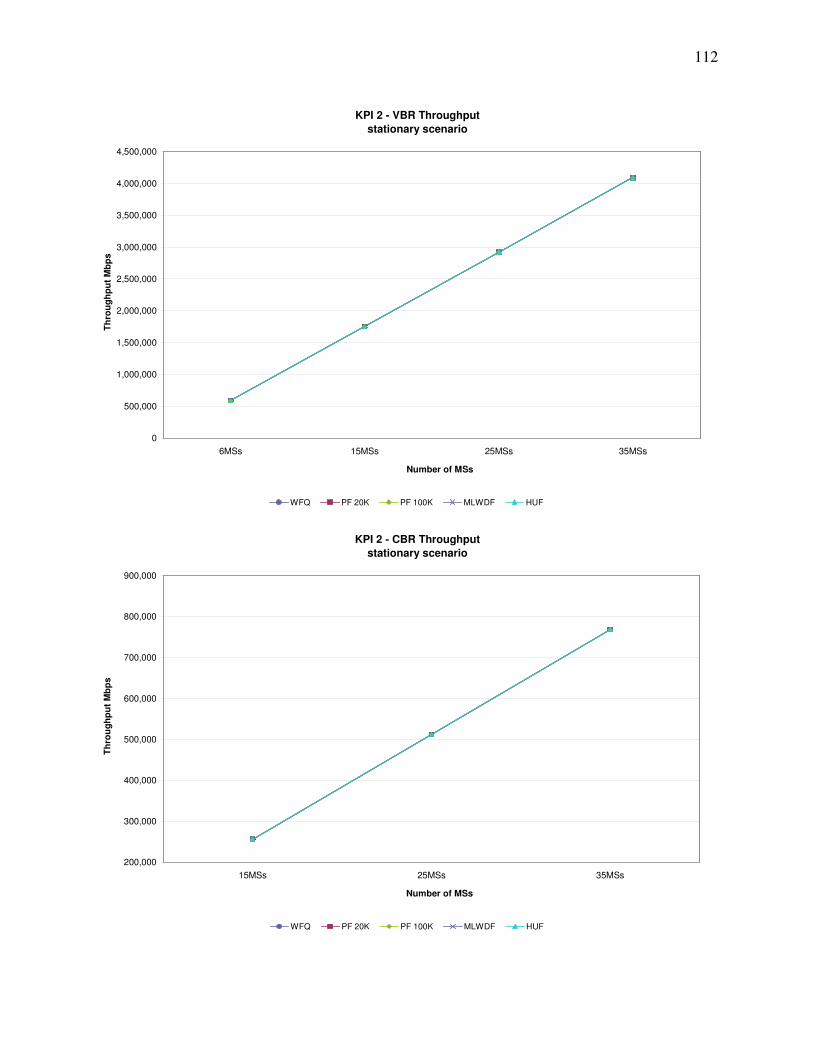
112
KPI 2 - VBR Throughput
stationary scenario
0
500,000
1,000,000
1,500,000
2,000,000
2,500,000
3,000,000
3,500,000
4,000,000
4,500,000
6MSs 15MSs 25MSs 35MSs
Number of MSs
Th
rou
gh
pu
t M
bp
s
WFQ PF 20K PF 100K MLWDF HUF
KPI 2 - CBR Throughput
stationary scenario
200,000
300,000
400,000
500,000
600,000
700,000
800,000
900,000
15MSs 25MSs 35MSs
Number of MSs
Th
rou
gh
pu
t M
bp
s
WFQ PF 20K PF 100K MLWDF HUF

113
KPI 2 - VBR Throughput
mobility scenario
0
500,000
1,000,000
1,500,000
2,000,000
2,500,000
3,000,000
3,500,000
4,000,000
6MSs 15MSs 25MSs 35MSs
Number of MSs
Th
rou
gh
pu
t M
bp
s
WFQ PF 20K PF 100K MLWDF HUF
KPI 2 - CBR Throughput
mobility scenario
200,000
300,000
400,000
500,000
600,000
700,000
800,000
15MSs 25MSs 35MSs
Number of MSs
Th
rou
gh
pu
t M
bp
s
WFQ PF 20K PF 100K MLWDF HUF
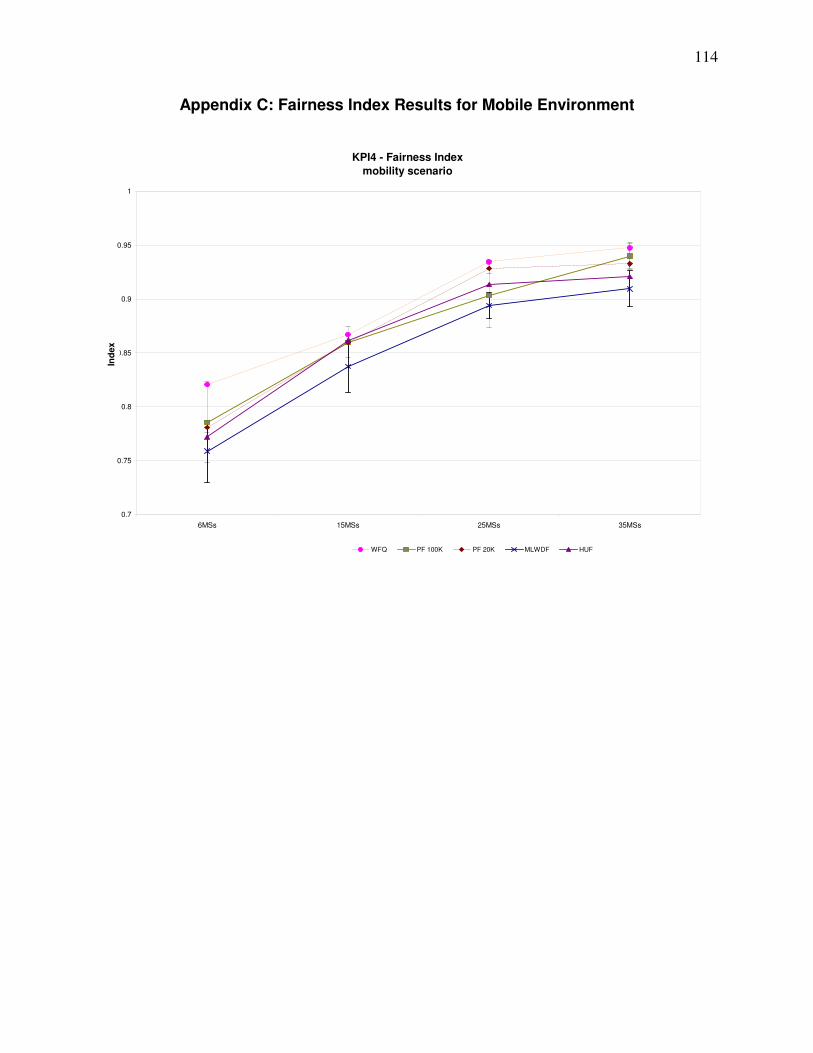
114
Appendix C: Fairness Index Results for Mobile Environment
KPI4 - Fairness Index
mobility scenario
0.7
0.75
0.8
0.85
0.9
0.95
1
6MSs 15MSs 25MSs 35MSs
Ind
ex
WFQ PF 100K PF 20K MLWDF HUF

115
Appendix D: Delay Results for Mobile Environment
KPI5 - delay (CBR)
mobility scenario
0
2
4
6
8
10
12
14
16
15MSs 25MSs 35MSs
de
lay
(m
s)
WFQ PF20K PF100K MLWDF HUF
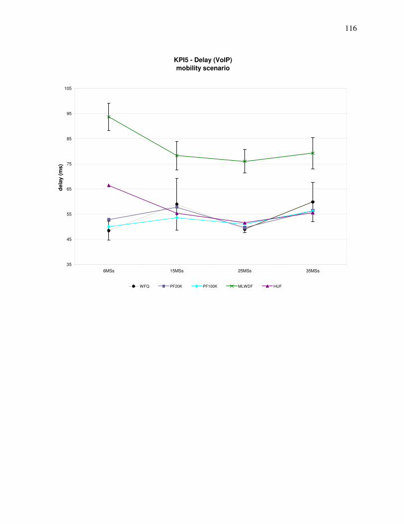
116
KPI5 - Delay (VoIP)
mobility scenario
35
45
55
65
75
85
95
105
6MSs 15MSs 25MSs 35MSs
de
lay
(m
s)
WFQ PF20K PF100K MLWDF HUF