1

McGraw-Hill/Irwin Copyright © 2007 by The McGraw-Hill Companies, Inc. All rights reserved.

16

Scheduling

16-2

Learning Objectives

Explain what scheduling involves and the

importance of good scheduling.

Discuss scheduling needs in high-volume

and intermediate-volume systems.

Discuss scheduling needs in job shops.

16-3

Learning Objectives

Use and interpret Gantt charts, and use the

assignment method for loading.

Discuss and give examples of commonly

used priority rules.

Describe some of the unique problems

encountered in service systems, and

describe some of the approaches used for

scheduling service systems.

16-4

Scheduling: Establishing the timing of

the use of equipment, facilities and

human activities in an organization

Effective scheduling can yield

Cost savings

Increases in productivity

Scheduling

2

16-5

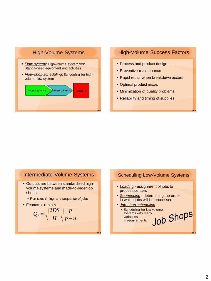
High-Volume Systems

Flow system: High-volume system with

Standardized equipment and activities

Flow-shop scheduling: Scheduling for high-

volume flow system

Work Center #1 Work Center #2 Output

16-7

High-Volume Success Factors

Process and product design

Preventive maintenance

Rapid repair when breakdown occurs

Optimal product mixes

Minimization of quality problems

Reliability and timing of supplies

16-8

Intermediate-Volume Systems

Outputs are between standardized high-

volume systems and made-to-order job

shops

Run size, timing, and sequence of jobs

Economic run size:

QDS

H

p

p u0

2

16-9

Scheduling Low-Volume Systems

Loading - assignment of jobs to process centers

Sequencing - determining the order in which jobs will be processed

Job-shop scheduling

Scheduling for low-volume systems with many variations in requirements

3

16-10

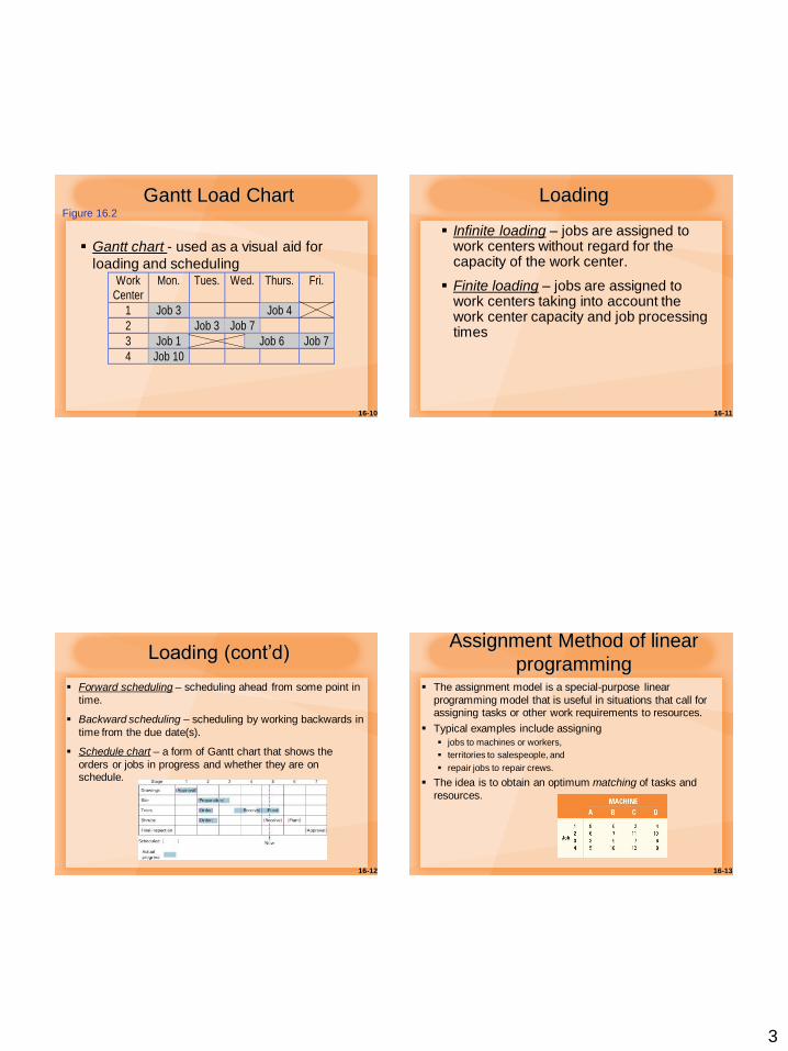
Gantt Load Chart

Gantt chart - used as a visual aid for

loading and scheduling Work

CenterMon. Tues. Wed. Thurs. Fri.

1 Job 3 Job 4

2 Job 3 Job 7

3 Job 1 Job 6 Job 7

4 Job 10

Figure 16.2

16-11

Infinite loading – jobs are assigned to work centers without regard for the capacity of the work center.

Finite loading – jobs are assigned to work centers taking into account the work center capacity and job processing times

Loading

16-12

Loading (cont’d)

Forward scheduling – scheduling ahead from some point in

time.

Backward scheduling – scheduling by working backwards in

time from the due date(s).

Schedule chart – a form of Gantt chart that shows the

orders or jobs in progress and whether they are on schedule.

Assignment Method of linear

programming The assignment model is a special-purpose linear

programming model that is useful in situations that call for assigning tasks or other work requirements to resources.

Typical examples include assigning

jobs to machines or workers,

territories to salespeople, and

repair jobs to repair crews.

The idea is to obtain an optimum matching of tasks and

resources.

16-13

4

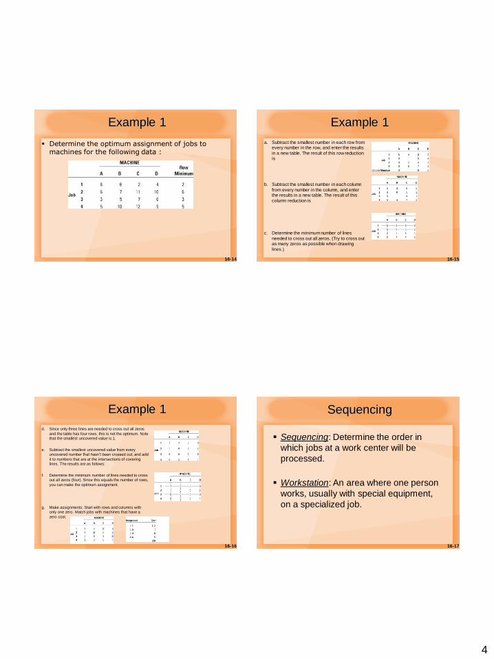
Example 1

Determine the optimum assignment of jobs to machines for the following data :

16-14

Example 1

a. Subtract the smallest number in each row from every number in the row, and enter the results

in a new table. The result of this row reduction is

b. Subtract the smallest number in each column

from every number in the column, and enter the results in a new table. The result of this

column reduction is

c. Determine the minimum number of lines

needed to cross out all zeros. (Try to cross out as many zeros as possible when drawing

lines.)

16-15

Example 1

d. Since only three lines are needed to cross out all zeros

and the table has four rows, this is not the optimum. Note that the smallest uncovered value is 1.

e. Subtract the smallest uncovered value from every uncovered number that hasn’t been crossed out, and add

it to numbers that are at the intersections of covering lines. The results are as follows:

f. Determine the minimum number of lines needed to cross out all zeros (four). Since this equals the number of rows,

you can make the optimum assignment.

g. Make assignments: Start with rows and columns with only one zero. Match jobs with machines that have a

zero cost.

16-16 16-17

Sequencing

Sequencing: Determine the order in

which jobs at a work center will be

processed.

Workstation: An area where one person

works, usually with special equipment,

on a specialized job.

5

16-18

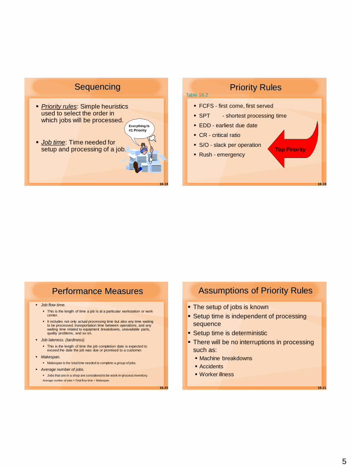
Sequencing

Priority rules: Simple heuristics used to select the order in which jobs will be processed.

Job time: Time needed for setup and processing of a job.

Everything is

#1 Priority

16-19

Priority Rules

FCFS - first come, first served

SPT - shortest processing time

EDD - earliest due date

CR - critical ratio

S/O - slack per operation

Rush - emergency Top Priority

Table 16.2

16-20

Performance Measures

Job flow time.

This is the length of time a job is at a particular workstation or work center.

It includes not only actual processing time but also any time waiting to be processed, transportation time between operations, and any waiting time related to equipment breakdowns, unavailable parts, quality problems, and so on.

Job lateness. (tardiness)

This is the length of time the job completion date is expected to exceed the date the job was due or promised to a customer.

Makespan.

Makespan is the total time needed to complete a group of jobs.

Average number of jobs.

Jobs that are in a shop are considered to be work-in-process inventory.

Average number of jobs = Total flow time ÷ Makespan

16-21

Assumptions of Priority Rules

The setup of jobs is known

Setup time is independent of processing

sequence

Setup time is deterministic

There will be no interruptions in processing

such as:

Machine breakdowns

Accidents

Worker illness

6

16-22

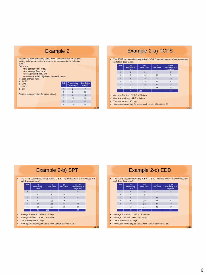
Example 2

Processing times (including setup times) and due dates for six jobs

waiting to be processed at a work center are given in the following

table.

Determine

• the sequence of jobs,

• the average flow time,

• average tardiness, and

• average number of jobs at the work center,

for each of these rules:

a. FCFS

b. SPT

c. EDD

d. CR

Assume jobs arrived in the order shown.

Job Processing Time (days)

Due Dates (days)

A 2 7

B 8 16

C 4 4

D 10 17

E 5 15

F 12 18

Example 2-a) FCFS

The FCFS sequence is simply A-B-C-D-E-F. The measures of effectiveness are

as follows (see table):

Average flow time: 120÷6 = 20 days.

Average tardiness: 54÷6 = 9 days.

The makespan is 41 days.

Average number of jobs at the work center: 120÷41 = 2.93.

16-23

Job (1)

Processing Time

(2)

Flow Time

(3)

Due Dates

(2) - (3)

Days Tardy [0 if negative]

A 2 2 7 0

B 8 10 16 0

C 4 14 4 10

D 10 24 17 7

E 5 29 15 14

F 12 41 18 23

41 120 54

Example 2-b) SPT

The FCFS sequence is simply A-B-C-D-E-F. The measures of effectiveness are

as follows (see table):

Average flow time: 108÷6 = 18 days.

Average tardiness: 40÷6 = 6.67 days.

The makespan is 41 days.

Average number of jobs at the work center: 108÷41 = 2.63.

16-24

Job (1)

Processing Time

(2)

Flow Time

(3)

Due Dates

(2) - (3)

Days Tardy [0 if negative]

A 2 2 7 0

C 4 6 4 2

E 5 11 15 0

B 8 19 16 3

D 10 29 17 12

F 12 41 18 23

41 108 40

Example 2-c) EDD

The FCFS sequence is simply A-B-C-D-E-F. The measures of effectiveness are

as follows (see table):

Average flow time: 110÷6 = 18.33 days.

Average tardiness: 38÷6 = 6.33 days.

The makespan is 41 days.

Average number of jobs at the work center: 110÷41 = 2.68.

16-25

Job (1)

Processing Time

(2)

Flow Time

(3)

Due Dates

(2) - (3)

Days Tardy [0 if negative]

C 4 4 4 0

A 2 6 7 0

E 5 11 15 0

B 8 19 16 3

D 10 29 17 12

F 12 41 18 23

41 110 38

7

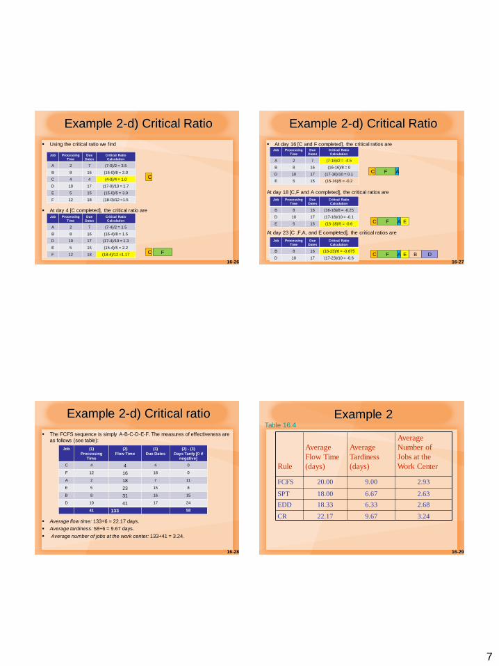
Example 2-d) Critical Ratio

Using the critical ratio we find

At day 4 [C completed], the critical ratio are

16-26

Job Processing

Time

Due

Dates

Critical Ratio

Calculation

A 2 7 (7-0)/2 = 3.5

B 8 16 (16-0)/8 = 2.0

C 4 4 (4-0)/4 = 1.0

D 10 17 (17-0)/10 = 1.7

E 5 15 (15-0)/5 = 3.0

F 12 18 (18-0)/12 =1.5

Job Processing

Time

Due

Dates

Critical Ratio

Calculation

A 2 7 (7-4)/2 = 1.5

B 8 16 (16-4)/8 = 1.5

D 10 17 (17-4)/10 = 1.3

E 5 15 (15-4)/5 = 2.2

F 12 18 (18-4)/12 =1.17

C

C F

Example 2-d) Critical Ratio

At day 16 [C and F completed], the critical ratios are

At day 18 [C,F and A completed], the critical ratios are

At day 23 [C ,F,A, and E completed], the critical ratios are

16-27

Job Processing

Time

Due

Dates

Critical Ratio

Calculation

A 2 7 (7-16)/2 = -4.5

B 8 16 (16-16)/8 = 0

D 10 17 (17-16)/10 = 0.1

E 5 15 (15-16)/5 = -0.2

Job Processing

Time

Due

Dates

Critical Ratio

Calculation

B 8 16 (16-18)/8 = -0.25

D 10 17 (17-18)/10 = -0.1

E 5 15 (15-18)/5 = -0.6

Job Processing

Time

Due

Dates

Critical Ratio

Calculation

B 8 16 (16-23)/8 = -0.875

D 10 17 (17-23)/10 = -0.6

C F A

C F A E

C F A E B D

Example 2-d) Critical ratio

The FCFS sequence is simply A-B-C-D-E-F. The measures of effectiveness are

as follows (see table):

Average flow time: 133÷6 = 22.17 days.

Average tardiness: 58÷6 = 9.67 days.

Average number of jobs at the work center: 133÷41 = 3.24.

16-28

Job (1)

Processing Time

(2)

Flow Time

(3)

Due Dates

(2) - (3)

Days Tardy [0 if negative]

C 4 4 4 0

F 12 16 18 0

A 2 18 7 11

E 5 23 15 8

B 8 31 16 15

D 10 41 17 24

41 133 58

16-29

3.24 9.67 22.17 CR

2.68 6.33 18.33 EDD

2.63 6.67 18.00 SPT

2.93 9.00 20.00 FCFS

Average

Number of

Jobs at the

Work Center

Average

Tardiness

(days)

Average

Flow Time

(days)

Rule

Example 2 Table 16.4

8

16-30

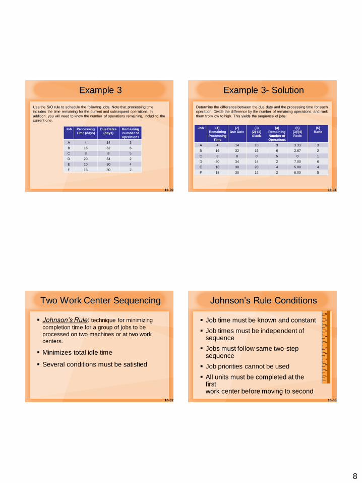
Example 3

Use the S/O rule to schedule the following jobs. Note that processing time

includes the time remaining for the current and subsequent operations. In

addition, you will need to know the number of operations remaining, including the

current one.

Job Processing Time (days)

Due Dates (days)

Remaining number of

operations

A 4 14 3

B 16 32 6

C 8 8 5

D 20 34 2

E 10 30 4

F 18 30 2

16-31

Example 3- Solution

Determine the difference between the due date and the processing time for each

operation. Divide the difference by the number of remaining operations, and rank

them from low to high. This yields the sequence of jobs:

Job (1) Remaining

Processing Time

(2) Due Date

(3) (2)-(1)

Slack

(4) Remaining

Number of Operations

(5) (3)/(4)

Ratio

(6) Rank

A 4 14 10 3 3.33 3

B 16 32 16 6 2.67 2

C 8 8 0 5 0 1

D 20 34 14 2 7.00 6

E 10 30 20 4 5.00 4

F 18 30 12 2 6.00 5

16-32

Two Work Center Sequencing

Johnson’s Rule: technique for minimizing

completion time for a group of jobs to be

processed on two machines or at two work

centers.

Minimizes total idle time

Several conditions must be satisfied

16-33

Johnson’s Rule Conditions

Job time must be known and constant

Job times must be independent of sequence

Jobs must follow same two-step sequence

Job priorities cannot be used

All units must be completed at the first work center before moving to second

9

16-34

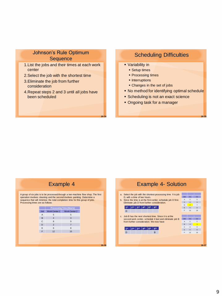
Johnson’s Rule Optimum

Sequence 1.List the jobs and their times at each work

center

2.Select the job with the shortest time

3.Eliminate the job from further

consideration

4.Repeat steps 2 and 3 until all jobs have

been scheduled

16-35

Scheduling Difficulties

Variability in

Setup times

Processing times

Interruptions

Changes in the set of jobs

No method for identifying optimal schedule

Scheduling is not an exact science

Ongoing task for a manager

16-36

Example 4

A group of six jobs is to be processed through a two-machine flow shop. The first

operation involves cleaning and the second involves painting. Determine a

sequence that will minimize the total completion time for this group of jobs.

Processing times are as follows:

Processing Time (Hours)

Job Work Center 1 Work Center 2

A 5 5

B 4 3

C 8 9

D 2 7

E 6 8

F 12 15

16-37

Example 4- Solution

a. Select the job with the shortest processing time. It is job

D, with a time of two hours.

b. Since the time is at the first center, schedule job D first.

Eliminate job D from further consideration.

c. Job B has the next shortest time. Since it is at the

second work center, schedule it last and eliminate job B

from further consideration. We now have

t

Job C1 C2

A 5 5

B 4 3

C 8 9

E 6 8

F 12 15

1st 2nd 3rd 4th 5th 6th

D

1st 2nd 3rd 4th 5th 6th

D B

t

Job C1 C2

A 5 5

C 8 9

D 2 7

E 6 8

F 12 15

10

16-38

Example 4- Solution

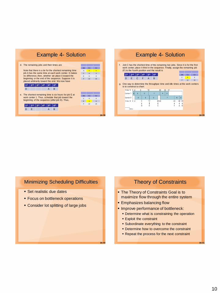
d. The remaining jobs and their times are

Note that there is a tie for the shortest remaining time:

job A has the same time at each work center. It makes

no difference, then, whether we place it toward the

beginning or the end of the sequence. Suppose it is

placed arbitrarily toward the end. We now have

e. The shortest remaining time is six hours for job E at

work center 1. Thus, schedule that job toward the

beginning of the sequence (after job D). Thus,

t

Job C1 C2

A 5 5

C 8 9

E 6 8

F 12 15

1st 2nd 3rd 4th 5th 6th

D A B

1st 2nd 3rd 4th 5th 6th

D E A B

t

Job C1 C2

C 8 9

E 6 8

F 12 15

16-39

Example 4- Solution

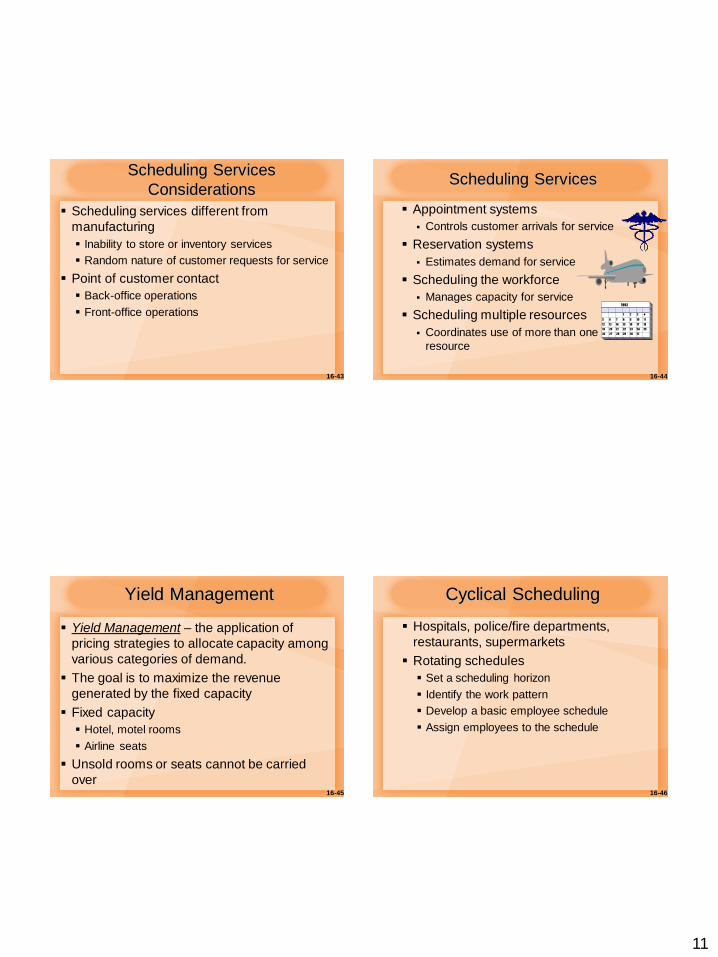
f. Job C has the shortest time of the remaining two jobs. Since it is for the first

work center, place it third in the sequence. Finally, assign the remaining job

(F) to the fourth position and the result is

g. One way to determine the throughput time and idle times at the work centers is to construct a chart:

1st 2nd 3rd 4th 5th 6th

D E C F A B

t

Job C1 C2

C 8 9

F 12 15

16-40

Minimizing Scheduling Difficulties

Set realistic due dates

Focus on bottleneck operations

Consider lot splitting of large jobs

16-41

Theory of Constraints

The Theory of Constraints Goal is to

maximize flow through the entire system

Emphasizes balancing flow

Improve performance of bottleneck:

Determine what is constraining the operation

Exploit the constraint

Subordinate everything to the constraint

Determine how to overcome the constraint

Repeat the process for the next constraint

11

16-43

Scheduling Services

Considerations

Scheduling services different from

manufacturing

Inability to store or inventory services

Random nature of customer requests for service

Point of customer contact

Back-office operations

Front-office operations

16-44

Scheduling Services

Appointment systems

Controls customer arrivals for service

Reservation systems

Estimates demand for service

Scheduling the workforce

Manages capacity for service

Scheduling multiple resources

Coordinates use of more than one

resource

16-45

Yield Management

Yield Management – the application of

pricing strategies to allocate capacity among

various categories of demand.

The goal is to maximize the revenue

generated by the fixed capacity

Fixed capacity

Hotel, motel rooms

Airline seats

Unsold rooms or seats cannot be carried

over 16-46

Cyclical Scheduling

Hospitals, police/fire departments,

restaurants, supermarkets

Rotating schedules

Set a scheduling horizon

Identify the work pattern

Develop a basic employee schedule

Assign employees to the schedule