Embed Size (px)
Citation preview

SCHEDULING PARALLEL JOBS UNDER POWER CONSTRAINTS
KunalAgrawalWashingtonUniversityinSt.Louis
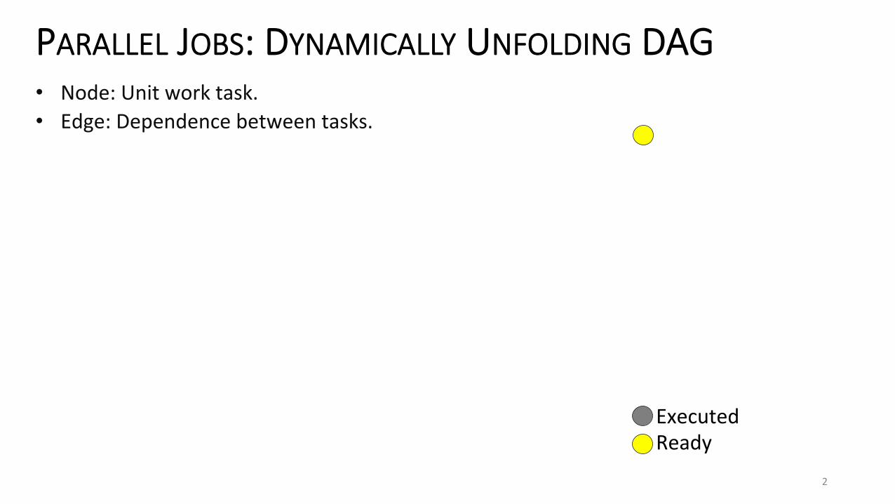
PARALLEL JOBS: DYNAMICALLY UNFOLDING DAG
ExecutedReady
2
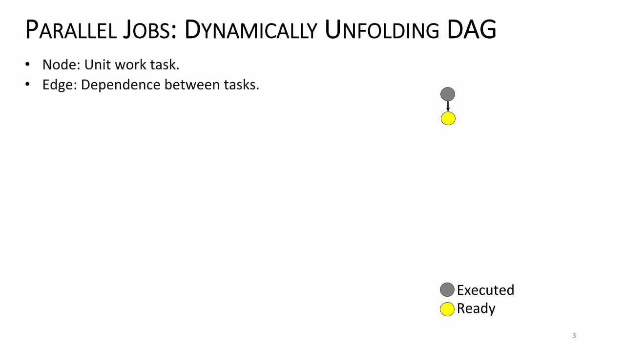
• Node:Unitworktask.• Edge:Dependencebetweentasks.
ExecutedReady
3
PARALLEL JOBS: DYNAMICALLY UNFOLDING DAG • Node:Unitworktask.• Edge:Dependencebetweentasks.
ExecutedReady
4
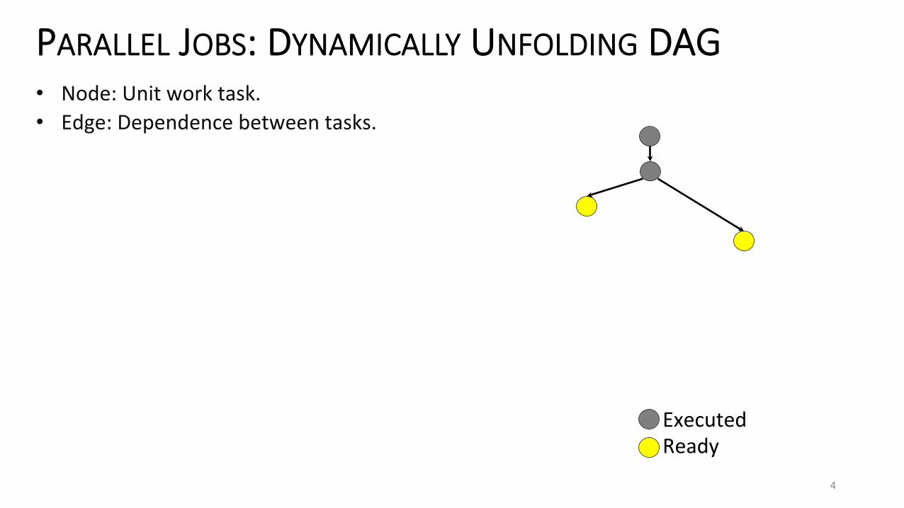
PARALLEL JOBS: DYNAMICALLY UNFOLDING DAG • Node:Unitworktask.• Edge:Dependencebetweentasks.
ExecutedReady
5
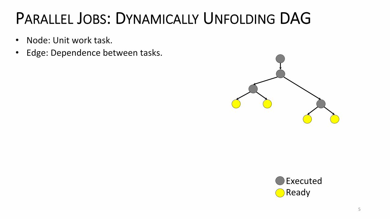
PARALLEL JOBS: DYNAMICALLY UNFOLDING DAG • Node:Unitworktask.• Edge:Dependencebetweentasks.
ExecutedReady
6
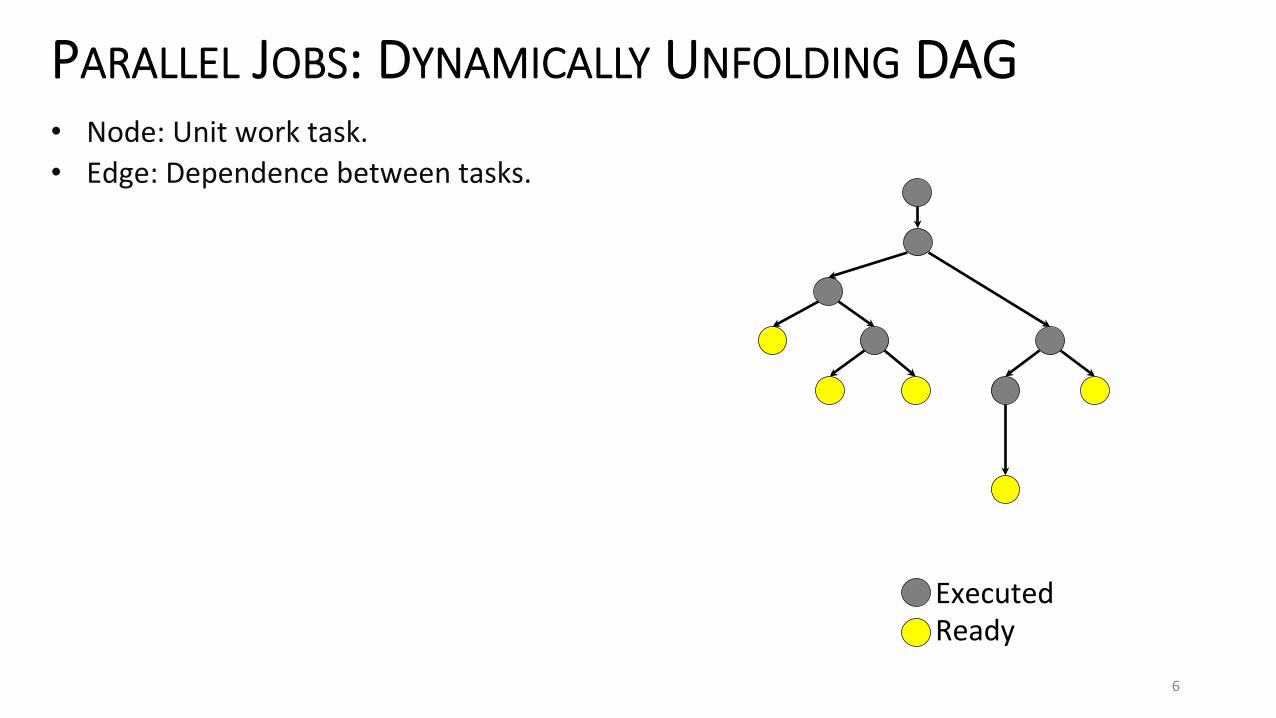
PARALLEL JOBS: DYNAMICALLY UNFOLDING DAG • Node:Unitworktask.• Edge:Dependencebetweentasks.
7
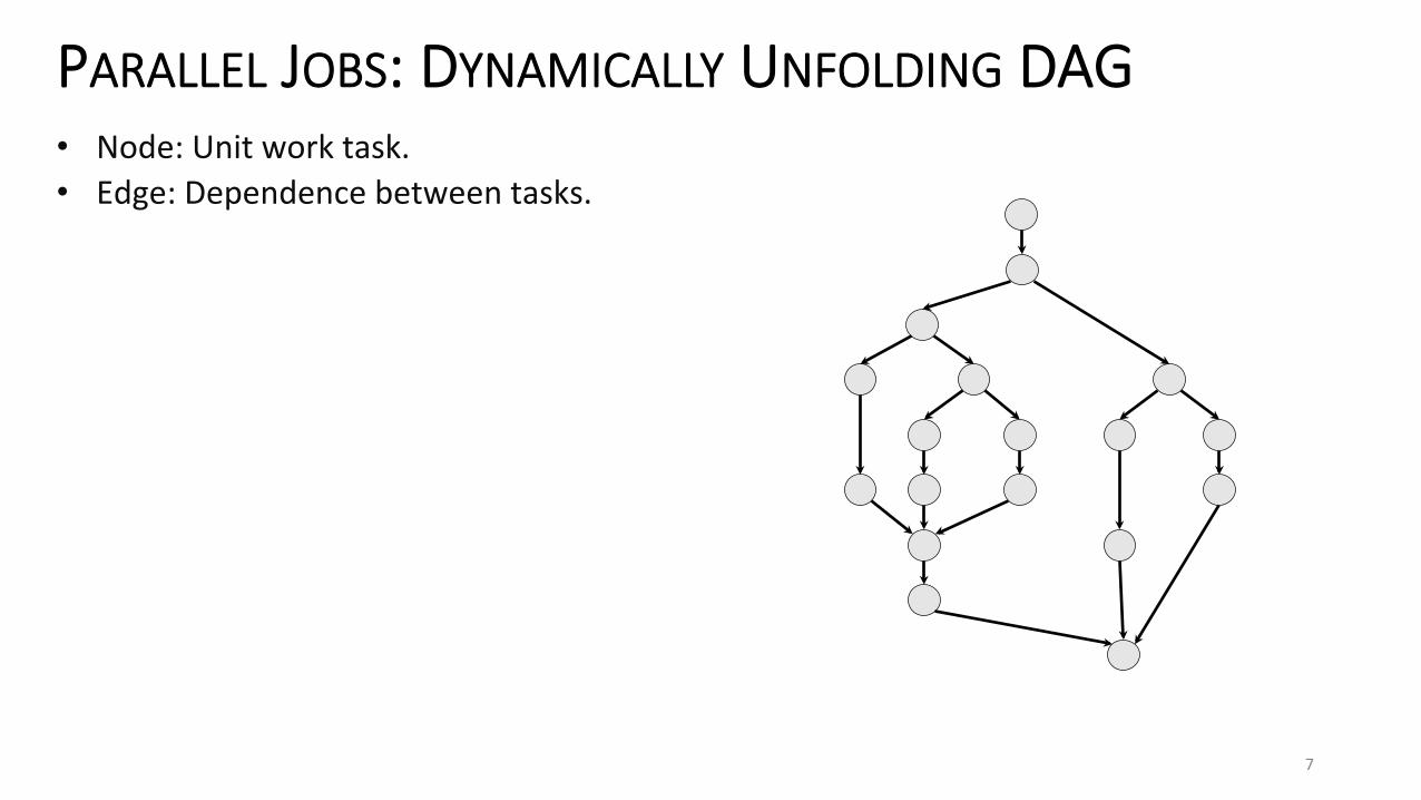
PARALLEL JOBS: DYNAMICALLY UNFOLDING DAG • Node:Unitworktask.• Edge:Dependencebetweentasks.
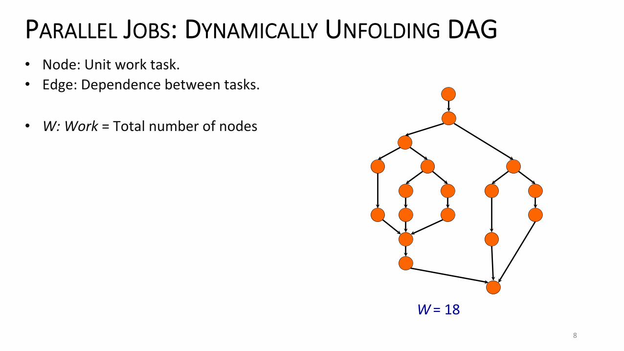
W=18
8
PARALLEL JOBS: DYNAMICALLY UNFOLDING DAG • Node:Unitworktask.• Edge:Dependencebetweentasks.
• W:Work=Totalnumberofnodes
W=18S=9
9
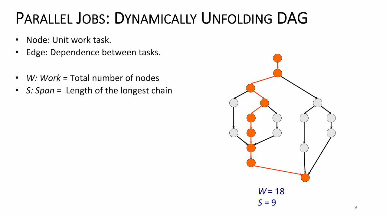
PARALLEL JOBS: DYNAMICALLY UNFOLDING DAG • Node:Unitworktask.• Edge:Dependencebetweentasks.
• W:Work=Totalnumberofnodes• S:Span=Lengthofthelongestchain
W=18S=9
10
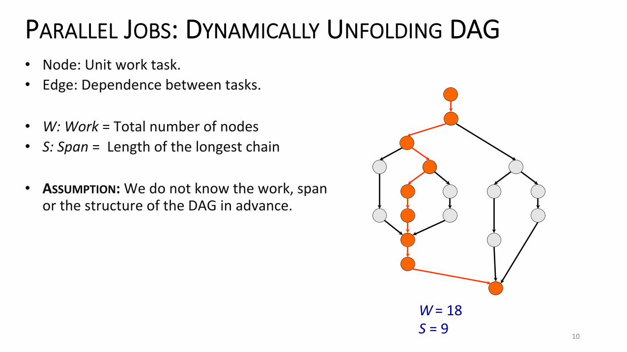
PARALLEL JOBS: DYNAMICALLY UNFOLDING DAG • Node:Unitworktask.• Edge:Dependencebetweentasks.
• W:Work=Totalnumberofnodes• S:Span=Lengthofthelongestchain
• ASSUMPTION:Wedonotknowthework,spanorthestructureoftheDAGinadvance.
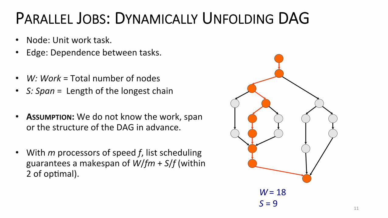
W=18S=9
11
PARALLEL JOBS: DYNAMICALLY UNFOLDING DAG • Node:Unitworktask.• Edge:Dependencebetweentasks.
• W:Work=Totalnumberofnodes• S:Span=Lengthofthelongestchain
• ASSUMPTION:Wedonotknowthework,spanorthestructureoftheDAGinadvance.
• Withmprocessorsofspeedf,listschedulingguaranteesamakespanofW/fm+S/f(within2ofopVmal).
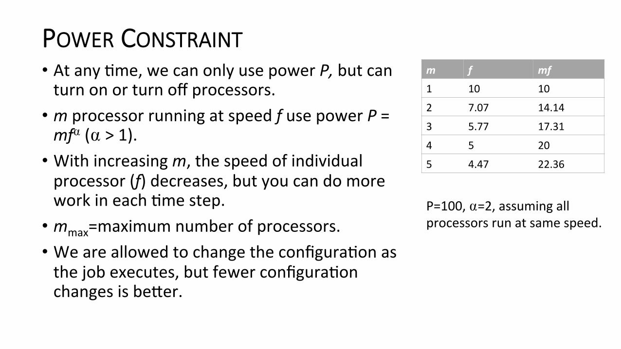
POWER CONSTRAINT • AtanyVme,wecanonlyusepowerP,butcanturnonorturnoffprocessors.• mprocessorrunningatspeedfusepowerP=mf⍺(⍺>1).• Withincreasingm,thespeedofindividualprocessor(f)decreases,butyoucandomoreworkineachVmestep.• mmax=maximumnumberofprocessors.• WeareallowedtochangetheconfiguraVonasthejobexecutes,butfewerconfiguraVonchangesisbe\er.
m f mf
1 10 10
2 7.07 14.14
3 5.77 17.31
4 5 20
5 4.47 22.36
P=100,⍺=2,assumingallprocessorsrunatsamespeed.
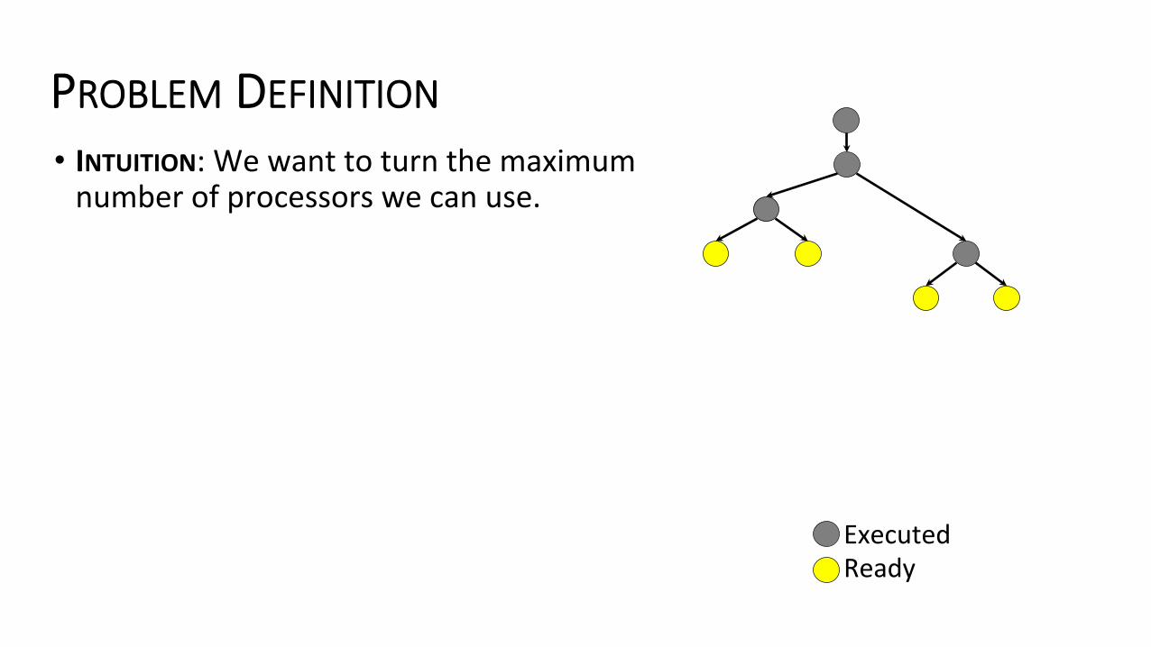
PROBLEM DEFINITION • INTUITION:Wewanttoturnthemaximumnumberofprocessorswecanuse.
ExecutedReady
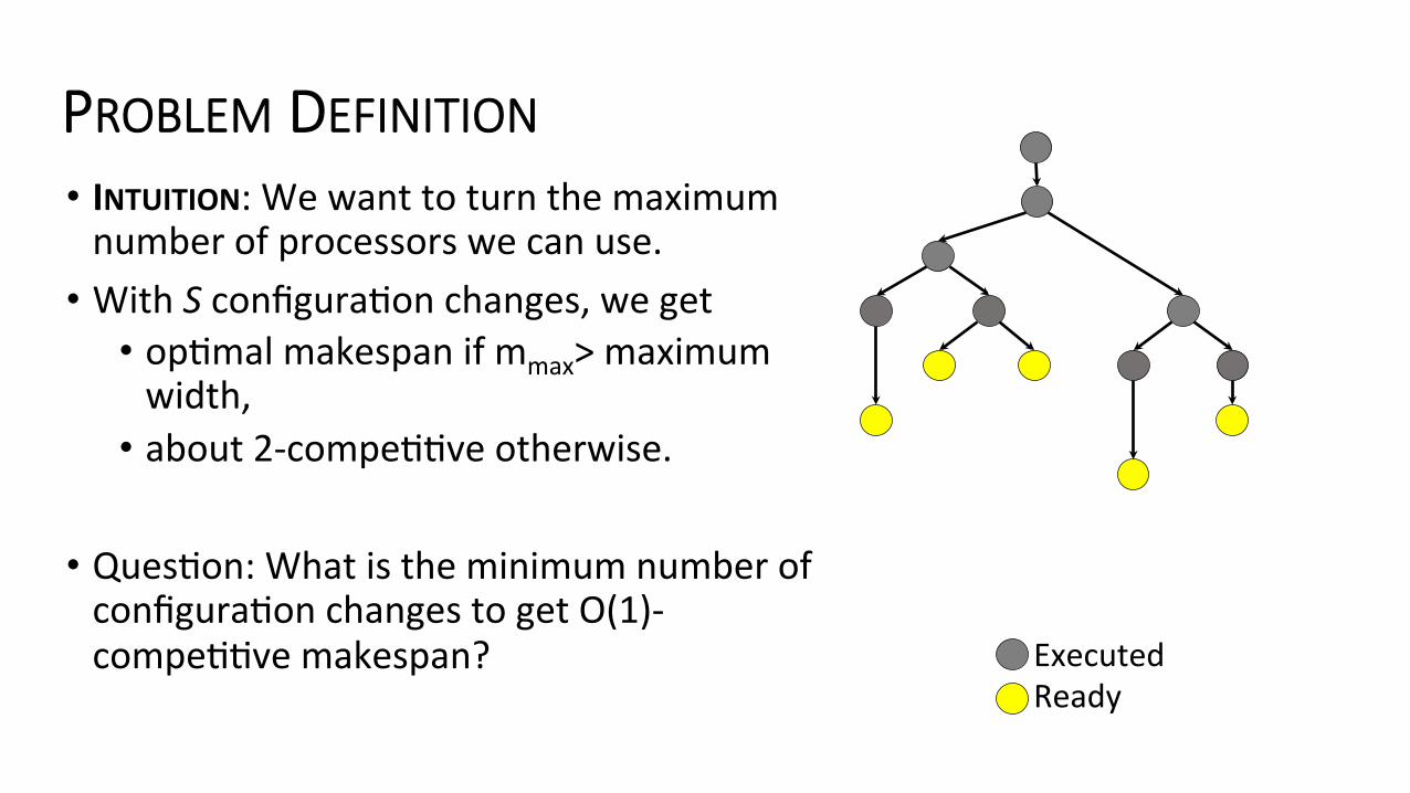
PROBLEM DEFINITION • INTUITION:Wewanttoturnthemaximumnumberofprocessorswecanuse.• WithSconfiguraVonchanges,weget• opVmalmakespanifmmax>maximumwidth,• about2-compeVVveotherwise.
• QuesVon:WhatistheminimumnumberofconfiguraVonchangestogetO(1)-compeVVvemakespan? Executed
Ready
The Home-Away-Pattern Set FeasibilityProblem
Dirk Briskorn1
1Bergische Universitat Wuppertal, Lehrstuhl fur Produktion und Logistik
D. Briskorn Home-Away-Pattern Set Feasibility 1/4
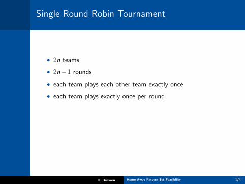
Single Round Robin Tournament
• 2n teams
• 2n−1 rounds
• each team plays each other team exactly once
• each team plays exactly once per round
1 2 3 4 5
1-2 1-3 1-4 1-5 1-65-4 2-4 3-5 4-6 5-23-6 5-6 2-6 2-3 4-3
D. Briskorn Home-Away-Pattern Set Feasibility 1/4
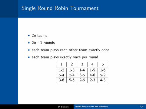
Single Round Robin Tournament
• 2n teams
• 2n−1 rounds
• each team plays each other team exactly once
• each team plays exactly once per round
1 2 3 4 5
1-2 1-3 1-4 1-5 1-65-4 2-4 3-5 4-6 5-23-6 5-6 2-6 2-3 4-3
D. Briskorn Home-Away-Pattern Set Feasibility 1/4
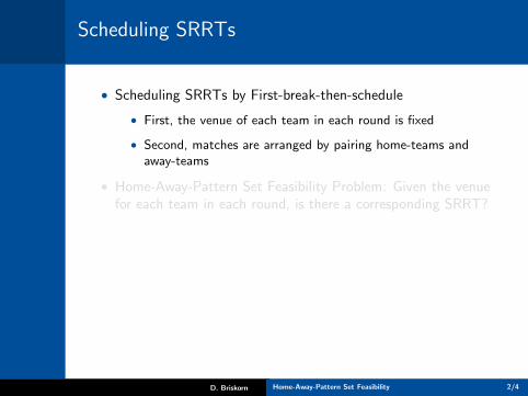
Scheduling SRRTs
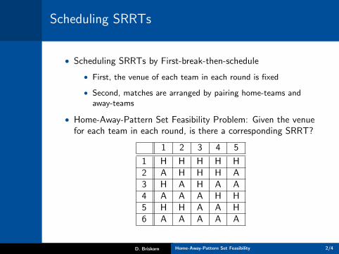
• Scheduling SRRTs by First-break-then-schedule
• First, the venue of each team in each round is fixed
• Second, matches are arranged by pairing home-teams andaway-teams
• Home-Away-Pattern Set Feasibility Problem: Given the venuefor each team in each round, is there a corresponding SRRT?
1 2 3 4 5
1 H H H H H2 A H H H A3 H A H A A4 A A A H H5 H H A A H6 A A A A A
D. Briskorn Home-Away-Pattern Set Feasibility 2/4
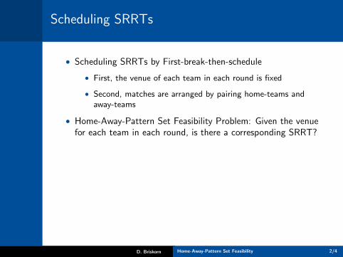
Scheduling SRRTs
• Scheduling SRRTs by First-break-then-schedule
• First, the venue of each team in each round is fixed
• Second, matches are arranged by pairing home-teams andaway-teams
• Home-Away-Pattern Set Feasibility Problem: Given the venuefor each team in each round, is there a corresponding SRRT?
1 2 3 4 5
1 H H H H H2 A H H H A3 H A H A A4 A A A H H5 H H A A H6 A A A A A
D. Briskorn Home-Away-Pattern Set Feasibility 2/4
Home-Away-Pattern Set Feasibility
• Some obvious necessary conditions
• Number of away-teams has to equal number of home-teams ineach round.
• There must not be two identical home-away patterns.
• Some less obvious ones
• Miyashiro R., Iwasaki H., Matsui T. (2003) CharacterizingFeasible Pattern Sets with a Minimum Number of Breaks. In:Burke E., De Causmaecker P. (eds) Practice and Theory ofAutomated Timetabling IV. PATAT 2002. Lecture Notes inComputer Science, vol 2740. Springer, Berlin, Heidelberg (forminimum number of breaks)
• B. (2008): Feasibility of home-away-pattern sets for round robintournaments, Operations Research Letters, Vol. 36, No. 3, pp283-284.
D. Briskorn Home-Away-Pattern Set Feasibility 3/4
Home-Away-Pattern Set Feasibility
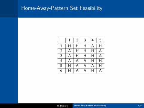
1 2 3 4 5
1 H H H A H2 A H H H A3 A H H H A4 A A A H H5 H A A A H6 H A A H A
D. Briskorn Home-Away-Pattern Set Feasibility 4/4

The Routing Open Shop Problem:Some Open Problems
Ilya Chernykh Alexandr Kononov
Sobolev Institute of MathematicsNovosibirsk, Russia
{idchern,alvenko}@math.nsc.ru
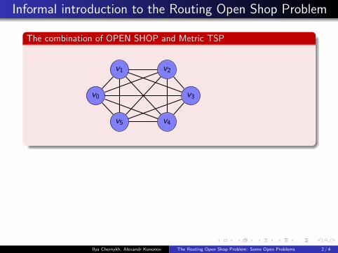
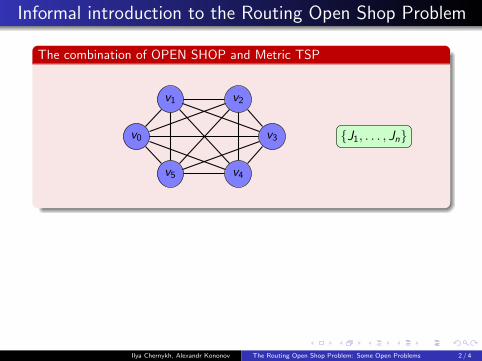
Informal introduction to the Routing Open Shop Problem
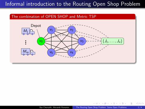
The combination of OPEN SHOP and Metric TSP
v0
v1 v2
v3
v4v5
{J1, . . . , Jn}
M1
...Mm
pji — processing time of the operation of job Jj and machine Mi ;
G = 〈V ,E 〉 — transportation network;
τkl — travel time between vk and vl ;
Ri (S) = maxk
(maxJj∈Jk
Cji (S) + τ0k
);
Rmax(S) = maxRi (S)→ minS — the makespan.
Ilya Chernykh, Alexandr Kononov The Routing Open Shop Problem: Some Open Problems 2 / 4
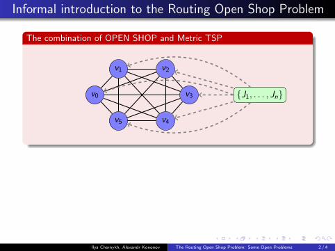
Informal introduction to the Routing Open Shop Problem
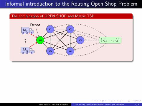
The combination of OPEN SHOP and Metric TSP
v0
v1 v2
v3
v4v5
{J1, . . . , Jn}
M1
...Mm
pji — processing time of the operation of job Jj and machine Mi ;
G = 〈V ,E 〉 — transportation network;
τkl — travel time between vk and vl ;
Ri (S) = maxk
(maxJj∈Jk
Cji (S) + τ0k
);
Rmax(S) = maxRi (S)→ minS — the makespan.
Ilya Chernykh, Alexandr Kononov The Routing Open Shop Problem: Some Open Problems 2 / 4
Informal introduction to the Routing Open Shop Problem
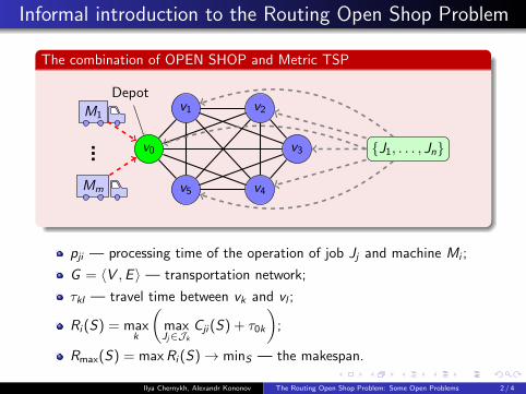
The combination of OPEN SHOP and Metric TSP
v0
v1 v2
v3
v4v5
{J1, . . . , Jn}
M1
...Mm
pji — processing time of the operation of job Jj and machine Mi ;
G = 〈V ,E 〉 — transportation network;
τkl — travel time between vk and vl ;
Ri (S) = maxk
(maxJj∈Jk
Cji (S) + τ0k
);
Rmax(S) = maxRi (S)→ minS — the makespan.
Ilya Chernykh, Alexandr Kononov The Routing Open Shop Problem: Some Open Problems 2 / 4
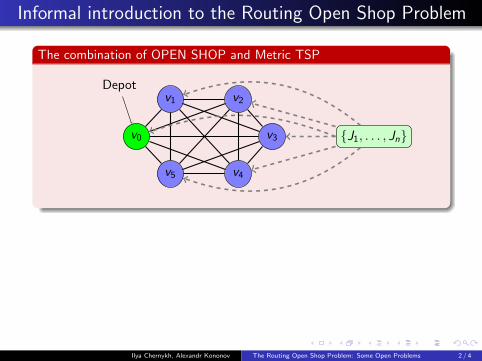
Informal introduction to the Routing Open Shop Problem
The combination of OPEN SHOP and Metric TSP
v0
v1 v2
v3
v4v5
Depot
{J1, . . . , Jn}
M1
...Mm
pji — processing time of the operation of job Jj and machine Mi ;
G = 〈V ,E 〉 — transportation network;
τkl — travel time between vk and vl ;
Ri (S) = maxk
(maxJj∈Jk
Cji (S) + τ0k
);
Rmax(S) = maxRi (S)→ minS — the makespan.
Ilya Chernykh, Alexandr Kononov The Routing Open Shop Problem: Some Open Problems 2 / 4
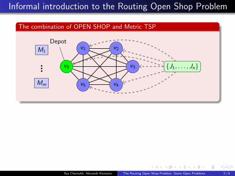
Informal introduction to the Routing Open Shop Problem
The combination of OPEN SHOP and Metric TSP
v0
v1 v2
v3
v4v5
Depot
{J1, . . . , Jn}
M1
...Mm
pji — processing time of the operation of job Jj and machine Mi ;
G = 〈V ,E 〉 — transportation network;
τkl — travel time between vk and vl ;
Ri (S) = maxk
(maxJj∈Jk
Cji (S) + τ0k
);
Rmax(S) = maxRi (S)→ minS — the makespan.
Ilya Chernykh, Alexandr Kononov The Routing Open Shop Problem: Some Open Problems 2 / 4
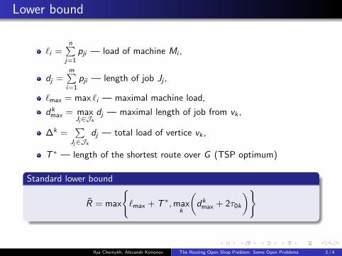
Lower bound
`i =n∑
j=1
pji — load of machine Mi ,
dj =m∑i=1
pji — length of job Jj ,
`max = max `i — maximal machine load,
dkmax = max
Jj∈Jk
dj — maximal length of job from vk ,
∆k =∑
Jj∈Jk
dj — total load of vertice vk ,
T ∗ — length of the shortest route over G (TSP optimum)
Standard lower bound
R = max
{`max + T ∗,max
k
(dkmax + 2τ0k
)}
Ilya Chernykh, Alexandr Kononov The Routing Open Shop Problem: Some Open Problems 3 / 4
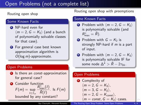
Open Problems (not a complete list)
Routing open shop
Some Known Facts
1 NP-hard even for〈m = 2,G = K2〉 (and a bunchof polynomially solvable classesfor that case).
2 For general case best knownapproximation algorithm isO(logm)-approximate.
Open Problems
1 Is there an const-approximationfor general case?
2 Consider function
F (m) = supI∈Im
R∗max(I )
R(I ). Is F (m)
bounded by any constant?
Routing open shop with preemptions
Some Known Facts
1 Problem with 〈m = 2,G = K2〉is polynomially solvable (andR∗max = R).
2 Problem with G = K2 isstrongly NP-hard if m is a partof input.
3 Problem with 〈m = 2,G = K3〉is polynomially solvable IF forsome node ∆k > R − 2τ0k .
Open Problems
1 Complexity of〈m = 2,G = K3〉,〈m = 3,G = K2〉,〈m = 2,G = Kconst〉,〈m = const,G = K2〉 cases.
Ilya Chernykh, Alexandr Kononov The Routing Open Shop Problem: Some Open Problems 4 / 4

Delayed-Clairvoyant Scheduling
Sorrachai Yingchareonthawornchai, Eric Torng Michigan State University, MI, USA
15 June 2017
The 13th Workshop on Models and Algorithms for Planning and Scheduling Problems (MAPSP 2017)
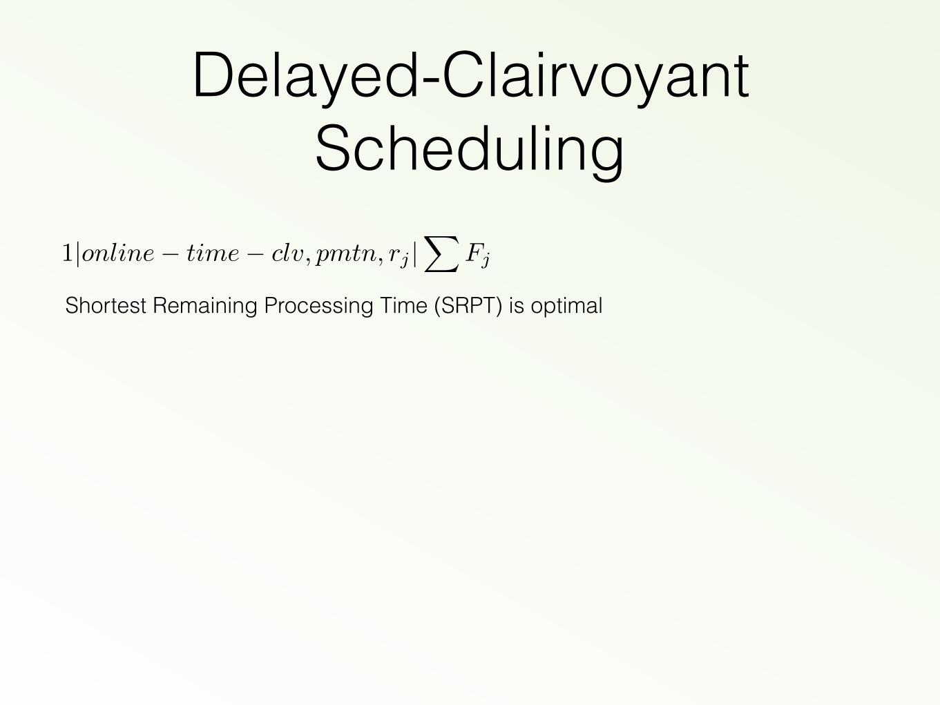
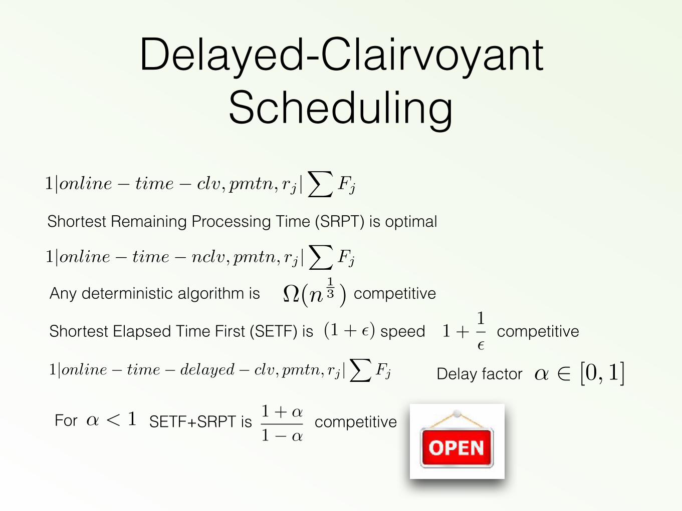
Delayed-Clairvoyant Scheduling
1|online� time� clv, pmtn, rj |X
Fj
Shortest Remaining Processing Time (SRPT) is optimal
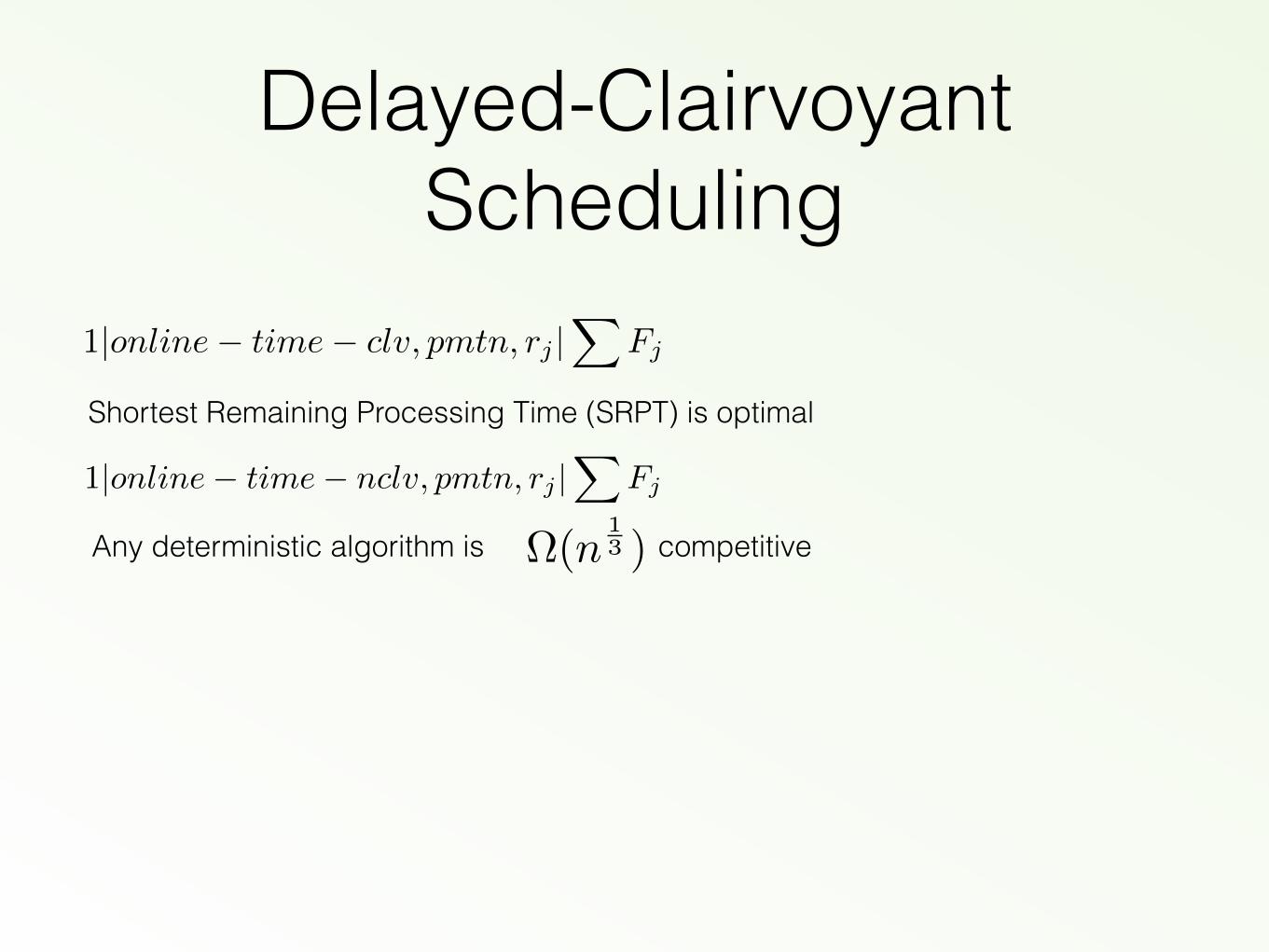
Delayed-Clairvoyant Scheduling
1|online� time� nclv, pmtn, rj |X
Fj
1|online� time� clv, pmtn, rj |X
Fj
Shortest Remaining Processing Time (SRPT) is optimal
Any deterministic algorithm is competitive ⌦(n13 )
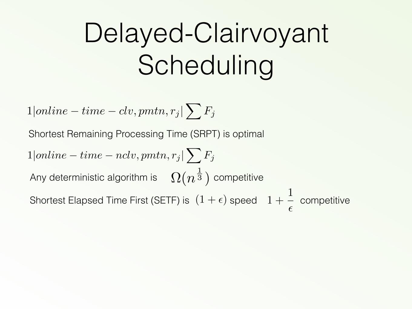
Delayed-Clairvoyant Scheduling
1|online� time� nclv, pmtn, rj |X
Fj
1|online� time� clv, pmtn, rj |X
Fj
Shortest Remaining Processing Time (SRPT) is optimal
Any deterministic algorithm is competitive ⌦(n13 )
Shortest Elapsed Time First (SETF) is speed competitive(1 + ✏) 1 +1
✏

Delayed-Clairvoyant Scheduling
1|online� time� nclv, pmtn, rj |X
Fj
1|online� time� clv, pmtn, rj |X
Fj
Shortest Remaining Processing Time (SRPT) is optimal
Any deterministic algorithm is competitive ⌦(n13 )
Shortest Elapsed Time First (SETF) is speed competitive(1 + ✏) 1 +1
✏
Delay factor ↵ 2 [0, 1]1|online� time� delayed� clv, pmtn, rj |X
Fj
Delayed-Clairvoyant Scheduling
1|online� time� nclv, pmtn, rj |X
Fj
1|online� time� clv, pmtn, rj |X
Fj
Shortest Remaining Processing Time (SRPT) is optimal
Any deterministic algorithm is competitive ⌦(n13 )
Shortest Elapsed Time First (SETF) is speed competitive(1 + ✏) 1 +1
✏
Delay factor ↵ 2 [0, 1]
1 + ↵
1� ↵SETF+SRPT is competitive ↵ < 1For
1|online� time� delayed� clv, pmtn, rj |X
Fj
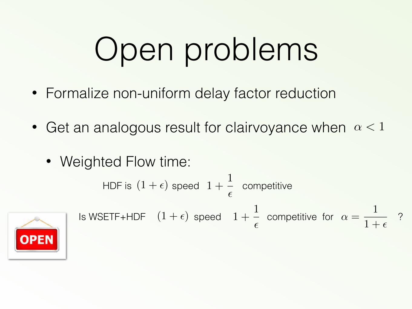
Open problems • Formalize non-uniform delay factor reduction
• Get an analogous result for clairvoyance when
• Weighted Flow time:
↵ < 1
HDF is speed competitive(1 + ✏) 1 +1
✏
Is WSETF+HDF speed competitive for ?(1 + ✏) 1 +1
✏↵ =
1
1 + ✏

A Chair’s Scheduling Problem
Samir Khuller
Research supported by NSF CCF 0937865, CCF 1217890 and Google.
University of Maryland

Whatstheproblem?
• Alumni,Companies,Deansoffice,Provost’soffice,unhappystudents,PhDstudents,facultycandidates,hiringmee?ngs,faculty,staff….
• Lotsofhourlongmee?ngs(somemul?ple)!• Mee?ngsfrom9amto6pmonly• GOAL:Maximizenumberofdaysathome!
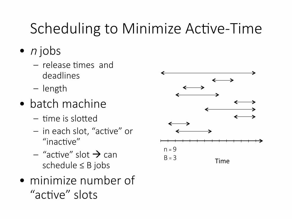
Scheduling to Minimize AcOve-Time
B = 3 n = 9
• n jobs – release Omes and
deadlines – length
• batch machine – Ome is sloWed – in each slot, “acOve” or
“inacOve” – “acOve” slot à can
schedule ≤ B jobs
• minimize number of “acOve” slots
Time
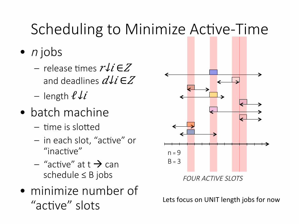
Scheduling to Minimize AcOve-Time
B = 3 n = 9
FOUR ACTIVE SLOTS
• n jobs – release Omes 𝑟↓𝑖 ∈𝑍
and deadlines 𝑑↓𝑖 ∈𝑍
– length ℓ↓𝑖 • batch machine
– Ome is sloWed – in each slot, “acOve” or
“inacOve” – “acOve” at t à can
schedule ≤ B jobs
• minimize number of “acOve” slots LetsfocusonUNITlengthjobsfornow
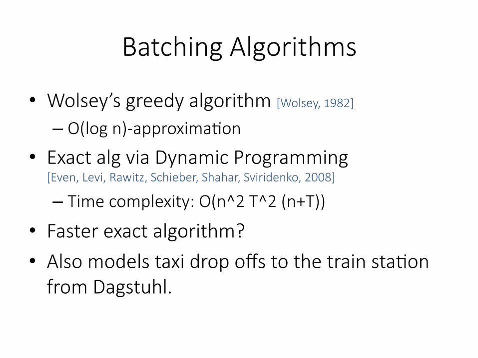
Batching Algorithms
• Wolsey’s greedy algorithm [Wolsey, 1982]
– O(log n)-approximaOon
• Exact alg via Dynamic Programming [Even, Levi, Rawitz, Schieber, Shahar, Sviridenko, 2008]
– Time complexity: O(n^2 T^2 (n+T))
• Faster exact algorithm?
• Also models taxi drop offs to the train staOon from Dagstuhl.
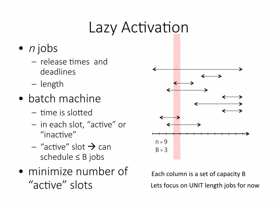
Lazy AcOvaOon
B = 3 n = 9
• n jobs – release Omes and
deadlines – length
• batch machine – Ome is sloWed – in each slot, “acOve” or
“inacOve” – “acOve” slot à can
schedule ≤ B jobs
• minimize number of “acOve” slots
EachcolumnisasetofcapacityB
LetsfocusonUNITlengthjobsfornow
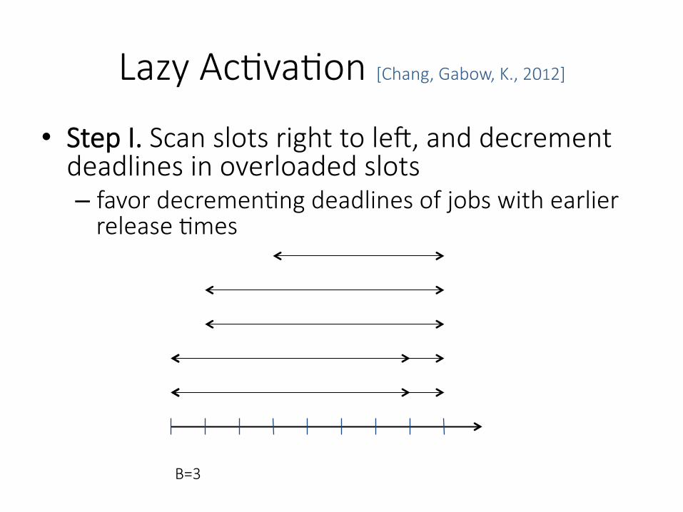
• Step I. Scan slots right to lem, and decrement deadlines in overloaded slots – favor decremenOng deadlines of jobs with earlier
release Omes
B=3
Lazy AcOvaOon [Chang, Gabow, K., 2012]
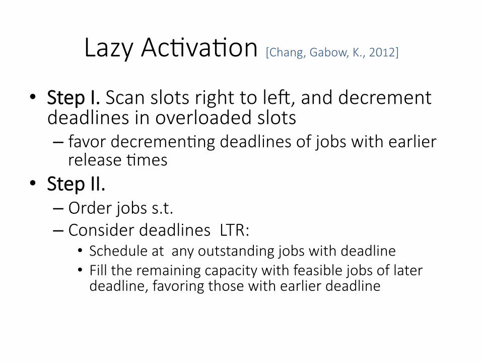
• Step I. Scan slots right to lem, and decrement deadlines in overloaded slots – favor decremenOng deadlines of jobs with earlier
release Omes • Step II. – Order jobs s.t. – Consider deadlines LTR:
• Schedule at any outstanding jobs with deadline • Fill the remaining capacity with feasible jobs of later
deadline, favoring those with earlier deadline
Lazy AcOvaOon [Chang, Gabow, K., 2012]
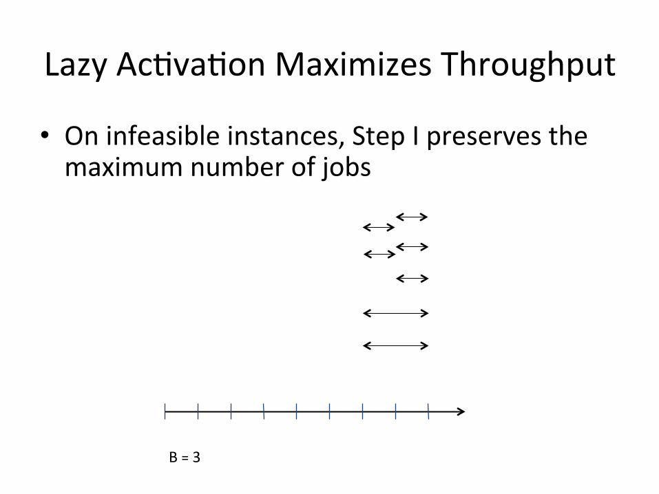
LazyAc?va?onMaximizesThroughput
• Oninfeasibleinstances,StepIpreservesthemaximumnumberofjobs
B=3
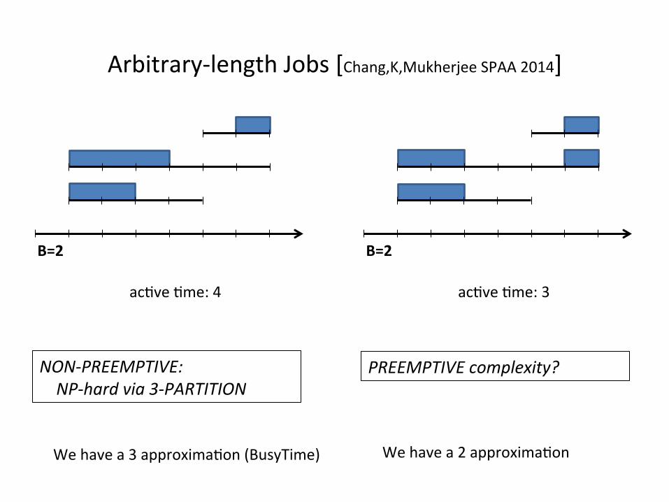
Arbitrary-lengthJobs[Chang,K,MukherjeeSPAA2014]
NON-PREEMPTIVE:NP-hardvia3-PARTITION
PREEMPTIVEcomplexity?
B=2 B=2
ac?ve?me:4 ac?ve?me:3
Wehavea2approxima?onWehavea3approxima?on(BusyTime)
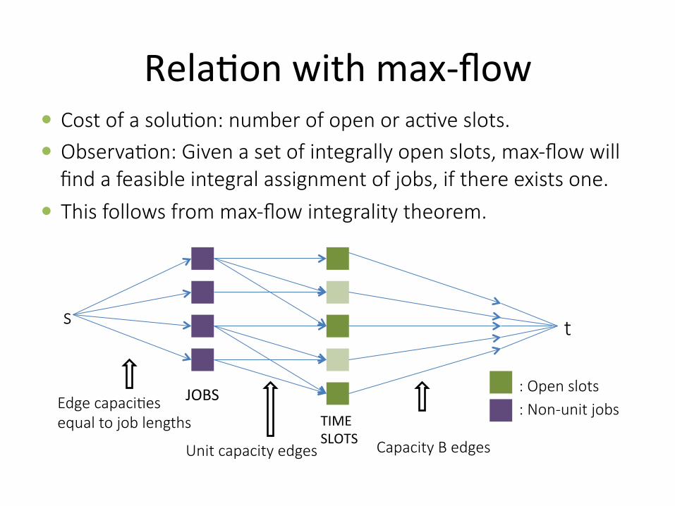
Rela?onwithmax-flow
� Cost of a soluOon: number of open or acOve slots. � ObservaOon: Given a set of integrally open slots, max-flow will
find a feasible integral assignment of jobs, if there exists one.
� This follows from max-flow integrality theorem.
t s
: Open slots : Non-unit jobs
Capacity B edges Unit capacity edges
Edge capaciOes equal to job lengths
JOBSTIMESLOTS

MinimalFeasibleSolu?ons
• Gegngjobassignmentsfromasetofac?veslots:networkflowcomputa?on
• Minimalfeasiblesolu?ons(MFS):shugngdownanyac?veslotàinfeasible
• Startfromallslotsbeingac?ve,aslongasafeasiblescheduleispossible,closeaslot
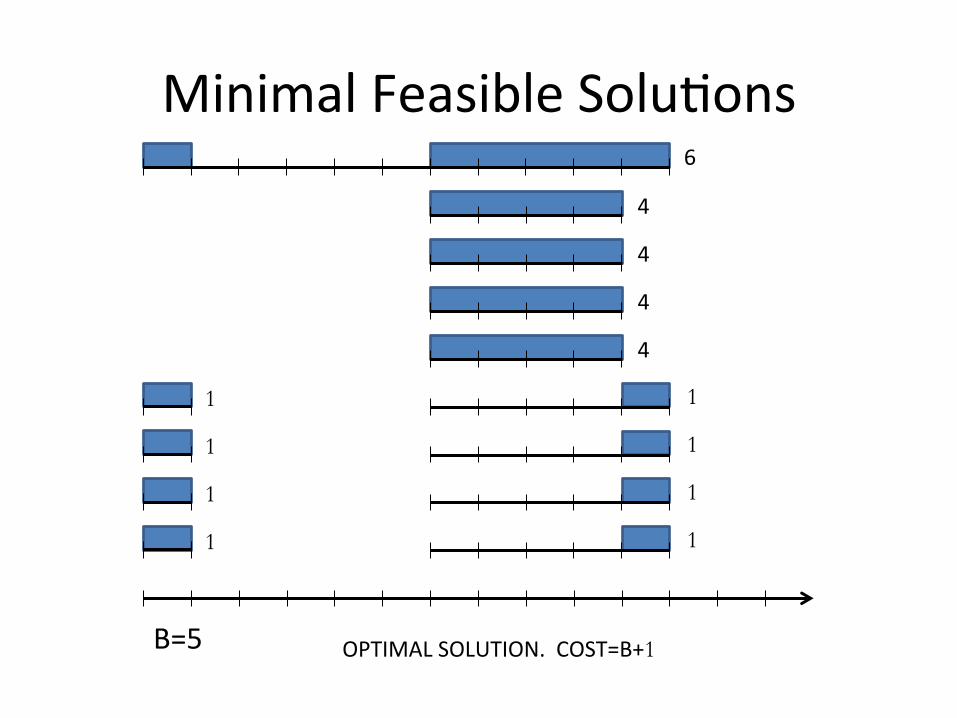
MinimalFeasibleSolu?ons6
4
1
4
4
4
B=5 OPTIMALSOLUTION.COST=B+1
1
1
1
1
1
1
1
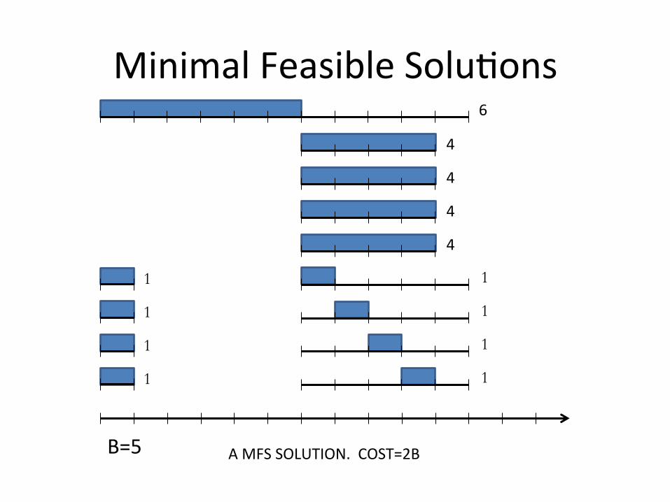
MinimalFeasibleSolu?ons6
1
B=5
1
1
1
AMFSSOLUTION.COST=2B
4
4
4
4
1
1
1
1
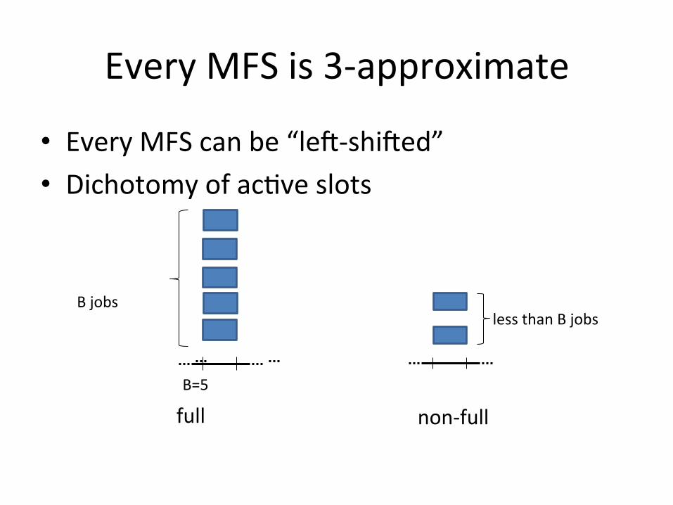
EveryMFSis3-approximate
• EveryMFScanbe“lek-shiked”• Dichotomyofac?veslots
B=5
full non-full
BjobslessthanBjobs

LProundingbasedalgorithm
],,[,0,10
,
,
,, s.t.
min
,
],[,
,
,
jjjt
t
jdrt
jt
Jjtjt
tjt
Ttt
drtxTty
Jjpx
Ttygx
TtJjyx
y
jj
…∈∀≥
∈∀≤≤
∈∀≥
∈∀≤
∈∈∀≤
∑
∑
∑
∈
∈
∈
B
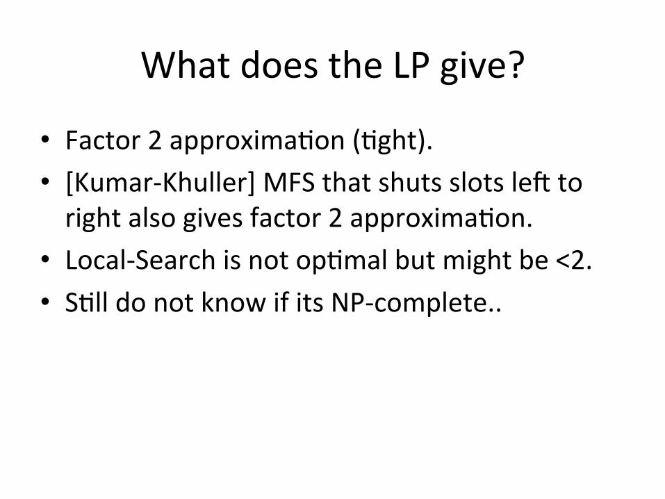
WhatdoestheLPgive?
• Factor2approxima?on(?ght).• [Kumar-Khuller]MFSthatshutsslotslektorightalsogivesfactor2approxima?on.
• Local-Searchisnotop?malbutmightbe<2.• S?lldonotknowifitsNP-complete..

Parallel Machine Scheduling with Weighted CompletionTime Objective and Online Machine Assignment
Sven Jager
Combinatorial Optimizationand Graph Algorithms
Technische Universitat Berlin
MAPSP Open Problem Session13 June 2017
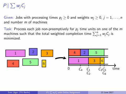
P ||∑
wjCj
Given: Jobs with processing times pj ≥ 0 and weights wj ≥ 0, j = 1, . . . , nand number m of machines
Task: Process each job non-preemptively for pj time units on one of the mmachines such that the total weighted completion time
∑nj=1 wjCj is
minimized.
1
4
2
5
3
61
4 2 5
3 6
0 timeC4 C1C2
C3C5C6
Sven Jager (TU Berlin) P||∑
wjCj with Online Assignment 13 June 2017
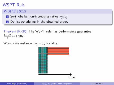
WSPT Rule
WSPT Rule
1 Sort jobs by non-increasing ratios wj/pj .
2 Do list scheduling in the obtained order.
Theorem [KK86] The WSPT rule has performance guarantee1+√
22 ≈ 1.207.
Worst case instance: wj = pj for all j .
time
Sven Jager (TU Berlin) P||∑
wjCj with Online Assignment 13 June 2017

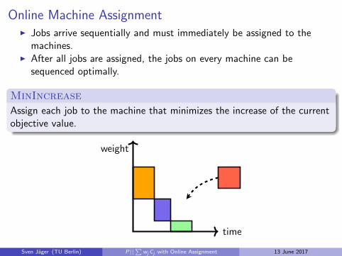
Online Machine AssignmentI Jobs arrive sequentially and must immediately be assigned to the
machines.I After all jobs are assigned, the jobs on every machine can be
sequenced optimally.
MinIncrease
Assign each job to the machine that minimizes the increase of the currentobjective value.
weight
time
Sven Jager (TU Berlin) P||∑
wjCj with Online Assignment 13 June 2017
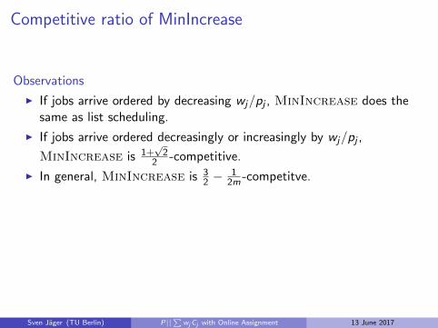
Competitive ratio of MinIncrease
Observations
I If jobs arrive ordered by decreasing wj/pj , MinIncrease does thesame as list scheduling.
I If jobs arrive ordered decreasingly or increasingly by wj/pj ,
MinIncrease is 1+√
22 -competitive.
I In general, MinIncrease is 32 −
12m -competitve.
Open Question
Is MinIncrease always 1+√
22 -competitive?
Sven Jager (TU Berlin) P||∑
wjCj with Online Assignment 13 June 2017
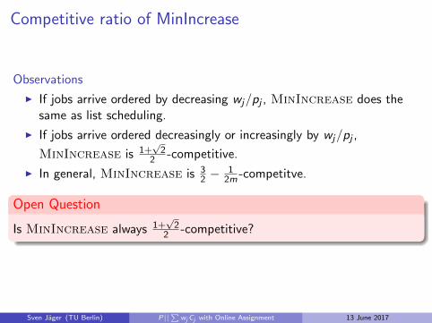
Competitive ratio of MinIncrease
Observations
I If jobs arrive ordered by decreasing wj/pj , MinIncrease does thesame as list scheduling.
I If jobs arrive ordered decreasingly or increasingly by wj/pj ,
MinIncrease is 1+√
22 -competitive.
I In general, MinIncrease is 32 −
12m -competitve.
Open Question
Is MinIncrease always 1+√
22 -competitive?
Sven Jager (TU Berlin) P||∑
wjCj with Online Assignment 13 June 2017

Appendix
Sven Jager (TU Berlin) P||∑
wjCj with Online Assignment 13 June 2017
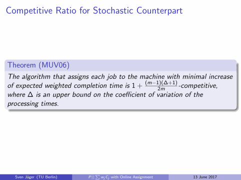
Competitive Ratio for Stochastic Counterpart
Theorem (MUV06)
The algorithm that assigns each job to the machine with minimal increaseof expected weighted completion time is 1 + (m−1)(∆+1)
2m -competitive,where ∆ is an upper bound on the coefficient of variation of theprocessing times.
Sven Jager (TU Berlin) P||∑
wjCj with Online Assignment 13 June 2017
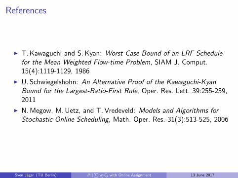
References
I T. Kawaguchi and S. Kyan: Worst Case Bound of an LRF Schedulefor the Mean Weighted Flow-time Problem, SIAM J. Comput.15(4):1119-1129, 1986
I U. Schwiegelshohn: An Alternative Proof of the Kawaguchi-KyanBound for the Largest-Ratio-First Rule, Oper. Res. Lett. 39:255-259,2011
I N. Megow, M. Uetz, and T. Vredeveld: Models and Algorithms forStochastic Online Scheduling, Math. Oper. Res. 31(3):513-525, 2006
Sven Jager (TU Berlin) P||∑
wjCj with Online Assignment 13 June 2017
Makespan minimization on parallel machines
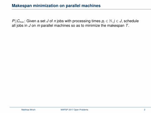
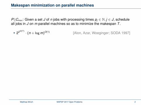
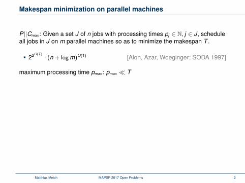
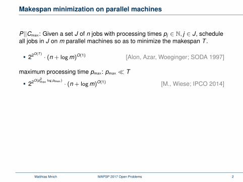
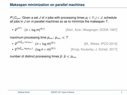
P||Cmax: Given a set J of n jobs with processing times pj ∈ N, j ∈ J, scheduleall jobs in J on m parallel machines so as to minimize the makespan T .
22O(T )
· (n + log m)O(1) [Alon, Azar, Woeginger; SODA 1997]
maximum processing time pmax: pmax � T
22O(p2max log pmax) · (n + log m)O(1) [M., Wiese; IPCO 2014]
2O(p2max log pmax) · (log n + m)O(1) [Knop, Koutecky; J. Sched. 2017]
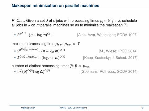
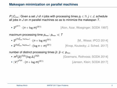
number of distinct processing times p: p � pmax
mp(p)O(p)(log ∆)O(p) [Goemans, Rothvoss; SODA 2014]
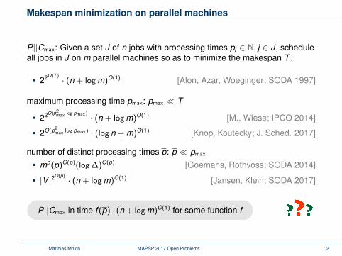
|V |2O(p)· (n + log m)O(1) [Jansen, Klein; SODA 2017]
P||Cmax in time f (p) · (n + log m)O(1) for some function f
Matthias Mnich MAPSP 2017 Open Problems 2
Makespan minimization on parallel machines
P||Cmax: Given a set J of n jobs with processing times pj ∈ N, j ∈ J, scheduleall jobs in J on m parallel machines so as to minimize the makespan T .
22O(T )
· (n + log m)O(1) [Alon, Azar, Woeginger; SODA 1997]
maximum processing time pmax: pmax � T
22O(p2max log pmax) · (n + log m)O(1) [M., Wiese; IPCO 2014]
2O(p2max log pmax) · (log n + m)O(1) [Knop, Koutecky; J. Sched. 2017]
number of distinct processing times p: p � pmax
mp(p)O(p)(log ∆)O(p) [Goemans, Rothvoss; SODA 2014]
|V |2O(p)· (n + log m)O(1) [Jansen, Klein; SODA 2017]
P||Cmax in time f (p) · (n + log m)O(1) for some function f
Matthias Mnich MAPSP 2017 Open Problems 2