Embed Size (px)
Citation preview
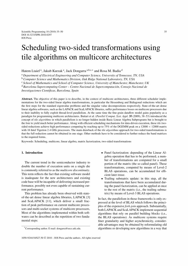
Scientific Programming 18 (2010) 35–50 35DOI 10.3233/SPR-2010-0297IOS Press
Scheduling two-sided transformations usingtile algorithms on multicore architectures
Hatem Ltaief a, Jakub Kurzak a, Jack Dongarra a,b,c,∗ and Rosa M. Badia d
a Department of Electrical Engineering and Computer Science, University of Tennessee, TN, USAb Computer Science and Mathematics Division, Oak Ridge National Laboratory, TN, USAc School of Mathematics and School of Computer Science, University of Manchester, Manchester, UKd Barcelona Supercomputing Center – Centro Nacional de Supercomputación, Consejo Nacional deInvestigaciones Cientificas, Barcelona, Spain
Abstract. The objective of this paper is to describe, in the context of multicore architectures, three different scheduler imple-mentations for the two-sided linear algebra transformations, in particular the Hessenberg and Bidiagonal reductions which arethe first steps for the standard eigenvalue problems and the singular value decompositions respectively. State-of-the-art denselinear algebra softwares, such as the LAPACK and ScaLAPACK libraries, suffer performance losses on multicore processors dueto their inability to fully exploit thread-level parallelism. At the same time the fine-grain dataflow model gains popularity as aparadigm for programming multicore architectures. Buttari et al. (Parellel Comput. Syst. Appl. 35 (2009), 38–53) introduced theconcept of tile algorithms in which parallelism is no longer hidden inside Basic Linear Algebra Subprograms but is brought tothe fore to yield much better performance. Along with efficient scheduling mechanisms for data-driven execution, these tile two-sided reductions achieve high performance computing by reaching up to 75% of the DGEMM peak on a 12000 × 12000 matrixwith 16 Intel Tigerton 2.4 GHz processors. The main drawback of the tile algorithms approach for two-sided transformations isthat the full reduction cannot be obtained in one stage. Other methods have to be considered to further reduce the band matricesto the required forms.
Keywords: Scheduling, multicore, linear algebra, matrix factorization, two-sided transformations
1. Introduction
The current trend in the semiconductor industry todouble the number of execution units on a single dieis commonly referred to as the multicore discontinuity.This term reflects the fact that existing software modelis inadequate for the new architectures and existingcode base will be incapable of delivering increased per-formance, possibly not even capable of sustaining cur-rent performance.
This problem has already been observed with state-of-the-art dense linear algebra libraries, LAPACK [3]and ScaLAPACK [11], which deliver a small frac-tion of peak performance on current multicore proces-sors and multi-socket systems of multicore processors.Most of the algorithms implemented within both soft-wares can be described as the repetition of two funda-mental steps:
*Corresponding author. E-mail: [email protected].
• Panel factorization: depending of the Linear Al-gebra operation that has to be performed, a num-ber of transformations are computed for a smallportion of the matrix (the so called panel). Thesetransformations, computed by means of Level-2BLAS operations, can be accumulated for effi-cient later reuse.
• Trailing submatrix update: in this step, all thetransformations that have been accumulated dur-ing the panel factorization, can be applied at onceto the rest of the matrix (i.e., the trailing subma-trix) by means of Level-3 BLAS operations.
In fact, the parallelism in those frameworks is only ex-pressed at the level of BLAS which follows the princi-ples of the expensive fork-join approach. Substantially,both LAPACK and ScaLAPACK implement sequentialalgorithms that rely on parallel building blocks (i.e.,the BLAS operations). As multicore systems requirefiner granularity and higher asynchronicity, consider-able advantages may be obtained by reformulating oldalgorithms or developing new algorithms in a way that
1058-9244/10/$27.50 © 2010 – IOS Press and the authors. All rights reserved
36 H. Ltaief et al. / Scheduling two-sided transformations using tile algorithms on multicore architectures
their implementation can be easily mapped on thesenew architectures.
Buttari et al. [10] introduced the concept of tile algo-rithms in which parallelism is no longer hidden insideBasic Linear Algebra Subprograms but is brought tothe fore to yield much better performance. Operationsin the standard LAPACK algorithms for some com-mon factorizations are then broken into sequences ofsmaller tasks in order to achieve finer granularity andhigher flexibility in the scheduling of tasks to cores.
This paper presents different scheduling schemesusing tile algorithms for the two-sided linear algebratransformations, in particular the Hessenberg and Bidi-agonal reductions (HRD and BRD):
• The HRD is very often used as a pre-processingstep in solving the standard eigenvalue problems(EVP) [17]:
(A − λI)x = 0,
with A ∈ Rn×n, x ∈ C
n, λ ∈ C.
The need to solve EVPs emerges from variouscomputational science disciplines including sys-tem and control theory, geophysics, molecularspectroscopy, particle physics, structure analysisand so on. The basic idea is to transform the densematrix A to an upper Hessenberg form H byapplying successive orthogonal transformationsfrom the left (Q) as well as from the right (QT) asfollows:
H = Q × A × QT,
A ∈ Rn×n, Q ∈ R
n×n, H ∈ Rn×n.
• The BRD of a general, dense matrix is very oftenused as a pre-processing step for calculating thesingular value decompositions (SVD) [17,35]:
A = XΣY T,
with A ∈ Rm×n, X ∈ R
m×m,
Σ ∈ Rm×n, Y ∈ R
n×n.
The necessity of calculating SVDs emerges fromvarious computational science disciplines, e.g., instatistics where it is related to principal compo-nent analysis, in signal processing and patternrecognition, and also in numerical weather pre-diction [12]. The basic idea is to transform thedense matrix A to an upper bidiagonal form B by
applying successive distinct orthogonal transfor-mations from the left (U ) as well as from the right(V ) as follows:
B = UT × A × V ,
A ∈ Rn×n, U ∈ R
n×n,
V ∈ Rn×n, B ∈ R
n×n.
As originally discussed in [8] for one-sided transfor-mations, the tile algorithms approach is a combinationof several concepts which are essential to match the ar-chitecture associated with the cores: (1) fine granular-ity to reach a high level of parallelism and to fit thecores’ small caches; (2) asynchronicity to prevent anyglobal barriers; (3) Block Data Layout (BDL), a highperformance data representation to perform efficientmemory access; and (4) data-driven scheduler to en-sure any enqueued tasks can immediately be processedas soon as all their data dependencies are satisfied.
By using those concepts along with efficient sched-uler implementations for data-driven execution, thesetwo-sided reductions achieve high performance com-puting. However, the main drawback of the tile algo-rithms approach for two-sided transformations is thatthe full reduction can not be obtained in one stage.Other methods have to be considered to further reducethe band matrices to the required forms. A section inthis paper will address the origin of this issue.
The remainder of this paper is organized as fol-lows: Section 2 recalls the standard HRD and BRDalgorithms. Section 3 describes the parallel HRD andBRD tile algorithms. Section 4 outlines the differentscheduling schemes. Section 5 presents performanceresults for each implementation. Section 6 gives a de-tailed overview of previous projects in this area. Fi-nally, Section 7 summarizes the results of this paperand presents the ongoing work.
2. Description of the two-sided transformations
In this section, we review the original HRD andBRD algorithms using orthogonal transformationsbased on Householder reflectors.
2.1. The standard Hessenberg reduction
The standard HRD algorithm based on Householderreflectors is written as in Algorithm 1. It takes as inputthe dense matrix A and gives as output the matrix in
H. Ltaief et al. / Scheduling two-sided transformations using tile algorithms on multicore architectures 37
Algorithm 1 Hessenberg reduction with Householderreflectors
1: for j = 1 to n − 2 do2: x = Aj+1:n,j3: vj = sign(x1)‖x‖2e1 + x4: vj = vj/‖vj ‖25: Aj+1:n,j:n = Aj+1:n,j:n − 2vj(v∗
j Aj+1:n,j:n)6: A1:n,j+1:n = A1:n,j+1:n − 2(Aj+1:n,j:nvj)v∗
j7: end for
Hessenberg form. The reflectors vj could be saved inthe lower part of A for storage purposes and used laterif necessary. The bulk of the computation is located inlines 5 and 6 in which the reflectors are applied to Afrom the left and then from the right, respectively. Fourflops are needed to update one element of the matrix.The number of operations required by the left transfor-mation (line 5) is then (the lower order terms are ne-glected):
n∑j=1
4(n − j)2 = 4
(n∑
j=1
n2 − 2n
n∑j=1
j +n∑
j=1
j2
)
� 4
(n3 − n3 +
2n3
6
)=
43n3.
Similarly, the number of operations required by theright transformation (line 6) is then:
n∑j=1
4n(n − j) = 4n
(n∑
j=1
n −n∑
j=1
j
)
� 4n
(n2 − n2
2
)= 2n3.
The total number of operations for such algorithm isfinally 4/3n3 + 2n3 = 10/3n3.
2.2. The standard Bidiagonal reduction
The standard BRD algorithm based on Householderreflectors interleaves two factorizations methods, i.e.QR (left reduction) and LQ (right reduction) decompo-sitions. The two phases are written as follows:Algorithm 2 takes as input a dense matrix A and givesas output the upper bidiagonal decomposition. The re-flectors uj and vj can be saved in the lower and upperparts of A, respectively, for storage purposes and usedlater if necessary. The bulk of the computation is lo-cated in lines 5 and 10 in which the reflectors are ap-
Algorithm 2 Bidiagonal reduction with Householderreflectors
1: for j = 1 to n do2: x = Aj:n,j3: uj = sign(x1)‖x‖2e1 + x4: uj = uj/‖uj ‖25: Aj:n,j:n = Aj:n,j:n − 2uj(u∗
jAj:n,j:n)6: if j < n then7: x = Aj,j+1:n8: vj = sign(x1)‖x‖2e1 + x9: vj = vj/‖vj ‖2
10: Aj:n,j+1:n = Aj:n,j+1:n −2(Aj:n,j+1:nvj)v∗j
11: end if12: end for
plied to A from the left and then from the right, respec-tively. Four flops are needed to update one element ofthe matrix. The left transformations (line 5) is exactlythe same than the HRD algorithm and thus, the num-ber of operations required, as explained in (1), is 4/3n3
(the lower order terms are neglected). The right trans-formation (line 10) is actually the transpose of the lefttransformation and requires the same amount of opera-tions, i.e., 4/3n3. The overall number of operations forsuch algorithm is finally 8/3n3.
2.3. The LAPACK block algorithms
The algorithms implemented in LAPACK leveragethe idea of blocking to limit the amount of bus trafficin favor of a high reuse of the data that is present in thehigher level memories which are also the fastest ones.The idea of blocking revolves around an importantproperty of Level-3 BLAS operations, the so calledsurface-to-volume property, that states that O(n3) float-ing point operations are performed on O(n2) data. Be-cause of this property, Level-3 BLAS operations canbe implemented in such a way that data movement islimited and reuse of data in the cache is maximized.Blocking algorithms consists in recasting Linear Al-gebra algorithms in a way that only a negligible partof computations is done in Level-2 BLAS operations(where no data reuse possible) while the most part isdone in Level-3 BLAS.
2.4. Limitations of the standard and block algorithms
It is obvious that Algorithms 1 and 2 are not effi-cient, especially because it is based on vector–vectorand matrix–vector operations, i.e. Level-1 and Level-2BLAS. Those operations are memory-bound on mod-
38 H. Ltaief et al. / Scheduling two-sided transformations using tile algorithms on multicore architectures
ern processors, i.e. their rate of execution is entirelydetermined by the memory latency suffered in bring-ing the operands from main memory into the floatingpoint register file.
The corresponding LAPACK block algorithms over-come some of those issues by accumulating the House-holder reflectors within the panel and then, by applyingat once to the rest of the matrix, i.e. the trailing subma-trix, which potentially make those algorithms rich inmatrix–matrix (Level-3 BLAS) operations. However,the scalability of block factorizations is limited on amulticore system when parallelism is only exploitedat the level of the BLAS routines. This approach willbe referred to as the fork-join approach since the exe-cution flow of a block factorization would show a se-quence of sequential operations (i.e., the panel factor-izations) interleaved to parallel ones (i.e., the trailingsubmatrix updates). Also, an entire column/row is re-duced at a time, which engenders a large stride accessto memory.
The whole idea is to transform these algorithms towork on a matrix split into square tiles, with clean-up regions if necessary, in the case where the size ofthe matrix does not divide evenly. All the elementswithin the tiles are contiguous in memory followingthe efficient BDL storage format and thus the accesspattern to memory is more regular. At the same time,this fine granularity greatly improves data locality andcache reuse as well as the degree of parallelism. TheHouseholder reflectors are now accumulated within thetiles during the panel factorization which decrease thelength of the stride access to memory. This algorith-mic strategy allows clever reuse of operands alreadypresent in registers, and so can run at very high rates.Those operations are indeed compute-bound, i.e. theirrate of execution principally depends on the CPU float-ing point operations per second.
The next section presents the parallel tile versions ofthese two-sided reductions.
3. The parallel band reductions
In this section, we describe the parallel implementa-tion of the HRD and BRD algorithms which reduce ageneral matrix to band form using tile algorithms.
3.1. Fast kernel descriptions
• There are four kernels to perform the tile HRDbased on Householder reflectors. Let A be a ma-
trix composed by nt × nt tiles of size b × b. LetAi,j represent the tile located at the row index iand the column index j:
– DGEQRT: this kernel performs the QR blockedfactorization of a subdiagonal tile Ak,k−1 ofthe input matrix. It produces an upper triangu-lar matrix Rk,k−1, a unit lower triangular ma-trix Vk,k−1 containing the Householder reflec-tors stored in column major format and an up-per triangular matrix Tk,k−1 as defined by theWY technique [33] for accumulating the trans-formations. Rk,k−1 and Vk,k−1 are written onthe memory area used for Ak,k−1 while an ex-tra work space is needed to store Tk,k−1. Theupper triangular matrix Rk,k−1, called refer-ence tile, is eventually used to annihilate thesubsequent tiles located below, on the samepanel.
– DTSQRT: this kernel performs the QR blockedfactorization of a matrix built by couplingthe reference tile Rk,k−1 that is producedby DGEQRT with a tile below the diagonalAi,k−1. It produces an updated Rk,k−1 factor,Vi,k−1 matrix containing the Householder re-flectors stored in column major format and thematrix Ti,k−1 resulting from accumulating thereflectors Vi,k−1.
– DLARFB: this kernel is used to apply the trans-formations computed by DGEQRT(Vk,k−1,Tk,k−1) to the tile row Ak,k:nt (left updates)and the tile column A1:nt,k (right updates).
– DSSRFB: this kernel applies the reflectorsVi,k−1 and the matrix Ti,k−1 computed byDTSQRT to two tile rows Ak,k:nt and Ai,k:nt(left updates), and two tile columns A1:nt,k andA1:nt,i (right updates).
Compared to the tile QR kernels used by Buttariet al. in [8], the right variants for DLARFB andDSSRFB have been developed. The other kernelsare exactly the same as [8]. The tile HRD algo-rithm with Householder reflectors then appears asin Algorithm 3. Figure 1 shows the HRD algo-rithm applied on a matrix with nt = 5 tiles ineach direction. The dark gray tile is the processedtile at the current step using as input dependencythe black tile, the white tiles are the tiles zeroed sofar, the bright gray tiles are those which still needto be processed and the striped tile represents thefinal data tile. For example, in Fig. 1(a), a subdi-agonal tile (in dark gray) of the first panel is re-
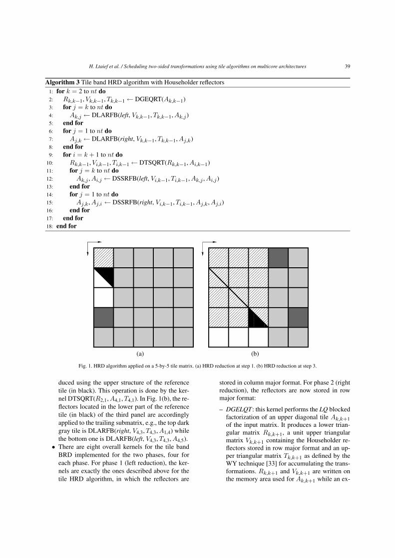
H. Ltaief et al. / Scheduling two-sided transformations using tile algorithms on multicore architectures 39
Algorithm 3 Tile band HRD algorithm with Householder reflectors1: for k = 2 to nt do2: Rk,k−1, Vk,k−1, Tk,k−1 ← DGEQRT(Ak,k−1)3: for j = k to nt do4: Ak,j ← DLARFB(left, Vk,k−1, Tk,k−1, Ak,j)5: end for6: for j = 1 to nt do7: Aj,k ← DLARFB(right, Vk,k−1, Tk,k−1, Aj,k)8: end for9: for i = k + 1 to nt do
10: Rk,k−1, Vi,k−1, Ti,k−1 ← DTSQRT(Rk,k−1, Ai,k−1)11: for j = k to nt do12: Ak,j , Ai,j ← DSSRFB(left, Vi,k−1, Ti,k−1, Ak,j , Ai,j)13: end for14: for j = 1 to nt do15: Aj,k, Aj,i ← DSSRFB(right, Vi,k−1, Ti,k−1, Aj,k, Aj,i)16: end for17: end for18: end for
(a) (b)
Fig. 1. HRD algorithm applied on a 5-by-5 tile matrix. (a) HRD reduction at step 1. (b) HRD reduction at step 3.
duced using the upper structure of the referencetile (in black). This operation is done by the ker-nel DTSQRT(R2,1, A4,1, T4,1). In Fig. 1(b), the re-flectors located in the lower part of the referencetile (in black) of the third panel are accordinglyapplied to the trailing submatrix, e.g., the top darkgray tile is DLARFB(right, V4,3, T4,3, A1,4) whilethe bottom one is DLARFB(left, V4,3, T4,3, A4,5).
• There are eight overall kernels for the tile bandBRD implemented for the two phases, four foreach phase. For phase 1 (left reduction), the ker-nels are exactly the ones described above for thetile HRD algorithm, in which the reflectors are
stored in column major format. For phase 2 (rightreduction), the reflectors are now stored in rowmajor format:
– DGELQT: this kernel performs the LQ blockedfactorization of an upper diagonal tile Ak,k+1of the input matrix. It produces a lower trian-gular matrix Rk,k+1, a unit upper triangularmatrix Vk,k+1 containing the Householder re-flectors stored in row major format and an up-per triangular matrix Tk,k+1 as defined by theWY technique [33] for accumulating the trans-formations. Rk,k+1 and Vk,k+1 are written onthe memory area used for Ak,k+1 while an ex-
40 H. Ltaief et al. / Scheduling two-sided transformations using tile algorithms on multicore architectures
Algorithm 4 Tile band BRD algorithm with Householder reflectors1: for k = 1 to nt do2: // QR Factorization3: Rk,k, Vk,k, Tk,k ← DGEQRT(Ak,k)4: for j = k + 1 to nt do5: Ak,j ← DLARFB(left, Vk,k, Tk,k, Ak,j)6: end for7: for i = k + 1 to nt do8: Rk,k, Vi,k, Ti,k ← DTSQRT(Rk,k, Ai,k)9: for j = k + 1 to nt do
10: Ak,j , Ai,j ← DSSRFB(left, Vi,k, Ti,k, Ak,j , Ai,j)11: end for12: end for13: if k < nt then14: // LQ Factorization15: Rk,k+1, Vk,k+1, Tk,k+1 ← DGELQT(Ak,k+1)16: for j = k + 1 to nt do17: Aj,k+1 ← DLARFB(right, Vk,k+1, Tk,k+1, Aj,k+1)18: end for19: for j = k + 2 to nt do20: Rk,k+1, Vk,j , Tk,j ← DTSLQT(Rk,k+1, Ak,j)21: for i = k + 1 to nt do22: Ai,k+1, Ai,j ← DSSRFB(right, Vk,i, Tk,i, Ai,k+1, Ai,j)23: end for24: end for25: end if26: end for
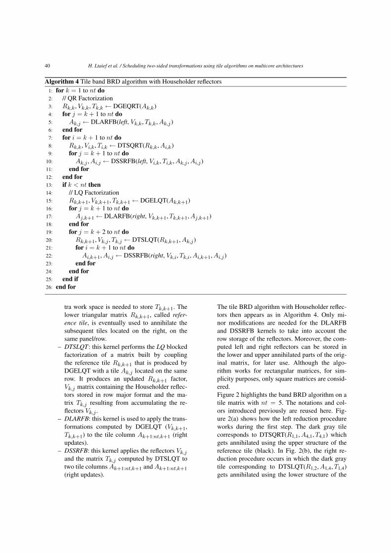
tra work space is needed to store Tk,k+1. Thelower triangular matrix Rk,k+1, called refer-ence tile, is eventually used to annihilate thesubsequent tiles located on the right, on thesame panel/row.
– DTSLQT: this kernel performs the LQ blockedfactorization of a matrix built by couplingthe reference tile Rk,k+1 that is produced byDGELQT with a tile Ak,j located on the samerow. It produces an updated Rk,k+1 factor,Vk,j matrix containing the Householder reflec-tors stored in row major format and the ma-trix Tk,j resulting from accumulating the re-flectors Vk,j .
– DLARFB: this kernel is used to apply the trans-formations computed by DGELQT (Vk,k+1,Tk,k+1) to the tile column Ak+1:nt,k+1 (rightupdates).
– DSSRFB: this kernel applies the reflectors Vk,jand the matrix Tk,j computed by DTSLQT totwo tile columns Ak+1:nt,k+1 and Ak+1:nt,k+1(right updates).
The tile BRD algorithm with Householder reflec-tors then appears as in Algorithm 4. Only mi-nor modifications are needed for the DLARFBand DSSRFB kernels to take into account therow storage of the reflectors. Moreover, the com-puted left and right reflectors can be stored inthe lower and upper annihilated parts of the orig-inal matrix, for later use. Although the algo-rithm works for rectangular matrices, for sim-plicity purposes, only square matrices are consid-ered.Figure 2 highlights the band BRD algorithm on atile matrix with nt = 5. The notations and col-ors introduced previously are reused here. Fig-ure 2(a) shows how the left reduction procedureworks during the first step. The dark gray tilecorresponds to DTSQRT(R1,1, A4,1, T4,1) whichgets annihilated using the upper structure of thereference tile (black). In Fig. 2(b), the right re-duction procedure occurs in which the dark graytile corresponding to DTSLQT(R1,2, A1,4, T1,4)gets annihilated using the lower structure of the
H. Ltaief et al. / Scheduling two-sided transformations using tile algorithms on multicore architectures 41
(a) (b)
(c) (d)
Fig. 2. BRD algorithm applied on a 5-by-5 tile matrix. (a) BRD left reduction at step 1. (b) BRD right reduction at step 1. (c) BRD left reductionat step 3. (d) BRD right reduction at step 3.
reference tile black. In Fig. 2(c), the reduc-tion is at step 3 and one of the trailing sub-matrix update operations applied on the left isrepresented by the dark gray tiles DSSRFB(left,V4,3, T4,3, A3,4, A4,4). In Fig. 2(d), one of the trail-ing submatrix update operations applied on theright is represented by the dark gray tiles in DSS-RFB(right, V3,5, T3,5, A4,4, A4,5).
All the kernels presented in this section are very richin matrix–matrix operations. By working on small tileswith BDL, the elements are contiguous in memory andthus the access pattern to memory is more regular,which makes these kernels high performing. It appearsnecessary then to efficiently schedule the kernels to gethigh performance in parallel.
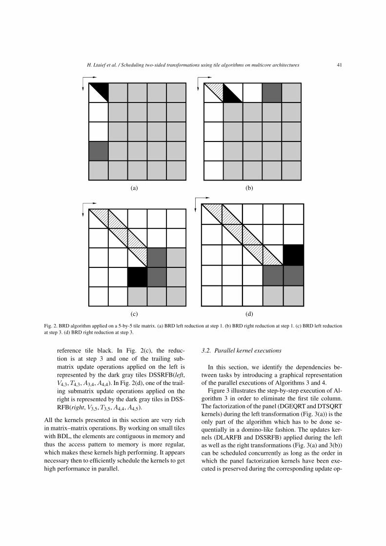
3.2. Parallel kernel executions
In this section, we identify the dependencies be-tween tasks by introducing a graphical representationof the parallel executions of Algorithms 3 and 4.
Figure 3 illustrates the step-by-step execution of Al-gorithm 3 in order to eliminate the first tile column.The factorization of the panel (DGEQRT and DTSQRTkernels) during the left transformation (Fig. 3(a)) is theonly part of the algorithm which has to be done se-quentially in a domino-like fashion. The updates ker-nels (DLARFB and DSSRFB) applied during the leftas well as the right transformations (Fig. 3(a) and 3(b))can be scheduled concurrently as long as the order inwhich the panel factorization kernels have been exe-cuted is preserved during the corresponding update op-
42 H. Ltaief et al. / Scheduling two-sided transformations using tile algorithms on multicore architectures
(a) (b)
Fig. 3. Parallel tile band HRD scheduling. (a) Left transformation. (b) Right transformation.
erations, for numerical correctness. The shape of theband Hessenberg matrix starts to appear as shown inthe bottom right matrix in Fig. 3(b).
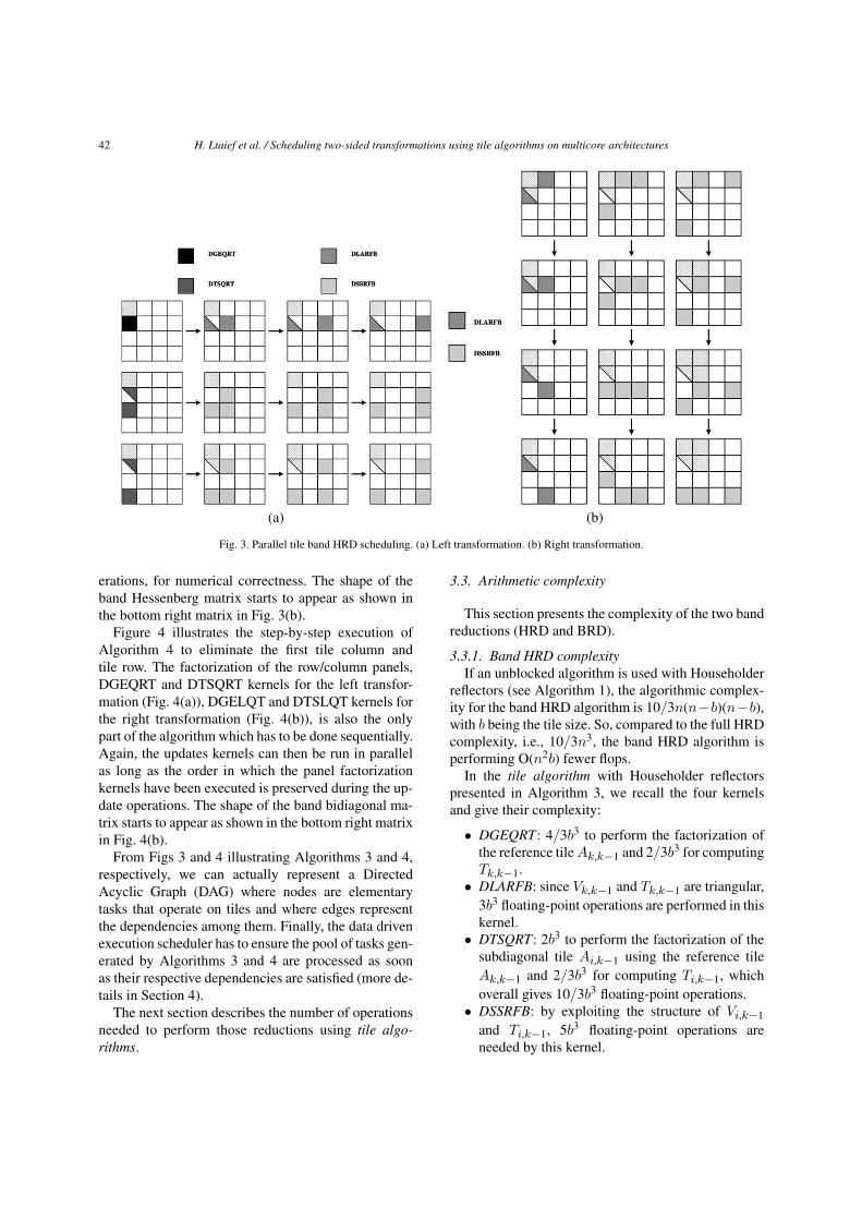
Figure 4 illustrates the step-by-step execution ofAlgorithm 4 to eliminate the first tile column andtile row. The factorization of the row/column panels,DGEQRT and DTSQRT kernels for the left transfor-mation (Fig. 4(a)), DGELQT and DTSLQT kernels forthe right transformation (Fig. 4(b)), is also the onlypart of the algorithm which has to be done sequentially.Again, the updates kernels can then be run in parallelas long as the order in which the panel factorizationkernels have been executed is preserved during the up-date operations. The shape of the band bidiagonal ma-trix starts to appear as shown in the bottom right matrixin Fig. 4(b).
From Figs 3 and 4 illustrating Algorithms 3 and 4,respectively, we can actually represent a DirectedAcyclic Graph (DAG) where nodes are elementarytasks that operate on tiles and where edges representthe dependencies among them. Finally, the data drivenexecution scheduler has to ensure the pool of tasks gen-erated by Algorithms 3 and 4 are processed as soonas their respective dependencies are satisfied (more de-tails in Section 4).
The next section describes the number of operationsneeded to perform those reductions using tile algo-rithms.
3.3. Arithmetic complexity
This section presents the complexity of the two bandreductions (HRD and BRD).
3.3.1. Band HRD complexityIf an unblocked algorithm is used with Householder
reflectors (see Algorithm 1), the algorithmic complex-ity for the band HRD algorithm is 10/3n(n − b)(n − b),with b being the tile size. So, compared to the full HRDcomplexity, i.e., 10/3n3, the band HRD algorithm isperforming O(n2b) fewer flops.
In the tile algorithm with Householder reflectorspresented in Algorithm 3, we recall the four kernelsand give their complexity:
• DGEQRT: 4/3b3 to perform the factorization ofthe reference tile Ak,k−1 and 2/3b3 for computingTk,k−1.
• DLARFB: since Vk,k−1 and Tk,k−1 are triangular,3b3 floating-point operations are performed in thiskernel.
• DTSQRT: 2b3 to perform the factorization of thesubdiagonal tile Ai,k−1 using the reference tileAk,k−1 and 2/3b3 for computing Ti,k−1, whichoverall gives 10/3b3 floating-point operations.
• DSSRFB: by exploiting the structure of Vi,k−1
and Ti,k−1, 5b3 floating-point operations areneeded by this kernel.
H. Ltaief et al. / Scheduling two-sided transformations using tile algorithms on multicore architectures 43
(a) (b)
Fig. 4. Parallel tile band BRD scheduling. (a) Left transformation. (b) Right transformation.
More details can be found in [8]. The total number offloating-point operations for the band HRD algorithmis then:
nt∑k=2
(2b3 + 3(nt − k)b3 +
103
(nt − k)b3
+ 5(nt − k)2b3 + 3b3nt
+ 5nt(nt − k + 1)b3)
� 53nt3b3 +
52nt3b3
=53n3 +
52n3
=256
n3, (1)
which is 25% higher than the unblocked algorithm forthe same reduction. Indeed, the cost of these updatingtechniques is an increase in the operation count for theband HRD algorithm. However, as suggested in [13–15], by setting up inner-blocking within the tiles duringthe panel factorizations as well as the trailing subma-trix updates (i.e., left and right), DGEQRT–DTSQRTand DLARFB–DSSRFB kernels, respectively, thoseextra flops become negligible provided s � b, with sbeing the inner-blocking size. The inner-blocking size
trades off actual memory load with those extra-flops.This blocking approach has also been described in [18,32]. To understand how this cuts the operation countof the band HRD algorithm, it is important to note thatthe DGEQRT, DLARFB and DTSQRT kernels onlyaccount for lower order terms in the total operationcount for the band HRD algorithm. It is, thus, possibleto ignore these terms and derive the operation countfor the band HRD algorithm as the sum of the costof all the DSSRFB kernels. The Ti,k−1 generated byDTSQRT and used by DSSRFB are not upper trian-gular anymore but becomes upper-triangular by blockthanks to inner-blocking. The cost of a single DSSRFBcall drops down, and by ignoring the lower order terms,it is now 4b3 + sb2. The total cost of the band HRDalgorithm with internal blocking is then:
nt∑k=2
((4b3 + sb2)(nt − k)2
+ nt(nt − k + 1)(4b3 + sb2))
� (4b3 + sb2)
(13nt3 +
12nt3
)
=(
1 +s
4b
)(43n3 + 2n3
). (2)
44 H. Ltaief et al. / Scheduling two-sided transformations using tile algorithms on multicore architectures
The operation count for the band HRD algorithm withinternal blocking is larger than that of the unblockedalgorithm only by the factor (1 + s
4b ), which is negligi-ble, provided that s � b. Note that, in the case wheres = b, the tile block Hessenberg algorithm performs25% more floating-point operations than the unblockedalgorithm, as stated before.
3.3.2. Band BRD complexitySimilarly, the same methodology is applied to com-
pute the complexity of the band BRD algorithm. Ifan unblocked algorithm is used with Householder re-flectors (see Algorithm 2), the algorithmic complexityfor the band BRD algorithm is 4/3n3 (left updates) +4/3n(n − b)(n − b) (right updates) = 4/3(n3 + n(n −b)(n − b)), with b being the tile size. So, compared tothe full BRD complexity, i.e., 8/3n3, the band BRDalgorithm is performing O(n2b) fewer flops.
The kernels involved in Algorithm 4 in the contextof tile algorithms during the left transformations arethe same than Algorithm 3. The right transformationsactually correspond to the transpose of the left trans-formations and thus, they have the same number of op-erations. The total number of floating-point operationsfor the band BRD algorithm is then:
nt∑k=2
2 ×(
2b3 + 3(nt − k)b3
+103
(nt − k)b3 + 5(nt − k)2b3)
� 2 × 53nt3b3
=103
n, (3)
which is 25% higher than the unblocked algorithm forthe same reduction. Indeed, the cost of these updat-ing techniques is an increase in the operation count forthe band BRD algorithm. Again, by setting up inner-blocking within the tiles during the panel factorizationsas well as the trailing submatrix updates (i.e., left andright), DGEQRT–DTSQRT–DLARFB–DSSRFB andDGELQT–DTSLQT–DLARFB–DSSRFB kernels, re-spectively, those extra flops become negligible pro-vided s � b, with s being the inner-blocking size.To understand how this cuts the operation count ofthe band BRD algorithm, it is important to note thatthe DGEQRT, DGELQT, DTSQRT, DTSLQT andDLARFB kernels only account for lower order terms inthe total operation count for the band BRD algorithm.
It is, thus, possible to ignore these terms and derivethe operation count for the band BRD algorithm as thesum of the cost of all the DSSRFB kernels. The Ti,k−1and Tk,j generated by DTSQRT/DTSLQT respectivelyand used by DSSRFB are not upper triangular anymorebut becomes upper-triangular by block thanks to inner-blocking. The total cost of the band BRD algorithmwith internal blocking is then:
nt∑k=2
2 × (4b3 + sb2)(nt − k)2
� 2 × (4b3 + sb2)
(13nt3
)
=(
1 +s
4b
)(83n3
). (4)
The operation count for the band BRD algorithm withinternal blocking is larger than that of the unblockedalgorithm only by the factor (1 + s
4b ), which is neg-ligible, provided that s � b. Note that, in the casewhere s = b, the band BRD algorithm performs 25%more floating-point operations than the unblocked al-gorithm, as stated above.
However, it is noteworthy to mention the high cost ofreducing the band Hessenberg/bidiagonal matrix to thefull reduced matrix. Indeed, using techniques such asbulge chasing to reduce the band matrix, especially forthe band Hessenberg, is very expensive and may dra-matically slow down the overall algorithms. Anotherapproach would be to apply the QR algorithm (non-symmetric EVP) or the Divide-and-Conquer (SVD) onthe band matrix but those strategies are sill under in-vestigations.
The next section explains the limitation origins ofthe tile algorithms concept for two-sided transforma-tions, i.e. the reduction up to band form.
3.4. Limitations of tile algorithms approach fortwo-sided transformations
The concept of tile algorithms is very suitable forone-sided methods (i.e., Cholesky, LU, QR, LQ). In-deed, the transformations are only applied to the ma-trix from one side. With the two-sided methods, theright transformation needs to preserve the reductionachieved by the left transformation. In other words,the right transformation should not destroy the zeroedstructure by creating fill-in elements. That is why, theonly way to keep intact the obtained structure is to per-
H. Ltaief et al. / Scheduling two-sided transformations using tile algorithms on multicore architectures 45
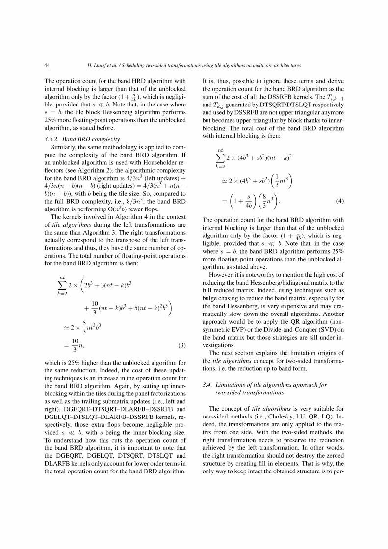
form a shift of a tile in the adequate direction. For theHRD, we shifted one tile bottom from the top-left cor-ner of the matrix. For the BRD, we decided to shift onetile right from the top-left corner of the matrix. For thelatter algorithm, we could have also performed the shiftone tile bottom from the top-left corner of the matrix.
In the following part, we present a comparison ofthree approaches for tile scheduling, i.e., a static datadriven execution scheduler, a hand-coded dynamicdata driven execution scheduler and finally, a dynamicscheduler using SMP Superscalar framework.
4. Description of the scheduling implementations
This section describes three scheduler implementa-tions: a static scheduler where the scheduling is pre-determined ahead and two dynamic schedulers wheredecisions are made at runtime.
4.1. Static scheduling
The static scheduler used here is a derivative of thescheduler used successfully in the past to scheduleCholesky and QR factorizations on the Cell proces-sor [22,24]. The static scheduler imposes a linear or-der on all the tasks in the factorization. Each threadtraverses the tasks space in this order picking a pre-determined subset of tasks for execution. In the phaseof applying transformations from the left each threadprocesses one block-column of the matrix; in the phaseof applying transformations from the right each threadprocesses one block-row of the matrix (Fig. 5). A de-pendency check is performed before executing eachtask. If dependencies are not satisfied the thread stallsuntil they are (implemented by busy waiting). Depen-dencies are tracked by a progress table, which con-tains global progress information and is replicated onall threads. Each thread calculates the task traversallocally and checks dependencies by polling the localcopy of the progress table. Due to its decentralized na-ture, the mechanism is much more scalable and of vir-tually no overhead. This technique allows for pipelinedexecution of factorizations steps, which provides sim-ilar benefits to dynamic scheduling, namely, executionof the inefficient Level 2 BLAS operations in paral-lel with the efficient Level 3 BLAS operations. Also,processing of tiles along columns and rows providesfor greater data reuse between tasks, to which the au-thors attribute the main performance advantage of thestatic scheduler. The main disadvantage of the tech-
Fig. 5. BRD Task Partitioning with eight cores on a 5 × 5 tile matrix.(The colors are visible in the online version of the article.)
nique is potentially suboptimal scheduling, i.e., stallingin situations where work is available. Another obviousweakness of the static schedule is that it cannot accom-modate dynamic operations, e.g., divide-and-conqueralgorithms.
4.2. Hand-coded dynamic scheduling
The dynamic scheduling scheme similar to [8] hasbeen extended for the two-sided orthogonal transfor-mations. A DAG is used to represent the data flowbetween the tasks/kernels. While the DAG is quiteeasy to draw for a small number of tiles, it becomesvery complex when the number of tiles increases andit is even more difficult to process than the one cre-ated by the one-sided orthogonal transformations. In-deed, the right updates impose severe constraints onthe scheduler by filling up the DAG with multiple addi-tional edges. The dynamic scheduler maintains a cen-tral progress table, which is accessed in the critical sec-tion of the code and protected with mutual exclusionprimitives (POSIX mutexes in this case). Each threadscans the table to fetch one task at a time for exe-cution. As long as there are tasks with all dependen-cies satisfied, the scheduler will provide them to therequesting threads and will allow an out-of-order exe-cution. The scheduler does not attempt to exploit datareuse between tasks though. The centralized nature of
46 H. Ltaief et al. / Scheduling two-sided transformations using tile algorithms on multicore architectures
the scheduler may inherently be non-scalable with thenumber of threads. Also, the need for scanning poten-tially large table window, in order to find work, may in-herently be non-scalable with the problem size. How-ever, this organization does not cause too much perfor-mance problems for the numbers of threads, problemsizes and task granularities investigated in this paper.
4.3. SMPSs
SMP Superscalar (SMPSs) [29,34] is a parallel pro-gramming framework developed at the Barcelona Su-percomputer Center (Centro Nacional de Supercom-putación), part of the STAR Superscalar family, whichalso includes Grid Supercalar and Cell Superscalar [5,30]. While Grid Superscalar and Cell Superscalar ad-dress parallel software development for Grid environ-ments and the Cell processor, respectively, SMP Super-scalar is aimed at “standard” (×86 and like) multicoreprocessors and symmetric multiprocessor systems. Theprogrammer is responsible for identifying paralleltasks, which have to be side-effect-free (atomic) func-tions. Additionally, the programmer needs to specifythe directionality of each parameter (input, output, in-out). If the size of a parameter is missing in the Cdeclaration (e.g., the parameter is passed by pointer),the programmer also needs to specify the size of thememory region affected by the function. However, theprogrammer is not responsible for exposing the struc-ture of the task graph. The task graph is built auto-matically, based on the information of task parametersand their directionality. The programming environmentconsists of a source-to-source compiler and a support-ing runtime library. The compiler translates C codewith pragma annotations to standard C99 code withcalls to the supporting runtime library and compiles itusing the platform native compiler (Fortran code arealso supported). At runtime the main thread createsworker threads, as many as necessary to fully utilizethe system, and starts constructing the task graph (pop-ulating its ready list). Each worker thread maintains itsown ready list and populates it while executing tasks.A thread consumes tasks from its own ready list inLIFO-order. If that list is empty, the thread consumestasks from the main ready list in FIFO-order, and ifthat list is empty, the thread steals tasks from the readylists of other threads in FIFO-order. The SMPSs sched-uler attempts to exploit locality by scheduling depen-dent tasks to the same thread, such that output data isreused immediately. Also, in order to reduce depen-
dencies, SMPSs runtime is capable of renaming data,leaving only the true dependencies.
By looking at the characteristics of the three sched-ulers, we can draw some basic conclusions. The sta-tic and the hand-coded dynamic schedulers are usingorthogonal approaches: the former emphasizes on datareuse between tasks while the latter does not stall ifwork is available. The philosophy behind the dynamicscheduler framework from SMPSs falls in the middleof the two previous schedulers because not only it pro-ceeds as soon as work is available, but also it tries toreuse data as much as possible. Another aspect whichhas to be taken into account is the coding effort. In-deed, the easy of use of SMPSs makes it very attractivefor end-users and puts it on top of the other schedulersdiscussed in this paper.
5. Experimental results
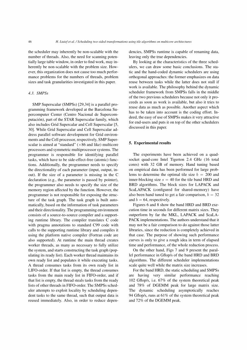
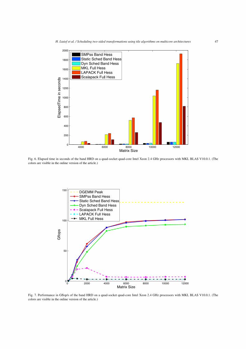
The experiments have been achieved on a quad-socket quad-core Intel Tigerton 2.4 GHz (16 totalcores) with 32 GB of memory. Hand tuning basedon empirical data has been performed for large prob-lems to determine the optimal tile size b = 200 andinner-blocking size s = 40 for the tile band HRD andBRD algorithms. The block sizes for LAPACK andScaLAPACK (configured for shared-memory) havealso been hand tuned to get a fair comparison, b = 32and b = 64, respectively.
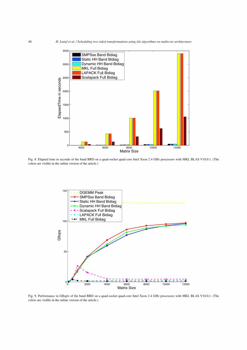
Figures 6 and 8 show the band HRD and BRD exe-cution time in seconds for different matrix sizes. Theyoutperform by far the MKL, LAPACK and ScaLA-PACK implementations. The authors understand that itmay not be a fair comparison to do against those latterlibraries, since the reduction is completely achieved inthat case. The purpose of showing such performancecurves is only to give a rough idea in term of elapsedtime and performance, of the whole reduction process.
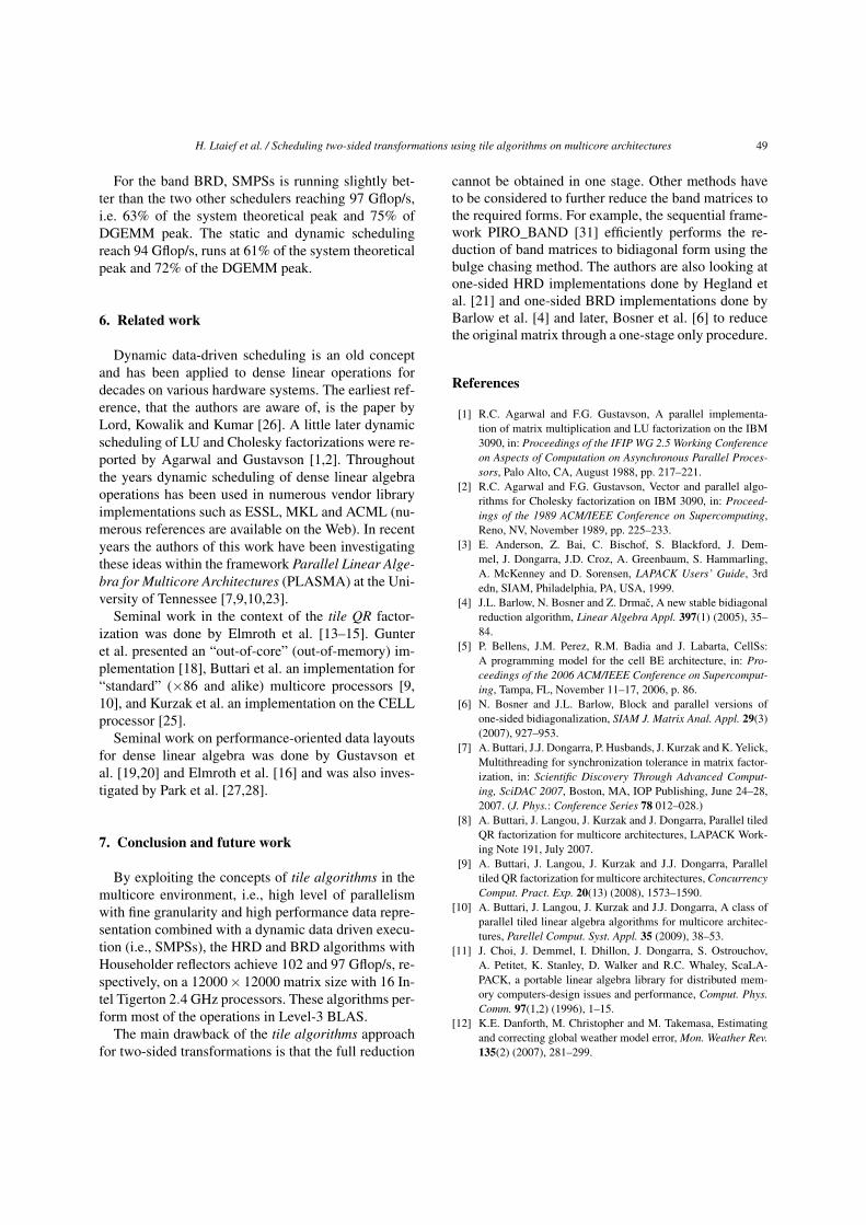
On the other hand, Figs 7 and 9 present the paral-lel performance in Gflop/s of the band HRD and BRDalgorithms. The different scheduler implementationsscale quite well while the matrix size increases.
For the band HRD, the static scheduling and SMPSsare having very similar performance reaching102 Gflop/s, i.e. 67% of the system theoretical peakand 78% of DGEMM peak for large matrix size.The dynamic scheduling asymptotically reaches94 Gflop/s, runs at 61% of the system theoretical peakand 72% of the DGEMM peak.
H. Ltaief et al. / Scheduling two-sided transformations using tile algorithms on multicore architectures 47
Fig. 6. Elapsed time in seconds of the band HRD on a quad-socket quad-core Intel Xeon 2.4 GHz processors with MKL BLAS V10.0.1. (Thecolors are visible in the online version of the article.)
Fig. 7. Performance in Gflop/s of the band HRD on a quad-socket quad-core Intel Xeon 2.4 GHz processors with MKL BLAS V10.0.1. (Thecolors are visible in the online version of the article.)
48 H. Ltaief et al. / Scheduling two-sided transformations using tile algorithms on multicore architectures
Fig. 8. Elapsed time in seconds of the band BRD on a quad-socket quad-core Intel Xeon 2.4 GHz processors with MKL BLAS V10.0.1. (Thecolors are visible in the online version of the article.)
Fig. 9. Performance in Gflop/s of the band BRD on a quad-socket quad-core Intel Xeon 2.4 GHz processors with MKL BLAS V10.0.1. (Thecolors are visible in the online version of the article.)
H. Ltaief et al. / Scheduling two-sided transformations using tile algorithms on multicore architectures 49
For the band BRD, SMPSs is running slightly bet-ter than the two other schedulers reaching 97 Gflop/s,i.e. 63% of the system theoretical peak and 75% ofDGEMM peak. The static and dynamic schedulingreach 94 Gflop/s, runs at 61% of the system theoreticalpeak and 72% of the DGEMM peak.
6. Related work
Dynamic data-driven scheduling is an old conceptand has been applied to dense linear operations fordecades on various hardware systems. The earliest ref-erence, that the authors are aware of, is the paper byLord, Kowalik and Kumar [26]. A little later dynamicscheduling of LU and Cholesky factorizations were re-ported by Agarwal and Gustavson [1,2]. Throughoutthe years dynamic scheduling of dense linear algebraoperations has been used in numerous vendor libraryimplementations such as ESSL, MKL and ACML (nu-merous references are available on the Web). In recentyears the authors of this work have been investigatingthese ideas within the framework Parallel Linear Alge-bra for Multicore Architectures (PLASMA) at the Uni-versity of Tennessee [7,9,10,23].
Seminal work in the context of the tile QR factor-ization was done by Elmroth et al. [13–15]. Gunteret al. presented an “out-of-core” (out-of-memory) im-plementation [18], Buttari et al. an implementation for“standard” (×86 and alike) multicore processors [9,10], and Kurzak et al. an implementation on the CELLprocessor [25].
Seminal work on performance-oriented data layoutsfor dense linear algebra was done by Gustavson etal. [19,20] and Elmroth et al. [16] and was also inves-tigated by Park et al. [27,28].
7. Conclusion and future work
By exploiting the concepts of tile algorithms in themulticore environment, i.e., high level of parallelismwith fine granularity and high performance data repre-sentation combined with a dynamic data driven execu-tion (i.e., SMPSs), the HRD and BRD algorithms withHouseholder reflectors achieve 102 and 97 Gflop/s, re-spectively, on a 12000 × 12000 matrix size with 16 In-tel Tigerton 2.4 GHz processors. These algorithms per-form most of the operations in Level-3 BLAS.
The main drawback of the tile algorithms approachfor two-sided transformations is that the full reduction
cannot be obtained in one stage. Other methods haveto be considered to further reduce the band matrices tothe required forms. For example, the sequential frame-work PIRO_BAND [31] efficiently performs the re-duction of band matrices to bidiagonal form using thebulge chasing method. The authors are also looking atone-sided HRD implementations done by Hegland etal. [21] and one-sided BRD implementations done byBarlow et al. [4] and later, Bosner et al. [6] to reducethe original matrix through a one-stage only procedure.
References
[1] R.C. Agarwal and F.G. Gustavson, A parallel implementa-tion of matrix multiplication and LU factorization on the IBM3090, in: Proceedings of the IFIP WG 2.5 Working Conferenceon Aspects of Computation on Asynchronous Parallel Proces-sors, Palo Alto, CA, August 1988, pp. 217–221.
[2] R.C. Agarwal and F.G. Gustavson, Vector and parallel algo-rithms for Cholesky factorization on IBM 3090, in: Proceed-ings of the 1989 ACM/IEEE Conference on Supercomputing,Reno, NV, November 1989, pp. 225–233.
[3] E. Anderson, Z. Bai, C. Bischof, S. Blackford, J. Dem-mel, J. Dongarra, J.D. Croz, A. Greenbaum, S. Hammarling,A. McKenney and D. Sorensen, LAPACK Users’ Guide, 3rdedn, SIAM, Philadelphia, PA, USA, 1999.
[4] J.L. Barlow, N. Bosner and Z. Drmac, A new stable bidiagonalreduction algorithm, Linear Algebra Appl. 397(1) (2005), 35–84.
[5] P. Bellens, J.M. Perez, R.M. Badia and J. Labarta, CellSs:A programming model for the cell BE architecture, in: Pro-ceedings of the 2006 ACM/IEEE Conference on Supercomput-ing, Tampa, FL, November 11–17, 2006, p. 86.
[6] N. Bosner and J.L. Barlow, Block and parallel versions ofone-sided bidiagonalization, SIAM J. Matrix Anal. Appl. 29(3)(2007), 927–953.
[7] A. Buttari, J.J. Dongarra, P. Husbands, J. Kurzak and K. Yelick,Multithreading for synchronization tolerance in matrix factor-ization, in: Scientific Discovery Through Advanced Comput-ing, SciDAC 2007, Boston, MA, IOP Publishing, June 24–28,2007. (J. Phys.: Conference Series 78 012–028.)
[8] A. Buttari, J. Langou, J. Kurzak and J. Dongarra, Parallel tiledQR factorization for multicore architectures, LAPACK Work-ing Note 191, July 2007.
[9] A. Buttari, J. Langou, J. Kurzak and J.J. Dongarra, Paralleltiled QR factorization for multicore architectures, ConcurrencyComput. Pract. Exp. 20(13) (2008), 1573–1590.
[10] A. Buttari, J. Langou, J. Kurzak and J.J. Dongarra, A class ofparallel tiled linear algebra algorithms for multicore architec-tures, Parellel Comput. Syst. Appl. 35 (2009), 38–53.
[11] J. Choi, J. Demmel, I. Dhillon, J. Dongarra, S. Ostrouchov,A. Petitet, K. Stanley, D. Walker and R.C. Whaley, ScaLA-PACK, a portable linear algebra library for distributed mem-ory computers-design issues and performance, Comput. Phys.Comm. 97(1,2) (1996), 1–15.
[12] K.E. Danforth, M. Christopher and M. Takemasa, Estimatingand correcting global weather model error, Mon. Weather Rev.135(2) (2007), 281–299.
50 H. Ltaief et al. / Scheduling two-sided transformations using tile algorithms on multicore architectures
[13] E. Elmroth and F.G. Gustavson, New serial and parallel re-cursive QR factorization algorithms for SMP systems, in: Ap-plied Parallel Computing, Large Scale Scientific and IndustrialProblems, 4th International Workshop, PARA, Lecture Notes inComputer Science, Vol. 1541, Springer-Verlag, Berlin, 1998,pp. 120–128.
[14] E. Elmroth and F.G. Gustavson, Applying recursion to serialand parallel QR factorization leads to better performance, IBMJ. Res. Dev. 44(4) (2000), 605–624.
[15] E. Elmroth and F.G. Gustavson, High-performance librarysoftware for QR factorization, in: Applied Parallel Comput-ing, New Paradigms for HPC in Industry and Academia, 5thInternational Workshop, PARA, Lecture Notes in ComputerScience, Vol. 1947, Springer-Verlag, Berlin/Heidelberg, 2000,pp. 53–63.
[16] E. Elmroth, F.G. Gustavson, I. Jonsson and B. Kågström, Re-cursive blocked algorithms and hybrid data structures for densematrix library software, SIAM Rev. 46(1) (2004), 3–45.
[17] G.H. Golub and C.F. van Loan, Matrix Computation, 3rd edn,Johns Hopkins University Press, Baltimore, MD, 1996.
[18] B.C. Gunter and R.A. van de Geijn, Parallel out-of-core com-putation and updating of the QR factorization, ACM Trans.Math. Software 31(1) (2005), 60–78.
[19] F.G. Gustavson, New generalized matrix data structures leadto a variety of high-performance algorithms, in: Proceedingsof the IFIP WG 2.5 Working Conference on Software Archi-tectures for Scientific Computing Applications, Kluwer Acad-emic, Deventer, The Netherlands, 2000, pp. 211–234.
[20] F.G. Gustavson, J.A. Gunnels and J.C. Sexton, Minimal datacopy for dense linear algebra factorization, in: Applied Par-allel Computing, State of the Art in Scientific Computing, 8thInternational Workshop, PARA, Lecture Notes in ComputerScience, Vol. 4699, Springer-Verlag, Berlin/Heidelberg, 2006,pp. 540–549.
[21] M. Hegland, M. Kahn and M. Osborne, A parallel algorithmfor the reduction to tridiagonal form for eigendecomposition,SIAM J. Sci. Comput. 21(3) (1999), 987–1005.
[22] J. Kurzak, A. Buttari and J.J. Dongarra, Solving systems of lin-ear equation on the CELL processor using Cholesky factoriza-tion, Trans. Parallel Distrib. Syst. 19(9) (2008), 1175–1186.
[23] J. Kurzak and J.J. Dongarra, Implementing linear algebra rou-
tines on multi-core processors with pipelining and a lookahead, in: Applied Parallel Computing, State of the Art in Sci-entific Computing, 8th International Workshop, PARA, Lec-ture Notes in Computer Science, Vol. 4699, Springer-Verlag,Berlin, June 2006, pp. 147–156.
[24] J. Kurzak and J. Dongarra, QR Factorization for the CELLprocessor, LAPACK Working Note 201, May 2008.
[25] J. Kurzak and J.J. Dongarra, QR factorization for the CELLprocessor, Scientific Programming, accepted.
[26] R.E. Lord, J.S. Kowalik and S.P. Kumar, Solving linear alge-braic equations on an MIMD computer, J. ACM 30(1) (1983),103–117.
[27] N. Park, B. Hong and V.K. Prasanna, Analysis of memoryhierarchy performance of block data layout, in: Proceedingsof the 2002 International Conference on Parallel Processing,ICPP’02, IEEE Computer Society, Washington, DC, 2002, pp.35–44.
[28] N. Park, B. Hong and V.K. Prasanna, Tiling, block data lay-out, and memory hierarchy performance, IEEE Trans. ParallelDistrib. Syst. 14(7) (2003), 640–654.
[29] J.M. Pérez, R.M. Badia and J. Labarta, A dependency-awaretask-based programming environment for multi-core architec-tures, in: CLUSTER, IEEE, Piscataway, NJ, 2008, pp. 142–151.
[30] J.M. Perez, P. Bellens, R.M. Badia and J. Labarta, CellSs: mak-ing it easier to program the Cell Broadband Engine processor,IBM J. Res. Dev. 51(5) (2007), 593–604.
[31] PIRO_BAND: PIpelined ROtations for BAnd Reduction, avail-able at: http://www.cise.ufl.edu/~srajaman/.
[32] G. Quintana-Ortí, E.S. Quintana-Ortí, E. Chan, R.A. van deGeijn and F.G. van Zee, Scheduling of QR factorization algo-rithms on SMP and multi-core architectures, in: PDP, IEEEComputer Society, Los Alamitos, CA, 2008, pp. 301–310.
[33] R. Schreiber and C. van Loan, A storage efficient WY repre-sentation for products of householder transformations, SIAM J.Sci. Statist. Comput. 10 (1989), 53–57.
[34] SMP Superscalar (SMPSs) User’s Manual, Version 2.0,Barcelona Supercomputing Center, 2008.
[35] L.N. Trefethen and D. Bau, Numerical Linear Algebra, SIAM,Philadelphia, PA, 1997.