Scheduling forEfficient Large-Scale Machine Learning Training

Jinliang Wei

CMU-CS-19-135December 11, 2019

School of Computer ScienceCarnegie Mellon University

Pittsburgh, PA 15213

Thesis Committee:Garth A. Gibson, Co-chair

Eric P. Xing, Co-chairPhillip B. GibbonsGregory R. Ganger

Vijay Vasudevan, Google Brain

Submitted in partial fulfillment of the requirementsfor the degree of Doctor of Philosophy.

Copyright © 2019 Jinliang Wei

This research was sponsored by the National Science Foundation under grant numbers CCF-1629559 and IIS-1617583,Intel ISTC-CC, and the Defense Advanced Research Projects Agency under grant numbers FA8721-05-C-0003 and FA8702-15-D-0002. The views and conclusions contained in this document are those of the author and should not be interpretedas representing the official policies, either expressed or implied, of any sponsoring institution, the U.S. government or anyother entity.

Keywords: machine learning, distributed computing, distributed shared memory, staticanalysis, parallelization, scheduling, deep learning

To my family.

iv

Abstract

Thanks to the rise and maturity of “Big Data” technology, the availability ofbig datasets on distributed computing systems attracts both academic researchersand industrial practitioners to apply more and more sophisticated machine learn-ing techniques on those data to create higher value. Machine learning train-ing, which summarizes the insights from big datasets as a mathematical model,is an essential step in any machine learning application. Due to the growingdata size and model complexity, machine learning training demands increas-ingly high compute power and memory. In this dissertation, I present techniquesthat schedule computing tasks to utilize network bandwidth, computation, andmemory better to improve training time and scale model size.

Machine learning training searches for optimal parameter values that max-imize or minimize a particular objective function by repetitively processing thetraining dataset to refine these parameters in small steps. During this process,properly bounded error can be tolerated by performing extra search steps. Boundederror tolerance allows trading off learning progress for higher computation through-put, for example, by parallelizations that violate sequential semantics, and suchtrade-offs should be made carefully. Widely used machine learning frameworks,such as TensorFlow, represent the complex computation of a search step as adataflow graph to enable global optimizations, such as operator fusion, data lay-out transformation, and dead code elimination. This dissertation leverages boundederror tolerance and the intermediate representation of training computation,such as dataflow graphs, to improve training efficiency.

First, I present a communication scheduling mechanism for data-paralleltraining that performs fine-grained communication and value-based prioritiza-tion for model parameters to reduce inconsistency in parameter values for fasterconvergence. Second, I present an automated computation scheduling mecha-nism that executes independent update computations in parallel with minimalprogrammer effort. Communication scheduling achieves faster convergence fordata-parallel training, and when applicable, computation scheduling achieveseven faster convergence using much less network bandwidth. Third, I present amechanism to schedule computation and memory allocation based on the train-ing computation’s dataflow graph to reduce GPU memory consumption and en-able training much larger models without additional hardware.

vi

Acknowledgments

In the past seven years, there were many occasions when I felt extremelygrateful and it was beyond words to express my gratitude. I wish this sectionrepays a tiny bit of all the kindness that I received.

First and foremost, I thank my advisors Garth Gibson and Eric Xing, whointroduced me to machine learning systems research and supported me all theway. Garth patiently guided me through each step of my research and my gradu-ate study and showed me how to be a great researcher by example. Our researchdiscussions range from high-level directions to implementation and evaluationdetails. I am always amazed by how quickly Garth can get to the core of a prob-lem and how broadly and deeply he knows about computer science. While I amstill not proud of my speaking and writing skills, I would be nowhere near whatI am today if Garth had not helped me practice my talks and revise my papers.

It was Eric who led me into the world of machine learning. Eric’s exceptionalvision played a vital role in revealing the problems solved in this thesis. I thankEric for his hand-by-hand guidance when I was young and for giving me the free-dom to pursue my research goals when I became more mature. Eric’s persistentencouragement gave me the confidence to pursue higher goals.

I am grateful that Greg Ganger, Phil Gibbons, and Vijay Vasudevan joinedmy thesis committee. As members of the BigLearning group, Greg and Phil havebeen my mentor and collaborator since the early days of my graduate study. Myresearch, especially Bosen and Orion, greatly benefited from their insights andadvices. Additionally, I thank Greg for his great leadership of the Parallel DataLab and I thank Phil for helping me with my job search.

Despite that I only became to know Vijay last year, Vijay is as kind and helpfulto me as any thesis committee member can be. He is always responsive to myrequests and gave me timely advices when I needed them, which could be ideasthat improve my research, related work that I hadn’t known, and even pointersto code examples. I also thank Vijay for his many advices and tremendous helpon my job search. I would not have been able to get the job that I am most excitedfor if it were not for Vijay’s help. I am thrilled to join an organization that Vijayis a part of.

Many other collaborators contributed to the research presented in this thesis.Wei (David) Dai is not only a valuable collaborator but also a close friend. I spentmany days and nights discussing Bosen’s design with David and David helpedimplement the first several machine learning applications on Bosen. David isthe first person that I go to when I need help with machine learning problems.I wish him a great success in pursuing entrepreneuship. Bosen greatly bene-fited from my collaboration with Henggang in the first couple of years of mygraduate school. Henggang is one of the most disciplined students that I knowand I learned a lot from him both on technical subjects and on personal disci-pline. Aurick helped me run Bosen experiments and implemented Virtual Mesh-

TensorFlow. I am grateful to have him as a collaborator and as a friend. I metAnand Jayarajan when I visited Vector Institute at Toronto in the summer of2018. As a junior graduate student, Anand impressed me with his passion forsystems research and his hardworking attitude. I thank Anand for helping merun experiments with TensorFlowMem and wish him a successful career.

I thank other members of the BigLearning project, who helped me do betterresearch and become a better person. Aaron Harlap inspired me with many in-teresting ideas and is fun to be around. I felt lucky to have stayed in the same hotelas Aaron when we were both interns at Microsoft Research in 2017. I thus hadsome quite interesting experiences, thanks to his company. I wish our friendshiplasts despite my persistent refusal to trying weed. As a junior graduate student, Ilearned from Jin Kyu Kim on various technical subjects, the computer industry,and Korean culture. It was comforting to have Jin as a friend. I thank James Ciparand Qirong Ho for inventing SSP, which started the BigLearning project. I ad-mire Abutalib Aghayev for his system hacking and C++ programming skills andhis persistence in pursuing academic goals. I thank him for helping me revise mypaper on Orion and I look forward to calling him Professor soon.

I was fortunate to be part of the Parallel Data Lab (PDL). PDL gave me the op-portunity to interact with the broad systems research community at CMU. PDLprovides several compute clusters, which are my major experimental platform.The weekly PDL meetings gave me a break from my daily research, and thanks tothose meetings, I got to eat more fruits and am able to better understand and ap-preciate other system research topics. The annual retreats and visit days pushedme to polish my presentation skills, and I appreciate the interaction with indus-trial attendees. I thank Karen Lindenfelser and Bill Courtright for organizingPDL events and keep PDL functioning, and I thank Joan Digney for helping mecreate nice-looking posters and never complaining no matter how late I send hermy drafts. I thank Mitch Franzos, Chuck Cranor, Jason Boles, Chad Dougherty,Zisimos Economou, and Charlene Zang for maintianing the PDL clusters andhelping me with many questions.

I thank the faculty and students who were active in PDL for creating a friendlyand inspiring community, for teaching me so much about broader systems re-search, and for the random fun chats: George Amvrosiadis, David Andersen, JoyArulraj, Nathan Beckmann, Lei Cao, Andrew Chung, Kevin Hsieh, Angela Jiang,Gauri Joshi, Anuj Kalia, Rajat Kateja, Saurabh Kadekodi, Christopher Canel, JackKosaian, Michael Kuchnik, Tian Li, Yixin Luo, Lin Ma, Prashanth Menon, AndyPavlo, Gennady Pekhimenko (and for inviting me to his group meetings in UofT),Kai Ren, Majd Sakr, Alexey Tumanov, Dana Van Aken, Nandita Vijaykumar,Rashmi Vinayak, Daniel Wong, Lin Xiao, Huanchen Zhang, Qing Zheng, GiulioZhou, and Timothy Zhu.

I want to thank the members and companies of the PDL Consortium includ-ing Alibaba, Amazon, Datrium, Facebook, Google, Hewlett Packard Enterprise,Hitachi, IBM Research, Intel Corporation, Micron, Microsoft Research, NetApp,

viii

Oracle Corporation, Salesforce, Samsung Semiconductor Inc., Seagate Technol-ogy, and Two Sigma for their interest, insights, feedback, and support.

Sailing Lab was my major source of machine learning education. I thankSailing Lab members whose time overlapped with mine, especially students whowere involved in the Petuum project: Abhimanu Kumar, Seunghak Lee, ZhitingHu, Pengtao Xie, Hao Zhang, and Xun Zheng, and Willie Neiswanger for doinga great job coordinating the group meetings.

My graduate study was complemented by two great summer internships withMicrosoft Research and HP Labs. I thank my mentors and collaborators at MSRand HP Labs for helping me grow as a researcher: Madan Musuvathi, ToddMytkowicz, Saeed Maleki, Adit Madan, Alvin AuYoung, Lucy Cherkasova, andKimberly Keeton. I especially thank Madan for later hosting my job interview atMSR and giving me many career advices.

Qing Zheng became a close friend shortly after he joined CMU. I enjoyed ourweekly dinners, where Qing many times generously filfulled my curiosity of newresearch directions in storage systems. I also thank Qing for helping me improvemy slides and give better presentations. Shen Chen Xu was my officemate for fiveyears, and I enjoyed his company to dinners and numerous other events. JunchenJiang and Kai Ren were among the frist graduate students I met at CMU. I thankthem for their advices as senior Ph.D. students. I thank all of my friends at CMU,who make graduate school much less stressful and much more fun.

I thank the staff of the Computer Science Department at CMU, especiallyDebbie Cavlovich, for taking care of me and making my life at CMU much easier.

I thank Sanjay Rao, Xin Sun, Vijay Raghunathan, and Carl Wassgren whomentored my undergraduate research at Purdue University and helped me withmy graduate school application.

I am grateful to have Fan Yang standing by my side during some of the moststressful times. Thank you for your kindness, for cheering me up, for putting upwith my childish acts, and for laughing at my stupid jokes.

Most importantly, I thank my parents, Xindong Wei and Xiuli Yi, and mygrandparents, Chengpei Wei, Yanlan Liang, Hanxiu Yi, and Guiqin Ma for yournever-ending love and support. I learned from you to be true to myself and towork hard and never give up. I would not have the freedom to chase my dreamwithout the life that you provided me. Thank you for everything.

ix

Contents

1 Introduction 1

1.1 Characteristics of Machine Learning Training Computation . . . . . . . . 31.2 Thesis Overview . . . . . . . . . . . . . . . . . . . . . . . . . . . . . . . . . . 4

1.2.1 Thesis Statement . . . . . . . . . . . . . . . . . . . . . . . . . . . . . 41.2.2 Contributions . . . . . . . . . . . . . . . . . . . . . . . . . . . . . . 5

2 Background Concepts, RelatedWork and Trends 7

2.1 Distributed Computing Systems . . . . . . . . . . . . . . . . . . . . . . . . . 72.2 Preliminaries on Machine Learning Training . . . . . . . . . . . . . . . . . 92.3 Strategies for Distributed Machine Learning Training . . . . . . . . . . . . 9

2.3.1 Data Parallelism . . . . . . . . . . . . . . . . . . . . . . . . . . . . . 92.3.2 Model Parallelism . . . . . . . . . . . . . . . . . . . . . . . . . . . . 11

2.4 Related Work . . . . . . . . . . . . . . . . . . . . . . . . . . . . . . . . . . . . 112.4.1 Machine Learning Training Systems . . . . . . . . . . . . . . . . . 112.4.2 Communication Optimizations for Data-Parallel Training . . . . . 142.4.3 Memory Optimizations for Deep Learning . . . . . . . . . . . . . . 15

2.5 Machine Learning Trend: Increasing Model Computation Cost . . . . . . 172.5.1 More Complex Models . . . . . . . . . . . . . . . . . . . . . . . . . 182.5.2 Model Selection . . . . . . . . . . . . . . . . . . . . . . . . . . . . . 20

2.6 Machine Learning Systems Trend: From I/O to Computation . . . . . . . 202.6.1 Deep Learning Compilers . . . . . . . . . . . . . . . . . . . . . . . . 212.6.2 Model Parallelism and Device Placement . . . . . . . . . . . . . . . 22

x

3 Scheduling Inter-Machine Network Communication 23

3.1 The Bosen Parameter Server Architecture . . . . . . . . . . . . . . . . . . . 24

3.1.1 System Architecture . . . . . . . . . . . . . . . . . . . . . . . . . . . 27

3.2 Managed Communication . . . . . . . . . . . . . . . . . . . . . . . . . . . . 29

3.2.1 Bandwidth-Driven Communication . . . . . . . . . . . . . . . . . . 29

3.2.2 Update Prioritization . . . . . . . . . . . . . . . . . . . . . . . . . . 30

3.2.3 Adaptive Step Size Tuning . . . . . . . . . . . . . . . . . . . . . . . 31

3.3 Evaluation . . . . . . . . . . . . . . . . . . . . . . . . . . . . . . . . . . . . . 33

3.3.1 Communication Management . . . . . . . . . . . . . . . . . . . . . 35

3.3.2 Comparison with Clock Tick Size Tuning . . . . . . . . . . . . . . 39

3.4 Summary . . . . . . . . . . . . . . . . . . . . . . . . . . . . . . . . . . . . . . 41

4 Application-Specific Computation Scheduling Case Study 43

4.1 LightLDA: Scheduling Computation for Latent Dirichlet Allocation . . . . 44

4.1.1 Introduction . . . . . . . . . . . . . . . . . . . . . . . . . . . . . . . 44

4.1.2 Background: Latent Dirichlet Allocation and Gibbs Sampling . . . 45

4.1.3 Scheduling Computation . . . . . . . . . . . . . . . . . . . . . . . . 45

4.1.4 Evaluation . . . . . . . . . . . . . . . . . . . . . . . . . . . . . . . . 46

4.2 Distributing SGD Matrix Factorization using Apache Spark . . . . . . . . . 48

4.2.1 Introduction . . . . . . . . . . . . . . . . . . . . . . . . . . . . . . . 48

4.2.2 Background: Spark and SGD Matrix Factorization . . . . . . . . . 48

4.2.3 Communicating Model Parameters . . . . . . . . . . . . . . . . . . 51

4.2.4 Evaluation and Results . . . . . . . . . . . . . . . . . . . . . . . . . 52

4.2.5 Discussion . . . . . . . . . . . . . . . . . . . . . . . . . . . . . . . . 57

4.3 Summary . . . . . . . . . . . . . . . . . . . . . . . . . . . . . . . . . . . . . . 57

5 Scheduling Computation via Automatic Parallelization 59

5.1 Dependence-aware Parallelization . . . . . . . . . . . . . . . . . . . . . . . 59

5.2 Orion Programming Model . . . . . . . . . . . . . . . . . . . . . . . . . . . 62

xi

5.2.1 Distributed Arrays . . . . . . . . . . . . . . . . . . . . . . . . . . . . 625.2.2 Distributed Parallel For-Loop . . . . . . . . . . . . . . . . . . . . . 635.2.3 Distributed Array Buffers . . . . . . . . . . . . . . . . . . . . . . . . 645.2.4 Putting Everything Together . . . . . . . . . . . . . . . . . . . . . . 65

5.3 Static Parallelization . . . . . . . . . . . . . . . . . . . . . . . . . . . . . . . . 675.3.1 Parallelization Overview . . . . . . . . . . . . . . . . . . . . . . . . 675.3.2 Computing Dependence Vectors . . . . . . . . . . . . . . . . . . . . 685.3.3 Parallelization and Scheduling . . . . . . . . . . . . . . . . . . . . . 705.3.4 Reducing Remote Random Access Overhead . . . . . . . . . . . . . 74

5.4 Offline ML Training Systems: System Abstraction and API . . . . . . . . . 755.4.1 Batch Dataflow Systems and TensorFlow . . . . . . . . . . . . . . . 765.4.2 Graph Processing Systems . . . . . . . . . . . . . . . . . . . . . . . 77

5.5 Experimental Evaluation . . . . . . . . . . . . . . . . . . . . . . . . . . . . . 775.5.1 Evaluation Setup and Methodology . . . . . . . . . . . . . . . . . . 775.5.2 Summary of Evaluation Results . . . . . . . . . . . . . . . . . . . . 795.5.3 Parallelization Effectiveness . . . . . . . . . . . . . . . . . . . . . . 795.5.4 Comparison with Other Systems . . . . . . . . . . . . . . . . . . . 80

5.6 Related Work . . . . . . . . . . . . . . . . . . . . . . . . . . . . . . . . . . . . 825.7 Summary . . . . . . . . . . . . . . . . . . . . . . . . . . . . . . . . . . . . . . 86

6 Scaling Model Capacity by Scheduling Memory Allocation 87

6.1 Related Work . . . . . . . . . . . . . . . . . . . . . . . . . . . . . . . . . . . . 886.2 Background . . . . . . . . . . . . . . . . . . . . . . . . . . . . . . . . . . . . 89

6.2.1 Dataflow Graph As An Intermediate Representation For DNNs . . 896.2.2 TensorFlow . . . . . . . . . . . . . . . . . . . . . . . . . . . . . . . . 90

6.3 Memory Optimizations for TensorFlow . . . . . . . . . . . . . . . . . . . . 936.3.1 A Motivating Example . . . . . . . . . . . . . . . . . . . . . . . . . 936.3.2 Partitioned Execution and Memory Swapping . . . . . . . . . . . . 946.3.3 Operation Placement . . . . . . . . . . . . . . . . . . . . . . . . . . 97

xii

6.3.4 Alternative Graph Partitioning Strategies . . . . . . . . . . . . . . . 996.3.5 The Effect of Graph Partition Size . . . . . . . . . . . . . . . . . . . 100

6.4 Evaluation . . . . . . . . . . . . . . . . . . . . . . . . . . . . . . . . . . . . . 1006.4.1 Methodology and Summary of Results . . . . . . . . . . . . . . . . 1016.4.2 Effectiveness of Individual Techniques . . . . . . . . . . . . . . . . 1026.4.3 Training w/ Larger Mini-Batches . . . . . . . . . . . . . . . . . . . 1046.4.4 Training Larger Models . . . . . . . . . . . . . . . . . . . . . . . . . 1046.4.5 Longer Recurrence Sequences . . . . . . . . . . . . . . . . . . . . . 1056.4.6 Distributed Model-Parallel Training . . . . . . . . . . . . . . . . . 1056.4.7 Comparison with Related Work . . . . . . . . . . . . . . . . . . . . 106

6.5 Memory-Efficient Application Implementation on TensorFlow . . . . . . . 1076.5.1 Application Implementation Guidelines . . . . . . . . . . . . . . . 1076.5.2 Over-Partitioning Operations in Mesh-TensorFlow . . . . . . . . . 1086.5.3 Memory Effcient MoE Implementation . . . . . . . . . . . . . . . . 1096.5.4 Evaluation . . . . . . . . . . . . . . . . . . . . . . . . . . . . . . . . 110

6.6 Summary . . . . . . . . . . . . . . . . . . . . . . . . . . . . . . . . . . . . . . 111

7 Conclusion and Future Directions 112

7.1 Conclusion . . . . . . . . . . . . . . . . . . . . . . . . . . . . . . . . . . . . . 1127.2 Future Directions . . . . . . . . . . . . . . . . . . . . . . . . . . . . . . . . . 112

7.2.1 Maximizing Training Speed Subject To Memory Constraints . . . 1137.2.2 Dynamic Scheduling for Dynamic Control Flow . . . . . . . . . . 114

Appendices 117

A Orion Application Program Examples 118

A.1 Stochastic Gradient Descent Matrix Factorization . . . . . . . . . . . . . . 118A.2 Sparse Logistic Regression . . . . . . . . . . . . . . . . . . . . . . . . . . . . 120

Bibliography 123

xiii

List of Figures

1.1 Cartoon depicting a typical training process: the model quality, as mea-sured by the training objective function, improves over many update steps.The training algorithm converges when the model quality stops improving. 3

2.1 The hardware configuration of a node in a distributed cluster deploy atCMU (2016). . . . . . . . . . . . . . . . . . . . . . . . . . . . . . . . . . . . . 8

2.2 Comparing DRAM and GPU price . . . . . . . . . . . . . . . . . . . . . . . 8

2.3 The computation cost to train stat-of-the-art models in Computer Visionand Natural Language Processing (source: Amodei et al. [10]). . . . . . . . . 18

2.4 ImageNet competition winners and runner-ups in recent years (source: [3]). 18

2.5 DNN Top-1 and Top-5 accuracy vs. computational complexity. Each ballrepresents a different DNN, and the size of the ball is proportional to thenumber of model parameters (source: [25]). . . . . . . . . . . . . . . . . . . 19

3.1 Parameter Server Architecture . . . . . . . . . . . . . . . . . . . . . . . . . . 25

3.2 Exemplar execution under bounded staleness (without communication man-agement). The system consists of 5 workers, with staleness thresholdS = 3.Worker 2 is currently running in clock 4, and thus, according to boundedstaleness, it is guaranteed to observe all updates generated in the 4−3−1 =0-th clock tick (black). It may also observe local updates (green) as updatescan be optionally applied to local parameter cache. Updates that are gener-ated in completed clocks by other workers (blue) are highly likely visible asthey are propagated at the end of each clock. Updates generated in incom-plete clocks (white) are not visible as they are not yet communicated. Suchupdates could be made visible under managed communication dependingon the bandwidth budget. . . . . . . . . . . . . . . . . . . . . . . . . . . . . . 26

3.3 Compare Bosen’s SGD MF w/ and w/o adaptive revision with GraphLabSGD MF. Eta denotes the initial step size. Multiplicative decay (MultiDe-cay) used its optimal initial step size. . . . . . . . . . . . . . . . . . . . . . . 32

xiv

3.4 Algorithm performance under managed communication . . . . . . . . . . 36

3.5 Model Parameter Communication Frequency CDF . . . . . . . . . . . . . . 37

3.6 Overhead of communication management: time per data pass and averagebandwidth consumption. Note that while managed communication con-sumes high network bandwidth and takes longer to perform a mini-batch,it significally reduces the number of epoches needed to reach the target ob-jective function value (see Fig. 3.4) and thus improves the wall clock timeto convergence (see Fig. 3.7) . . . . . . . . . . . . . . . . . . . . . . . . . . . 38

3.7 Absolute convergence rate under managed communication . . . . . . . . . 39

3.8 Compare Bosen LDA with Yahoo!LDA on NYTimes Data . . . . . . . . . . 40

3.9 Comparing Bosen with simply tuning clock tick size: convergence per epoch 40

3.10 Comparing Bosen with simply tuning clock tick size . . . . . . . . . . . . . 41

4.1 Partition the corpus dataset along by documents (horizontal) and words(vertical); schedule a selected subset of partitions to run in parallel in eachstep. An entire data pass is completed in a number of sequential steps. . . . 46

4.2 LightLDA log-likelihood over time. . . . . . . . . . . . . . . . . . . . . . . . 47

4.3 LightLDA breakdown of per-iteration time. . . . . . . . . . . . . . . . . . . 47

4.4 Single-threaded baseline . . . . . . . . . . . . . . . . . . . . . . . . . . . . . 54

4.5 Spark running on a single machine . . . . . . . . . . . . . . . . . . . . . . . 54

4.6 Strong scaling with respect to number of cores . . . . . . . . . . . . . . . . 55

4.7 Strong scaling with respect to number of machines . . . . . . . . . . . . . . 56

4.8 Weak scaling and cache misses . . . . . . . . . . . . . . . . . . . . . . . . . . 57

5.1 Data parallelism vs. dependence-aware parallelism: (a) the read-write (R/W)sets of data mini-batches D1 to D4; (b) in data parallelism, mini-batchesare randomly assigned to workers, leading to conflicting parameter ac-cesses; (c) in dependence-aware parallelization (note that D4 instead of D2

is scheduled to run in parallel with D1), mini-batches are carefully sched-uled to avoid conflicting parameter accesses. . . . . . . . . . . . . . . . . . 60

5.2 Orion System Overview . . . . . . . . . . . . . . . . . . . . . . . . . . . . . 61

5.3 Distributed parallel for-loop example . . . . . . . . . . . . . . . . . . . . . . 63

5.4 SGD Matrix Factorization Parallelized using Orion . . . . . . . . . . . . . 66

xv

5.5 Overview of Orion’s static parallelization process using SGD MF as an ex-ample. . . . . . . . . . . . . . . . . . . . . . . . . . . . . . . . . . . . . . . . . 67

5.6 Overview of Orion’s static parallelization process using SGD MF as an ex-ample. . . . . . . . . . . . . . . . . . . . . . . . . . . . . . . . . . . . . . . . . 68

5.7 1D parallelization. . . . . . . . . . . . . . . . . . . . . . . . . . . . . . . . . . 715.8 1D computation schedule. . . . . . . . . . . . . . . . . . . . . . . . . . . . . 715.9 2D parallelization. . . . . . . . . . . . . . . . . . . . . . . . . . . . . . . . . . 725.10 2D computation schedule. . . . . . . . . . . . . . . . . . . . . . . . . . . . . 725.11 Unordered 2D parallel. . . . . . . . . . . . . . . . . . . . . . . . . . . . . . . 725.12 Unordered 2D computation sched. . . . . . . . . . . . . . . . . . . . . . . . 725.13 Pipelined computation of a 2D parallelized unordered loop on 4 workers . 745.14 Time (seconds) per iteration . . . . . . . . . . . . . . . . . . . . . . . . . . . 805.15 Orion parallelization effectiveness: comparing the time per iteration (aver-

aged over iteration 2 to 8) of serial Julia programs with Orion-parallelizedprograms. The Orion-parallelized programs are executed using differentnumber of workers (virtual cores) on up to 12 machines, with up to 32workers per machine. . . . . . . . . . . . . . . . . . . . . . . . . . . . . . . . 80

5.16 Orion parallelization effectiveness: comparing the per-iteration conver-gence rate of different parallelization schemes and serial execution; theparallel programs are executed on 12 machines (384 workers). . . . . . . . 81

5.17 Bandwidth usage, LDA on NYTimes . . . . . . . . . . . . . . . . . . . . . . 825.18 Orion vs. Bosen, convergence on 12 machines (384 workers) . . . . . . . . 835.19 Orion vs. STRADS, convergene on 12 machiens (384 workers) . . . . . . . 845.20 Orion vs. TensorFlow, SGD MF on Netflix . . . . . . . . . . . . . . . . . . . 85

6.1 TensorFlow Execution. Pattern indicates whether a node is a stateful (Variableor Constant) or stateless operation. Color indicates placement of the op-eration (CPU vs. GPU). . . . . . . . . . . . . . . . . . . . . . . . . . . . . . . 91

6.2 Mixture of Experts layer: example non-linear architecture. . . . . . . . . . 936.3 Partition the computation graph to constrain memory consumption. Node

color denotes expert partition. . . . . . . . . . . . . . . . . . . . . . . . . . . 956.4 Understanding TensorFlow Memory Consumption: Transformer w/ MoE 966.5 Placement optimization. . . . . . . . . . . . . . . . . . . . . . . . . . . . . . 98

xvi

6.6 Comparing graph partitioning strategies: DFS vs. Depth (depth-guidedtraversal) vs. DFS-Depth (DFS w/ depth-based prioritization). . . . . . . . 99

6.7 The effect of graph partition size . . . . . . . . . . . . . . . . . . . . . . . . 1006.8 Ablation study on a single GPU. Vanilla represents vanilla TensorFlow;

+Partition represents TensorFlow with partitioned execution and mem-ory swapping; +Placement represents placement optimization on top of+Partition. . . . . . . . . . . . . . . . . . . . . . . . . . . . . . . . . . . . . . 102

6.9 VMesh-TensorFlow example. There are 6 physical devices arranged in alogical grid with cluster shape (3, 2). Each device is further partitioned witha device shape of (2, 2). The overall mesh used for compiling the Mesh-TensorFlow graph has shape (6, 4). . . . . . . . . . . . . . . . . . . . . . . . 109

xvii

List of Tables

2.1 Scaling model capacity in different ways. Results are collected from exist-ing literature as cited. CV - Computer Vision, NLP - Natural LanguageProcessing. . . . . . . . . . . . . . . . . . . . . . . . . . . . . . . . . . . . . . 19

3.1 Bosen Client API . . . . . . . . . . . . . . . . . . . . . . . . . . . . . . . . . . 24

3.2 Datasets used in evaluation. Data size refers to the input data size. Work-load refers to the total number of data samples in the input data set. . . . . 33

3.3 Descriptions of ML models and evaluation datasets. The overall model sizeis thus # Rows multiplied by row size. . . . . . . . . . . . . . . . . . . . . . 33

3.4 Bosen system and application configurations. N - cluster Nome, S - clusterSusitna. The queue size (in number of rows) upper bounds the send size tocontrol burstiness; the first number denotes that for client and the secondfor server. LDA experiments used hyper-parameters α = β = 0.1. SGDMF and MLR uses an initial learning rate of 0.08 and 1 respectively. . . . 33

3.5 Summary of experiment result figures. . . . . . . . . . . . . . . . . . . . . . 34

4.1 Datasets used for the experiments. . . . . . . . . . . . . . . . . . . . . . . . 54

5.1 Comparing different systems for offline machine learning training. . . . . 75

5.2 ML applications parallelized by Orion. . . . . . . . . . . . . . . . . . . . . . 78

5.3 Time per iteration (seconds) with ordered and unordered 2D paralleliza-tion (12 machines), averaged over iteration 2 to 100. . . . . . . . . . . . . . 79

6.1 Deep Learning models (implemented on TensorFlow) used in our evalua-tion and the number of model parameters. . . . . . . . . . . . . . . . . . . 90

xviii

6.2 Graph statistics for the DNN models used in benchmarks. Depth refersto the the length of the longest path. The number of parameters in MoE istunable and we report the smallest version that we used in our benchmarkshere. . . . . . . . . . . . . . . . . . . . . . . . . . . . . . . . . . . . . . . . . . 90

6.3 Details of the benchmark implementations . . . . . . . . . . . . . . . . . . 1016.4 Average memory consumption and runtime overhead across all models. . 1036.5 The maximum supported mini-batch size by both systems . . . . . . . . . 1036.6 Throughput using the maximum supported mini-batch size. . . . . . . . . 1046.7 Maximum ResNet model size that can be trained on a single Titan X GPU

and computation throughput with different mini-batch size. . . . . . . . . 1056.8 Maximum number of experts that can be trained on a single TitanX GPU.

We use a batch size of 8 and graph partition size of 200. . . . . . . . . . . . 1056.9 RNN training: time per mini-batch (seconds) for different input sequence

length. . . . . . . . . . . . . . . . . . . . . . . . . . . . . . . . . . . . . . . . . 1056.10 Maximum number of experts that can be trained on 4 nodes each with a

single TitanX GPU. We use a batch size of 8 and graph partition size of 200. 1066.11 Largest model configuration supported by Grappler Memory Optimizer

and TensorFlowMem. . . . . . . . . . . . . . . . . . . . . . . . . . . . . . . . 1066.12 Grappler memory optimizer: simulator prediction and effectiveness. . . . 1066.13 Maximum number of experts that can be trained on a single TitanX GPU.

We use a batch size of 8 and graph partition size of 200. For VMesh-TensorFlow, we split the batch and experts dimensions of all tensors acrossa virtual mesh of size 4. . . . . . . . . . . . . . . . . . . . . . . . . . . . . . . 110

6.14 Maximum number of experts that can be trained on 4 nodes each with asingle TitanX GPU. We use a batch size of 8 and graph partition size of 200.For VMesh-TensorFlow and SparseMoE, we split the experts dimension ofall tensors across a virtual mesh of size 20 (cluster shape of 4 and deviceshape of 5). . . . . . . . . . . . . . . . . . . . . . . . . . . . . . . . . . . . . . 111

7.1 Summary of memory optimization techniques and their trade-offs[81]. . . 113

xix

Chapter 1

Introduction

In the early 2000s, the Google File System (GFS) [61] and the MapReduce system [51] showedthat it is possible to store and process hundreds of TBs of data using thousands of machinesthat are composed on commodity hardware. Built on top of GFS, BigTable [29] supportsefficient storage and retrieval of semi-structured data. Inspired by these systems, manyopen-source systems such as Hadoop (including HDFS) [4], HBase [5], and Spark [13], madethis cost-effective solution available for the whole Internet industry. The availability of bigdatasets and distributed computing enabled machine learning techniques to be applied atincreasingly larger scales, supporting more powerful applications. Compared to other datacenter applications, machine learning applications feature heavy and diverse mathematicalcomputation, iterative processing, frequent and large volumes of network communication,and tolerance to bounded error. These distinctive characteristics present unique challengesand opportunities that call for new software systems. Below we briefly discuss some exam-ple applications of large-scale machine learning to motivate the need for machine-learning-specific software systems.

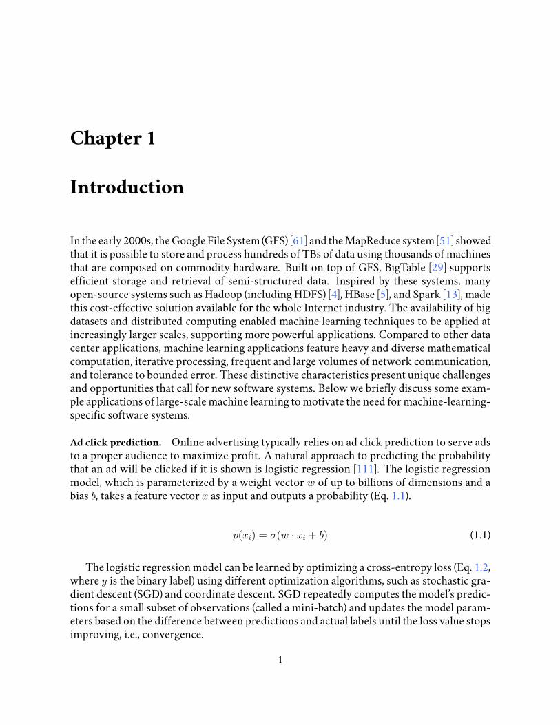
Ad click prediction. Online advertising typically relies on ad click prediction to serve adsto a proper audience to maximize profit. A natural approach to predicting the probabilitythat an ad will be clicked if it is shown is logistic regression [111]. The logistic regressionmodel, which is parameterized by a weight vector w of up to billions of dimensions and abias b, takes a feature vector x as input and outputs a probability (Eq. 1.1).

p(xi) = σ(w · xi + b) (1.1)

The logistic regression model can be learned by optimizing a cross-entropy loss (Eq. 1.2,where y is the binary label) using different optimization algorithms, such as stochastic gra-dient descent (SGD) and coordinate descent. SGD repeatedly computes the model’s predic-tions for a small subset of observations (called a mini-batch) and updates the model param-eters based on the difference between predictions and actual labels until the loss value stopsimproving, i.e., convergence.

1

arg minw,b

L(w, b) = arg minw,b

n∑i=1

yi · log(p(xi)) + (1− yi) · log(1− p(xi)) (1.2)

Recommender systems. Due to the enormous size of their inventory, online shopping, andvideo streaming services, such as Amazon and Netflix, require personalized recommenda-tion to help their customers find relevant merchandise or interesting videos [63]. Recom-mendation systems are popularly built using a matrix factorization model. Given a large(and sparse)m×nmatrix V (e.g., the user-item rating matrix in recommender systems) anda small rank r, the goal of MF is to find an m × r matrix W and an r × n matrix H suchthat V ≈ WH , where the quality of approximation is defined by an application-dependentloss function L. TheW andH matrices can be solved by optimizing a nonzero squared loss(Eq. 1.3)

arg minW,H

LNZSL = arg minW,H

∑i,j:Vij 6=0

(Vij − [WH]ij)2 (1.3)

Topic modeling. Topic modeling discovers the hidden topics of documents and is pop-ularly used in online advertising, search engines, and recommendation systems. LatentDirichlet Allocation (LDA) [26] has become the most popular model for topic modeling.The core of LDA is a topic distribution for each document and a word distribution for eachtopic. The most commonly used learning algorithm for LDA is collapsed Gibbs sampling,which learns the two distributions to maximize the likelihood of a model given the collec-tion of documents. The collapsed Gibbs sampling algorithm sequentially samples a newtopic for each word based on the current distributions and updates the distributions ac-cordingly until the likelihood of the model stops improving.

Image classification. Deep learning has quickly become the most popular class of machinelearning models in the past few years. The first widely successful application of deep learn-ing is image classification [72, 94]. Given an input image, an image classifier outputs a la-bel for that image, e.g., whether the image shows a cat or not. Today, image classifiers arecommonly built using convolutional neural networks, which consist of many computationlayers, and each with its parameters. The parameters in a convolutional neural networkare commonly learned using stochastic gradient descent by minimizing a loss function thatreflects the inaccuracy of the classifier.

Other applications of deep learning. Besides image classification, deep learning has beenapplied to improve the performance of existing machine learning applications and solvenew problems. For example, many ad click prediction systems [70] and recommendationsystems today are enhanced by deep learning [37, 43]. Deep learning achieved real-worldsuccess in many other applications, including, just to name a few, large-scale video ana-lytics [79, 87, 166], machine translation [162], automatic email composition [30] and au-tonomous driving [53].

2

1.1 Characteristics of Machine Learning Training Computation

The above examples show many different models and learning algorithms, but they alsoshare some common characteristics. More importantly, these characteristics are generallyshared by typical machine learning training programs and can be leveraged to improve theexecution efficiency of those programs.

Objective function value

Updates

Asymptote

Convergence

Figure 1.1: Cartoon depicting a typical training process: the model quality, as measured by thetraining objective function, improves over many update steps. The training algorithm convergeswhen the model quality stops improving.

Iterative-convergent search for model parameter values. Most commonly used trainingalgorithms today are iterative-convergent. These algorithms search for model parametervalues to optimize a certain objective function by refining the model parameters in smallsteps until convergence (Fig. 1.1). Due to the iterative-convergent nature of machine learn-ing training, a training algorithm may produce many equally acceptable solutions – a set ofmodel parameter values is considered an acceptable solution as long as the model quality isabove a certain threshold.

Largevolumesof frequent parameter valueupdates. Machine learning training algorithmsare often inherently sequential, where a new model update is computed after the previousupdate is applied. Each update is often computed using a single data sample or a smallmini-batch of data samples, so the training algorithm performs many update steps per passover the training dataset. The training algorithm usually needs many data passes to pro-duce a model that’s good enough. The high frequency of model parameter updates makestraditional batch processing frameworks, such as Spark [174], an inefficient option for dis-tributed ML training due to its immutable data abstraction.

Bounded-error tolerance. Since the training algorithm is an iterative search process, intu-itively, faulty update steps can be compensated for by taking some additional steps as longas the error is properly bounded. One important benefit of bounded error tolerance is thatit offers a trade-off between computation throughput (number of data samples or updatesper second) and computation quality. For example, previous work [75, 127] improve the

3

computation throughput of parallel and distributed training by violating the sequential se-mantics of the training algorithm.

Increasinglyhighmodel complexity. Machine learning is a fast-advancing field. The grow-ing data size encourages researchers and practitioners to design increasingly complex mod-els to improve performance and to support new applications. It is observed that acrossdifferent application domains, more complex models often lead to better prediction accu-racy. For example, over the past several years, winners of the ImageNet image classifica-tion competition have increasingly deep layering, achieving higher accuracy than the pre-vious year’s winner. Besides depth, the increasing model complexity could also be due tolarger layers (e.g., the Mixture of Experts [135]) and new computation-heavy operations,such as Capsule[74]. Due to the increasing model complexity, each update step performsmore and more complex computation, and the training process requires more and morememory to store model parameters and intermediate results. The complex model compu-tation demands more sophisticated optimizations and machine learning frameworks thatemploy fine-grained and informative intermediate representations of computation, such asdataflow graphs, to enable these optimizations.

1.2 Thesis Overview

1.2.1 Thesis Statement

Thesis statement. This thesis describes a set of system techniques that leverage the uniquecharacteristics of machine learning training to improve computation efficiency. Collec-tively, these techniques support the following thesis statement:

Machine learning training may leverage domain-specific opportunities to schedule networkbandwidth, computation, and memory and achieve up to 5× faster training time and enable train-ing up to 7× larger models.

Performance metrics of machine learning training. The performance of most data cen-ter applications, such as batch processing systems, is usually quantified by computationthroughput, which measures the amount of data processed or the number of queries servedper second. Due to the iterative-convergent nature of machine learning training, the timeto find an acceptable model, i.e., time to convergence depends both on the number of up-date steps per second, i.e., computation throughout, and the quality of each update step,i.e., convergence per data sample. Many of our techniques involve trade-offs between com-pute throughput and computation quality; therefore, we evaluate the performance of themachine learning training systems by time to convergence. We evaluate performance bycomputation throughput when such trade-offs are not involved.

Programmable training systems. The described techniques are implemented in Bosen andOrion, which are two distributed training systems that I developed from scratch, and Ten-sorFlow, which is a widely popular deep learning system. These systems support a flexible

4

programming interface for application programmers to implement a wide range of ma-chine learning models and algorithms. Our techniques introduce minimal, or even no, extraburden to application programmers and users. By using automatic parallelization, Orionsubstantially reduces programmer effort for distributed training compared to previous sys-tems.

1.2.2 Contributions

I support the above thesis statement with three major research components.

Scheduling network bandwidth. Distributed machine learning training is often bottle-necked by limited network bandwidth. I design a communication management mechanismto better utilize network bandwidth that improves the convergence speed of distributedtraining. Its key idea is to selectively communicate a subset of messages based on their valuewhen spare network bandwidth is available. This mechanism is implemented in Bosen,which is a Parameter Server system for data-parallel training. Experiments show that itoutperforms the previous state-of-the-art synchronization mechanism by up to 5×. Thisresearch makes the following contributions:

• It introduces Bosen, which is one of the first general-purpose Parameter Server sys-tems for data-parallel training.

• It describes a communication scheduling mechanism to improve inter-machine net-work communication efficiency in data-parallel training to improve convergence time.

• It presents experimental results on a wide range of machine learning models and al-gorithms to demonstrate the effectiveness of communication scheduling.

• As one of the earliest open-source machine learning systems, Bosen provides a testbedfor future research on machine learning systems, such as LightLDA [171] and Posei-don [175].

Scheduling computation. Some model computation sparsely accesses model parameterswhen processing each data sample. Such sparsity may enable parallelization of the trainingalgorithm that preserves its sequential semantics. However, leveraging this opportunityrequires substantial programmer effort to analyze computation dependencies and paral-lelize the training computation manually. I design Orion, which is a new programmingframework to automatically parallelize serial, imperative machine learning programs fordistributed training. When applicable, Orion-parallelized ML programs converge fasterthan manual data-parallelism (even with communication scheduling) due to preserving thesequential semantics. Moreover, Orion falls back to data parallelism when permitted by theprogrammer to parallelize ML programs that are otherwise not sufficiently parallelizable.This research makes the following contributions:

• It introduces a holistic approach for automatically parallelizing serial ML programsfor distributed computation, which includes data abstraction, programming model,

5

and auto-parallelization algorithm. Through this approach, a serial, imperative MLprogram can be parallelized with minimal changes. The auto-parallelization algo-rithm supports semantic relaxations tailored for parallelizing ML programs, whichcan be enabled by programmer hints.

• It describes the system Orion, which is an implementation of the above approach,which parallelizes ML application programs implemented in a scripting language ( Ju-lia [24]). Orion also features a new programming abstraction that unifies dependence-aware parallelization and data parallelism and supports a wide range of ML applica-tions.

• It presents a comprehensive experimental evaluation of Orion that compares Orionwith a number of existing ML systems and demonstrates the effectiveness of Orion’sparallelization.

Scheduling memory. As ML models become more and more complex, ML training de-mands higher and higher memory capacity to store model parameters and intermediatestates. However, GPUs, which are the most widely used deep learning accelerators today,have limited memory, and are highly expensive. I design a memory scheduling mechanismthat leverages the cheap host memory to store model parameters and intermediate results,which are prefetched to GPU memory when needed. In contrast to classic paging tech-niques, we leverage the computation graph to schedule data movement before the data isneeded to avoid stalling GPU computation. Compared to vanilla TensorFlow, our techniqueenables training models with 4.4×more parameters on a single GPU and models with 7.5×more parameters on 4 distributed GPUs. This research makes the following contributions:

• It presents a model-agnostic approach to reduce GPU memory consumption duringtraining by leveraging the cheap host memory. Our approach leverages the generaldataflow graph to reduce the overhead of additional data movements.

• It describes an implementation of our techniques in TensorFlow, which is the mostpopular and most sophisticated deep learning system today. Our implementation doesnot introduce new programming interfaces and supports existing TensorFlow appli-cations without modifications.

• Unlike previous works that are primarily evaluated on convolutional neural networks,we present a comprehensive evaluation across a wide range of deep learning modelsand successfully demonstrate the effectiveness of our approach.

6

Chapter 2

BackgroundConcepts, RelatedWork andTrends

2.1 Distributed Computing Systems

Distributed computing clusters composed of commodity hardware are widely used for data-intensive applications, which are both deployed in private data centers and offered as pub-lic cloud services, e.g., Amazon AWS, Microsoft Azure, and Google GCP. The success ofdistributed computing owes much to sophisticated software systems that make it easy forapplication programmers to leverage the power of the large amount of inexpensive and un-reliable hardware. These software systems include infrastructures that provide resourcesharing among applications and data storage, as well as programming frameworks that tar-get different application domains, such as batch processing, stream processing, and MLtraining. Machine learning systems often interact with other software systems running inthe cluster.

Traditionally, distributed computing clusters consist of hundreds to thousands of CPUservers connected by 1 and 10 Gbps Ethernet. Increasingly more hardware accelerators,such as GPUs and TPUs and new interconnect technologies, such as NVLink, 100 GbpsEthernet, RDMA, and Infiniband, are deployed to meet the growing needs of applicationsin recent years.

Bandwidth bottlenecks. Fig. 2.1 shows the hardware configuration of a node in a dis-tributed cluster deployed at CMU in 2016, which represents the typical characteristics ofcluster servers. Hardware characteristics reveal potential bottlenecks of the software sys-tems running on top of it. First of all, the inter-machine network bandwidth is highly lim-ited. Many older clusters employ Ethernet of 1 Gbit/s, and the network bandwidth on pub-lic clouds is commonly below 10 Gbit/s. Thus it is critical for a distributed system to avoidextensive network communication and make use of this scarce resource carefully. WhileGPU provides high compute power, the bandwidth between GPU and main memory islimited; and the I/O bandwidth between main memory and external storage such as harddrive disks and SSDs is even lower. In earlier systems, CPU cores share one system bus toaccess memory and experience the same bandwidth and latency when accessing different

7

CPU(E5-2698Bv3 Xeon)

Main Memory (DDR4-2133)

68 GB/s

GPU(Titan X Maxwell)

PCIe 3.015.75 GB/s

Memory (GDDR5) Core

336 GB/s

Hard Disk

175 MB/s

SSD

R: 2600 MB/sW: 1700 MB/s

NIC(Ethernet)

40 Gbit/s

Data Center Network

Figure 2.1: The hardware configuration of a node in a distributed cluster deploy at CMU (2016).

memory regions, referred to as Uniform Memory Access (UMA). As the number of CPUcores increases, the per-core bandwith of a UMA system scales poorly due to the limitedscalability of the shared bus. As a solution, Non-Uniform Memory Access (NUMA) systemsemerges, in which each processor has its local memory module (or zone) [9]. A processoraccesses remote memory modules via point-to-point connections between processors, suchas the QPI bus on Intel processors, and experience considerably higher latency and lowerbandwidth (e.g., up to 19.2 GB/s via a QPI bus).

GTX580 Titan Black

Titan X1080 Ti

Titan XpP4000

Titan V

K20cKepler K40 V100-PCIe

T4

Year

$/M

Byte

s

0.005

0.01

0.05

0.1

0.5

1

2000 2005 2010 2015

DRAM Desktop GPU Data Center GPU

Figure 2.2: Comparing DRAM and GPU price. GPU price is presented as dollars per MB of on-board memory. DRAM price was collected by John C. McCallum. 1.

Limited and expensive GPU memory. While originally designed for computer graphics,GPUs are widely used today to accelerate deep learning due to its massively parallel coresand high memory bandwidth. Due to technological limitations, GPU memory cannot pro-

8

vide high bandwidth and high capacity at the same time. GPUs that are most commonlyused for deep learning training today are limited to 12 or 16 GB of memory, and they areexpensive. Fig. 2.2 compares DRAM price with the price of several desktop and server GPUsthat are popularly used for neural network training, in terms of $ per MBytes of on-boardmemory. We observe that GPU price is not affected by the decreasing DRAM price andremains highly expensive. While the recently released Nvidia Tesla V100 GPU has 32 GBof memory2, it’s $1500 more expensive than the 16GB version without additional computepower, leading to a high $0.085 per extra MByte, higher cost than the entire price of themost cost-effective gaming card.

2.2 Preliminaries onMachine Learning Training

Training a model is essentially finding a set of model parameter values that optimize a cer-tain objective function. This is typically done using an iterative convergent learning algo-rithm, which can be described by Alg. 1.

Algorithm 1: Serial Executiont← 0

for epoch = 1,...T dofor i = 1, ..., N do

At+1 ← At ⊕∆ (At,Di)

t← t+ 1

In Alg. 1, At denotes the parameter values at time step t, and Di denotes the i-th mini-batch in the training dataset D = {Di|1 ≤ i ≤ N}. Di may contain one or multiple dataitems. The update function ∆() computes the model updates from a mini-batch of dataitems and the current parameter values, which are applied to generate a new set of param-eter values. ∆ may include some tunable hyperparameters, such as step size in a gradientdescent algorithm, which require manual or automatic tuning for the algorithm to workwell. ⊕ represents the operation to apply parameter updates, which is usually addition. Thealgorithm repeats many times (i.e., epochs) until A stops changing, i.e., converges. In eachepoch, the algorithm takes a full pass over the training dataset.

2.3 Strategies for Distributed Machine Learning Training

2.3.1 Data Parallelism

The most commonly used approach for parallelizing machine learning training is data par-allelism. Data parallelism parallelizes the inner for-loop that iterates over mini-batches Di

by processing many (and even all) mini-batches in parallel with respect to each worker’slocal model state. Note different mini-batches may read and write the same set of model

2Price according to thinkmate.com

9

parameters, and in serial execution, a later mini-batch observes the updates generated bythe previous mini-batches. However, in data parallelism, mini-batches do not observe up-dates from other parallel mini-batches until their updates are propagated to a worker’s localmodel state.

Bulk synchronousparallel. Bulk synchronous parallel (BSP) [147] is a commonly used syn-chronization mechanism for data-parallel training. Under BSP, workers alternate betweencomputation and synchronization. After computing a local computation step, each workerenters a synchronization phase. During the synchronization phase, each worker propagatesupdate messages generated from its local computation to other workers and receives others’updates. Thus the synchronization phase does not end until all workers finish communicat-ing updates. Such a parallelization model is simple but is prone to poor performance sinceall workers proceed at the speed of the slowest worker. The BSP model does not necessarilypreserve a serial algorithm’s sequential semantics unless each worker works on independentcomputation within each iteration.

Due to the iterative nature of machine learning training, in existing literature, the termiteration has been overloaded to refer to a full data pass over the training dataset, i.e., anepoch or a mini-batch, depending on the context. To avoid any confusion, throughout thisthesis, we refer to a full pass over the training dataset as one epoch and use iteration to referto the repeated step in an iterative execution model, such as BSP.

Local buffering. When the model computation is light, computing updates from a singlemini-batch takes little time compared communicating model updates over the bandwidth-limited inter-machine network. Thus communicating once per update step incurs consid-erable communication overhead. Since the model updates are usually additive, the com-munication overhead can be reduced by locally buffering the updates and communicatingupdates once per N update steps, which allows coalescing delta changes to reduce the totalcommunication volume. However, local buffering incurs a higher staleness in parameterstates. Larger staleness causes larger inconsistency compared to serial execution and mayslow down the per-data-sample convergence rate.

Totally asynchronous parallel. In order to overcome the communication overhead andmitigate waiting for stragglers, people also proposed totally asynchronous parallel (TAP) incontrast to BSP. In TAP, a worker propagates parameter updates and fetches new parametervalues (typically from a set of servers referred to as Parameter Server) without waiting forother workers. Additionally, a worker proceeds to the next local computation step usinglocally cached stale parameter states without waiting for the new parameter values. TAPachieves high computation throughput. However, staleness may be arbitrarily large andeven lead to divergence.

Stale synchronous parallel (or bounded staleness). Motivated by the staleness problemsof TAP, stale synchronous parallel (SSP) ensures bounded staleness by blocking a worker’scomputation when its locally cached parameter states are more than T steps stale. This also

10

means the fastest worker cannot be more thanT steps ahead of the slowest worker. Previouswork proves that convergence is guaranteed for certain models when step size is properlytuned [75].

2.3.2 Model Parallelism

Model parallelism broadly refers to parallelization strategies where different workers workon different parts of the model.

Select data samples to process in parallel. Some ML models exhibit a sparse access patternwhere the update computation function ∆ (At,Di) reads and updates a small subset of themodel parameters. By carefully choosing which mini-batches to run in parallel, the parallelworkers work on disjoint subsets of model parameters. As demonstrated by Kim et al. [90],such a parallelization typically preserves the sequential semantics of the learning algorithmand thus achieve a higher per-data-sample convergence rate. However, it usually requiresnon-trivial programmer effort to manually analyze data dependence and implement an ef-ficient distributed program.

Distribute the computation of a single update. For sufficiently complex models, such asdeep neural networks, the update computation ∆ (At,Di) is large enough and thus is worth-while to be parallelized. The computation of ∆() can be distributed among multiple, evenheterogeneous devices. The effectiveness of such parallelization depends on the parallelismof the function ∆ (). DistBelief [52] is an early example of partitioning the model computa-tion across multiple machines. TensorFlow supports user-defined device placement spec-ification at the granularity of individual operations. Mirhoseini et al. [115, 116] and Jia etal. [86] propose different approaches to automate device placement to achieve better train-ing performance. Harlap et al. [71] also leverage pipeline parallelism across mini-batches toimprove the utilization of parallel computing resources.

2.4 RelatedWork

2.4.1 Machine Learning Training Systems

Over the last decade, many systems have been developed for large-scale machine learningtraining. These systems aggressively leverage the application-specific properties of the ma-chine learning models and algorithms to improve system execution efficiency. Machinelearning is a fast-advancing field. New models and algorithms are frequently invented, andthe application domain of machine learning is also fast expanding. Advances in machinelearning introduce new important workloads that pose new challenges and present newopportunities for systems. As a result, large-scale ML systems are fast evolving as well. Inthis chapter, we briefly discuss representative existing machine learning systems, which of-fer insights that can be leveraged by future systems.

11

Distributed Implementations of Machine Learning Applications

Some machine learning models, such as Latent Dirichlet Allocation for topic modeling, havefound diverse and essential use cases in the industry. Such use cases motivate distributedimplementations of such models to enable training on massive datasets. Such systems in-clude Yahoo!LDA [18], Peakcock [155], XGBoost [32], and Caffe [85]. Since they target spe-cific machine learning use cases, they often lack a programming interface and sometimesrely on configuration files to express variations in the model or learning algorithm.

Batch Processing Systems

General-purpose batch processing systems, such as Hadoop [4] and Spark [174], support aprogramming interface for distributed execution. Many attempts were made to implementlarge-scale machine learning training on these systems, including most notably MLLib [8]on Spark. However, these systems are not suitable for machine learning training as they lackan abstraction and efficient implementation for frequently mutated states. This limitationprevents batch processing systems from achieving high training speed and training largemodels.

Graph Processing Systems

The ubiquitous graph datasets draw the attention of data mining and machine learning re-searchers. An early attempt to design a programming interface for machine learning train-ing is thus specialized in graph processing. Notable examples include GraphLab [105], Pow-erGraph [64], GraphChi [96]. These systems feature a vertex programming abstraction,where users implement a vertex program that executes on each vertex of the data graph.The vertex program has a well-defined access pattern, i.e., it may only access neighboringvertices and edges, which enables many opportunities for optimizations, such as partition-ing the data graph to minimize cross-machine communication. While vertex programmingis well suited for many graph mining applications, it is highly restrictive for other machinelearning applications. As machine learning models become more and more complex, andthe model states associated with each vertex and each edge becomes larger, the trainingapplication is more and more bottlenecked by model computation. While the vertex pro-gramming model enables optimizations for disk and network I/O, it is cumbersome forapplication programmers to implement computation optimizations as the vertex programhas only a local view of the computation and states.

General-Purpose Parameter Server Systems

By adopting a distributed shared memory (DSM) abstraction, Parameter Server systems,such as LazyTable [44], IterStore [45], and parameter server [100] provide shared access tomodel parameters among distributed training programs. The low-level and primitive DSMinterface offers great flexibility for machine learning applications but relies on sophisticatedapplication implementations to achieve high computation throughput.

12

Deep Learning Systems

Deep neural networks (DNNs) have become one of the most popular classes of machinelearning models in recent years. A DNN model usually consists of a sequence of cascadedfunctions that transform an input x to some prediction y (Eq. 2.1). Each function (com-monly referred to as a layer) is typically parameterized by a few dense matrices, and thecomputation involves matrix multiplications and additions. The high complexity of matrixoperations and the large number of layers makes it computationally expensive to evaluateDNNs.

y = fn ◦ fn−1... ◦ f1 (x) (2.1)

Many frameworks have been developed for deep learning, including early efforts such asCaffe [85], DistBelief [52], and Project Adam [39]. Caffe and DistBelief represent the neuralnetworks as a sequence of layers and perform fixed training computation over the neuralnetwork definition. This representation makes it difficult for machine learning researchersto define new layers and experiment with new or refined training algorithms. Motivated bythis challenge, modern deep learning frameworks, such as TensorFlow [16] and MXNet [33],represent the neural network computation as a dataflow graph consisting of fine-grainedprimitive operations, which makes it simpler to define new layers and new training algo-rithms. The computation graph provides a global view of the training computation andthus enables many optimization opportunities, such as operator fusion, data layout trans-formation, and dead code elimination. Instead of relying on a computation graph as theintermediate representation, PyTorch [123] offers a more programmer-friendly imperativeprogramming interface but misses the optimization opportunities that a computation graphwould have enabled. As an extension to TensorFlow, TensorFlow Eager [? ] supports imper-ative programming using TensorFlow operations and kernels to lower the burden of Ten-sorFlow users. In order to achieve the high performance of TensorFlow graph execution,TensorFlow Eager introduces a Python decorator function, which traces a Python func-tion to create a computation graph for just-in-time compilation. PyTorch’s JIT compiler(torch.jit.trace) similarly traces the imperative execution to build a computation graphin order to enable automatic differentiation [123]. The aforementioned tracing approachoften fails to correctly capture dynamic features in an imperative Python program, such asdynamic control flow, dynamic data types, and impure functions. JANUS [84] speculativelyexecutes the computation graph that’s constructed by tracing and falls back to imperativeexecution when the actual execution differs from the trace. AutoGraph [117] leverages staticanalysis of the Python code to correctly transform dynamic control flows.

Online Learning Systems

So far, we have focused on batch training systems, where the training data is collected andprepared before training, and a machine learning model is trained from scratch. However,in many applications, the relationship between input data and output labels can change

13

over time, which is referred to as concept drift [59]. When such changes happen too rapidly,it might be too slow or too expensive to re-train the model from scratch to adapt to thechanging environment. Online learning is thus proposed to incrementally update a ma-chine learning model based on new observations while it is served online. One notableexample of online learning is the ad click prediction system deployed at Google [111].

2.4.2 Communication Optimizations for Data-Parallel Training

Overcoming the network communication bottleneck has been a focus of distributed ma-chine learning training systems since the early days and is a focus of this thesis. In thissection, we review the existing literature on communication optimizations for distributedmachine learning training.

Graph Partitioning

In many graph processing applications, the access pattern is characterized by the data graphitself, i.e., processing a vertex reads and updates its neighboring vertices and edges. Parti-tioning the data graph while minimizing cut edges reduces inter-machine communicationvolume [106].

In sparse models such as sparse logistic regression, a subset of model parameters is readand updated when processing each data sample. Placing data samples that share access tomany model parameters on the same machine and placing the accessed model parametersaccordingly reduces inter-machine network communication volume. This access patterncan be characterized as a bipartite graph, and this problem can be solved by partitioningthe graph with minimal edge cut while balancing the size of each partition [101].

Local Buffering

Early graph processing systems [64] and parameter server systems [44, 45, 75] usually ag-gressively buffer updates locally, e.g., synchronize once per epoch (data pass), to reduce thesynchronization overhead. The locally buffered updates can be optionally applied to updatethe worker’s local model cache. The computation-to-communication ratio increases as themachine learning models become more complex, and faster interconnect technologies aredeployed in data centers. Thus local buffering has become less popular for training complexDNNs. However, it remains an important optimization for machine learning under limitednetwork bandwidth, such as in federated learning [112].

Our thesis proposes a mechanism to adaptively tune the network communication fre-quency based on available network bandwidth. Wang et al. [152] verified that the trainingalgorithm, e.g., SGD, tolerates higher staleness in the beginning but becomes more and moresensitive to staleness as the algorithm converges. Therefore, they propose an algorithm toadaptively tune the synchronization frequency based on the learning progress.

14

Data Compression

Data compression has been applied to various types of data to reduce the storage cost andI/O overhead, including images (e.g., JPEG [151]), audio (e.g., MP3 [132]), and video (e.g.,MPEG [38]). Machine learning training enjoys domain-specific opportunities for data com-pression to reduce the communication volume. Xie et al. [164] found that in some machinelearning applications, large dense matrices can be factored into the outer product of twovectors. This lossless compression scheme requires each worker to broadcast its updates toall other workers and thus can be applied to reduce the communication volume on a smallscale.

While Bosen exploits the magnitude of the delta updates to prioritize messages for com-munication when exploiting spare network bandwidth, other parameter server systemsleverage low magnitude to suppress communication when the network bandwidth is highlylimited. Hsieh et al. [78] communicate only updates that are significant enough over WLANsfor efficient geographically distributed training. Aji et al. [20] and Lin et al. [104] proposeto communicate only significant gradients when training DNNs in a data center, droppingor delaying insignificant gradients. Wen et al. [158] show that gradients can often be rep-resented using only 3 bits while achieving reasonable model performance in distributedtraining.

Scheduling Communication Based on Access Pattern

In complex models such as DNNs, the model parameters are not all accessed at the sametime. Parameter synchronization can be scheduled according to the order the parame-ters are accessed in the worker program to avoid blocking communication. Jayarajan etal. [82] demonstrated the effectiveness of this approach on MXNet and showed an up to 66%improvement in computation throughput without sacrificing convergence speed. Peng etal. [124] leverage this idea to build a generic communication scheduler that is applicable toTensorFlow, PyTorch, and MXNet.

2.4.3 Memory Optimizations for Deep Learning

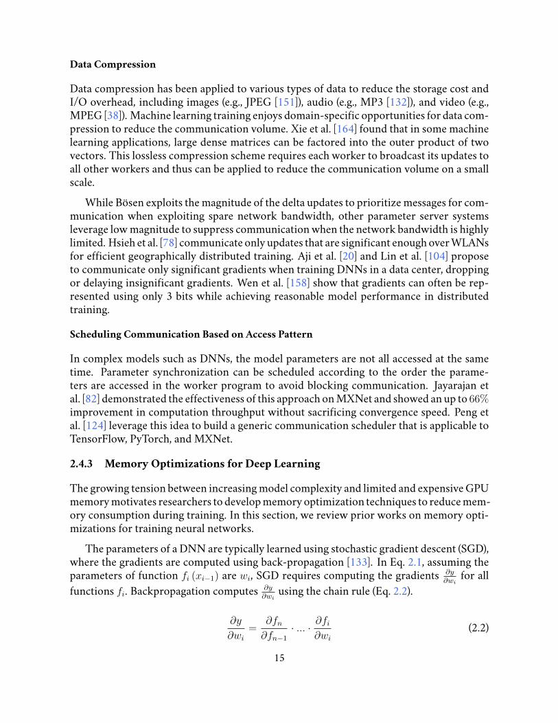
The growing tension between increasing model complexity and limited and expensive GPUmemory motivates researchers to develop memory optimization techniques to reduce mem-ory consumption during training. In this section, we review prior works on memory opti-mizations for training neural networks.

The parameters of a DNN are typically learned using stochastic gradient descent (SGD),where the gradients are computed using back-propagation [133]. In Eq. 2.1, assuming theparameters of function fi (xi−1) are wi, SGD requires computing the gradients ∂y

∂wifor all

functions fi. Backpropagation computes ∂y∂wi

using the chain rule (Eq. 2.2).

∂y

∂wi

=∂fn∂fn−1

· ... · ∂fi∂wi

(2.2)

15

Back-propagation requires the intermediate results fn−1, ..., fi to compute the gradient∂y∂wi

. These intermediate results (often referred to as activation values) can be stored in mem-ory to avoid recomputation. In TensorFlow, this is achieved by reference counting, i.e., thegradient computation operations hold a reference handle to the relevant intermediate re-sults. Storing the intermediate results constitutes the major source of memory consumptionfor many neural networks [128] and becomes the main target for memory optimizations.

Gradient Checkpointing

Chen et al. [35] proposes to checkpoint only a subset of intermediate results in a sequenceof functions, and recompute the rest when necessary to reduce memory consumption. Theidea of trading off recomputation for memory has been investigated in the automatic dif-ferentiation community [67]. Specifically, Chen et al.’s algorithm achieves O(

√N ) memory

consumption at the cost of one additional forward pass for a sequence of N operations bypartitioning the sequence into

√N segments, storing only the outputs of the endpoints, and

recomputing each segment during the backward pass. Gruslys et al. [69] specifically focuson recurrent neural networks and designed a dynamic programming algorithm to maxi-mize computation throughput under memory constraints. Salimans et al. [146] implementChen et al.’s algorithm for TensorFlow applications.

Memory Swapping

During the back-propagation of a mini-batch, not all the parameters and activation valuesare needed at all the time. This observation inspires a series of works to reduce GPU mem-ory consumption by offloading parameters and activation values to cheaper host memoryand loading them only when they are needed. Cui et al. [46] is implemented for Caffe anduses the coarse-grained layer as the unit of swapping operations. Rhu et al. [128] recog-nize that the convolution layers are computationally heavy, and their outputs consume alarge amount of memory, making them a good target for memory offloading. Thus besidesoffloading all layers, Rhu et al. propose another mechanism to offload only convolutionlayers to achieve high computation throughput with higher memory consumption. Wanget al. [153] notice some neural networks are not simply a linear sequence of layers, such asInception [144], and thus linearizes the layers by traversing the neural network in a topolog-ically sorted order. These techniques are applied to coarse-grained layer-wise neural net-work representations and are mostly evaluated on convolutional neural networks. Menget al. [113] describes a memory swapping mechanism for the fine-grained operation-wisegraphs in TensorFlow and TensorFlow’s Grappler memory optimizer implements a sim-ilar memory swapping mechanism [14]. These mechanisms rely on accurate estimationsof operations’ execution time and memory usage and insert memory swapping operationsto the graph when memory swapping does not slow down graph execution based on thesimulation.

16

Mixed Precision and Quantization

Normally the weights, activation values, and gradients in a neural network are representedas 32-bit (single precision) floating-point numbers, i.e., FP32. There have been many previ-ous works on using lower-precision representations for the neural network weights, activa-tions, and gradients to reduce the computation and memory overhead both during trainingand during inference. In this section, we briefly review some most representative works.

Micikevicius et al. [114] store a master copy of the neural network weights in FP32 butuses a 16-bit floating-point (FP16) copy of the weights to compute activations and gradients,which are also stored in FP16. With the help of loss scaling, Micikevicius et al. show thata number of convolutional neural networks can be trained with mixed-precision floating-point numbers without loss of accuracy.

A number of works propose to represent the weights as fixed-point numbers, most com-monly, 8-bit integers (INT8) and perform fixed-point arithmetic for training [42]. Somemore aggressive quantization works represent weights and activations as binary [41] orternary values [98].

Compression

Jain et al. recognizes the output of some important neural network operations such as ReLUlayers followed by a pooling layer and ReLU followed by convolution layers can be losslesslycompressed and achieve a high compression ratio [81]. Jain et al. also performs lossy com-pression on the activations used in the backward pass using low-precision representation.

2.5 Machine Learning Trend: Increasing Model Computation Cost

The focus of large-scale machine learning systems shifts as newer important machine learn-ing models emerge. While traditionally machine learning systems have focused on graphprocessing applications and models such as sparse logistic regression, LDA and matrix fac-torization, which exhibit a sparse parameter access pattern and have low computationalcomplexity for each mini-batch, machine learning systems today are focused on deep neu-ral networks that exhibit a dense parameter access pattern and much higher per-mini-batchcomputational complexity. Advances in the field of machine learning drive the direction ofmachine learning system research.

Amodei et al. [10] at OpenAI calculated the amount of compute (in Petaflop/s-day) neededto train popular deep learning models that are proposed in the past 10 years, which is shownin Fig. 2.3. They argue that the amount of compute used in the largest machine learningtraining runs has been increasing exponentially with a 3.5 month-doubling time. This fastgrowth of the compute needed for training is a direct consequence of the increasing modelcomplexity.

17

Figure 2.3: The computation cost to train stat-of-the-art models in Computer Vision and NaturalLanguage Processing (source: Amodei et al. [10]).

0

5

10

15

20

25

2010 2011 2012 2013 2014 2015 2016

G-FLOPS

Year

AlexNetGoogleNet

VGG-19

Inception-v3

ResNet-152

Figure 2.4: ImageNet competition winners and runner-ups in recent years (source: [3]).

2.5.1 More Complex Models

More complexmodels for better performance. It has been widely observed that across var-ious computer vision and natural language processing applications, more complex modelsachieve higher accuracy. Fig. 2.5 shows some representative deep neural networks that weredeveloped in recent years for image classificiation. Those DNNs lie on a curve starting fromthe lower-left corner and going up to the upper right corner, and the size of the ball, i.e., thenumber of model parameters increases along this direction. This trend indicates that largermodels achieve higher accuracy and incur larger computation overhead. Fig. 2.1 showsthat across different applications, for the same model architecture, increasing model capac-ity improves model accuracy. As a consequence, deep learning models are becoming more

18

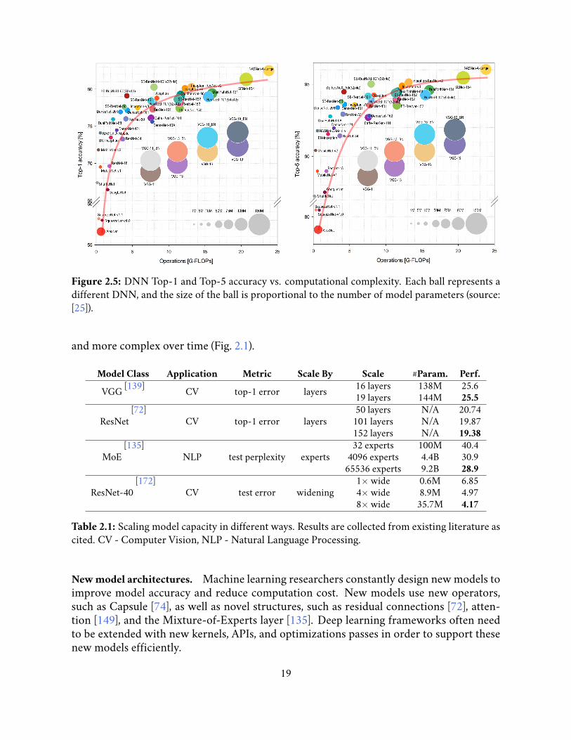
Author et al.: Preparation of Papers for IEEE TRANSACTIONS and JOURNALS

(a) (b)

FIGURE 1: Ball chart reporting the Top-1 and Top-5 accuracy vs. computational complexity. Top-1 and Top-5 accuracy usingonly the center crop versus floating-point operations (FLOPs) required for a single forward pass are reported. The size of eachball corresponds to the model complexity. (a) Top-1; (b) Top-5.

C. MEMORY USAGE

We evaluate the total memory consumption, which includesall the memory that is allocated, i.e. the memory allocated forthe network model and the memory required while process-ing the batch. We measure memory usage for different batchsizes: 1, 2, 4, 8, 16, 32, and 64.

D. COMPUTATIONAL COMPLEXITY

We measure the computational cost of each DNN modelconsidered using the floating-point operations (FLOPs) inthe number of multiply-adds as in [16]. More in detail, themultiply-adds are counted as two FLOPs because, in manyrecent models, convolutions are bias-free and it makes senseto count multiply and add as separate FLOPs.

E. INFERENCE TIME

We report inference time per image for each DNN modelfor both the NVIDIA Titan X Pascal GPU and the NVIDIAJetson TX1. We measure inference time in terms of mil-liseconds and by considering the same batch sizes describedin Section IV-C. For statistical validation the reported timecorresponds to the average over 10 runs.

V. RESULTSA. ACCURACY-RATE VS COMPUTATIONAL

COMPLEXITY VS MODEL COMPLEXITY

The ball charts reported in Figures 1 (a) and (b) show Top-1 and Top-5 accuracy on the ImageNet-1k validation setwith respect to the computational complexity of the con-

sidered architectures for a single forward pass measuredfor both the workstation and the embedded board, The ballsize corresponds to the model complexity. From the plotsit can be seen that the DNN model reaching the highestTop-1 and Top-5 accuracy is the NASNet-A-Large that isalso the one having the highest computational complexity.Among the models having the lowest computational com-plexity instead (i.e. lower than 5 G-FLOPs), SE-ResNeXt-50 (32x4d) is the one reaching the highest Top-1 and Top-5 accuracy showing at the same time a low level of modelcomplexity, with approximately 2.76 M-params. Overall, itseems that there is no relationship between computationalcomplexity and recognition accuracy, for instance SENet-154needs about 3⇥ the number of operations that are neededby SE-ResNeXt-101(32x4d) while having almost the sameaccuracy. Moreover, it seems that there is no relationshipalso between model complexity and recognition accuracy:for instance VGG-13 has a much higher level of modelcomplexity (size of the ball) than ResNet-18 while havingalmost the same accuracy.

B. ACCURACY-RATE VS LEARNING POWER

It is known that DNNs are inefficient in the use of theirfull learning power (measured as the number of parameterswith respect to the degrees of freedom). Although manypapers exist that exploit this feature to produce compressedDNN models with the same accuracy of the original models[24] we want here to measure how efficiently each modeluses its parameters. We follow [4] and measure it as Top-1

VOLUME 4, 2018 3

Figure 2.5: DNN Top-1 and Top-5 accuracy vs. computational complexity. Each ball represents adifferent DNN, and the size of the ball is proportional to the number of model parameters (source:[25]).

and more complex over time (Fig. 2.1).

Model Class Application Metric Scale By Scale #Param. Perf.

VGG [139] CV top-1 error layers 16 layers 138M 25.619 layers 144M 25.5

ResNet[72]

CV top-1 error layers50 layers N/A 20.74

101 layers N/A 19.87152 layers N/A 19.38

MoE[135]

NLP test perplexity experts32 experts 100M 40.4

4096 experts 4.4B 30.965536 experts 9.2B 28.9

ResNet-40[172]

CV test error widening1× wide 0.6M 6.854× wide 8.9M 4.978× wide 35.7M 4.17

Table 2.1: Scaling model capacity in different ways. Results are collected from existing literature ascited. CV - Computer Vision, NLP - Natural Language Processing.

Newmodel architectures. Machine learning researchers constantly design new models toimprove model accuracy and reduce computation cost. New models use new operators,such as Capsule [74], as well as novel structures, such as residual connections [72], atten-tion [149], and the Mixture-of-Experts layer [135]. Deep learning frameworks often needto be extended with new kernels, APIs, and optimizations passes in order to support thesenew models efficiently.

19

2.5.2 Model Selection

The computation cost of machine learning training is amplified by the search for optimaltraining hyperparameters and recently, search for neural network architectures. The searchspace is large due to the inter-dependence between different hyperparameters and networkarchitectures. These search processes involve training multiple versions of the same modelor similar models with different hyperparameters and select the version that achieves thebest accuracy. The high computational cost motivates ML researchers to design new searchalgorithms and system optimizations to reduce the overhead of training many model ver-sions. HiveMind [121] proposes to batch operations and share input data across multiplemodel executions in order to improve the efficiency of hyperparameter search and neuralarchitecture search.

Hyperparameter search. Machine learning training algorithms, such as the widely usedgradient descent algorithm, involve hyperparameters, such as step size. Due to the ambi-guity of the effect of hyperparameter values on model accuracy, grid search with repeatedtrials become the most popular practice. Notable approaches to automate hyperparametersearch and reduce its computation overhead include Spearmint [140], HyperBand [99], andMLtuner [47].

Neural architecture search. Common practices to designing deep learning models ofteninvolve tuning the neural network architecture, for example, changing the number of lay-ers, using different layers, or changing layer sizes. In order to reduce accelerate and improveupon the time-consuming and error-prone model design process by human experts, thereis increasing interest in machine-learning-automated neural architecture search. Generallyspeaking, the machine-learning-automated search trains a controller (often using reinforce-ment learning) that samples task networks (e.g., for image classification) with different ar-chitectures. The task networks are trained to convergence to obtain some accuracy, whichis used as the reward to generate updates to the controller network. Each update to the con-troller involves training multiple task networks, typically in parallel, and each task networkis usually trained using data parallelism. Thus training the controller network demands alarge number of computing resources. For example, Zoph et al. (2017) [179] and Zoph etal. (2018) [180] respectively used 800 and 500 GPUs to train the task networks and took 28days and 4 days to yield the desirable task networks. Recent research, such as ProxyLess-NAS [27], has been devoted to reducing the computation overhead of neural architecturesearch while achieving comparable or even better task model accuracy than previous work.

2.6 Machine Learning Systems Trend: From I/O to Computation

As the machine learning models become more and more complex and training demandsmore and more compute power, machine learning systems emphasize more and more oncomputation. Earlier graph processing systems such as GraphChi [96] and X-Stream [131]focus on reducing the I/O overhead of loading data from external storage as the target ap-plications, such as PageRank, connected components, and triangle counting, traverse the

20

data graph but perform light computation on each vertex. Distributed graph processingsystems, e.g., GraphLab [106] and PowerGraph [64], and Parameter Server systems focuson reducing network communication overhead. As the disk and network I/O overhead re-duces and the computation overhead increases, more and more effort has been devoted tooptimize model computation in deep learning systems, both for training and inference.

In this section, we discuss some promising recent directions in machine learning sys-tems to overcome the computation overhead in DNN training and inference. In particular,these new directions feature machine-learning-guided search to improve upon heuristicsdesigned by domain experts. This machine-learning-guided search measures the compu-tation throughput of a wide range of optimization configurations, which is used to traina model that predicts the computation throughput of a given configuration or outputs theoptimal configuration. It leverages the observation that the same computation graph is re-peatedly applied to all data samples, and thus the computation throughput measured on arandom input is representative of all data samples.

2.6.1 Deep Learning Compilers

Traditionally, deep learning frameworks rely on hand-optimized operation kernels to achievehigh computation efficiency. The diverse set of operations and the complex interactionsbetween them demand optimizations across operation boundaries, such as operator fu-sion and data layout transformation. Therefore, several projects, including TensorFlowXLA [15], propose to optimize DNN models by transforming the computation graph.

However, heuristic-based optimizations are limited by scarce and expensive human timeand thus naturally target standard benchmarks and widely-used models. New models oftenintroduce new operations and expose fresh optimizations opportunities. Moreover, vari-ous custom deep learning accelerators are emerging for deployments in data centers as wellas edge devices. Existing DNNs need to be optimized for new hardware, which exposes dif-ferent architectures and benefits from different optimization heuristics. Hand-optimizedimplementations also involve numerous parameters, such as tile size, which need to be setdifferently for different hardwares. A number of academic and industrial projects try toleverage machine learning to automate optimizations with little to no human interven-tion. Notable examples include TVM [36], PlaidML [11], and Tensor Comprehensions [148].Note that published results are more focused on inference with growing support for train-ing.

Existing dataflow-graph-based representations of DNN models have a number of lim-itations compared to the intermediate representations of general-purpose programminglanguages. For example, dataflow graphs have limited support for dynamic control flowand do not support functions. Deep learning models suffer more and more from theselimitations as the model computation becomes more complex. Recent works, includingMLIR [97] and Relay [130], propose to use more general intermediate representations torepresent DNN computation.

21

2.6.2 Model Parallelism and Device Placement

As DNN models become more and more complex, the model computation is more and morelimited by the computing power and memory capacity of a single computing devices. Dis-tributing the model computation among multiple comnputing device provides a solutionto this bottleneck in many deep learning applications.

TensorFlow [16] relies on application programmers to manually place operations ondevices. GPipe [80] and PipeDream [71] propose to partition the neural network amongdistributed devices in a layer-wise fashion. This coarse-grained partitioning potentiallymisses optimization opportunities and may fail to scale extremely large layers, such as theMixture-of-Experts layer [135]. Mesh-TensorFlow [136] partitions a large operation acrossdistributed computing devices based on a user-provided mesh layout and thus enables train-ing DNNs with operations that have large inputs or outputs. Mirhoseini et al. [115, 116]learn the device placement of individual operations from repeated trial executions of var-ious schedules. Jia et al. [86] simulate the execution to reduce the planning cost down tosub-seconds to tens of minutes depending on the scale (4 to 64 GPUs) and the complexityof the network. Moreover, Jia et al. [86] exploit additional dimensions of parallelization,such as intra-operation parallelism.

22

Chapter 3

Scheduling Inter-Machine Network Communi-cation

As discussed in Sec. 2.3.1, data parallelism is one of the most popular parallelization strate-gies for distributed training, and local buffering is commonly used to balance the param-eter synchronization overhead and convergence rate. An aggressive buffering strategy de-lays parameter synchronization to achieve a high computation throughput but suffers fromslower convergence due to higher staleness in parameter values. While more frequent syn-chronizations may improve convergence rate, the synchronization frequency is ultimatelylimited by the network bandwidth.

In this chapter, I present Bosen, a Parameter Server system that’s designed to better uti-lize the precious network bandwidth for distributed data-parallel training by incorporatingknowledge of network bandwidth and values to be communicated. Bosen adopts Stale Syn-chronous Parallel for parameter synchronization, and in addition, selectively propagatesparameter updates and fresh parameter values in a rate-limited fashion to reduce stalenessin parameter values without congesting the network. The rate-limited communication pri-oritizes parameter updates based on the relative magnitude of the change to allocate thelimited network bandwidth to the most important messages. During machine learningtraining, algorithmic hyperparameters, such as step size, need to be tuned to adapt to thechanging synchronization frequency, in order to take full advantage of the frequent updates.To our knowledge, Bosen is the first distributed implementation of Adaptive Revision [110],a principled step-size tuning algorithm tolerant of delays in distributed systems. AdaptiveRevision achieves theoretical convergence guarantees by adaptively adjusting the step sizeto account for errors caused by delayed updates.

We demonstrate the effectiveness of managed communication on three applications:Matrix Factorization with SGD, Topic Modeling (LDA) with Gibbs sampling, and MulticlassLogistic Regression with SGD on an up to 1024 core compute cluster. Our experiments onMatrix Factorization show orders of magnitude of improvements in the number of itera-tions needed to achieve convergence, compared to the best hand-tuned fixed-schedule stepsize. Even with a delay-tolerant algorithm, Bosen’s managed communication still improves

23

API Description

Get(table, row key, key)Read a single parameter indexed by(row key, key) from table.

GetRow(table, row key)Read a row of parameters indexed byrow key from table.

Inc(table, row key, key, delta)Increment the parameter indexed by(row key, key) from table by delta.

IncRow(row key, deltas)Increment the parameters in row row keyfrom table by deltas.

Clock() Signal the end of a logical clock tick.

Table 3.1: Bosen Client API

the performance of SGD with Adaptive Revision.

3.1 The Bosen Parameter Server Architecture

Bosen is a parameter server with an ML-consistent, bounded-staleness parallel scheme andbandwidth-managed communication mechanisms. It realizes bounded staleness consis-tency, which offers theoretical guarantees for iterative convergent ML programs (unlikeTAP) while enjoying high computation throughput that is better than BSP and close to TAPsystems. Additionally, Bosen transmits model updates and up-to-date model parametersproactively without exceeding a bandwidth limit, while making better use of the bandwidthby scheduling the bandwidth budget based on the contribution of the messages to algorithmprogress — thus improving per-data-sample convergence compared to an agnostic commu-nication strategy.

Bosen PS consists of a client library and parameter server partitions (Figure 3.1);the former provides the Application Programming Interface (API) for reading/updatingmodel parameters, and the latter stores the master copy of the shared model parameters.In terms of usage, Bosen closely follows other key-value stores: once an ML program pro-cess is linked against the client library, any thread in that process may read/update modelparameters concurrently. The user runs a Bosen ML program by invoking as many serverpartitions, and ML application compute processes (which use the client library) as needed,across multiple machines.

Data Abstraction and Bounded Staleness Consistency

Data Abstraction. Bosen represents model parameters and other values that need to beshared among the distributed compute processes as key-value pairs. The application pro-gram create different tables to store values of different types, e.g., floating-point vs. fixed-point, different precision, dense vs. sparse, etc.. In order to exploit locality in ML applica-tions and thus amortize the overhead of concurrent operations, the parameters in a tableare organized into rows – a row is a set of parameters that are usually accessed together. An

24

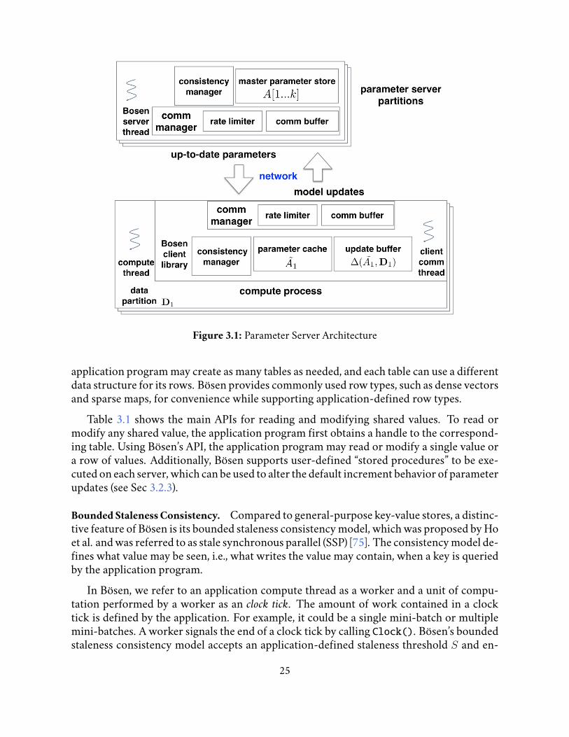
Figure 3.1: Parameter Server Architecture

application program may create as many tables as needed, and each table can use a differentdata structure for its rows. Bosen provides commonly used row types, such as dense vectorsand sparse maps, for convenience while supporting application-defined row types.

Table 3.1 shows the main APIs for reading and modifying shared values. To read ormodify any shared value, the application program first obtains a handle to the correspond-ing table. Using Bosen’s API, the application program may read or modify a single value ora row of values. Additionally, Bosen supports user-defined “stored procedures” to be exe-cuted on each server, which can be used to alter the default increment behavior of parameterupdates (see Sec 3.2.3).

Bounded Staleness Consistency. Compared to general-purpose key-value stores, a distinc-tive feature of Bosen is its bounded staleness consistency model, which was proposed by Hoet al. and was referred to as stale synchronous parallel (SSP) [75]. The consistency model de-fines what value may be seen, i.e., what writes the value may contain, when a key is queriedby the application program.

In Bosen, we refer to an application compute thread as a worker and a unit of compu-tation performed by a worker as an clock tick. The amount of work contained in a clocktick is defined by the application. For example, it could be a single mini-batch or multiplemini-batches. A worker signals the end of a clock tick by calling Clock(). Bosen’s boundedstaleness consistency model accepts an application-defined staleness threshold S and en-

25

clock0 1 2 3 4 5

staleness threshold S = 3

worker 2

worker 1

worker 3

worker 4

current clock tick

guaranteed visible; bounded staleness

worker 2 blocked until worker 1 reaches clock 2

worker 5

visible; updating local cachelikely visible; end of clock communicationnot visible; not yet communicated

Figure 3.2: Exemplar execution under bounded staleness (without communication management).The system consists of 5 workers, with staleness threshold S = 3. Worker 2 is currently running inclock 4, and thus, according to bounded staleness, it is guaranteed to observe all updates generatedin the 4 − 3 − 1 = 0-th clock tick (black). It may also observe local updates (green) as updatescan be optionally applied to local parameter cache. Updates that are generated in completed clocksby other workers (blue) are highly likely visible as they are propagated at the end of each clock.Updates generated in incomplete clocks (white) are not visible as they are not yet communicated.Such updates could be made visible under managed communication depending on the bandwidthbudget.

sures that a worker at the t-th clock tick may observe a parameter a’s value if and only if acontains all updates from the (t − S − 1)-th and earlier clock ticks across all workers. Wesay that a parameter value is too stale with respect to the worker’s logical time if the valueis missing updates from those clock ticks. The worker thread is blocked upon calling Get()or GetRow() until a sufficiently fresh parameter value is available.

Parameter Synchronization. Bosen clients cache parameter values and buffer parameterupdates locally and transmit the buffered updates and fetch fresh parameter values after allapplication compute threads complete a clock tick. All worker threads in a compute processshare a parameter cache, and buffering allows updates generated by different workers overmany clock ticks to be coalesced to reduce communication volume. In order to reducecommunication volume, earlier SSP implementations, such as LazyTable [44, 75], transmitonly parameter updates that are S clocks old and fetch a fresh parameter value only whenthe locally cached value is too stale. In contrast, Bosen transmits all buffered updates andfetches a new value for all parameters needed by this compute process at the end of a clocktick. An exemplary execution of 5 workers under Bounded Staleness is depicted in Fig 3.2.

Machine learning applications typically perform multiple mini-batches within in oneclock tick (i.e., local buffering), especially when each mini-batch is computationally inex-pensive, so parameter synchronization does not become a significant overhead. When thestaleness threshold is set to 0, bounded staleness consistency reduces to the classic BSPmodel. The BSP model guarantees all updates computed in previous clock ticks are visible.

26

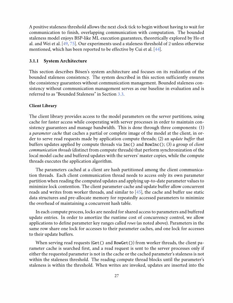
A positive staleness threshold allows the next clock tick to begin without having to wait forcommunication to finish, overlapping communication with computation. The boundedstaleness model enjoys BSP-like ML execution guarantees, theoretically explored by Ho etal. and Wei et al. [49, 75]. Our experiments used a staleness threshold of 2 unless otherwisementioned, which has been reported to be effective by Cui et al. [44].

3.1.1 System Architecture

This section describes Bosen’s system architecture and focuses on its realization of thebounded staleness consistency. The system described in this section sufficiently ensuresthe consistency guarantees without communication management. Bounded staleness con-sistency without communication management serves as our baseline in evaluation and isreferred to as “Bounded Staleness” in Section 3.3.

Client Library

The client library provides access to the model parameters on the server partitions, usingcache for faster access while cooperating with server processes in order to maintain con-sistency guarantees and manage bandwidth. This is done through three components: (1)a parameter cache that caches a partial or complete image of the model at the client, in or-der to serve read requests made by application compute threads; (2) an update buffer thatbuffers updates applied by compute threads via Inc() and RowInc(); (3) a group of clientcommunication threads (distinct from compute threads) that perform synchronization of thelocal model cache and buffered updates with the servers’ master copies, while the computethreads executes the application algorithm.

The parameters cached at a client are hash partitioned among the client communica-tion threads. Each client communication thread needs to access only its own parameterpartition when reading the computed updates and applying up-to-date parameter values tominimize lock contention. The client parameter cache and update buffer allow concurrentreads and writes from worker threads, and similar to [45], the cache and buffer use staticdata structures and pre-allocate memory for repeatedly accessed parameters to minimizethe overhead of maintaining a concurrent hash table.

In each compute process, locks are needed for shared access to parameters and bufferedupdate entries. In order to amortize the runtime cost of concurrency control, we allowapplications to define parameter key ranges called rows (as noted above). Parameters in thesame row share one lock for accesses to their parameter caches, and one lock for accessesto their update buffers.

When serving read requests (Get() and RowGet()) from worker threads, the client pa-rameter cache is searched first, and a read request is sent to the server processes only ifeither the requested parameter is not in the cache or the cached parameter’s staleness is notwithin the staleness threshold. The reading compute thread blocks until the parameter’sstaleness is within the threshold. When writes are invoked, updates are inserted into the

27

update buffer, and, optionally, the client’s own parameter cache is also updated.Once all compute threads in a client process have called Clock() to signal the end of

a unit of work (e.g., a clock tick), the client communication threads release buffered modelupdates to servers. Note that buffered updates may be released sooner under managed com-munication if the system detects spare network bandwidth to use.

Server Partitions

The master copy of the model’s parameters is hash partitioned, and each partition is as-signed to one server thread. The server threads may be distributed across multiple serverprocesses and physical machines. As model updates are received from client processes, theaddressed server thread updates the master copy of its model partition. When a client readrequest is received, the corresponding server thread registers a callback for that request;once a server thread has applied all updates from all clients for a given unit of work, itwalks through its callbacks and sends up-to-date model parameter values.

Ensuring Bounded Staleness

Bounded staleness is ensured by coordination of clients and server partitions using clockmessages. On an individual client, as soon as all updates generated before and in the t-thclock tick are sent to server partitions and no more updates before or in that clock tick canbe generated (because all compute threads have advanced beyond that clock), the client’scommunication threads send a client clock message to each server partition, indicating “allupdates generated before and in clock t by this client have been made visible to this serverpartition” (assuming reliable, ordered message delivery).

After a server partition sends out all dirty parameters modified in clock t, it sends aserver clock message to each client communication thread, indicating ‘all updates generatedbefore and in clock t in the parameter partition have been made visible to this client”. Uponreceiving such a clock message, the client communication thread updates the age of thecorresponding parameters and permits the relevant blocked compute threads to proceedon reads, if any.

Fault Tolerance

Bosen provides fault tolerance by checkpointing the server model partitions; in the eventof failure, the entire system is restarted from the last checkpoint. A valid checkpoint con-tains the model state strictly right after clock t— the model state includes all model updatesgenerated before and during clock t, and excludes all updates after the t-th Clock() call byany worker thread. With bounded staleness, clients may asynchronously enter new clocksand begin sending updates; thus, whenever a checkpointing clock event is reached, eachserver model partition will copy-on-write protect the checkpoint’s parameter values un-til that checkpoint has been successfully copied externally. Since taking a checkpoint canbe slow, a checkpoint will not be made every clock or even every few clocks. A good es-

28

timate of the amount of time between taking checkpoints is√

2TsTf/N [168], where Ts isthe meantime to save a checkpoint, there are N machines involved and Tf is the meantimeto failure (MTTF) of a machine, typically estimated as the inverse of the average fraction ofmachines that fail each year.

As Bosen targets offline batch training, restarting the system (disrupting its availability)is not critical. With tens or hundreds of machines, such training tasks typically complete inhours or tens of hours. Considering the MTTF of modern hardware, it is not necessary tocreate many checkpoints, and the probability of restarting is low. In contrast, a replication-based fault tolerance mechanism inevitably costs 2× or even more memory on storing thereplicas and additional network bandwidth for synchronizing them.

3.2 Managed Communication

Bosen’s client library and server partitions feature a communication manager whose pur-pose is to improve ML progress per epoch (i.e., data pass) through careful use of networkbandwidth in communicating model updates/parameters. Communication management iscomplementary to consistency management; the latter prevents worst-case behavior frombreaking ML consistency (correctness), while the former improves convergence time (speed).

The communication manager has two objectives: (1) communicate as many updates persecond as possible (full utilization of the bandwidth budget) without overusing the network(which could delay update delivery and increase message processing computation over-head); and (2) prioritize more important model updates to improve ML progress per epoch.The first objective is achieved via bandwidth-driven communication with rate limiting,while the second is achieved by choosing a proper prioritization strategy.

3.2.1 Bandwidth-Driven Communication

Similar to the leaky bucket model, the Bosen communication manager models the networkas a bucket that leaks bytes at a certain rate and the leaky rate corresponds to the node’sbandwidth consumption. Thus the leaky rate is set to the given bandwidth budget to con-strain the average bandwidth consumption. In order to fully utilize the given bandwidthbudget, the communication manager permits communication of updates or updated pa-rameters whenever the bucket becomes empty (and thus communication may happen be-fore the completion of a clock tick). The communication manager keeps track of the numberof bytes sent last time to monitor the state of the bucket. In our prototype implementation,the communication threads periodically query the communication manager for opportu-nities to communicate. The size of each send is limited by the size of the bucket (referredto as “queue size”) to control its burstiness.

Copingwithnetwork fluctuations. In real cloud data centers with multiple users, the avail-able network bandwidth may fluctuate and fail to live up to the bandwidth budgetB. Hence,the Bosen communication manager regularly checks to see if the network is overused bymonitoring how many messages were sent without acknowledgment in a recent time win-

29

dow (i.e., message non-delivery). If too many messages fail to be acknowledged, the com-munication manager assumes that the network is overused, and waits until the windowbecomes clear before permitting new messages to be sent.

Update quantization. As we discussed in Sec. 2.4.3, there has been a growing body of workin recent years that uses reduced precision and quantization to represent floating-pointnumbers to reduce the overhead of communicatig model updates. Bosen applications havethe option to use IEEE half-precision 16-bit floating-point numbers for communication,reducing bandwidth consumption in half compared to 32-bit floats. The lost informationoften has a negligible impact on progress per epoch.

3.2.2 Update Prioritization

Bosen spends available bandwidth on communicating information that contributes the mostto convergence. For example, gradient-based algorithms (including Logistic Regression)are iterative-convergent procedures in which the fastest-changing parameters are often thelargest contributors to solution quality — in this case, we prioritize communication of fast-changing parameters, with the largest-magnitude changes going out first. When there is anopportunity for communication due to spare bandwidth, the server or client communica-tion threads pick a subset of parameter values or updates to send. The prioritization strategydetermines which subset is picked at each communication event. By picking the right subsetto send, the prioritization strategy alters the communication frequency of different param-eters, effectively allocating more network bandwidth to more important updates. It shouldbe noted that the end-of-clock communication needs to send all up-to-date parameters orupdates older than a certain clock number to ensure the consistency guarantees.

Bosen’s bandwidth manager supports multiple prioritization strategies. The simplestpossible strategies are Randomized, where communications threads send out randomly-chosen rows and Round-Robin, where communication threads repeatedly walk throughthe rows following a fixed order, and sends out all non-zero updates or updated param-eters encountered. These strategies are baselines; better strategies prioritize according tosignificance to convergence progress. We study the following two better strategies.

Absolute Magnitude prioritization. Updates/parameters are sorted by their accumulatedchange in the buffer, |δ|.

Relative Magnitude prioritization. Same as absolute magnitude, but the sorting criteriais |δ/a|, i.e., the accumulated change normalized by the current parameter value, a. Forsome ML problems, relative change |δ/a|may be a better indicator of progress than absolutechange |δ|. In cases where a = 0 or is not in the client parameter cache, we fall back toabsolute magnitude prioritization.

30

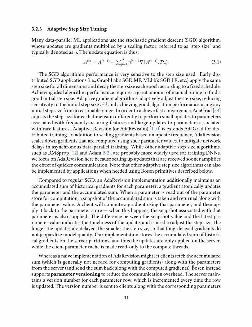
3.2.3 Adaptive Step Size Tuning

Many data-parallel ML applications use the stochastic gradient descent (SGD) algorithm,whose updates are gradients multiplied by a scaling factor, referred to as “step size” andtypically denoted as η. The update equation is thus:

A(t) = A(t−1) +∑P

p=1 η(t−1)p ∇(A(t−1),Dp). (3.1)

The SGD algorithm’s performance is very sensitive to the step size used. Early dis-tributed SGD applications (i.e., GraphLab’s SGD MF, MLlib’s SGD LR, etc.) apply the samestep size for all dimensions and decay the step size each epoch according to a fixed schedule.Achieving ideal algorithm performance requires a great amount of manual tuning to find agood initial step size. Adaptive gradient algorithms adaptively adjust the step size, reducingsensitivity to the initial step size η(1) and achieving good algorithm performance using anyinitial step size from a reasonable range. In order to achieve fast convergence, AdaGrad [54]adjusts the step size for each dimension differently to perform small updates to parametersassociated with frequently occuring features and large updates to parameters associatedwith rare features. Adaptive Revision (or AdaRevision) [110] is extends AdaGrad for dis-tributed training. In addition to scaling gradients based on update frequency, AdaRevisionscales down gradients that are computed using stale parameter values, to mitigate networkdelays in asynchronous data-parallel training. While other adaptive step size algorithms,such as RMSprop [12] and Adam [92], are probably more widely used for training DNNs,we focus on AdaRevision here because scaling up updates that are received sooner amplifiesthe effect of quicker communication. Note that other adaptive step size algorithms can alsobe implemented by applications when needed using Bosen primitives described below.

Compared to regular SGD, an AdaRevision implementation additionally maintains anaccumulated sum of historical gradients for each parameter; a gradient atomically updatesthe parameter and the accumulated sum. When a parameter is read out of the parameterstore for computation, a snapshot of the accumulated sum is taken and returned along withthe parameter value. A client will compute a gradient using that parameter, and then ap-ply it back to the parameter store — when this happens, the snapshot associated with thatparameter is also supplied. The difference between the snapshot value and the latest pa-rameter value indicates the timeliness of the update, and is used to adjust the step size: thelonger the updates are delayed, the smaller the step size, so that long-delayed gradients donot jeopardize model quality. Our implementation stores the accumulated sum of histori-cal gradients on the server partitions, and thus the updates are only applied on the server,while the client parameter cache is made read-only to the compute threads.

Whereas a naive implementation of AdaRevision might let clients fetch the accumulatedsum (which is generally not needed for computing gradients) along with the parametersfrom the server (and send the sum back along with the computed gradients), Bosen insteadsupportsparameter versioning to reduce the communication overhead. The server main-tains a version number for each parameter row, which is incremented every time the rowis updated. The version number is sent to clients along with the corresponding parameters

31

1e+

08

1e+

09

1e+

10

0 10 20 30 40 50 60

train

ing loss

iterations

BStale, AdaRev, Eta=0.08BStale, AdaRev, Eta=0.1BStale, AdaRev, Eta=0.4

BStale, MultiDecay, Eta=6e-5BStale, MultiDecay, Eta=1.2e-5

GraphLab, Sync, Eta=1e-5

Figure 3.3: Compare Bosen’s SGD MF w/ and w/o adaptive revision with GraphLab SGD MF. Etadenotes the initial step size. Multiplicative decay (MultiDecay) used its optimal initial step size.

and stored in the client’s parameter cache. The update computed (by a worker) for parame-ter i is tagged with the version number of parameter i in the parameter cache. The updatestagged with the same version number are aggregated via addition as usual, but updates withdifferent version numbers are stored separately. The use of version number to indicate thetimeliness of writes is similar to optimistic concurrency control.

The AdaRevision algorithm is implemented as auser-defined storedprocedure (UDF)on the server. The user-defined stored procedure contains a set of user-implemented func-tions that are invoked at various events to control the server’s behavior. Most notably, theUDF takes snapshots of the accumulated sum of the historical gradients and increments theversion number upon sending parameters to clients and computes the step size when ap-plying gradients. In order to bound the overall memory usage, the UDF imposes an upperlimit on the number of snapshots that can be kept. Bandwidth-triggered communicationis canceled upon exceeding this limit. The snapshots are freed when no client cache stillcontains this version of the parameter

We demonstrate the importance of step size tuning and effectiveness of adaptive revisionusing the SGD MF application on the Netflix dataset, with rank = 50, using one node in thePRObE Susitna cluster (see Sec 3.3). As shown in Fig. 3.3, we compared adaptive revision(AdaRev) with Multiplicative Decay (MultiDecay) using various initial step sizes. We alsoran GraphLab’s SGD MF using its synchronous engine (the asynchronous engine convergesslower per epoch) with a range of initial step sizes from 1e−4 to 1e−6 and showed its bestconvergence result.

Firstly, we observed that multiplicative decay is sensitive to the initial step size. Chang-ing the initial step size from 6e−5 to 1.2e−5 reduces the number of epochs needed to reach

32

Dataset Workload Description Data SizeNetflix 100M ratings 480K users, 18K movies, rank=400 1.3GB

NYTimes 99.5M tokens 300K documents, 100K words 1K topics 0.5GBClueWeb10% 10B tokens 50M webpages, 160K words, 1K topics 80GBImageNet5% 65K samples 1000 classes, 21K of feature dimensions 5.1GB

Table 3.2: Datasets used in evaluation. Data size refers to the input data size. Workload refers to thetotal number of data samples in the input data set.

Application Dataset # Rows Row SizeSGD MF Netflix 480K 1.6KB

LDA NYTimes 100K dynamicLDA ClueWeb10% 160K dynamicMLR ImageNet5% 1K 84KB

Table 3.3: Descriptions of ML models and evaluation datasets. The overall model size is thus # Rowsmultiplied by row size.

Application & Dataset # Machines Bandwidth Budgets Queue SizeSGD MF, Netflix 8 (N) 200Mbps, 800Mbps 100, 100

LDA, NYTimes 16 (N) 320Mbps, 640Mbps, 1280Mbps 5000, 500

LDA, ClueWeb10% 64 (N) 800Mbps 5000, 500

MLR, ImageNet5% 4 (S) 100Mbps, 200Mbps, 1600Mbps 1000, 500

Table 3.4: Bosen system and application configurations. N - cluster Nome, S - cluster Susitna. Thequeue size (in number of rows) upper bounds the send size to control burstiness; the first numberdenotes that for client and the second for server. LDA experiments used hyper-parameters α = β =

0.1. SGD MF and MLR uses an initial learning rate of 0.08 and 1 respectively.

a training loss of 1e8 by more than 3×. However, convergence with adaptive revision ismuch more robust, and the difference between the initial step size of 0.08 and 0.4 is neg-ligible. Secondly, we observed that SGD MF under adaptive revision converges 2× fasterthan using multiplicative decay with the optimal initial step size that our manual parametertuning could find. Even though GraphLab also applies multiplicative decay to its step size,it does not converge well.

The adaptive revision algorithm becomes more effective when scaling the SGD appli-cation as it adapts the step size to tolerate the communication delay. An experiment (notshown) using 8 Susitna nodes shows that adaptive revision reduces the number of epochsto convergence by 10×.

3.3 Evaluation

We evaluated Bosen using three real machine learning applications, matrix factorization(MF) solved by SGD, latent Dirichlet allocation (LDA) solved by collapsed Gibbs sampling,

33

Application & Dataset Result FiguresSGD MF, Netflix 3.4a, 3.6a, 3.7aLDA, NYTimes 3.4b, 3.6b, 3.10

MLR, ImageNet5% 3.7b

Table 3.5: Summary of experiment result figures.

and multiclass logistic regression (MLR) also solved by SGD.Cluster setup: Most of our experiments were conducted on PRObE Nome [62], consistingof 200 computers running Ubuntu 14.04. Our experiments used different numbers of com-puters, varying from 8 to 64. Each machine contains 4 × quad-core AMD Opteron 8354CPUs (16 physical cores per machine) and 32GB of RAM. The machines were distributedover multiple racks and connected via a 1 Gb Ethernet and 20 Gb Infiniband. A few exper-iments were conducted on PRObE Susitna [62]. Each machine contains 4 × 16-core AMDOpteron 6272 CPUs (64 physical cores per machine) and 128GB of RAM. The machinesare distributed over two racks and connected to two networks: 1 GbE and 40 GbE. In bothclusters, every machine is used to host Bosen server, client library, and worker threads (i.e.,servers and clients are collocated and evenly distributed).ML algorithm setup: In all ML applications, we partition the data samples evenly acrossthe workers. Unless otherwise noted, we adopted the typical BSP configuration and con-figured 1 logical clock tick to be 1 pass through the worker’s local data partition1. The MLmodels and datasets are described in Table 3.3, and the system and application configura-tions are described in Table 3.4.Performancemetrics: Our evaluation measures performance as the absolute convergencerate on the training objective value; that is, our goal is to reach convergence to an estimateof the model parameters that best represent the training data (as measured by the trainingobjective value) in the shortest time.

Bosen is executed under different modes in this section:Single Node: The ML application is run on one shared-memory machine linked againstone Bosen client library instance with only consistency management. The parameter cacheis updated upon write operations. Thus updates become immediately visible to computethreads. It represents a gold standard when applicable. It is denoted as “SN”.Linear Scalability: It represents an ideal scenario where the single-node application isscaled out, and linear scalability is achieved. It is denoted as “LS”.Bounded Staleness: Bosen is executed with only consistency management enabled, andcommunication management is disabled. It is denoted as “BS”.Bounded Staleness + Managed Communication: Bosen is executed with both consis-

1In one clock we compute parameter updates using each of the N data samples in the dataset exactly once, regardlessof the number of parallel workers. With more workers, each worker will touch fewer data samples per data pass.

34

tency and communication management enabled. It is denoted as “MC-X-P”, where X de-notes the per-node bandwidth budget (in Mbps), and P denotes the prioritization strategy:“R” for Randomized, “RR” for Round-Robin, and “RM” for Relative-Magnitude.Bounded Staleness + Fine-Grained Clock Tick Size: Bosen is executed with only con-sistency management enabled, communication management is disabled. In order to com-municate updates and model parameters more frequently, a full pass over data is dividedinto multiple clock tick. It is denoted as “BS-X”, where X is the number of clock ticks thatconstitutes a data pass.

Unless otherwise mentioned, we used a staleness threshold of 2 and we found that al-though bounded staleness converges faster than BSP, changing the staleness threshold doesnot affect average-case performance as the actual staleness is usually 1 due to the eagerend-of-clock communication (Section 3.1). The network waiting time is small enough thata staleness threshold of 2 achieves no blocking. The bounded staleness consistency modelallows computation to proceed during synchronization. As long as the workload is balancedand synchronization completes within one clock tick of computation (which is typically thecase), the network waiting time can be completely hidden.

3.3.1 CommunicationManagement

In this section, we show that the algorithm performance improves with more immediatecommunication of updates and model parameters. Moreover, proper bandwidth allocationbased on the importance of the messages may achieve better algorithm performance withless bandwidth consumption. To this end, we compared managed communication withnon-managed communication (i.e., only the consistency manager is enabled). The com-munication management mechanism was tested with different per-node bandwidth bud-gets (see Table 3.4) and different prioritization strategies (Section 3.2.2). Each node runsthe same number of client and server communication threads and the bandwidth budget isevenly divided among them.Effect of increasing bandwidth budget. Under Bosen’s communication management, in-creasing bandwidth budget permits more immediate communication of model updates andparameters and thus improves algorithm performance (higher convergence per epoch, i.e.,data pass) given a fixed prioritization policy. We demonstrate this effect via the MF and LDAexperiments (Fig. 3.4). First of all, we observed that enabling communication managementsignificantly reduces the number of epochs needed to reach convergence (objective value of2e7 for MF and −1.022e9 for LDA). In MF, communication management with bandwidthbudget of 200Mbps reduces the number of epochs needed to reach 2e7 from 64 (BS) to 24(MC-200-R). In LDA, a bandwidth budget of 320Mbps reduces the number of epochs toconvergence from 740 (BS) to 195 (MC-320-R). Secondly, increasing the bandwidth budgetfurther reduces the number of epochs needed. For example, in LDA, increasing the band-width budget from 320Mbps (MC-320-R) to 640Mbps (MC-640-R) reduces the numberepochs needed from 195 to 120.

35

1e+

07

1e+

08

1e+

09

0 10 20 30 40 50 60

train

ing

loss

iterations

BSMC-200-R

MC-200-RMMC-800-R

MC-800-RMMC-800-RR

(a) SGD Matrix Factorization

0

100

200

300

400

500

600

700

800

SN BS

MC-320-R

MC-320-RM

MC-640-R

MC-640-RM

MC-1280-R

itera

tions

(b) Topic Modeling (LDA), number of epochs to convergence

Figure 3.4: Algorithm performance under managed communication

Effect of prioritization. As shown Fig. 3.4b, in the case of LDA, prioritization by Relative-Magnitude (RM) consistently improves upon Randomization (R) when using the same amountof bandwidth. For example, with 320Mbps of per-node bandwidth budget MC-320-RM re-duces the number of epochs needed to reach −1.022e9 from 195 (MC-320-R) to 145.

Relative-Magnitude prioritization improves upon Randomized prioritization as it dif-ferentiates updates and model parameters based on their significance to algorithm perfor-mance. It allocates network bandwidth accordingly and communicates different updatesand model parameters at different frequencies. Fig. 3.5 shows the CDFs of communicationfrequency of LDA’s model parameters, under different policies. For the NYTimes dataset,we observed that Relative-Magnitude and Absolute-Magnitude prioritization achieve sim-ilar effect, where a small subset of keys are communicated much more frequently. Randomand Round-Robin achieve similar effect where all keys are communicated at roughly the

36

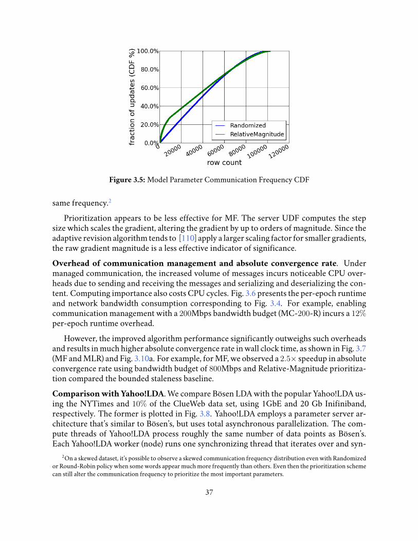
Figure 3.5: Model Parameter Communication Frequency CDF

same frequency.2

Prioritization appears to be less effective for MF. The server UDF computes the stepsize which scales the gradient, altering the gradient by up to orders of magnitude. Since theadaptive revision algorithm tends to [110] apply a larger scaling factor for smaller gradients,the raw gradient magnitude is a less effective indicator of significance.Overhead of communication management and absolute convergence rate. Undermanaged communication, the increased volume of messages incurs noticeable CPU over-heads due to sending and receiving the messages and serializing and deserializing the con-tent. Computing importance also costs CPU cycles. Fig. 3.6 presents the per-epoch runtimeand network bandwidth consumption corresponding to Fig. 3.4. For example, enablingcommunication management with a 200Mbps bandwidth budget (MC-200-R) incurs a 12%per-epoch runtime overhead.

However, the improved algorithm performance significantly outweighs such overheadsand results in much higher absolute convergence rate in wall clock time, as shown in Fig. 3.7(MF and MLR) and Fig. 3.10a. For example, for MF, we observed a 2.5× speedup in absoluteconvergence rate using bandwidth budget of 800Mbps and Relative-Magnitude prioritiza-tion compared the bounded staleness baseline.Comparisonwith Yahoo!LDA. We compare Bosen LDA with the popular Yahoo!LDA us-ing the NYTimes and 10% of the ClueWeb data set, using 1GbE and 20 Gb Inifiniband,respectively. The former is plotted in Fig. 3.8. Yahoo!LDA employs a parameter server ar-chitecture that’s similar to Bosen’s, but uses total asynchronous parallelization. The com-pute threads of Yahoo!LDA process roughly the same number of data points as Bosen’s.Each Yahoo!LDA worker (node) runs one synchronizing thread that iterates over and syn-

2On a skewed dataset, it’s possible to observe a skewed communication frequency distribution even with Randomizedor Round-Robin policy when some words appear much more frequently than others. Even then the prioritization schemecan still alter the communication frequency to prioritize the most important parameters.

37

0

5

10

15

20

25

30

35

40

BS

MC-200-R

MC-200-RM

MC-800-R

MC-800-RM BS

MC-200-R

MC-200-RM

MC-800-R

MC-800-RM

0

100

200

300

400

500

600

700

800

time per data

pass (seconds)

average bandwidth

(Mbps)

computewait

bw

bandwidthtime

(a) SGD Matrix Factorization

0

1

2

3

4

5

6

7

BS

MC-320-R

MC-320-RM

MC-640-R

MC-640-RM

MC-1280R BS

MC-320-R

MC-320-RM

MC-640-R

MC-640-RM

MC-1280R

0

100

200

300

400

500

600

time per data

pass (seconds)

average bandwidth

(Mbps)

computewait

bw

bandwidthtime

(b) Topic Modeling (LDA)

Figure 3.6: Overhead of communication management: time per data pass and average bandwidthconsumption. Note that while managed communication consumes high network bandwidth andtakes longer to perform a mini-batch, it significally reduces the number of epoches needed to reachthe target objective function value (see Fig. 3.4) and thus improves the wall clock time to convergence(see Fig. 3.7)

chronizes all cached parameter in a predefined order. We observed that Bosen significantlyoutperformed Yahoo!LDA on the NYTimes dataset, but converged at similar rate on theClueWeb10% data set.

In summary, by making full use of the 800Mbps and 640Mbps bandwidth budget, com-

38

1e+

07

1e+

08

1e+

09

0 500 1000 1500 2000 2500

train

ing

loss

seconds

BSMC-200-R

MC-200-RMMC-800-R

MC-800-RMMC-800-RR

(a) SGD Matrix Factorization

0 2

4 6

8 1

0 1

2 1

4 1

6

0 1000 2000 3000 4000 5000 6000 7000 8000

train

ing

loss

seconds

LSBS

MC-100-RMC-200-R

MC-200-RMMC-16000-R

(b) Multi-class Logistic Regression

Figure 3.7: Absolute convergence rate under managed communication

munication management with Randomized prioritization improved the time to conver-gence of the MF and LDA application by 2.5× and 2.8× in wall clock time and 5.3× and6.1× in number of epochs, compared to a bounded staleness execution. Relative-Magnitudeprioritization further improves the convergence time of LDA by 25%. Communicationmanagement with bandwidth budget of 200Mbps and Relative-Magnitude prioritizationimproved the convergence time of MLR by 2.5×.

3.3.2 Comparison with Clock Tick Size Tuning

Another way of reducing parallel error on a BSP or bounded staleness system is to dividea full data pass into multiple clock ticks to achieve more frequent synchronization, whileproperly adjusting the staleness threshold to ensure the same staleness bound. This ap-proach is similar to mini-batch size tuning in ML literature. In this section, we compare

39

-1.5

5e+09

-1.5

e+09

-1.4

5e+09

-1.4

e+09

-1.3

5e+09

-1.3

e+09

-1.2

5e+09

-1.2

e+09

-1.1

5e+09

-1.1

e+09

-1.0

5e+09-1

e+09

0 500 1000 1500 2000

log

-lik

lihood

seconds

Bosen, BSBosen, MC-640-RM

Yahoo!LDA

Figure 3.8: Compare Bosen LDA with Yahoo!LDA on NYTimes Data

-1.1

4e+09-1

.12e

+09-1

.1e+

09-1.0

8e+09-1

.06e

+09-1

.04e

+09-1

.02e

+09

-1e+

09

0 50 100 150 200 250 300

log

-lik

lihood

seconds

Bounded Staleness (S)Bounded Staleness, C=2 (S(2))Bounded Staleness, C=4 (S(4))Bounded Staleness, C=8 (S(8))

Bosen, 320Mbps, R (B1)Bosen, 640Mbps, RM (B2)

Figure 3.9: Comparing Bosen with simply tuning clock tick size: convergence per epoch

Bosen’s communication management with application-level clock tick size tuning via theLDA application and the result is plotted in Fig 3.10. For each number of clock ticks perdata pass, we adjust the staleness threshold so all runs share the same staleness bound of 2data passes.

Firstly, from Fig. 3.10a we observe that as the clock tick size halves, the average band-width usage over the first 280 epochs doubles but the average time per epoch doesn’t changesignificantly. From Fig. 3.9, we observe that the increased communication improves the al-gorithm performance. Although simply tuning clock tick size also improves algorithm be-havior, it doesn’t enjoy the benefit of prioritization. For example, MC-640-RM used only

40

0

500

1000

1500

2000

2500

3000

BSBS-2 BS-4 BS-8

MC-320-R

MC-320-RM

MC-640-R

MC-640-RM

seco

nd

s

(a) time to convergence

0 0.5

1 1.5

2 2.5

3 3.5

4 4.5

5

BSBS-2

BS-4BS-8

MC-320-R

MC-320-RM

MC-640-RM BSBS-2

BS-4BS-8

MC-320-R

MC-320-RM

MC-640-RM 0

100

200

300

400

500

600

seco

nd

s

Mb

ps

computewait

bw

(b) average per-epoch time and bandwidth consumption

Figure 3.10: Comparing Bosen with simply tuning clock tick size

63% of the bandwidth compared to BS-8 but converged 28% faster. The difference is dueto careful optimization which cannot be achieved via application-level tuning.

3.4 Summary

While tolerance to bounded staleness reduces communication and synchronization over-heads for distributed machine learning algorithms and thus improves system throughput,the accumulated error may, sometimes heavily, harm algorithm performance and result inslower convergence rate. More frequent communication reduces staleness and parallel er-ror and thus improves algorithm performance but it is ultimately bound by the physicalnetwork capacity. This paper presents a communication management technique to maxi-mize the communication efficiency of bounded amount of network bandwidth to improve

41

algorithm performance. Experiments with several ML applications on over 1000 coresshow that our technique significantly improves upon static communication schedules anddemonstrate an up-to-5× speedup relative to a well implemented bounded staleness sys-tem.

Our prototype implementation has certain limitations. While a production system shouldaddress these limitations, our evaluation nevertheless demonstrates the importance of man-aging network bandwidth. Our implementation assumes all nodes have the same inboundand outbound bandwidth and each node’s inbound/outbound bandwidth is evenly sharedamong all nodes that it communicates with. Such assumption is broken in a hierarchicalnetwork topology typically seen in today’s data centers, leading to under-utilized networkbandwidth. Although update magnitude serves as a good indicator of update importance forsome applications, there are cases, such as when stored procedures are used, where it may beinsufficient. Future research should look into exploiting more application-level knowledgeand actively incorporating server feedbacks to clients.

42

Chapter 4

Application-SpecificComputationSchedulingCaseStudy

A key problem of data parallelism is that it is not equivalent to serial execution because aworker may not observe the parameter updates that are produced in parallel by other work-ers. Compared to serial execution, under data parallelism, a worker computes parameterupdates using a stale version of model parameter values, violating data dependence.

Non-serializable execution often leads to slower algorithm convergence and lower modelquality. Therefore data parallelism is not always the best parallelization method. We can un-derstand the effect of such non-serializable parallelization from two perspectives. First, forstochastic gradient descent (SGD), synchronous data parallelism overK workers is equiva-lent to sequential SGD using a mini-batch size ofK times larger. Mini-batch size is an SGDhyperparameter, and a mini-batch size that is too large often requires more data passes toreach the same model quality and may also lead to lower model performance on unseendata. Previous work reported this effect for both traditional ML models [90] and neuralnetworks [77, 89]. Second, generally speaking, non-serializable parallelization is an erro-neous execution of the sequential algorithm, where parameter values contain error due toconflicting accesses. Intuitively, the error’s magnitude increases when more workers areused and decreases when workers synchronize more frequently. Thanks to ML algorithms’tolerance to bounded error [75, 127], the erroneous execution may still produce an accept-able model, but the algorithm’s convergence rate and model quality degrades as the errorincreases [75, 90, 157]. Large mini-batch size or synchronization once per multiple mini-batches is common in distributed training in order to amortize synchronization overhead.This is especially common for traditional ML models where per-data-sample computationis light.

Some machine learning training programs exhibit a sparse parameter access patternwhere each training data sample reads and updates only a subset of the model parame-ters. This sparse parameter access pattern may allow parallel mini-batch computation tobe scheduled in a way that eliminates conflicting accesses and thus retains serializability.In this chapter, we present two machine learning applications, LDA for topic modeling,

43

and SGD matrix factorization, that leverage this opportunity to improve distributed train-ing efficiency. The LDA training application is implemented based on Bosen to leverageits efficient distributed shared memory abstraction and SGD matrix factorization is imple-mented on Apache Spark to evaluate the RDD abstraction for distributed training. Whileimplementations based on an efficient Parameter Server system (Bosen) achieve high per-formance, they also require substantial programmer effort. On the other hand, Spark’shigh-level programming interface, especially the Python API, substantially reduces pro-grammer effort, but the Spark implementation suffers significant performance overheadbecause the immutable RDD abstraction and the map-reduce execution model is inefficientfor the rapidly updated model parameters in machine learning training.

4.1 LightLDA: Scheduling Computation for Latent Dirichlet Alloca-tion

4.1.1 Introduction

Topic models have been widely applied in text mining, network analysis and genetics, andother domains [19, 26, 137, 167, 177]. With the rapid growth of data size, it has become cru-cial to scale topic models, particularly the Latent Dirichlet Allocation (LDA) model [26], toweb-scale corpora. Web-scale corpora are significantly more complex than smaller, well-curated document collections, and thus require a high-dimensional parameter space fea-turing up to millions of topics and vocabulary words and hence trillions of parameters, inorder to capture long-tail semantic information that would otherwise be lost when learningonly a few thousands of topics [156].

LightLDA [171] proposes a new sampling algorithm that reduces the per-token sam-pling complexity of commonly used collapsed Gibbs sampling algorithm from O(K) to O(1),where K is the number of topics. The new LightLDA sampler exhibits a similar parameteraccess pattern to the classic collapsed Gibbs sampling algorithm. By analyzing the per-tokenparameter access pattern, we design a static scheduling algorithm that schedules indepen-dent computation with respect to model parameter access to improve the convergence rateupon data parallelism and enable training large models that do not fit into a single machine.Thanks to its fast sampling algorithm and the sophisticated distributed implementation,LightLDA was able to train a LDA model with K = 1 million topics in less than 2 days on atraining corpus with a vocabulary size of 1 million (1 trillion shared parameters and 200 bil-lion tokens) using only 24 CPU machines (480 cores in total). To the best of my knowledge,this was the largest topic model reported in publications in 2015. The previous state-of-the-art topic model instance has 2000 topics and was trained on a training corpus witha vocabulary size of 5 million (10 billion shared parameters), which used 6000 machines(60000 cores in total) for about one day.

44

4.1.2 Background: Latent Dirichlet Allocation and Gibbs Sampling

In this section, we briefly review the Latent Dirichlet Allocation (LDA) [26] model. Specif-ically, LDA assumes the following generative process for each document in a corpus:

• ϕk ∼ Dirichlet(β): Draw word distribution ϕk per topic k.• θd ∼ Dirichlet(α): Draw topic distribution θd per document d.• nd ∼ Poisson(γ): For each document d, draw its length nd (i.e., the number of tokens

it contains).• For each token i ∈ {1, 2, . . . , nd} in document d:

zdi ∼Multinomial(θdi): Draw the token’s topic.wdi ∼Multinomial(ϕzdi): Draw the token’s word.

To find the most plausible topics in a corpus and document-topic assignments, onemust infer the posterior distribution of latent variables in an LDA model, by using either avariational- or sampling-based inference algorithm. Both the widely used collapsed Gibbssampler [68] and the new fast LightLDA sampler sequentially sample a topic for each tokenaccording to the statistics of the current topic assignment to tokens. The important statis-tics include nkd, which is the number of tokens in document d that are assigned to topic k,nkw, which is the number of tokens with word w (across all documents) that are assignedto topic k, and nk, which is the number of tokens (across all docs) assigned to topic k. Thecounts nkd, nkw and nk, are cached and updated during training, which we refer to modelparameters. We refer to all nkd as the document-topic table, all nkw as the word-topic ta-ble, and all nk as the topic summary. These statistics are updated after each new topic issampled, and the new statistics are used for sampling the next topic.

4.1.3 Scheduling Computation

We make two observations regarding the LDA model and the Gibbs sampling algorithm:• Each document is represented as a bag of words, regardless of the ordering of the

tokens. While the tokens should be processed sequentially, the order in which thetokens are processed can be arbitrary.

• Processing each token reads and updates only a small subset of the counts in the word-topic table n·w and the document-topic table n·d according to the word and the docu-ment the token corresponds to.

Based these two observations, we may carefully partition the corpus and schedule com-putation to workers to ensure a schedule in which during any concurrent set of mini-batchprocessing, there is no conflicting access on the word-topic table and the document-topictable. This parallelization achieves a higher per-data-sample convergence rate compared todata parallelism and also bounds the memory footprint of each worker for locally cachingmodel parameters and buffer updates. While such a parallel computation schedule could

45

D0,0

D0,1

D0,2

D1,0

D1,1

D1,2

D2,0

D2,1

D2,2

(a) Time step 1

D0,0

D0,1

D0,2

D1,0

D1,1

D1,2

D2,0

D2,1

D2,2

(b) Time step 2

D0,0

D0,1

D0,2

D1,0

D1,1

D1,2

D2,0

D2,1

D2,2

(c) Time step 3

Figure 4.1: Partition the corpus dataset along by documents (horizontal) and words (vertical); sched-ule a selected subset of partitions to run in parallel in each step. An entire data pass is completed ina number of sequential steps.

still incur conflicting access on the topic summary, its effect on algorithmic convergence isnegligible. Fig. 4.1 shows an example of a 3 × 3 partitioning of the dataset and its compu-tation schedule.

In order to scale to extremely large datasets that do not fit in the memory of the dis-tributed worker machines, our LightLDA implementation leverages external storage (in ourcase, hard disks) to store the partitioned datasets. The corpus is statically partitioned amongworkers by the document; within each document, the tokens are partitioned by word. Theworker loads only the relevant data partition into memory and uses double buffering tohide the I/O overhead.

LightLDA is implemented as an application on top of the Bosen Parameter Server toleverage its shared memory abstraction and the Bounded Staleness consistency model. Theword-topic table and the topic summary are stored in Bosen, and thus shared by all work-ers. However, note that static scheduling ensures non-conflicting parameter access on theword-topic table and thus LightLDA does not take advantage of Bosen’s communicationmanagement mechanism. Static computation scheduling also ensures a worker processesonly tokens from appropriate documents so that the document-topic table is partitionedamong the worker machines. The training dataset, along with the topic indicator for eachtoken, is statically partitioned by the application program among the worker machines’ ex-ternal storage and loaded for computation in a streaming fashion, as was just describedabove.

4.1.4 Evaluation

In this section, we demonstrate that LightLDA efficiently trains the largest LDA model ona large dataset within 2 days. We use a cluster that contains 24 machines, in which eachmachine has 20 physical cores and 256 GB of memory. The machines are connected using1 Gbps Ethernet. The LDA model is trained on a proprietary Bing Web Chunk dataset,which has a vocabulary size of 1 million and contains 1.2 billion documents and 200 billiontokens.

Fig. 4.2 presents the LDA model’s log-likelihood, i.e., training objective function value,during the course of training. We observe that the using 24 machines, LightLDA achieves a

46

!"#$%&'(

!)#*%&'(

!)#$%&'(

!(#*%&'(

!(#$%&'(

$ +$ '($ ',$

!"#$%&'(%&)""*

!"#$%

!"#$%&'()*"+*",-"#$%&'()*

&'()*+,-./%

0((()*+,-./%

Figure 4.2: LightLDA log-likelihood over time.

near 3× speedup compared to using 8 machines, that is, 60 hours at 24 machines matchesthe log-likelihood of 180 hours at 8 machines.

!

"!!!!

#!!!!

$!!!!

%!!!!

!"!# !!"$# $!"%# %!"&# &!"'# '!"(# (!")# )!"*# *!"+# +!"!##

!"#$%&$'()*&+

!"#$%"&'()

!"#$%&'$()*+,-.%/+#012$%34%5$2,+')

*#"+'$,-+%&"&(.-"&/#

0'/12"#-"&/#

Figure 4.3: LightLDA breakdown of per-iteration time.

Fig. 4.3 shows the breakdown of the execution time. Note that in the first 10 iterations,communication is a significant overhead. However, the communication overhead reducesover time as the model becomes more and more sparse, i.e., each word is only associatedwith a small number of topics. The high ratio of computation vs. communication demon-strates that the system design achieves high efficiency. Linear scaling of time to objectivefunction value is perhaps too high a bar to expect, but in this case, at least LightLDA scalesvery well with additional parallel resources.

47

4.2 Distributing SGDMatrix Factorization using Apache Spark

4.2.1 Introduction

Apache Spark [13, 173] is a distributed computing system that implements the map-reduce [51]programming model and is attracting wide attention for commercial Big Data process-ing. Spark achieves high throughput compared to the previously dominant open-sourcemap-reduce implementation Apache Hadoop [4] by retaining data in main memory when-ever possible and possibly through better implementation of its operations (such as reusingJVM across jobs, etc.). Moreover, it allows application developers to program in a declar-ative language because it employs a DAG scheduler that executes the inferred executionplan. It is said that the DAG scheduler greatly improves the programmer productivity as itrelieves programmers from maintaining the complex dependencies among different tasksand scheduling them and also fault tolerance.

Spark has been perceived as a suitable choice for iterative algorithms, including MLtraining, as it avoids the costly disk I/O between iterations employed by previous map-reduce systems. Moreover, its declarative programming language (and DAG scheduler) mayallow faster application development. However, as Spark does not apply any ML-specificoptimizations mentioned above, it remains a question whether Spark may achieve through-put comparable to specialized distributed algorithm implementations or ML-oriented sys-tems. In order to explore this question, we implemented a well-known parallel ML algo-rithm – Distributed Stochastic Gradient Descent for Matrix Factorization [60] on Sparkand compared it with alternative implementations. We found that our PySpark implemen-tation suffers significant runtime penalty (226× slower than our specialized implementa-tion in C++) and scales poorly to a larger number of machines or larger datasets, justifyingresearch on machine-learning-optimized training frameworks.

4.2.2 Background: Spark and SGDMatrix Factorization

Spark

Spark organizes data into Resilient Distributed Datasets (RDD). An RDD is a read-only, par-titioned collection of records. RDDs can only be created (“written”) through deterministic,coarse-grained operations on either 1) data in persistent storage or 2) other RDDs [174].Such operations are referred to as transformations, which include map, filter, and join.Spark maintains the lineage of each RDD, i.e., how the RDD is created from data in persis-tent storage, so Spark doesn’t need to materialize the RDDs immediately, and any missingRDDs may be created through the deterministic operations according to its lineage. An-other kinds of RDD operations are referred to as actions, which trigger computation thatreturns results to the Spark program. Examples include count and reduce.

Spark application developers write a driver program that defines RDDs and invokes op-erations on them. The Spark runtime consists of a master and many workers (i.e., executors).

48

The driver program is executed by the master, which commands the workers to execute theRDD operations accordingly. RDD transformations are lazily evaluated, i.e., they are notexecuted when they are encountered in code processing. Instead, the RDDs’ lineage graphsare recorded, and the associated transformations are executed only when they are neededfor computing values returned to the application program (i.e., actions).

There are two types of RDD dependencies: narrow dependencies, where each parent RDDpartition is needed by at most one child RDD partition, and wide dependencies, where multi-ple child partitions may depend on it. Narrow dependencies (e.g., map) allow pipelined ex-ecution on one cluster node. Wide dependencies (e.g., join) depend on many or all parentpartitions and thus generally require shuffling. A spark scheduler groups as many pipelinedtransformations as possible into one stage. The boundary of each stage is shuffle operation.When an action is run, the scheduler builds a DAG of stages to execute from the RDD’slineage graph.

Spark supports two mechanisms for communicating values to workers, which executeRDD operations. Firstly, the driver program may broadcast the value of a local variable toworkers as a read-only copy. Such variables are referred to as broadcast variables. Addition-ally, the collect operation on an RDD creates a local variable in the driver program thatconsists of all identified records. Together collect and broadcast allow the driver to in-tervene and manage communication. Secondly, two RDDs may be joined by a field in theirrecords as a key. Joined RDDs communicate information between workers without driverintervention by joining records from other RDDs that are in different machines, then par-titioning the new RDD to cause information that used to be in different machines to landin the same machine. As data sizes scale, joins become the more efficient form of workercommunication.

Spark also provides the Spark SQL library, which is built on top of RDDs and enablesquerying distributed datasets using the SQL language [23]. The main abstraction in SparkSQL is DataFrame, which is a distributed collection of data records with a schema. DataFramecan also be manipulated using RDD APIs besides SQL. Similar to RDD programs, SparkSQL applications are implemented by constructing a computation graph composed of pre-defined DataFrame operators. For many applications, the rich collection of pre-defined op-erators eliminate the need for user-defined functions (e.g., a map function on RDDs). This,along with the DataFrame schema, enables the query optimizer (i.e., Catalyst) to optimizethe computation plan and generate efficient Java bytecode. However, machine learning pro-grams often perform complex computation on each data record, which cannot be expressedusing existing DataFrame operators and thus still rely on user-defined functions. Therefore,machine learning programs (at least the one that we study in this section) cannot take ad-vantage of the Catalyst optimizer. Moreover, as DataFrame is built on top of RDDs, it usesRDD’s communication mechanisms. Due to these reasons, we did not observe meaningfulperformance improvements when using DataFrame compared to RDD, and thus we focuson RDD implementations in our study for its greater flexibility.

49

Matrix Factorization using SGD

Matrix factorization (MF) is a popular model used in recommender systems [93]. Given alarge (and sparse)m×nmatrix V and a rank r, the goal of MF is to find anm× r matrixWand an r×nmatrixH such that V ≈ WH , where the quality of approximation is defined byan application-dependent loss function L. In recommender systems, V represents a sparseuser-item rating matrix, since any single user most likely rates only a subset of the items. Wecan predict a user’s interest on an item by predicting missing data within the sparse matrixusing WH . A commonly used loss function in recommender systems is the nonzero squaredloss LNZSL =

∑i,j:Vij 6=0(Vij − [WH]ij)

2 (missing entries are denoted as zeros).

MF is often solved as an optimization problem using Stochastic Gradient Descent (SGD)that minimizes the loss function (i.e., the objective function). Note that LNZSL can be de-composed into the sum of local losses, i.e.,LNZSL =

∑i,j:Vij 6=0 l(Vij,Wi∗, H∗j), where l(Vij,Wi∗, H∗j) =

(Vij − Wi∗H∗j)2. We denote a subset of the nonzero entries in V as training set Z . With

a step size ε, an SGD algorithm for MF can be described in Alg. 2 1([60, 93]). Alg. 2 de-scribes a serial algorithm that is not bound to a particular system. Convergence of thealgorithm is measured by a training loss defined over the training set Z ⊆ V , i.e., Ltr =∑

i,j:Zi,j∈Z l(Zij,Wi∗, H∗j)2.

Algorithm 2: SGD For Matrix FactorizationInput : the training set Z and rank rOutput: factor matrices W and HRandomly Initialize W and Hwhile not converged do

for Zij ∈ Z doW ′i∗ ←Wi∗ −Wi∗ε

∂∂Wi∗

l(Zij ,Wi∗, H∗j)

H∗j ← H∗j −H∗jε ∂∂H∗j

l(Zij ,Wi∗, H∗j)

Wi∗ ←W ′i∗

Similar to other iterative convergent ML algorithms, the heavy computation in SGD MFresides in the for-loop that iterates over the training set Z . This is the work that should beparallelized for parallel training. Implementations of SGD MF on parameter server sys-tems [44, 157] and graph processing systems [31, 64, 163] are often parallelized using dataparallelism, where the training setZ is randomly partitioned and assigned to workers. Ran-dom partitioning leads to conflicting accesses on W or H and violating data dependence,e.g., if data samplesZip andZiq , both read and writeWi∗, but are assigned to different work-ers and executed in parallel at the same time.

1Practical applications may employ regularization. Here we omit regularization for simplicity since it does not affectparallelization.

50

Serializable Parallelization of SGDMF

Pairs of data samples Zij and Zi′j′ , ∀i, j, i′, j′ : i 6= i′, j 6= j′, are independent. That is, pro-cessing Zij and Zi′j′ does not read or write to the same entries in W or H . Accordingly, wecan devise a serializable parallelization by processing only independent data samples in par-allel. Although different orderings of data samples may indeed lead to different numericalvalues of W and H , serializability is sufficient for matching sequential execution’s conver-gence rate and model quality. Based on these observations, Gemulla et al. [60] proposed aserializable parallel SGD algorithm called stratified SGD.

Given a cluster of P workers, Gemmulla et al.’s stratified SGD algorithm partitions therating data matrix Z into P × P blocks, and each block is denoted by its partition index(i, j). The set of blocks is divided intoP strata, and the algorithm ensures that for any pair ofblocks (i, j) and (i′, j′) in the same stratum, i 6= i′ and j 6= j′. In stratified SGD, an epoch (i.e.,a full data pass) is divided into P sub-epochs, where each sub-epoch processes one stratumand the P blocks within a stratum are processed in parallel by P workers. Processing ratingmatrix block (i, j) reads and writes the i-th and j-th blocks of matrixW andH , respectively.Stratified SGD enforces synchronization between workers at the end of each sub-epoch,and thus its parallel computation schedule ensures serializability as different workers do notaccess the same parameters within each sub-epoch, and a worker is guaranteed to observethe updates made by other workers in previous sub-epochs.

4.2.3 Communicating Model Parameters

Between-sub-epoch synchronization and parameter communication can be achieved usingdifferent strategies. Two of these strategies are efficiently supported by Spark, and two arenot. We discuss these strategies in this section. Without losing generality, for the discussionin this section, we assume H is smaller in size. To avoid communicating the larger matrixW , we assign to the p-th worker the rating data blocks (p, 1), (p, 2), ..., (p, P ) as well as thep-th block of W . In our Spark implementation, this is achieved by joining the RDD of thepartitioned rating data Z and the RDD of matrix W .

Communication Strategies Supported By Spark

Broadcasting. We can let the Spark driver program construct theH matrix as a local vari-able and then broadcast it to workers. At the end of a sub-epoch, the driver program mayretrieve the updated values of H by invoking the collect operation on the RDD that con-tains copies of H . They can then be broadcasted for the next sub-epoch. While simple andstraightforward, this approach fails to scale to a large number of parameters or workers.The driver node needs to be able to hold at least one copy of theH matrix, which may con-tain billions of parameters in a modest problem. Moreover, the driver program sends a fullcopy of the H matrix to each worker even though they only need 1/P of H , wasting a sub-stantial amount of network bandwidth. Since we seek a solution that can potentially scaleto a large number of model parameters without having to be restricted by a single machine,

51

broadcasting is rejected.

RDD Join. The H matrix can be stored as an RDD, so it’s not restricted by the size of anysingle machine. The H RDD can be joined with the RDD that contains the partitioned ZandW matrices to have theH values available for processing correspondingZ blocks. Sincea worker uses a different partition of H in each sub-epoch, one join operation is neededper sub-epoch. Recall that creating a P -way parallelism requires partitioning the ratingmatrix into P × P blocks and takes P sub-epochs for a full pass of the training data. Thushigher degree of parallelism (utilizing more workers) causes more joins. Joining two RDDstypically involves shuffling.

Communication Strategies Not Supported By Spark

Pipelining. As discussed above, the parallel computation schedule assigns blocks ofZ thathave the same horizontal coordinates to the same worker and schedules different workersto process different vertical blocks in the same sub-epoch. By choosing a proper processingorder of blocks for each worker, we ensure that across all sub-epochs, each worker onlyreceives parameters (blocks of H) from another fixed worker and sends updated parame-ters to another fixed worker. Thus each worker directly sends its updated parameters toa statically designated successor. Partitioning a Z block vertically into smaller blocks al-lows communication of parameters to begin before the computation of a block finishes andthus effectively overlap communication time with computation time. Compared to RDDjoin, pipelining avoids the overhead to dynamically determining the destination of param-eters and, more importantly, hides some of the computation time. This computation andcommunication schedule is not supported by Spark, so we compare to a standalone imple-mentation.

Distributed Shared Memory. The matrix H could be stored and served by distributedshared memory, such as used in Parameter Servers [100, 157]. While this approach is similarto broadcasting, it does not suffer the scalability and redundant communication issues asexperienced by Spark broadcasting. Firstly, the parameter server could be distributed, so itis not restricted by the capability of a single node. Secondly, each worker only has to fetchthe parameters needed for the next sub-epoch instead of the whole H matrix. We compareto a Parameter Server implementation called Bosen.

4.2.4 Evaluation and Results

In order to understand Spark’s performance with proper context, we compare the followingimplementations:Python-Serial or simply Serial: a serial implementation in Python (v3.4.0) of the Stochas-tic Gradient Descent algorithm with Gemulla et al.’s rating matrix partitioning strategy [60].It stores the rating matrix and parameter matrices on disk, loads blocks into memory whenthey are needed and writes them back to disk before loading data for the next sub-epoch.

52

Python-Spark or simply Spark is implemented on PySpark (v1.6.0) and uses RDD joinsfor communicating the model parameters.Pipelined-Standalone or simply Standalone implements the scheduled pipelining com-munication strategy in C++ based on Gemulla et al.’s algorithm [60] using the POSIX socketinterface for communication.Pipelined-MPI or simplyMPI implements the scheduled pipelining communication strat-egy in Python using MPI4Python (v1.3 and MPI version 1.4.3) for communication.Bosen is a Parameter Server that provides a distributed shared memory implementationfor storing model parameters. The Bosen implementation of SGD MF is parallelized usingdata parallelize. The rating dataZ is partitioned by row and thus parallel workers may incurconflicting parameter accesses on H . Moreover, the Bosen implementation performs oneglobal synchronization per epoch, i.e., a worker does not propagate its parameter updatesto other workers until its entire local data partition has been processed. Note that this isdifferent from the implementation of the distributed shared memory strategy mentionedin Section 4.2.3.STRADS supports the Scheduled Model Parallelism parallelization [90]. The static model-parallel SGD-MF implementation on STRADS is effectively the same partitioning and schedul-ing strategy as Gemulla et al.’s algorithm [60].

As we are mostly interested in the processing throughput of various implementations,we report time per data pass as our performance metric for comparison, which measuresthe time taken to process all data samples in the training set once. It should be noted theBosen and STRADS implementations use the adaptive gradient algorithm [109] for step sizetuning which significantly improves the per-data-pass convergence rate with slightly highercomputational cost. Moreover, the Bosen implementation allows conflicting writes andemploys staleness, which harms the per-data-pass convergence rate. The Spark, Python-Serial, Standalone and MPI implementations have the same per-data-pass convergence rate.

Our experiments used the datasets and configurations as shown in Table 4.1. DuplicatedNetflix datasets are used for weak scaling experiments. Expriments are conducted using thePRObE Nome cluster [62], where each node contains 16 physical cores and 32GB of memoryand nodes are connected via 10Gbps Ethernet.

Single-Threaded Baseline

Fig. 4.4a and 4.4b show the time per data pass with various implementations running on asingle execution thread on a single machine on two smaller datasets: MovieLens10M andMovieLens. While all are implemented in Python, the serial and MPI implementations are3− 4× faster than the Spark implementation. The standalone C++ implementation is nearor more than 2 orders of magnitude faster than the PySpark implementation.

53

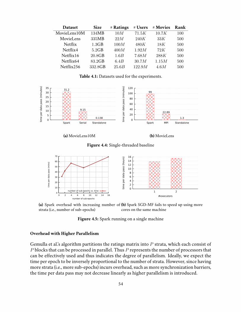
Dataset Size # Ratings # Users # Movies RankMovieLens10M 134MB 10M 71.5K 10.7K 100

MovieLens 335MB 22M 240K 33K 500

Netflix 1.3GB 100M 480K 18K 500

Netflix4 5.2GB 400M 1.92M 72K 500

Netflix16 20.8GB 1.6B 7.68M 288K 500

Netflix64 83.2GB 6.4B 30.7M 1.15M 500

Netflix256 332.8GB 25.6B 122.9M 4.6M 500

Table 4.1: Datasets used for the experiments.

0

5

10

15

20

25

30

35

Spark Serial Standalone

tim

e p

er

data

pass

(m

inute

s)

31.2

9.15

0.138

(a) MovieLens10M

0

20

40

60

80

100

120

Spark MPI Standaloneti

me p

er

data

pass

(m

inute

s)

99

22.89

1.3

(b) MovieLens

Figure 4.4: Single-threaded baseline

0

10

20

30

40

50

60

70

0 2 4 6 8 10 12 14 16

tim

e p

er

data

pass

(m

ins)

number of sub-epochs

number of sub-epochs vs. time

(a) Spark overhead with increasing number ofstrata (i.e., number of sub-epochs)

0

2

4

6

8

10

12

14

16

1 2

tim

e p

er

data

pass

(hours

)

#executors

(b) Spark SGD-MF fails to speed up using morecores on the same machine

Figure 4.5: Spark running on a single machine

Overhead with Higher Parallelism

Gemulla et al.’s algorithm partitions the ratings matrix into P strata, which each consist ofP blocks that can be processed in parallel. Thus P represents the number of processors thatcan be effectively used and thus indicates the degree of parallelism. Ideally, we expect thetime per epoch to be inversely proportional to the number of strata. However, since havingmore strata (i.e., more sub-epochs) incurs overhead, such as more synchronization barriers,the time per data pass may not decrease linearly as higher parallelism is introduced.

54

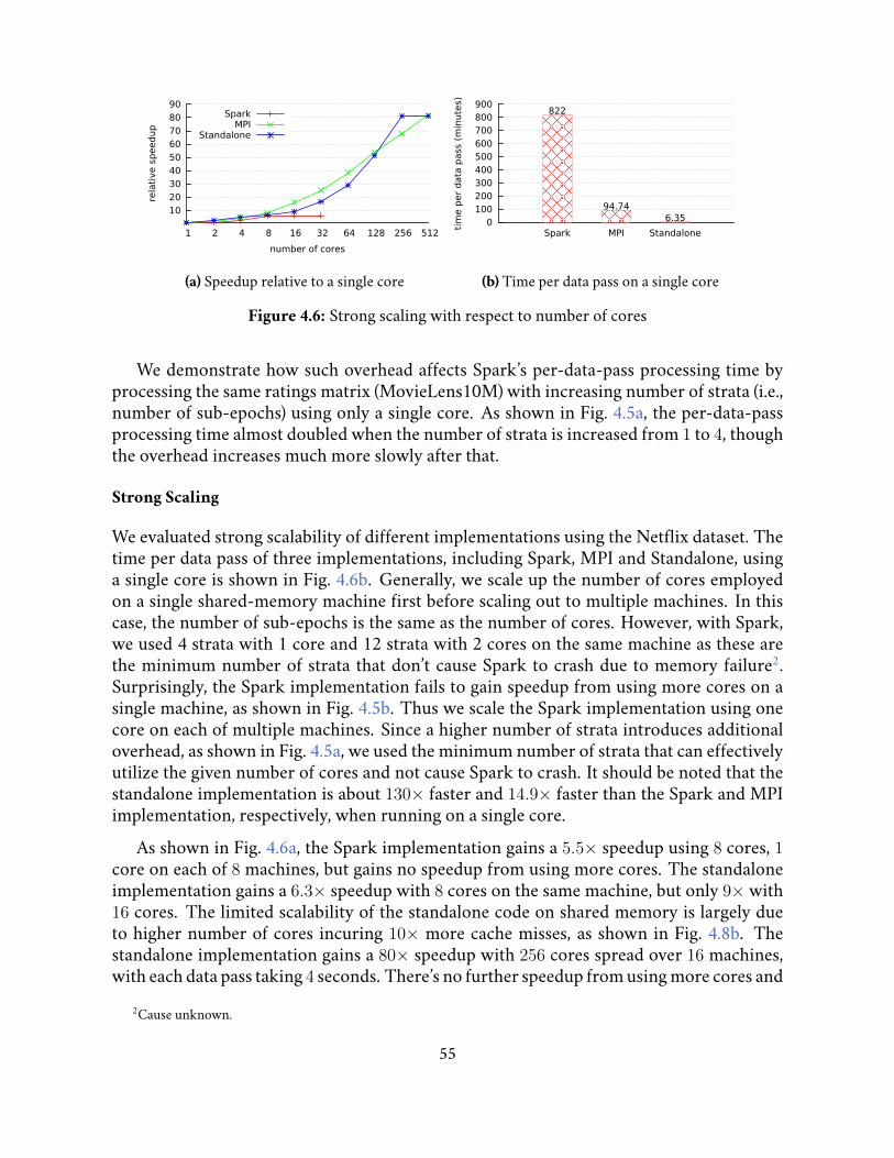
10 20 30 40 50 60 70 80 90

1 2 4 8 16 32 64 128 256 512

rela

tive s

peed

up

number of cores

SparkMPI

Standalone

(a) Speedup relative to a single core

0 100 200 300 400 500 600 700 800 900

Spark MPI Standalone

tim

e p

er

data

pass

(m

inute

s)

822

94.746.35

(b) Time per data pass on a single core

Figure 4.6: Strong scaling with respect to number of cores

We demonstrate how such overhead affects Spark’s per-data-pass processing time byprocessing the same ratings matrix (MovieLens10M) with increasing number of strata (i.e.,number of sub-epochs) using only a single core. As shown in Fig. 4.5a, the per-data-passprocessing time almost doubled when the number of strata is increased from 1 to 4, thoughthe overhead increases much more slowly after that.

Strong Scaling

We evaluated strong scalability of different implementations using the Netflix dataset. Thetime per data pass of three implementations, including Spark, MPI and Standalone, usinga single core is shown in Fig. 4.6b. Generally, we scale up the number of cores employedon a single shared-memory machine first before scaling out to multiple machines. In thiscase, the number of sub-epochs is the same as the number of cores. However, with Spark,we used 4 strata with 1 core and 12 strata with 2 cores on the same machine as these arethe minimum number of strata that don’t cause Spark to crash due to memory failure2.Surprisingly, the Spark implementation fails to gain speedup from using more cores on asingle machine, as shown in Fig. 4.5b. Thus we scale the Spark implementation using onecore on each of multiple machines. Since a higher number of strata introduces additionaloverhead, as shown in Fig. 4.5a, we used the minimum number of strata that can effectivelyutilize the given number of cores and not cause Spark to crash. It should be noted that thestandalone implementation is about 130× faster and 14.9× faster than the Spark and MPIimplementation, respectively, when running on a single core.

As shown in Fig. 4.6a, the Spark implementation gains a 5.5× speedup using 8 cores, 1core on each of 8 machines, but gains no speedup from using more cores. The standaloneimplementation gains a 6.3× speedup with 8 cores on the same machine, but only 9× with16 cores. The limited scalability of the standalone code on shared memory is largely dueto higher number of cores incuring 10× more cache misses, as shown in Fig. 4.8b. Thestandalone implementation gains a 80× speedup with 256 cores spread over 16 machines,with each data pass taking 4 seconds. There’s no further speedup from using more cores and

2Cause unknown.

55

5

10

15

20

25

1 2 4 8 16 32

rela

tive s

peed

up

number of machines

SparkMPI

StandaloneBosenStrads

(a) Speedup relative to a single 16-core machine

0

2

4

6

8

10

Spark MPI Bosen Strads Standalone

tim

e p

er

data

pass

(m

inute

s) 822

5.8

3.88

2.42

0.63

(b) Time per data pass on a single 16-core ma-chine

Figure 4.7: Strong scaling with respect to number of machines

most of the time is now spent on communication. The MPI implementation scales similarlyto the standalone implementation.

Strong scalability with respect to the number of machines and a comparison with twogeneral-purpose ML systems Bosen and STRADS is shown in Fig. 4.7a, and the time perdata pass with different implementations running on a single machine (Spark uses only 1core) is shown in Fig. 4.7b.

The Bosen implementation runs slower than the standalone implementation on a shared-memory multi-core machine as the Bosen client library employs locking for concurrencycontrol and uses the adaptive gradient method [110] that incurs high computation over-head than plain SGD. While STRADS (also using adaptive gradient) scales better than thestandalone implementation, the standalone implementation still faster with less resources,achieving about 4 seconds per data pass with 16 machines and STRADS achieves 6 secondsper data pass with 64 machines (no further speedup with more machines for both imple-mentations).

Weak Scaling

We evaluated the weak scalability of the standalone implementation using the Netflix datasetduplicated a number of times propotional to the number of cores. 8 cores were assigned forthe original Netflix data; 32 cores, i.e., 2 Nome nodes, were assigned for 4× Netflix data;etc. With weak scaling, we double work (training dataset size) when we double resourcesand hope for execution time per epoch to remain fixed, representing linear weak scaling.While the time per data pass remains roughly unchanged up to 16×duplicated data, with thenumber of cores proportionally increasing, it increased considerably for the 64× and 256×duplicated datasets. Even the most optimized standalone implementation cannot linearlyscale to larger datasets.

We failed to run the Spark implementation on even 4× duplicated Netflix data due toconsistent executor-lost failure during the first data pass. No hardware failure was ob-served.

56

0

500

1000

1500

2000

2500

1 4 16 64 256time

per d

ata

pass

(min

utes

)

relative data size

near linear scalingpoor sc

aling

(a)Weak scaling of pipelined standalone Gemullaet al.’s SGD MF with respect to number of cores(up to 2048 cores)

1 2 3 4 5 6 7 8 9

10 11

1 2 4 8 16norm

aliz

ed

tota

l ca

che m

isse

s

number of cores

normalized total cache misses

(b) Normalized cache misses w/ the standaloneimplementation

Figure 4.8: Weak scaling and cache misses

4.2.5 Discussion

Spark’s ease of programming comes at a high performance degradation. The immutabilityof RDD makes it easy to parallelize the DAG computation and achieve fault tolerance. How-ever, The rigrid map-reduce execution model makes it impossible to implement the highlycustomized pipelining communication. The lack of random reads and in-place updates onRDDs restricts parameter updates to be performed by inefficient RDD joins or non-scalablebroadcast.

The standalone pipelining implementation achieves best efficiency, i.e., achieving high-est throughput using least amount of resources, but requires high programmer effort toimplement inter-machine communication, worker coordination, etc. Machine learningframeworks such as STRADS and Bosen achieve high throughput and efficiency that’s closeto the standalone implementation and substantially reduces programmer effort by abstract-ing away many system details, such as network communication, parameter caching, etc butstill requires non-trivial manual parallelization effort, especially when implementing a par-allel computation schedule that’s more complex than data parallelism.

4.3 Summary

Manually parallelized machine learning programs such as LightLDA on Bosen and SGDMF, including standalone implementation and implementations on STRADS and Bosenachieves high performance but require substantial programmer effort. Thanks to its higherlevel of abstraction, Spark indeed greatly simplifies application development compared tomaunal parallelization (a few days vs. a couple of weeks or even months), but the experi-mental evaluation suggests that Sparks suffers major performance penalty.

We desire a framework that provides an appropriate higher-level abstraction than STRADS’and Bosen’s to simplify machine learning application development while achieves highly ef-ficient execution. A good high-level abstraction captures the key characteristics of the appli-

57

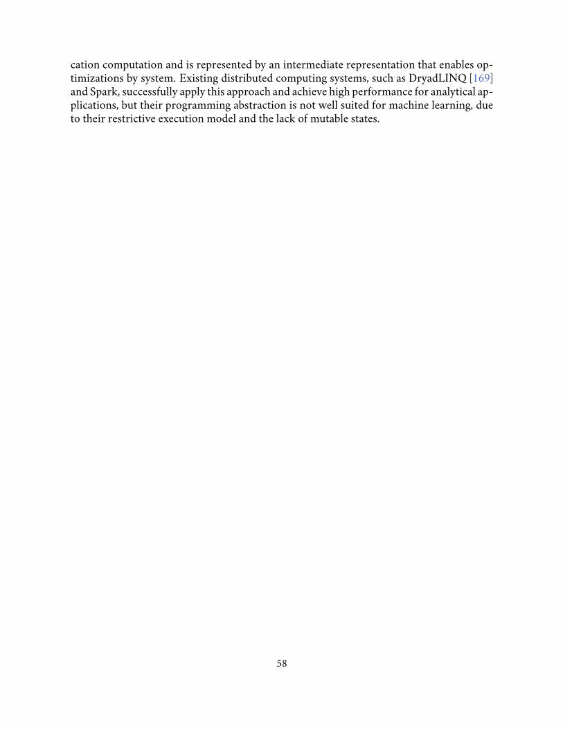
cation computation and is represented by an intermediate representation that enables op-timizations by system. Existing distributed computing systems, such as DryadLINQ [169]and Spark, successfully apply this approach and achieve high performance for analytical ap-plications, but their programming abstraction is not well suited for machine learning, dueto their restrictive execution model and the lack of mutable states.

58

Chapter 5

SchedulingComputationviaAutomaticParalleliza-tion

While parallelization that preserves a serial algorithm’s data dependence improves the learn-ing algorithm’s convergence rate, it requires substantial programmer effort to manuallyanalyze data dependence and implement efficient distributed programs. Moreover, vio-lating minor data dependence may increase the degree of parallelism with negligible im-pact on convergence rate. Such opportunities requires domain knowledge of the applica-tion program to explore. In this chapter, we present a holistic approach for automatingdependence-aware parallelization and its implementation – Orion. Orion’s programmingmodel and system abstraction natively support frequently mutated states and capture theaccess pattern on mutable states for parallelization. In this way, Orion substantially reducesprogrammer effort while achieving competitive performance compared to state-of-the-artmanual parallelization.

5.1 Dependence-aware Parallelization

Given a training dataset D = {Di|1 ≤ i ≤ N} where Di denotes a mini-batch of one ormultiple data samples, a serial training algorithm computes an update function ∆ (At,Di)for each mini-batch Di using the current parameter values At and updates the parametersbefore processing the next mini-batch. Note that some ML algorithms update model pa-rameters after processing each data sample, which is a special case that has a mini-batchsize of 1. With an application-defined mini-batch size, our discussion is focused on thedependence across mini-batches.

Training algorithms typically take many passes (i.e., iterations) over the training datasetbefore they converge. In many ML applications, ∆ reads only a subset of the model pa-rameters and generates refinements to a (possibly different) subset of parameters. If eachworker is assigned with a mini-batchD′k such that the read-write sets of all ∆ (At,D′k) com-putations are disjoint, then the parallel execution of multiple mini-batch computation isserializable. That is, the parallel execution produces the same result as a serial exeuctionfollowing some sequential ordering of the mini-batches. We refer to this style of paral-

59

R/WD1 a1 a3

D2 a1 a4

D3 a2 a3

D4 a2 a4

(a) Read-write sets

a1 a2 a3 a4

D1 D2

sync barrierD3 D4

W1, ∆ W2, ∆

(b) Data parallelism

a1 a2 a3 a4

D1 D4

sync barrierD2 D3

W1, ∆ W2, ∆

(c) Dep-aware

Figure 5.1: Data parallelism vs. dependence-aware parallelism: (a) the read-write (R/W) sets ofdata mini-batchesD1 toD4; (b) in data parallelism, mini-batches are randomly assigned to workers,leading to conflicting parameter accesses; (c) in dependence-aware parallelization (note that D4 in-stead of D2 is scheduled to run in parallel with D1), mini-batches are carefully scheduled to avoidconflicting parameter accesses.

lelization that preserves data dependence among mini-batches as dependence-aware paral-lelization. Fig. 5.1 compares data parallelism with dependence-aware parallelism. Notethat under the dependence-aware parallelization shown, the parallel execution is equiva-lent to sequentially processing mini-batches D1, D4, D2, and D3 (serializable), while underthe shown data-parallelism, execution is not serializable.

STRADS 1 [90] is a scheduler framework for traditional model-parallel ML programs. Itexploits independent parameter access from different data samples to achieve state-of-the-art convergence rate for SGD MF and topic modeling (LDA), which is considerably fastercompared to data parallelism when such parallelization is applicable. However, STRADSrequires programmers to manually parallelize the training algorithm, which demands sig-nificant programmer effort and is error-prone.

Generally, with manual parallelization, programmers identify the data dependences amongloop iterations based on how they access shared memory and devise a computation sched-ule. A computation schedule breaks down the iteration space (e.g., Z) into partitions, whichconceptually form a dependency graph. An ideal partitioning provides sufficient parallelism(i.e., many partitions can be executed in parallel) while amortizing synchronization over-head (i.e., partitions are large enough). The computation schedule also assigns partitionsto workers. Dependencies among iteration space partitions incur synchronization amongworkers and network communication. Partition assignment affects synchronization fre-quency and communication volume.

In contrast, our system Orion automates dependence-aware parallelization of serial im-perative ML programs for efficient distributed execution. Orion’s parallelization strategiesare similar to STRADS but our focus is on automating dependence analysis and dependence-aware parallelization for serial imperative ML programs. Compared to Orion, STRADSperforms neither static or dynamic analysis, nor code generation. Application programmers

1STRADS is open-sourced here: https://github.com/sailing-pmls/strads (last visited: 1/10/2019). SGD MF isnot part of the open-sourced repository and was obtained from STRADS authors.

60

Orion Master

Orion Worker

Orion Worker

Orion Worker

Driver Program

DistArray

DistArray

DistArray

Figure 5.2: Orion System Overview

thus manually analyze data dependence and derive a computation schedule. While deriv-ing an efficient computation schedule is most challenging, implementation is also highlynon-trivial. SGD MF on STRADS is implemented as a coordinator and a worker program,totally consisting of 1788 lines of C++ code. The application program is responsible forcoordination among workers, data partitioning, parameter communication and synchro-nization, etc. Due to STRADS’ low-level abstraction, there may be little code reuse acrossSTRADS applications. STRADS-AP [91] simplifies application programming by perform-ing a “virtual iteration” that does dynamic analysis for dependences that do not change inlatter iterations.

While imperative programming with a shared memory abstraction is highly expressiveand natural for programmers, parallelization is more difficult compared to functional pro-gramming as dependency has to be inferred from memory accesses. Orion employs staticdependence analysis and parallelization techniques from automatic parallelizing compilersand takes advantage of ML-specific properties to relax program semantics and thus im-prove parallelism. Sematic relaxations include programmer-controlled dependence viola-tion, which enables data parallelism with few code changes. Orion’s programming modelabstracts away worker coordination by providing high-level primitives such as@parallel_for, map and groupBy. Moreover, Orion generates code for data loading, partitioning, andprefetching, tailored to specific data types, so that a computation schedule can be resued fordifferent computation and data types without losing efficiency. Thus application program-mers can focus on the core ML algorithm. Moreover, Orion minimizes remote randomaccess overhead via automated data partitioning and bulk prefetching based on the mem-ory access pattern discovered in static analysis to achieve efficient distributed execution.

Experiments on a number of ML applications confirm that preserving data dependencecan significantly improve ML training’s convergence progress and our proposed techniquesare effective. We also compare Orion with various offline ML training systems [16, 90, 157]and show that Orion achieves much better or matching convergence progress and at leastcomparable computation throughput, even when compared with state-of-the-art manualparallelization, while substantially reducing programmer effort.

61

5.2 Orion ProgrammingModel

Orion consists of a distributed runtime and an application library (Fig 5.2). Orion appli-cation programmers implement an imperative driver program that executes instructionslocally and in Orion’s distributed runtime using the application library. Distributed pro-gramming in Orion seamlessly integrates with the rest of the program thanks to Orion’sdistributed shared memory (DSM) abstraction and parallel for-loops. Our prototype imple-mentation supports application programs written in Julia [24]. Julia is a scripting languagethat offers high programmer productivity like Python with great execution speed [6] usingjust-in-time compilation.

5.2.1 Distributed Arrays

Orion’s main abstraction for DSM is a set of multi-dimensional matrices, which we refer toas Distributed Arrays (or DistArrays). A DistArray can contain elements of any serializabletype and may be either dense or sparse. A DistArray is partitioned and stored in the memoryof a set of distributed machines in Orion’s runtime and Orion automatically repartitionsDistArrays to minimize remote access overhead when executing distributed parallel for-loops.

Elements of an N-dimensional DistArray are indexed with an N-tuple (p1, p2, ..., pn).A DistArray supports random access via both point queries (e.g., A[1, 3, 2]) to access asingle element and set queries (e.g., A[1:3, 3, 2]) where a range is specified for one ormultiple DistArray dimensions. Here [1, 3, 2] and [1:3, 3, 2] are DistArray subscripts,analogous to DSM addresses. Statements that access DistArray elements can either executelocally or in Orion’s distributed workers by using the parallel for-loop primitive.

Similar to Resilient Distributed Datasets (RDD) [174], DistArrays can be created by load-ing from text files using a user-defined parser or by transforming an existing DistArray us-ing operations like map and groupBy. Text file loading and map operations are recorded byOrion and not evaluated until the driver program calls materialize. This allows Orionto fuse the user-defined functions across operations and avoids memory allocation for in-termediate results. Unlike RDDs, set operations that may cause shuffling, such as groupBy,are evaluated eagerly for simplicity. We expect the performance impact of this simplicationto be small for machine learning programs as the heavy computation happens in for-loopsand is parallelized using parallel for loop (Sec. 5.2.2).

Compared to RDD, DistArray supports indexed random accesses (i.e., point and setqueries) and in-place updates, which makes DistArray better suited for holding trainablemodel parameters which are iteratively updated, especially when each mini-batch updatesonly a subset of the parameters. A DistArray is automatically distributed among a set ofworker machines and can be sparse. At the lowest level, TensorFlow tensors are dense ma-trices that reside on a single device and TensorFlow applications may manually representsparse and distributed matrices using dense tensors (e.g., [136]). While DistArray does notprovide a rich set of linear algebra operations like TensorFlow tensors, a DistArray set query

62

1 Orion.@parallel_for for (e_idx, e_val) in A

2 ...loop body...

3 end

Figure 5.3: Distributed parallel for-loop example

returns a Julia Array, which can leverage the rich set of linear algebra operations nativelyprovided by Julia.

5.2.2 Distributed Parallel For-Loop

The driver program may iterate over the elements of an N-dimensional DistArray using avanilla Julia for-loop. For example, the loop in Fig. 5.3 iterates over each element of Dis-tArray A where e_idx is the element’s index and e_val is the element’s value. As A is aN-dimensional matrix, the for-loop is naturally an N-level perfectly nested loop and theDistArray represents the loop nest’s iteration space. Each DistArray element corresponds toa loop iteration and the element’s index e_idx is the loop iteration’s index vector, of whicheach element is referred to as a loop index variable.

For-loops iterating over a DistArray can be parallelized across a set of distributed work-ers using a @parallel_for macro. Depending on the loop body’s access pattern to otherDistArrays, parallelization assigns iterations to workers and adds synchronization whenit is needed for preserving data dependence among loop iterations (i.e., loop-carried de-pendence). Iterations that have dependences between them because of shared accesses onDistArrays 2 are executed one after another in the correct order. Thus the parallel executionis equivalent to a serial execution of the loop (serializable).

Tools like OpenMP [48] and MATLAB parfor [7] also provide parallel for-loop primi-tives, provided that the programmer asserts the for-loops have no dependency among its it-erations. But Orion’s @parallel_formacro can be applied to loops that have dependencesamong iterations, and preserves loop-carried dependences. Moreover, Orion’s parallel for-loop executes in a distributed cluster while existing tools only apply to single machines.

Let P = {(p1, p2, ..., pn)|∀i ∈ [1, n] : 0 ≤ pi < si} represent the iteration space of a n-dimensional DistArray, where (p1, p2, ..., pn) represents the index vector of an iteration, andthe size of the iteration space’s i-th dimension is si. For any two iterations ~p = (p1, p2, ..., pn)and ~p′ = (p′1, p

′2, ..., p

′n), Orion can parallelize the for-loop while preserving all loop-carried

dependences if one of the following is true:

1. 1D Parallelization: There exists a dimension i such that when pi 6= p′i, there doesn’texist any loop-carried dependence between iteration ~p and iteration ~p′. Note that thisalso includes the case when there’s no dependence between any iterations.

2. 2D Parallelization: There exist two dimensions i and j such that when pi 6= p′i and2They both access the same DistArray element and at least one of the accesses is a write.

63

pj 6= p′j , there doesn’t exist any loop-carried dependence between iteration ~p and iter-ation ~p′.

3. 2D Parallelization w/ Unimodular Transformation: When neither 1D nor 2Dparallelization is applicable, in some cases (see Sec. 5.3.3), unimodular transforma-tions [159] may be applied to transform the iteration space to enable 2D paralleliza-tion.

Applicability. Static parallelization requires the size of the iteration space to be constantand known at compile time. ML training applications usually iterate over a fixed data setor model parameters and Orion just-in-time compiles a for-loop after the iteration spaceDistArray is loaded or created. Orion’s dependence-aware parallelization strategies applyto for-loops when the loop body accesses only a subset of the shared memory addresses andthe addresses can be fully determined given the loop index variables, i.e., the iteration-spaceDistArray index. More specifically, our current implementation accurately captures depen-dence when DistArray subscripts contain at most one loop index variable plus or minus aconstant at each position. A more complex subscript is conservatively regarded as that itmay take any value within the DistArray’s bounds. The loop body may inherit any driverprogram variable. The inherited variables are assumed to be read-only 3 during a single loopexecution but their values could change between different executions of the same loop.

ML applications commonly represent data records as a mapping from a n-tuple key toa value, i.e., (k_1, k_2, ..., k_n)→ value, where the key uniquely identifies the datarecord. Thus data records may be organized in a n-dimensional tensor, indexed by the keytuple. When parameter accesses are also indexed by the key tuple, parallelization via staticdependence analysis is possible. For example, the popular bag-of-words model representstext as a set of mappings from a word to its number of occurrences. ML applications on textdata often have parameters associated with each word, such as the word topic count vectorin topic modeling with Latent Dirichlet Allocation or the word embedding vector, whichare accessed based on word ID.

Deep neural network (DNN) training is an increasingly important class of ML work-loads. The core computation of a typical DNN training program is a loop that iterates overdata mini-batches where each iteration performs a forward pass, a backward pass and up-dates the neural network weights. DNNs commonly read and update all weights in eachiteration, therefore serializable parallelization over mini-batches is not applicable. DNNtraining is most commonly parallelized with data parallelism, which can be achieved inOrion by permitting dependence violation as discussed in Sec. 5.2.3.

5.2.3 Distributed Array Buffers

Static dependence analysis avoids materializing a huge dependence graph whose size ispropotional to the training dataset. Such a graph could be too expensive to store and an-

3The loop body may still write to those variables but the new value is visible only to the worker that performs thewrite.

64

alyze. However, static dependence analysis requires the DistArray subscripts to be deter-mined (as an expression of loop index variables and constants) statically to accurately cap-ture the dependence among loop iterations.

First, some ML models, such as DNNs, perform dense parameter accesses. Second,while parameter accesses might be sparse in some models, the DistArray subscripts maydepend on runtime values (e.g., e_val in Fig. 5.3). For example, in sparse logsitic regres-sion, processing a data sample reads and updates the weights corresponding to the sam-ple’s nonzero features. In this case, traditional dependence analysis conservatively marksall DistArray positions as accessed, leading to false dependences among iterations and im-peding parallelization. For these models, serializable parallelization can be severely limitedin computation throughput or simply inapplicable, therefore such ML training applicationsare often parallelized with dependence violations. The algorithm converges better (closerto serial execution) when there are fewer collisions and when writes make small changes.In order to support these applications, Orion application programmers may selectively ex-empt certain (or all) writes from dependence analysis using Distributed Array Buffers (orDistArray Buffers). By applying all writes to DistArray Buffers instead of DistArrays, anOrion application effectively resorts to data parallelism.

A DistArray Buffer is a write-back buffer of a DistArray, and provides the same API forpoint and set queries. A DistArray Buffer maintains a buffer instance on each worker, whichis usually initialized empty. The application program may apply a subset of DistArray writesto a corresponding DistArray Buffer and exempt those writes from dependence analysis,making it possible to parallelize a for-loop that can’t be parallelized otherwise.

Typically the buffered writes are applied to the corresponding DistArray after the workerexecutes multiple for-loop iterations. The application program may optionally bound howlong the writes can be buffered. Orion supports an element-wise user-defined function(UDF) for applying each DistArray Buffer’s buffered writes. This UDF is executed atomi-cally on each DistArray element and thus supports atomic read-modify-writes. The UDFfor applying buffered writes allows applications to define sophisticated custom logic for ap-plying updates, and makes it easy to implement various adaptive gradient algorithms [54,110, 142].

5.2.4 Putting Everything Together

Fig. 5.4 shows a Julia SGD MF program parallelized by Orion. The serial program has lessthan 90 lines of Julia code and can be parallelized by changing only a few lines. The parallelprogram creates DistArrays instead of local matrices for training data (ratings) and param-eters (W and H) by loading from text files (text_file) or random initialization (randomn).DistArrays can be manipulated with set operations, like map (e.g., line #9). The for-loopsthat iterate over the ratingsmatrix entries (e.g., line #14) are parallelized by applying the@parallel_formacro.

The parallel for-loop’s loop body may read any driver program variable that is visible

65

1 step_size = 0.01

2 # Omitted variable and function definitions

3 Orion.@dist_array ratings =

4 Orion.text_file(data_path , parse_line)

5 Orion.materialize(ratings)

6 dim_x, dim_y = size(ratings)

7 Orion.@dist_array W = Orion.randn(K, dim_x)

8 Orion.@dist_array W = Orion.map(W, init_param , map_values=true)

9 Orion.materialize(W)

10 Orion.@dist_array H = Orion.randn(K, dim_y)

11 Orion.@dist_array H = Orion.map(H, init_param , map_values=true)

12 Orion.materialize(H)

13 Orion.@accumulator err = Float32(0.0)

14 for iter = 1:num_iterations

15 Orion.@parallel_for for (key, rv) in ratings

16 W_row = @view W[:, key[1]]

17 H_row = @view H[:, key[2]]

18 pred = dot(W_row, H_row)

19 W_grad .= -2 * (rv - pred) * H_row

20 H_grad .= -2 * (rv - pred) * W_row

21 W[:, key[1]] .= W_row - W_grad * step_size

22 H[:, key[2]] .= H_row - H_grad * step_size

23 end

24 Orion.@parallel_for for (key, rv) in ratings

25 pred = dot(W_row, H_row)

26 err += abs2(rv - pred)

27 end

28 err = Orion.get_aggregated_value(:err, :+)

29 Orion.reset_accumulator(:err)

30 end

Figure 5.4: SGD Matrix Factorization Parallelized using Orion

66

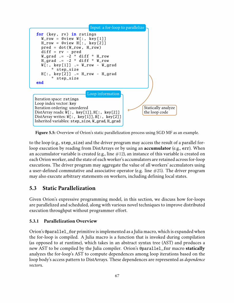
for (key, rv) in ratingsW_row = @view W[:, key[1]]H_row = @view H[:, key[2]]pred = dot(W_row, H_row)diff = rv - predW_grad .= -2 * diff * H_rowH_grad .= -2 * diff * W_rowW[:, key[1]] .= W_row - W_grad

* step_sizeH[:, key[2]] .= H_row - H_grad

* step_sizeend

Input: a for-loop to parallelize

Iteration space: ratingsLoop index vector: keyIteration ordering: unorderedDistArray reads: W[:, key[1]], H[:, key[2]]DistArray writes: W[:, key[1]], H[:, key[2]]Inherited variables: step_size, W_grad, H_grad

Loop information

Statically analyzethe loop code

Figure 5.5: Overview of Orion’s static parallelization process using SGD MF as an example.

to the loop (e.g., step_size) and the driver program may access the result of a parallel for-loop execution by reading from DistArrays or by using an accumulator (e.g., err). Whenan accumulator variable is created (e.g., line #12), an instance of this variable is created oneach Orion worker, and the state of each worker’s accumulators are retained across for-loopexecutions. The driver program may aggregate the value of all workers’ accmulators usinga user-defined commutative and associative operator (e.g. line #25). The driver programmay also execute arbitrary statements on workers, including defining local states.

5.3 Static Parallelization

Given Orion’s expressive programming model, in this section, we discuss how for-loopsare parallelized and scheduled, along with various novel techniques to improve distributedexecution throughput without programmer effort.

5.3.1 Parallelization Overview

Orion’s @parallel_for primitive is implemented as a Julia macro, which is expanded whenthe for-loop is compiled. A Julia macro is a function that is invoked during compilation(as opposed to at runtime), which takes in an abstract syntax tree (AST) and produces anew AST to be compiled by the Julia compiler. Orion’s @parallel_for macro staticallyanalyzes the for-loop’s AST to compute dependences among loop iterations based on theloop body’s access pattern to DistArrays. These dependences are represented as dependencevectors.

67

∀ iterations ~p = (p1, p2), ~p′ = (p′1, p′2) and

~p′ > ~p, ~p′ depends on ~p if(:, p1) == (:, p′1) or (:, p2) == (:, p′2), i.e.,{

:=:

p1 = p′1or{

:=:

p2 = p′2. The dependence

vecotrs are thus (0,∞) and (∞, 0).

Compute dependence vectors (Sec. 4.2)

Since ∀ dependence vector ~d = (d1, d2), d1 = 0or d2 = 0, unordered 2D parallelization isapplicable. Partition ratings by its 1st and2nd dimension.

Partition & schedule the iteration space (Sec. 4.3)

W and H are range partitioned by its 2nd di-mension and allocated among executors. Thesmaller one of W and H is rotated amongexecutors.

Partition accessed DistArrays (Sec. 4.4)

Compilation process:

Statically extract loop information

Compute dependence vectors

Determine the iteration space’spartitioning scheme and computa-tion schedule

Determine the accessed DistAr-rays’s partitioning scheme

Code generation: DistArray parti-tioning, driver variable broadcast,loop body functions, parallel for-loop execution, etc.

Figure 5.6: Overview of Orion’s static parallelization process using SGD MF as an example.

Based on the dependence pattern, Orion decides whether the for-loop is 1D or 2D paral-lelized and whether a unimodular transformation is needed (see Sec. 5.3.3). During macroexpansion, Orion generates functions that perform the loop body’s computation and de-fines those functions in the distributed workers. According to the parallelization strategy,the generated new AST, that executes on driver, invokes a static computation schedule withthe corresponding loop body functions. The generated AST also contains code that 1) repar-titions relevant DistArrays to minimize remote access overhead; and 2) captures and broad-casts driver program variables that are inherited in the loop body’s scope. Note that eventhough the parallel for-loop may itself be inside of another for-loop and executed multipletimes, the macro expansion and compilation is executed only once. A global statement in aJulia program is just-in-time compiled and executed before the following global statementsare compiled. Thus the compilation of a statement may make use of previous statements’runtime execution results, such as DistArray sizes. Fig. 5.6 presents an overview of the JITcompilation process using SGD MF as an example.

5.3.2 Computing Dependence Vectors

A lexicographically positive vector4 ~d denotes a dependence vector of an n-loop nest if andonly if there exist two dependent iterations ~p1 and ~p2 such that ~p1 = ~p2 + ~d. Infinity ∞

4A vector ~d = (d1, d2, ..., dn) is lexicographically positive if ∃i : di > 0 and ∀j < i : dj ≥ 0

68

Algorithm 3: Computing dependence vectorsinput : refs - the list of references on DistArray Doutput: dvecs - the set of dependence vectors due to references to Ddvecs = EmptySet();for each unique pair ref_a and ref_b in refs do

. Skip checking dependence if both references are read or if the loop is unordered and bothreferences are write.if (ref_a.is_read and ref_b.is_read) or(unordered_loop and ref_a.is_write and ref_b.is_write) then

continue;dvec = Vec(iter_space.num_dims, inf);independent = false;for dim ∈ D.dims dosub_a = ref_a.subs[dim];sub_b = ref_b.subs[dim];if sub_a and sub_b contains a single loop index variable then

if sub_a.dim_idx == sub_b.dim_idx thendist = sub_a.const - sub_b.const;if dvec[sub_a.dim_idx] != inf and dvec[sub_a.dim_idx] != dist thenindependent = true;break;

dvec[sub_a.dim_idx] = dist;else

continue;else

Test dependence for other subscript types;

if not independent thencorrect dvec for lexicographical positiveness;dvecs = union(dvecs, {dvec});

69

(or positive/negative infinity, +∞/−∞) in dependence vectors means that the dependencevector may take any (positive or negative) integer value at that position. In Fig. 5.6, depen-dence vector (0,∞) means that any iteration (p′1, p

′2) depends on iteration (p1, p2) as long as

p′1 − p1 == 0. A dependence vector implies a dependence pattern shared by all iterations,yielding a concise dependence representation. However, dependence vectors may conser-vatively represent a dependence that exists for only certain iterations as a dependence forall iterations, unnecessarily limiting parallelism.

Many previous work discussed how to compute dependence vectors [88, 108]. An iter-ation depends on another (earlier) iteration if and only if they both access the same mem-ory location and at least one of the accesses is a write. In general, computing dependencevectors requires performing a dependence test on the subscripts of each pair of DistArrayreferences from two different iterations, and either prove independence or produce a de-pendence vector for the loop indices occuring in the scripts [88]. Since Orion currentlysupports accurate dependence capturing only for subscripts that contain at most one loopindex variable plus or minus a constant at each position, we can simplify the algorithm. Werepresent each subscript as a 3-tuple (dim_idx, const, stype), representing the loopindex variable’s dimension index in the iteration space, the constant and the type of thesubscript, i.e., whether it is a single value or a range and whether the subscript is supportedfor dependence analysis. Alg. 3 presents Orion’s core procedure for computing dependencevectors. Our algorithm produces at most one dependence vector from each pair of staticDistArray references. Two DistArray references are independent when they are both read,and write-write dependence may be omitted when the loop iterations can be executed inany order (unordered_loop). After skipping such reference pairs, we initialize a depen-dence vector whose elements are infinity, meaning that any two iterations may be depen-dent due to these two DistArray references. We then refine this conservative dependenceby checking each subscript position. We declare the two references are independent if theirsubscripts will never match. In the end, we add the dependence vector to the set of depen-dence vectors after making sure it is lexicographically positive. The algorithm has a timecomplexity of O(N2 × D) for each referenced DistArray where N is the number of staticDistArray references and D is the number of dimensions of the referenced DistArray.

5.3.3 Parallelization and Scheduling

Orion partitions the iteration space based on dependence vectors so that different partitionscan be executed in parallel. Each worker is assigned a number of iteration space partitionsand synchronizes at most once per partition.

Figs. 5.7 through 5.12 show different parallelization strategies for a 4×4 iteration space,depending on the dependence pattern between iterations. Ellipses denote loop iterationsand edges denote dependence between iterations. Note that representing the dependence in(a) requires only 1 depenence vector, namely (0, 1), and representing the dependence in (b)and (c) requires only 2 dependence vectors, namely (1, 0) and (0, 1). Iterations of the samecolor are executed in parallel. Rectangles denote iteration space partitions. Workers are

70

j

i

(0, 0)(0, 1)(0, 2)(0, 3)

(1, 0)(1, 1)(1, 2)(1, 3)

(2, 0)(2, 1)(2, 2)(2, 3)

(3, 0)(3, 1)(3, 2)(3, 3)

w0 w1 w2 w3

Figure 5.7: 1D parallelization.

in_parallel for j = 0:(N-1)

for iter in partition[j]

execute_iteration(iter)

synchronize()

Figure 5.8: 1D computation schedule.

denoted as w0, w1, etc. M and N denote the number of unique time-dimension (vertical) andspace-dimension (horizontal) indices. I and J denote the length of the time and space di-mensions and m = M / I, n = N / J. Although it’s not shown here, typically each workeris assigned with multiple space-dimension indices for better load balancing and multipletime-dimension indices for pipelined parallelism (Sec. 5.3.4).

Given the set of dependence vectors D, if there exists a dimension i such that ∀~d =(d1, d2, ..., dn) ∈ D, di = 0, then any two iterations ~p = (p1, p2, ..., pn) and ~p′ = (p′1, p

′2, ..., p

′n)

are independent as long as pi 6= p′i. Partitioning the iteration space by dimension i ensuresthat any two iterations ~p and ~p′ from two different partitions are independent. Thus theloop can be scheduled by assigning different iteration space partitions to different work-ers as there’s no data dependence across partitions. This is referred to as 1-dimensional(i.e. 1D) parallelization. Note that all such dimensions i that satisfy the above conditionare candidate partitioning dimensions. Fig. 5.7 shows an example that applies 1D paral-lelization to a 2-level loop nest and partitions the 2D iteration space by dimension j. Thecorresponding compute schedule is shown in Fig. 5.8. The workers synchronize with eachother after executing all iterations in its assigned partition.

If there exist two dimensions i and j such that ∀~d = (d1, d2, ..., dn) ∈ D, di = 0, dj = 0,then any two iterations ~p = (p1, p2, ..., pn) and ~p′ = (p′1, p

′2, ..., p

′n) are independent as long

as pi 6= p′i and pj 6= p′j . In this case, the loop can be parallelized by partitioning the iterationspace by dimensions i and j, which we refer to as 2-dimensional (i.e. 2D) parallelization(see Fig. 5.9). The partitions are assigned to workers based on one of the dimensions, e.g.j in this case, which we refer to as the space dimension and the other dimension is referredto as the time dimension. The computation is executed in a sequence of global time steps.

71

j

i

(0, 0)(0, 1)(0, 2)(0, 3)

(1, 0)(1, 1)(1, 2)(1, 3)

(2, 0)(2, 1)(2, 2)(2, 3)

(3, 0)(3, 1)(3, 2)(3, 3)

w0 w1 w2 w3

Figure 5.9: 2D parallelization.

for time_step = 0:(M + N - 2)

in_parallel for j = 0:(N-1)

i = time_step - j

if i >= 0 && i < N

for iter in partition[j, i]

execute_iteration(iter)

synchronize()

Figure 5.10: 2D computation schedule.

j

i

(0, 0)(0, 1)(0, 2)(0, 3)

(1, 0)(1, 1)(1, 2)(1, 3)

(2, 0)(2, 1)(2, 2)(2, 3)

(3, 0)(3, 1)(3, 2)(3, 3)

w0 w1 w2 w3

Figure 5.11: Unordered 2D parallel.

for time_step = 0:(M-1)

in_parallel for j = 0:(N-1)

i = (j + time_step) % N

for iter in partition[j, i]

execute_iteration(iter)

synchronize()

Figure 5.12: Unordered 2D computation sched.

72

Within each time step, multiple workers may execute a local partition in parallel, wherethe partition’s time dimension index is derived from the time step number to ensure thatall parallel partitions’ indices differ in both space and time dimensions. We observe that apartition depends on only two other iteration space partitions from the previous time stepand one of them belongs to the same worker. Thus a worker waits for a signal from a singlepredecessor worker to begin the next time step instead of a global synchronization barrier.Relaxing the ordering constraints. Automatic parallelizing compiler preserves the lexi-cographical ordering of loop iterations and thus dependences indicate the execution order-ing of dependent loop iterations, such as shown in Fig. 5.9. With the ordering constraints,simultaneous execution of two iterations might not be possible even when they do not ac-cess the same memory location. For example, in Fig. 5.9, even though they do not access thesame memory location, iteration (3, 1) cannot be executed in parallel with (0, 0) due to theordering constraints enforced by iteration (3, 0).

Many ML algorithms, such as Gibbs sampling, do not require a particular ordering inwhich data samples or mini-batches are processed. Other algorithms such as stochasticgradient descent usually randomly shuffle the dataset before or during training. For suchML algorithms, even though different iteration ordering may result in different numericalvalues and thus affect convergence process. However, to our best knowledge, enforcing aparticular ordering, such as the lexicographical ordering, has not been shown to be ben-eficial while sacrificing parallelism. Therefore, Orion’s parallelization by default ensuresonly serializability but not the lexicogrpahical ordering. Application may enforce orderingby using the ordered argument in @parallel_for. Relaxing the ordering constraints al-lows Orion to reorder iterations to maximize parallelism: Orion schedules workers to startfrom different indices along the time dimension to fully utilize all workers (Fig. 5.11 andFig. 5.12).Unimodular transformation. When neither 1D or 2D parallelization can be directly ap-plied, Orion may apply unimodular transformations on the iteration space when the depen-dence vectors contain only numbers or positive infinity to enable 2D parallelization. Par-allelizing for-loops using unimodular transformations was introduced by Wolf et. al [159].The set of dependence vectors after unimodular transformation denoted as D′ satisfy that∀~d = (d1, d2, ..., dn) ∈ D′ : d1 > 0 (all dependences are carried by the outermost loop). Withthe transformed loop nest denoted asL1, L2, ...Ln, there’s no dependence between iterationsof the innermost loop nest L2, L3, ...Ln in the same outermost loop L1. Thus the for-loopcan be parallelized by partitioning the transformed iteration space by the outermost dimen-sion and any combination of the inner loop dimensions. By reversing the transformation,we can derive a 2D partitioning of the original iteration space.

As multiple candidate partitioning dimensions may exist, Orion uses a simple heuristicto choose the partitioning dimension(s) among candidates that minimizes the number ofDistArray elements needed to be communicated among Orion workers during loop execu-tion. This heuristic can be overridden by the application program.

73

D

D

D

D

(0, 0)01

(1, 2)23

(2, 4)45

(3, 6)67

(a) time step 0

(0, 1)1

(1, 3)3

(2, 5)5

(3, 7)7

0

4

2 6

(b) time step 1

(0, 2)2

(1, 4)4

(2, 6)5

(3, 0)0

1

5

3 7

(c) time step 2Figure 5.13: Pipelined computation of a 2D parallelized unordered loop on 4 workers. An el-lipse represents a worker executing a partition(space_partition_id, time_partition_id). Theworkers access different partitions of DistArrayD at different time steps. Partitions ofD that are beingused by workers are lime-colored and the partitions that are being communicated are pink-colored.At the beginning of the loop execution, each worker is assigned with 2 time partition indices andthus 2 partitions of DistArray D. Upon finishing the first time step, a worker sends out the updatedD partition and immediately begins the next time step using its locally available D partition.

DealingwithSkewedDataDistribution. As the parallel for-loop’s iteration space is oftensparse and the data distribution is often skewed, for example, when iterating over a skeweddataset, partitioning the iteration space into equal-sized partitions results in imbalancedworkload among workers. Orion DistArrays support a randomize operation that random-izes a DistArray along one or multiple dimensions to achieve a more uniform data distri-bution. Further more, Orion computes a histogram along each partitioning dimension toapproximate the data distribution, which is used to generate a more balanaced partitioning.Fault tolerance. An Orion driver program can checkpoint a DistArray by writing it todisk, which is eargerly evaluated. For ML training, a common approach is to checkpointthe parameter DistArrays every N data passes.

5.3.4 Reducing Remote Random Access Overhead

Generally, DistArray random access can be served by a parameter server. However, in thiscase, each random access potentially result in a remote access over the inter-machine net-work. The overhead of network communication is significant even when Orion workerscache DistArray values and buffer DistArray writes.Locality and pipelining. Usually different workers read and write to disjoint subsets ofelements of a DistArray. If the workers’ read/write sets are disjoint range partitions of aDistArray, the DistArray may be range partitioned among workers so random access to itcan be served locally.

Under 2D parallelization, the DistArray range partition accessed by a worker may bedifferent at different time steps and a worker has to wait to receive a DistArray partitionfrom its predecessor before starting a new time step. When the ordering constraints can be

74

Category Examples DSM Programming ParadigmDataflow Spark [174], DryadLINQ [169] No dataflow

Dataflow w/ mutable states TensorFlow [16] Yes dataflowParameter Server parameter server [100], Bosen [157] Yes imperativePS w/ scheduling STRADS [90] Yes imperativeGraph Processing PowerGraph [64], PowerLyra [31] Limited vertex programming

Orion Yes imperative

Table 5.1: Comparing different systems for offline machine learning training.

relaxed (Fig. 5.12), Orion avoids the workers’ idle waiting time by creating multiple time-dimension partition indices per worker and letting the worker proceed to a locally availabletime-dimension partition index while waiting for data from its predecessor, as illustratedin Fig. 5.13.Bulk prefetching. If the same elements of a DistArray are simultaneously accessed by dif-ferent workers, for example, when it is updated by a DistArray Buffer, or the disjoint setsof elements cannot be obtained from efficiently partitioning the DistArray, the DistArray isserved by a number of server processes, similar to a Parameter Server. In this case, in orderto minimize the random remote access overhead, Orion prefetches DistArray reads in bulk.

In order to accurately determine which values to prefetch, existing Parameter Serversystems rely on programmers to implement a “virtual iteration” besides the actual computa-tion to provide the parameter access pattern [45] or to manually implement prefetching andcache management [100]. Orion automates bulk prefetching by synthesizing a function thatgenerates the list of DistArray element indices that are read during the loop body computa-tion. The generated function executes loop body statements that read from non-locally allo-cated DistArrays, but instead of reading DistArray elements and performing computation,those statements are transformed to only record the DistArray subscript value. Since theDistArray subscripts may depend on runtime values, such as loop index variable and driverprogram variables (which are captured and broadcasted to workers as read-only variables),the function also executes statements that the DistArray subscripts have a data or controldependence on with proper control flow and ordering. If a DistArray subscript depends onvalues read from DistArrays, computing it may incur an expensive remote access. There-fore, DistArray subscripts that depend on other DistArray values are not recorded for bulkprefetching. The code generation algorithm is in spirit similar to dead code elimination.

5.4 Offline ML Training Systems: System Abstraction and API

In this section, we review and compare existing offline ML training systems (Table 5.1)with Orion, with an emphasis on their programming model and parallelization strategy.We focus on dataflow systems and graph processing systems, which present two distinctprogramming models.

75

5.4.1 Batch Dataflow Systems and TensorFlow

Many systems [16, 120, 169, 174] adopt a dataflow execution model, where the applicationprogram constructs a directed acyclic graph (DAG) that describes the computation and thecomputation DAG is lazily evaluated only when certain output is requested. A popular sys-tem among them is Spark [174], in which each node of the DAG represents a set of datarecords called a Resilient Distributed Dataset (RDD) and the edges represent transforma-tion operations that transform one RDD to another. A fundamental limitation of traditionaldataflow systems is that their computation DAG does not allow mutable states in order toensure deterministic execution, which makes updating model parameters an expensive op-eration. For example, mutable states in Spark such as driver local variables or accumulators,are not represented in the computation graph and are stored and updated by a single driverprocess. SparkNet [118] represents model weights as driver program local variables, whichare broadcasted to workers to compute new weights. The new weights produced by work-ers are collected and averaged by the driver. Each broadcast and collection takes about 20seconds.

TensorFlow [16] is a deep learning system which also adopts the dataflow programmingmodel, where nodes of the computation DAG represent operations whose inputs and out-puts are tensors flowing along the edges. TensorFlow introduces mutable states such as vari-able and queue into the computation graph to efficiently handle model parameter updates. Atypical TensorFlow program constructs a DAG that implements the update operation pro-cessing a single mini-batch of data, where trainable model parameters are represented asvariables. One approach to represent different mini-batch’s or data sample’s access patternon invidiudal model parameters is represent each mini-batch (or data sample) and modelparameter as separate nodes in the DAG (i.e., statically unroll the whole loop), resulting ina huge DAG that’s expensive to store and analyze.

Alternatively, the computation can be described as a while-loop [170] iterating overmini-batches or data samples. A TensorFlow application may parallelize a while-loop by as-signing different operations of the loop body to different computing devices, and differentdevices may compute operations from different iterations. While TensorFlow while-loopallows different iterations to be executed in parallel, each operation is still assigned withand bound to a single computing device. In other words, TensorFlow’s while loop doesnot partition its iteration space among distributed devices and may fail to exploit the fullparallelism enabled by the loop. On the other hand, TensorFlow while-loop enables addi-tional parallelism for loops with a large and complex loop body (e.g., a multi-layer RNN),since the loop body can be distributed among multiple computing devices. Moreover, Ten-sorFlow while-loop dynamically computes loop termination condition and supports data-dependent control flow inside the loop body including nested loops.

76

5.4.2 Graph Processing Systems

Graph processing systems [31, 64, 105, 106, 163, 176, 178] take a user-provided data graphas input and execute a vertex program on each graph vertex. Since a vertex program is re-stricted to access only data stored on that vertex itself, its edges or its neighboring vertices,the graph naturally describes the vertex program’s data dependence on mutable states. Thisproperty allows some systems to schedule independent vertex computation and ensure seri-alizability by using graph coloring or pessimistic concurrency control [64, 105, 106]. How-ever, graph coloring is an NP-complete problem and is expensive to perform; and withpessimistic concurrency control, lock contention may heavily limit the system’s scalabil-ity as demonstrated by a weak scaling experiment on PowerGraph [64]. As a result, re-cent graph processing systems have given up serializability: their vertex program eitherexecutes asynchronously or synchronizes with Bulk Synchronous Parallel synchroniza-tion [31, 163, 176, 178], both violating dependence among vertices.

5.5 Experimental Evaluation

Orion is implemented in ∼17, 000 lines of C++ and ∼6, 300 lines of Julia (v0.6.2). and hasbeen open sourced.5 In this section, we evaluate Orion, focusing on parallelization effec-tiveness and execution efficiency. Our experiments were conducted on a 42-node clusterwhere each machine contains an Intel E5-2698Bv3 Xeon CPU and 64GiB of memory. EachCPU contains 16 cores with hyper-threading. These machines are connected with 40GbpsEthernet.

5.5.1 Evaluation Setup andMethodology

We are interested in answering the following questions through experimental evaluation:

1. Is the traininng algorithms’ convergence rate sensitive to data dependence? Can de-pendence violation (such as data parallelism) significantly slow down algorithm con-vergence? Previous work (e.g., STRADS [90]) demonstrated that data dependence mayhave critical impact on algorithmic convergence and our results confirm their obser-vations.

2. Can proper semantic relaxations such as relaxing the loop ordering constraints andviolating non-critical dependences indeed improve computation throughput withoutjeopardizing convergence?

3. While preserving critical dependences, can Orion parallelization effectively speed upthe computation throughput and thus overall convergence rate of serial Julia ML pro-grams?

4. Do Orion applications achieve higher or competative computation throughput andconvergence rate compared to applications on other state-of-the-art offline ML train-ing systems, including both manually parallelized data- and model-parallel programs?

5URL: https://github.com/jinliangwei/orion

77

Acronym Model Learning Algorithm LoC ParallelizationsSGD MF Matrix Factorization SGD 87 2D Unordered

SGD MF AdaRev Matrix Factorization SGD w/ Adaptive Revision 108 2D UnorderedSLR Sparse Logistic Regression SGD 118 1D (data parallelism)

SLR AdaRev Sparse Logistic Regression SGD w/ Adaptive Revision 143 1D (data parallelism)LDA Latent Dirichlet Allocation Collaposed Gibbs Sampling 398 2D Unordered, 1DGBT Gradient Boosted Tree Gradient Boosting 695 1D

Table 5.2: ML applications parallelized by Orion.

ML applications. We’ve implemented a number of ML applications on Orion, exercisingdifferent parallelization strategies, as summarized in Table 5.2. In this section, we focus onevaluating performance for SGD MF (w/o and w/ AdaRev) and LDA, which are commonlyused benchmark applications and allow us to compare Orion with other systems.Datasets. We evaluated SGD MF (w/o and w/ AdaRev) on the Netflix dataset [1] for movierecommendation, which contains∼100 million movie ratings (rank is set to 1000). We eval-uated LDA on a smaller NYTimes dataset that contains ∼300 thousand documents and asubset of the large ClueWeb dataset [2] that contains∼25 million documents (32GB) (num-ber of topics is set to 1000 and 400 respectively).Metrics. Ultimately ML training applications desire to reach a high model quality in theleast amount of time, which we refer to as overall convergence rate. A high overall conver-gence rate requires the training system to both process a large number of data samples persecond, i.e., achieve a high computation throughput, and improve the model quality by a largemargin per data pass, i.e., achieve a high per-iteration convergence rate. A serial execution typ-ically achieves the best per-iteration convergence rate and thus serves as a golden standard.Different parallelizations may have different per-iteration convergence rate depending onwhether and which data dependences are violated. Our evaluation metrics include bothoverall and per-iteration convergence rate to properly attribute the performance difference.ML systems in compartion. We compared Orion with a number of state-of-the-art MLoffline training systems on SGD MF (w/ and w/o AdaRev) and LDA in terms of both com-putation throughput and overall convergence rate. The systems that we experimentallycompare to include Bosen parameter server [157], STRADS and TensorFlow.

TuX2 [163] is a recently proposed graph processing system, particularly optimized forML training workloads. TuX2 was reported to have over an order of magnitude faster per-iteration time on SGD MF compared to PowerGraph [64] and PowerLyra [31]. With a rankof 50, TuX2 SGD MF 6 takes∼0.7 seconds to perform one data pass on the Netflix dataset [1]using 8 machines, each with two Intel Xeon E5-2650 CPUs (16 physical cores), 256GiB ofmemory, and a Mellanox ConnectX-3 InfiniBand NIC with 54Gbps bandwidth (all higherthan ours except for slightly slower CPUs). In contrast, Orion SGD MF achieves a per-iteration time of∼1.4 seconds on 8 machines with the same number of CPU cores.

On the other hand, with a carefully tuned mini-batch size, TuX2 SGD MF reaches a6TuX2 is not open sourced

78

nonzero squared loss (lower is better) of ∼7 × 1010 in ∼600 seconds using 32 machines inits best case, while Orion SGD MF reaches ∼8.3 × 107 in ∼68 seconds using only 8 ma-chines. Even though TuX2 SGD MF achieves a higher computation throughput, its overallconvergence rate is much lower than Orion’s due to violating data dependence.

5.5.2 Summary of Evaluation Results

1. Preserving data dependence is critical for SGD MF (w/o and w/ AdaRev) and LDA.Dependence-violating parallelization (i.e., data parallelism) takes many more data passesthan serial execution to reach the same model quality, while dependence-aware paral-lelization (even with proper semantic relaxations) retains a comparable per-iteratoinconvergence rate to serial execution.

2. Orion-parallelized SGD MF (w/ and w/o AdaRev) and LDA converge significantlyfaster than manual data-parallel implementations on Bosen, in terms of both numberof iterations and wall clock time.

3. Data-parallel SGD MF AdaRev and LDA on Bosen converges faster with more fre-quent communication of parameter values and updates, approaching Orion paral-lelization at the cost of higher network bandwith.

4. Orion-parallelized SGD MF AdaRev and LDA achieve a matching per-iteration con-vergence rate to manual model-parallel programs on STRADS, but may have a slowertime per iteration mainly due to Julia’s language overhead compared to C++.

5. Orion-parallelized SGD MF converges considerably faster than a data-parallel imple-mentation on TensorFlow while achieving a 2.2× faster per-iteration time.

5.5.3 Parallelization Effectiveness

Application Ordered Unordered SpeedupSGD MF (Netflix) 13.1 5.9 2.2×

SGD MF AdaRev (Netflix) 43.6 16.7 2.6×LDA (NYTimes) 29.9 5.0 6.0×

Table 5.3: Time per iteration (seconds) with ordered and unordered 2D parallelization (12 ma-chines), averaged over iteration 2 to 100.

We compare Orion-parallelized Julia programs with serial Julia programs in terms ofboth computation throughput (i.e., time per iteration) and per-iteration convergence rate(Fig. 5.16). As shown in Fig. 5.14, although Orion abstraction incurs some overhead, Orionparallelization outperforms the serial Julia programs using only two workers and enablesconsistent speedup up to 384 workers. Although Orion’s parallelization relaxes the loop or-dering constrants for both SGD MF and LDA, and violates some non-critical dependencesin LDA, preserving (critical) dependences enable Orion parallelization to achieve a match-ing convergence rate to serial execution (Fig. 5.16a and Fig. 5.16b). On the other hand, dataparallelism (using Bosen) converges substantially slower than serial execution due to vio-lating all dependences.

79

0 100 200 300 400 500

seco

nds

SGD MF, Netflix

27

8 39

2

19

5.5

10

8.8

63

.6

37

.8

38

.1

19

.9

11

6.9

5.9

0 100 200 300 400 500

Serial 1 2 4 8 16 32 64128256384

seco

nds

number of workers

LDA, NYTimes

26

3.1

29

5.1

15

2.1

88

.5

56

.7

35

.2

30

.3

16

.8

10

.5

7.6

6.6

Figure 5.14: Time (seconds) per iterationFigure 5.15: Orion parallelization effectiveness: comparing the time per iteration (averaged overiteration 2 to 8) of serial Julia programs with Orion-parallelized programs. The Orion-parallelizedprograms are executed using different number of workers (virtual cores) on up to 12 machines, withup to 32 workers per machine.

Table 5.3 compares ordered and unordered 2D parallelization in terms of computationthroughput. Theoretically, relaxing the loop ordering constraints at most doubles paral-lelism. But thanks to the more efficient communication scheme enabled by this relaxation(see section 5.3.4), which hides the communication latency, we observe a over 2× speedup.Fig. 5.16a and Fig. 5.16b show that loop ordering makes negligible differences in conver-gence rate. While we observe a bigger difference when adaptive revision [110] is used, re-laxing the loop constraints is still beneficial for the improved computation throughput.Bulk Prefetching. When training SLR using SGD, each data sample reads and updates anumber of weight values corresponding to the nonzero features of the data record, whichis unknown until the data sample is processed. The sequence of DistArray reads causesa sequence of inter-process communication, possibly over inter-machine networks. In asingle-machine experiment using the KDD2010 (Algebra) [58] dataset, each data pass takes7682 seconds, wasting most of the time on communication. Orion automatically synthe-sizes a function to prefetch the needed DistArray values in bulk (see Section 5.3.4) and thusreduces the per-iteration time to 9.2 seconds. It can be further reduced to 6.3 seconds bycaching the prefetch indices.

5.5.4 Comparison with Other Systems

Manual data parallelism. Under data parallelism, Bosen workers synchronize after pro-cessing the entire local data partition. While achieving a high computation throughput,

80

1e+

07

1e+

08

1e+

09

0 20 40 60 80 100

train

ing

loss

iteration

SerialData Parallelism

Dep-Aware Parallelism (unordered)Dep-Aware Parallelism (ordered)

(a) SGD MF, Netflix

-1.3

e+09

-1.2

5e+

09-1.2

e+09

-1.1

5e+

09-1.1

e+09

-1.0

5e+

09

0 20 40 60 80 100

log

-lik

elih

ood

iteration

Serial (hidden under ordered)Data Parallelism

Dep-Aware Parallelism (unordered)Dep-Aware Parallelism (ordered)

(b) LDA, NYTimesFigure 5.16: Orion parallelization effectiveness: comparing the per-iteration convergence rate ofdifferent parallelization schemes and serial execution; the parallel programs are executed on 12 ma-chines (384 workers).

data-parallel applications on Bosen converge considerablly slower than Orion-parallelizedprograms.Data parallelism w/ communication management. Bosen features a communicationmanagement (CM) mechanism that improves the convergence rate of data-parallel train-ing. Given a bandwidth budget, CM procactively communicates parameter updates andfresh parameter values before the synchronization barrier, when spare network bandwidthis available, to reduce the error due to violating data dependence. Moreover, CM pri-oritizes large updates to more effectively utilize the limited bandwidth budget. We as-sign each Bosen machine a bandwidth budget of 1600Mbps and 2560Mbps respectivelyfor SGD MF and LDA for maximal overall convergence rate. For SGD MF on Netflixand LDA on ClueWeb25M, CM achieves similar per-iteration convergence rate comparedto dependence-aware parallelization by Orion but is still ∼40% slower for LDA on NY-Times. For both SGD MF and LDA, CM uses substantially higher network bandwidth

81

0 500 1

000 150

0 200

0 250

0

0 50 100 150 200

band

wid

th (

Mb

ps)

seconds

Managed Comm on BosenAuto-Parallelization by Orion

Figure 5.17: Bandwidth usage, LDA on NYTimes

than Orion due to the aggressive communication (Fig. 5.17) Excessive communication in-curs CPU overhead due to marshalling and lock contention, reducing Bosen’s computationthroughput and leading to a slower overall convergence rate than Orion when training LDAon ClueWeb25M.Manual model parallelism. Compared to manually optimized model-parallel programson STRADS, Orion-parallelized SGD MF AdaRev and LDA achieve a matching per-iterationconvergence rate (Fig. 5.19). While achieving a similar computation throughput on SGDMF AdaRev, Orion takes∼1.8× (ClueWeb25M) and∼4.0× (NYTimes) longer than STRADSto execute an iteration for LDA. STRADS’s better performance is largely due to a com-munication optimization: communicating data between workers on the same machine re-quires only pointer swapping. Since Julia (v0.6.2) doesn’t yet support shared-memory multi-threading, inter-process communication in Orion incurs marshalling and memory copies.This overhead is negligible for SGD MF where the communication is mostly float arrayswith trivial serialization.TensorFlow. We compare Orion-parallelized SGD MF with an implementation on Ten-sorFlow (v1.8), both executed on a single machine using CPU (Fig. 5.20). Following Ten-sorFlow (TF) common practices, our SGD MF program constructs a DAG which processesof a mini-batch of data matrix entries to exploit TF’s highly parallelized operators. SinceTF does not update model parameters until a full mini-batch is processed, TF SGD MFconverges considerally slower than Orion’s iteration-wise. With a mini-batch size of 25million, TF is ∼2.2× slower in terms of per-iteration time, partly due to redundant com-putation with respect to sparse data matrix (TF runs out of memory with larger mini-batchsizes). Each iteration takes longer with a smaller mini-batch size (Fig. 5.20b) because of notfully utilizing all CPU cores. Overall TF SGD MF converges much slower than Orion’s,indicating TF might not be the best option for sparse ML applications.

5.6 RelatedWork

Automatic parallelizing compilers. There has been decades of work on automaticallyparallelizing programs based on static data dependence analysis. This includes both vec-

82

1e+

06

1e+

07

1e+

08

1e+

09

0 200 400 600 800 1000 1200 1400

train

ing

loss

time (seconds)

Manual Data Parallelism on Bosenw/ Managed Comm & AdaRev on Bosen

Auto-Parallelization by Orionw/ AdaRev on Orion

(a) Over time - SGD MF (AdaRev), Netflix

1e+

06

1e+

07

1e+

08

1e+

09

0 20 40 60 80 100 120 140

train

ing

loss

iteration

Manual Data Parallelism on Bosenw/ Managed Comm & AdaRev on Bosen

Auto-Parallelization by Orionw/ AdaRev on Orion

(b) Over iterations - SGD MF (AdaRev), Netflix

-1.5

e+11

-1.4

e+11

-1.3

e+11

-1.2

e+11

-1.1

e+11-1

e+11-9

e+10-8

e+10

0 2 4 6 8 10 12 14

log

-lik

elih

ood

time (1000 seconds)

Manual Data Parallelism on Bosenw/ Managed Comm on BosenAuto-Parallelization by Orion

(c) Over time - LDA, ClueWebFigure 5.18: Orion vs. Bosen, convergence on 12 machines (384 workers)

83

1e+

06

1e+

07

1e+

08

1e+

09

0 200 400 600 800 1000 1200 1400

train

ing

loss

time (second)

Manual Model Parallelism on STRADSAuto-Parallelization on Orion

(a) Over time - SGD MF AdaRev, Netflix

-1.5

e+11

-1.4

e+11

-1.3

e+11

-1.2

e+11

-1.1

e+11-1

e+11-9

e+10-8

e+10

0 2 4 6 8 10 12 14

log

-lik

elih

ood

time (1000 seconds)

Manual Model Parallelism on STRADSAuto-Parallelization by Orion

(b) Over time - LDA, ClueWeb

-1.5

e+11

-1.4

e+11

-1.3

e+11

-1.2

e+11

-1.1

e+11-1

e+11-9

e+10-8

e+10

0 20 40 60 80 100

log

-lik

elih

ood

iteration

Manual Model Parallelism on STRADSAuto-Parallelization by Orion

(c) Over iterations - LDA, ClueWebFigure 5.19: Orion vs. STRADS, convergene on 12 machiens (384 workers)

84

1e+

08 1e+

09 1e+

10

0 500 1000 1500 2000 2500 3000tr

ain

ing

loss

time (second)

OrionTensorFlow

(a) Convergence Over Time

0 20 40 60 80

100 120 140

Orion TF_25M TF_806K

seco

nd

s

(b) Time (seconds) per iteration; TF x denotes a mini-batch size of xFigure 5.20: Orion vs. TensorFlow, SGD MF on Netflix

torization [22, 122] and parallelization for multiple processors with a shared global mem-ory, like Orion. Many loop transformation techniques have been developed for the latter,including loop interchange [160], loop skewing [161] and loop reversal. These transfor-mations can be unified under unimodular transformations [159], which can only be ap-plied to perfectly nested loops, e.g., traversing a multi-dimensional tensor. Affine schedul-ing [50, 56, 57] applies to arbitrary nestings of loops and unifies unimodular transformationwith loop distribution, fusion, reindexing and scaling. Affine scheduling maps dynamic in-stances of instructions to a time space and instructions assgned the same time can be exe-cuted in parallel. Lim et al. [103] additionally partitions the instructions among processorsto minimize synchronization.Dynamic analysis. Pingali et al. [125] addresses parallelization by representing algorithmsas operators and a topology, which describes the dependence between operators. The topol-ogy graph may be obtained from static analysis or dynamic tracing, or given as an input.Compared to static dependence analysis, this approach may be effective in parallelizing al-gorithms that deal with irregular data structures, e.g., graphs, but may suffer a larger over-head due to dynamic tracing and analyzing a large dependence graph.Approximate computing. Previous work has proposed taking advantage of the approx-imate nature of application programs and introduced techniques, such as loop perfora-tion [138] and task skipping [129] to reduce computation while sacrificing accuracy. Samp-son et al. [134] rely on programmers to declare data that tolerates approximation so it canbe mapped to lower-power hardware to save energy. HELIX-UP [28] also proposes to relaxprogram semantics to increase parallelism and uses programmer-provided training inputs

85

to tune the degree of approximation. Although auto-tuning could be incorporated in Orion,we believe that ML practitioners have domain-specific heuristics to make reasonable deci-sions while auto-tuning can be expensive.

5.7 Summary

We present Orion, a system that parallelizes ML programs based on static data dependenceand unifies various parallelization strategies under a clean programming abstraction. Orionachieves better or competitive performance compared to state-of-the-art offline ML train-ing systems while substatially reducing programmer effort. We believe that Orion is an ef-fective first step towards applying static dependence analysis to parallelize imperative MLprograms for distributed training.

86

Chapter 6

Scaling Model Capacity by Scheduling MemoryAllocation

In previous chapters, we discussed scheduling network communication and computationto improve convergence time. Another precious resource is memory capacity: as discussedin Sec. 2.5.1, scaling model capacity improves accuracy, but model capacity is limited bymemory size. In this chapter, we study how to schedule memory allocation across expensiveGPU memory and cheap host memory to efficiently train larger models without incuring ahigh cost.

We present a number of techniques that leverage the large and cheap host memory toenable training larger DNNs on GPUs. While there have been a large number of previousworks on reducing (GPU) memory consumption in training DNNs, we are the first to im-plement our techniques in a mature and popular deep learning system (i.e., TensorFlow)and demostrate their effectiveness on a wide range of benchmarks instead of only convolu-tional neural networks. Moreover, our techniques support existing TensorFlow APIs withno modifications1.

The heavy computational demand of DNNs motivates modern deep learning frame-works to use a dataflow graph as the intermediate representation of model computation. Atruntime, the framework executes operations, i.e., vertices in the graph, following the datadependences, which are represented as edges. A key benefit of this informative representa-tion is that it enables variuos global optimizations before execution, such as operator fusionand data layout transformation. Our techniques leverage TensorFlow’s dataflow graph tooffload data from GPU to host memory, prefetch data to GPU, and makes best effort toavoid delaying computation.

We refer to our memory-optimized TensorFlow as TensorFlowMem. Compared to Ten-sorFlow, TensorFlowMem partitions the computation graph, executes the graph partitionby partition, and keeps only the data that’s relevant to the executing partition in GPU mem-

1Currently our techniques don’t support computation graphs that use dynamic control flow operators, though thisextension should not require significant innovation

87

ory by offloading to and prefething from host memory. Sequential execution across parti-tions allows TensorFlowMem to easily identify GPU tensors that are intermediate resultsbetween partitions, offload them to host memory, and prefetch them back to GPU mem-ory shortly before they are used. While this is essentially paging, the computation graphallows TensorFlowMem to schedule data movements before the memory or the data valueis needed to avoid slowing down computation.

We compared TensorFlowMem with vanilla TensorFlow on a broad range of neural net-work architectures, including CNN, RNN, Transformer, MoE, and GAN, as summarizedin Table 6.2. We observed an up to 87% reduction in peak GPU memory consumption,with a runtime overhead (increase) of up to 3.4× (2.2× on average). The key benefit of Ten-sorFlowMem is that it enables training much larger models without additional GPUs. Forexample, TensorFlowMem enables training a ResNet model of 1916 layers and a Mixtureof Experts (MoE) model that has 2.5 billion parameters on a single GPU with 12 GB ofmemory, while vanilla TensorFlow fails to train ResNet models with more than 504 lay-ers and MoE models with more than 0.66 billion parameters due to out-of-memory error.Furthermore, TensorFlowMem’s memory optimization techniques are applicable to dis-tributed model-parallel training, making it possible to train even larger models on the samehardware. Additionally, TenosrFlowMem also enables training using 3× to 4× larger mini-batch sizes than vanilla TensorFlow.

6.1 RelatedWork

One approach to training larger models is to distribute the model computation across manydevices, referred to as model parallelism. GPipe [80] proposes to partition the neural net-work in a “layer-by-layer” fashion to enable training large neural networks on multipleGPUs or TPUs and uses pipeline parallelism across mini-batches to reduce communica-tion overhead. PipeDream [71] additionally uses pipeline parallelism across mini-batchesto hide the communication overhead. However, such an approach is limited by the numberof layers a neural network has and is less helpful for networks that concentrate work in afew wide layers.

FlexFlow [86], Mesh-TensorFlow [136], and Tofu [154] propose to partition operationsand place individual operations onto distributed devices. Although their fine-grained parti-tioning strategy may apply to models that fail to fit in memory using layer-wise partitioning,they do not take advantage of pipeline parallelism and communication remains a bottleneck.Therefore, they rely on high parallelism in the computation graph or individual operationsto make full use of the compute power of all the GPUs.

For all these efforts, the model parallelism approach requires a large number of expen-sive GPUs to fit a large model. In this chapter, we exploit an alternative approach thatleverages the relatively inexpensive host memory to enable training large models. Userscan easily and inexpensively buy more CPU memory, but rarely use it for DL model param-eters, activations or input batches because limitations of the computing framework. Our

88

approach is complementary to model-parallel distribution and, when combined, enablestraining even larger models. Moving data from/to host memory will slow computation,but larger models provide better accuracy, which is almost always more important thanspeed.

To avoid the distribution challenge, Chen et al. propose to use gradient checkpoint-ing, which is a classic technique in automatic differentiation, in deep learning systems (i.e.,MXNet) to recompute compute selected intermediate results to avoid storing them. GeePS [46]and vDNN [128] propose to leverage the layer-wise structure in DNNs (mostly convolu-tional neural networks) to offload and prefetch intermediate results (and parameters). Whilethis approach is shown to be effective in Caffe and vDNN’s prototype system, it is difficultto directly apply to neural networks that do not have a strictly sequential, layer-wise struc-ture and systems, such as TensorFlow, which employ a fine-grained graph representationthat does not retain the layer-wise information. SuperNeurons [153] introduces a livenessanalysis that extends the memory swapping mechanism to non-sequential neural networkarchitectures, but is still implemented in a prototype system and is only evaluated on CNNs.

Meng et al. [113] applies the memory swapping mechanism in TensorFlow and theirmechanism is similar to TensorFlow’s Grappler memory optimizer. They both rely on ac-curate estimations of operations’ execution time and memory usage. However, accurateestimation, as we show later in this chapter, is an unsolved problem and the Grappler mem-ory optimizer fails to scale ResNet and Transformer to a larger size. The WhileLoop oper-ation in TensorFlow supports memory swapping between loop iterations to leverage hostmemory to run loops that have many iterations, which appear in models, such as recurrentneural networks [170]. It does not support more general use cases. Salimans et al. [146] im-plemented a gradient checkpointing library for TensorFlow. Using it requires applicaitonprograms to directly manipulate gradients, which makes it difficult, if not impossible to beused with high-level TensorFlow APIs, such as Estimators.

6.2 Background

6.2.1 Dataflow Graph As An Intermediate Representation For DNNs

Most deep learning systems represent the model computation as a graph. In older frame-works such as Caffe [85] and DistBelief [52], the models are composed of existing layers. Forefficiency, the layers are implemented as C++ classes. While it is easy to build a model fromexisting layers, it’s difficult for advanced machine learning researchers to add new layers.The rigid computation pattern of these frameworks also makes it difficult to refine existinglearning algorithms or define new learning algorithms.

In order to address the above limitations, modern frameworks such as TensorFlow [16]and Theano [21] represent computation as a dataflow graph of primitive mathematical op-erations. This representation makes it easy for users to define new layers and new trainingalgorithms using primitive operations. The computation graph has also become much morecomplicated than a stack of layers. Besides stateless computation operations, the dataflow

89

graph also contains stateful operations such as Variable and Constant operations. Besidesdata inputs and outputs, the comptuation graph may also contain control dependency edgesto enforce ordering among operations.

Model Key Feature #Param.Transformer Attention 61 Million

Transformer w/ MoE on MeshTF MoE 800 MillionResNet-152 Convolution 60 Million

ResNet-1916 Convolution 697 MillionWGAN-GP (Gen. / Disc.) Convolution 17 Million

Mozilla DeepSpeech Recurrent 47 Million

Table 6.1: Deep Learning models (implemented on TensorFlow) used in our evaluation and thenumber of model parameters.

Model Depth #Nodes #Nodes / Depth Avg. IndegreeTransformer 2731 7782 2.8 2.0

Transformer w/ MoE on MeshTF 2714 8392 3.1 1.8ResNet-152 1054 5783 5.5 1.9

ResNet-1916 12814 68699 5.4 1.9WGAN-GP (Gen. / Disc.) 2267 / 4093 5315 / 15112 2.3 / 3.7 2.0 / 2.0

Mozilla DeepSpeech 140 549 3.9 1.6

Table 6.2: Graph statistics for the DNN models used in benchmarks. Depth refers to the the lengthof the longest path. The number of parameters in MoE is tunable and we report the smallest versionthat we used in our benchmarks here.

Table 6.1 presents a diverse set of DNN models that we use as benchmarks and Table 6.2presents statistics of the TensorFlow computation graph of these models. Note that thesegraphs only include operations that are executed during training and do not include op-erations such as parameter initializations, etc. We observe that the graph are composedof thousands or even tens of thousands of operations (orders of magnitude more than thenumber of layers) and also have a long depth. Nodes in the graph have an average in-degreeof nearly 2. These indicate that the computation graph is large and complex and is not asimple linear graph. For a linear computation graph, there exists one or a small number ofvalid topological ordering of the graph nodes, which makes it easy to predict the order inwhich the graph nodes are executed. However, generally speaking, the execution orderingfor general dataflow graphs is hard to predict in TensorFlow.

6.2.2 TensorFlow

TensorFlow [16] is arguably one of the most widely used and mature deep learning sys-tems. Since we implement and evaluate our techniques based on TensorFlow, we briefly re-view TensorFlow’s programming model, computation execution and memory managementin this section. Fig. 6.1 presents an overview of TensorFlow’s execution of a computationgraph to serve a query of an operation’s output.

90

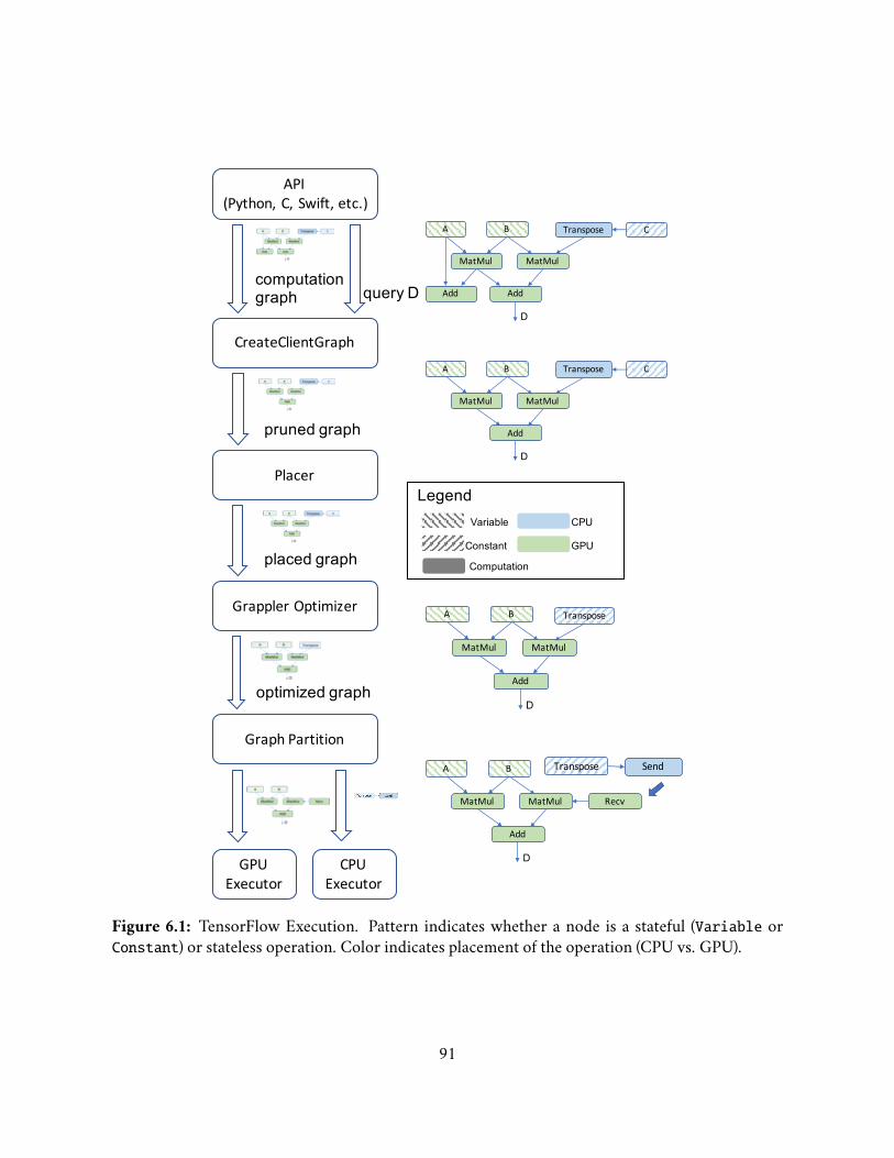
API (Python, C, Swift, etc.)

CreateClientGraph

query Dcomputation graph

pruned graph

Placer

placed graph

Grappler Optimizer

optimized graph

Graph Partition

GPU Executor

CPU Executor

A B C

MatMul MatMul

Add Add

D

Transpose

A B C

MatMul MatMul

Add

D

Transpose

D

A B

MatMul MatMul

Add

Transpose

Variable

Constant

Computation

CPU

GPU

A B

MatMul MatMul

Add

D

Recv

Transpose Send

Legend

Figure 6.1: TensorFlow Execution. Pattern indicates whether a node is a stateful (Variable orConstant) or stateless operation. Color indicates placement of the operation (CPU vs. GPU).

91

Programming Model. A TensorFlow application defines a computation, such as the for-ward pass of a neural network, as a directed graph, whose nodes represent operations. Edgesbetween nodes represent output tensors that are fed into successor operations. While mostoperations (such as MatMul and Conv2D) are stateless functions, TensorFlow introduces aVariable operation to represent frequently updated model parameters. A Variable holdsan internal buffer and outputs a reference handle to the buffer when executed. The refer-ence handle allows other operations to read and update the Variable’s value in place. Tosimplify the implementation of SGD algorithm, TensorFlow supports automatic differenti-ation that generates back-propagation computation from the user-defined forward compu-tation. TensorFlow also supports an application program explicitly declaring a placementconstraint for each operation and thus allows a single computation graph to utilize a het-erogeneous set of computing devices.Graph Execution. After defining the computation graph, a TensorFlow application pro-gram may query an operation’s output, e.g., D in Fig. 6.1, which triggers graph execution.The requested value might depend on only a subset of operations in the computation graphand thus TensorFlow first creates an execution graph by pruning unnecessary operations.TensorFlow places operations of this execution graph onto computing devices, includingGPUs, CPUs and TPUs, subject to the placement constraints specified by the applicationprogram. After placement, the execution graph is run through a series of optimizationpasses in Grappler, such as memory optimization, and constant folding. To facilitate com-putation across a set of distributed devices, TensorFlow adds a pair of Send and Receiveoperations that transmit tensors across devices. TensorFlow partitions the execution graphamong a set of executors, each corresponding to a compute device.

An executor’s subgraph is executed in a breadth-first fashion, which begins with one ofthe executors executing a global SOURCE node which has no input dependency. When anexecutor finishes executing a node, it schedules to a thread pool all of its successors whosedependencies have been satisfied. A node’s successor could be a Send node that sends acontrol signal which triggers the execution of another executor’s subgraph. Note that whena node has a large fanout, the order in which its successor nodes are executed depends onthe runtime schedule and can vary greatly, leading to challenges when aiming to limit theirpeak total memory usage.MemoryManagement. TensorFlow allocatesVariable (model parameters) andConstantnodes as persistent tensors, which holds memory until graph destruction. Unlike MXNet [34]and SuperNeurons [153], TensorFlow dynamically allocates memory for operations’ out-puts during graph execution. When an operation generates an output tensor, a referencehandle to the tensor is assigned to each successor operation that consumes the tensor. Andthe tensor’s reference count is incremented for each successor operation. After an opera-tion is executed, TensorFlow decrements the reference count of its input tensors and freesa tensor when its reference count reaches zero. Dynamic memory allocation allows Ten-sorFlow to reuse device memory for other operations. Like computation execution order,memory consumption during training depends on computation scheduling and is highly

92

variable.GraphOptimization. TensorFlow’s Grappler module encompasses a number of optimiza-tion passes to improve execution speed and memory footprint of the computation graph.There are two Grappler optimizations that could considerably affect memory consump-tion and we briefly discuss them here. When a GPU’s peak memory consumption exceedsthe GPU’s memory capacity during simulation, the Grappler memory optimizer performsa swapping pass that adds SwapOut and SwapIn nodes to offload GPU tensors to host mem-ory and prefetch them to GPU before they are needed. This swapping pass makes the besteffort to reduce peak memory consumption with minimal runtime overhead. However, inour experiments, we found that the swapping pass provides no benefit for scaling ResNet’sdepth or MoE’s number of experts (for both single-GPU and distributed settings). Ten-sorFlowMem also performs memory swapping, but possibly on different tensors and atdifferent times, which may lead to conflicting swapping decisions. To avoid the complica-tion of dealing with potential comflicts, TensorFlowMem supersedes Grappler’s swappingpass and we compare with TensorFlow with Grappler’s swapping pass disabled. Grappleralso performs a constant folding optimization that folds a subgraph into a single Constantnode that holds the result of the subgraph when the subgraph always evaluates to a constant.Constant folding reduces redundant computation but incurs higher memory consumptionto store the previously evaluated result. In next section, we discuss TensorFlowMem’s mem-ory optimizations.

6.3 Memory Optimizations for TensorFlow

In this section, we present memory optimizations for TensorFlow to reduce GPU memoryconsumption during training.

6.3.1 AMotivating Example

Expert 1 Expert 2 Expert n….

Previous layer

Gating

Figure 6.2: Mixture of Experts layer: example non-linear architecture.

93

As mentioned before, the key idea of TensorFlowMem is partitioned execution and swap-ping intermediate results between GPU and CPU memory. Generally speaking, how a graphis partitioned is key to performance. When the graph is composed of a sequence of complexlayers, it might be suitable to partition the computation graph layer by layer, which is theapproach taken by GeePS [46] and vDNN [128]. However, in a general dataflow graph, itis difficult to apply this approach to a fine-grained graph, where the number of operationsis much larger than the number of logical layers and operations are not associated with thelogical layer information.

Even when such layer-wise grouping can be achieved or approximated, for example, byassigning operations of the same depth to the same graph partition, a single partition mayproduce too many intermediate results within the partition and exhaust the limited mem-ory of the GPU devices or locate results across partitions incuring high communicationoverhead when accessed.

An example of such large complex layer is the Mixture of Experts (MoE) layer [135], asdepicted in Fig. 6.2. As a layer in a neural network, a single MoE may contain up to hundredsof thousands of smaller networks, referred to as experts. Each expert typically contains a fewmillion parameters. The output from the previous layer sparsely activates some of the ex-perts depending on the output of a gating network. An MoE layer has two distinguishingfeatures. Firstly, an MoE layer has a large number of branches, i.e. experts running in par-allel, resulting in a non-linear graph topology. Secondly, a single MoE layer may contain upto hundreds of billions of parameters. While a breath-first scheduling strategy as used inTensorFlow maximizes parallelism by executing as many branches in parallel as possible, itmay require a massive amount of memory. Therefore, we desire a graph partitioning strat-egy that applies to non-linear graphs consisting of the finer-grained operations within eachindividual layer.

Fig. 6.4a plots the memory consumption during a single mini-batch of training a Trans-former w/ MoE model, which uses MoE as its feed-forward layer instead of the originaldense-relu-dense layer. In this example, this model contains 12 MoE layers in total, with 32experts per MoE layer and 2 million parameters per expert, resulting in a model with over800 million parameters. TensorFlow reaches its peak memory at the end of the forwardpropagation, at around 400ms.

6.3.2 Partitioned Execution andMemory Swapping

Finding a graph execution schedule that minimizes memory consumption is an NP-completeproblem [107]. One heuristic to constrain the memory consumption of a non-linear graphis to topologically sort the graph nodes and execute them sequentially in the topologicallysorted order. However, sequentially executing all nodes restricts parallelism. We desire asolution that executes some operations in parallel to exploit available compute power whileachieving bounded memory usage. Instead, we propose to run partitions of the graph ratherthan single nodes sequentially, which exploits parallelism within a partition with a boundednumber of nodes. For example, as shown in Fig. 6.3, we may partition the MoE layer into 2

94

Expert 1 Expert 2 Expert n…

Previous layer

Gating

Expert 3 Expert 4

Figure 6.3: Partition the computation graph to constrain memory consumption. Node color de-notes expert partition.

experts per partition.Partitioned Execution. Based on these insights, we present a best-effort algorithm (Alg. 4)that partitions the computation graph of each device. The partitioned computation graphexecutes at most two partitions at a tiem while maximizing parallelism within each indi-vidual partition. Alg. 4 is applied to the optimized execution graph in TensorFlow beforeSend and Recv operations are added. Alg. 4 essentially performs a depth-first traversal ofeach device’s computation graph and assigns nodes to fixed-size partitions according to thetraversal order. Depth-first traversal makes best effort to consume intermediate results assoon as they are produced, instead of holding them in memory for longer durations.

A graph partition may generate intermediate results that are consumed by partitionsthat are many sequential steps away in the computation schedule. TensorFlowMem tem-porarily offloads the intermediate result tensors to host memory and prefetches them byadding SwapOut and SwapIn nodes. Because TensorFlowMem executes graph partitions ina pre-determined order, intermediate results that are not needed by the next K (by default,we use K = 2 in the following discussion and our experiments) partitions can be swappedout to host memory with low probability of interfering with computation. Similarly, Ten-sorFlowMem prefetches a tensor from host memory when it’s needed by partitions that willbe executed next. TensorFlowMem adds SwapOut and SwapIn nodes to proper partitionsbased on the execution order so offloading and prefetching are performed at the right time.Executor. TensorFlowMem revises TensorFlow’s operation scheduler to ensure at most 2partitions are executed at the same time. TensorFlowMem keeps track of the number of op-erations in each graph partition and the number of completed operations in each partition.The TensorFlowMem executor does not schedule any operation from partition t + 2 untilall operations from partition t have been completed. The ready-to-execute operations frompartition t+ 2 are buffered and scheduled as soon as partition t completes.

Fig. 6.4b depicts the memory consumption of TensorFlow with partitioned graph exe-cution and memory swapping using a partition size of 20 operations. We observe the peak

95

0 200 400 600 800 1000time (milliseconds)

0.00

0.25

0.50

0.75

1.00

num

ber o

f byt

es in

use 1e10

(a) Vanilla TensorFlow

0 500 1000 1500 2000 2500time (milliseconds)

0.00

0.25

0.50

0.75

1.00

num

ber o

f byt

es in

use 1e10

(b) + Partitioned execution & swapping

0 1000 2000 3000time (milliseconds)

0.00

0.25

0.50

0.75

1.00

num

ber o

f byt

es in

use 1e10

(c) + Placement

Figure 6.4: Understanding TensorFlow Memory Consumption: Transformer w/ MoE

96

Algorithm 4: Partition the computation graphinput : graph, devices, partSizeoutput: graphperDevReadyStack← EmptyMap() ;perDevPartNum← EmptyMap() ;perDevPartSize← EmptyMap() ;whileNot all graph nodes are assigned to some partition do

forall device ∈ devices doif perDevReadyStack[device] is not empty thennode← perDevReadyStack[device].pop();node.partition = perDevPartNum[node.device];perDevicePartSize[node.device] += 1;if perDevPartSize[node.device] == partSize thenperDevPartSize[node.device] = 0;perDevPartNum[node.device] += 1;

forall suc ∈ node.successors dosuc.numReadyInputs += 1;if suc.numReadyInputs == suc.inputSize thenperDevReadyStack[suc.device].push(suc);

memory consumption is reduced to 6.8GB from 9.5GB. The reduced memory consumptiondoes come with a runtime overhead of 2.5× in terms of time per mini-batch, due to the re-duced parallelism and additional data communication between GPU and CPU. Intuitivelyreducing the partition size reduces memory consumption and increasing the partition sizeincreases parallelism. Tuning the partition size gives a different trade-off between memoryconsumption and computation throughput.

6.3.3 Operation Placement

A computation graph may contain Variable and Constant nodes that are stateful opera-tions. Those operations contain an internal buffer that is allocated as a persistent tensorand is not deallocated until graph destruction. Typically, Variables and Constants are de-fined by the application program. These nodes are typically packaged with computationoperations that use them as an integral building block by higher level programming inter-faces, such as Keras [40]. When the application program places the computation operationon GPUs, Variables and Constants are implicitly placed on GPUs as well due to limitedprogramming flexibility. Constant folding folds a subgraph into a Constant operation. Thegenerated Constant operation are placed on the same computing device as the computationoperations.Variable and Constant nodes may consume a considerable amount of memory espe-

cially when the neural network contains a large number of parameters. Based on this ob-

97

servation, TensorFlowMem places Variable and Constant nodes on CPU and loads theirvalue to GPU when needed.

Op1W1

Send Recv

BackOp1

Op2

…

BackOp2

…CPU GPU

(a) TensorFlow inserts one pair of Send and Recv operations for all opera-tions that use the same VariableW1.

Op1W1

Send Recv

BackOp1

Op2

…

BackOp2

…

CPU GPU

Send Recv

(b) TensorFlowMem inserts one pair of Send and Recv for each operationthat uses VariableW1.

Figure 6.5: Placement optimization.

Separate communication. As shown in Fig. 6.5a, TensorFlow inserts one pair of Sendand Recv operations for all operations that use the same Variable or Constant placed ona different device. The received tensor value is used by multiple operations, for example, inthe forward pass as well as the backward pass of the same operation. Moreover, since Senddepends only on the Variable to be sent, the Variables’ value are received at the beginningof a mini-batch computation, regardless of when they are used, and buffered until the lastusage is completed.

To reduce memory consumption, TensorFlowMem inserts distinct pairs of Send andRecv operations for different operations that use the same Variable or Constant. Ten-sorFlowMem assigns the inserted Send and Recv operations to the partition that is shortlybefore the partition that needs the Variable or Constant, so they are executed shortly be-fore the data value is needed without blocking the computation. As shown in Fig. 6.4c, theplacement optimization further reduces peak memory consumption to 3.3GB. The effec-tiveness of our techniques is also observed for neural networks that do not contain a MoElayer such as Transformer [149]. However, the benefit from operation placement is rela-tively small for models with small number of parameters.

98

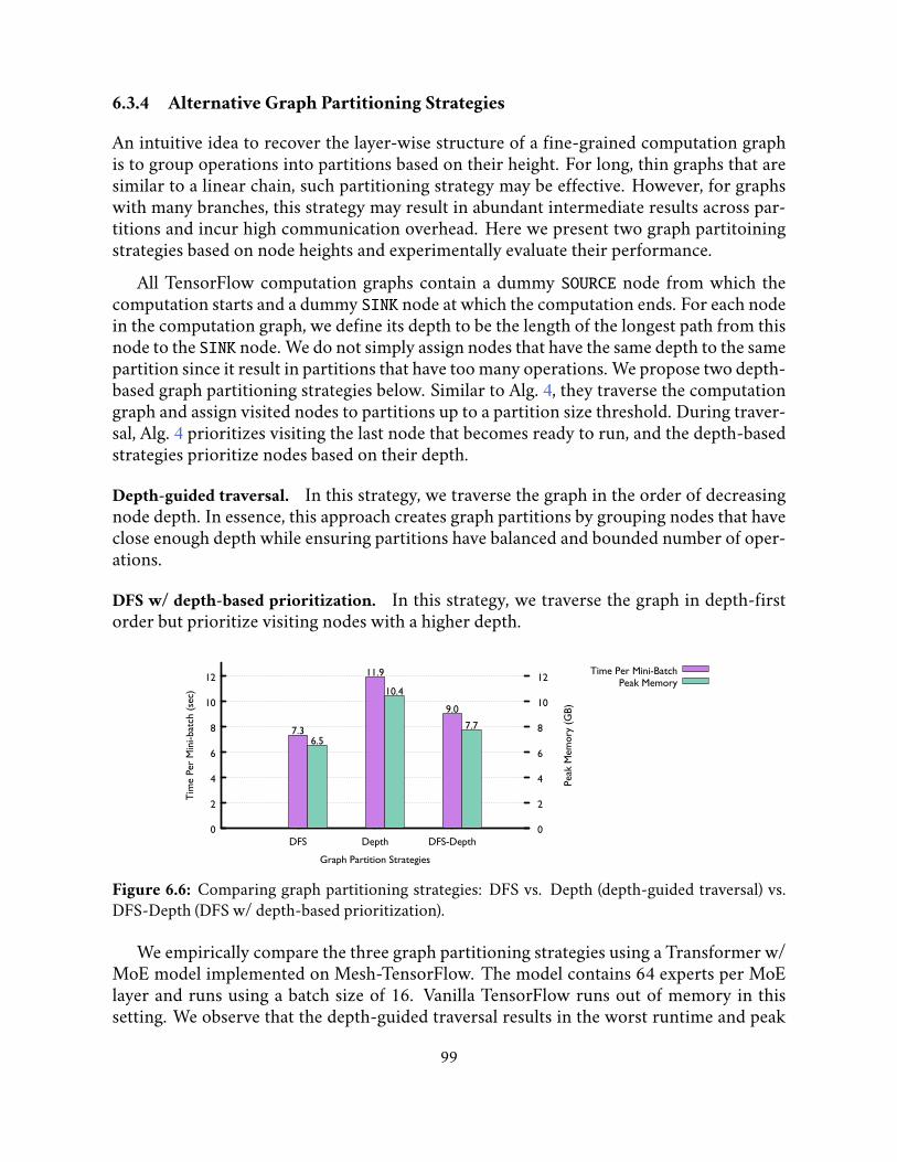
6.3.4 Alternative Graph Partitioning Strategies

An intuitive idea to recover the layer-wise structure of a fine-grained computation graphis to group operations into partitions based on their height. For long, thin graphs that aresimilar to a linear chain, such partitioning strategy may be effective. However, for graphswith many branches, this strategy may result in abundant intermediate results across par-titions and incur high communication overhead. Here we present two graph partitoiningstrategies based on node heights and experimentally evaluate their performance.

All TensorFlow computation graphs contain a dummy SOURCE node from which thecomputation starts and a dummy SINK node at which the computation ends. For each nodein the computation graph, we define its depth to be the length of the longest path from thisnode to the SINK node. We do not simply assign nodes that have the same depth to the samepartition since it result in partitions that have too many operations. We propose two depth-based graph partitioning strategies below. Similar to Alg. 4, they traverse the computationgraph and assign visited nodes to partitions up to a partition size threshold. During traver-sal, Alg. 4 prioritizes visiting the last node that becomes ready to run, and the depth-basedstrategies prioritize nodes based on their depth.

Depth-guided traversal. In this strategy, we traverse the graph in the order of decreasingnode depth. In essence, this approach creates graph partitions by grouping nodes that haveclose enough depth while ensuring partitions have balanced and bounded number of oper-ations.

DFS w/ depth-based prioritization. In this strategy, we traverse the graph in depth-firstorder but prioritize visiting nodes with a higher depth.

0

2

4

6

8

10

12

DFS Depth DFS-Depth 0

2

4

6

8

10

12

Time Per Mini-batch

(sec)

Peak

Memory (GB)

Graph Partition Strategies

Time Per Mini-Batch

7.3

11.9

9.0

Peak Memory

6.5

10.4

7.7

Figure 6.6: Comparing graph partitioning strategies: DFS vs. Depth (depth-guided traversal) vs.DFS-Depth (DFS w/ depth-based prioritization).

We empirically compare the three graph partitioning strategies using a Transformer w/MoE model implemented on Mesh-TensorFlow. The model contains 64 experts per MoElayer and runs using a batch size of 16. Vanilla TensorFlow runs out of memory in thissetting. We observe that the depth-guided traversal results in the worst runtime and peak

99

3.723.49

2.72.475.76E+09 5.83E+09

8.02E+09

9.76E+09

Graph Partition Size

seco

nds

byte

s

0

1

2

3

4

5

0.00E+00

2.50E+09

5.00E+09

7.50E+09

1.00E+10

1.25E+10

10 20 100 200

Time Per Mini-batch Peak Memory Usage

Tuning Graph Partition Size

Figure 6.7: The effect of graph partition size

memory consumption because the large amount of intra- and inter-partition intermediateresults. This result suggests that the computation graph is likely to contain a large numberof branches. DFS achieves better performance than DFS w/ depth-based prioritization,suggesting that prioritizing visiting the last node that becomes ready to run is more likelyto consume the intermediate results.

6.3.5 The Effect of Graph Partition Size

We run a Transformer model implemented on Mesh-TensorFlow to demonstrate the effectof graph partition size. As shown in Fig. 6.7, a larger partition size consumes more memorysince there are more operations in each partition. A larger partition also leads to a highexecution speed because there are fewer partitions and few inter-partition data movements.For any given problem, the optimal partition size depends on the available memory on theGPU device.

6.4 Evaluation

TensorFlowMem is implemented in TensorFlow v1.12.0 which we use as the baseline. Inthis section, we present a comprehensive experimental evaluation of TensorFlowMem. Allthe experiments are conducted in a private cluster, where each machine has a 16-core IntelXeon E5-2698B v3 processor with hyper-threading, 64GB of DRAM and a Titan X GPUwith 12GB device memory. The machines are interconnected with 40Gbps Ethernet.

100

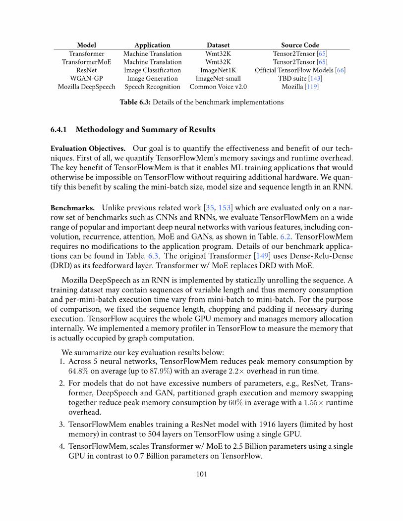
Model Application Dataset Source CodeTransformer Machine Translation Wmt32K Tensor2Tensor [65]

TransformerMoE Machine Translation Wmt32K Tensor2Tensor [65]ResNet Image Classification ImageNet1K Official TensorFlow Models [66]

WGAN-GP Image Generation ImageNet-small TBD suite [143]Mozilla DeepSpeech Speech Recognition Common Voice v2.0 Mozilla [119]

Table 6.3: Details of the benchmark implementations

6.4.1 Methodology and Summary of Results

Evaluation Objectives. Our goal is to quantify the effectiveness and benefit of our tech-niques. First of all, we quantify TensorFlowMem’s memory savings and runtime overhead.The key benefit of TensorFlowMem is that it enables ML training applications that wouldotherwise be impossible on TensorFlow without requiring additional hardware. We quan-tify this benefit by scaling the mini-batch size, model size and sequence length in an RNN.

Benchmarks. Unlike previous related work [35, 153] which are evaluated only on a nar-row set of benchmarks such as CNNs and RNNs, we evaluate TensorFlowMem on a widerange of popular and important deep neural networks with various features, including con-volution, recurrence, attention, MoE and GANs, as shown in Table. 6.2. TensorFlowMemrequires no modifications to the application program. Details of our benchmark applica-tions can be found in Table. 6.3. The original Transformer [149] uses Dense-Relu-Dense(DRD) as its feedforward layer. Transformer w/ MoE replaces DRD with MoE.

Mozilla DeepSpeech as an RNN is implemented by statically unrolling the sequence. Atraining dataset may contain sequences of variable length and thus memory consumptionand per-mini-batch execution time vary from mini-batch to mini-batch. For the purposeof comparison, we fixed the sequence length, chopping and padding if necessary duringexecution. TensorFlow acquires the whole GPU memory and manages memory allocationinternally. We implemented a memory profiler in TensorFlow to measure the memory thatis actually occupied by graph computation.

We summarize our key evaluation results below:1. Across 5 neural networks, TensorFlowMem reduces peak memory consumption by

64.8% on average (up to 87.9%) with an average 2.2× overhead in run time.2. For models that do not have excessive numbers of parameters, e.g., ResNet, Trans-

former, DeepSpeech and GAN, partitioned graph execution and memory swappingtogether reduce peak memory consumption by 60% in average with a 1.55× runtimeoverhead.

3. TensorFlowMem enables training a ResNet model with 1916 layers (limited by hostmemory) in contrast to 504 layers on TensorFlow using a single GPU.

4. TensorFlowMem, scales Transformer w/ MoE to 2.5 Billion parameters using a singleGPU in contrast to 0.7 Billion parameters on TensorFlow.

101

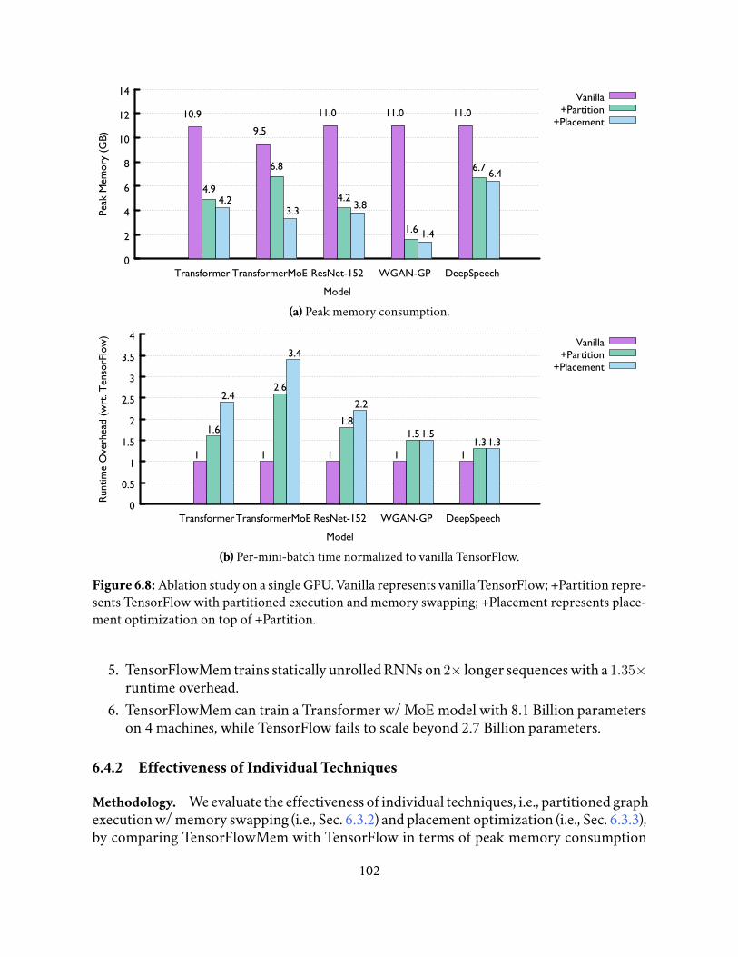
0

2

4

6

8

10

12

14

Transformer TransformerMoE ResNet-152 WGAN-GP DeepSpeech

Peak

Memory (GB)

Model

Vanilla

10.9

9.5

11.0 11.0 11.0 +Partition

4.9

6.8

4.2

1.6

6.7

+Placement

4.23.3 3.8

1.4

6.4

(a) Peak memory consumption.

0

0.5

1

1.5

2

2.5

3

3.5

4

TransformerTransformerMoE ResNet-152 WGAN-GP DeepSpeech

Runtime Overhead (wrt. TensorFlow)

Model

Vanilla

1 1 1 1 1

+Partition

1.6

2.6

1.81.5

1.3

+Placement

2.4

3.4

2.2

1.51.3

(b) Per-mini-batch time normalized to vanilla TensorFlow.

Figure 6.8: Ablation study on a single GPU. Vanilla represents vanilla TensorFlow; +Partition repre-sents TensorFlow with partitioned execution and memory swapping; +Placement represents place-ment optimization on top of +Partition.

5. TensorFlowMem trains statically unrolled RNNs on 2× longer sequences with a 1.35×runtime overhead.

6. TensorFlowMem can train a Transformer w/ MoE model with 8.1 Billion parameterson 4 machines, while TensorFlow fails to scale beyond 2.7 Billion parameters.

6.4.2 Effectiveness of Individual Techniques

Methodology. We evaluate the effectiveness of individual techniques, i.e., partitioned graphexecution w/ memory swapping (i.e., Sec. 6.3.2) and placement optimization (i.e., Sec. 6.3.3),by comparing TensorFlowMem with TensorFlow in terms of peak memory consumption

102

and time per mini-batch. We conduct this ablation study on Transformer (with both DRDand MoE versions), ResNet-152, WGAN-GP and DeepSpeech on a single Titan X GPU. ForDeepSpeech, the sequence length is fixed to 165. All models are trained with a partition sizeof 20 except for DeepSpeech, which uses a partition size of 5. A smaller partition size (5 vs.20) allows TensorFlowMem to more aggressively reduce memory consumption with a rel-atively small overhead for DeepSpeech. All models are executed using the largest possiblemini-batch that TensorFlow can support on a 12GB GPU.

Fig. 6.8a shows the peak memory consumption and Fig. 6.8b shows the time per mini-batch normalized to the baseline (i.e., vanilla TensorFlow). We compute the average peakmemory and average per-mini-batch time across all models, i.e., Avg, and across all modelsexcept for Transformer w/ MoE, i.e., Avg-NoMoE. We separate Transformer w/ MoE fromother models because MoE contains a distinctively large number of parameters comparedto other models.

Vanilla +Partition +Placement

Memory Consumption Average 10.8 4.8 3.8Average w/o MoE 11.0 4.4 4.0

Runtime Overhead Average 1 1.8 2.2Average w/o MoE 1 1.55 1.85

Table 6.4: Average memory consumption and runtime overhead across all models.

GPUMemory reduction. From Fig. 6.8a, we observe that TensorFlowMem reduces GPUmemory consumption by 65% on average across all models and by 87% for WGAN-GP.While the placement optimization further reduces memory consumption by 36.8% on topof partitioned execution and memory swapping for Transformer w/ MoE, it only brings asmall benefit to the other models that have relatively small number of parameters.

Runtimeoverhead. Fig. 6.8b shows that TensorFlowMem incurs a 2.2× slowdown in termsof time per mini-batch in average. The runtime overhead vary greatly across models. It canbe as large as 3.4× for Transformer w/ MoE and as small as 30% for DeepSpeech. Note thatfor models without a huge number of parameters, we achieve a 65% memory reduction witha 55% runtime overhead using only partitioned graph execution and memory swapping.

Model TensorFlow TensorFlowMemTransformer 11264 (words) 25600 (words)

Transformer w/ MoE 4 (sentence pairs) 40 (sentence pairs)ResNet-152 57 (images) 186 (images)WGAN-GP 90 (images) 324 (images)

Table 6.5: The maximum supported mini-batch size by both systems

103

Model TensorFlow TensorFlowMemTransformer 8731 (words / sec) 3699 (words / sec)

Transformer w/ MoE 4.6 (s. pairs /sec) 5.2 (s. pairs / sec)ResNet-152 50 (images / sec) 27 (images / sec)WGAN-GP 7.9 (images / sec) 4.5 (images / sec)

Table 6.6: Throughput using the maximum supported mini-batch size.

6.4.3 Training w/ Larger Mini-Batches

By reducing GPU memory consumption, TensorFlowMem allows applications to train mod-els using larger batch sizes. While the common wisdom for using larger batch size is toimprove computation throughput. There are cases where larger mini-batch sizes lead tohigher model accuracy, for example, as shown in GPipe [80]. TensorFlowMem providesusers an additional degree of freedom for using larger mini-batch sizes. Table. 6.5 showsthe largest mini-batch supported by TensorFlow and TensorFlowMem and Table. 6.6 showsthe computation throughput using the maximum batch size. For Transformer, ResNet andWGAN-GP, we observe that TensorFlowMem enables training 2.2−3.6× larger mini-batchsize with a 43% − 58% slowdown in computation throughput. TensorFlowMem supportsa 10× larger mini-batch size for Transformer w/ MoE, which contains an order of magni-tude more parameters than other models. TensorFlowMem also improves the computationthroughput for Transformer w/ MoE by 6%. TensorFlowMem enables a larger range of pos-sible mini-batch sizes compared to TensorFlow, allowing applications to tune mini-batchsize for high model quality, especially for models with a large number of parameters.

6.4.4 Training Larger Models

It has been shown that larger models achieve better accuracy across different applicationdomains [72, 73, 135]. The key benefit of TensorFlowMem is that it enables training largermodels that is otherwise impossible without using additional hardware. In this section,we demonstrate that TensorFlowMem enables training ResNet with 3.8×more layers andTransformer w/ MoE with 4.4×more parameters.

Deeper ResNet. Similar to previous work [35, 153], we increase the model capacity ofResNet by scaling its number of layers. Specifically, we follow SuperNeuron [153] and in-crease the number of the third block. Our result is present in Table 6.7. Using the samemini-batch size of 16 images, TensorFlowMem scales to 1916 layers while TensorFlowscales to only 504 layers. Using a mini-batch size of 32, TensorFlowMem scales to 1001layers. Moreover, TensorFlowMem fails to scale to deeper ResNet because of running outof host memory.

Mixture of Experts. We evaluate TensorFlowMem using Transformer w/MoE. Table 6.8shows the maximum number of experts per MoE layer which can trained using TensorFlowand TensorFlowMem. TensorFlowMem is able to train 48 experts for MoE layer, which is

104

4× as many as vanilla TensorFlow2.

System Mini-batch size #Layers #Param. ThroughputTensorFlow 16 504 172 Million 11.43

TensorFlowMem 16 1916 697 Million 1.76TensorFlowMem 32 1001 385 Million 4.04

Table 6.7: Maximum ResNet model size that can be trained on a single Titan X GPU and computa-tion throughput with different mini-batch size.

System #Experts #Param. ThroughputTensorFlow 12 / MoE 0.66 Billion 7.8 pairs / sec

TensorFlowMem 48 / MoE 2.5 Billion 1.2 pairs / sec

Table 6.8: Maximum number of experts that can be trained on a single TitanX GPU. We use a batchsize of 8 and graph partition size of 200.

Sequence Length 100 200 400 500 800TensorFlow 1.15 2.3 4.64 OOM OOM

TensorFlowMem 1.56 3.03 6.03 - 12

Table 6.9: RNN training: time per mini-batch (seconds) for different input sequence length.

6.4.5 Longer Recurrence Sequences

For RNNs, the sequence length is often limited by GPU memory size. TensorFlowMem en-ables training RNNs on longer sequences with a small runtime overhead, which we demon-strate using Mozilla DeepSpeech, which is a statically unrolled RNN. Our experiments usea mini-batch size of 128 sentences and the partition size of TensorFlowMem is set to 5. Ta-ble 6.9 shows that TensorFlowMem can train DeepSpeech on sequences of length 800 whileTensorFlow fails beyond sequence length of 400. Similar to ResNet, TensorFlowMem failsto scale to longer sequences due to the limited host memory. On the same sequence length,TensorFlowMem shows a runtime overhead of roughly 35%.

6.4.6 Distributed Model-Parallel Training

Next, we show that TensorFlowMem’s memory optimization techniques can be directly ap-plied to the distributed model-parallel setting as well. By utilizing 4 GPU machines, evenlarger models with more experts can be trained. Table 6.10 highlights these results. For allexperiments, we split only the experts dimension of tensors across the 4 nodes, and repli-cate all other dimensions. In the distributed setting, the memory optimizations in Ten-sorFlowMem are simply applied independently on each node. TensorFlowMem is able totrain a model with 8.1 billion parameters, 3× as many as vanilla TensorFlow in the samedistributed setting.

2We ran TensorFlow both with and without the Grappler memory swapping pass, but obtained the same result bothtimes.

105

System #Experts Param. Size ThroughputTensorFlow 52 / MoE 2.7 Billion 8.5 pairs /sec

TensorFlowMem 160 / MoE 8.1 Billion 0.93 pairs /sec

Table 6.10: Maximum number of experts that can be trained on 4 nodes each with a single TitanXGPU. We use a batch size of 8 and graph partition size of 200.

6.4.7 Comparison with RelatedWork

In this section, we compare TensorFlowMem with the TensorFlow’s native Grappler Mem-ory Optimizer and SuperNeurons [153] on scaling model capacity.

Grappler Memory Optimizer. The Grappler Memory Optimizer statically estimates thegraph execution time and memory consumption and invokes a swapping pass when andonly when the estimated memory consumption of at least one GPU exceeds its memory ca-pacity. The static estimation results also provides the start and end times of each operationand the memory footprint of each tensor. The swapping pass relies on this information toswap tensors in and out arond the memory peak to avoid running out of memory. Accord-ing to operations’ start and end time, control dependencies are added to the swap operationsso that they are executed at appropriate times to avoid stalling computation.

Model Mini-batch Size Grappler Memory Optimizer TensorFlowMemResNet 16 images 504 layers 1916 layers

Transformer w/ MoE 8 sentense pairs 12 experts / MoE 48 experts / MoE

Table 6.11: Largest model configuration supported by Grappler Memory Optimizer and Tensor-FlowMem.

Model Model Configuration Predicated OOM Actual OOMResNet 1001 layers False True

Transformer w/ MoE 48 experts / MoE True TrueTransformer N/A True True

Table 6.12: Grappler memory optimizer: simulator prediction and effectiveness.

Table 6.11 shows the largest ResNet and MoE model that TensorFlow (with GrapplerMemory Optimizer enabled) can run. Surprisingly, we found the Grappler Memory Opti-mizer does not improve upon TensorFlow in terms of model capacity. In order to under-stand why Grappler Memory Optimizer fails we analyzed three large models that result inOOM when executing on TensorFlow with Grappler Memory Optimzier (Fig. 6.12). Staticestimation fails to predict the OOM error for the ResNet mode with 504 layers. Whilestatic estimation correctly predicts the OOM error and the Grappler Memory Optimizerindeed adds swap operations for the two Transformer-based models, training still runs outof memory on GPU. Note that all three models can execute with TensorFlowMem with-out running out of memory. We speculate that the Grappler Memory Optimizer’s failureis due to the discrepency between static estimation and actual execution. Also, when the

106

OOM is due to a large fanout, it cannot be mitigated without intentionally delaying somecomputation.

SuperNeurons. SuperNeurons also relies on memory swapping to scale model capacitywith limited GPU memory. It effectively scales the mini-batch size for several convolu-tional neural networks and enables training much deeper ResNet [153]. However, it is aprototype implementation that does not support TensorFlow API. We compare our resultswith SuperNeurons’ as report by Wang et al. [153]. Using a single GPU with 12 GB of mem-ory, SuperNeurons scales ResNet to 1920 layers while TensorFlowMem scales ResNet to1916 layers (on a different GPU that has the same memory size). When training on Im-ageNet, SuperNeurons scales ResNet-152 to a maximum batch size of 176 images whileTensorFlowMem scales the maximum batch size to 186 images. Note that SuperNeuronsalso incurs none trivial overhead at when the model’s memory footprint exceeds the GPUmemory capacity. For examples, the computation throughput drops by nearly 30% whenscaling ResNet-152 to a mini-batch size of 80 images. TensorFlowMem suffers a 46% over-head when scaling mini-batch size to 186 images. SuperNeurons was not evaluated on otherDNN models besides CNNs.

6.5 Memory-Efficient Application Implementation on TensorFlow

Implementation of the DNN model affects its memory consumption. In this section, wepresent two application implementation guidelines that can enable scaling to larger models,especially when using TensorFlowMem. We demonstrate the effectiveness of these guide-lines by modifying Mesh-TensorFlow which is a library on top of TensorFlow for model-parallel training and the MoE implemenation that’s based on Mesh-TensorFlow. Togetherwith TensorFlowMem, these changes enable training a 7.5× larger MoE model than theoriginal implementations using TensorFlow.

6.5.1 Application Implementation Guidelines

Partition a large operation into smaller operations. TensorFlowMem’s partitioned execu-tion and memory swapping take each operation as an atomic unit. They fail to overcome thedevice memory constraint when a single operation consumes or produces a tensor that oc-cupies too large an amount of memory. The application program can alleviate this problemby partitioning a big operation that produces a few big tensors into many small operationsthat produce many small tensors, permitting graph partitioning and memory swapping towork at a finer granularity. There exist many opportunities to parallelize larger operations.Tensors that are too small may lead to inefficient use of massively parallel processing units,e.g., GPUs. Therefore, it is critical to partition tensors to the proper size. While we relyon users to manually, we expect future work may improve upon manual partitioning usingautomated search.

Allocate tensors propotionally to input size. In some DNNs, the size of the input to someoperations is dynamically determined. While it is convenient and fast to allocate a tensor

107

of fixed size to hold the largest possible input, this approach can waste a large amount ofmemory. This is particularly wasteful when a large tensor is dynamically split into smallertensors of variable size, such as in MoE. In this case, the application either allocates themaximum possible size for each dynamially allocated tensor, which is the input size, ordrops some of the input values. In case of OOM, it is better for applications to suffer a smallthroughput penalty and allocate memory propotionally to input size, for example, by usingthe sparse gather operation.

6.5.2 Over-Partitioning Operations in Mesh-TensorFlow

Mesh-TensorFlow [136] is a framework for model-parallel training on top of TensorFlow. Itpartitions the large operations of a computation graph and place the them on different com-puting devices. However, the number of partitions a Mesh-TensorFlow tensor may have isupper-bounded by the number of physical computing devices. Thus it may still result in alarge operation that consumes a large fraction of GPU memory by itself. To address thisissue, we designed and implemented Virtual Mesh-TensorFlow (VMesh-TensorFlow), an ex-tension to Mesh-TensorFlow, which partitions a large operation bound to a specific deviceinto smaller operations. VMesh-TensorFlow works in conjunction with partitioned graphexecution and memory swapping to enable execution of models whose memory consump-tion exceeds the overall memory capacity of all of the devices in the mesh.

Background: Mesh-TensorFlow

Like TensorFlow, Mesh-TensorFlow requires applications to define a computation graph.Tensors in a Mesh-TensorFlow computation graph have named dimensions and differenttensors may share the same name along some of their dimensions. Mesh-TensorFlow addi-tionally requires the application program to define a mesh shape and a mesh layout A meshshape defines a multi-dimensional grid composed of computing devices (e.g., GPUs), anda mesh layout is a mapping from named tensor dimensions to mesh dimensions. A Mesh-TensorFlow is lowered to a TensorFlow graph by partitioning the Mesh-TensorFlow tensorsalong dimensions that are mapped to a mesh dimension and replicating the tensors alongother mesh dimensions. In this way, a large tensor may be split across multiple computingdevices as well as the operations that generate and produce the tensor.

Virtual Mesh-TensorFlow

Mesh Over-partitioning. In Mesh-TensorFlow, the number of nodes in the mesh layoutequals the number of physical devices. For example, a mesh with shape (3, 2) corresponds to6 physical devices logically arranged in a 3× 2 grid. VMesh-TensorFlow additionally intro-duces a device shape that specifies a virtual grid for each device (we refer to the mesh shape inMesh-TensorFlow as cluster shape for clarity). VMesh-TensorFlow requires the device shapeand the cluster shape to have the same number of dimensions. Besides partitioning tensorsaccording to the cluster shape, VMesh-TensorFlow further partitions the tensors allocatedfor each device according to the device shape using the same logic. In other words, VMesh-

108

GPU0 GPU1 GPU2

GPU3 GPU4 GPU5

Figure 6.9: VMesh-TensorFlow example. There are 6 physical devices arranged in a logical gridwith cluster shape (3, 2). Each device is further partitioned with a device shape of (2, 2). The overallmesh used for compiling the Mesh-TensorFlow graph has shape (6, 4).

TensorFlow partitions tensors according to a mesh shape that is the element-wise productof the cluster shape and device shape (Fig. 6.9). Over-partitioning the mesh enables largetensors and operations to be split into finer-grained partitions on each physical device, andswapped into device memory individually. In our implementation, the Mesh-TensorFlowgraph is simply compiled using the virtual mesh instead of the original physical mesh, withno changes required to the application code. Similar techniques for using over-partitioningto abstract away physical devices have been explored in prior work [17, 126].Graph De-duplication. Although mesh over-partitioning enables finer-grained splittingof tensors and operations, it by itself introduces significant memory and performance over-head. In Mesh-TensorFlow, if a tensor is not split across a mesh dimension, then it is repli-cated across it. However, if that mesh dimension is over-partitioned by a factor of N (ie.its device shape dimension has sizeN ), then the tensor (and all operations using the tensor)will be replicated N times on each physical device3.

To overcome this limitation, we implement a de-duplication pass which runs when theVMesh-TensorFlow graph is compiled to a TF graph. The de-duplication pass finds anytensors, variables, and operations which are replicated multiple times on a single device,and replaces their uses with references to a single “master” copy. The other unused copiesare then pruned out by TensorFlow before execution.

6.5.3 Memory Effcient MoE Implementation

The techniques presented thus far in this section are generic framework improvementswhich can apply to existing model code. On the other hand, the model creator may achieve

3We note that the duplication issue is specific to Mesh-TensorFlow, other model-parallel frameworks may not havethe same limitation.

109

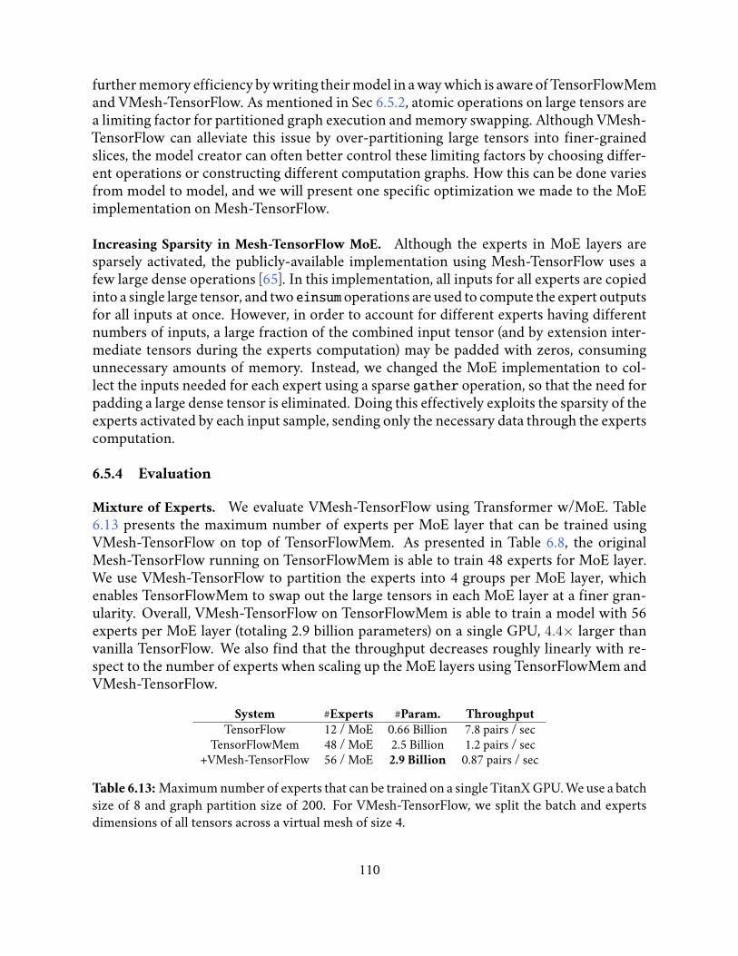
further memory efficiency by writing their model in a way which is aware of TensorFlowMemand VMesh-TensorFlow. As mentioned in Sec 6.5.2, atomic operations on large tensors area limiting factor for partitioned graph execution and memory swapping. Although VMesh-TensorFlow can alleviate this issue by over-partitioning large tensors into finer-grainedslices, the model creator can often better control these limiting factors by choosing differ-ent operations or constructing different computation graphs. How this can be done variesfrom model to model, and we will present one specific optimization we made to the MoEimplementation on Mesh-TensorFlow.

Increasing Sparsity in Mesh-TensorFlow MoE. Although the experts in MoE layers aresparsely activated, the publicly-available implementation using Mesh-TensorFlow uses afew large dense operations [65]. In this implementation, all inputs for all experts are copiedinto a single large tensor, and two einsum operations are used to compute the expert outputsfor all inputs at once. However, in order to account for different experts having differentnumbers of inputs, a large fraction of the combined input tensor (and by extension inter-mediate tensors during the experts computation) may be padded with zeros, consumingunnecessary amounts of memory. Instead, we changed the MoE implementation to col-lect the inputs needed for each expert using a sparse gather operation, so that the need forpadding a large dense tensor is eliminated. Doing this effectively exploits the sparsity of theexperts activated by each input sample, sending only the necessary data through the expertscomputation.

6.5.4 Evaluation

Mixture of Experts. We evaluate VMesh-TensorFlow using Transformer w/MoE. Table6.13 presents the maximum number of experts per MoE layer that can be trained usingVMesh-TensorFlow on top of TensorFlowMem. As presented in Table 6.8, the originalMesh-TensorFlow running on TensorFlowMem is able to train 48 experts for MoE layer.We use VMesh-TensorFlow to partition the experts into 4 groups per MoE layer, whichenables TensorFlowMem to swap out the large tensors in each MoE layer at a finer gran-ularity. Overall, VMesh-TensorFlow on TensorFlowMem is able to train a model with 56experts per MoE layer (totaling 2.9 billion parameters) on a single GPU, 4.4× larger thanvanilla TensorFlow. We also find that the throughput decreases roughly linearly with re-spect to the number of experts when scaling up the MoE layers using TensorFlowMem andVMesh-TensorFlow.

System #Experts #Param. ThroughputTensorFlow 12 / MoE 0.66 Billion 7.8 pairs / sec

TensorFlowMem 48 / MoE 2.5 Billion 1.2 pairs / sec+VMesh-TensorFlow 56 / MoE 2.9 Billion 0.87 pairs / sec

Table 6.13: Maximum number of experts that can be trained on a single TitanX GPU. We use a batchsize of 8 and graph partition size of 200. For VMesh-TensorFlow, we split the batch and expertsdimensions of all tensors across a virtual mesh of size 4.

110

Distributed Model-Parallel Training

System #Experts Param. Size ThroughputTensorFlow 52 / MoE 2.7 Billion 8.5 pairs /sec

TensorFlowMem 160 / MoE 8.1 Billion 0.93 pairs /sec+VMesh-TensorFlow 200 / MoE 10.1 Billion 0.52 pairs /sec

+SparseMoE 400 / MoE 20.2 Billion 1.6 pairs /sec

Table 6.14: Maximum number of experts that can be trained on 4 nodes each with a single TitanXGPU. We use a batch size of 8 and graph partition size of 200. For VMesh-TensorFlow and Sparse-MoE, we split the experts dimension of all tensors across a virtual mesh of size 20 (cluster shape of4 and device shape of 5).

Application-level optimizations in VMesh-TensorFlow and SparseMoE enable traininglarger models on TensorFlowMem using distributed model parallelism. We demonstrate itusing the same settings as used in Sec. 6.4.6 (totally 4 GPU machines), and the results arepresented in Table 6.10. As before, we split only the experts dimension of tensors across the4 machines and replicate all other dimensions.

TensorFlowMem+VMesh-TensorFlow. With VMesh-TensorFlow, we over-partition the meshby a factor of 5, resulting in a virtual mesh of size 20. This means that any tensors with anexperts dimension are split into 20 slices, 5 on each node. Combining TensorFlowMemwith VMesh-TensorFlow enables the number of experts per MoE layer to be increased to200, forming a model with over 10 billion parameters.

TensorFlowMem+VMesh-TensorFlow+SparseMoE. Lastly, we evaluate the sparse MoE im-plementation described in Sec 6.5.3. By combining TensorFlowMem, VMesh-TensorFlow,and SparseMoE, we are able to train 400 experts per layer, in a model which has over 20billion parameters. We also note that the throughput of training increased even when com-pared with training smaller models without SparseMoE. This is likely due to eliminatingredundant computations on padding values in large dense tensors. Similar to ResNet andTransformer w/ MoE on a single machine, we also observe that with larger MoE layers, thehost memory rather than GPU memory is exceeded, indicating that even larger models canbe trained with an expansion to host memory.

6.6 Summary

In this chapter, we present TensorFlowMem that reduce TensorFlow’s GPU memory con-sumption to enable training substantially larger models in both single GPU and distributedsettings. The distributed model-parallel application can be improved to better leverage Ten-sorFlowMem to train even larger models on the same hardware. TensorFlowMem demon-strates that scheduling where and when memory is allocated allows scaling model size witha small overhead. We expect that TensorFlowMem memory optimizations can be improvedby leveraging more accurate estimations of the operation execution time and memory foot-print.

111

Chapter 7

Conclusion and Future Directions

7.1 Conclusion

In this thesis, we demonstrate that the domain-specific characteristics of machine learningtraining can be leveraged to schedule hardware resources to improve the training speed andtrain larger models. Specifically, we present a mechanism for scheduling network commu-nication that improves the training convergence speed by up to 5×, a computation schedul-ing mechanism that further improves training speed, while consuming lower network band-width and substantially reducing programmer effort, and a memory scheduling mechanismthat enables training up to 7.5× larger models on the same hardware with acceptable per-formance overhead.

The ideas that we explore, such as value-based prioritization, scheduling computationto avoid conflicting accesses, and scheduling memory allocation based on computation, aregeneralizable to broad machine learning applications. However, their implementations andeffectiveness depend on the specific machine learning model, algorithm, as well as hardwarearchitecture. Machine learning is a fast advancing field. New models and improvementsto learning algorithms are being invented at a high pace. The success of machine learningmotivates new software systems and hardware architectures to be developed to better servethis important workload, which in turn makes it easier to develop and experiment with newmachine learning models and algorithms.

With the fast advancements in machine learning techniques, software systems and hard-ware architectures, the research focus on machine learning systems is shifting from networkand storage I/O to computation. Existing works on computation optimization are focusedon the memory bandwidth bottleneck, improving cache hit rate, exposing opportunities forparallelization and reducing the overhead of interacting with hardware accelerators.

7.2 Future Directions

In this section we discuss some opportunities and challenges in improving upon the tech-niques we present, generalizing them to newer machine learning models and across hard-

112

ware architectures.

7.2.1 Maximizing Training Speed Subject ToMemory Constraints

There exist many techniques to reduce GPU memory consumption and thus enable traininglarger models and they all involve a trade-off between memory consumption and computa-tion throughput or accuracy. Ultimately, our goal is to maximize training speed subject thedevice memory constraints. This problem is hard and in this section we discuss our visionin tackling this problem.

Techniques Trade-Off Notable Prior WorkScheduling Degree of parallelism TensorFlowMem

Gradient checkpointing Recomputation [35, 146]Anti-constant folding Recomputation TensorFlowMem

Memory swapping Communication TensorFlowMem, SuperNeurons [153]Device placement Communication TensorFlowMem

Lossless computation Computation Gist [81]Quantization Accuracy [41, 42, 98, 114]

Table 7.1: Summary of memory optimization techniques and their trade-offs[81].

Maximizing training speed subject to device memory constraints is a particularly hardproblem for the following reasons:

• Extremely large search space. As shown in Table 7.1, there exist many techniquesto optimize the memory consumption of DNN training and many techniques involvetuning parameters. For example, TensorFlowMem’s partitioned execution introducesa performance-sensitive parameter, partition size. It may also be important to decidewhich constant subgraph should be folded depending on the size of the result and thecomputation complexity, and what tensors to place on which devices based on the sizeof the operation and the communication bandwidth.

• Interdepenence between optimization techniques. Since the memory optimiza-tion techniques often affect each other, the order in which the optimizations are ap-plied is important. The interdependence between operations makes the search spaceexponentially hard.

• Hardware- andworkload-specific. The above mentioned techniques involve trade-off between memory consumption and different hardware resources or computationquality. The best configuration of techniques thus depend on the hardware and theDNN model. For example, in case there is abundant bandwidth between host and GPUmemory, aggressively placing large tensors on host memory would be more effectivethan introducing redundant computation.

• Memory efficientDAG scheduling is hard. It is an NP-complete problem to sched-ule a DAG to execute using minimal memory.

• Accurate simulation is difficult. Many the above techniques rely on knowing the

113

size of the tensors and operations’ execution time. While many of them simulate thegraph execution to obtain such information, accurate simulation is difficult as we’veshown in Sec. 6.4.7.

This problem is essentially a search problem over the space of memory optimziationtechniques.

7.2.2 Dynamic Scheduling for Dynamic Control Flow

In a dataflow system, application programs first construct a dataflow graph that describesthe computation, and then request the system to execute a subgraph or the whole graph.Although for many neural networks (e.g., AlexNet [95], Inception-v3 [144], and ResNet [72]),the computation can be described by a static acyclic directed graph (DAG) that applies toall data samples, there are many cases where the graph topology varies based on input orparameter values.Recurrent Neural Networks [55] model sequences of data (e.g., sentences). A recurrentneural network (RNN) repeatedly applies a cell function, such as long-short-term-memory(LSTM) [76], to each element of the sequence. Since sequences may have variable length,the cell function is executed for different number of times for different sequences. A typicalapproach for expressing RNNs as a static DAG is to statically unroll the sequence for a finitenumber of steps, padding shorter sequences with empty values and likely chopping longerones. An alternative approach is to construct a distinct graph for each input sequence, pay-ing the graph construction overhead for each data sample.RecursiveNeuralNetworks [141] generalize recurrent neural network to model arbitrarytopologies. For example, Tree-LSTM [145] models the syntactic tree of a sentence. Sincethe topology differs from sentence to sentence, Tree-LSTM constructs a distinct static DAGfor each sentence. As shown by Xu et al. [165], per-sample graph construction constitutes asignificant overhead (over 60% of runtime in some cases). Xu et al. [165] propose to resolvethe graph construction overhead by reusing the graph structure that already exists in thedataset instead of programmatic construction, restricting its applicability.Mixture of Experts (MoE) [135] is an example of conditional computation in neural net-works. A MoE layer consists of a gating network and a large number (up to hundreds ofthousands) of expert networks. Each data sample sparsely activates a small number of ex-perts as determined by the gating network based on runtime values. Therefore, for an inputmini-batch, the input size of each expert is unknown until the gating network has been ex-ecuted on the mini-batch.Expressing dynamic computation via dynamic control flow. Yu et al. [170] presenttwo dynamic control flow operations cond and while_loop in TensorFlow that representsconditional and iterateive computation respectively.

Recursive (including recurrent) neural networks can be expressed as a while loop iter-ating over the nodes in a topologically sorted order. As the loop body is represented as

114

a subgraph in a static DAG, all dynamic instances of the loop body (i.e., iterations) sharethe same dependency pattern. Therefore, for recursive neural networks, each iteration isconservatively specified to depend on its previous iteration to ensure correct ordering, re-sulting in a sequential execution, even though some iterations can potentially be executedin parallel. Jeong et al. [83] take advantage of the additional parallelism by introducing arecursion operation into TensorFlow. With recursion, a node recursively invokes the com-putation function on other nodes and waits until the recursive calls return to continue itsexecution. This allows a caller to dynamically specify its distinct dependency on the callees,permitting parallel execution of the functions on independent nodes.

The Need for Dynamic Scheduling of Dynamic Control Flow

Existing dataflow-based deep learning systems employ a static schedule derived prior tograph execution. This schedule determines how operations are placed on (possibly dis-tributed) computing devices and compiles each device’s graph partition to an executableprogram. As discussed earlier in Sec. 2.6, previous works propose to find an efficient sched-ule using machine learning when the same static computation graph applies to all data sam-ples. However, the effectiveness of this approach is limited when the computation graphdepends on input data and parameter values. In this section, we focus on distributed deviceplacement.Conditional Computation. TensorFlow’s cond is implemented using Switch which for-wards an input tensor to one of two subgraphs. MoE generalizes Switch in two ways: (1)the forwarding decision is made separately for each row in the input tensor and (2) each rowis forwarded toK out ofN subgraphs. Due to MoE’s large size (up to∼131 billion parame-ters), existing implementations (e.g., Tensor2Tensor [150] and Shazeer et al. [135]) staticallypartition the expert networks to different GPUs. Such static placement faces two problems:(1) the memory for a subgraph (e.g., variables) is statically allocated regardless of whethera subgraph is actually executed; (2) the input sizes among different experts can be highlyskewed. These issues lead to heavy over-provisioning of GPU memory while wasting GPUs’precious computing cycles. As reported by Shazeer et al. [135], a MoE layer consisting of131072 experts requires 128 Tesla K40 GPUs to fit while achieving a computation through-put of 0.3TFLOPS per GPU (Nvidia’s claimed peak throughput is 4.29TFLOPS/GPU). Withdynamic scheduling, the system allocates memory for only subgraphs that are executed andmay partition an overwhelmingly large input to an expert along with replicating the expertto multiple GPUs to balance load among GPUs.Iterative and Recursive Computation. TensorFlow creates a frame for each dynamic in-stance of the while_loop loop body. Operations of different frames may run in parallel aslong as their dependencies are satisfied. However, since each operation is statically placedonto one device, all frames of this operation is bound to this device. This can lead to sat-urating the computing power of a single device, thus missing the additional parallelism,such as observed by Jeong et al. [83]. Previous work on static device placement observesthroughput improvement when placing different iterations of a statically unrolled RNN to

115

different devices [86, 115, 116]. While static scheduling would be prohibitively expensivewhen different data samples require different graph topology, dynamic scheduling may dy-namically schedule different frames to different devices to take advantage of the additionalparallelism. Moreover, as recursion is restricted to trees, deep learning systems need a moregeneral approach for precisely capturing the dependency among loop iterations in order toexplore parallelism in arbitrary dependency topologies, such as Graph-LSTM [102].

116

Appendices

117

Appendix A

Orion Application Program Examples

A.1 Stochastic Gradient Descent Matrix Factorization

1 include("/path/to/orion/src/julia/orion.jl")

2 Orion.set_lib_path("/path/to/orion/lib/liborion_driver.so")

34 const master_ip = "10.117.1.17"

5 const master_port = 10000

6 const comm_buff_capacity = 1024

7 const num_executors = 64

8 const num_servers = 1

910 Orion.glog_init()

11 Orion.init(master_ip , master_port , comm_buff_capacity ,

12 num_executors , num_servers)

1314 const data_path = "file:///path/to/data.csv"

15 const K = 1000

16 const num_iterations = 256

17 const step_size = Float32(0.01)

1819 Orion.@accumulator err = 0

20 Orion.@accumulator line_cnt = 0

2122 Orion.@share function parse_line(line::AbstractString)

23 global line_cnt

24 line_cnt += 1

25 tokens = split(line, ',')

26 @assert length(tokens) == 3

27 key_tuple = (parse(Int64, String(tokens[1])),

28 parse(Int64, String(tokens[2])) )

29 value = parse(Float32, String(tokens[3]))

30 return (key_tuple , value)

31 end

118

3233 Orion.@share function map_init_param(value::Float32)::Float32

34 return value / 10

35 end

3637 Orion.@dist_array ratings = Orion.text_file(data_path , parse_line)

38 Orion.materialize(ratings)

39 dim_x, dim_y = size(ratings)

4041 println((dim_x, dim_y))

42 line_cnt = Orion.get_aggregated_value(:line_cnt, :+)

43 println("number of lines read = ", line_cnt)

4445 Orion.@dist_array W = Orion.randn(K, dim_x)

46 Orion.@dist_array W = Orion.map(W, map_init_param , map_values = true)

47 Orion.materialize(W)

4849 Orion.@dist_array H = Orion.randn(K, dim_y)

50 Orion.@dist_array H = Orion.map(H, map_init_param , map_values = true)

51 Orion.materialize(H)

5253 error_vec = Vector{Float64}()

54 time_vec = Vector{Float64}()

55 start_time = now()

5657 W_grad = zeros(K)

58 H_grad = zeros(K)

5960 @time for iteration = 1:num_iterations

61 Orion.@parallel_for for rating in ratings

62 x_idx = rating[1][1]

63 y_idx = rating[1][2]

64 rv = rating[2]

6566 W_row = @view W[:, x_idx]

67 H_row = @view H[:, y_idx]

68 pred = dot(W_row, H_row)

69 diff = rv - pred

70 W_grad .= -2 * diff .* H_row

71 H_grad .= -2 * diff .* W_row

72 W[:, x_idx] .= W_row .- step_size .* W_grad

73 H[:, y_idx] .= H_row .- step_size .* H_grad

74 end

75 @time if iteration % 4 == 1 ||

76 iteration == num_iterations

77 println("evaluate model")

78 Orion.@parallel_for for rating in ratings

79 x_idx = rating[1][1]

80 y_idx = rating[1][2]

81 rv = rating[2]

82 W_row = @view W[:, x_idx]

83 H_row = @view H[:, y_idx]

84 pred = dot(W_row, H_row)

85 err += (rv - pred) ˆ 2

86 end

119

87 err = Orion.get_aggregated_value(:err, :+)

88 curr_time = now()

89 elapsed = Int(Dates.value(curr_time - start_time)) / 1000

90 println("iteration = ", iteration , " elapsed = ", elapsed, " err = ", err)

91 Orion.reset_accumulator(:err)

92 push!(error_vec , err)

93 push!(time_vec , elapsed)

94 end

95 end

96 println(error_vec)

97 println(time_vec)

98 Orion.stop()

99 exit()

A.2 Sparse Logistic Regression

1 include("/path/to/orion/src/julia/orion.jl")

2 Orion.set_lib_path("/path/to/orion/lib/liborion_driver.so")

34 const master_ip = "127.0.0.1"

5 const master_port = 10000

6 const comm_buff_capacity = 1024

7 const num_executors = 16

8 const num_servers = 16

910 Orion.glog_init()

11 Orion.init(master_ip , master_port , comm_buff_capacity , num_executors ,

12 num_servers)

1314 const data_path = "file:///proj/BigLearning/jinlianw/data/kdda"

15 const num_iterations = 64

16 const step_size = Float32(0.00001)

17 const num_features = 20216830

1819 Orion.@accumulator err = Float32(0)

20 Orion.@accumulator loss = Float32(0)

21 Orion.@accumulator line_cnt = 0

2223 Orion.@share function parse_line(index::Int64, line::AbstractString)

24 global line_cnt += 1

25 tokens = split(strip(line), ' ')

26 label = parse(Int64, tokens[1])

27 if label == -1

28 label = 0

29 end

30 i = 1

31 feature_vec = Vector{Tuple{Int64, Float32}}(length(tokens) - 1)

32 for token in tokens[2:end]

33 feature = split(token, ":")

120

34 feature_id = parse(Int64, feature[1])

35 @assert feature_id >= 1

36 feature_val = parse(Float32, feature[2])

37 feature_vec[i] = (feature_id , feature_val)

38 i += 1

39 end

40 return ((index,), (label, feature_vec))

41 end

4243 Orion.@dist_array samples_mat = Orion.text_file(data_path ,

44 parse_line ,

45 is_dense = true,

46 with_line_number = true,

47 new_keys = true,

48 num_dims = 1)

49 Orion.materialize(samples_mat)

5051 line_cnt = Orion.get_aggregated_value(:line_cnt, :+)

52 println("number of lines read = ", line_cnt)

5354 Orion.@dist_array weights = Orion.rand(num_features)

55 Orion.materialize(weights)

5657 Orion.@share function sigmoid(z)

58 return Float32(1.0) ./ (Float32(1.0) .+ exp(-z))

59 end

6061 Orion.@share function safe_log(x)

62 if abs(x) < Float32(1e-15)

63 x = Float32(1e-15)

64 end

65 return log(x)

66 end

6768 Orion.@dist_array weights_buf = Orion.create_sparse_dist_array_buffer((weights.dims

...), Float32(0.0))

69 Orion.materialize(weights_buf)

7071 Orion.@share function apply_buffered_update(key, weight, update)

72 return weight + update

73 end

7475 Orion.set_write_buffer(weights_buf , weights, apply_buffered_update)

7677 error_vec = Vector{Float32}()

78 loss_vec = Vector{Float32}()

79 time_vec = Vector{Float64}()

80 start_time = now()

8182 for iteration = 1:num_iterations

83 Orion.@parallel_for for sample in samples_mat

84 sum = 0.0

85 label = sample[2][1]

86 features = sample[2][2]

87 for feature in features

121

88 fid = feature[1]

89 fval = feature[2]

90 sum += weights[fid] * fval

91 end

92 diff = sigmoid(sum) - label

93 for feature in features

94 fid = feature[1]

95 fval = feature[2]

96 weights_buf[fid] -= step_size * fval * diff

97 end

98 end

99 if iteration % 1 == 0 ||

100 iteration == num_iterations

101 Orion.@parallel_for for sample in samples_mat

102 sum = 0.0

103 label = sample[2][1]

104 features = sample[2][2]

105 for feature in features

106 fid = feature[1]

107 fval = feature[2]

108 sum += weights[fid] * fval

109 end

110111 if label == 1

112 loss += -safe_log(sigmoid(sum))

113 else

114 loss += -safe_log(1 - sigmoid(sum))

115 end

116 diff = sigmoid(sum) - label

117 err += abs2(diff)

118 end

119 err = Orion.get_aggregated_value(:err, :+)

120 loss = Orion.get_aggregated_value(:loss, :+)

121 curr_time = now()

122 elapsed = Int(Dates.value(curr_time - start_time)) / 1000

123 println("iteration = ", iteration , " elapsed = ", elapsed, " err = ", err, "

loss = ", loss)

124 push!(error_vec , err)

125 push!(loss_vec , loss)

126 push!(time_vec , elapsed)

127 Orion.reset_accumulator(:err)

128 Orion.reset_accumulator(:loss)

129 end

130 end

131132 println(error_vec)

133 println(loss_vec)

134 println(time_vec)

135 Orion.stop()

136 exit()

122

Bibliography

[1] Netflix Prize Data. https://www.kaggle.com/netflix-inc/netflix-prize-

data/. Last visited 2019-10-28. [Cited on page 78 and 78.][2] ClueWeb. https://lemurproject.org/clueweb12/. Last visited 2019-10-28.

[Cited on page 78.][3] ConvNet Burden. https://github.com/albanie/convnet-burden. Last visited

2019-10-28. [Cited on pages xiv and 18.][4] Apache Hadoop. https://hadoop.apache.org/. Last visited 2019-10-28. [Cited

on pages 1, 12, and 48.][5] Apache HBase. http://hbase.apache.org/. Last visited 2019-10-28. [Cited on

page 1.][6] Julia Micro-Benchmark. https://julialang.org/benchmarks/. Last visited Dec

2018. [Cited on page 62.][7] MATLAB Parallel For Loop. https://www.mathworks.com/help/matlab/ref/

parfor.html. Last visited Dec 2018. [Cited on page 63.][8] Apache Spark MLLib. https://spark.apache.org/mllib/. Last visited 2019-10-

28. [Cited on page 12.][9] Optimizing applications for numa. https://software.intel.com/en-us/

articles/optimizing-applications-for-numa. Last visited 2019-12-4. [Citedon page 8.]

[10] AI and Compute. https://openai.com/blog/ai-and-compute/. Last visited2019-10-28. [Cited on pages xiv, 17, and 18.]

[11] Tensorflow xla. https://github.com/plaidml/plaidml. Last visited 2019-11-9.[Cited on page 21.]

[12] rmsprop: Divide the gradient by a running average of its recent magni-tude. http://www.cs.toronto.edu/˜tijmen/csc321/slides/lecture_slides_lec6.pdf. Last visited 2019-12-8. [Cited on page 31.]

[13] Apache Spark. http://spark.apache.org/. Last visited 2019-10-28. [Cited onpages 1 and 48.]

[14] Tensorflow grappler memory optimizer. https://github.com/tensorflow/

tensorflow/tree/master/tensorflow/core/grappler/optimizers. Last visited

123

2019-10-28. [Cited on page 16.][15] Tensorflow xla. https://www.tensorflow.org/xla. Last visited 2019-11-9. [Cited

on page 21.][16] Martin Abadi, Paul Barham, Jianmin Chen, Zhifeng Chen, Andy Davis, Jeffrey Dean,

Matthieu Devin, Sanjay Ghemawat, Geoffrey Irving, Michael Isard, Manjunath Kud-lur, Josh Levenberg, Rajat Monga, Sherry Moore, Derek G. Murray, Benoit Steiner,Paul Tucker, Vijay Vasudevan, Pete Warden, Martin Wicke, Yuan Yu, and XiaoqiangZheng. Tensorflow: A system for large-scale machine learning. In 12th USENIXSymposium on Operating Systems Design and Implementation (OSDI 16), pages 265–283, 2016. URL https://www.usenix.org/system/files/conference/osdi16/osdi16-abadi.pdf. [Cited on pages 13, 22, 61, 75, 76, 76, 89, and 90.]

[17] Bilge Acun, Abhishek Gupta, Nikhil Jain, Akhil Langer, Harshitha Menon, EricMikida, Xiang Ni, Michael P. Robson, Yanhua Sun, Ehsan Totoni, LukaszWesolowski, and Laxmikant V. Kale. Parallel programming with migratable objects:Charm++ in practice. SC14: International Conference for High Performance Computing,Networking, Storage and Analysis, pages 647–658, 2014. [Cited on page 109.]

[18] A. Ahmed, M. Aly, J. Gonzalez, S. Narayanamurthy, and A. J. Smola. Scalable inferencein latent variable models. In WSDM ’12: Proceedings of the fifth ACM internationalconference on Web search and data mining, pages 123–132, New York, NY, USA, 2012.ACM. [Cited on page 12.]

[19] E.M. Airoldi, D.M. Blei, S.E. Fienberg, and E.P. Xing. Mixed membership stochasticblockmodels. J. Mach. Learn. Res., 9:1981–2014, 2008. [Cited on page 44.]

[20] Alham Fikri Aji and Kenneth Heafield. Sparse communication for distributed gra-dient descent. CoRR, abs/1704.05021, 2017. URL http://arxiv.org/abs/1704.05021. [Cited on page 15.]

[21] Rami Al-Rfou, Guillaume Alain, Amjad Almahairi, Christof Angermueller, DzmitryBahdanau, Nicolas Ballas, Frederic Bastien, Justin Bayer, Anatoly Belikov, Alexan-der Belopolsky, Yoshua Bengio, Arnaud Bergeron, James Bergstra, Valentin Bis-son, Josh Bleecher Snyder, Nicolas Bouchard, Nicolas Boulanger-Lewandowski,Xavier Bouthillier, Alexandre de Brebisson, Olivier Breuleux, Pierre-Luc Carrier,Kyunghyun Cho, Jan Chorowski, Paul Christiano, Tim Cooijmans, Marc-AlexandreCote, Myriam Cote, Aaron Courville, Yann N. Dauphin, Olivier Delalleau, JulienDemouth, Guillaume Desjardins, Sander Dieleman, Laurent Dinh, Melanie Ducoffe,Vincent Dumoulin, Samira Ebrahimi Kahou, Dumitru Erhan, Ziye Fan, Orhan Firat,Mathieu Germain, Xavier Glorot, Ian Goodfellow, Matt Graham, Caglar Gulcehre,Philippe Hamel, Iban Harlouchet, Jean-Philippe Heng, Balazs Hidasi, Sina Honari, Ar-jun Jain, Sebastien Jean, Kai Jia, Mikhail Korobov, Vivek Kulkarni, Alex Lamb, PascalLamblin, Eric Larsen, Cesar Laurent, Sean Lee, Simon Lefrancois, Simon Lemieux,Nicholas Leonard, Zhouhan Lin, Jesse A. Livezey, Cory Lorenz, Jeremiah Lowin,Qianli Ma, Pierre-Antoine Manzagol, Olivier Mastropietro, Robert T. McGibbon,Roland Memisevic, Bart van Merrienboer, Vincent Michalski, Mehdi Mirza, Al-

124

berto Orlandi, Christopher Pal, Razvan Pascanu, Mohammad Pezeshki, Colin Raffel,Daniel Renshaw, Matthew Rocklin, Adriana Romero, Markus Roth, Peter Sadowski,John Salvatier, Francois Savard, Jan Schluter, John Schulman, Gabriel Schwartz, Iu-lian Vlad Serban, Dmitriy Serdyuk, Samira Shabanian, Etienne Simon, Sigurd Spieck-ermann, S. Ramana Subramanyam, Jakub Sygnowski, Jeremie Tanguay, Gijs van Tul-der, Joseph Turian, Sebastian Urban, Pascal Vincent, Francesco Visin, Harm de Vries,David Warde-Farley, Dustin J. Webb, Matthew Willson, Kelvin Xu, Lijun Xue, Li Yao,Saizheng Zhang, and Ying Zhang. Theano: A Python framework for fast computa-tion of mathematical expressions. arXiv e-prints, abs/1605.02688, May 2016. URLhttp://arxiv.org/abs/1605.02688. [Cited on page 89.]

[22] Randy Allen and Ken Kennedy. Automatic translation of fortran programs to vectorform. ACM Transactions on Programming Languages and Systems, 9:491–542, 1987.[Cited on page 85.]

[23] Michael Armbrust, Reynold S. Xin, Cheng Lian, Yin Huai, Davies Liu, Joseph K.Bradley, Xiangrui Meng, Tomer Kaftan, Michael J. Franklin, Ali Ghodsi, and MateiZaharia. Spark sql: Relational data processing in spark. In Proceedings of the 2015ACM SIGMOD International Conference on Management of Data, SIGMOD ’15, pages1383–1394, New York, NY, USA, 2015. ACM. ISBN 978-1-4503-2758-9. doi: 10.1145/2723372.2742797. URL http://doi.acm.org/10.1145/2723372.2742797.[Cited on page 49.]

[24] Jeff Bezanson, Alan Edelman, Stefan Karpinski, and Viral B. Shah. Julia: A fresh ap-proach to numerical computing. SIAM Review, 59(1):65–98, 2017. doi: 10.1137/141000671. URL https://doi.org/10.1137/141000671. [Cited on pages 6 and 62.]

[25] Simone Bianco, Remi Cadene, Luigi Celona, and Paolo Napoletano. Benchmarkanalysis of representative deep neural network architectures. IEEE Access, 6:64270–64277, 10 2018. doi: 10.1109/ACCESS.2018.2877890. [Cited on pages xiv and 19.]

[26] David M. Blei, Andrew Y. Ng, and Michael I. Jordan. Latent dirichlet allocation. J.Mach. Learn. Res., 3:993–1022, March 2003. ISSN 1532-4435. URL http://dl.acm.org/citation.cfm?id=944919.944937. [Cited on pages 2, 44, 44, and 45.]

[27] Han Cai, Ligeng Zhu, and Song Han. Proxylessnas: Direct neural architecture searchon target task and hardware. CoRR, abs/1812.00332, 2018. URL http://arxiv.org/abs/1812.00332. [Cited on page 20.]

[28] Simone Campanoni, Glenn Holloway, Gu-Yeon Wei, and David Brooks. Helix-up:Relaxing program semantics to unleash parallelization. In Proceedings of the 13th An-nual IEEE/ACM International Symposium on Code Generation and Optimization, CGO’15, pages 235–245, Washington, DC, USA, 2015. IEEE Computer Society. ISBN 978-1-4799-8161-8. URL http://dl.acm.org/citation.cfm?id=2738600.2738630.[Cited on page 85.]

[29] Fay Chang, Jeffrey Dean, Sanjay Ghemawat, Wilson C. Hsieh, Deborah A. Wallach,Mike Burrows, Tushar Chandra, Andrew Fikes, and Robert E. Gruber. Bigtable: Adistributed storage system for structured data. ACM Trans. Comput. Syst., 26(2):4:1–

125

4:26, June 2008. ISSN 0734-2071. doi: 10.1145/1365815.1365816. URL http://doi.acm.org/10.1145/1365815.1365816. [Cited on page 1.]

[30] Mia Xu Chen, Benjamin N. Lee, Gagan Bansal, Yuan Cao, Shuyuan Zhang, Justin Lu,Jackie Tsay, Yinan Wang, Andrew M. Dai, Zhifeng Chen, Timothy Sohn, and YonghuiWu. Gmail smart compose: Real-time assisted writing. CoRR, abs/1906.00080, 2019.URL http://arxiv.org/abs/1906.00080. [Cited on page 2.]

[31] Rong Chen, Jiaxin Shi, Yanzhe Chen, and Haibo Chen. Powerlyra: Differentiatedgraph computation and partitioning on skewed graphs. In Proceedings of the TenthEuropean Conference on Computer Systems, EuroSys ’15, 2015. [Cited on pages 50, 75,77, 77, and 78.]

[32] Tianqi Chen and Carlos Guestrin. Xgboost: A scalable tree boosting system. In Pro-ceedings of the 22nd ACM SIGKDD International Conference on Knowledge Discovery andData Mining, KDD ’16, pages 785–794, New York, NY, USA, 2016. ACM. ISBN 978-1-4503-4232-2. doi: 10.1145/2939672.2939785. URL http://doi.acm.org/10.1145/2939672.2939785. [Cited on page 12.]

[33] Tianqi Chen, Mu Li, Yutian Li, Min Lin, Naiyan Wang, Minjie Wang, Tianjun Xiao,Bing Xu, Chiyuan Zhang, and Zheng Zhang. Mxnet: A flexible and efficient machinelearning library for heterogeneous distributed systems. ArXiv, abs/1512.01274, 2015.[Cited on page 13.]

[34] Tianqi Chen, Mu Li, Yutian Li, Min Lin, Naiyan Wang, Minjie Wang, Tianjun Xiao,Bing Xu, Chiyuan Zhang, and Zheng Zhang. Mxnet: A flexible and efficient ma-chine learning library for heterogeneous distributed systems. CoRR, abs/1512.01274,2015. URL http://dblp.uni-trier.de/db/journals/corr/corr1512.html#ChenLLLWWXXZZ15. [Cited on page 92.]

[35] Tianqi Chen, Bing Xu, Chiyuan Zhang, and Carlos Guestrin. Training deep nets withsublinear memory cost. ArXiv, abs/1604.06174, 2016. [Cited on pages 16, 101, 104,and 113.]

[36] Tianqi Chen, Thierry Moreau, Ziheng Jiang, Lianmin Zheng, Eddie Yan, HaichenShen, Meghan Cowan, Leyuan Wang, Yuwei Hu, Luis Ceze, Carlos Guestrin, andArvind Krishnamurthy. TVM: An automated end-to-end optimizing compiler fordeep learning. In 13th USENIX Symposium on Operating Systems Design and Im-plementation (OSDI 18), pages 578–594, Carlsbad, CA, 2018. USENIX Association.ISBN 978-1-931971-47-8. URL https://www.usenix.org/conference/osdi18/presentation/chen. [Cited on page 21.]

[37] Heng-Tze Cheng, Levent Koc, Jeremiah Harmsen, Tal Shaked, Tushar Chandra,Hrishi Aradhye, Glen Anderson, Greg Corrado, Wei Chai, Mustafa Ispir, Rohan Anil,Zakaria Haque, Lichan Hong, Vihan Jain, Xiaobing Liu, and Hemal Shah. Wide& deep learning for recommender systems. CoRR, abs/1606.07792, 2016. URLhttp://arxiv.org/abs/1606.07792. [Cited on page 2.]

[38] L. Chiariglione. Moving Picture Experts Group (MPEG). Scholarpedia, 4(2):6600,2009. doi: 10.4249/scholarpedia.6600. revision #91531. [Cited on page 15.]

126

[39] Trishul Chilimbi, Yutaka Suzue, Johnson Apacible, and Karthik Kalyanaraman.Project adam: Building an efficient and scalable deep learning training system. In 11thUSENIX Symposium on Operating Systems Design and Implementation (OSDI 14), pages571–582, Broomfield, CO, October 2014. USENIX Association. [Cited on page 13.]

[40] Francois Chollet. Keras. https://keras.io/, 2015. [Cited on page 97.][41] Matthieu Courbariaux and Yoshua Bengio. Binarynet: Training deep neural networks

with weights and activations constrained to +1 or -1. CoRR, abs/1602.02830, 2016.URL http://arxiv.org/abs/1602.02830. [Cited on pages 17 and 113.]

[42] Matthieu Courbariaux, Yoshua Bengio, and Jean-Pierre David. Training deep neuralnetworks with low precision multiplications, 2014. URL http://arxiv.org/abs/1412.7024. cite arxiv:1412.7024v5.pdfComment: 10 pages, 5 figures, Accepted as aworkshop contribution at ICLR 2015. [Cited on pages 17 and 113.]

[43] Paul Covington, Jay Adams, and Emre Sargin. Deep neural networks for youtuberecommendations. In Proceedings of the 10th ACM conference on recommender systems,pages 191–198. ACM, 2016. [Cited on page 2.]

[44] Henggang Cui, James Cipar, Qirong Ho, Jin Kyu Kim, Seunghak Lee, Abhimanu Ku-mar, Jinliang Wei, Wei Dai, Gregory R. Ganger, Phillip B. Gibbons, Garth A. Gibson,and Eric P. Xing. Exploiting bounded staleness to speed up big data analytics. In 2014USENIX Annual Technical Conference (USENIX ATC 14), pages 37–48, Philadelphia,PA, June 2014. USENIX Association. [Cited on pages 12, 14, 26, 27, and 50.]

[45] Henggang Cui, Alexey Tumanov, Jinliang Wei, Lianghong Xu, Wei Dai, Jesse Haber-Kucharsky, Qirong Ho, Gregory R. Ganger, Phillip B. Gibbons, Garth A. Gibson, andEric P. Xing. Exploiting iterative-ness for parallel ml computations. In Proceedings ofthe ACM Symposium on Cloud Computing, SOCC ’14, pages 5:1–5:14, New York, NY,USA, 2014. ACM. [Cited on pages 12, 14, 27, and 75.]

[46] Henggang Cui, Hao Zhang, Gregory R. Ganger, Phillip B. Gibbons, and Eric P. Xing.Geeps: Scalable deep learning on distributed gpus with a gpu-specialized parameterserver. In Proceedings of the Eleventh European Conference on Computer Systems, Eu-roSys ’16, pages 4:1–4:16, New York, NY, USA, 2016. ACM. ISBN 978-1-4503-4240-7. doi: 10.1145/2901318.2901323. URL http://doi.acm.org/10.1145/2901318.2901323. [Cited on pages 16, 89, and 94.]

[47] Henggang Cui, Gregory R. Ganger, and Phillip B. Gibbons. Mltuner: System supportfor automatic machine learning tuning. CoRR, abs/1803.07445, 2018. URL http://arxiv.org/abs/1803.07445. [Cited on page 20.]

[48] Leonardo Dagum and Ramesh Menon. Openmp: An industry-standard api forshared-memory programming. IEEE Comput. Sci. Eng., 5(1):46–55, January 1998.ISSN 1070-9924. doi: 10.1109/99.660313. URL https://doi.org/10.1109/99.660313. [Cited on page 63.]

[49] Wei Dai, Abhimanu Kumar, Jinliang Wei, Qirong Ho, Garth A. Gibson, and Eric P.Xing. High-performance distributed ML at scale through parameter server consis-

127

tency models. In Proceedings of the Twenty-Ninth AAAI Conference on Artificial Intel-ligence, January 25-30, 2015, Austin, Texas, USA., pages 79–87, 2015. [Cited on page27.]

[50] Alain Darte and Yves Robert. Affine-by-statement scheduling of uniform and affineloop nests over parametric domains. J. Parallel Distrib. Comput., 29:43–59, 08 1995.doi: 10.1006/jpdc.1995.1105. [Cited on page 85.]

[51] Jeffrey Dean and Sanjay Ghemawat. Mapreduce: Simplified data processing on largeclusters. In Proceedings of the 6th Conference on Symposium on Opearting Systems De-sign & Implementation - Volume 6, OSDI’04, pages 10–10, Berkeley, CA, USA, 2004.USENIX Association. [Cited on pages 1 and 48.]

[52] Jeffrey Dean, Greg S. Corrado, Rajat Monga, Kai Chen, Matthieu Devin, Quoc V. Le,Mark Z. Mao, Marc’Aurelio Ranzato, Andrew Senior, Paul Tucker, Ke Yang, and An-drew Y. Ng. Large scale distributed deep networks. In Proceedings of the 25th In-ternational Conference on Neural Information Processing Systems - Volume 1, NIPS’12,pages 1223–1231, USA, 2012. Curran Associates Inc. URL http://dl.acm.org/citation.cfm?id=2999134.2999271. [Cited on pages 11, 13, and 89.]

[53] Julie Dequaire, Dushyant Rao, Peter Ondruska, Dominic Zeng Wang, and IngmarPosner. Deep tracking on the move: Learning to track the world from a mov-ing vehicle using recurrent neural networks. CoRR, abs/1609.09365, 2016. URLhttp://arxiv.org/abs/1609.09365. [Cited on page 2.]

[54] John Duchi, Elad Hazan, and Yoram Singer. Adaptive subgradient methods for onlinelearning and stochastic optimization. J. Mach. Learn. Res., 12:2121–2159, July 2011.ISSN 1532-4435. URL http://dl.acm.org/citation.cfm?id=1953048.2021068.[Cited on pages 31 and 65.]

[55] Jeffrey L. Elman. Finding structure in time. COGNITIVE SCIENCE, 14(2):179–211,1990. [Cited on page 114.]

[56] Paul Feautrier. Some efficient solutions to the affine scheduling problem. i. one-dimensional time. International Journal of Parallel Programming, 21(5):313–347, Oct1992. ISSN 1573-7640. doi: 10.1007/BF01407835. URL https://doi.org/10.1007/BF01407835. [Cited on page 85.]

[57] Paul Feautrier. Some efficient solutions to the affine scheduling problem. part ii.multidimensional time. International Journal of Parallel Programming, 21(6):389–420,Dec 1992. ISSN 1573-7640. doi: 10.1007/BF01379404. URL https://doi.org/10.1007/BF01379404. [Cited on page 85.]

[58] Hsiang fu Yu, Hung yi Lo, Hsun ping Hsieh, Jing kai Lou, Todd G. Mckenzie, Jungwei Chou, Po han Chung, Chia hua Ho, Chun fu Chang, Jui yu Weng, En syu Yan,Che wei Chang, Tsung ting Kuo, Po Tzu Chang, Chieh Po, Chien yuan Wang, Yi hungHuang, Yu xun Ruan, Yu shi Lin, Shou de Lin, Hsuan tien Lin, and Chih jen Lin. Fea-ture engineering and classifier ensemble for kdd cup 2010. In In JMLR Workshop andConference Proceedings, 2011. [Cited on page 80.]

128

[59] Joao Gama, Indre Zliobaite, Albert Bifet, Mykola Pechenizkiy, and AbdelhamidBouchachia. A survey on concept drift adaptation. ACM computing surveys (CSUR),46(4):44, 2014. [Cited on page 14.]

[60] Rainer Gemulla, Erik Nijkamp, Peter J. Haas, and Yannis Sismanis. Large-scale matrixfactorization with distributed stochastic gradient descent. In Proceedings of the 17thACM SIGKDD International Conference on Knowledge Discovery and Data Mining, KDD’11, pages 69–77, New York, NY, USA, 2011. ACM. doi: 10.1145/2020408.2020426.[Cited on pages 48, 50, 51, 52, 53, and 53.]

[61] Sanjay Ghemawat, Howard Gobioff, and Shun-Tak Leung. The google file system. InProceedings of theNineteenth ACMSymposium onOperating Systems Principles, SOSP ’03,pages 29–43, New York, NY, USA, 2003. ACM. ISBN 1-58113-757-5. doi: 10.1145/945445.945450. URL http://doi.acm.org/10.1145/945445.945450. [Cited onpage 1.]

[62] Garth Gibson, Gary Grider, Andree Jacobson, and Wyatt Lloyd. Probe: A thousand-node experimental cluster for computer systems research. volume 38, June 2013.[Cited on pages 34, 34, and 53.]

[63] Carlos A. Gomez-Uribe and Neil Hunt. The netflix recommender system: Algo-rithms, business value, and innovation. ACM Trans. Manage. Inf. Syst., 6(4):13:1–13:19, December 2015. ISSN 2158-656X. doi: 10.1145/2843948. URL http://doi.acm.org/10.1145/2843948. [Cited on page 2.]

[64] Joseph E. Gonzalez, Yucheng Low, Haijie Gu, Danny Bickson, and Carlos Guestrin.Powergraph: Distributed graph-parallel computation on natural graphs. In Presentedas part of the 10th USENIX Symposium on Operating Systems Design and Implementation(OSDI 12), pages 17–30, Hollywood, CA, 2012. USENIX. [Cited on pages 12, 14, 21,50, 75, 77, 77, 77, and 78.]

[65] Google. Tensor2Tensor. https://github.com/tensorflow/tensor2tensor, 2018.[Cited on pages 101, 101, and 110.]

[66] Google. ResNet. https://github.com/tensorflow/models/tree/master/

official/r1/resnet, 2019. [Cited on page 101.][67] Andreas Griewank and Andrea Walther. Evaluating Derivatives: Principles and Tech-

niques of Algorithmic Differentiation. Society for Industrial and Applied Mathematics,Philadelphia, PA, USA, second edition, 2008. ISBN 0898716594, 9780898716597.[Cited on page 16.]

[68] Thomas L. Griffiths and Mark Steyvers. Finding scientific topics. PNAS, 101(suppl.1):5228–5235, 2004. [Cited on page 45.]

[69] Audrunas Gruslys, Remi Munos, Ivo Danihelka, Marc Lanctot, and Alex Graves.Memory-efficient backpropagation through time. CoRR, abs/1606.03401, 2016. URLhttp://arxiv.org/abs/1606.03401. [Cited on page 16.]

[70] Huifeng Guo, Ruiming Tang, Yunming Ye, Zhenguo Li, and Xiuqiang He. Deepfm:a factorization-machine based neural network for ctr prediction. arXiv preprint

129

arXiv:1703.04247, 2017. [Cited on page 2.][71] Aaron Harlap, Deepak Narayanan, Amar Phanishayee, Vivek Seshadri, Nikhil R.

Devanur, Gregory R. Ganger, and Phillip B. Gibbons. Pipedream: Fast and effi-cient pipeline parallel DNN training. CoRR, abs/1806.03377, 2018. URL http://arxiv.org/abs/1806.03377. [Cited on pages 11, 22, and 88.]

[72] Kaiming He, Xiangyu Zhang, Shaoqing Ren, and Jian Sun. Deep residual learningfor image recognition. CoRR, abs/1512.03385, 2015. URL http://arxiv.org/abs/1512.03385. [Cited on pages 2, 19, 19, 104, and 114.]

[73] Joel Hestness, Sharan Narang, Newsha Ardalani, Gregory F. Diamos, Heewoo Jun,Hassan Kianinejad, Md. Mostofa Ali Patwary, Yang Yang, and Yanqi Zhou. Deeplearning scaling is predictable, empirically. CoRR, abs/1712.00409, 2017. URLhttp://arxiv.org/abs/1712.00409. [Cited on page 104.]

[74] Geoffrey Hinton, Sara Sabour, and Nicholas Frosst. Matrix capsules with em rout-ing. 2018. URL https://openreview.net/pdf?id=HJWLfGWRb. [Cited on pages 4and 19.]

[75] Qirong Ho, James Cipar, Henggang Cui, Seunghak Lee, Jin Kyu Kim, Phillip B. Gib-bons, Garth A Gibson, Greg Ganger, and Eric P Xing. More effective distributedml via a stale synchronous parallel parameter server. In C.J.C. Burges, L. Bottou,M. Welling, Z. Ghahramani, and K.Q. Weinberger, editors, Advances in Neural Infor-mation Processing Systems 26, pages 1223–1231. Curran Associates, Inc., 2013. [Citedon pages 3, 11, 14, 25, 26, 27, 43, and 43.]

[76] Sepp Hochreiter and Jurgen Schmidhuber. Long short-term memory. Neural Com-put., 9(8):1735–1780, November 1997. ISSN 0899-7667. doi: 10.1162/neco.1997.9.8.1735. URL http://dx.doi.org/10.1162/neco.1997.9.8.1735. [Cited on page114.]

[77] Elad Hoffer, Itay Hubara, and Daniel Soudry. Train longer, generalize better: clos-ing the generalization gap in large batch training of neural networks. In Advancesin Neural Information Processing Systems 30: Annual Conference on Neural InformationProcessing Systems 2017, 4-9 December 2017, Long Beach, CA, USA, pages 1729–1739,2017. [Cited on page 43.]

[78] Kevin Hsieh, Aaron Harlap, Nandita Vijaykumar, Dimitris Konomis, Gregory R.Ganger, Phillip B. Gibbons, and Onur Mutlu. Gaia: Geo-distributed machine learn-ing approaching LAN speeds. In 14th USENIX Symposium on Networked SystemsDesign and Implementation (NSDI 17), pages 629–647, Boston, MA, March 2017.USENIX Association. ISBN 978-1-931971-37-9. URL https://www.usenix.org/conference/nsdi17/technical-sessions/presentation/hsieh. [Cited on page15.]

[79] Kevin Hsieh, Ganesh Ananthanarayanan, Peter Bodik, Shivaram Venkataraman,Paramvir Bahl, Matthai Philipose, Phillip B. Gibbons, and Onur Mutlu. Focus: Query-ing large video datasets with low latency and low cost. In 13th USENIX Symposiumon Operating Systems Design and Implementation (OSDI 18), pages 269–286, Carls-

130

bad, CA, October 2018. USENIX Association. ISBN 978-1-939133-08-3. URLhttps://www.usenix.org/conference/osdi18/presentation/hsieh. [Cited onpage 2.]

[80] Yanping Huang, Yonglong Cheng, Dehao Chen, HyoukJoong Lee, Jiquan Ngiam,Quoc V. Le, and Zhifeng Chen. Gpipe: Efficient training of giant neural networksusing pipeline parallelism. CoRR, abs/1811.06965, 2018. URL http://arxiv.org/abs/1811.06965. [Cited on pages 22, 88, and 104.]

[81] Animesh Jain, Amar Phanishayee, Jason Mars, Lingjia Tang, and Gennady Pekhi-menko. Gist: Efficient data encoding for deep neural network training. In Inter-national Symposium on Computer Architecture (ISCA 2018), June 2018. [Cited on pagesxix, 17, 113, and 113.]

[82] Anand Jayarajan, Jinliang Wei, Garth Gibson, Alexandra Fedorova, and GennadyPekhimenko. Priority-based parameter propagation for distributed DNN training.CoRR, abs/1905.03960, 2019. URL http://arxiv.org/abs/1905.03960. [Cited onpage 15.]

[83] Eunji Jeong, Joo Seong Jeong, Soojeong Kim, Gyeong-In Yu, and Byung-Gon Chun.Improving the expressiveness of deep learning frameworks with recursion. In Pro-ceedings of the Thirteenth EuroSys Conference, EuroSys ’18, pages 19:1–19:13, NewYork, NY, USA, 2018. ACM. ISBN 978-1-4503-5584-1. doi: 10.1145/3190508.3190530. URL http://doi.acm.org/10.1145/3190508.3190530. [Cited on page115 and 115.]

[84] Eunji Jeong, Sungwoo Cho, Gyeong-In Yu, Joo Seong Jeong, Dong-Jin Shin, andByung-Gon Chun. JANUS: Fast and flexible deep learning via symbolic graph ex-ecution of imperative programs. In 16th USENIX Symposium on Networked SystemsDesign and Implementation (NSDI 19), pages 453–468, Boston, MA, February 2019.USENIX Association. ISBN 978-1-931971-49-2. URL https://www.usenix.org/conference/nsdi19/presentation/jeong. [Cited on page 13.]

[85] Yangqing Jia, Evan Shelhamer, Jeff Donahue, Sergey Karayev, Jonathan Long, RossGirshick, Sergio Guadarrama, and Trevor Darrell. Caffe: Convolutional architecturefor fast feature embedding. arXiv preprint arXiv:1408.5093, 2014. [Cited on pages 12,13, and 89.]

[86] Zhihao Jia, Matei Zaharia, and Alex Aiken. Beyond data and model parallelism fordeep neural networks. CoRR, abs/1807.05358, 2018. URL http://arxiv.org/abs/1807.05358. [Cited on pages 11, 22, 22, 88, and 116.]

[87] Daniel Kang, John Emmons, Firas Abuzaid, Peter Bailis, and Matei Zaharia. Opti-mizing deep cnn-based queries over video streams at scale. CoRR, abs/1703.02529,2017. URL http://arxiv.org/abs/1703.02529. [Cited on page 2.]

[88] Ken Kennedy and John R. Allen. Optimizing Compilers for Modern Architectures: ADependence-based Approach. Morgan Kaufmann Publishers Inc., San Francisco, CA,USA, 2002. ISBN 1-55860-286-0. [Cited on page 70 and 70.]

131

[89] Nitish Shirish Keskar, Dheevatsa Mudigere, Jorge Nocedal, Mikhail Smelyanskiy, andPing Tak Peter Tang. On large-batch training for deep learning: Generalization gapand sharp minima. CoRR, abs/1609.04836, 2016. URL http://arxiv.org/abs/1609.04836. [Cited on page 43.]

[90] Jin Kyu Kim, Qirong Ho, Seunghak Lee, Xun Zheng, Wei Dai, Garth A. Gibson, andEric P. Xing. Strads: A distributed framework for scheduled model parallel machinelearning. In Proceedings of the Eleventh European Conference on Computer Systems, Eu-roSys ’16, pages 5:1–5:16, New York, NY, USA, 2016. ACM. ISBN 978-1-4503-4240-7. doi: 10.1145/2901318.2901331. URL http://doi.acm.org/10.1145/2901318.2901331. [Cited on pages 11, 43, 43, 53, 60, 61, 75, and 77.]

[91] Jin Kyu Kim, Abutalib Aghayev, Garth A. Gibson, and Eric P. Xing. Strads-ap: Sim-plifying distributed machine learning programming without introducing a new pro-gramming model. In 2019 USENIX Annual Technical Conference (USENIX ATC 19),pages 207–222, Renton, WA, July 2019. USENIX Association. ISBN 978-1-939133-03-8. URL https://www.usenix.org/conference/atc19/presentation/kim-jin. [Cited on page 61.]

[92] Diederik P Kingma and Jimmy Ba. Adam: A method for stochastic optimization.arXiv preprint arXiv:1412.6980, 2014. [Cited on page 31.]

[93] Yehuda Koren, Robert Bell, and Chris Volinsky. Matrix factorization techniques forrecommender systems. Computer, 42(8):30–37, August 2009. [Cited on page 50and 50.]

[94] Alex Krizhevsky, Ilya Sutskever, and Geoffrey E. Hinton. Imagenet classification withdeep convolutional neural networks. In F. Pereira, C.J.C. Burges, L. Bottou, and K.Q.Weinberger, editors,Advances inNeural Information Processing Systems 25, pages 1097–1105. Curran Associates, Inc., 2012. [Cited on page 2.]

[95] Alex Krizhevsky, Ilya Sutskever, and Geoffrey E. Hinton. Imagenet classification withdeep convolutional neural networks. In Proceedings of the 25th International Confer-ence on Neural Information Processing Systems - Volume 1, NIPS’12, pages 1097–1105,USA, 2012. Curran Associates Inc. URL http://dl.acm.org/citation.cfm?id=2999134.2999257. [Cited on page 114.]

[96] Aapo Kyrola, Guy Blelloch, and Carlos Guestrin. Graphchi: Large-scale graph com-putation on just a pc. InProceedings of the 10thUSENIXConference onOperating SystemsDesign and Implementation, OSDI’12, pages 31–46, Berkeley, CA, USA, 2012. USENIXAssociation. ISBN 978-1-931971-96-6. URL http://dl.acm.org/citation.cfm?id=2387880.2387884. [Cited on pages 12 and 20.]

[97] Chris Lattner and Jacques Pienaar. Mlir primer: A compiler infrastructure for theend of moore’s law, 2019. [Cited on page 21.]

[98] Fengfu Li and Bin Liu. Ternary weight networks. CoRR, abs/1605.04711, 2016. URLhttp://arxiv.org/abs/1605.04711. [Cited on pages 17 and 113.]

[99] Lisha Li, Kevin G. Jamieson, Giulia DeSalvo, Afshin Rostamizadeh, and Ameet Tal-

132

walkar. Efficient hyperparameter optimization and infinitely many armed bandits.CoRR, abs/1603.06560, 2016. URL http://arxiv.org/abs/1603.06560. [Cited onpage 20.]

[100] Mu Li, David G. Andersen, Jun Woo Park, Alexander J. Smola, Amr Ahmed, Vanja Josi-fovski, James Long, Eugene J. Shekita, and Bor-Yiing Su. Scaling distributed machinelearning with the parameter server. In 11th USENIX Symposium on Operating SystemsDesign and Implementation (OSDI 14), pages 583–598, Broomfield, CO, October 2014.USENIX Association. [Cited on pages 12, 52, 75, and 75.]

[101] Mu Li, Dave G. Andersen, and Alexander J. Smola. Graph partitioning via paral-lel submodular approximation to accelerate distributed machine learning. CoRR,abs/1505.04636, 2015. URL http://arxiv.org/abs/1505.04636. [Cited on page14.]

[102] Xiaodan Liang, Xiaohui Shen, Jiashi Feng, Liang Lin, and Shuicheng Yan. Semanticobject parsing with graph LSTM. In Computer Vision - ECCV 2016 - 14th EuropeanConference, Amsterdam, The Netherlands, October 11-14, 2016, Proceedings, Part I, pages125–143, 2016. doi: 10.1007/978-3-319-46448-0\ 8. URL https://doi.org/10.1007/978-3-319-46448-0_8. [Cited on page 116.]

[103] Amy W. Lim and Monica S. Lam. Maximizing parallelism and minimizing synchro-nization with affine partitions. In Parallel Computing, pages 201–214. ACM Press,1998. [Cited on page 85.]

[104] Yujun Lin, Song Han, Huizi Mao, Yu Wang, and William J. Dally. Deep gradient com-pression: Reducing the communication bandwidth for distributed training. CoRR,abs/1712.01887, 2017. URL http://arxiv.org/abs/1712.01887. [Cited on page15.]

[105] Yucheng Low, Joseph Gonzalez, Aapo Kyrola, Danny Bickson, Carlos Guestrin, andJoseph M. Hellerstein. Graphlab: A new framework for parallel machine learning. InUAI, 2010. [Cited on pages 12, 77, and 77.]

[106] Yucheng Low, Danny Bickson, Joseph Gonzalez, Carlos Guestrin, Aapo Kyrola, andJoseph M. Hellerstein. Distributed graphlab: A framework for machine learning anddata mining in the cloud. Proc. VLDB Endow., 5(8):716–727, April 2012. [Cited onpages 14, 21, 77, and 77.]

[107] L. Marchal, H. Nagy, B. Simon, and F. Vivien. Parallel scheduling of dags under mem-ory constraints. In 2018 IEEE International Parallel and Distributed Processing Sympo-sium (IPDPS), pages 204–213, May 2018. doi: 10.1109/IPDPS.2018.00030. [Cited onpage 94.]

[108] Dror E. Maydan, John L. Hennessy, and Monica S. Lam. Efficient and exact datadependence analysis. In Proceedings of the ACM SIGPLAN 1991 Conference on Pro-gramming Language Design and Implementation, PLDI ’91, pages 1–14, New York,NY, USA, 1991. ACM. ISBN 0-89791-428-7. doi: 10.1145/113445.113447. URLhttp://doi.acm.org/10.1145/113445.113447. [Cited on page 70.]

133

[109] H. Brendan McMahan and Matthew Streeter. Delay-tolerant algorithms for asyn-chronous distributed online learning. Advances in Neural Information Processing Sys-tems (NIPS), 2014. [Cited on page 53.]

[110] H. Brendan McMahan and Matthew Streeter. Delay-tolerant algorithms for asyn-chronous distributed online learning. Advances in Neural Information Processing Sys-tems (NIPS), 2014. [Cited on pages 23, 31, 37, 56, 65, and 80.]

[111] H. Brendan McMahan, Gary Holt, D. Sculley, Michael Young, Dietmar Ebner, JulianGrady, Lan Nie, Todd Phillips, Eugene Davydov, Daniel Golovin, Sharat Chikkerur,Dan Liu, Martin Wattenberg, Arnar Mar Hrafnkelsson, Tom Boulos, and JeremyKubica. Ad click prediction: a view from the trenches. In Proceedings of the 19thACMSIGKDD International Conference onKnowledgeDiscovery andDataMining (KDD),2013. [Cited on pages 1 and 14.]

[112] H. Brendan McMahan, Eider Moore, Daniel Ramage, and Blaise Aguera y Arcas. Fed-erated learning of deep networks using model averaging. CoRR, abs/1602.05629,2016. URL http://arxiv.org/abs/1602.05629. [Cited on page 14.]

[113] Chen Jin Meng, Minmin Sun, Jun Yang, Minghui Qiu, and Yang Gu. Training deepermodels by gpu memory optimization on tensorflow. 2017. [Cited on pages 16 and 89.]

[114] Paulius Micikevicius, Sharan Narang, Jonah Alben, Gregory F. Diamos, ErichElsen, David Garcıa, Boris Ginsburg, Michael Houston, Oleksii Kuchaiev, GaneshVenkatesh, and Hao Wu. Mixed precision training. CoRR, abs/1710.03740, 2017.URL http://arxiv.org/abs/1710.03740. [Cited on pages 17 and 113.]

[115] Azalia Mirhoseini, Hieu Pham, Quoc Le, Mohammad Norouzi, Samy Bengio, BenoitSteiner, Yuefeng Zhou, Naveen Kumar, Rasmus Larsen, and Jeff Dean. Device place-ment optimization with reinforcement learning. 2017. URL https://arxiv.org/abs/1706.04972. [Cited on pages 11, 22, and 116.]

[116] Azalia Mirhoseini, Anna Goldie, Hieu Pham, Benoit Steiner, Quoc V. Le, andJeff Dean. Hierarchical planning for device placement. 2018. URL https://openreview.net/pdf?id=Hkc-TeZ0W. [Cited on pages 11, 22, and 116.]

[117] Dan Moldovan, James Decker, Fei Wang, Andrew Johnson, Brian Lee, Zack Nado,D Sculley, Tiark Rompf, and Alexander B Wiltschko. Autograph: Imperative-stylecoding with graph-based performance. In SysML, 2019. [Cited on page 13.]

[118] Philipp Moritz, Robert Nishihara, Ion Stoica, and Michael I. Jordan. Sparknet: Train-ing deep networks in spark. CoRR, abs/1511.06051, 2015. URL http://arxiv.org/abs/1511.06051. [Cited on page 76.]

[119] Mozilla. DeepSpeech. https://github.com/mozilla/DeepSpeech, 2019. [Citedon page 101.]

[120] Derek G. Murray, Malte Schwarzkopf, Christopher Smowton, Steven Smith, AnilMadhavapeddy, and Steven Hand. Ciel: A universal execution engine for dis-tributed data-flow computing. In Proceedings of the 8th USENIX Conference on Net-worked Systems Design and Implementation, NSDI’11, pages 113–126, Berkeley, CA,

134

USA, 2011. USENIX Association. URL http://dl.acm.org/citation.cfm?id=1972457.1972470. [Cited on page 76.]

[121] Deepak Narayanan, Keshav Santhanam, Amar Phanishayee, and Matei Zaharia.Accelerating deep learning workloads through efficient multi-model execution.In NeurIPS Workshop on Systems for Machine Learning, December 2018. URLhttps://www.microsoft.com/en-us/research/publication/accelerating-

deep-learning-workloads-through-efficient-multi-model-execution/.[Cited on page 20.]

[122] Dorit Nuzman and Ayal Zaks. Outer-loop vectorization: Revisited for short simdarchitectures. In Proceedings of the 17th International Conference on Parallel Architecturesand Compilation Techniques, PACT ’08, pages 2–11, New York, NY, USA, 2008. ACM.ISBN 978-1-60558-282-5. doi: 10.1145/1454115.1454119. URL http://doi.acm.org/10.1145/1454115.1454119. [Cited on page 85.]

[123] Adam Paszke, Sam Gross, Soumith Chintala, Gregory Chanan, Edward Yang, ZacharyDeVito, Zeming Lin, Alban Desmaison, Luca Antiga, and Adam Lerer. Automatic dif-ferentiation in PyTorch. In NIPS Autodiff Workshop, 2017. [Cited on page 13 and 13.]

[124] Yanghua Peng, Yibo Zhu, Yangrui Chen, Yixin Bao, Bairen Yi, Chang Lan, ChuanWu, and Chuanxiong Guo. A generic communication scheduler for distributed dnntraining acceleration. In Proceedings of the 27th ACM Symposium on Operating Sys-tems Principles, SOSP ’19, pages 16–29, New York, NY, USA, 2019. ACM. ISBN 978-1-4503-6873-5. doi: 10.1145/3341301.3359642. URL http://doi.acm.org/10.1145/3341301.3359642. [Cited on page 15.]

[125] Keshav Pingali, Donald Nguyen, Milind Kulkarni, Martin Burtscher, M. Amber Has-saan, Rashid Kaleem, Tsung-Hsien Lee, Andrew Lenharth, Roman Manevich, MarioMendez-Lojo, Dimitrios Prountzos, and Xin Sui. The tao of parallelism in algo-rithms. In Proceedings of the 32Nd ACM SIGPLAN Conference on Programming Lan-guage Design and Implementation, PLDI ’11, pages 12–25, New York, NY, USA, 2011.ACM. ISBN 978-1-4503-0663-8. doi: 10.1145/1993498.1993501. URL http://doi.acm.org/10.1145/1993498.1993501. [Cited on page 85.]

[126] Aurick Qiao, Abutalib Aghayev, Weiren Yu, Haoyang Chen, Qirong Ho, Garth A. Gib-son, and Eric P. Xing. Litz: Elastic framework for high-performance distributed ma-chine learning. In USENIX Annual Technical Conference, 2018. [Cited on page 109.]

[127] Benjamin Recht, Christopher Re, Stephen Wright, and Feng Niu. Hogwild: A lock-free approach to parallelizing stochastic gradient descent. In J. Shawe-Taylor, R.S.Zemel, P.L. Bartlett, F. Pereira, and K.Q. Weinberger, editors, Advances in Neural In-formation Processing Systems 24, pages 693–701. Curran Associates, Inc., 2011. [Citedon pages 3 and 43.]

[128] Minsoo Rhu, Natalia Gimelshein, Jason Clemons, Arslan Zulfiqar, and StephenW. Keckler. vdnn: Virtualized deep neural networks for scalable, memory-efficientneural network design. pages 1–13, 10 2016. doi: 10.1109/MICRO.2016.7783721.[Cited on pages 16, 16, 89, and 94.]

135

[129] Martin Rinard. Probabilistic accuracy bounds for fault-tolerant computations thatdiscard tasks. In Proceedings of the 20th Annual International Conference on Supercom-puting, ICS ’06, pages 324–334, New York, NY, USA, 2006. ACM. ISBN 1-59593-282-8. doi: 10.1145/1183401.1183447. URL http://doi.acm.org/10.1145/1183401.1183447. [Cited on page 85.]

[130] Jared Roesch, Steven Lyubomirsky, Logan Weber, Josh Pollock, Marisa Kirisame,Tianqi Chen, and Zachary Tatlock. Relay: A new ir for machine learning frame-works. In Proceedings of the 2Nd ACM SIGPLAN International Workshop on MachineLearning and Programming Languages, MAPL 2018, pages 58–68, New York, NY, USA,2018. ACM. ISBN 978-1-4503-5834-7. doi: 10.1145/3211346.3211348. URLhttp://doi.acm.org/10.1145/3211346.3211348. [Cited on page 21.]

[131] Amitabha Roy, Ivo Mihailovic, and Willy Zwaenepoel. X-stream: Edge-centric graphprocessing using streaming partitions. In Proceedings of the Twenty-Fourth ACM Sym-posium on Operating Systems Principles, SOSP ’13, pages 472–488, New York, NY,USA, 2013. ACM. ISBN 978-1-4503-2388-8. doi: 10.1145/2517349.2522740. URLhttp://doi.acm.org/10.1145/2517349.2522740. [Cited on page 20.]

[132] Martin Ruckert. UnderstandingMP3. SpringerVerlag, 2005. ISBN 3528059052. [Citedon page 15.]

[133] David E. Rumelhart, Geoffrey E. Hinton, and Ronald J. Williams. Neurocomputing:Foundations of research. chapter Learning Representations by Back-propagating Er-rors, pages 696–699. MIT Press, Cambridge, MA, USA, 1988. ISBN 0-262-01097-6.URL http://dl.acm.org/citation.cfm?id=65669.104451. [Cited on page 15.]

[134] Adrian Sampson, Werner Dietl, Emily Fortuna, Danushen Gnanapragasam, LuisCeze, and Dan Grossman. Enerj: Approximate data types for safe and general low-power computation. SIGPLAN Not., 46(6):164–174, June 2011. ISSN 0362-1340.doi: 10.1145/1993316.1993518. URL http://doi.acm.org/10.1145/1993316.1993518. [Cited on page 85.]

[135] Noam Shazeer, Azalia Mirhoseini, Krzysztof Maziarz, Andy Davis, Quoc V. Le, Ge-offrey E. Hinton, and Jeff Dean. Outrageously large neural networks: The sparsely-gated mixture-of-experts layer. CoRR, abs/1701.06538, 2017. URL http://arxiv.org/abs/1701.06538. [Cited on pages 4, 19, 19, 22, 94, 104, 114, 115, and 115.]

[136] Noam Shazeer, Youlong Cheng, Niki Parmar, Dustin Tran, Ashish Vaswani, PenpornKoanantakool, Peter Hawkins, HyoukJoong Lee, Mingsheng Hong, Cliff Young, RyanSepassi, and Blake Hechtman. Mesh-tensorflow: Deep learning for supercomputers.In Advances in Neural Information Processing Systems 31, pages 10435–10444. CurranAssociates, Inc., 2018. [Cited on pages 22, 62, 88, and 108.]

[137] Suyash Shringarpure and Eric P Xing. mstruct: inference of population structure inlight of both genetic admixing and allele mutations. Genetics, 182(2):575–593, 2009.[Cited on page 44.]

[138] Stelios Sidiroglou-Douskos, Sasa Misailovic, Henry Hoffmann, and Martin Rinard.Managing performance vs. accuracy trade-offs with loop perforation. In Proceedings

136

of the 19th ACM SIGSOFT Symposium and the 13th European Conference on Foundationsof Software Engineering, ESEC/FSE ’11, pages 124–134, New York, NY, USA, 2011.ACM. ISBN 978-1-4503-0443-6. doi: 10.1145/2025113.2025133. URL http://doi.acm.org/10.1145/2025113.2025133. [Cited on page 85.]

[139] Karen Simonyan and Andrew Zisserman. Very deep convolutional networks forlarge-scale image recognition. In International Conference on Learning Representations,2015. [Cited on page 19.]

[140] Jasper Snoek, Hugo Larochelle, and Ryan P. Adams. Practical bayesian optimiza-tion of machine learning algorithms. In Proceedings of the 25th International Confer-ence on Neural Information Processing Systems - Volume 2, NIPS’12, pages 2951–2959,USA, 2012. Curran Associates Inc. URL http://dl.acm.org/citation.cfm?id=2999325.2999464. [Cited on page 20.]

[141] Richard Socher, Alex Perelygin, Jean Y. Wu, Jason Chuang, Christopher D. Manning,Andrew Y. Ng, and Christopher Potts. Recursive deep models for semantic compo-sitionality over a sentiment treebank. [Cited on page 114.]

[142] Suvrit Sra, Adams Wei Yu, Mu Li, and Alexander J. Smola. Adadelay: Delay adaptivedistributed stochastic optimization. In Proceedings of the 19th International Confer-ence on Artificial Intelligence and Statistics, AISTATS 2016, Cadiz, Spain, May 9-11, 2016,pages 957–965, 2016. URL http://jmlr.org/proceedings/papers/v51/sra16.html. [Cited on page 65.]

[143] TBD Suite. WGAN-GP. https://github.com/tbd-ai/tbd-suite/tree/master/UnsupervisedLearning-WGAN, 2018. [Cited on page 101.]

[144] Christian Szegedy, Wei Liu, Yangqing Jia, Pierre Sermanet, Scott E. Reed, DragomirAnguelov, Dumitru Erhan, Vincent Vanhoucke, and Andrew Rabinovich. Goingdeeper with convolutions. InCVPR, pages 1–9. IEEE Computer Society, 2015. [Citedon pages 16 and 114.]

[145] Kai Sheng Tai, Richard Socher, and Christopher D. Manning. Improved semanticrepresentations from tree-structured long short-term memory networks. In ACL,2015. [Cited on page 114.]

[146] Yaroslav Bulatov Tim Salimans. TensorFlow Gradient Checkpointing. https://github.com/cybertronai/gradient-checkpointing/. Last visited 2019-10-28.[Cited on pages 16, 89, and 113.]

[147] Leslie G. Valiant. A bridging model for parallel computation. Commun. ACM, 33(8):103–111, August 1990. [Cited on page 10.]

[148] Nicolas Vasilache, Oleksandr Zinenko, Theodoros Theodoridis, Priya Goyal, ZacharyDeVito, William S. Moses, Sven Verdoolaege, Andrew Adams, and Albert Cohen.Tensor comprehensions: Framework-agnostic high-performance machine learningabstractions. CoRR, abs/1802.04730, 2018. URL http://arxiv.org/abs/1802.04730. [Cited on page 21.]

[149] Ashish Vaswani, Noam Shazeer, Niki Parmar, Jakob Uszkoreit, Llion Jones, Aidan N.

137

Gomez, Lukasz Kaiser, and Illia Polosukhin. Attention is all you need. CoRR,abs/1706.03762, 2017. URL http://arxiv.org/abs/1706.03762. [Cited on pages19, 98, and 101.]

[150] Ashish Vaswani, Samy Bengio, Eugene Brevdo, Francois Chollet, Aidan N. Gomez,Stephan Gouws, Llion Jones, Lukasz Kaiser, Nal Kalchbrenner, Niki Parmar, RyanSepassi, Noam Shazeer, and Jakob Uszkoreit. Tensor2tensor for neural machinetranslation. CoRR, abs/1803.07416, 2018. URL http://arxiv.org/abs/1803.07416. [Cited on page 115.]

[151] Gregory K. Wallace. The jpeg still picture compression standard. Commun. ACM, 34(4):30–44, April 1991. ISSN 0001-0782. doi: 10.1145/103085.103089. URL http://doi.acm.org/10.1145/103085.103089. [Cited on page 15.]

[152] Jianyu Wang and Gauri Joshi. Adaptive communication strategies to achieve the besterror-runtime trade-off in local-update SGD. CoRR, abs/1810.08313, 2018. URLhttp://arxiv.org/abs/1810.08313. [Cited on page 14.]

[153] Linnan Wang, Jinmian Ye, Yiyang Zhao, Wei Wu, Ang Li, Shuaiwen Leon Song,Zenglin Xu, and Tim Kraska. Superneurons: dynamic gpu memory managementfor training deep neural networks. ACM SIGPLAN Notices, 53:41–53, 02 2018. doi:10.1145/3200691.3178491. [Cited on pages 16, 89, 92, 101, 104, 104, 106, 107, 107,and 113.]

[154] Minjie Wang, Chien-chin Huang, and Jinyang Li. Supporting very large models usingautomatic dataflow graph partitioning. CoRR, abs/1807.08887, 2018. URL http://arxiv.org/abs/1807.08887. [Cited on page 88.]

[155] Yi Wang, Xuemin Zhao, Zhenlong Sun, Hao Yan, Lifeng Wang, Zhihui Jin, LiubinWang, Yang Gao, Ching Law, and Jia Zeng. Peacock: Learning long-tail topic featuresfor industrial applications. ACM TIST, 6:47:1–47:23, 2014. [Cited on page 12.]

[156] Yi Wang, Xuemin Zhao, Zhenlong Sun, Hao Yan, Lifeng Wang, Zhihui Jin, LiubinWang, Yang Gao, Jia Zeng, Qiang Yang, et al. Peacock: Learning long-tail topic fea-tures for industrial applications. arXiv preprint arXiv:1405.4402, 2014. [Cited on page44.]

[157] Jinliang Wei, Wei Dai, Aurick Qiao, Qirong Ho, Henggang Cui, Gregory R. Ganger,Phillip B. Gibbons, Garth A. Gibson, and Eric P. Xing. Managed communicationand consistency for fast data-parallel iterative analytics. In Proceedings of the SixthACM Symposium on Cloud Computing, SoCC ’15, pages 381–394, New York, NY,USA, 2015. ACM. ISBN 978-1-4503-3651-2. doi: 10.1145/2806777.2806778. URLhttp://doi.acm.org/10.1145/2806777.2806778. [Cited on pages 43, 50, 52, 61,75, and 78.]

[158] Wei Wen, Cong Xu, Feng Yan, Chunpeng Wu, Yandan Wang, Yiran Chen,and Hai Li. Terngrad: Ternary gradients to reduce communication in dis-tributed deep learning. In I. Guyon, U. V. Luxburg, S. Bengio, H. Wallach,R. Fergus, S. Vishwanathan, and R. Garnett, editors, Advances in Neural Infor-mation Processing Systems 30, pages 1509–1519. Curran Associates, Inc., 2017.

138

URL http://papers.nips.cc/paper/6749-terngrad-ternary-gradients-to-reduce-communication-in-distributed-deep-learning.pdf. [Cited on page15.]

[159] Michael E. Wolf and Monica S. Lam. A loop transformation theory and an algorithmto maximize parallelism. IEEE Transactions on Parallel and Distributed Systems, 2(2):452–472, October 1991. [Cited on pages 64, 73, and 85.]

[160] Michael Wolfe. Advanced loop interchanging. In ICPP, 1986. [Cited on page 85.][161] Michael Wolfe. Loops skewing: The wavefront method revisited. International Journal

of Parallel Programming, 15(4):279–293, Aug 1986. ISSN 1573-7640. doi: 10.1007/BF01407876. URL https://doi.org/10.1007/BF01407876. [Cited on page 85.]

[162] Yonghui Wu, Mike Schuster, Zhifeng Chen, Quoc V. Le, Mohammad Norouzi,Wolfgang Macherey, Maxim Krikun, Yuan Cao, Qin Gao, Klaus Macherey, JeffKlingner, Apurva Shah, Melvin Johnson, Xiaobing Liu, Lukasz Kaiser, StephanGouws, Yoshikiyo Kato, Taku Kudo, Hideto Kazawa, Keith Stevens, George Kurian,Nishant Patil, Wei Wang, Cliff Young, Jason Smith, Jason Riesa, Alex Rudnick, OriolVinyals, Greg Corrado, Macduff Hughes, and Jeffrey Dean. Google’s neural machinetranslation system: Bridging the gap between human and machine translation. CoRR,abs/1609.08144, 2016. URL http://arxiv.org/abs/1609.08144. [Cited on page2.]

[163] Wencong Xiao, Jilong Xue, Youshan Miao, Zhen Li, Cheng Chen, Ming Wu, WeiLi, and Lidong Zhou. Tux2: Distributed graph computation for machine learn-ing. In 14th USENIX Symposium on Networked Systems Design and Implementation(NSDI 17), pages 669–682, Boston, MA, 2017. USENIX Association. ISBN 978-1-931971-37-9. URL https://www.usenix.org/conference/nsdi17/technical-sessions/presentation/xiao. [Cited on pages 50, 77, 77, and 78.]

[164] Pengtao Xie, Jin Kyu Kim, Yi Zhou, Qirong Ho, Abhimanu Kumar, Yaoliang Yu, andEric Xing. Lighter-communication distributed machine learning via sufficient factorbroadcasting. In Proceedings of the Thirty-Second Conference on Uncertainty in ArtificialIntelligence, UAI’16, pages 795–804, Arlington, Virginia, United States, 2016. AUAIPress. ISBN 978-0-9966431-1-5. URL http://dl.acm.org/citation.cfm?id=3020948.3021030. [Cited on page 15.]

[165] Shizhen Xu, Hao Zhang, Graham Neubig, Wei Dai, Jin Kyu Kim, Zhijie Deng, QirongHo, Guangwen Yang, and Eric P. Xing. Cavs: An efficient runtime system for dynamicneural networks. In 2018 USENIX Annual Technical Conference, USENIX ATC 2018,Boston,MA,USA, July 11-13, 2018., pages 937–950, 2018. URL https://www.usenix.org/conference/atc18/presentation/xu-shizen. [Cited on page 114 and 114.]

[166] Shanhe Yi, Zijiang Hao, Qingyang Zhang, Quan Zhang, Weisong Shi, and Qun Li.Lavea: Latency-aware video analytics on edge computing platform. In Proceedingsof the Second ACM/IEEE Symposium on Edge Computing, SEC ’17, pages 15:1–15:13,New York, NY, USA, 2017. ACM. ISBN 978-1-4503-5087-7. doi: 10.1145/3132211.3134459. URL http://doi.acm.org/10.1145/3132211.3134459. [Cited on page

139

2.][167] Junming Yin, Qirong Ho, and Eric P Xing. A scalable approach to probabilistic latent

space inference of large-scale networks. NIPS, 2013. [Cited on page 44.][168] John W. Young. A first order approximation to the optimum checkpoint interval.

Commun. ACM, 17(9):530–531, September 1974. [Cited on page 29.][169] Yuan Yu, Michael Isard, Dennis Fetterly, Mihai Budiu, Ulfar Erlingsson, Pradeep Ku-

mar Gunda, and Jon Currey. Dryadlinq: A system for general-purpose distributeddata-parallel computing using a high-level language. In Proceedings of the 8thUSENIX Conference on Operating Systems Design and Implementation, OSDI’08, pages1–14, Berkeley, CA, USA, 2008. USENIX Association. URL http://dl.acm.org/citation.cfm?id=1855741.1855742. [Cited on pages 58, 75, and 76.]

[170] Yuan Yu, Martın Abadi, Paul Barham, Eugene Brevdo, Mike Burrows, Andy Davis, JeffDean, Sanjay Ghemawat, Tim Harley, Peter Hawkins, Michael Isard, Manjunath Kud-lur, Rajat Monga, Derek Gordon Murray, and Xiaoqiang Zheng. Dynamic controlflow in large-scale machine learning. In Proceedings of the Thirteenth EuroSys Confer-ence, EuroSys 2018, Porto, Portugal, April 23-26, 2018, pages 18:1–18:15, 2018. doi: 10.1145/3190508.3190551. URL http://doi.acm.org/10.1145/3190508.3190551.[Cited on pages 76, 89, and 114.]

[171] Jinhui Yuan, Fei Gao, Qirong Ho, Wei Dai, Jinliang Wei, Xun Zheng, Eric Po Xing,Tie-Yan Liu, and Wei-Ying Ma. Lightlda: Big topic models on modest computer clus-ters. In Proceedings of the 24th International Conference on World Wide Web, WWW ’15,pages 1351–1361, Republic and Canton of Geneva, Switzerland, 2015. InternationalWorld Wide Web Conferences Steering Committee. ISBN 978-1-4503-3469-3. doi:10.1145/2736277.2741115. URL https://doi.org/10.1145/2736277.2741115.[Cited on pages 5 and 44.]

[172] Sergey Zagoruyko and Nikos Komodakis. Wide residual networks. In Edwin R. Han-cock Richard C. Wilson and William A. P. Smith, editors, Proceedings of the BritishMachine Vision Conference (BMVC), pages 87.1–87.12. BMVA Press, September 2016.ISBN 1-901725-59-6. doi: 10.5244/C.30.87. URL https://dx.doi.org/10.5244/C.30.87. [Cited on page 19.]

[173] Matei Zaharia, Mosharaf Chowdhury, Tathagata Das, Ankur Dave, Justin Ma, Mur-phy McCauly, Michael J. Franklin, Scott Shenker, and Ion Stoica. Resilient dis-tributed datasets: A fault-tolerant abstraction for in-memory cluster computing. InPresented as part of the 9th USENIX Symposium on Networked Systems Design and Im-plementation (NSDI 12), pages 15–28, San Jose, CA, 2012. USENIX. ISBN 978-931971-92-8. URL https://www.usenix.org/conference/nsdi12/technical-sessions/presentation/zaharia. [Cited on page 48.]

[174] Matei Zaharia, Mosharaf Chowdhury, Tathagata Das, Ankur Dave, Justin Ma, Mur-phy McCauly, Michael J. Franklin, Scott Shenker, and Ion Stoica. Resilient distributeddatasets: A fault-tolerant abstraction for in-memory cluster computing. In Presentedas part of the 9th USENIX Symposium on Networked Systems Design and Implementation

140

(NSDI 12), pages 15–28, San Jose, CA, 2012. USENIX. [Cited on pages 3, 12, 48, 62,75, 76, and 76.]

[175] Hao Zhang, Zeyu Zheng, Shizhen Xu, Wei Dai, Qirong Ho, Xiaodan Liang, Zhit-ing Hu, Jinliang Wei, Pengtao Xie, and Eric P. Xing. Poseidon: An efficient com-munication architecture for distributed deep learning on GPU clusters. CoRR,abs/1706.03292, 2017. URL http://arxiv.org/abs/1706.03292. [Cited on page5.]

[176] Mingxing Zhang, Yongwei Wu, Kang Chen, Xuehai Qian, Xue Li, and WeiminZheng. Exploring the hidden dimension in graph processing. In 12th USENIXSymposium on Operating Systems Design and Implementation (OSDI 16), pages285–300, Savannah, GA, 2016. USENIX Association. ISBN 978-1-931971-33-1. URL https://www.usenix.org/conference/osdi16/technical-sessions/presentation/zhang-mingxing. [Cited on page 77 and 77.]

[177] Jun Zhu, Amr Ahmed, and Eric P Xing. Medlda: maximum margin supervised topicmodels for regression and classification. In ICML, pages 1257–1264, 2009. [Cited onpage 44.]

[178] Xiaowei Zhu, Wenguang Chen, Weimin Zheng, and Xiaosong Ma. Gemini:A computation-centric distributed graph processing system. In 12th USENIXSymposium on Operating Systems Design and Implementation (OSDI 16), pages301–316, Savannah, GA, 2016. USENIX Association. ISBN 978-1-931971-33-1. URL https://www.usenix.org/conference/osdi16/technical-sessions/presentation/zhu. [Cited on page 77 and 77.]

[179] Barret Zoph and Quoc V. Le. Neural architecture search with reinforcement learning.CoRR, abs/1611.01578, 2016. URL http://arxiv.org/abs/1611.01578. [Cited onpage 20.]

[180] Barret Zoph, Vijay Vasudevan, Jonathon Shlens, and Quoc V. Le. Learning transfer-able architectures for scalable image recognition. CoRR, abs/1707.07012, 2017. URLhttp://arxiv.org/abs/1707.07012. [Cited on page 20.]

141