SCHEME OF WORK FOR LEVEL 5 MECHANICAL ENGINEERING … · SCHEME OF WORK FOR LEVEL 5 MECHANICAL ENGINEERING Scheme of woOW LEVEL 3 Engineering UNIT 513 ADVANCED ENGINEERING MATHEMATICS

SCHEME OF WORK FOR LEVEL 5 MECHANICAL ENGINEERING

Scheme of woOW LEVEL 3 Engineering

UNIT 513 ADVANCED ENGINEERING MATHEMATICS

© 2014 City and Guilds of London Institute. All rights reserved Page 1 of 24

Lesson 1: Working with matrix algebra Suggested Teaching Time: 22 hours

Learning Outcome: 1 Be able to use matrix algebra to solve engineering problems.

Topic Suggested Teaching Suggested Resources

AC1.1 Perform

operations in matrix

algebra

AC 1.2 Evaluate the

determinants of a matrix

AC 1.3 Solve

simultaneous equations

using matrix methods

AC 1.4 Obtain the

inverse of a square

matrix

AC 1.5 Apply matrix

algebra to solve

engineering problems

described by sets of

simultaneous equations

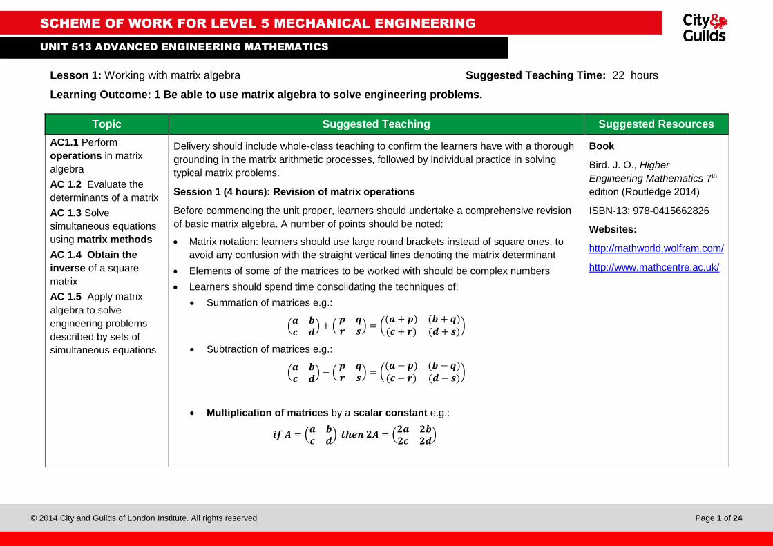
Delivery should include whole-class teaching to confirm the learners have with a thorough

grounding in the matrix arithmetic processes, followed by individual practice in solving

typical matrix problems.

Session 1 (4 hours): Revision of matrix operations

Before commencing the unit proper, learners should undertake a comprehensive revision

of basic matrix algebra. A number of points should be noted:

Matrix notation: learners should use large round brackets instead of square ones, to

avoid any confusion with the straight vertical lines denoting the matrix determinant

Elements of some of the matrices to be worked with should be complex numbers

Learners should spend time consolidating the techniques of:

Summation of matrices e.g.:

(𝒂 𝒃𝒄 𝒅

) + ( 𝒑 𝒒𝒓 𝒔

) = ((𝒂 + 𝒑) (𝒃 + 𝒒)(𝒄 + 𝒓) (𝒅 + 𝒔)

)

Subtraction of matrices e.g.:

(𝒂 𝒃𝒄 𝒅

) − ( 𝒑 𝒒𝒓 𝒔

) = ((𝒂 − 𝒑) (𝒃 − 𝒒)(𝒄 − 𝒓) (𝒅 − 𝒔)

)

Multiplication of matrices by a scalar constant e.g.:

𝒊𝒇 𝑨 = (𝒂 𝒃𝒄 𝒅

) 𝒕𝒉𝒆𝒏 𝟐𝑨 = (𝟐𝒂 𝟐𝒃𝟐𝒄 𝟐𝒅

)

Book

Bird. J. O., Higher

Engineering Mathematics 7th

edition (Routledge 2014)

ISBN-13: 978-0415662826

Websites:

http://mathworld.wolfram.com/

http://www.mathcentre.ac.uk/










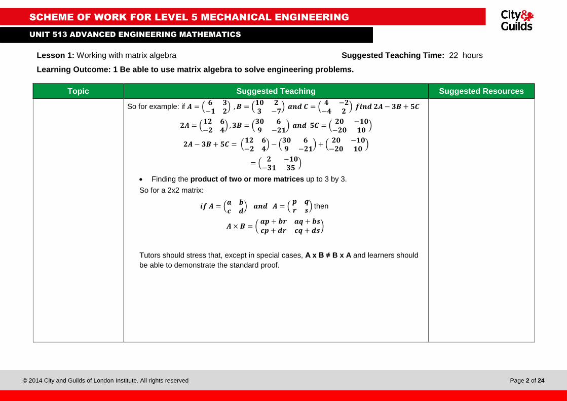
So for example: if 𝑨 = (𝟔 𝟑

−𝟏 𝟐) , 𝑩 = (

𝟏𝟎 𝟐𝟑 −𝟕

) 𝒂𝒏𝒅 𝑪 = (𝟒 −𝟐

−𝟒 𝟐) 𝒇𝒊𝒏𝒅 𝟐𝑨 − 𝟑𝑩 + 𝟓𝑪

𝟐𝑨 = (𝟏𝟐 𝟔−𝟐 𝟒

) , 𝟑𝑩 = (𝟑𝟎 𝟔𝟗 −𝟐𝟏

) 𝒂𝒏𝒅 𝟓𝑪 = (𝟐𝟎 −𝟏𝟎

−𝟐𝟎 𝟏𝟎)

𝟐𝑨 − 𝟑𝑩 + 𝟓𝑪 = (𝟏𝟐 𝟔−𝟐 𝟒

) − (𝟑𝟎 𝟔𝟗 −𝟐𝟏

) + (𝟐𝟎 −𝟏𝟎

−𝟐𝟎 𝟏𝟎)

= (𝟐 −𝟏𝟎

−𝟑𝟏 𝟑𝟓)

Finding the product of two or more matrices up to 3 by 3.

So for a 2x2 matrix:

𝒊𝒇 𝑨 = (𝒂 𝒃𝒄 𝒅

) 𝒂𝒏𝒅 𝑨 = ( 𝒑 𝒒𝒓 𝒔

) then

𝑨 × 𝑩 = ( 𝒂𝒑 + 𝒃𝒓 𝒂𝒒 + 𝒃𝒔𝒄𝒑 + 𝒅𝒓 𝒄𝒒 + 𝒅𝒔

)

Tutors should stress that, except in special cases, A x B ≠ B x A and learners should

be able to demonstrate the standard proof.








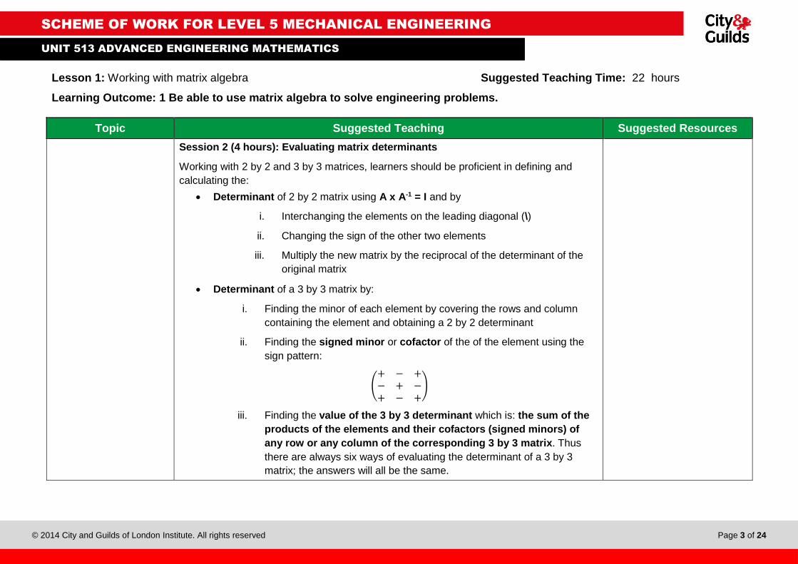
Session 2 (4 hours): Evaluating matrix determinants

Working with 2 by 2 and 3 by 3 matrices, learners should be proficient in defining and

calculating the:

Determinant of 2 by 2 matrix using A x A-1 = I and by

i. Interchanging the elements on the leading diagonal (\)

ii. Changing the sign of the other two elements

iii. Multiply the new matrix by the reciprocal of the determinant of the

original matrix

Determinant of a 3 by 3 matrix by:

i. Finding the minor of each element by covering the rows and column

containing the element and obtaining a 2 by 2 determinant

ii. Finding the signed minor or cofactor of the of the element using the

sign pattern:

(+ − +− + −+ − +

)

iii. Finding the value of the 3 by 3 determinant which is: the sum of the

products of the elements and their cofactors (signed minors) of

any row or any column of the corresponding 3 by 3 matrix. Thus

there are always six ways of evaluating the determinant of a 3 by 3

matrix; the answers will all be the same.








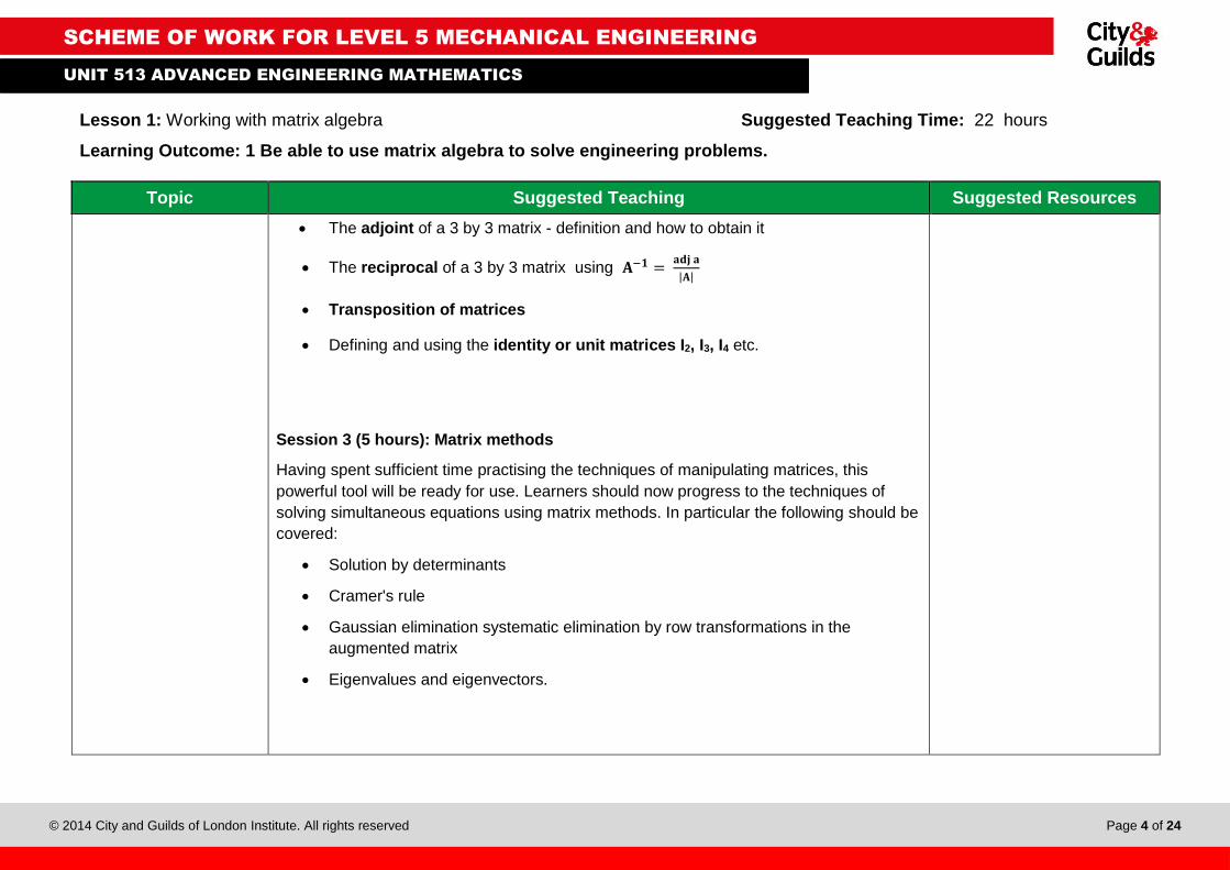
The adjoint of a 3 by 3 matrix - definition and how to obtain it

The reciprocal of a 3 by 3 matrix using 𝐀−𝟏 = 𝐚𝐝𝐣 𝐚

|𝐀|

Transposition of matrices

Defining and using the identity or unit matrices I2, I3, I4 etc.

Session 3 (5 hours): Matrix methods

Having spent sufficient time practising the techniques of manipulating matrices, this

powerful tool will be ready for use. Learners should now progress to the techniques of

solving simultaneous equations using matrix methods. In particular the following should be

covered:

Solution by determinants

Cramer's rule

Gaussian elimination systematic elimination by row transformations in the

augmented matrix

Eigenvalues and eigenvectors.








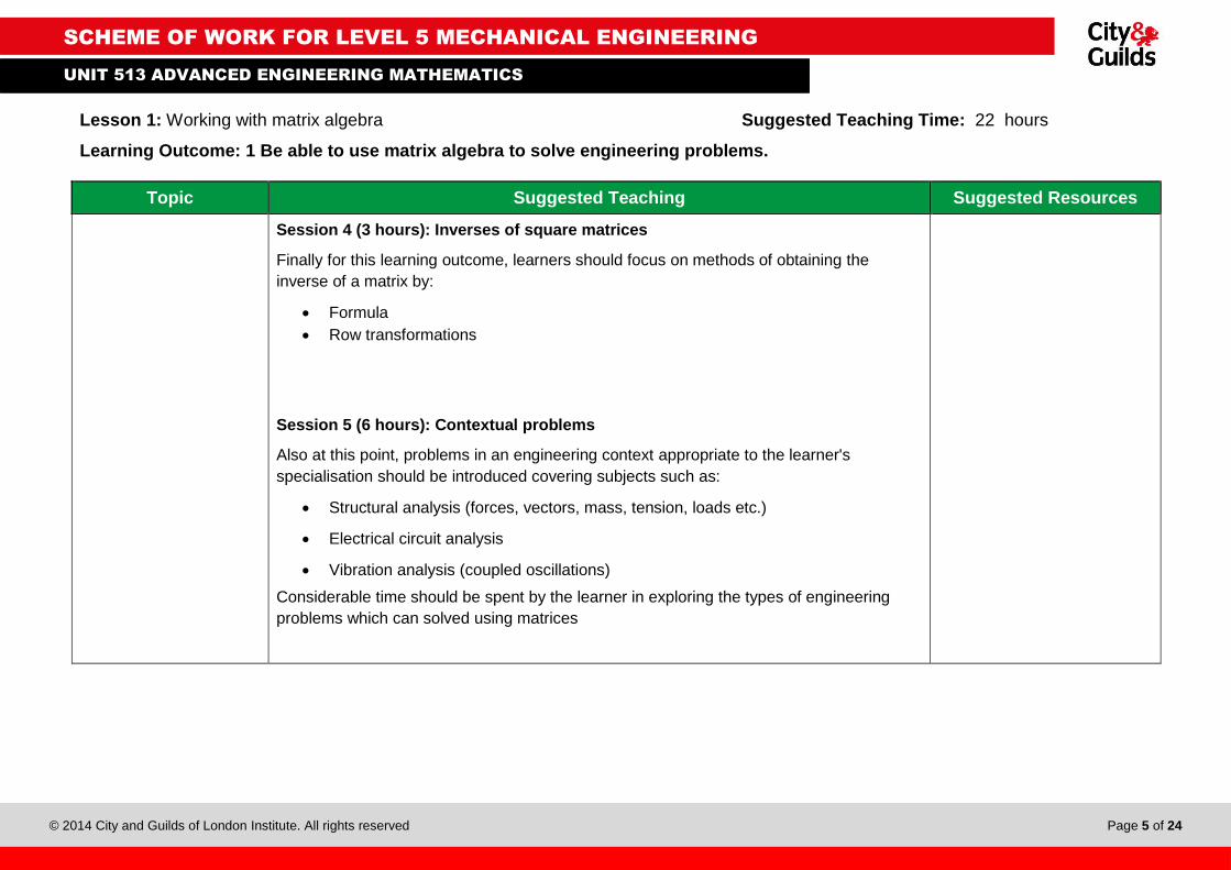
Session 4 (3 hours): Inverses of square matrices

Finally for this learning outcome, learners should focus on methods of obtaining the

inverse of a matrix by:

Formula

Row transformations

Session 5 (6 hours): Contextual problems

Also at this point, problems in an engineering context appropriate to the learner's

specialisation should be introduced covering subjects such as:

Structural analysis (forces, vectors, mass, tension, loads etc.)

Electrical circuit analysis

Vibration analysis (coupled oscillations)

Considerable time should be spent by the learner in exploring the types of engineering

problems which can solved using matrices





Lesson 2: Using vectors Suggested Teaching Time: 10 hours

Learning Outcome: 2. Be able to use vector methods to solve engineering problems


AC 2.1 Perform

operations with

vectors

AC 2.2 Solve

engineering

problems using

vectors

Delivery is likely to be via whole-class teaching initially however the majority of learner activity

will be in group and self-study.

Session 1 (3 hours): Revision of vector and scalar basics

Tutors should ensure firstly that the learners have a good grounding in vector notation and

vector resolution. There should be a period of revision of the following in an engineering context:

Scalar and vector definition

Drawing vectors, including addition by both 'nose to tail' and parallelogram methods

Finding resultants of two or more forces by resolution into horizontal and vertical

components

Addition of vectors by calculation

Subtraction of vectors

Velocity problems

i, j, k notation

Session 2 (3 hours): Vector and scalar products

The learner should then progress to vector and scalar products, with related engineering

problems being introduced as soon as is appropriate. Subjects and techniques which should be

covered are:

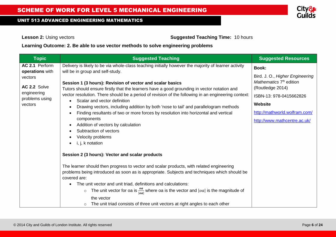
The unit vector and unit triad, definitions and calculations:

o The unit vector for oa is 𝒐𝒂

|𝒐𝒂| where oa is the vector and |𝑜𝑎| is the magnitude of

the vector

o The unit triad consists of three unit vectors at right angles to each other

Book:

Bird. J. O., Higher Engineering

Mathematics 7th edition

(Routledge 2014)

ISBN-13: 978-0415662826

Website












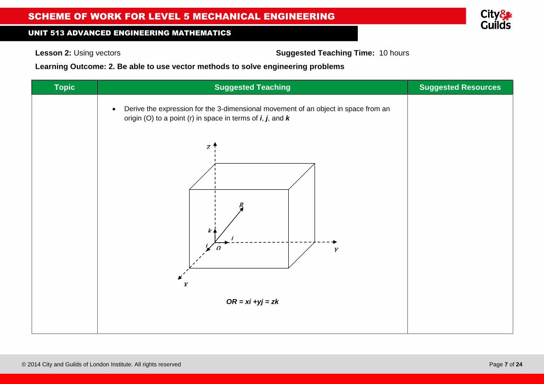
Derive the expression for the 3-dimensional movement of an object in space from an

origin (O) to a point (r) in space in terms of i, j, and k

OR = xi +yj = zk

O

Z

Y

k

X

j i

R








The scalar or dot product of two vectors e.g.: oa ∙ ob = oa ∙ ob ∙ cos(θ2 - θ1) where

θ2 > θ1

Vector or cross product: |𝒐𝒂 ∙ 𝒐𝒃| = 𝒐𝒂 ∙ 𝒐𝒃 ∙ 𝒔𝒊𝒏𝜽

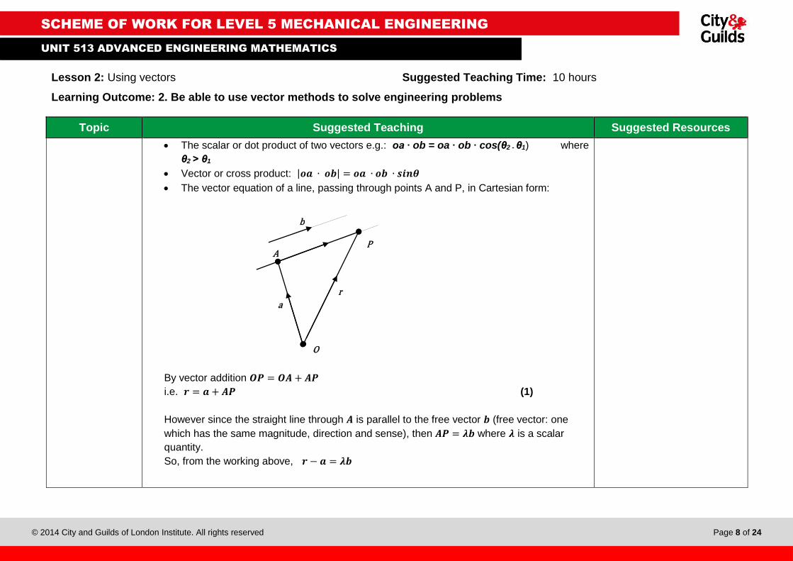
The vector equation of a line, passing through points A and P, in Cartesian form:

By vector addition 𝑶𝑷 = 𝑶𝑨 + 𝑨𝑷

i.e. 𝒓 = 𝒂 + 𝑨𝑷 (1)

However since the straight line through 𝑨 is parallel to the free vector 𝒃 (free vector: one

which has the same magnitude, direction and sense), then 𝑨𝑷 = 𝝀𝒃 where 𝝀 is a scalar

quantity.

So, from the working above, 𝒓 − 𝒂 = 𝝀𝒃

b

P

r

O

A

a








Assume that 𝑟 = 𝑥𝒊 + 𝑦𝒋 + 𝑧𝒌, 𝑎 = 𝑎1𝒊 + 𝑎2𝒋 + 𝑎3𝒌 𝑎𝑛𝑑 𝑏 = 𝑏1𝒊 + 𝑏2𝒋 + 𝑏3𝒌 then from

equation (1):

𝑥𝒊 + 𝑦𝒋 + 𝑧𝒌 = (𝑎1𝒊 + 𝑎2𝒋 + 𝑎3𝒌) + 𝝀 (𝑏1𝒊 + 𝑏2𝒋 + 𝑏3𝒌)

𝒙 − 𝒂𝟏

𝒃𝟏=

𝒚 − 𝒂𝟐

𝒃𝟐=

𝒛 − 𝒂𝟑

𝒃𝟑= 𝝀

So 𝑥 = 𝑎1 + 𝜆𝑏1, 𝑦 = 𝑎2 + 𝜆𝑏2 and 𝑧 = 𝑎3 + 𝜆𝑏3

Solving for 𝜆 gives:

𝒙 − 𝒂𝟏

𝒃𝟏=

𝒚 − 𝒂𝟐

𝒃𝟐=

𝒛 − 𝒂𝟑

𝒃𝟑= 𝝀

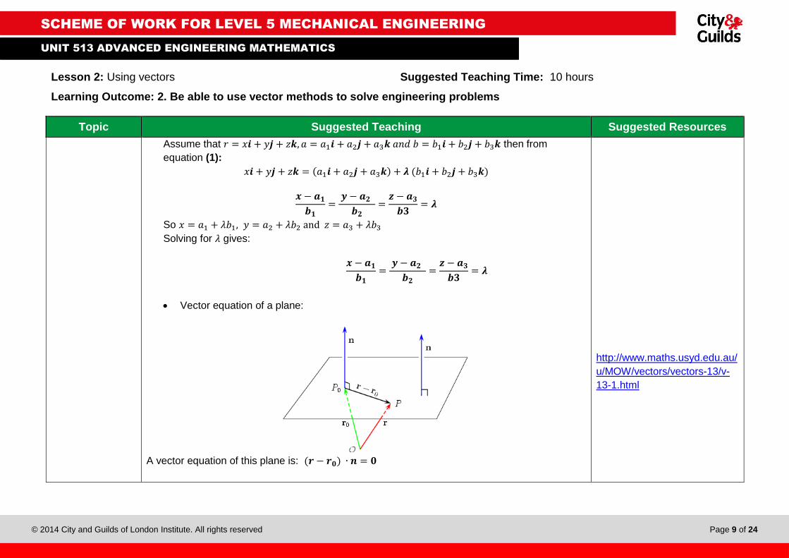
Vector equation of a plane:

A vector equation of this plane is: (𝒓 − 𝒓𝟎) ∙ 𝒏 = 𝟎

http://www.maths.usyd.edu.au/

u/MOW/vectors/vectors-13/v-

13-1.html

http://www.maths.usyd.edu.au/u/MOW/vectors/vectors-13/v-13-1.html










Session 3 (4 hours): Engineering vector problems

There should be a period of practice of a rage of set engineering problems involving the use of

the above, until the learner feels confident in solving them. Subjects could include fluid or gas

flow, stresses, strains and displacements in structures, and deformation of materials. This may

only take a short time it the learner has recently progressed from a lower level of engineering

mathematics.





Lesson 3: Partial differentiation, integration and differential equations Suggested Teaching Time: 10 hours

Learning Outcome: 3. Be able to use calculus to solve engineering problems

4. Be able to apply numerical analysis to solve engineering problems


AC 3.1 Evaluate partial

derivatives for a

function of several

variables

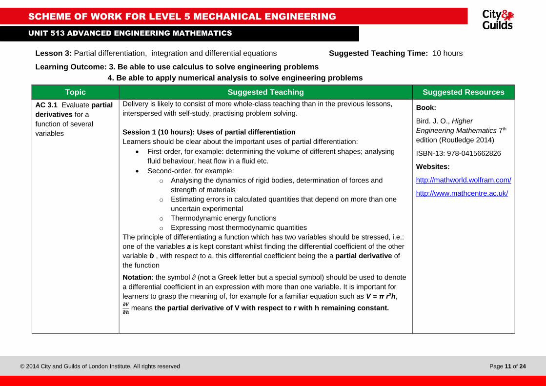
Delivery is likely to consist of more whole-class teaching than in the previous lessons,

interspersed with self-study, practising problem solving.

Session 1 (10 hours): Uses of partial differentiation

Learners should be clear about the important uses of partial differentiation:

First-order, for example: determining the volume of different shapes; analysing

fluid behaviour, heat flow in a fluid etc.

Second-order, for example:

o Analysing the dynamics of rigid bodies, determination of forces and

strength of materials

o Estimating errors in calculated quantities that depend on more than one

uncertain experimental

o Thermodynamic energy functions

o Expressing most thermodynamic quantities

The principle of differentiating a function which has two variables should be stressed, i.e.:

one of the variables a is kept constant whilst finding the differential coefficient of the other

variable b , with respect to a, this differential coefficient being the a partial derivative of

the function

Notation: the symbol ∂ (not a Greek letter but a special symbol) should be used to denote

a differential coefficient in an expression with more than one variable. It is important for

learners to grasp the meaning of, for example for a familiar equation such as V = π r2h, 𝝏𝑽

𝝏𝒉 means the partial derivative of V with respect to r with h remaining constant.

Book:

Bird. J. O., Higher



ISBN-13: 978-0415662826

Websites:













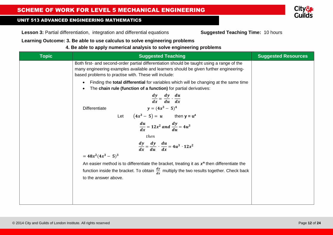
Both first- and second-order partial differentiation should be taught using a range of the

many engineering examples available and learners should be given further engineering-

based problems to practise with. These will include:

Finding the total differential for variables which will be changing at the same time

The chain rule (function of a function) for partial derivatives:

𝒅𝒚

𝒅𝒙=

𝒅𝒚

𝒅𝒖 ∙

𝒅𝒖

𝒅𝒙

Differentiate 𝒚 = (𝟒𝒙𝟑 − 𝟓)𝟒

Let (𝟒𝒙𝟑 − 𝟓) = 𝒖 then y = u4

𝒅𝒖

𝒅𝒙= 𝟏𝟐𝒙𝟐 𝒂𝒏𝒅

𝒅𝒚

𝒅𝒖= 𝟒𝒖𝟑

𝑡ℎ𝑒𝑛

𝒅𝒚

𝒅𝒙=

𝒅𝒚

𝒅𝒖 ∙

𝒅𝒖

𝒅𝒙= 𝟒𝒖𝟑 ∙ 𝟏𝟐𝒙𝟐

= 𝟒𝟖𝒙𝟐(𝟒𝒙𝟑 − 𝟓)𝟑

An easier method is to differentiate the bracket, treating it as 𝒙𝒏 then differentiate the

function inside the bracket. To obtain 𝒅𝒚

𝒅𝒙 multiply the two results together. Check back

to the answer above.









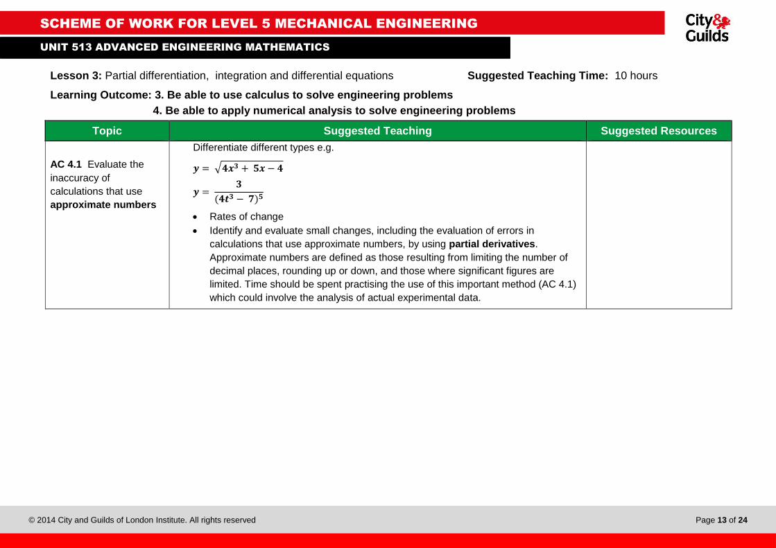
AC 4.1 Evaluate the

inaccuracy of

calculations that use

approximate numbers

Differentiate different types e.g.

𝒚 = √𝟒𝒙𝟑 + 𝟓𝒙 − 𝟒

𝒚 = 𝟑

(𝟒𝒕𝟑 − 𝟕)𝟓

Rates of change

Identify and evaluate small changes, including the evaluation of errors in

calculations that use approximate numbers, by using partial derivatives.

Approximate numbers are defined as those resulting from limiting the number of

decimal places, rounding up or down, and those where significant figures are

limited. Time should be spent practising the use of this important method (AC 4.1)

which could involve the analysis of actual experimental data.





Lesson 4: Series and transforms Suggested Teaching Time: 22 hours




AC 3.2 Use series

expansions to obtain

approximations of a

function

Delivery is likely to be by continued whole class teaching mixed with self study and

practice in problem solving. The syllabus could be taught in one of two sequences -

following the ACs in order, or each of the subjects could be followed through by combining

the ACs in an appropriate sequence. The following is a version of the latter.

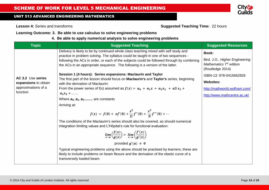
Session 1 (4 hours): Series expansions: Maclaurin and Taylor

The first part of the lesson should focus on Maclaurin's and Taylor's series, beginning

with the derivation of Maclaurin:

From the power series of f(x) assumed as 𝒇(𝒙) = 𝒂𝟎 + 𝒂𝟏𝒙 + 𝒂𝟐𝒙𝟐 + 𝒂𝟑 𝒙𝟑 +

𝒂𝟒𝒙𝟒 +. . . . . .

Where a0, a1, a2......... are constants

Arriving at:

𝒇(𝒙) = 𝒇(𝟎) + 𝒙𝒇′(𝟎) +𝒙𝟐

𝟐!𝒇′′(𝟎) +

𝒙𝟑

𝟑!𝒇′′′(𝟎) + ⋯

The conditions of the Maclaurin's series should also be covered, as should numerical

integration limiting values and L'Hôpital’s rule for functional evaluation:

𝒍𝒊𝒎𝒙→𝒂

(𝒇(𝒙)

𝒈(𝒙)) = 𝒍𝒊𝒎

𝒙→𝒂(

𝒇′(𝒙)

𝒈′(𝒙))

provided 𝒈′(𝒂) ≠ 𝟎

Typical engineering problems using the above should be practised by learners; these are

likely to include problems on beam flexure and the derivation of the elastic curve of a

transversely loaded beam.

Book:

Bird. J.O., Higher Engineering

Mathematics 7th edition

(Routledge 2014)

ISBN-13: 978-0415662826

Websites:













AC 4.2 Use numerical

iterative methods to

find the roots of a

function

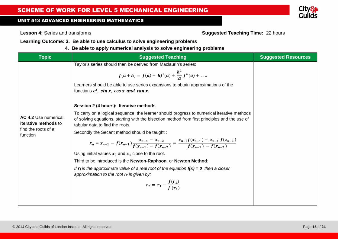
Taylor's series should then be derived from Maclaurin's series:

𝒇(𝒂 + 𝒉) = 𝒇(𝒂) + 𝒉𝒇′(𝒂) + 𝒉𝟐

𝟐! 𝒇′′(𝒂) + … ..

Learners should be able to use series expansions to obtain approximations of the

functions 𝒆𝒙, 𝒔𝒊𝒏 𝒙, 𝒄𝒐𝒔 𝒙 𝒂𝒏𝒅 𝒕𝒂𝒏 𝒙.

Session 2 (4 hours): Iterative methods

To carry on a logical sequence, the learner should progress to numerical iterative methods

of solving equations, starting with the bisection method from first principles and the use of

tabular data to find the roots.

Secondly the Secant method should be taught :

𝒙𝒏 = 𝒙𝒏−𝟏 − 𝒇(𝒙𝒏−𝟏 )𝒙𝒏−𝟏 − 𝒙𝒏−𝟐

𝒇(𝒙𝒏−𝟏 ) − 𝒇(𝒙𝒏−𝟐 ) =

𝒙𝒏−𝟐𝒇(𝒙𝒏−𝟏 ) − 𝒙𝒏−𝟏 𝒇(𝒙𝒏−𝟐 )

𝒇(𝒙𝒏−𝟏 ) − 𝒇(𝒙𝒏−𝟐 )

Using initial values 𝒙𝟎 and 𝒙𝟏 close to the root.

Third to be introduced is the Newton-Raphson, or Newton Method:

If r1 is the approximate value of a real root of the equation f(x) = 0 then a closer

approximation to the root r2 is given by:

𝒓𝟐 = 𝒓𝟏 − 𝒇(𝒓𝟏)

𝒇′(𝒓𝟏)









AC 3.3 Obtain a Fourier

series description for

functions of a single

variable

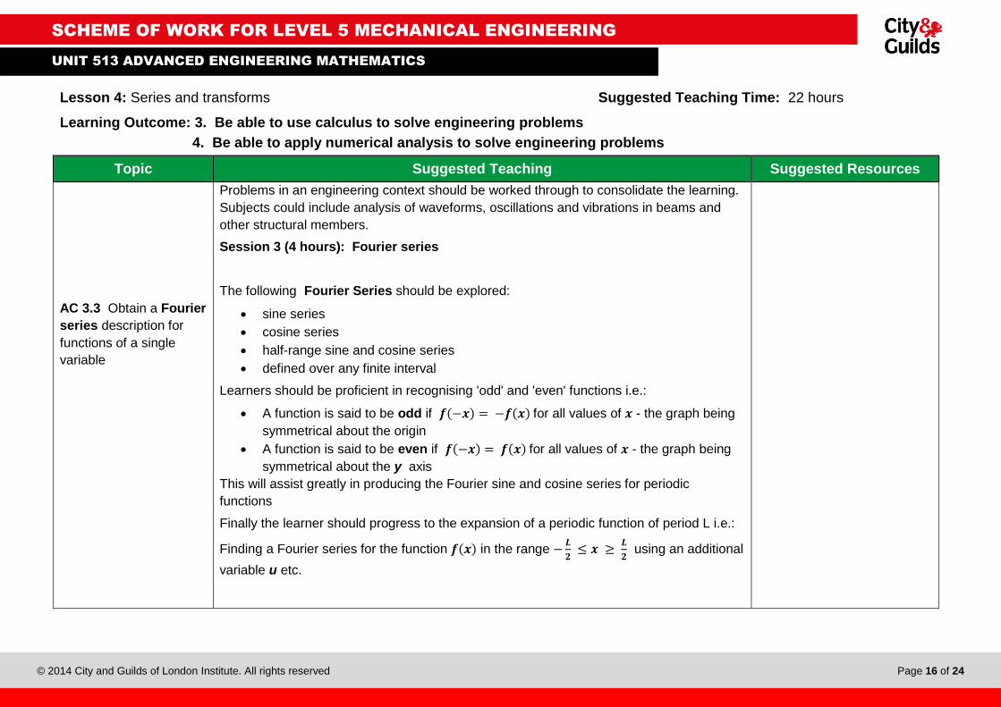
Problems in an engineering context should be worked through to consolidate the learning.

Subjects could include analysis of waveforms, oscillations and vibrations in beams and

other structural members.

Session 3 (4 hours): Fourier series

The following Fourier Series should be explored:

sine series

cosine series

half-range sine and cosine series

defined over any finite interval

Learners should be proficient in recognising 'odd' and 'even' functions i.e.:

A function is said to be odd if 𝒇(−𝒙) = −𝒇(𝒙) for all values of 𝒙 - the graph being

symmetrical about the origin

A function is said to be even if 𝒇(−𝒙) = 𝒇(𝒙) for all values of 𝒙 - the graph being

symmetrical about the y axis

This will assist greatly in producing the Fourier sine and cosine series for periodic

functions

Finally the learner should progress to the expansion of a periodic function of period L i.e.:

Finding a Fourier series for the function 𝒇(𝒙) in the range −𝑳

𝟐 ≤ 𝒙 ≥

𝑳

𝟐 using an additional

variable u etc.









AC 3.4 Obtain Laplace

transforms for simple

functions

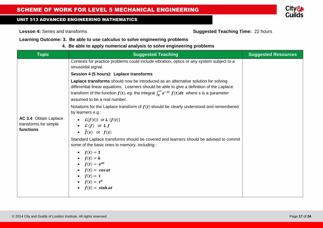
Contexts for practice problems could include vibration, optics or any system subject to a

sinusoidal signal.

Session 4 (5 hours): Laplace transforms

Laplace transforms should now be introduced as an alternative solution for solving

differential linear equations. Learners should be able to give a definition of the Laplace

transform of the function 𝒇(𝒕), eg: the integral ∫ 𝒆−𝒔𝒕∞

𝟎 𝒇(𝒕)𝒅𝒕 where s is a parameter

assumed to be a real number.

Notations for the Laplace transform of 𝒇(𝒕) should be clearly understood and remembered

by learners e.g.:

𝓛{𝒇(𝒕)} or L {𝒇(𝒕)}

𝓛 (𝒇) or L 𝒇

𝒇(𝒔) or 𝒇(𝒔)

Standard Laplace transforms should be covered and learners should be advised to commit

some of the basic ones to memory, including :

𝒇(𝒕) = 𝟏

𝒇(𝒕) = 𝒌

𝒇(𝒕) = 𝒆𝒂𝒕

𝒇(𝒕) = 𝐜𝐨𝐬 𝒂𝒕

𝒇(𝒕) = 𝒕

𝒇(𝒕) = 𝒕𝒏

𝒇(𝒕) = 𝐬𝐢𝐧𝐡 𝒂𝒕









AC 3.5 Obtain the

inverse Laplace

transforms for simple

functions

Providing the learners with a list of elementary standard Laplace transforms will be useful

e.g.:

http://www.mathcentre.ac.uk/resources/uploaded/43799-maths-centre-more-ff-for-web.pdf

which also gives data for other topics in this unit

Session 5 (5 hours): Inverse Laplace transforms

Learners should spend some time on worked examples of Laplace transforms before

moving on to inverse Laplace transforms.

Again, time should be spent on worked examples of inverse Laplace transforms

involving simple functions until learners are confident and proficient, remembering that

these are tools with which they should become very familiar.

Learners must be able to obtain inverse Laplace transforms for:

Algebraic functions between the limits t = 0 and s = ∞

and

Trigonometric functions between limits -π and π.

Finally on this topic the learner should apply the Laplace transform to the Unit Step or

Heaviside function, and the basic theory and solution of the Dirac delta

function/distribution. These deal with sudden inputs to a system of indefinite duration, and

the characteristics of a sudden 'spike' input. Worked examples from different engineering

concepts such as electrical switching, impacts, sudden accelerations, the application of the

brakes of a moving vehicle and the sudden acceleration and deceleration of a rotating

shaft such as in a vehicle transmission.

http://www.mathcentre.ac.uk/resources/uploaded/43799-maths-centre-more-ff-for-web.pdf





Lesson 5: Numerical methods of integration and solving differential equations Suggested Teaching Time: 21 hours




AC 3.6 Obtain integrals

of simple functions

Session 1 (4 hours): Integrals of simple functions

Delivery, once again, is likely to consist of whole-class teaching interspersed with self-

study to practise problem solving. However as learners become more proficient at using

the techniques from this and other lessons, they could be divided into groups and be given

more complex engineering problems to solve as a team.

Returning to calculus, the final lesson in the unit starts with the integration of simple

functions. Learners are likely to have worked with integration previously, however it will do

no harm at all to revise the basics.

The idea of integration as the reverse of differentiation, and also of a process of

summation are important and the learner be familiar with the basic rules of these

processes. The meaning of the notation should be clear also e.g.: ∫ 𝟐𝒙 𝒅𝒙 + c means 'the

integral of 𝟐𝒙 with respect to 𝒙, and c denotes the possible presence of a constant. Also

the standard integrals for common functions should be studied and as many as possible

committed to memory, particularly the integrals of a constant,

𝒂𝒙𝒏 (𝒘𝒉𝒆𝒓𝒆 𝒏 ≠ −𝟏, 𝟏

𝒙 , 𝐬𝐢𝐧 (𝒂𝒙 ± 𝒃), 𝐜𝐨𝐬(𝒂𝒙 ± 𝒃) 𝒂𝒏𝒅 𝒆(𝒂𝒙±𝒃)

The concept of limits and evaluating the integral between them should be learned and

practised with all of the standard functions. The learner should also clearly understand

the difference between an indefinite integral i.e. one containing the constant 'c' and a

definite integral i.e. one in which limits have been applied. At this stage, engineering

context can be introduced; the learner should be able to solve problems involving, for

instance, entropy change, volume of gas or liquid in a container, or voltage waveforms.

Learners should be able to find the mean and Root Mean Square (RMS) values of a

waveform.

Book:

Bird. J. O., Higher



ISBN-13: 978-0415662826

Websites:













AC 4.3 Apply numerical

methods of integration

to engineering

variables

Session 2 (4 hours): Numerical methods of integration

Numerical methods of integration are important and the learner should be able to apply

two rules Trapezoidal rule and Simpson's rule:

The Trapezoidal rule: for those learners who are unfamiliar with the use of this rule, it is

best to start with the arithmetical method of finding the area under an irregular curve.

Dividing the area between the curve and the x - y axes into a number of thin strips, each of

which approximates to a trapezoid. The area bounded by the curve and the x - y axes is

given by :

(Interval width) [½ (first + last ordinate) + sum of remaining ordinates]

Quickly progressing then to numerical integration, the learner will see that the above is

equal to ∫ 𝒚𝒅𝒙𝒃

𝒂 . Learners should be able to write down the standard proof of this from

memory, and apply the rule to any problem. This applies also to the related Mid-ordinate

rule.

Simpson's rule follows on from the preceding two but is a more accurate approximation;

learners should always encouraged to think in terms of errors, how they can be reduced in

their calculations and how they affect the calculation if they can't be eliminated. Learners

should be able to demonstrate how the rule works and how it is derived, including the fact

that it only works with an even number of intervals (odd number of ordinates).









AC 3.7 Solve ordinary

differential equations

Engineering-based problems should be practised by the learners, in a range of contexts,

which could include fluid flow rates, vibration, distortion of a body or structure under its

own weight, spread of a contaminant in a water course or fluid system. In fact any physical

property where data are only available at discrete points or intervals.

Work with differential equations may be revision for the members of the class, but, as

always, there will be those who have not remembered the rules and methods as well as

the others. So it is often helpful to revise the families of curves, the notation and the basic

rules of differentiation and solving differential equations by separation of variables.

Session 3 (4 hours): First-order ordinary differential equations (AC 3.7 & 4.4)

Learners should be able to recognise and to readily solve first-order differential equations

of the following forms:

𝒅𝒚

𝒅𝒙= 𝒇(𝒙)

𝒅𝒚

𝒅𝒙= 𝒇(𝒚)

𝒅𝒚

𝒅𝒙= 𝒇(𝒙) ∙ 𝒇(𝒚)

Problems in an engineering context could be introduced here.









AC 4.4 Apply

numerical methods for

the solution of ordinary

differential equation

models of engineering

systems

Solving exact first-order differential equations: learners should be able to define and

solve exact first-order differential equations by partial differentiation, and should also be

able to test a given equation for exactness.

Solving linear first-order differential equations: learners should be able to define and

recognise a first-order linear differential equation and to solve, using an integrating factor,

equations of the form:

𝒅𝒚

𝒅𝒙 + 𝑷𝒚 = 𝑸 where 𝑷 and 𝑸 are functions of 𝒙 only

Learners should practise solving problems in an engineering context, which could include:

equations of motion of particles in a resisting fluid, alternating current, impurities in an

engine oil tank etc.

Session 4: Second-order ordinary differential equations (AC 3.7 & 4.4)

Learners should be able to identify the types of engineering problem that can be solved

using the methods to be addressed in this part of the lesson. These include: free vibration

analysis with mass-spring systems, resonant and non-resonant vibration analysis,

mechanical and fluid-induced vibration etc.

Learners should be familiar with the D-operator and its use and should be able to identify

homogeneous and non-homogeneous differential equations. And should be proficient in

solving equations of the form:

𝒂𝒅𝟐𝒚

𝒅𝒙𝟐+ 𝒃

𝒅𝒚

𝒅𝒙+ 𝒄𝒚









AC 4.5 Apply iterative

numerical methods to

the solution of partial

differential equation

models of engineering

systems

Finding the complementary function (C.F.) using the D-operator and the particular

integral (P.I.) using trial functions. This results in the general solution of the above

equation: 𝒚 = 𝑪. 𝑭. ∙ 𝑷. 𝑰.

Particular integrals should be a focus for learners and they should be encouraged to

commit at least some to memory.

Learners should understand and be able to apply the procedure for solving ordinary

differential equations using Laplace transforms.

Practice examples should include those involving initial and boundary values, those

involving sinusoidal inputs (i.e.: the response of a system to sinusoidal inputs), and those

involving resonance.

Session 5 (5 hours): Iterative numerical methods

The final part of the unit involves numerical methods for solving ordinary and partial

differential equation models of engineering systems. Examples should cover a range of

relevant systems. Learners should approach each method one by one, where appropriate

comparing the results and procedures for individual equations.

Starting with ordinary differential equations, the contextual problems should centre

particularly around areas, volumes, centres of gravity and moments of inertia. Methods to

be addressed by the learners are:

Euler: taking the first two terms of the Taylor series:

𝒇(𝒂 + 𝒉) = 𝒇(𝒂) + 𝒉𝒇′(𝒂)









Euler-Cauchy: learners should be able to demonstrate the difference in accuracy

between this and the standard Euler method

Taylor series

Runge-Kutta: learners should not be expected to derive or prove this method,

however they should be able to follow the seven steps in order to arrive at a highly

accurate solution to an equation.

Finite difference: forward, backward and central

It would be a useful exercise for learners to construct a table of solutions for a particular

equation, say 𝒚 = 𝒙 + 𝟏 + 𝒆𝒙 using each of the above methods to compare their

accuracies. This will help the learner to remember the relative accuracies and to be able to

select an appropriate method for a particular problem.

The final subject in this unit is the solution of partial differential equation models of

engineering systems using iterative numerical methods. The following should be

included:

Finite difference methods (similar to above)

The Jacobi1 iterative method for a square set of linear equations: Ax = b

The Gauss-Seidel1 iterative method for a square set of linear equations: Ax = b

Learners should then complete a series of problems based on typical and relevant

engineering systems. The aim is to consolidate all of the unit learning and to give learners

practice in selecting and using methods taught in the unit.

1 These two methods do not appear in the recommended textbook, but can be found on the Wolfram.com website

Documents

SCHEME OF WORK FOR LEVEL 5 MECHANICAL ENGINEERING … · SCHEME OF WORK FOR LEVEL 5 MECHANICAL ENGINEERING Scheme of woOW LEVEL 3 Engineering UNIT 513 ADVANCED ENGINEERING MATHEMATICS