Schlieren VisualizationAe 104b

TA: Bryan SchmidtLab: T5 (Guggenheim 407)bsschmid@caltech.edu

Winter 2015

1 Goals of the experiment

In this experiment you will assemble and align a schlieren/shadowgraph setup from components in theCann Laboratory and use it to visualize phenomena in fluids and solids using a high-speed camera. Uponcompletion of this experiment, you should:

• Have a fundamental understanding of the theory of schlieren and shadowgraph visualization techniques

• Have a working knowledge of schlieren and shadowgraph setups including placement and alignmentof optics and practical issues involved with the individual components involved: mirrors, light source,cutoff, focusing optics, and camera. Given components, you should be able to set up your own schlierenor shadowgraph system

• Understand what types of phenomena are good candidates for schlieren and shadowgraph visualization

2 Basic principles

This project deals with schlieren and shadowgraph visualization techniques, which translate phase speeddifferences in light, invisible to the eye, into changes in intensity which we perceive as regions of light anddark. A brief discussion of these techniques is presented here; for a more complete description the readeris referred to the famous book by Settles [1]. Change in phase speed as light passes through a transparentmedium is called refraction. The refractive index n = c0/c of a medium describes the change in phase speedwhere c is the speed of light in the medium and c0 is the speed of light in a vacuum. For gases the refractiveindex is linearly dependent on the gas density according to the Gladstone-Dale relation:

n = Kρ+ 1 (1)

where K is the Gladstone-Dale constant and ρ is the gas density. K is dependent on gas composition,temperature, and the wavelength of the light passing through the medium. In gases K is typically between0.1×10−3 and 1.5×10−3 (kg/m3)−1. Kρ is therefore much smaller than 1, so the refractive index varies onlyin the third or fourth decimal place. Hence very sensitive optics are required to detect changes in densityin gases. Gas flows with changing density are collectively called compressible flows, and compressibility canbe produced by temperature variations and/or appreciable Mach number such that M2 is not substantially

1

Ae104b, Winter 2014 Schlieren Visualization

smaller than 1. Refractive indices of transparent liquids and solids are much higher than those of gases, somuch less optical sensitivity is required to observe refractions in liquids or solids than gases [1].

A light ray passing orthogonally through a change in refractive index will experience a change in phasevelocity but will continue traveling in the same direction. If the light ray intersects the change in refractiveindex obliquely, however, it will bend towards the region with greater n. For a light ray travelling in thez-direction intersecting a region of varying refractive index the ray curvature is given by

∂2x

∂z2=

1

n

∂n

∂x(2)

Here x is used to represent a direction orthogonal to the ray propagation. Integrating once, the angular raydeflection is

ε =1

n

∫∂n

∂x∂z (3)

From Equation 3 we see that ray deflection is dependent not only on the refractive index of the mediumbut mainly on the gradients in n orthogonal to the ray propagation direction. Because of the integral inz, deflection is also quite sensitive to the extent of the region of varying density in the z-direction. Thesedeflections are what are made visible by schlieren and shadowgraph techniques.

2.1 Shadowgraph

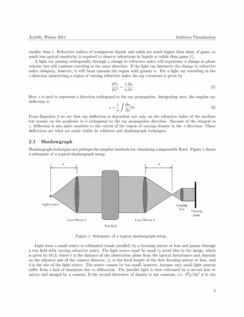
Shadowgraph techniques are perhaps the simplest methods for visualizing compressible flows. Figure 1 showsa schematic of a typical shadowgraph setup.

Figure 1: Schematic of a typical shadowgraph setup.

Light from a small source is collimated (made parallel) by a focusing mirror or lens and passes througha test field with varying refractive index. The light source must be small to avoid blur in the image, whichis given by ld/f1 where l is the distance of the observation plane from the optical disturbance and dependson the physical size of the camera detector, f1 is the focal length of the first focusing mirror or lens, andd is the size of the light source. The source cannot be too small, however, because very small light sourcessuffer from a lack of sharpness due to diffraction. The parallel light is then refocused by a second lens ormirror and imaged by a camera. If the second derivative of density is not constant, i.e. ∂3ρ/∂y3 6= 0, the

2

Ae104b, Winter 2014 Schlieren Visualization

Figure 2: Schematic showing the refraction of light rays by density fields with density and its first, second,and third derivatives constant. The two-dimensional description is easily extended to three dimensions.

region where this occurs will appear dark, or as a shadow. Figure 2 illustrates the creation of shadows froma non-constant second derivative in density.

Shadowgraphs are typically used to study shocks and Prandtl-Meyer expansions as both of these flowfeatures create non-constant second derivatives in density. Shadowgraphs are also useful for imaging bound-ary layers and turbulent flows. Shadowgraphs have an advantage over schlieren setups for such flows becauseshadowgraph visualization is uniformly sensitive in all directions. Figure 3 shows a typical shadowgraphimage.

Figure 3: Shadowgraph image of a bullet in supersonic flow. The bow shock is clearly visible as a dark line,as are other weaker shocks and the turbulent wake behind the bullet.

2.2 Schlieren

Schlieren visualization is similar to the shadowgraph technique, but the primary difference is that whileshadowgraphs are sensitive to changes in the second derivative in density, schlieren systems detect changes

3

Ae104b, Winter 2014 Schlieren Visualization

to the first derivative in density. A schlieren setup is nearly identical to that of a shadowgraph but with theaddition of a knife edge at the focal point of the second lens or mirror as shown in Figure 4. The amount oflight blocked by the knife edge is commonly referred to as “cutoff.”

Figure 4: Schematic of a typical schlieren setup.

Undeflected light rays are affected uniformly by the knife edge and the intensity of the image is reducedwith increased cutoff. As light passes through a density field with a non-constant first derivative, the lightrays are deflected as shown in Figure 2. If light rays are deflected towards the knife edge, the part of theimage where those light rays originate from will be darkened more than a part of the image with constantdensity. Conversely, if light rays are deflected away from the knife edge, that part of the image will appearbrighter than unaffected regions of the image. Thus schlieren setups are only sensitive to density gradientsnormal to the knife edge. An example schlieren image is shown in Figure 5. Notice in this image that thebrightness of waves appears reversed in the top and bottom of the image. This is a common feature of manyschlieren images because light is being deflected in opposite directions by gradients on the top and bottomof the model.

The primary advantage of schlieren visualization over shadowgraph visualization is that of sensitivity. Thesensitivity of a shadowgraph setup depends primarily upon optical path length, which is typically difficultand expensive to modify. The sensitivity of a schlieren setup, however, mainly depends on the amountof cutoff used. Higher cutoff leads to decreased brightness in the image, so increased sensitivity comes atthe cost of necessitating a more powerful light source. A related tradeoff exists for the camera. Increasedexposure time increases the brightness of the image but reduces the ability to observe transient phenomenalike nonsteady waves or turbulence in the flow.

In practice, many variations of the basic schlieren setup described here are used. By far the most commonis the Z-type schlieren setup, an almost universal standard. Focusing mirrors provide a much larger fieldof view for the same price as focusing lenses, so the setup is bent into a “Z” shape to utilize the mirrors.Besides the cost advantage, this also saves space in the laboratory. A Z-type schlieren setup does comeat a price, however. The nonlinear alignment of the optics create two effects that distort the image, comaand astigmatism. Coma can be eliminated by careful arrangement and alignment of the focusing mirrors.Astigmatism cannot be fully eliminated, but by using a slit light source aligned with the knife edge it canbe minimized until it is no longer visible. For more information on this, see Settles [1]. Other variationstypically involve the knife edge, such as using a circular or double knife edge to eliminate the reversal inbrightness of conventional schlieren images. Circular knife edges have the added benefit of being sensitive to

4

Ae104b, Winter 2014 Schlieren Visualization

Figure 5: Schlieren image of a wedge in supersonic flow. Notice the difference in the appearance of shocksand other waves between the schlieren image and the shadowgraph.

density gradients in all directions. A further modification is to use color strip filters instead of a knife edge,resulting in colored schlieren images with the color corresponding to the strength of the change in densitygradient.

3 Safety considerations and rules

In the first part of the experiment you will be dealing with an open flame. Be very careful not to accidentallyignite anything besides the sterno heater. The gas used for the jet during this laboratory will come froma bottle filled with compressed gas. The bottle is portable and located in the Cann Lab. The bottle isfilled with pressures ranging from 207 to 340 bar (3000 to 5000 psi). Working with gas in that pressurerange can be very hazardous. Besides risks to hearing from the release of high pressure gas, gas bottlescan also readily become extremely dangerous projectiles if the safety valve is broken or damaged. Be verycareful when opening or closing the bottles or any valves connected to the high-pressure line and only doso as directed by your TA. Whenever the bottles need to be changed, do not do it by yourself becausemishandling high-pressure gas bottles can be very dangerous. Ask the TA to do it or do it under the TA’scareful supervision. You will also be dealing with gas in a somewhat-enclosed environment, which can be anasphixiation hazard if the gas is left running. That is why you must only run the jet when you are activelytaking pictures. Ear protection must be worn any time the jet is in operation.

Here are some general guidelines when performing any sort of experiment:

• Always put on necessary safety gear before interacting with the experimental apparatus

• Never work in the laboratory alone or without notifying someone that you are doing so

• Take the time to THINK carefully before performing any steps with potentially hazardous components

The Cann Lab is shared by several experimental groups and there are multiple active experiments in theLab, some of which are parts of other Ae104b modules and some of which are research projects. Do not

5

Ae104b, Winter 2014 Schlieren Visualization

interfere with the setup of any experiments other than the one for the lab that you are working on, andexercise caution when moving in and out of the enclosures of other experiments. Wear any personal protectiveequipment required by the other experiments when doing so. The schlieren experiment is sharing space witha currently inactive photoelasticity experiment, but the components for the photoelasticity experiment arenot to be touched unless you are told to do so by your TA.

4 Experimental Tasks

The experiment is divided into four separate tasks:

1. Assembly and alignment of the visualization system

2. Visualizaiton of a flame from a sterno heater

3. Visualization of an under-expanded jet

4. Visualization of a phenomena of your choice

4.1 Assembly and alignment

The first task is to assemble and align the schlieren setup. This may seem tedious and might take some timeto attain good alignment and focus, but a well-aligned setup will make all the difference. The instructionshere are a summary of Chapter 8 of Settles [1]; the reader is referred there for a much more complete guide.Chapter 7 also contains some useful tips.

The primary components for the schlieren setup in this experiment are two 4.25-inch (108 mm) diameterf/10 spherical focusing mirrors. The “f-number” of a mirror is the ratio of the focal length to the diameterof the mirror. These mirrors have a focal length of 45 inches (114 cm). Figure 6 shows a to-scale sketch of arecommended layout for the optics. A functional overall length for the system based on the mirrors and thespace available on the optical table is 2 m (78.75”). This length does not need to be exact. A recommendedentrance/exit angle for the beams is somewhere between 2θ = 15◦ and 2θ = 20◦, as shown in the figure.This also does not need to be exact, but it is crucial that the system is symmetric.

Begin by marking off an open 2 m-length on the optical table with tape. It is best to measure some anglebetween 15 and 20 degrees relative to the holes on the optical table for this line to make the alignment ofother optics easier. Place the two mirrors at opposite ends of the tape, facing each other with the surfaceof each mirror coincident with an end of the tape. The mirrors will need to be raised off the table in orderto make their centerline coincide with the height of the light source. Use some of the plastic samples fromthe photoelasticity experiment to do this. Mark the center of the tape to designate the test area. Next,prepare a key instrument for alignment: a clean sheet of white paper. To make alignment easier, drawa 4.25”-diameter circle on the paper to designate the size of the test beam. Assemble the light source ifnecessary. Your TA will give you further instructions on this. Make sure not to exceed the current load ofthe LED. Measure 45” (the focal length of the mirrors) along a row of holes beginning at the surface of thefirst mirror and place the light source there and point it at the first mirror.

At this point it may be helpful to dim the lights in the laboratory or turn them off entirely. Carefullyadjust the distance of the light source from the mirror until the light beam reflected off the first mirror is acircle with 4.25” diameter irrespective of distance from the mirror. This should be tested using the paperprepared earlier. Using the rotation and tilt controls on the first mirror, point the light beam towards thesecond mirror such that the entire second mirror is illuminated. Next measure 45” along a row of holes fromthe second mirror as shown in Figure 6 to form a “Z.” Place the knife-edge at the focus of the second mirrorbut retract it fully below the beam to allow all the light to pass.

6

Ae104b, Winter 2014 Schlieren Visualization

Figure 6: To-scale recommended layout for the schlieren system.

Most schlieren imaging setups send the light directly through a lens and into a camera after the knifeedge. This allows the maximum amount of light to be captured by the camera. This requires completecontrol over the camera and focusing optics. The camera used in this experiment has built-in focusing opticsthat cannot be removed, so a different technique will be used. An image will be formed on a white screenand the camera will record pictures from the screen image. A good deal of light is lost due to scatteringfrom the screen with this method, but it allows the camera used in this experiment to image the entire fieldof view and achieve a focused image. The camera is also quite sensitive to light, so imaging a screen avoidssaturating the camera when recording shadowgraph images at the expense of some image quality with largeamounts of schlieren cutoff.

Position the screen about 12” after the knife-edge and place a bolt in the test region. The bolt can reston a stack of boxes or anything handy to elevate it into the test region. Next, place a focusing lens betweenthe screen and the knife-edge. Carefully adjust the positions of the screen and the lens until the threads ofthe bolt become distinguishable and the image formed on the screen is sufficiently large. Secure the lens inplace. Angle the screen sligntly away from the “Z” and position the camera as shown in Figure 7. Adjust thesettings on the camera to manual focus and exposure. Increase the ISO sensitivity to its maximum value.Set the focus to 6” (its shortest focal length) and position the camera such that the word “FOCUS” writtenon the screen is clearly visible. Then aim the camera at the image on the screen and adjust the zoom untilthe image nearly fills the field of view of the camera. Adjust the angle of the screen and the positioning ofthe camera (but not its distance from the screen) until the image is a circle when viewed by the camera.Secure the camera in place.

The steps up to this point may take some time, especially if it is your first time setting up a schlierensystem. Do not be afraid to take everything apart and start from scratch if you cannot get a fully-illuminated,well-focused image at the camera. Your images will only be as good as the alignment of your system. Oncethe system is properly aligned and focused, slowly bring the knife-edge into the beam as you watch theimage on the screen. When the knife-edge is perfectly aligned with the focus, the brightness of the imagewill change uniformly as the knife-edge is moved in and out of the beam. If the image darkens on the same

7

Ae104b, Winter 2014 Schlieren Visualization

Figure 7: Layout for imaging components.

side as the knife-edge, the knife-edge is too close to the second focusing mirror. If the opposite occurs, it istoo far away. Adjust the position of the knife-edge until the image darkens uniformly as the knife-edge ismoved into the light beam. Refer to Section 2.2 for a discussion on the amount of light to block. Rememberthat a shadowgraph image will be produced with zero cutoff.

At this point your schlieren system should be aligned! There are multiple ways to test it, but amongthe most popular are rubbing one’s hands together and placing a hand in the test area and observing thethermal plume from the hand, breathing into the test region and viewing the gradients created by exhaling,or blowing into the test region with a compressed gas duster. Flames from matches or cigarette lighterswork well too. At this point you may also want to practice recording single images and short movies withthe camera while adjusting the frame rate and resolution.

4.2 Flame

The first object for visualization will be the flame from a sterno heater. Place the sterno lamp providedunder the field of view so that the wick is barely visible at the bottom of the frame. Again, you may need toprop the sterno up using boxes or anything else that is handy. Do not leave the flame burning but only lightit when actively recording images/movies; we want the sterno to last through multiple groups’ experiments.Begin by taking single, high-resultion images of the flame over the sterno. Take two schlieren images withhorizontal and vertical cutoff and one shadowgraph. Comment on the differences between the images andon any interesting fluid-dynamic phenomena you observe.

Next, set the camera to a frame rate of a few hundred frames per second. The resolution may necessarilybe reduced to accomplish this. Record a schlieren movie of the flame for a few seconds. Process the imagesfrom the movie using an algorithm of your choice and perform a Fourier analysis to determine the frequencyof the flame flicker. Include your code as an appendix to your report. Perform appropriate error analysis todetermine an uncertainty in the calculated frequency.

8

Ae104b, Winter 2014 Schlieren Visualization

4.3 Under-expanded jet

Once you are finished with the sterno, you will image a jet discharging into air. Assuming isentropic flow, apressure ratio of about 2 will cause the converging nozzle to choke and the flow at the exit to become sonic.When operating the jet, only open the valve to start flow to set the reservoir pressure and when you areready to record images. DO NOT leave the flow running, both to conserve gas and to avoid health hazards.Wear ear protection at all times when operating the nozzle. Mount the jet such that the exit of the jet isbarely visible on the edge of the field of view of the camera and pointing towards the center of the field ofview. Take care not to block other parts of the optical path with components of the jet apparatus.

Choose a reservoir pressure to begin with by adjusting the regulator on the gas cylinder. Use the digitalAshcroft gauge to record the pressure when the gas is flowing. Adjust the cutoff on the schlieren image untilthe jet is visible. You should be able to see the core of the jet that penetrates a certain distance into theambient air before turbulent breakdown occurs. This distance is directly dependent on the momentum ofthe jet, which depends on the reservoir pressure. Take a schlieren image for 10 different reservoir pressures,and make a plot of penetration distance normalized by jet exit diameter versus reservoir pressure normalizedby ambient pressure, including horizontal and vertical error bars.

4.4 Your choice

This is the creative portion of the experiment. Find something that you think will produce interesting and/orbeautiful schlieren/shadowgraph images or movies and image it using your schlieren setup. There are somesuggestions in Chapter 9 of Settles, but you are encouraged to come up with your own original idea. Youneed not produce any quantitative data in this section, but of course if you can that is a plus. Describe thephenomena and include images or movie frames.

5 Report requirements

The results of the experiment should be documented in a report. The report should include the following:

• Discussion of the theory of schlieren and shadowgraph techniques. You may cite this handout butcitation of other sources such as Settles [1] or Chapter 9 of Smits [2] is encouraged.

• Description of the setup in the Cann Laboratory

• Results of each experiment as described in Sections 4.2, 4.3, and 4.4

The structure of the report typically follows the following outline: Abstract → Introduction → Theory→ Experimental Setup and Procedure → Results and discussion for each sub-experiment → Conclusion →Appendices. Remember to properly cite any sources used, including this handout.

References

[1] G. S. Settles. Schlieren and Shadowgraph Techniques. Springer Berlin Heidelberg, first edition, 2001.

[2] A.J. Smits and T.T. Lim, editors. Flow Visualization: Techniques and Examples. Imperial College Press,2000.

9