PRELIMINARY AND

INCOMPLETE: Please do not cite without permission

Draft: 11/09/04 School Accountability and the Distribution of Student Achievement

Randall Reback Barnard College Economics Department

and Teachers College, Columbia University rr2165@columbia.edu

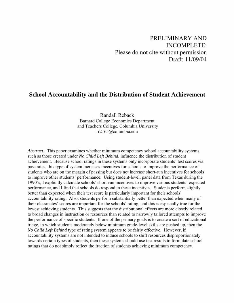
Abstract: This paper examines whether minimum competency school accountability systems, such as those created under No Child Left Behind, influence the distribution of student achievement. Because school ratings in these systems only incorporate students’ test scores via pass rates, this type of system increases incentives for schools to improve the performance of students who are on the margin of passing but does not increase short-run incentives for schools to improve other students’ performance. Using student-level, panel data from Texas during the 1990’s, I explicitly calculate schools’ short-run incentives to improve various students’ expected performance, and I find that schools do respond to these incentives. Students perform slightly better than expected when their test score is particularly important for their schools’ accountability rating. Also, students perform substantially better than expected when many of their classmates’ scores are important for the schools’ rating, and this is especially true for the lowest achieving students. This suggests that the distributional effects are more closely related to broad changes in instruction or resources than related to narrowly tailored attempts to improve the performance of specific students. If one of the primary goals is to create a sort of educational triage, in which students moderately below minimum grade-level skills are pushed up, then the No Child Left Behind type of rating system appears to be fairly effective. However, if accountability systems are not intended to induce schools to shift resources disproportionately towards certain types of students, then these systems should use test results to formulate school ratings that do not simply reflect the fraction of students achieving minimum competency.

“Under the [No Child Left Behind] law, schools must test students annually in reading and math from third grade to eighth grade, and once in high school. Schools receiving federal antipoverty money must show that more students each year are passing standardized tests or face expensive and progressively more severe consequences. As long as students pass the exams, the federal law offers no rewards for raising the scores of high achievers, or punishment if their progress lags.” (Schemo, New York Times, A1, March 2, 2004).

1. Introduction

On January 8, 2002, President George W. Bush signed into law the “No Child Left

Behind Act of 2001,” a reauthorization of the Elementary and Secondary Education Act. The

most prominent policy change instituted by the new law was to require that states adopt school

accountability systems based on minimum competency testing. The law authorizes the U.S.

Department of Education to withhold federal funds if a state does not administer a testing and

accountability system meeting several requirements. Similar to Texas’ current accountability

system, (which began when President George W. Bush was Governor), No Child Left Behind

requires states to rate schools based on the fraction of students demonstrating “proficiency.”

The focus of this paper is to examine whether accountability systems that use test score

measures based only on minimum competency influence the distribution of student achievement.

Since school ratings in these systems only incorporate test results via pass rates, this type of

system increases incentives for schools to improve the performance of students who are on the

margin of meeting these standards, while offering no incentives for schools to improve other

students’ performance. Schools might therefore concentrate on the marginal students, to the

detriment of very low achieving students and of high achieving students. Though increasing the

fraction of students meeting a minimum standard is a laudable goal, it may not be worth

lowering the quality of educational services offered to other students. Under No Child Left

Behind, schools have fairly strong incentives to focus on the pass rates, since the school ratings

1

could lead to organizational interventions,1 changes in school prestige, students transferring to

other public schools, changes in local property values,2 and financial rewards to schools and

teachers.3

In order to investigate the effect of a minimum competency accountability system on the

distribution of achievement, I analyze individual-level test score data and school-level

accountability data from Texas between 1994 and 1998.4 I exploit discontinuities created by the

passing test score and by discrete cutoffs for multiple accountability indicators such as

attendance rates, dropout rates, and the pass rates of different ethnic groups within the school.

Given that these discrete cutoffs exist, I am able to estimate the marginal effect of a hypothetical

improvement in the expected performance of a particular student on the probability that a school

obtains a certain rating. I then directly test whether students earn higher than expected test

scores when schools have stronger incentives to focus on these students’ performance. Schools

have the greatest incentives to improve the achievement of students who are on the margin in

terms of passing the exam, especially if these students fall into an ethnic subgroup with a low

passing rate.

Preliminary results suggest that schools respond to the accountability system by taking

actions which influence the distribution of student achievement. These actions appear to be

broad measures that would help low-achieving students rather than more targeted measures to 1 As of 2002, thirty-eight states had policies for sanctioning schools and/or school districts based on unsatisfactory student performance. In thirty of these states, possible sanctions included taking over a school or school district, closing a school, or re-organizing a school district (Education Commission of the States, 2002). 2 Figlio & Lucas (forthcoming) find that house prices increase in Florida when the local elementary schools receive an “A” rather than a “B” grade, even when controlling for the linear effects of the test measures used to determine the ratings. 3 In 2002, nineteen states had programs granting monetary awards to either districts or schools based on student performance. Thirteen of these states permitted the awards to go directly to teachers or principals as salary bonuses (Education Commission of the States, 2002). 4 Although data is also available for 1999 and 2000, including these years is problematic. For the first time in 1999, students taking a Spanish version of the tests contributed to the accountability ratings. Unfortunately, it is not possible to determine how these students would have scored in 1998 or whether students took the Spanish or English versions of the test in 1999 and 2000.

2

assist only the students closest to the margin for passing the exam. Within the same school

during the same year, students whose performance could most influence their school’s rating

make better improvements than other students. However, these effects are very small. Much

more educationally significant distributional effects occur when the performance of a student’s

classmates will strongly influence that school’s rating. When a school has a greater short-run

incentive to raise a pass rate, then the performance of low-achieving students increases, even if

these students have a negligible chance of passing. Schools’ short-run incentives do not cause

the performance of higher achieving students to increase by as much. These results may actually

understate the distributional effects, because schools may make permanent changes to raise pass

rates regardless of short-run incentives. Further analyses also suggest that the main results may

understate the relative gains made by students with moderate chances of passing their exam,

because schools strategically exempt the lowest performing students from test-taking and

strategically hold students back in the same grade.

In terms of education policy, the key finding is that schools somehow alter the

educational progress of students in response to the short-run incentives created by school ratings

systems. If one of the primary goals is to create a sort of educational triage, in which students

below minimum grade-level skills are pushed up, then the No Child Left Behind type of rating

system appears to be fairly effective. However, if accountability systems are not intended to

induce schools to shift resources disproportionately towards certain types of students, then these

systems should use test results to formulate school ratings that do not simply reflect the fraction

of students achieving minimum competency.

3

2. Related Literature

Recent studies explicitly examining the distributional consequences of school ratings

based on minimum competency standards focus on either relative pass rate trends over time or

the relative performance of students at various points of the distribution. Deere and Strayer

(2001) find that the passing rate on tests in Texas included in the school rating system, (8th grade

tests in reading, math, and writing), increased at a higher rate than for Texas tests not used to

determine school ratings (8th grade tests in social studies and science). They also find that

students previously scoring near or below the passing score average a larger gain in scores than

students previously scoring above the passing score. Examining student test scores in North

Carolina, Holmes (2003) cleverly uses a nonlinear model to examine test score gains for students

expected to score moderately below or moderately above the required cutoff. Assuming a null

hypothesis of symmetry in the likelihood of percentile gains with respect to a score close to the

required cutoff, he finds that students make greater gains in reading when their previous test

score was moderately below the cutoff. Unlike these studies, the empirical methodology in this

paper produces results that are robust to varying difficulty of test score gains at different points

in the test score distribution.

Another potential way to test for distributional consequences of minimum competency

school accountability systems would be to examine changes in the distribution of performance

on external assessment measures before and after the adoption of the accountability system. One

should interpret these analyses cautiously, since assessment measures will differ in their validity

and their relevance for assessing skills at various points of the ability distribution. Since the

adoption of Texas’ current accountability system in 1993, there have been large increases in

scores and pass rates on the Texas Assessment of Academic Skills (TAAS), the exam used for

4

the rating system. Figure 1 shows how the TAAS pass rates have increased over time. In order

to test the validity of these apparent achievement gains, a few recent studies examine how other

performance measures have changed in Texas over the same period. On the one hand, Texas

students have made strong gains on NAEP tests, a national test given to a random sample of

students. Grissmer & Flanagan (1998) report that, after Texas adopted its rating system, average

math NAEP scores improved in Texas considerably more than in other states, while average

reading NAEP scores kept pace with national improvements. Hanushek & Raymond (2003)

report that, for the cohort of students who were tested in 4th grade during 1996 and in 8th grade in

2000, mean student math scores on the NAEP tests increased by 0.9% more in states with

accountability programs than in states possessing neither an accountability program or a school

report card system. On the other hand, Carnoy, Loeb, and Smith (2002) present school-level

analysis suggesting that scores on the TAAS exit exams, which students initially take during 10th

grade, are not closely correlated with other educational attainment and performance measures:

(1) the fraction of 10th graders reaching 12th grade two years later, (2) the proportion of

SAT/ACT takers, or (3) the average SAT score.5

These overall findings for external outcomes are actually consistent with the hypothesis

that marginal students’ performance improves by a greater amount than very high or very low

achieving students’ performance. A plausible explanation that reconciles all of these findings is

that schools have been raising the achievement of students who are marginal in terms of passing

the TAAS, and these types of students remain likely to graduate high school on schedule but

5 Haney (2000) finds a rise in retention rates, especially for minority students, and a rise in dropout rates, though Carnoy, Loeb, & Smith (2002) argue that these trends existed prior to the adoption of TAAS so that one cannot draw causal inferences. In addition, Haney (2000) cites a rise in the fraction of students taking TAAS classified as special education (and therefore not contributing to pass rates), but Cullen & Reback (2002) explain that there was an equally large decrease in the frequency of other types of exemptions such as the fraction of students classified as special education and not even taking the TAAS.

5

unlikely to go to college. As of 1998, the statewide pass rates within ethnic groups remained

lower than the fraction of students in these groups who attended college, while the failure rates

remained higher than the fraction of students dropping out of high school. The disproportionate

gains in math scores, compared to reading scores, are also consistent with the incentives created

by Texas’ accountability system. As discussed further below, TAAS math pass rates are usually

lower than TAAS reading and TAAS writing pass rates, so that Texas’ school rating system

provides stronger incentives to raise math performance than reading performance.

Jacob (2002), using test score data from Chicago, also compares students’ relative

performance on high stakes exams and external assessments after the imposition of

accountability. In Chicago, there was both student accountability and school accountability:

students were required to achieve at roughly the 20th percentile nationally in reading and math in

order to gain promotion to certain grade levels and schools were placed on probation if less than

15 percent of students scored below the 50th percentile nationally in reading. In terms of relative

achievement gains, Jacob compares performance on the high stakes exams for students and

schools that are either on the margin or not on the margin for accountability consequences.

Consistent with the importance of school accountability, students at schools at risk of probation

made higher gains than students with similar previous scores at other schools. As for student

accountability, although students at risk of grade repetition made higher gains than in reading,

this was not necessarily true for math scores.6 Furthermore, students in the relevant grades

6 As far as overall achievement trends, Jacob (2002) finds that after these accountability measures were adopted: (1) high stakes test scores improved compared to previous performance on the same types of tests, and (2) high stakes test scores in Chicago improved compared to other Midwest cities. However, when he includes district-specific trends and control variables, he finds that performance on low-stakes exams in Chicago did not increase and in some cases decreased relative to other Illinois cities. He keenly observes that much of the apparent gains in reading achievement on the high stakes exam appear to be driven by extra student effort while taking the tests. In particular, the reading achievement gains can be almost entirely explained by increased performance on the final 20 percent of the exam questions, possibly due to students making a dedicated effort to finish the exam and to guess rather than leave questions blank, (since there was no penalty for incorrect answers).

6

where forced retention may occur did not outperform students in other grades. Although Jacob’s

findings are relevant to much of the analysis presented below, there are two key differences

between the studies. First, this paper examines the distribution of student achievement gains

across otherwise similar schools in which one school has short-run accountability incentives,

whereas Jacob’s study compares relative performance at low achieving and high achieving

schools in response to accountability. Second, in Texas there is only one margin of importance

for students’ test scores (the passing score cutoff), whereas in Chicago there were the two

margins described above.

There is also evidence of distributional effects caused by some other types of educational

accountability systems.7 Jacobson (1993) uses panel data to examine the distributional

consequences of a state requiring students to pass a minimum competency exam in order to

graduate from high school. He finds that the presence of a minimum competency graduation

requirement affects the distribution of student performance on mathematics and arithmetic tests,

but not reading tests. In particular, in states with this mandatory testing requirement, students

predicted to perform in the bottom sixth of the ability distribution performed better than expected

in mathematics, while students predicted to be in the top third performed worse than expected.

Though this mandatory testing graduation requirement places accountability directly on students

rather than on schools, this evidence suggests that schools who care about the fraction of students

7 There is little evidence on distributional effects caused by educational performance contracts, probably because these arrangements have been rare. Gramlich and Koshel (1975) analyze the test results of students in control and treatment groups of a 1971 Office of Economic Opportunity experiment that gave private contractors incentives to raise student achievement. The contractors only received revenues for each student if the student gained one year grade level equivalent, and could receive some additional revenues over a specified range of achievement gains exceeding one grade level. The authors did not find any difference in the variance of performance between students in the control and treatment groups. However, the lack of distributional effects in this case may reflect the structure of the performance contracts: since the marginal benefit from a student gaining a full year’s grade equivalency was much larger than the marginal benefit from a student making additional gains, it is unclear whether the companies should have focused on the lowest or highest performing students. Even small increases in the likelihood of a student making the full year’s progress could imply that the company should not ignore the lowest achievers.

7

meeting minimum standards may shift attention to students on the margin for meeting these

standards. This phenomenon may also be relevant in Texas, since this is one of the states that

requires students to pass exams in order to graduate high school.

Finally, there is evidence that schools engage in various other types of strategic behavior

in order to improve their accountability ratings. Hanushek & Raymond (2002) summarize the

evidence on these strategic responses. The types of behaviors include classifying students as

special education or limited English proficient in order to exempt them from testing (Figlio &

Getzler, 2002; Cullen & Reback, 2002), improving the nutritional content of school meals

shortly before the test administration (Figlio & Winicki, forthcoming), and altering disciplinary

practices (Figlio, 2003). Section 6 below examines how strategic exemptions from testing and

grade-level retention of students appear to influence this paper’s main results. The evidence

suggests that these strategic behaviors cause the findings below to understate the distributional

impact in terms of relative gains of marginal students and to overstate the impact in terms of the

gains made by the lowest performing students as a result of their school having strong incentives

to raise the test scores of their classmates.

3. Background

3.1 Texas Accountability Program

Prior to No Child Left Behind, thirty-five states used student test scores to determine

school ratings or school accreditation status. Fourteen of these states used student performance

measures to assign discrete grades or ratings to all schools and/or school districts.8 Texas’

accountability program is arguably the most well-known of these fourteen programs. It is also

8 These statistics are based on the individual state summaries compiled by the Consortium for Policy Research in Education (2000).

8

the oldest school rating system, in terms of retaining its original form and goals. As mentioned

above, the basic requirements for states’ accountability systems under No Child Left Behind are a

close fit with Texas’ current system. Since 1993, the Texas accountability system has been

annually classifying schools (and districts) into four categories. The categories are: Exemplary,

Recognized, Acceptable (Academically Acceptable), and Low-performing (Academically

Unacceptable). Which category a school falls into depends on the fraction of all students who

pass Spring achievement exams in Reading, Math, and Writing. All students and separate

student subgroups, (African American, Hispanic, White, and Economically Disadvantaged),

must demonstrate pass rates that exceed year-specific standards for each category. Pass rate

requirements for the student subgroups must be met if the subgroup is sufficiently large, meaning

either at least 200 students or at least 30 students who compose at least 10 percent of all

accountable test-takers in that subject. In addition, schools must have maintained dropout rates

less than a certain level and attendance rates above a certain level in the prior year. The year-

specific standards from 1993 to 1998 are displayed in Table 1. For some years and certain rating

levels, the rating also depends on the amount of improvement in the campus’ pass rate from the

previous year.

The Texas Education Agency also publishes how schools’ mean student one-year test

gains rank against a group of comparison schools.9 Although this variable does not affect a

school’s accountability rating, this type of reporting may mitigate the incentives to focus only on

9 Since 1995-96, the TEA annually assigns each school a unique comparison group of forty based on similar demographic characteristics: the percentages of students who are Black, Hispanic, White, limited English proficient, economically disadvantaged, and mobile (i.e., did not attend the same school in the Fall and Spring). The TEA then acknowledges some schools that make strong progress in either reading or math test score growth relative to their comparison groups. These “comparable improvement” acknowledgements are completely independent from the main accountability ratings. They are not based on changes in pass rates, but rather on: (1) relative comparisons of the average score increase for students scoring less than a 85 (out of 100) on the Texas Learning Index during the previous year and (2) the fraction of students who score a 85 or higher during the previous year. For example, in 1998, a school was acknowledged if the mean score increase was in the top quartile of its comparison group and at least 50% of students with scores available from the prior year scored 85 or higher.

9

marginal students. The distributional consequences of a pass rate accountability system would

likely be even more severe if, unlike Texas, a state did not report other performance indicators.

3.2 Theoretical Framework for “Teaching to the Rating”

In order to provide some insight concerning how schools would react to a minimum

proficiency accountability system, this section presents a model based on behavior under a

simplified version of this type of system. Consider a system in which the only indicators used to

determine the ratings are the campus-wide pass rates on reading and math tests. To simplify the

analysis, the theoretical framework below uses two non-essential assumptions. First, assume that

resources can only be transferred within classrooms. If school administrators may also

strategically transfer resources across classrooms, then one could model analogous shifts that

would further magnify changes in the distribution of student achievement gains. Second, assume

that administrators and teachers are concerned only with student achievement for the current

year. In reality, they are likely treating this as a dynamic problem, in which achievement gains

that do not help the school’s rating this year but would likely help in the future are still valuable.

By assuming this is a one-period optimization problem, this analysis underestimates the

incentive to improve the achievement of low-performing students, particularly those in the lower

grades who may be closer to a passing score by the time they enter high school. Though I ignore

this here, some of the empirical analyses in future drafts will address this issue by testing for

differential effects across grade levels.

Suppose that the total level of resources within a classroom is fixed. One may aggregate

all of the potential classroom resources: teacher time, teacher effort, books, other instructional

materials, etc. into three general types of inputs. One type of input is subject-specific and serves

10

all students, such as spending time on a Math lesson that equally helps all students learn. A

second type of input is subject-specific and student-specific, such as individually helping a

particular student with Math. The third type of input is student-specific and serves all subjects,

such as giving individual attention to a student’s study-skills or behavior. Let as denote

resources devoted to helping all students with subject s, let bi denote a resource dedicated to

student i that is not subject-specific, and let cis a resource devoted to helping student i with

subject s.

In the absence of the ratings system, teachers have prior attitudes about the relative

importance of helping students improve in certain subjects and the relative importance of helping

different types of students make improvements. Suppose that subjects fall into three categories:

Reading (denoted by s=r), Math (s=m), and all other subjects (s=z). Teachers in a classroom

with N students and total resources equal to T will choose ar, am, az, bi, cir, cim, and ciz [ ]N,1i ∈∀ to

maximize:

(1A) , ∑∑∑===

++N

iiziziziz

N

iimimimim

N

iiriririr cbafcbafcbaf

111),,(),,(),,( γγγ

with , 1)( =++∑N

iizimir γγγ

subject to:

(1B) , for some constant T>0 ∑=

=++++N

iisizmr Tcbaaa

1 )(

with 0,0,0 >∂∂

>∂∂

>∂∂

is

is

i

is

s

is

cf

bf

af

, N][1,i ∈∀{ }zm,r,s ∈∀ .

11

In equation (1A), fir(.), fim(.), fiz(.) denote the achievement of student i in reading, math, and other

subjects respectively, which will be a function of the student-specific general resources (bi), the

student-subject-specific resources (cis for subject s), and the whole-class subject-specific

resources (ar for reading, am for Math, az for other). The weights, γir, γim, and γiz, are used to

represent the teacher’s own valuations of the relative importance of the performance of student i

in reading, math, and other subjects respectively.

Now suppose an accountability/testing system is introduced. One concern is that teachers

will begin “teaching to the test.” Shifting resources in order to try to raise students’ test scores is

not inherently a bad thing. However, the phrase “teaching to the test” usually implies an

undesired type of behavior modification in which a more valuable type of instruction is

sacrificed. Teaching to the test could be harmful if the tests do not cover a sufficiently wide

range of subjects or if the teachers devote resources in a way intended to improve students’ test

performance without creating any real achievement gains, improvements that other types of

assessments would also measure.

The focus of this paper is not on “teaching to the test,” but more generally on “teaching to

the rating.” “Teaching to the rating” occurs when teachers have incentives to maximize the

rating awarded to their school. In the extreme case, a teacher will completely abandon the

previous objective function (equation 1A) in favor of one that maximizes the school’s rating.

This will be done by maximizing some function related to the reading and math pass rates in the

teacher’s own classroom:

Choose ar, am, az, bi, cir, cim, and ciz [ ]N,1i ∈∀ to maximize:

(2) ⎟⎟⎠

⎞⎜⎜⎝

⎛≥⎟

⎠

⎞⎜⎝

⎛⎟⎟⎠

⎞⎜⎜⎝

⎛≥⎟

⎠

⎞⎜⎝

⎛= ∑∑

==

TcbafPTcbafPvN

iimimimim

N

iiriririr

~)),,((Prob*~),,((Prob)c,c ,c ,b ,a ,a ,a(11

izimirizmr

12

Subject to equation (1B)

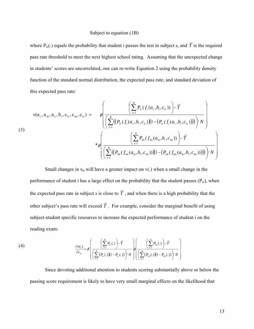
where Pis(.) equals the probability that student i passes the test in subject s, and T~ is the required

pass rate threshold to meet the next highest school rating. Assuming that the unexpected change

in students’ scores are uncorrelated, one can re-write Equation 2 using the probability density

function of the standard normal distribution, the expected pass rate, and standard deviation of

this expected pass rate:

(3) ( ) ( )( )( )

( ) ( )( )( ) ⎟⎟⎟⎟⎟

⎠

⎞

⎜⎜⎜⎜⎜

⎝

⎛

⎟⎠

⎞⎜⎝

⎛−

−⎟⎠

⎞⎜⎝

⎛

⎟⎟⎟⎟⎟

⎠

⎞

⎜⎜⎜⎜⎜

⎝

⎛

⎟⎠

⎞⎜⎝

⎛−

−⎟⎠

⎞⎜⎝

⎛

=

∑

∑

∑

∑

=

=

=

=

NcbafPcbafP

TcbafP

NcbafPcbafP

TcbafPv

N

iimimimimimimimim

N

iimimimim

N

iiririiriririir

N

iiririir

/)),,((1)),,((

~)),,((*

/),,((1),,((

~)),,(( )c,c ,c ,b ,a ,a ,a(

1

1

1

1izimirizmr

φ

φ

Small changes in xis will have a greater impact on v(.) when a small change in the

performance of student i has a large effect on the probability that the student passes (Pis), when

the expected pass rate in subject s is close to T~ , and when there is a high probability that the

other subject’s pass rate will exceed T~ . For example, consider the marginal benefit of using

subject-student specific resources to increase the expected performance of student i on the

reading exam:

(4)

( )( ) ( )( ) ⎟⎟⎟⎟⎟

⎠

⎞

⎜⎜⎜⎜⎜

⎝

⎛

⎟⎠

⎞⎜⎝

⎛−

−⎟⎠

⎞⎜⎝

⎛

⎟⎟⎟⎟⎟

⎠

⎞

⎜⎜⎜⎜⎜

⎝

⎛

⎟⎠

⎞⎜⎝

⎛−

−⎟⎠

⎞⎜⎝

⎛

′=∂∂

∑

∑

∑

∑

=

=

=

=

NPP

TP

NPP

TP

cv

N

iimim

N

iim

N

iirir

N

iir

ir /(.)1(.)

~(.)

/(.)1(.)

~(.)(.)

1

1

1

1 φφ

Since devoting additional attention to students scoring substantially above or below the

passing score requirement is likely to have very small marginal effects on the likelihood that

13

these students pass (Pis), one would predict a shift of resources away from these students and

towards students marginally close to earning a passing score.

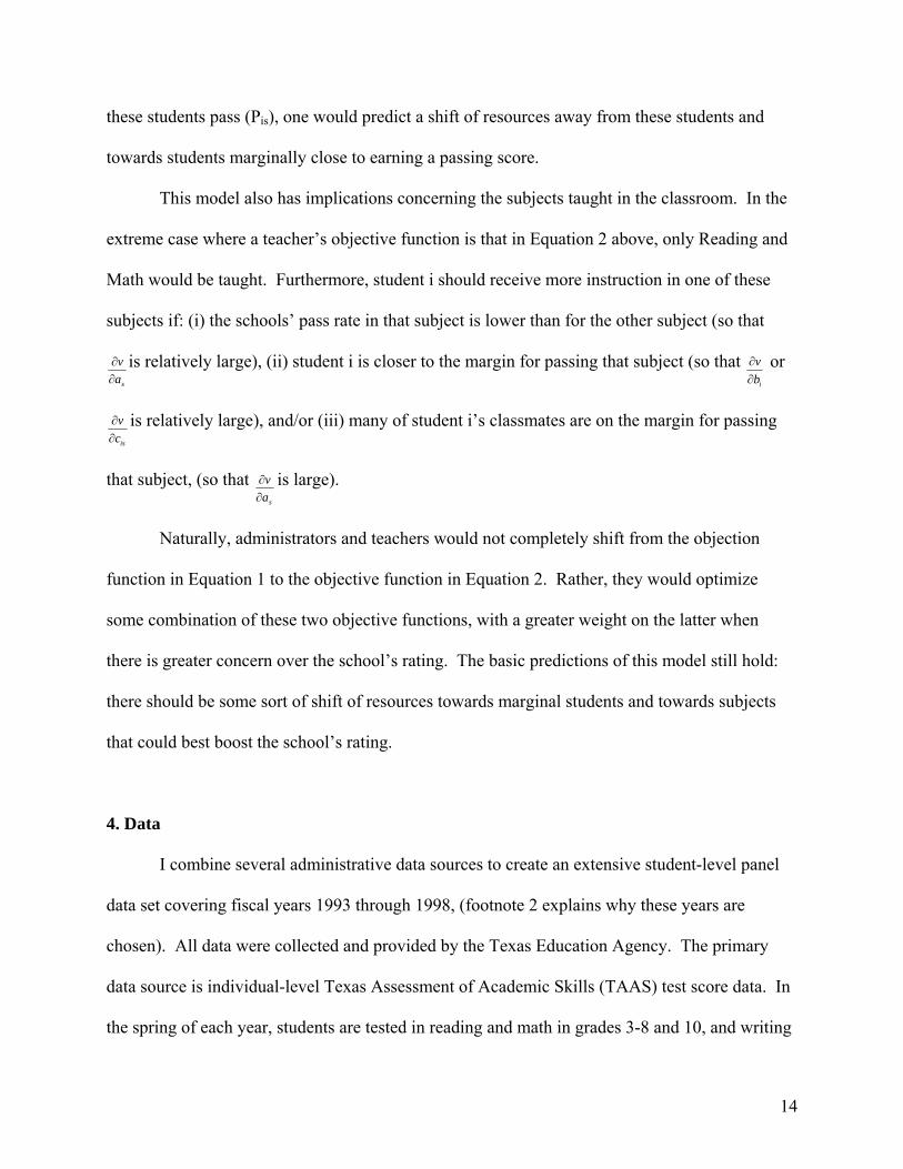
This model also has implications concerning the subjects taught in the classroom. In the

extreme case where a teacher’s objective function is that in Equation 2 above, only Reading and

Math would be taught. Furthermore, student i should receive more instruction in one of these

subjects if: (i) the schools’ pass rate in that subject is lower than for the other subject (so that

sav

∂∂ is relatively large), (ii) student i is closer to the margin for passing that subject (so that

ibv

∂∂ or

iscv

∂∂ is relatively large), and/or (iii) many of student i’s classmates are on the margin for passing

that subject, (so that sa

v∂∂ is large).

Naturally, administrators and teachers would not completely shift from the objection

function in Equation 1 to the objective function in Equation 2. Rather, they would optimize

some combination of these two objective functions, with a greater weight on the latter when

there is greater concern over the school’s rating. The basic predictions of this model still hold:

there should be some sort of shift of resources towards marginal students and towards subjects

that could best boost the school’s rating.

4. Data

I combine several administrative data sources to create an extensive student-level panel

data set covering fiscal years 1993 through 1998, (footnote 2 explains why these years are

chosen). All data were collected and provided by the Texas Education Agency. The primary

data source is individual-level Texas Assessment of Academic Skills (TAAS) test score data. In

the spring of each year, students are tested in reading and math in grades 3-8 and 10, and writing

14

in grades 4, 8, and 10. Each school submits test documents for all students enrolled in every

tested grade. This means that students that are exempted from taking the exams due to special

education and limited English proficiency (LEP) status are included. The test score files,

therefore, capture the universe of students in the tested grades in each year. In addition to test

scores, the data include the student's school, grade, race/ethnicity, and indicators of economic

disadvantage, migrant status, special education, and limited English proficiency. The data do not

include the student's gender.

The Texas Education Agency provided versions of these data that assign each student a

unique identification number. This number is used to track the same student across years, as

long as the student attends any Texas public school.10 I combine this student-level, test score

data with campus-level data used by the Texas Education Agency that contains information used

to determine school accountability ratings: the size of racial/economically disadvantaged

subgroups, attendance rates, and dropout rates. In addition, the data contain other campus-level

information, such as the total number of students enrolled in various grades.

The specific test outcomes are Texas Learning Index (TLI) scores based on the TAAS

exam. The TLI is intended to measure how a student is performing compared to grade level. A

score of 70 or greater is considered a passing score, meeting expected grade-level proficiency.

The difference in a student’s T.L.I. scores from one year to the next is intended to capture

whether this student remains in the same place compared to grade-level, so that a student scoring

10 In practice, there appears to be a low frequency of coding errors in the data, as discussed by Hanushek, Kain, & Rivkin (2004) who use a similar data set. 1.7% of the TEA data are composed of observations that have identification numbers which are identical to the identification numbers of other observations in the same year. However, I am able to keep over 81% of these duplicate cases in the sample, by identifying which identification number corresponds with identification numbers from other years, based on information concerning the students’ race, grade, and school district. As in other studies, there is likely a limited amount of sample attrition due to incorrect identification numbers for students who remain in the Texas public school system for consecutive years, but whose identification numbers are not linked across the years due to the erroneous identification numbers.

15

72 in 4th grade and 76 in 5th grade is more advanced in 5th grade in terms of both an absolute and

relative to grade-standard sense.

In this paper, certain types of student-level observations are used to estimate the school’s

accountability incentives but are not included in the actual regression analyses. Observations

with prior year’s TLI scores below 30 or above 84 are removed from the regression analyses,

because there is less room for these students to decrease or increase respectively since the scores

are capped at 20 and 100.11 The Texas Education Agency similarly restricts the sample when

formulating comparisons of schools’ mean one-year test score gains.12

Other sample restrictions in the regression analyses include dropping students whose tests

were not scored during either the current year or the previous year because the score did not

contribute to the accountability ratings due to an exemption. Cullen & Reback (2002) describe

exemption practices in Texas over this sample period. The reasons for this type of exemption

include the student was severely disabled and thus unable to take the test, the student was limited

English proficient (LEP), the student was absent during the testing, or some “other” reason such

as an illness during the testing. In addition, students are dropped from the regression analyses if

they were designated as “mobile,” meaning that their scores do not contribute to the schools’

accountability ratings because they did not attend the same public school district earlier in the

school year. Finally, students are dropped from the regression analyses if they are classified as

receiving special education and thus do not contribute to the ratings, even if they were able to

take the test. As discussed below, schools’ strategic behavior in terms of exempting students

11 I impose a score of 20 as the minimum score, because, although slightly lower scores occasionally occur in the data, they are likely the result of blank exam sheets for observations in which the scoring code variable was incorrectly marked “scored.” 12 Aside from the school accountability ratings, the TEA (Texas Education Agency) makes less-publicized acknowledgements in which they rank schools’ mean one-year test gains relative to comparison schools (see footnote 9). TEA does not use the one year changes in a students score if the previous year’s score was 85 or higher, arguing that these one year changes are not informative when the scores are near the maximum score (100).

16

would generally cause this paper’s main findings to understate the distributional effects on

student achievement.

The remaining sample used for the regression analyses consists of 1,450,480 observations

for Reading score gains and 1,977,633 observations for Math score gains. The larger sample size

for Math scores is mostly due to a much larger percentage of Reading TLI scores that are too

high to reveal meaningful gains (scores of 85 or higher).13

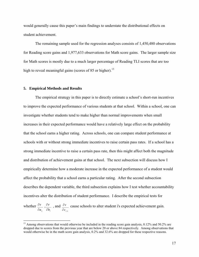
5. Empirical Methods and Results

The empirical strategy in this paper is to directly estimate a school’s short-run incentives

to improve the expected performance of various students at that school. Within a school, one can

investigate whether students tend to make higher than normal improvements when small

increases in their expected performance would have a relatively large effect on the probability

that the school earns a higher rating. Across schools, one can compare student performance at

schools with or without strong immediate incentives to raise certain pass rates. If a school has a

strong immediate incentive to raise a certain pass rate, then this might affect both the magnitude

and distribution of achievement gains at that school. The next subsection will discuss how I

empirically determine how a moderate increase in the expected performance of a student would

affect the probability that a school earns a particular rating. After the second subsection

describes the dependent variable, the third subsection explains how I test whether accountability

incentives alter the distribution of student performance. I describe the empirical tests for

whether sa

v∂

∂ , ib

v∂

∂ , and ,sic

v∂

∂ cause schools to alter student i's expected achievement gain.

13 Among observations that would otherwise be included in the reading score gain analysis, 0.12% and 50.2% are dropped due to scores from the previous year that are below 20 or above 84 respectively. Among observations that would otherwise be in the math score gain analysis, 0.2% and 32.6% are dropped for these respective reasons.

17

5.1 Estimating the Marginal Benefit to the School from a Moderate Increase in a Student’s

Expected Performance

In order to conduct the empirical analysis, I first estimate the marginal benefit to the

school from a moderate increase in a student’s expected performance. This involves calculating

a partial derivative similar to ,sic

v∂

∂ from Equation 4, the marginal change in the probability that a

school earns a higher rating due to a change in the level of a student-specific resources. There

are three steps involved with calculating this partial derivative.

First, I estimate the probability that each student passes by grouping students based on

their performance during other years. The pass probability equals the mean pass rate within

these groups. For grades 4 though 8, groups are based on students with identical scores in

Reading or identical scores in Math during the prior year, depending on which subject is the

outcome of interest. If students are missing prior year scores for certain subjects, I use the other

subject score if available, or else use scores from the following year.14 For grade 10, since

students are not tested in grade 9, the groups are based on students with identical scores in grade

8 (two years earlier). For all grades, any remaining missing values for student-level pass

probabilities are assigned the mean estimated pass probability for students that year in the same

grade at the same school. For grade 3, since this is the first grade of testing and prior scores are

never available, I assign the same pass probability to all students within a school, based on the

14 Although scores from the following year are positively related to shocks in current year scores, there is not an endogeneity problem in this context, because these predicted scores are used simply to determine the expected school-level pass rates. The student-level regression analyses only include students whose scores are predicted based on prior scores and not future scores.

18

scores of the previous year’s cohort within that school.15 School administrators and teachers

likely expect an achievement distribution similar to that of the previous year’s third grade cohort,

adjusted for upward trends in achievement.

Second, I use these student-level pass probabilities to compute the probability that the

school will obtain each rating, based on a version of Equation 3 that includes all performance

indicators. This analysis only includes pass probabilities for students whose actual scores

contributed to schools’ pass rates for the accountability system. The probability that a school

makes a certain rating equals the product of the probabilities that the pass rates (both campus-

wide and within student subgroups), attendance rate, and dropout rates for this school each meet

the relevant requirement.16

Finally, I find the marginal effect of a moderate improvement in the expected

achievement of a particular student on the probability that the school obtains the various ratings.

There is theoretical ambiguity concerning the magnitude of changes in a student’s expected

performance due to moderate changes in the amount of resources devoted to that student. My

preferred approach is to increase expected student performance in a way that is related to the

actual distribution of achievement for similarly skilled students. In particular, I calculate a new,

hypothetical pass probability by re-estimating the student’s pass probability after dropping the

bottom X% of the current year score distribution within the previously established predicted pass

rate groups. In the analyses below, X is set to 50, so that the hypothetical improvement is as if

15 Rather than simply using the prior cohort’s pass rate, I adjust the pass probability for upward trends in performance. I find the statewide percentile of third grade students who passed in year t, and then calculate the fraction of students in each school’s third grade that scored at that percentile or better in year t-1. 16 This assumes that unexplained students performance is not correlated across students within a school. In reality, unexplained performance is likely positively correlated within schools, because there may be common shocks like distracting noise on the test day or a better than usual teacher that year. In this case, the estimated probabilities that a school achieves a rating will understate the actual probability for schools that have low probabilities and overstate the probability for schools that have high probabilities. If anything, this would likely cause this paper’s empirical analyses to underestimate distributional effects, because the estimated marginal impact of improving a particular student’s performance would be less accurate.

19

the student is guaranteed not to finish in the bottom half of the distribution of students with

similar pre-existing skills. The results are qualitatively similar to those below if X=10 or X=20

or X=80. If the student’s estimated pass probability was actually p and if the Xth percentile

student with similar pre-existing skills fails the exam, then this implies a new, hypothetical pass

probability of

⎟⎠⎞

⎜⎝⎛ −

1001 X

p . If the Xth percentile student with similar pre-existing skills passes the

exam, then the new, hypothetical pass probability equals 1.

5.2 Analyzing the Distribution of Performance in a Value-added Achievement Model

Various models below regress a value-added measure of student performance on

measures that estimate the incentives for a school to improve a student’s performance, as well as

a set of campus, peer and individual-level control variables. The dependent variable is based on

one-year improvements in student-level test scores. Unlike previous studies analyzing test score

gains, this analysis adjusts for the possibility that one-year differences in test scores might

signify more or less substantial gains at different points in the test score distribution. Rather than

using the difference between the current and prior year’s scores or the difference between

monotonic transformations of those scores, I transform these gains to allow for comparability in

improvements across the entire test score distribution. In particular, I convert the current year’s

score to a Z-score based on the performance of students with identical prior year’s scores in

identical grades. Each Z-score represents the place in the standard normal distribution for the

current year’s score based on similar performance in the prior year. This standardization allows

one to compare students with different achievement levels in a more meaningful fashion. One

may interpret a coefficient estimate as how the independent variable relates to achievement gains

20

compared to typical gains at this place in the test score distribution.17 The results will thus not

be influenced by mean reversion or other factors unrelated to school incentives which would

make test score gains more difficult at various points in the performance distribution.

Define TLI_MATH as the mathematics Texas Learning Index score and TLI_READ as

the reading Texas Learning Index score. For student i enrolled in grade g during year t, the

dependent variable, Yi,g,t equals the standardized test score gain:

(5) [ ]

21,1,,,1,1,

2,,

1,1,,,,,,,

]_|_[]_|_[

_|__

−−−−

−−

−

−=

tgitgitgitgi

tgitgitgitgi

MATHTLIMATHTLIEMATHTLIMATHTLIE

MATHTLIMATHTLIEMATHTLIY ,

when Math test scores are used. (An analogous dependent variable is used to analyze Reading

test performance.)

5.3 Incorporating Accountability Incentives into the Achievement Models

One would not want to simply regress student achievement measures on the estimates of

the partial derivatives described in Section 5.1. Several issues arise related to the theoretical

framework presented earlier. First, schools will vary in the size of their populations.

Schools with greater student populations will inherently have smaller benefit from improving the

expected achievement of a single student. One student’s performance can only have a limited

effect on aggregate pass rates. Second, these student-level partial derivatives are calculated

holding the expected performance of all other students constant. Schools should assess the net

17 For example, suppose that observations with prior year’s TLI scores in the 60’s were, on average, 3 points higher if the student’s school had a strong incentive to improve the pass rate. Suppose further that observations with prior year’s TLI scores in the 40’s were 3 points higher if the student’s school had a strong incentive to improve the pass rate. One might erroneously conclude that the presence of school incentives had similar effects on achievement across the test score distribution. A 3 point increase in the 60’s might represent a much larger deviation from typical gains than a 3 point increase in the 40’s, so that schools with strong incentives to improve pass rates are dramatically improving the performance of students who had scored in the 60’s but only slightly increasing the performance of students who had scored in the 40’s.

21

benefit from re-allocated resources for several students at a time, rather than simply assessing the

net benefit from only helping one student. The relevant decision is probably whether to attempt

to improve the performance of 5% of the student population in Math, not whether it is

worthwhile to improve the Math performance of a single student. In addition, teachers and

principals may consider using inputs that simultaneously improve expected achievement for

more than one student. Whether a student is helped or hurt by accountability incentives may

thus reflect incentives due to the composition of the students’ classmates. The regression models

below take these considerations into account.

5.3.1 Campus-year Fixed Effects

The first model uses campus-year fixed effects, so that the relevant comparison is which students

within a school during a particular year receive the largest boosts in achievement. This model is:

(6) stjittjtististjistisi

tjstgi YCSRPEERR

xv

Y ,,,5,4,3,1,2,1,,,1,,

,1,,, log εβββββ +++++⎟

⎟⎠

⎞⎜⎜⎝

⎛

∂

∂= −−− ,

where si

tj

xv

,

,

∂

∂ equals the marginal change in the probability that school s earns a higher rating in

year t, given the hypothetical improvement described earlier for student i in subject s. Using the

log of this partial derivative allows the results to be readily interpretable as a percent change in

the incentives and ensures that they are not unduly influenced by relatively large values of si

tj

xv

,

,

∂

∂.

Controlling for peer achievement levels and student characteristics will help to ensure

that β1 is not biased due to a correlation between accountability incentives and some omitted

variable. is a vector of control variables for past peer performance on the exams. In

particular, contains variables measuring the quintile mean scores at the grade-level for

1,, −tjiPEER

1,, −tjiPEER

22

the same subject as the dependent variable. The effect of peer achievement may differ

depending on a student’s own performance level. Therefore, is interacted with Ri,t-1,s,

a vector of dummy variables equal to one if student i's test score from the previous year fell in

that range. The ranges are 30-44 (lowest achieving), 45-54 (very low achieving), 55-64 (low

achieving), 65-74 (marginal), and 75-84 (proficient). These ranges are also enter the equation

separately in order to allow for varying intercepts.

1,, −tjiPEER

tiS , is a vector of control variables for student characteristics, including cubic terms for

the student’s previous test scores for the subject (Reading or Math) that is not being used for the

dependent variable. (The previous test score in the subject that is used for the dependent variable

is already incorporated into the value of the dependent variable.) The other student characteristic

control variables are dummy variables for a student’s race, a dummy variable for whether the

student comes from a “low-income” family, and interaction terms for these race and income

measures. Similar to how the TEA defines the economically disadvantaged subgroup, a student

is designated as coming from a low-income family if the student is eligible for free or reduced-

price lunches funded by federal subsidies. Table 3 lists all of the independent variables along

with their sample statistics.

Cj,t and Yt are vectors of dummy variables for the student’s campus (school) and the year

respectively, so that β5 captures campus-year fixed effects.

Table 4 displays estimation results for equation 5. Results are presented for models that

include or omit peer achievement levels. For math performance, the student-level accountability

incentives appear to have a very small, positive impact on students’ test score gains. The

estimated coefficient of β1 in the first row of the first column of Table 4 is .00090, with a

standard error of .00013. This implies that if a student has an accountability incentive that is

23

100% greater than another student at that school, then on average the former student will have a

math score gain that is .0009 standard deviations larger than the latter. Furthermore, a one

standard deviation increase in the student-level accountability incentive is associated with an

increase in the dependent variable of about .0045. Since these outcomes are in terms of one year

gains among students’ with initial scores, it may be helpful to convert this effect into a measure

more typically found in the previous literature, the number of standard deviations that a student

would gain or lose in the statewide testing distribution. An increase in the dependent variable of

.0045 translates into a gain of roughly .05 Texas Learning Index points, varying slightly

depending on the student’s place in the distribution. Since the statewide variation in the Texas

Learning Index equals about 10, a .05 increase in the Texas Learning Index is associated with

about a .005 standard deviation increase in the student’s place in the statewide distribution of test

scores. Thus, the effect size associated with a one standard deviation change in the student-level

accountability incentive within a school is a .005 standard deviation gain for that student in the

statewide test score distribution. This small effect is not very educationally significant.

Consider, for example, that the within-school difference in test score gains between white

students who are from low-income families versus white students who are not from low income

families is more than twenty-four times as large as this effect. The last row of Table 4 displays

similar effect sizes for the other campus-year fixed effect models. The effect of the student-level

accountability incentive is even smaller in magnitude for reading performance and is not

statistically different from zero. Overall, the evidence suggests that there are only minor

distributional consequences on achievement due to schools shifting student-specific resources.

24

5.3.2 Cross-sectional Estimates Using the Mean Incentive to Improve the Performance of a

Fraction of the Students

As described above, the marginal effect from changing only one student’s performance

may not accurately reflect the benefit-cost analyses that may lead schools to alter the distribution

of student achievement. In order to allow for cross-sectional comparisons of schools, this section

replaces si

tj

xv

,

,

∂

∂with an alternative variable, based on the relative ranking of this marginal

incentive measure among students within the school. First, I group students into twenty groups

within each school during each year based on their values of si

tj

xv

,

,

∂

∂. Next, I compute the change

in associated with all of the students within a group improving their performance by . In

other words, I compute the change in the probability that a school earns a higher rating when a

group of students all make improvements. This measure is thus related to whether there are high

incentives to improve several students’ achievement. While the groups are chosen based on the

marginal change due to a single student’s improvement, these groupings may closely reflect

infra-marginal incentives to improve a single student’s performance.18 An additional benefit of

this approach is that the issue of school size is implicitly accounted for by the division into

twenty percentile groups.

tjv , six ,

Rather than using campus-year fixed effects as in equations 5, these models analyze

variation across campuses and across time including campus-level control variables and year

fixed effects. Define as a vector of cubic terms for various school-level control variables: tjS ,

18 Given that the ratings system uses multiple performance indicators, there may be non-linearities in terms of the marginal benefits of helping certain students as different groups of their schoolmates receive extra attention. It would be nearly impossible to compute the maximum incentive for the school to boost the performance of each student, given that there are a myriad of possible groupings of students receiving extra help.

25

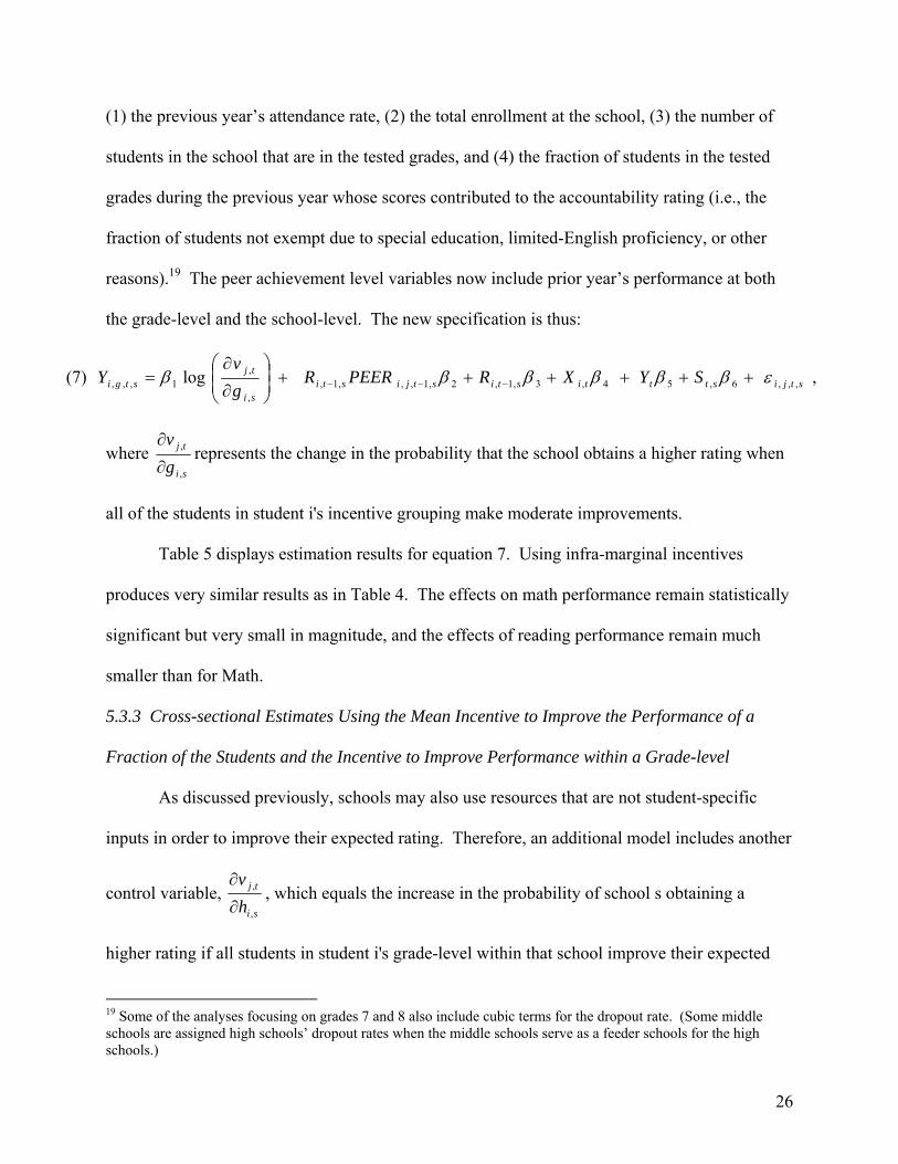
(1) the previous year’s attendance rate, (2) the total enrollment at the school, (3) the number of

students in the school that are in the tested grades, and (4) the fraction of students in the tested

grades during the previous year whose scores contributed to the accountability rating (i.e., the

fraction of students not exempt due to special education, limited-English proficiency, or other

reasons).19 The peer achievement level variables now include prior year’s performance at both

the grade-level and the school-level. The new specification is thus:

(7) stjistttististjistisi

tjstgi SYXRPEERR

gv

Y ,,,6,54,3,1,2,1,,,1,,

,1,,, log εββββββ ++++++⎟

⎟⎠

⎞⎜⎜⎝

⎛

∂

∂= −−− ,

where si

tj

gv

,

,

∂

∂represents the change in the probability that the school obtains a higher rating when

all of the students in student i's incentive grouping make moderate improvements.

Table 5 displays estimation results for equation 7. Using infra-marginal incentives

produces very similar results as in Table 4. The effects on math performance remain statistically

significant but very small in magnitude, and the effects of reading performance remain much

smaller than for Math.

5.3.3 Cross-sectional Estimates Using the Mean Incentive to Improve the Performance of a

Fraction of the Students and the Incentive to Improve Performance within a Grade-level

As discussed previously, schools may also use resources that are not student-specific

inputs in order to improve their expected rating. Therefore, an additional model includes another

control variable, si

tj

hv

,

,

∂

∂, which equals the increase in the probability of school s obtaining a

higher rating if all students in student i's grade-level within that school improve their expected

19 Some of the analyses focusing on grades 7 and 8 also include cubic terms for the dropout rate. (Some middle schools are assigned high schools’ dropout rates when the middle schools serve as a feeder schools for the high schools.)

26

performance. (I use grade-level rather than classroom-level because one cannot identify

classrooms in the data.) Given that a grade contains many students, improvements in the

expected performance of all students within a grade are unlikely to be huge. Therefore, I set X at

20 instead of 50 for the analyses described below, so that higher expected performance is only

associated with a student not scoring in the bottom 20 percent of students with similar previous

scores. As with the other models, the results are very similar regardless of the value of X.

Since altering inputs within a grade level may have differential effects on students of

different abilities, I interact si

tj

hv

,

,

∂

∂ with the previously established ranges of previous test

performance. This modified model is:

(8)

.

log

,,,7,

,,1,6,5

4,3,1,2,1,,,1,,

,1,,,

stjisi

tjstistt

tististjistisi

tjstgi

hv

RSY

XRPEERRgv

Y

εβββ

ββββ

+∂

∂+++

+++⎟⎟⎠

⎞⎜⎜⎝

⎛

∂

∂=

−

−−−

The estimation results for equation 8, presented in Table 6, reveal that there may be

important distributional effects related to the fraction of students in the grade at the school whose

performance could influence the school’s rating. Students make much higher than expected

improvements when their grade-mates may strongly influence the school’s rating. The

magnitudes of these effects are non-trivial and are generally greater for students with lower

abilities. For the lowest performing students, a one standard deviation increase in the mean

grade-level incentive leads to a .082 standard deviation increase in the statewide Math

distribution or a .010 standard deviation increase in the statewide Reading distribution.

However, for “proficient” students, those previously scoring between 75 and 84, these effects are

0.061 and 0.004 respectively. For mathematics, the gains of “proficient” and “marginal”

27

students related to their school’s grade-level incentives are smaller than for all other students at

statistically significant levels. For reading, the gains of “proficient” students are smaller than for

all other students at statistically significant levels. While all students in the sample significantly

benefit from being in a grade in which a school has a strong incentive to raise some students’

expected performance, low achievers appear to benefit at least 20% more than do marginal or

high achieving students.

Similar to Table 5, Table 6 reveals that a one standard deviation increase in the student-

level accountability incentive increases a student’s math performance by about .01 standard

deviations and has a negligible effect on a student’s reading performance. In terms of test score

improvements, whether a student’s classmates’ performance will affect the school’s rating is

much more important than whether the student’s own performance will affect this rating.

The next section will verify that these effects are truly due to changes in school services

or instructional practices rather than due to strategic exemptions of certain low performing

students from contributing to schools’ pass rates. This is particularly important because the

largest effects are for the lowest performing students, those who have extremely small

probabilities of passing.

6. Robustness Checks

6.1 The Effects of Sample Selection due to Student Exemptions and Grade Repetition

To estimate the impact of strategic exemptions and grade repetition, I repeat the analyses

above but include all students in the relevant grades and replace the dependent variable with an

indicator either for whether the student was exempted or whether the student was retained.

These types of strategic behavior influence the sample in the main analysis, though it will only

28

influence the key coefficients of interest if there is selection based on unobservable

characteristics. If anything, exempted students are likely to perform worse than observationally

equivalent non-exempted students, so that a high reported propensity to be exempted suggests

that a student who remains in the sample may be better along unobserved dimensions.

For the campus-year fixed effect model, analogous to equation 6, I find a statistically

significant, negative relationship between the student-level accountability incentive and the

likelihood that a student is exempted from the accountability pool. This suggests that the

estimated effect of the student-level accountability incentive may understate the true effect;

students with low values for the student-level accountability incentive who are not exempted

likely possess unobserved, positive characteristics in terms of their ability to perform well on the

test.

For retention within the grade, there is a small, positive relationship between the student-

level accountability incentives and the probability of grade retention. Schools that face strong

accountability incentives appear to disproportionately retain students who are low achieving or

marginal achieving but not very low achieving. This appears to be attempts to game the system:

since students’ scores contribute regardless of whether they are repeating the grade, schools

appear to be retaining some students who will likely pass the exam when retained rather than

retaining some students who may not pass the exam even if they are retained. Given the conflict

between schools’ accountability incentives and normal incentives to retain the worse students, it

is theoretically ambiguous whether these retained students are better or worse than other students

along unobserved dimensions. In any case, the effect appears to be sufficiently small that the

main distributional effects discussed in the previous section are not significantly influenced by

29

grade retention practices. In future drafts, I will also analyze retentions and exemptions in an

empirical framework similar to the other models in Section 5.

6.2 Re-estimating the results using Counterfactual Cutoff points

In future drafts, I hope to re-estimate the analyses using counterfactual cutpoints for the

required pass rates that schools must achieve to earn the various ratings. I predict that the

coefficients of the accountability incentive variables will be close to zero or will reverse their

sign. This analysis will ensure that the results are not due to some bizarre non-linear relationship

between a school being close to a pass rate cutpoint and the distribution of test score gains at that

school. Given the extensive set of control variables in the main analyses, this type of bias seems

unlikely.

7. Conclusion

The findings suggest that short-run incentives created by a minimum competency

accountability system affect the distribution of student performance gains. These distributional

effects are not strongly related to schools’ narrowly tailored attempts to improve the performance

of the students’ who are on the margin for passing or failing exams. The relative importance of a

student’s performance within a school has only a very small, positive effect on that student’s test

score gains compared to the gains of his or her schoolmates. The largest distributional effects

appear to be related to broad efforts which cause higher than expected gains among all low

performing students. When a school has a strong incentive to increase the performance of many

students in a particular grade, then low performing students in that grade at that school make

much higher than expected test score gains. Students who have previously passed the exam or

come very close to passing the exam also make higher than expected gains in this situation, but

30

they do not benefit nearly as much as other students. The largest gains compared to typical

performance are actually accomplished by students with very low probabilities of passing the

exam rather than by students with moderate probabilities of passing the exam. These results hold

when controlling for previous peer achievement levels, and the results do not appear to be

strongly affected by schools’ efforts to strategically exempt students from taking the exams.

The advantage of the estimates in this paper, which are based on comparisons with

typical achievement gains made at each point in the achievement distribution, is that they are

unaffected by variation in the difficulty of exams across time or across different parts of the

achievement distribution. They are also based directly on the short-run incentives faced by

schools. These estimates may in fact understate the distributional consequences of the minimum

competency accountability system, because schools might concentrate on low performing or

marginally performing students after the adoption of the accountability system in a permanent

fashion, rather than waiting for years in which the incentives are greatest. In addition, it is

possible that accountability incentives negatively affect the performance of the numerous

students whose scores are so high that their performance on the TAAS is not an accurate measure

of their academic progress. Since the TAAS is inherently a minimum skills test, a school’s focus

on basic skills may cause proficient students to make less progress learning more complicated

knowledge and skills.

Whether the finding of non-trivial distributional effects is a positive or negative outcome

of this public policy is entirely subjective. Furthermore, the results say nothing about the overall

impact of this system on performance: it may be a rising tide that lifts all boats (and lifting some

more than others), or it may be a falling tide sinking all boats (and sinking some less than

others). The important lesson here is that schools will respond to the specific instructional

31

incentives created by the accountability system. An accountability system should only create

disproportionate incentives concerning achievement gains if the intention is to help some

students more than others and to boost performance in some subjects by more than others.

Otherwise, the optimal accountability system demands a more even-handed approach.

32

Acknowledgements

I thank the University of Michigan Economics Department for providing funds to

purchase the data used in this paper. Finally, I thank Julie Cullen for helping me clean much of

the data.

References Amrein, Audrey L. and Berliner, David C. “High-stakes Testing, Uncertainty, and Student

Learning.” Education Policy Analysis Archives 10(18), March 28, 2002. Carnoy, Martin, Loeb, Susanna, and Smith, Tiffany L. “Do Higher State Test Scores in Texas

Make for Better High School Outcomes?” CPRE Research Report Series RR-047, Consortium for Policy Research in Education, University of Pennsylvania, Graduate School of Education, 2001.

“Case Studies of Successful Campuses: Responses to a High-Stakes State Accountability

System.” Texas Education Agency, Statewide Texas Educational Progress Study, Report Number 2, May 1996.

Cohen, Michael. “Implementing Title I Standards, Assessments and Accountability: Lessons

from the Past, Challenges for the Future.” in No Child Left Behind: What Will it Take?: Papers Prepared for a Conference Sponsored by the Thomas B. Fordham Foundation, February 2002, p. 75-88.

Consortium for Policy Research in Education. 2000. “Assessment and Accountability Systems:

50 State Profiles.” At http://www.cpre.org/Publications/Publications_Accountability.htm. Cullen, Julie Berry and Reback, Randall. “Tinkering toward Accolades: School Gaming under a

Performance Accountability System.” Mimeo, 2002. Deere, Donald & Strayer, Wayne. “Putting Schools to the Test: School Accountability,

Incentives, and Behavior.” Working paper, Texas A&M University. March 2001. Education Commission of the States, “Rewards and Sanctions for School Districts and Schools.”

compiled by Todd Ziebarth. http://www.ecs.org/clearinghouse/18/24/1824.htm, 2002. Goldhaber, Dan. “What Might Go Wrong with the Accountability Measures of the No Child Left

Behind Act” in No Child Left Behind: What Will it Take?: Papers Prepared for a Conference Sponsored by the Thomas B. Fordham Foundation, February 2002, p. 89-102.

33

Gramlich, Edward M. & Koshel, Patricia P. Educational Performance Contracting, Washington D.C.: The Brookings Institute Press, 1975.

Grissmer, David & Flanagan Ann. “Exploring Rapid Achievement Gains in North Carolina and

Texas.” Washington, D.C.: National Education Goals Panel, 1998. Figlio, David. “Testing, Crime, and Punishment.” Working paper, University of Florida, 2003. Figlio, David and Getzler, Lawrence. “Accountability, Ability, and Disability: Gaming the

System?” Working Paper, National Bureau of Economic Research, 2002. Figlio, David and Lucas, Maurice E. “What’s in a Grade? School Report Cards and House

Prices,” American Economic Review, forthcoming. Figlio, David and Winicki, Joshua. “Food for Thought? The Effects of School Accountability

Plans on School Nutrition,” Journal of Public Economics, forthcoming. Haney, Walt. “The Myth of the Texas Miracle in Education.” Education Policy Analysis

Archives 8(41), (2000). Hanushek, Eric., Kain, John F., and Rivkin, Steven G. “Disruption versus Tiebout Improvement:

The Costs and Benefits of Switching Schools.” Journal of Public Economics 88(9), pp. 1721-1746, August 2004.

Hanushek, Eric A. & Raymond, Margaret E. “Sorting out Accountability Systems.” In School

Accountability, edited by Williamson M. Evers and Herbert J. Walberg: Hoover Institute Press, Stanford, CA, 2002.

Hanushek, Eric A. & Raymond Margaret E. “High-stakes Research.” Education Next,

www.educationnext.org, Summer 2003. Holmes, George M. “On Teacher Incentives and Student Achievement.” Mimeo, East Carolina

University Department of Economics, October 2003. Jacobson, Jonathan E. “Mandatory Testing Requirements and Pupil Achievement,” Doctoral

Disseration, M.I.T. Department of Economics, 1993. Klein, Stephen P., Hamilton, Laura S., McCaffrey, Daniel F., and Stecher, Brian M. “What do

Test Scores in Texas Tell Us?” Educational Policy Analysis Archives 8(49), October 26, 2000.

Schemo, Diane J. "Schools, Facing Tight Budgets, Leave Gifted Programs Behind.” New York Times, A1, March 2, 2004.

34

Figure 1 Mean Campus TAAS Pass Rates

0.5

0.55

0.6

0.65

0.7

0.75

0.8

0.85

0.9

1992 1993 1994 1995 1996 1997 1998 1999

Year

Frac

tion

pass

ing

Mathematics

Reading

Writing

35

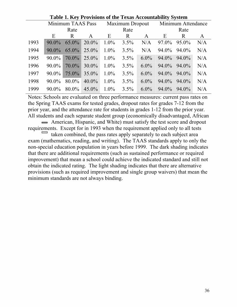
Table 1. Key Provisions of the Texas Accountability System Minimum TAAS Pass

Rate Maximum Dropout

Rate Minimum Attendance

Rate E R A E R A E R A 1993 90.0% 65.0% 20.0% 1.0% 3.5% N/A 97.0% 95.0% N/A 1994 90.0% 65.0% 25.0% 1.0% 3.5% N/A 94.0% 94.0% N/A 1995 90.0% 70.0% 25.0% 1.0% 3.5% 6.0% 94.0% 94.0% N/A 1996 90.0% 70.0% 30.0% 1.0% 3.5% 6.0% 94.0% 94.0% N/A 1997 90.0% 75.0% 35.0% 1.0% 3.5% 6.0% 94.0% 94.0% N/A 1998 90.0% 80.0% 40.0% 1.0% 3.5% 6.0% 94.0% 94.0% N/A 1999 90.0% 80.0% 45.0% 1.0% 3.5% 6.0% 94.0% 94.0% N/A Notes: Schools are evaluated on three performance measures: current pass rates on the Spring TAAS exams for tested grades, dropout rates for grades 7-12 from the prior year, and the attendance rate for students in grades 1-12 from the prior year. All students and each separate student group (economically disadvantaged, African

American, Hispanic, and White) must satisfy the test score and dropout require

exam (non-spthat theimprovobtain provisiminim

ments. Except for in 1993 when the requirement applied only to all tests taken combined, the pass rates apply separately to each subject area

mathematics, reading, and writing). The TAAS standards apply to only the ecial education population in years before 1999. The dark shading indicates re are additional requirements (such as sustained performance or required ement) that mean a school could achieve the indicated standard and still not the indicated rating. The light shading indicates that there are alternative ons (such as required improvement and single group waivers) that mean the um standards are not always binding.

36

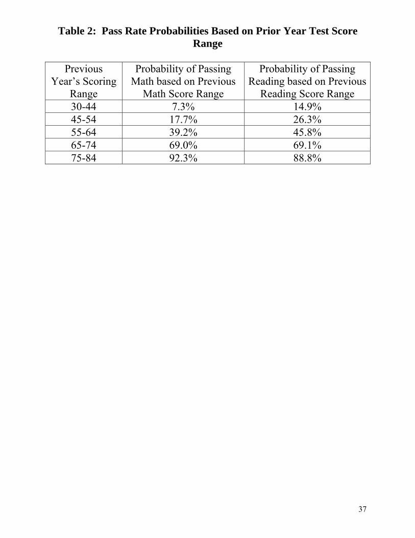
37

Table 2: Pass Rate Probabilities Based on Prior Year Test Score Range

Previous

Year’s Scoring Range

Probability of Passing Math based on Previous

Math Score Range

Probability of Passing Reading based on Previous

Reading Score Range 30-44 7.3% 14.9% 45-54 17.7% 26.3% 55-64 39.2% 45.8% 65-74 69.0% 69.1% 75-84 92.3% 88.8%

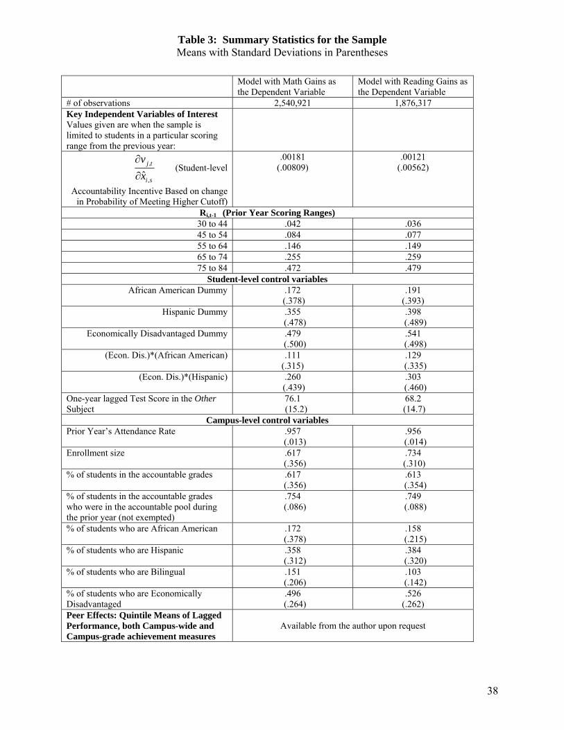
Table 3: Summary Statistics for the Sample Means with Standard Deviations in Parentheses

Model with Math Gains as

the Dependent Variable Model with Reading Gains as the Dependent Variable

# of observations 2,540,921 1,876,317 Key Independent Variables of Interest Values given are when the sample is limited to students in a particular scoring range from the previous year:

si

tj

xv

,

,

ˆ∂∂

(Student-level

Accountability Incentive Based on change in Probability of Meeting Higher Cutoff)

.00181 (.00809)

.00121 (.00562)

Ri,t-1 (Prior Year Scoring Ranges) 30 to 44 .042 .036 45 to 54 .084 .077 55 to 64 .146 .149 65 to 74 .255 .259 75 to 84 .472 .479

Student-level control variables African American Dummy .172

(.378) .191

(.393) Hispanic Dummy .355

(.478) .398

(.489) Economically Disadvantaged Dummy .479

(.500) .541

(.498) (Econ. Dis.)*(African American) .111

(.315) .129

(.335) (Econ. Dis.)*(Hispanic) .260

(.439) .303

(.460) One-year lagged Test Score in the Other Subject

76.1 (15.2)

68.2 (14.7)

Campus-level control variables Prior Year’s Attendance Rate .957

(.013) .956

(.014) Enrollment size .617

(.356) .734

(.310) % of students in the accountable grades .617

(.356) .613

(.354) % of students in the accountable grades who were in the accountable pool during the prior year (not exempted)

.754 (.086)

.749 (.088)

% of students who are African American .172 (.378)

.158 (.215)

% of students who are Hispanic .358 (.312)

.384 (.320)

% of students who are Bilingual .151 (.206)

.103 (.142)

% of students who are Economically Disadvantaged

.496 (.264)

.526 (.262)

Peer Effects: Quintile Means of Lagged Performance, both Campus-wide and Campus-grade achievement measures

Available from the author upon request

38

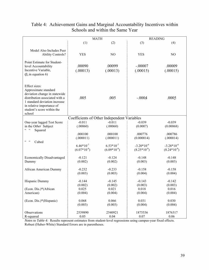
39

Table 4: Achievement Gains and Marginal Accountability Incentives within Schools and within the Same Year

MATH READING

Model Also Includes Peer Ability Controls?

(1) (2)

YES NO

(3) (4)

YES NO Point Estimate for Student-level Accountability Incentive Variable, (β in equation 6)

.00090 (.00013)

.00099 (.00013)

-.00007 (.00015)

.00009 (.00015)

Effect sizes: Approximate standard deviation change in statewide distribution associated with a 1 standard deviation increase in relative importance of student’s score within the school

.005 .005 -.0004 .0005

Coefficients of Other Independent Variables One-year lagged Test Score in the Other Subject “ “ Squared “ “ Cubed

-0.011 (.00060)

.000100

(.000011)

6.46*10-7

(6.07*10-8)

-0.011 (.00060)

.000100

(.000011)

6.53*10-7

(6.09*10-8)

-0.039 (0.0007)

.000776

(0.000014)

-3.20*10-6

(8.25*10-8)

-0.039 (0.00068)

.000786

(.000014)

-3.28*10-6

(8.24*10-8)

Economically Disadvantaged Dummy

-0.121 (0.002)

-0.124 (0.002)

-0.148 (0.003)

-0.148 (0.003)

African American Dummy -0.232 -0.233 -0.158 -0.158

(0.003) (0.003) (0.004) (0.004)

Hispanic Dummy -0.144 -0.145 -0.143 -0.142 (0.002) (0.002) (0.003) (0.003) (Econ. Dis.)*(African American)

0.025 (0.004)

0.021 (0.004)

0.018 (0.004)

0.016 (0.004)

(Econ. Dis.)*(Hispanic) 0.068

(0.003) 0.066

(0.003) 0.031

(0.004) 0.030

(0.004) Observations 2539890 2540921 1875536 1876317 R-squared 0.05 0.04 0.07 0.06 Notes to Table 4: Results represent estimates from student-level regressions using campus-year fixed effects. Robust (Huber-White) Standard Errors are in parentheses.

40

Table 5: Achievement Gains and Infra-marginal Accountability Incentives MATH READING

Includes Peer Ability Controls?

YES NO

YES NO Point Estimate for Student-level Accountability Incentive Variable, (β1 in equation 7)

.00092

(.00006)

.00119

(.00006)

.00005

(.00008)

.00057

(.00007)

Effect sizes: Approximate standard deviation change in student’s place in the statewide distribution associated with a 1 standard deviation increase in the infra-marginal incentive to help the student’s performance

.0111 .0143 .0007 .0074

Notes to Table 5: Results are based on student-level regressions including the campus-level and student-level control variables described in equation 7. Robust (Huber-White) Standard Errors are in parentheses.

41

Table 6: The Relationship between Achievement Gains and both Student-level and

Grade-level Accountability Incentives MATH READING Student-level Accountability Incentive

0.0007 (0.00006)

0.0008 (0.00006)

-0.0001 (0.00008)

0.0001 (0.00008)

Grade-level Accountability Incentive*(Lowest Achieving)

0.0061 (0.00025)

0.0064 (0.00024)

0.0015 (0.00061)

0.0027 (0.00059)

Grade-level Accountability Incentive*(Very Low Achieving)

0.0054 (0.00019)

0.0056 (0.00019)

0.0021 (0.00042)

0.0035 (0.00041)

Grade-level Accountability Incentive*(Low Achieving)

0.0051 (0.00016)

0.0053 (0.00016)

0.0021 (0.00029)

0.0030 (0.00029)

Grade-level Accountability Incentive*(Marginal Achieving)

0.0045 (0.00014)

0.0049 (0.00014)

0.0018 (0.00021)

0.0024 (0.00020)

Grade-level Accountability Incentive*(High Achieving)

0.0048 (0.00013)

0.0053 (0.00013)

0.0005 (0.00015)

0.0006 (0.00015)

APPROXIMATE EFFECT SIZES (Standard deviation change in Statewide Achievement Distribution from a 1

standard deviation increase in the Accountability Incentive) Student-level Accountability Incentive

.009 .010 -.001 .002

Grade-level Accountability Incentive*(Lowest Achieving) 0.082 0.086 0.010 0.018 Grade-level Accountability Incentive*(Very Low Achieving)

0.074 0.077 0.014 0.023

Grade-level Accountability Incentive*(Low Achieving) 0.068 0.071 0.014 0.020 Grade-level Accountability Incentive*(Marginal Achieving)

0.060 0.065 0.013 0.017

Grade-level Accountability Incentive*(Proficient)

0.061 0.067 0.004 0.005

Peer ability Controls?

YES NO YES NO

Notes to Table 6: Results are based on student-level regressions including the campus-level and student-level control variables described in equation 8. Robust (Huber-White) Standard Errors are in parentheses.