School Choice: Traditional Mechanisms and Extending the Poor’s

Ability to Choose∗

Eric Hanushek

Stanford University

Sinan Sarpca

Koc University

Kuzey Yilmaz

Koc University

September 30, 2007

∗We thank Dennis Epple, Tom Nechyba, Pat Bayer, Charles Leung, Eric Heikkila, John Quigley, James Foster,William Sander, John Merrifield, Robert Baumann, in addition to participants at the WRSA in Newport Beach, 65thMPSA, ARES in San Francisco, WEAI in Seattle, EcoMod in Brussels, APET in Nashville, and NASM at Duke fortheir comments and suggestions.

1

Abstract

We develop a multi-community urban land use framework to investigate the implications of

increasing school choice opportunities on educational and residential choices of a city’s residents.

When deciding on the location and the size of land, the households care about the distance to

the business district, and a local public good: education. There is a private education alternative

that breaks the link between choosing a residence area and choosing a school. The households

differ in their incomes and preferences for education. In five models that differ in various aspects

of choice and financing, we study the housing and education choices of the city residents, and

the endogenously determined education provision levels in equilibrium. The results of the article

support reformist arguments: We first show that the presence of a private alternative benefits

every household, whereas school district consolidation hurts everyone. We then examine two

policies that aim to increase choice. An untargeted local government support (financed by

property taxes) that can be used at the private school can improve things for talented poor. A

policy that supports the talented poor (using city income taxes) with funds that can be used for

public as well as private schools can also improve welfare of all talented students, rich or poor.

Keywords: Tiebout Model, Urban Location Model, School Choice.

JEL Classification: H4, H7, I2

1 Introduction

School choice is nothing new in United States. Long before the first vouchers were distributed

or the first charter school has opened, many American parents have been exercising choice either

by choosing where to live among different school districts, or by choosing a private alternative for

their offspring’s education. Clearly, under such a system households with higher incomes are likely

to have access to a larger opportunity set when making decisions -whether it is to relocate, or

to attend private school- and the poor and disadvantaged are usually stuck with the local public

school, with others like themselves. The discontent with the quality of public education, especially

in urban areas inhabited mostly by the latter group, lies at the heart of school choice discussions.

The reform proposals such as vouchers or charters aim to improve on the traditional mechanisms

by expanding the set of alternatives for a bigger part of the population. The resulting choice and

competition is hoped to create incentives for the inefficient public schools, raising the quality of

education for the poor and minorities also. The opponents point attention to possible undesirable

effects such as flight of talented students from public schools, deteriorating the peer quality -and

efficiency- even further.

In this paper we contribute to this ongoing debate by developing a multi-community land use

framework in which education is provided privately as well as a local (community) public good,

and when choosing a residential location households care about accessibility also. We consider five

models that differ in various aspects of choice and financing, and our results support reformist

arguments. We show that having a private alternative and autonomy in school district spending

-both of which we usually take for granted- have desirable consequences overall. We follow by

discussing the effects of two mechanisms that aim to increase the society’s ability to choose. These

mechanisms share some key characteristics with vouchers and charters, so our analysis may have

important implications to the related discussions.

In many states, decentralized financing of public education by property taxes gives school dis-

tricts fiscal and administrative autonomy. Application of Tiebout’s hypothesis predicts a competi-

1

tion between communities for residents, and a resulting sorting of households into school districts

with other households that have similar incomes and preferences for education.1 The sorting ob-

served in practice may be incomplete in reality for several reasons. First, the quality of public

education is not the only neighborhood characteristic that households care about. For example,

accessibility -one of the main determinants of residential choices in land use theory-2 is usually

ignored in Tiebout models (Two exceptions that incorporate commuting to Tiebout models are

de Bartolome and Ross (2003) and Hanushek and Yilmaz (2007)). Employment opportunities are

typically concentrated at certain locations in the city, and commuting to and from the workplace

is costly for the households. Then rents are expected to decrease as one moves away from employ-

ment locations. If land is a normal good, this will attract higher income households further away

from the city, whereas the opportunity cost of commuting time -increasing in income- will have the

opposite effect. Such issues have interesting implications on the relation between location choices

and land demands of households, which in turn relates to local property values, tax revenues, and

school district budgets.

A second reason for the partial sorting is the availability of private alternatives for education.

Private schools break the link between residential decisions and school quality, therefore are likely

to cause diversion from residential patterns implied by Tiebout’s hypothesis. For our purposes,

this is particularly important because some popular reform proposals, e.g., vouchers and charter

schools, share this characteristic. In this paper, our first goal is to understand how private schools

and their interaction with Tiebout sorting affect residential and educational choices of households.

Our second goal is to use this understanding to predict the consequences of extending the ability to

choose. Researchers have studied the provision of education and implications of reforms3 in multi-1This literature has evolved from the central insight of Tiebout (1956) and builds upon the analytical framework

developed in Ellickson (1971). The most influential studies from this approach have been conducted by Epple etal. (1984, 1993, 1998), who have also introduced politics into the model. Epple and Platt (1998) show that whenhouseholds preferences differ, the Tiebout sorting is partial and communities are heterogeneous in income.

2In the stream of literature referred to as modern urban location theory, households’ residential location is deter-mined by the trade-off between accessibility and space. The pioneer of this approach was Alonso with his model ofthe land market (1964), which was later followed by a great deal of theoretical and empirical work including those ofMuth (1969) and Mills (1972).

3See Hoxby (2003a) for a survey.

2

district models without private schooling (de Bartolome (1990), Fernandez and Rogerson (1996)),

in single district models with private schooling (Manski (1992), Epple and Romano (1998)), and

in multiple district economies with both public and private schooling (Nechyba(1999, 2000, 2003)).

Charles A.M. de Bartolome and Stephen L. Ross (2003), and Eric Hanushek and Kuzey Yilmaz

(2007) incorporate accessibility to multi-district models in which education is provided publicly. In

the first paper each household consumes the same fixed lot size. In the second paper education is

provided only publicly. Below we develop a framework that incorporates the following: 1. Tiebout

competition among two communities for residents over a local public good , education, 2. Private

alternative for education, 3. Accessibility and costly commuting, 4. Endogenous land consumption,

5. Peer effects in education. The households differ in incomes and preferences for education, and

can move freely between communities that offer different property tax-education spending packages.

Lot size is a continuous choice variable. In each community, the property tax rate is determined

by majority voting. The quality of education depends on the spending in the district as well as

some non-income characteristics of peers. We study the equilibrium with particular attention to

quality of education in public and private schools, compositions of neighborhoods, and welfare

levels of different household types. We usually do not see stratification across communities, we

observe a sorting according to the commuting distance within each community instead. The rents

that decrease in distance to the city center attracts higher income households away. A stronger

preference for housing has the same effect.

In our benchmark model, the private school selects students from the pool of households that

are willing to pay the full tuition. First, to assess the value of having a private school, we shut

down the private school and compare the equilibrium to that of the benchmark model. Next, to

understand the benefit of Tiebout sorting in the presence of a private school, we consider another

model with restricted choice, under an expenditure equalization policy. Realizing its benefits, we

consider two policies that aim to increase ability to choose via transfers to households. The first

one is an untargeted policy. The administrators in each district offer to pay up to the local per-

3

student expenditure to any local resident enrolling their kids in the private school. The second

policy targets the talented low income kids without any residency restrictions, and is financed by

city income taxes. The households can use the transfer for the private school tuition, but can also

add the transfer to the budget of a public school if they choose to attend one.

The organization of the rest of this paper is as follows: Section 2 develops the theoretical

framework. Section 3 discusses the calibration of the computable model. Sections 4.1 through 4.5

present and discuss the equilibria for five different models. Section 5 concludes.

2 The Model

We consider the residential decision making and educational choice problems of a city’s residents.

The employment opportunities in the city are concentrated in an area called the Central Business

District (CBD hereafter). Everyone that works at the CBD must choose a location to reside in

the area that surrounds it. The distance to CBD is an important factor because of the pecuniary

and time costs of commuting. A straight line that goes through the CBD divides the city into two

jurisdictions, east (e) and west (w). The jurisdictions provide a local public good, education, for

which there is also a private alternative. The (public) provision level in each locality is determined

endogenously by its residents. Therefore these jurisdictions may differ in their (property) tax and

expenditure policies, and are likely to compete for residents a la Tiebout (1956). The households

differ in their incomes and preferences for education, and the quality of education in each school

-public or private- depends on the composition of the peer group as well as the instructional

expenditures.

2.1 Households

Every household must choose a community, a residence in the community (characterized by distance

to CBD and land size), and also must choose between a private school and the public school of

the community of choice. The household supplies labor to earn an exogeneously determined hourly

4

wage W . There is a dense radial transportation system. The further one lives away from CBD,

the higher commuting costs he/she will face. In particular, if a household lives r miles away

from CBD, the cost of daily roundtrip commute will be ar dollars (pecuniary cost, a > 0) and br

hours (time cost, b > 0), which translates to bWr dollars given the opportunity cost of time. Let

l ∈ [0, 24] denote the number of non-work or leisure hours. Then the income of this household

(net of transportation costs) is Y (r) = (24− l)W − (a + bW )r.4 The households have preferences

defined over: consumption of a composite consumer good z, the land consumption (the size of the

residential lot) s > 0, leisure l ∈ [0, 24], and quality of education q at the school the offspring

attends. We assume every household has one school-age child. We normalize the price of the

composite consumption good to one and denote the unit rent of land (r miles away from CBD)

by R(r). All land is owned by absentee landlords, and the equilibrium price R(r) is determined

through a competitive bidding process, details of which we discuss below. Every household pays

a property tax with rate τ on value of land. Then, the budget constraint of a household can be

written as:

z + (1 + τ)R(r)s + Wl + p = Y (r) = 24W − (a + bW )r. (1)

The p term represents the educational expenditures whenever applicable. In particular, for those

households whose kids attend public schools, p is zero.

Households differ in their incomes (wages) and tastes for education. We name the higher income

types skilled workers (S), and the lower income types unskilled workers (U). The wages for skilled

and unskilled types are WS and WU respectively (WS > WU ). Both types exhibit variation in

their tastes for the local public good, education. Differentiating those as high valuation (H) and

low valuation (L) types gives us four types in total: SH, SL, US, and UL. Each household needs

to choose a neighborhood (east or west), a location in that neighborhood (r, distance to CBD),

amount of land to reside on (s), consumption level (z), and finally a school that the offspring

will attend. The jurisdictions operate their own public schools, and differ only in the quality of4We ignore non-commute transportation costs, and travel within the CBD.

5

education and property tax rate (qj , τj) packages. There is also a private school with quality qpri in

the city which breaks the link between choosing a community and choosing a school.

The preferences of a household can be represented by the utility function U(αi, ηi; q, s, z, l) =

qαisηizγlδ where αi + ηi + γ + δ = 1. The α parameter captures the taste heterogeneity for

education and can take on two values αi ∈ {αH , αL} such that αH > αL. Given the market rent

curves {Re(r), Rw(r)} and quality-tax packages {(qe, τe), (qw, τw)} for each jurisdiction, and quality

of education and prices for private school {qpri, pH , pL}, the household solves the problem:

maxs,z,l,j∈{e,w},q∈{qj ,qpri}

U(αi, ηi; q, s, z, l) = qαisηizγlδ (2)

s.t. z + (1 + τj)Rj(r)s + Wil + p = Yi(r)

where i ∈ {SH,SL, UH, UL}.

2.2 Schools

There are two public schools, and a private one. The public schools are neighborhood schools,

enrollment is open (and free) to residents of the community only. The existence of a private

alternative breaks the link between choosing a community and choosing a school.

The quality of education q(Π, E) in a school -public or private- is determined by (per-student)

instructional expenditures E and the peer quality Π. For a given group of students, an increase

in the instructional expenditures increases the quality of education5 (∂q/∂E ≥ 0). Also, different

groups of students may benefit differently from a given amount of instructional expenditures. That

is what the peer quality (or efficiency) component captures (∂q/∂Π ≥ 0). Some parents value

education more than others, and as a result they may spend more time helping with the kid’s

homework, provide a nicer study environment at home, be more involved in how schools operate,

etc. That is what the high valuation (H) type represents in our model, and clearly having more5There is a discussion on the effectiveness of monetary inputs on student’s achievements, but it is hard to claim

that households would not value an increase in educational expenditures.

6

students like this is in a peer group is desirable. We specify the peer quality to be increasing in the

proportion of high valuation types:

Π = c1 exp(−c2NL

N+ c3

NH

N), c1, c2, c3 ≥ 0. (3)

We divide NL and NH by N -total population- for normalization.

Public schools are neighborhood schools, admission is free, but enrollment is open to residents

of the community only. These schools are financed by property taxes on residential land. An

equilibrium property of our model is that in each jurisdiction there is a distance r∗fj called the

fringe distance beyond which no households reside. In each community entire tax revenue is spent

on education. Let L(r) denote the land density r miles away from CBD. Given the equilibrium rent

function Rj(r), and equilibrium tax rate τj , we can calculate the tax base, and total tax revenues

to find the per-student expenditure in the public school system:

Epubj =

1

Npubj

τj

∫ r∗fj

0Rj(r)L(r)dr. (4)

Note that the Npubj denotes the number of students in the public school system of community j, and

not the total number of students in the community. Everything else constant, if more households

send their kids to private schools, the per-student expenditure in the public schools will increase.

The private school is financed by tuition revenues, and can admit students from both jurisdic-

tions. Since a student’s effect on peer quality depends on whether the student is a H or L type,

it is natural for the school to condition tuition (and admission decisions) on that characteristic, if

the school can price discriminate at all. Let pH and pL denote the tuition amounts for H and L

types respectively. If NpriL and Npri

H are the number of high and low valuation types enrolled in the

private school, per-student expenditure is determined by:

Epri =pHNpri

H + pLNpriL

NpriH + Npri

L

(5)

7

The private school acts as a price taker. Given different types of households’ willingness to pay

functions, it chooses the numbers of H-types and L-types to be admitted to maximize quality of

education subject to the budget constraint (5) and a capacity constraint:

maxNpri

H ,NpriL

q = ΠE (6)

s.t. E =pHNpri

H + pLNpriL

NpriH + Npri

L

NpriH + Npri

L ≤ N

The equilibrium prices (pL, pH) are such that households’ schooling decisions are consistent with

the private school’s admission policy.

2.3 Market Rent Curves and Allocation of Land

Land is owned by absentee landlords and auctioned off to the highest bidders. The reservation

price of the landlord, Ra, is determined by an alternative use of land, such as agriculture, and is

independent of the location.

For a given utility level u we can find the maximum rent a household is willing to pay per unit

of land that is r miles away from CBD by solving the following problem:

Ψ(r, u, q, τ) = maxs,z,l

{Y − z − wl − p

(1 + τ)s

∣∣∣∣∣U(α, η; q, s, z, l) = u

}(7)

For the parametrization we use, the utility maximizing budget shares are ηi

ηi+γ+δ for s, γηi+γ+δ for

z, and δηi+γ+δ for l. Substituting these in our utility function in (2) and into the above equation

(7), we can write the indirect utility function:

V (.) =ki

R(r)ηi(1 + τj)ηiωδqαij (Yi(r)− p)(ηi+γ+δ) (8)

8

and the bid rent function:

Ψ(r, u, q, τ) =k

1/ηi

i

(1 + τj)ωδ/ηiqαi/ηi

j (Yi(r)− p)(ηi+γ+δ)/ηiu1/ηi

i (9)

where ki = ηηii γγδδ

(ηi+γ+δ)ηi+γ+δ is a constant. We are interested in the shapes of these bid rent functions.

The negative slopes of bid rent curves:

∂Ψ∂r

= −Ψ(.)ηi + γ + δ

ηi

a + bWi

Yi(r)− p< 0,

indicate that all types of households are willing to pay lower rents as they move away from CBD.

Also the bid rent curves are strictly convex for every type (∂2Ψ/∂r2 > 0).

At an auction for a particular location r∗, the winner will be the type with the highest bid rent

curve at that location. Given the four types in the model, and given that each type has a choice

over private and public schools, in each jurisdiction we can plot eight different bid rent curves. The

equilibrium rent curve Rj(r) will be the upper envelope of the bid rent curves of different types and

the agricultural rent Ra. Because all bid rent curves are convex and decreasing, the equilibrium

rent curve Rj(r) will be decreasing up to a distance r∗jf , the fringe distance, and will stay constant

from that point on, because the agricultural rent will exceed every household’s willingness to pay

for land. In our computational analysis we check and verify that two different types’ bid rent curves

can intersect at one point at most. This single-crossing property of bid rent curves proves quite

useful for our analysis. Households with steeper bid rent curves will locate closer to the CBD. To

understand the relation between the slope of the bid rent curve and the income and preferences of

a household, suppose bid rent curves of two households intersect at r∗, i.e., Ψ(r∗, u1) = Ψ(r∗, u2).

Some algebra indicates that Ψ1 is steeper than Ψ2 if and only if

∀r, (η1 + γ + δ)η2

(η2 + γ + δ)η1

a + bW1

a + bW2

Y2(r)− p

Y1(r)− p> 1.

Consider two households with same incomes but different tastes for education. Suppose the ed-

9

ucation expenditure p is same for both. If both locate in the same jurisdiction, above equation

implies that high valuation (αH) types will locate closer to CBD. Since low valuation households

attribute relatively more weight to land, they will locate further away from CBD where rents are

cheaper. For two households with same preferences and different incomes, the answer is not that

clear. Higher income increases the demand for land consumption and attracts households further

away from CBD, but it also increases the opportunity cost of commuting time. To understand

which effect is dominant, we will use computational models below. Attending the private school is

equivalent to an income reduction by an amount p, hence the above income discussion applies.

2.4 Population

Our city is a closed city, population is given exogenously. Let L(r) denote the land density r miles

away from CBD, and let nj(r) denote the equilibrium density function of the household population

in jurisdiction j. Suppose in equilibrium the residents of the land at distance r in jurisdiction j are

type i households. Then nj(r) = L(r)s(r,u∗i ,.) . Let NSH , NSL, NUH , and NUL stand for the populations

of the respective types. The population constraint for each type i ∈ {SH, SL,UH, UL} can then

be stated as: ∫ ∞

0

L(r)sw(r)

I[t∗w(r) = i]dr +∫ ∞

0

L(r)se(r)

I[t∗e(r) = i]dr = Ni (10)

where t∗j (r) is a function showing the type of the occupant at distance r in jurisdiction j, and I[.]

is an indicator function that takes the value 1 when the condition in brackets is satisfied, and 0

otherwise. The population constraint implicitly assumes the land market clears in each jurisdiction:

∀r ≤ r∗fj , Sj(r)nj(r) = L(r).

2.5 Local Public Finance

The two jurisdictions differ only in the quality of education and property tax rate (qj , τj) packages

they provide. In each locality taxes are determined by majority voting. The households are myopic

10

in the sense that when voting, they do not consider the migration patterns and the resulting changes

in composition of neighborhoods the outcomes can cause. We focus on the stationary equilibrium,

which is attained when no one has an incentive to relocate in response to the voting results.

When choosing a community, households take the tax-expenditure packages as given. They

move in and vote for the property tax rate. For a household that chooses the public school the

preferred tax rate is the one that solves the problem:

τ∗i = argmaxτ

V (.) =ki

(1 + τj)ηiR(r)ηiωδqαij (Yi(r)− p)ηi+γ+δ s.t. qj = ΠjEj (11)

and Ej = τjRj

Note that the most preferred tax rate τ∗i = αiηi−αi

is independent of income. Clearly, for households

that choose the private school, most preferred tax rate is zero, and they will always locate in the

lower tax neighborhood.

Definition (Equilibrium): An equilibrium is a set of utility levels for each type {u∗SH , u∗SL, u∗UH , u∗UL},

market rent curves for each jurisdiction {Re(r), Rw(r)}, quality of education and property tax rate

pairs {(qe, τe), (qw, τw)}, quality of education and prices for private school {qpri, pH , pL}, household

population distribution functions {ne(r), nw(r)}, and type functions {t∗e(r), t∗w(r)} that show the

equilibrium locations of the occupants at distance r in community j such that:

• Households’ choices are determined by solving (8).

• The market rent function Rj(r) in each jurisdiction is determined through a bidding process

among different types of households

• Same types of households obtain the same level of utility regardless of their choices.

• The private school’s admission policy solves (6).

• The tax rates in each jurisdiction are determined by majority voting by myopic voters.

• Local governments’ budgets balance in each jurisdiction.

• Labor and land markets clear.

11

• The population constraints (10) hold.

3 Calibration

The complexity of our model induces us to proceed with computational analysis. We specify the

parameters of the computational model(s) to match certain statistics from U.S. data.

In the previous section, we have identified the utility maximizing budget shares for leisure,

consumption, and lot size as δηi+γ+δ , γ

ηi+γ+δ , and ηi

ηi+γ+δ respectively. In U.S. average hours of

work per week in full time jobs is 40 hours, and average annual earnings of workers are $22,154

for high school graduates and $38,112 for college graduates. Accordingly, we set the hourly wages

for unskilled and skilled types as WU = 15 and WS = 21. In a 168(=24*7) hour week, 40 hours

of work implies a 0.762 budget share for leisure. The data on household expenditures suggest that

expenditures on shelter constitute about 20% of the budget of an average household. This implies

budget shares of 4.76% for housing and 19% for consumption. There are two possibilities for the

most preferred tax rates according to (11). We set these most preferred tax rates equal to 2.2%

(1.6%) for the high (low) valuation types. The utility function parameters consistent with all these

are αL = 0.014, αH = 0.016, δ = 0.75, and γ = 0.2

We calculate the commuting costs assuming the households drive to work. The pecuniary cost

can be calculated based on the cost of owning and operating an automobile. In 2004 pecuniary

cost per mile was $ 0.56, and we set a = 1.1. Assuming the commuting speed in the city is 20 miles

per hour, we set b = 0.13. We assume 2 million households populate the city. When computing

the equilibrium, we target for a (endogenous) fringe distance (city radius) around 15 miles in each

jurisdiction. The proportion of skilled households in U.S. is about 30%. We expect this proportion

to be slightly higher in a city. Hence, we set the proportion of skilled households to 40%, about

30% of which are low valuation types. We want the proportion of low valuation types among the

unskilled to be higher and set that equal to 70%.

12

Studies report the proportion of students in private schools around 10%.6 We assume the private

school can accommodate 12% of all students. We set the parameters of the school quality function

to match some empirical facts as c1 = 4.06, c2 = 3.35, and c3 = 0.26.

4 Results

First we discuss the equilibrium of the benchmark model with one private school and two (au-

tonomous) public schools. We follow by two models that investigate the benefits of the traditional

choice mechanisms. To restrict the alternatives set, we first look at the case where there is no

private school. Then we analyze the consequences of consolidating the two school districts in the

presence of a private alternative. In two other models we study the effects of two different “money

follows student” programs, where eligible households are offered transfers to be used at the school

of their choice. In the first one, every household has the option to receive a transfer -as high as

the per-student expenditure at the local public school- to be used for the tuition at the private

school. This is paid out of the district’s budget (local property tax revenues). The second program

provides a transfer from the central government to low-income households anywhere. This transfer

can also be added to a public school’s budget, and is financed by (city) income taxes. Several key

properties of equilibrium exhibit big variation from one model to another, below we discuss the

common features first.

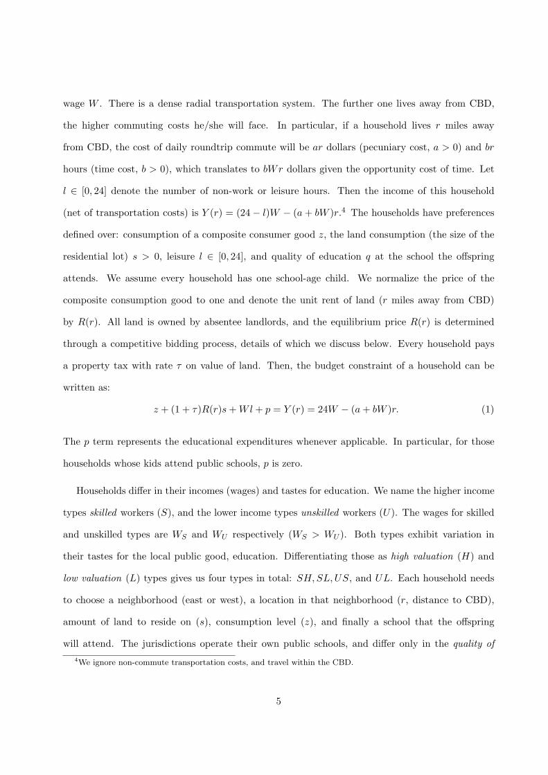
The welfare comparisons of the four models are summarized in Table 1. The unit of measurement

is the percentage change in rent required to keep the relevant types of households at their equilibrium

utility level in the benchmark model. A negative number means the household is worse off. A quick

look at the table shows that restricting choice hurts every household in the city (columns 1 and

4), whereas programs that are designed to increase choice may help all high valuation types or

unskilled high types, at the expense of rest (columns 2 and 3). We discuss all these in further detail

below.6See Epple and Romano (1998), School District Data Book 1990, as well as the NCES report titled ”Characteristics

of Private Schools in the United States: Results From the 2003-2004 Private School Universe Survey.”

13

Table 1: Welfare Analysis.

Type Pubonly PoorChoice Incometax Consolid.

Skilled High -0,0887 -2,0507 0,1440 -8,8147

Skilled Low -0,0219 -1,0309 -0,2069 -7,4035

Unskilled High -0,0862 1,0364 1,9645 -9,1897

Unskilled Low -0,1586 -1,6476 -0,0708 -7,4933

AEU -0,1066 -1,1488 0,3477 -7,9737

In all models, we observe communities that are heterogeneous in income. This is consistent

with empirical findings (Davidoff (2005)) as well as results of theoretical studies including Tiebout

models such as Epple and Platt (1998), and Tiebout-Urban hybrid models such as Hanushek and

Yilmaz (2007).

The market rents in each jurisdiction decrease as one moves away from the CBD in all models

we consider below. This is an implication of costly commuting. The land allocation patterns are

quite similar across different models too. Each jurisdiction is partitioned by several semi-rings that

have CBD at the center. This “rings” structure dates back to von Thunen’s model of land use

(1826), and is one of the building blocks of Urban Land Use Theory. In our models we have semi-

rings instead of full ones because of the jurisdiction boundaries, or the local public goods problem.

As a result, the widths and numbers of rings may show variation in two localities. The ordering

of households around CBD however, is same in every model. We had discussed earlier that high

valuation households will always locate closer to the CBD compared to the low valuation types

at the same income level. Because in their utility functions, low valuation types assign relatively

higher weights to land. Similarly, among households with same valuation, higher income increases

the land demand and attracts households further away from CBD where the land is cheaper. High

income also increases the opportunity cost of commuting time. But our results show that this

effect is dominated by the former, and the ordering of households in each district in every model

14

is as follows: The UH types locate closest to the CBD. The UL types occupy the semi-ring that is

outside that of UH types. As we move further away from CBD we see SH types first followed by

SL types. Sometimes a particular type may not be present in a district. But the order between the

others is still preserved. The outer end of the SL ring is the fringe distance and the land beyond

that is left for agricultural use.

The distribution of SL type households across two localities remain stable in all models, but

the distributions of the other three types exhibit big variations. The private school’s student

composition changes too, and those who attend the private school always choose to locate in the

lower tax neighborhood. Since private school attending types do not receive any benefit from the

tax revenues, they have no incentive to pay any.

4.1 Benchmark Model

Figure 1 and Table 2 illustrate some important equilibrium properties of the benchmark model.

Without loss of generality, we will refer to the higher tax neighborhood as east school district

throughout the rest of this paper. In the figure the equilibrium rent functions Rj(r) in each juris-

diction are given by the lines, and the distribution of population within and across the communities

is shown using bars. All four types of households can be observed in both localities. Only the skilled

high types attend the private school, and the SH type households that choose private school are

the only SH types that locate in the lower tax neighborhood. The private school does not have any

students that reside in the east.

The quality of education is higher in the east, the district with higher taxes. Note that per-

student expenditure in the west school district is higher. There is a group of high income residents

that contribute significantly to the district’s budget, but do not claim any of the revenues since

their kids attend the private school. This increases the per-student expenditure for those at the

public school. However, higher expenditures fail to provide a higher quality. The private school

attending students are desirable (high valuation) peers, and with them being out of the peer group

15

the public school consists of low valuation types mostly.

Table 2: Benchmark Equilibrium

West East Private

quality 10.9 14.2 23.4

expenditure $ 2701.4 $ 2413.9 $ 2040.2

tax 1.6 % 2.2 %

In the absence of a private schooling alternative, the higher tax community provides a higher

quality of education with higher per-student-expenditure (see Section 4.2 and Hanushek and Yilmaz

(2006)). This could easily mislead one to overrate the role of expenditures on school quality. Also,

the expenditures at the private school is lower than both public schools, but the peer quality is

very high. As a result, the quality in the private school is at a maximum among all models we

consider in this paper.

With this price tag, private school is not an affordable option for unskilled types. As a result,

most low income-high valuation (UH) type households choose to live in the east -despite the higher

rents- because of the higher quality of public education. For low income-low valuation type house-

holds, the lower-taxes in the west balances the lower quality of education, and their distribution

across communities is more balanced in every model we consider here.

4.2 The Value of Having a Private Alternative

In the benchmark model we take the private alternative for granted. However, we are certainly

interested in understanding who is affected -and how- from having such an option.7 So we analyze

the equilibrium in the city without a private school, the traditional case in which school choice can

be done only through community choice.8 Table 2 compares the quality and expenditures at schools7Competition between public and private schools is analyzed in a single community framework in Epple and

Romano (1998).8Fernandez and Rogerson (1996) consider such a model in which public education is financed by income taxes.

16

in two communities. The quality in the east reaches a maximum among all models. However, the

quality in the lower-tax neighborhood hits the minimum level among all models, and so does the

quality difference between two neighborhoods. We see a similar effect on rents. We discuss the

implications of the rent gap on households choices and welfare in detail below. Having private

schooling seems to have benefits to a group larger than its students.

Table 3: Public Schools Only

West East

quality 6.4 18.7

expenditure $ 2012.3 $ 2426.6

tax 1.6 % 2.2 %

The huge quality difference between two districts cannot be attributed to the (disproportionate)

difference in per-student expenditure. The quality difference is mostly due to the differences in peer

quality -or population composition- across the two districts. An inspection of Figures 8 through

11 makes this pretty clear. The high income households sort themselves into two neighborhoods

according to their preferences for education: All the SH types locate in the east, and all the SL

types locate in the west. We see a similar -but partial- sorting among low income households too.

All the UH types locate in the east. Although we observe UL types in both jurisdictions, a larger

proportion resides in the west. This model’s equilibrium exhibits the strongest sorting based on

preferences.

Comparing this model with the benchmark, we can summarize the benefits from having a private

school as follows: A private school weakens the Tiebout sorting and allows some high income house-

holds with strong preferences for education to choose residences in the areas that have relatively

lower quality public schools, and lower taxes. These parents increase the per-student expenditure

in the district by paying taxes higher than the typical resident, and also by not claiming (or by

redistributing) their share of local expenditures since their children attend the private school. As

17

a result, the other residents of these districts can have a higher quality in public schools than they

could in the lack of the private school.

On average, the UH (SH) types pay taxes that are less (more) than per student expenditure.

Now the east school district consists of UH and SH types only. More UH types in the neighborhood

means a bigger burden on SH types. The peer quality increases with UH exchanging places with

SL in the public school, and this shows in the school quality. However, the increase in rents and

tax expenditures outweighs the increase in quality at the school and SH types end up worse off. In

the benchmark, the contribution of private school attending SH residents was a major determinant

of UH types choosing to live in west. With that out of the picture, the UH types move to east for a

better education. However, the increase in quality of education fails to compensate for the higher

rents and taxes for them too. The rents decrease in west school district, and so does the quality of

education. The residents are (skilled and unskilled) low valuation types exclusively. However, the

decline in the quality of education is so dramatic, it outweighs the gain from rents and taxes. In

equilibrium every household is worse off compared to benchmark model.

4.3 A Spending Equalization Program

School district consolidation is a policy motivated by economies of scale, and it aims to increase

efficiency of public schools by cutting costs. Over the last several decades, the number of school

districts has decreased dramatically in United States, and the proponents demand further consol-

idations. In this paper our focus is on the allocation rather than the technology. Our framework

allows us to study the distribution of households across districts and across schools, and the result-

ing education provision levels when spending is restricted to be equal everywhere.

The typical outcome in local public goods models is that households group with others that have

similar preferences and income levels, or similar willingness to pay. In our framework, preferences

affect the provision level not only through local residents’ willingness to pay, but through peer

effects too. We saw in Section 4.2 that most high valuation types stick together and pay higher

18

rents and taxes. Also remember that quality of education for a given expenditure level increases

in the proportion of high valuation types in the peer group. As a result both the spending and the

peer quality in their district exceeds those in the other. The benchmark model in 4.1 illustrates the

distortion on this sorting caused by private school. Private school attending households chose to live

in the west community where rents and taxes are lower. This increases the per-student expenditure

in the district, however fails to increase quality proportionally. In this section we study households’

choices when we close the willingness to pay channel, in the presence of a private school.

Table 4: Consolidation

West East Private

quality 8,1 11,8 12,7

expenditure $ 2004,6 $ 2004,6 $ 1104,5

tax 1.6 % 1.6 %

Table 4 displays the equilibrium outcomes. Both the quality of education and the per-student

expenditures at public schools are lower than those at the benchmark equilibrium. Moreover, the

quality difference between two public schools is slightly larger compared to benchmark. This low

quality of public education in both localities makes the private school much more attractive to all

high valuation types. The unskilled cannot afford the tuition, but the harder competition among

skilled high valuation types causes a lower equilibrium tuition/expenditure level for the private

school. As a result, we see the most dramatic effect of this policy on the quality of private school.

Note that it is not the peer quality that is affected, the private school still consists of SH types

only. But the quality implied by the low expenditure level exceeds the quality of the east public

school only slightly.

Consolidation weakens high valuation households’ incentives to live in the east. The city consists

of only one district now, and the low valuation types constitute the majority. Therefore the voting

outcome is the lower tax rate. Combined with the decrease in rents in both commodities, this

results in lower tax revenues overall which explains the low expenditures. In the benchmark model,

19

households determined quality of education through instructional expenditures and peer effects.

But now they are left with only the latter, hence cannot be as effective on provision levels. Also in

the benchmark model, the tax revenues from private school attendees that live in the west contribute

to the budget of public school students in the west only. Many unskilled high valuation types choose

to live there because of the resulting high per-student-expenditure. Under a consolidation policy,

those revenues will be split between two districts. This will affect the incentives of UH type

residents, and some will move to east. The burden on the skilled residents of the east increases,

since they will subsidize more unskilled types now.

The combined effects not only decrease the rents in both jurisdictions, but also narrow the rent

gap between the communities. East housing is relatively cheaper compared to the benchmark,

and this attracts some new residents - particularly SL types. Despite the decrease in quality of

education, every household will benefit from the decrease in rents and tax payments. To see which

effect dominates, we conduct a welfare analysis in Table 1. As summarized in the last column,

shows that the impact of expenditure equalization is not only negative for everyone, but also huge

in magnitude compared to the welfare changes in the other models above. In our economy low

valuations types are the majority so the outcome represents their preference. This hurts high

valuation types and triggers a chain of events -some of which we described above- which in turn

hurt also the rest in equilibrium.

4.4 An Untargeted Program Financed by Property Tax Revenues

The analysis in the previous sections suggests that having a larger opportunity set has desirable

consequences not only for the households who choose the higher spending neighborhood or the

private school, but for the society in general. Clearly high income households have more flexibility

when making decisions -whether it is to relocate, or to attend private school- and low income

households have very limited options, if any. Public administrators may be interested in increasing

the access for the low income families as well. In practice this would be desirable not only in

20

terms of fairness and equality, but also in terms of increasing school competition and efficiency. If

choice is beneficial, then the effects could be amplified as the number of people that exercise choice

increases. In this section and next, we investigate the consequences of two programs that aim to

enable more people to make choices.9

In our framework, the jurisdictions collect property taxes, and spend the revenues as educational

expenditures in the public school system (see (4)). Let’s say each household living in jurisdiction

j is entitled to an expenditure of Vj dollars from the district’s budget. Instead of spending this

money in public schools on behalf of the households, suppose the administrators offer the local

residents the option to use up to Vj dollars from the district’s budget, to pay tuition at the private

school:

Vj = max{p,Epubj }, j ∈ {e, w} (12)

Of course this offer is conditional on being admitted at the private school. The households can

add on top if the tuition p exceeds the transfer amount. The school quality implications of this

policy can be seen in Table 5. The quality difference between the two public schools increases. The

school in the east (west) has higher (lower) quality compared to the benchmark equilibrium. The

expenditures are very close, so the quality difference can be attributed mainly to the differences in

composition of population between two localities.

Table 5: Choice to the Poor

West East Private

quality 8.5 16.1 9.9

expenditure $ 2314 $ 2513 $ 859

tax 1.6 % 2.2 %

9One such mechanism proposed by school choice proponents to increase choice -especially for the low incomehouseholds- is vouchers (For effects of vouchers see Manski (1992), Epple and Romano (1998), Rangazas (1995), Hoytand Lee (1998), Nechyba (1999, ), Nechyba (2003).) Vouchers can be unconditional, or eligibility and its amount canbe conditioned on some student characteristics (income, ability) or school characteristics (tuition), and different typesof vouchers would cause different distributions of students across schools. Voucher design is a very interesting problem(see Epple and Romano (2003b), Necyba (2000), Caucutt (2002)). The mechanism we consider in this section canbe thought as a flat-rate voucher, to which every household is eligible.

21

The quality in the private school is very low, almost as low as the public school in the west. The

student composition has changed completely. Unlike benchmark model, no SH types exist in the

private school, and it consists of UH types only. The peer quality did not diminish, all students

are still high valuation types, so quality decline is caused by the big reduction in per-student

expenditure. For efficiency purposes, the private school should needs to charge a higher tuition

for low valuation types because of their negative effect on peer quality. But low valuation types

are not willing to pay higher than high valuation types. So the competition for the private school

seats is between UH and SH types really, and they will both bid for a residence in the west. For a

UH type, a private school spending/tuition up to Epubw -the per-student expenditure in west public

school- comes at no cost, whereas SH types have to pay the full amount. With this advantage, UH

types outbid SH guys. Their high demand keeps the equilibrium tuition/spending at the private

school at a very low level. At the same time east becomes more attractive for SH types, because

of the move of a significant number of UH types who would live in east and pay relatively less.

Their spending in the east is more effective now, so they spend more and the resulting quality of

education is higher than the benchmark.

Our welfare analysis shows that the unskilled high valuation types do benefit from this policy,

but the other three types of households end up worse off compared to the benchmark model.

4.5 A Targeted Program Financed by Income Tax Revenues

The program we have considered in the previous section is is untargeted - any household is eligi-

ble. However, earlier we had argued that lower income households are the ones that really face

restrictions on alternatives and choice. And among them, the high valuation types are more likely

to make use of such a transfer. Our findings in the previous section verify these. The UH types use

the transfers and replace the SH types in the private school. If UH types are the clientele, then it

may be desirable to design a program that targets them exclusively.

More important, in Section 4.4 each district offers a locally financed transfer to its own residents.

22

But we have also learned that a household that chooses the private school will live in the west school

district where the tax rates (and most likely rents and expenditures too) are lower. Therefore it

does not really matter whether the east offers the same program or not, because the burden of the

program is on the west residents really. This is particularly unfair if the west is poorer. In the

benchmark, the private school attendees are SH types exclusively. In 4.1 we have discussed the

importance of their contribution to the public school expenditures. When UH types replace them

in 4.4, the public school attending residents in west lose this contribution and face the burden of

the private school at the same time. Finally, the program in 4.4 increases ability to choose for UH

types that attend the private school, however does not provide any direct benefits for the remaining

UH types.

The problems we have just described motivate us to study the effects of a program that targets

UH types exclusively and treats them equally, while distributing the burden throughout the city

rather than the lowest tax community only. Specifically, the city collects income taxes to finance a

transfer to all the unskilled high valuation type residents in any locality. We denote the (exogeneous)

city income tax rate by t. The budget of a typical household is then:

z + (1 + τ)R(r)s + p = (24− l)(1− t)W − (a + b(1− t)W )r.

In addition to all the standard effects of an income tax, note that we observe a decrease in com-

muting costs because of the decrease in opportunity cost of time. The total income tax revenue is

distributed equally among all eligible households. The households can then take this money and

use it for private school tuition, contributing on top if necessary. Alternatively, the households may

attend the public school of their choice, and add the transfer amount to that school’s budget. If

V denotes the per-household transfer amount, and NUHj denotes the number of UH types in the

public school system of community j, the budget of the district (the counterpart to (4)) will look

23

like:

Epubj =

1

Npubj

[τj

∫ r∗fj

0Rj(r)L(r)dr + NUH

j ∗ V]

(13)

There is no difference between SH and UH types in terms of peer quality. In the previous models

SH types were more desirable neighbors than UH types because of their higher contribution to tax

revenues. This program may increase UH types’ contributions to the local budgets, and make them

more desirable students in every community. We choose the income tax rate (0.26%) so that the

private school no longer consists of a single type of students. When we increase (decrease) the tax

rate, the proportion of UH (SH) types increases and reaches 1 eventually.

Table 6: Choice to the Poor 2

West East Private

quality 9,7 16,8 17,0

expenditure $ 2647,3 $ 2586,1 $ 1483,2

tax 1.6 % 2.2 %

Some key properties of equilibrium are given in Table 6. The school in the east (west) has higher

(lower) quality compared to the benchmark equilibrium, and the quality of private school is lower

than that in benchmark just like in the previous exercise. But the quality of education in every

school is higher compared to those in the previous section.

We see both UH types and SH types in the private school, the proportion of the first group

being slightly higher. High-valuation types -skilled or unskilled- either live in the east, or attend

private school. West rents are significantly lower compared to the benchmark, whereas rents in

east decrease only slightly. Those SH types that are replaced by UH types in the private school

move west. That does not hurt the expenditures much because of a few reasons. Because of the

low rents we see a migration of SL types from east to west which partially compensates decrease

in SH population. Second, the burden is no more on west residents only unlike the program in

4.4. Third, the total number of public school students in west decreases, increasing per-student

24

expenditure. Finally, the decrease in west rents increase a typical household’s lot size, causing the

neighborhood and the taxable land to expand. As a result the peer quality and the expenditures in

west decrease only slightly, causing a small decrease in school quality compared to the benchmark.

The UH types that do not attend the private school live in east. They contribute to district’s

budget not only through property taxes, but also through the program’s transfers as well. The

SH population in the east increases too. The program decreases the burden of UH types on SH

types, and SH money is more effective now. The resulting expenditure level in east exceeds the

benchmark level, and so does the peer quality. The quality of education in east is higher compared

to the benchmark. The improvement on school qualities over 4.4 decreases the private school

demand, and the implied tuition/expenditure level is higher in this model’s equilibrium.

All high valuation types benefit from this policy, the welfare change to the unskilled being higher.

As a measure of total welfare in the economy we calculate an index, a normalized sum of household

utilities, and call it Aggregate Expected Utility (AEU). Among the four models we consider, this

policy is the only one that is an improvement over the benchmark in terms of AEU.

5 Concluding Remarks

We have introduced a private schooling alternative in a two-community city, and illustrated under

different conditions how it alters the residential and educational choices as well as opportunity

sets of different types of households. The concern for accessibility enriches the Tiebout framework

through its implications for the relation between location choices and land demands of households,

which in turn relate to property values, tax revenues, and school district budgets. A particularly

interesting finding is the severed link between expenditures on school quality (4.1 and 4.5). Another

one follows from the experiments in which we restrict alternatives: Having a larger opportunity set

has benefits not only for the households that select choose those alternatives, but for the remaining

as well. The lack of private schooling caused a disturbingly low quality of education in the poorer

neighborhood, and expenditure equalization caused fairly large welfare losses to every resident.

25

Concerned by the inequality of opportunities between the rich and poor when choosing schools,

we have considered two very simple mechanisms to extend the ability for the latter. Our results

point to the desirability of central financing as opposed to local. We can draw some lessons from

these experiments about the market implications of popular reform proposals such as vouchers and

charters. Our future work will study these issues in greater detail.

References

Alonso, William. 1964. Location and land use. Cambridge, MA: Harvard University Press.

Bearse, Peter; Glomm, Gerhard and Ravikumar, B. Majority Voting and Means-Tested Vouch-ers. Working Paper, Michigan State University, 2001.

Caucutt, Elizabeth. Educational Policy When There Are Peer Group Effects Size Matters.International Economic Review, February 2002, v. 43, pp. 195-222.

Cohen-Zada, Danny and Justman, Moshe. The Religious Factor in Private Education. Journalof Urban Economics, May 2005, 57(3), pp. 391-418.

Davidoff, Thomas. 2005. ”Income Sorting: Measurement and Income Decomposition.” Journalof Urban Economics 58, no.2 (September):289-303.

de Bartolome, Charles A. M., and Stephen L. Ross. 2003. ”Equilibria with local governmentsand commuting: Income sorting vs income mixing.” Journal of Urban Economics 54:1-20.

Ellickson, Bryan. 1973. ”A generalization of the pure theory of public goods.” American Eco-nomic Review 63, no.3 (June):417-432.

Epple, Dennis, Radu Filimon, and Thomas Romer. 1984. ”Equilibrium among local jurisdic-tions: toward an integrated treatment of voting and residential choice.” Journal of Public Economics24, no.3 (August):281-308.

Epple, D., and Romano, R. (1998). Competition Between Private and Public Schools, Vouchersand Peer Group Effects. American Economic Review, 88, 33-63.

Epple, Dennis, Radu Filimon, and Thomas Romer. 1993. ”Existence of Voting and Hous-ing Equilibrium in a System of Communities with Property Taxes.” Regional Science and UrbanEconomics 23:585-610.

Epple, Dennis, and Thomas Nechyba. 2004. ”Fiscal decentralization.” In Handbook of Regionaland Urban Economics, edited by J. Vernon Henderson and Jacques-Franois Thisse. Amsterdam:Elsevier:2423-2480.

26

Epple, Dennis, and Glenn J. Platt. 1998. ”Equilibrium and Local Redistribution in an UrbanEconomy when Households Differ in both Preferences and Incomes.” Journal of Urban Economics43, no.1 (January):23-51.

Epple, Dennis and Romano, Richard. 2003a. ”Neighborhood schools, choice and the distributionof educational benefits.” In The Economics of School Choice, edited by Caroline M. Hoxby. Chicago,IL: University of Chicago Press.

Epple, Dennis and Romano, Richard. 2003b. Educational Vouchers and Cream Skimming,Working Paper, University of Florida.

Fernandez, Raquel, and Richard Rogerson. 1996. ”Income distribution, communities, and thequality of public education.” Quarterly Journal of Economics 111,no.1 (February):135-164.

Friedman, Milton. 1962. Capitalism and Freedom. Chicago : University of Chicago Press.

Fujita, Masahisa. 1989. Urban Economic Theory: Land Use and City Size. New York, NY:Cambridge University Press.

Hanushek, Eric A. 2003. ”The failure of input-based schooling policies.” Economic Journal 113,no.485 (February):F64-F98.

Hanushek, Eric A., John F. Kain, Jacob M. Markman, and Steven G. Rivkin. 2003. ”Does peerability affect student achievement?” Journal of Applied Econometrics 18,no.5 (September/October):527-544.

Hanushek, Eric A., John F. Kain, and Steve G. Rivkin. 2004. ”Disruption versus Tieboutimprovement: The costs and benefits of switching schools.” Journal of Public Economics Vol 88/9-10:1721-1746.

Hanushek, E. and F. Welch ed. 2006. Handbook of the Economics of Education, Volume 1, 2,Elsevier.

Hanushek, E. and K. Yilmaz. 2007. ”The complementarity of Tiebout and Alonso”, Journal ofHousing Economics, forthcoming.

Hoxby, Caroline M. 2001. ”All school finance equalizations are not created equal.” QuarterlyJournal of Economics 116,no.4 (November):1189-1231.

Hoxby, Caroline M. ed. 2003a. - The Economics of School Choice, Chicago, IL: University ofChicago Press.

Hoxby, Caroline M. 2003b. - School Choice and School Productivity: Could School Choice bea Tide that Lifts All Boats? In The Economics of School Choice, edited by Caroline M. Hoxby.Chicago, IL: University of Chicago Press.

Hoxby, Caroline M. 1998. - What Do Americas ”Traditional” Forms of School Choice TeachUs about School Choice Reforms? - Federal Reserve Bank of New York Economic Policy ReviewMarch, 47-59.

27

Hoyt, W., and K. Lee. 1998. ”Educational vouchers, welfare effects, and voting”, Journal ofPublic Economics. 69, 211228.

Manski, C. 1992. Educational choice (vouchers) and social mobility, Economics of EducationReview 11, 351369.

Leung, Charles. 2004. ”Macroeconomics and Housing: a review of the literature,” Journal ofHousing Economics, 13, 249-267.

Nechyba, Thomas J. 1999. ”School Finance Induced Migration Patterns: The Impact of PrivateSchool Vouchers,” Journal of Public Economic Theory. 1, no. 1, 5-50, January 1999

—. 2000. ”Mobility, targeting, and private-school vouchers.” American Economic Review 90,no.1 (March):130-146.

—. 2003. ”Public school finance and urban school policy: General versus partial equilibriumanalysis.” In Brookings-Wharton papers on Urban Affairs, 2003, edited by William G. Gale andJanet Rothenberg Pack. Washington: Brookings:139-170.

—. 2003. Introducing School Choice into Multi-District Public School Systems, in CarolineHoxby, ed., The Economic Analysis of School Choice. Chicago, IL: University of Chicago Press.

—. 2003. ”Centralization, Fiscal Federalism and Private School Attendance,” InternationalEconomic Review 44(1), 179-204.

Rangazas, Peter. 1995. Vouchers and Voting: An Initial Estimate Based on the Median VoterModel, Public Choice, Vol. 82, 261-279.

Tiebout, Charles M. 1956. ”A pure theory of local expenditures.” Journal of Political Economy64, no.5 (October):416-424.

U.S. Bureau of the Census. 1994. County and City Data Book 1994. Washington, D.C.: U.S.Dept. of Commerce

—. 1998. Statistical abstract of the United States: 1998. Washington, DC: U.S. GovernmentPrinting Office.

U.S. Department of Education. 2004. Digest of Education Statistics, 2003. Washington, DC:National Center for Education Statistics.

28

Figure 1: Monthly Gross Market Rent (per acre) Rent

0

2000

4000

6000

8000

10000

12000

14000

16000

18000

-12 -10 -8 -6 -4 -2 0 2 4 6 8 10 12

Location

0

5

10

15

20

25PopulationSkilled LowSkilled HighSkilled High PrivUnskilled LowUnskilled High

Fig 7: Quality of Education

0,0

5,0

10,0

15,0

20,0

25,0

Bench Pubonly PoorChoice Incometax Consolid.

WestEastPriv

Fig 6: Expenditure per Pupil per year

0,0

500,0

1000,0

1500,0

2000,0

2500,0

3000,0

Bench Pubonly PoorChoice Incometax Consolid.

WestEastPriv

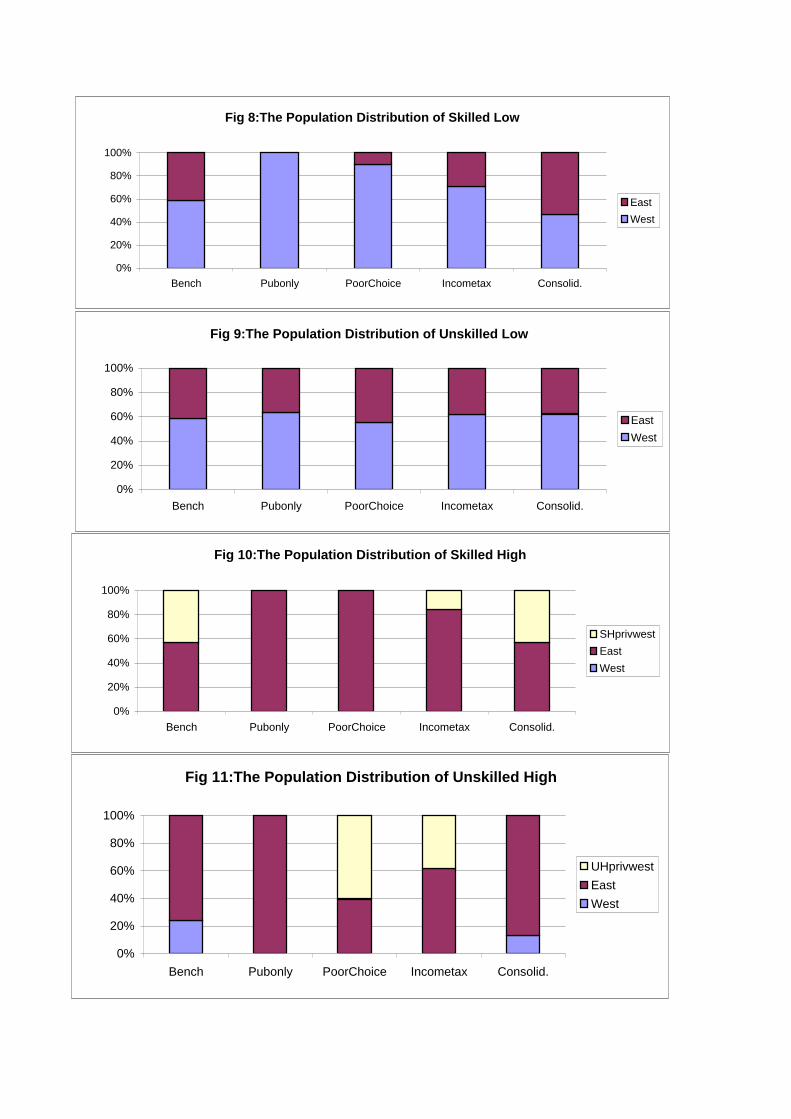
Fig 8:The Population Distribution of Skilled Low

0%

20%

40%

60%

80%

100%

Bench Pubonly PoorChoice Incometax Consolid.

EastWest

Fig 10:The Population Distribution of Skilled High

0%

20%

40%

60%

80%

100%

Bench Pubonly PoorChoice Incometax Consolid.

SHprivwestEastWest

Fig 9:The Population Distribution of Unskilled Low

0%

20%

40%

60%

80%

100%

Bench Pubonly PoorChoice Incometax Consolid.

EastWest

Fig 11:The Population Distribution of Unskilled High

0%

20%

40%

60%

80%

100%

Bench Pubonly PoorChoice Incometax Consolid.

UHprivwestEastWest