Embed Size (px)
Citation preview

School of Earth and Environment
Institute of Geophysics and Tectonics
Robust corrections for topographically-correlated atmospheric noise in InSAR data from large deforming regions
By David Bekaert
Andy Hooper, Tim Wright and Richard Walters

School of Earth and Environment Why a tropospheric correction for InSAR?
Tectonic
Over 9 months
100 km
cm
-10 13.5
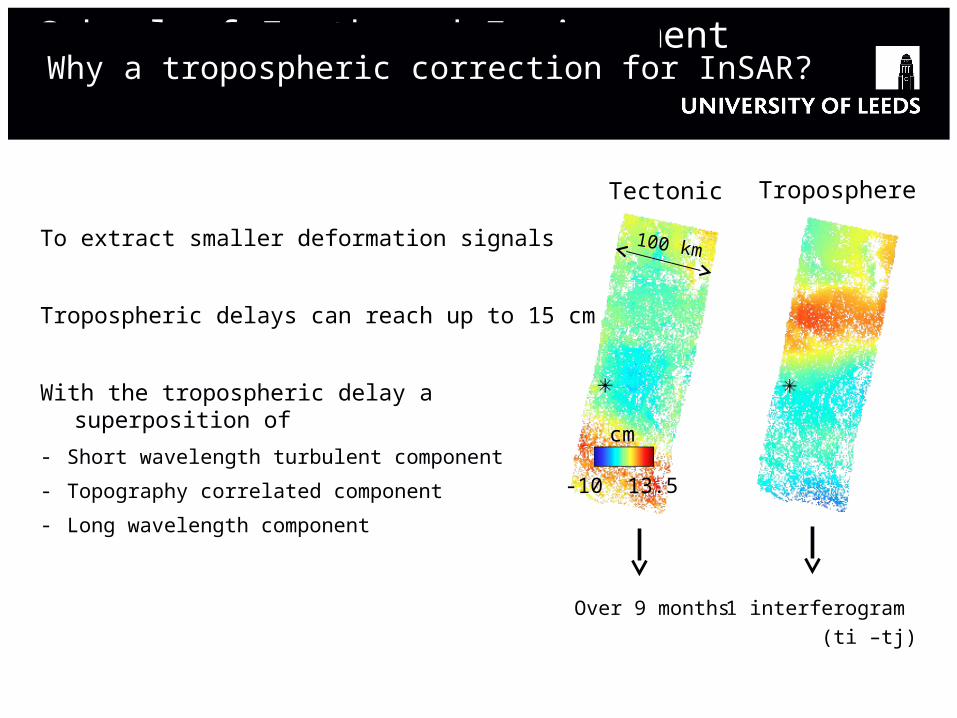
To extract smaller deformation signals
School of Earth and Environment
To extract smaller deformation signals
Tropospheric delays can reach up to 15 cm
With the tropospheric delay a superposition of
- Short wavelength turbulent component
- Topography correlated component
- Long wavelength component
Troposphere
1 interferogram
(ti –tj)
Tectonic
Over 9 months
100 km
cm
-10 13.5
Why a tropospheric correction for InSAR?

School of Earth and Environment
Auxiliary information (e.g.): Limitations
• GPS
• Weather models
• Spectrometer data
Station distribution
Accuracy and resolution
Cloud cover and temporal sampling
Tropospheric corrections for an interferogram

School of Earth and Environment
Auxiliary information (e.g.): Limitations
• GPS
• Weather models
• Spectrometer data
Interferometric phase
• Linear estimation (non-deforming region or band filtering)
Station distribution
Accuracy and resolution
Cloud cover and temporal sampling
Assumes a laterally uniform troposphere
isolines
€
Δφtropo =Kuniform ⋅ h +Const
Tropospheric corrections for an interferogram

School of Earth and Environment
A linear correction can work in small regions Interferogram
Tropo
GPS
InSAR and GPS data property of IGN
Linear est
isolines
€
Δφtropo =Kuniform ⋅ h +Const
A laterally uniform troposphere

School of Earth and Environment
However
• Spatial variation of troposphere
est: Spectrometer & Linear
isolines
+ +
- +
A linear correction can work in small regions
€
Δφtropo =Kuniform ⋅ h +Const
A spatially varying troposphere
Topography

School of Earth and Environment
Allowing for spatial variation
Interferogram (Δɸ)Why not estimate a linear function locally?
€
Δφtropo =Kuniform ⋅ h +Const
-9.75 rad 9.97A spatially varying troposphere

School of Earth and Environment
€
Δφtropo =Kuniform ⋅ h +Const
-9.75 rad 9.97A spatially varying troposphere
Why not estimate a linear function locally?
Does not work as:
Const is also spatially-varying and
cannot be estimated from original phase!
Interferogram (Δɸ)

School of Earth and Environment
€
Δφtropo =Kspatial ⋅ h0 − h( )α
€
Δφtropo =Kuniform ⋅ h +Const
-9.75 rad 9.97
We propose a power-law relationship
that can be estimated locally
A spatially varying troposphere
Why not estimate a linear function locally?
Does not work as:
Const is also spatially-varying and
cannot be estimated from original phase!
Interferogram (Δɸ)

School of Earth and Environment
€
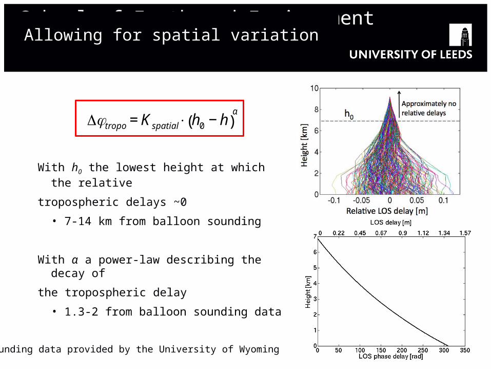
Δφtropo =Kspatial ⋅ h0 − h( )α
With h0 the lowest height at which the relative
tropospheric delays ~0
• 7-14 km from balloon sounding
Sounding data provided by the University of Wyoming
Allowing for spatial variation
School of Earth and Environment
Allowing for spatial variation
€
Δφtropo =Kspatial ⋅ h0 − h( )α
With h0 the lowest height at which the relative
tropospheric delays ~0
• 7-14 km from balloon sounding
With α a power-law describing the decay of
the tropospheric delay
• 1.3-2 from balloon sounding data
Allowing for spatial variation
Sounding data provided by the University of Wyoming

School of Earth and Environment Power-law example
€
Δφ =Kspatial ⋅ h0 − h( )α+ Δφdefo + ...
-9.75 rad 9.97
Interferogram (Δɸ)
School of Earth and Environment Power-law example
-9.75 rad 9.97
€
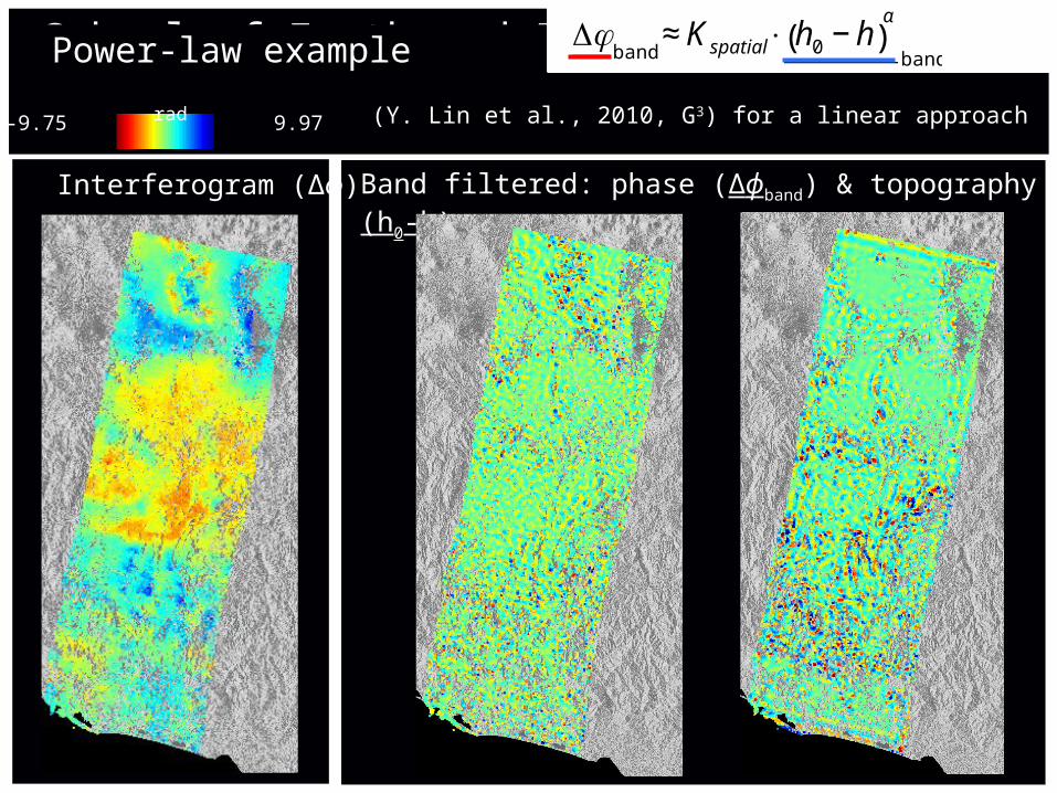
Δφband≈ Kspatial ⋅ h0 − h( )
α
band
Band filtered: phase (Δɸband) & topography (h0-h)αband
(Y. Lin et al., 2010, G3) for a linear approach
Interferogram (Δɸ)

School of Earth and Environment Power-law example
€
Δφband≈ Kspatial ⋅ h0 − h( )
α
band
Band filtered: phase (Δɸband) & topography (h0-h)αband
(Y. Lin et al., 2010, G3) for a linear approach

School of Earth and Environment Power-law example
Band filtered: phase (Δɸband) & topography (h0-h)αband €
Δφband≈ Kspatial ⋅ h0 − h( )
α
band
For each window:estimate Kspatial
(Y. Lin et al., 2010, G3) for a linear approach
Anti-correlated!

School of Earth and Environment Power-law example
€
Δφband≈ Kspatial ⋅ h0 − h( )
α
band
Band filtered: phase (Δɸband) & topography (h0-h)αband
For each window:estimate Kspatial
(Y. Lin et al., 2010, G3) for a linear approach
Anti-correlated!

School of Earth and Environment
Original phase (Δɸ)
Power-law example
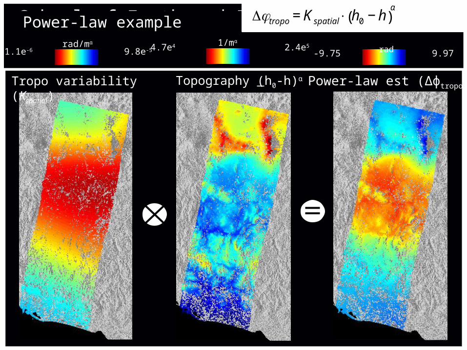
Band filtered: phase (Δɸband) & topography (h0-h)αband Tropo variability (Kspatial) €
Δφband≈ Kspatial ⋅ h0 − h( )
α
band
rad/mα -1.1e-6 9.8e-5
School of Earth and Environment
Original phase (Δɸ)
Power-law example
Band filtered: phase (Δɸband) & topography (h-h0)αband Tropo variability (Kspatial) €
Δφtropo =Kspatial ⋅ h0 − h( )α
Topography (h0-h)α
-1.1e-6 9.8e-5rad/mα
-9.75 rad 9.97
Power-law est (Δɸtropo)
4.7e4 2.4e51/mα
School of Earth and Environment
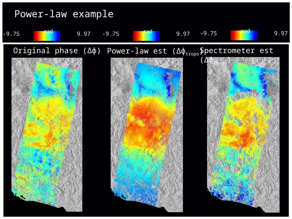
Allowing for spatial variation-9.75 rad 9.97 -9.75 rad 9.97 -9.75 rad 9.97
Original phase (Δɸ) Power-law est (Δɸtropo) Spectrometer est (Δɸtropo)
Power-law example

School of Earth and Environment
Regions:
• El Hierro (Canary Island)
- GPS
- Weather model
- Uniform correction
- Non-uniform correction
• Guerrero (Mexico)
- MERIS spectrometer
- Weather model
- Uniform correction
- Non-uniform correction
Case study regions

School of Earth and Environment
-11.2 rad 10.7
Interferograms(original)
El Hierro

School of Earth and Environment
WRF(weather model)
El Hierro
-11.2 rad 10.7
Interferograms(original)

School of Earth and Environment
WRF(weather model)
El Hierro
-11.2 rad 10.7
Interferograms(original)

School of Earth and Environment
WRF(weather model)
Linear(uniform)
El Hierro
-11.2 rad 10.7
Interferograms(original)

School of Earth and Environment
WRF (weather model)
Linear(uniform)
Power-law(spatial var)
El Hierro
-11.2 rad 10.7
Interferograms(original)

School of Earth and Environment El Hierro quantification
ERA-I run at 75 km resolution WRF run at 3 km resolution
School of Earth and Environment
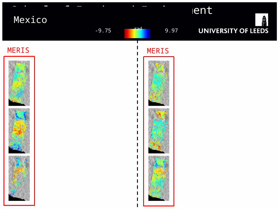
MERIS MERIS
Mexico-9.75 rad 9.97

School of Earth and Environment
MERIS MERIS
Clouds
Mexico-9.75 rad 9.97

School of Earth and Environment
MERIS ERA-I MERIS ERA-I
Mexico-9.75 rad 9.97(Weather model)

School of Earth and Environment
MERIS ERA-I MERIS ERA-I
Misfit near coast
Mexico-9.75 rad 9.97(Weather model)

School of Earth and Environment
MERIS ERA-I Linear MERIS ERA-I Linear
Mexico-9.75 rad 9.97(Weather model)
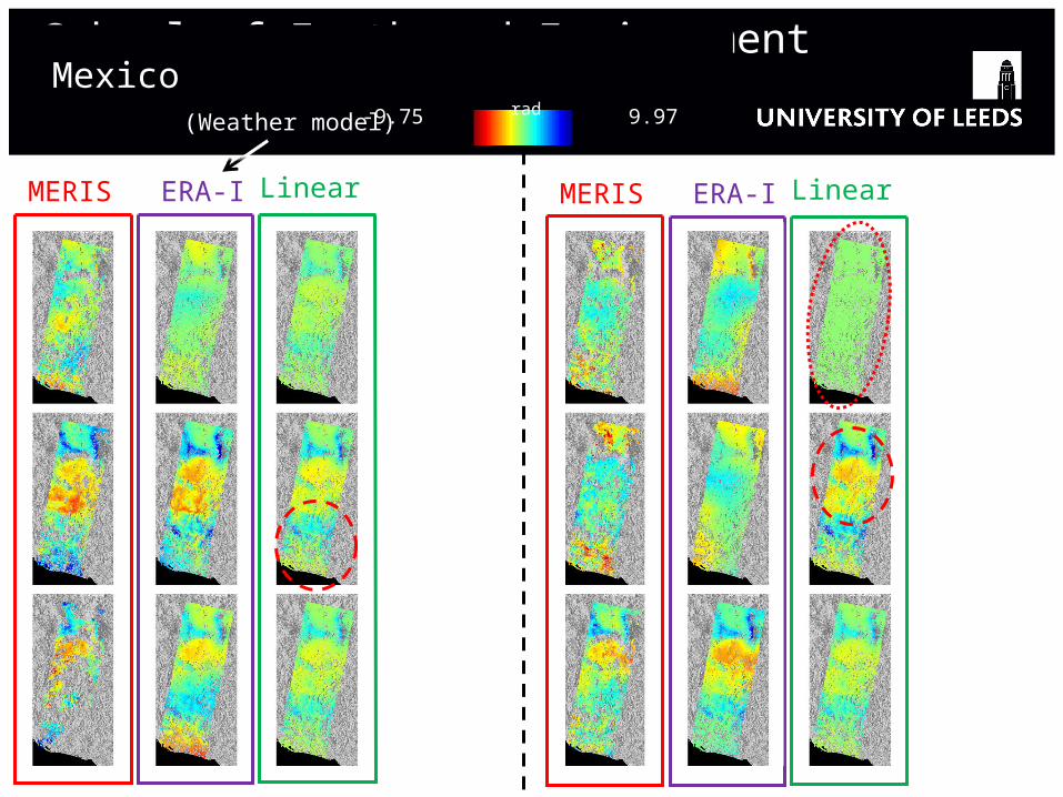
School of Earth and Environment
MERIS ERA-I Linear MERIS ERA-I Linear
Mexico-9.75 rad 9.97(Weather model)
School of Earth and Environment
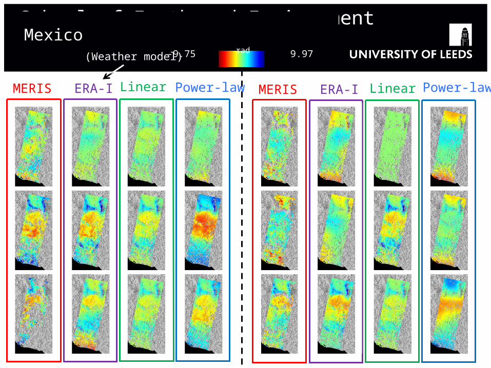
MERIS ERA-I Linear Power-law MERIS ERA-I Linear Power-law
Mexico-9.75 rad 9.97(Weather model)
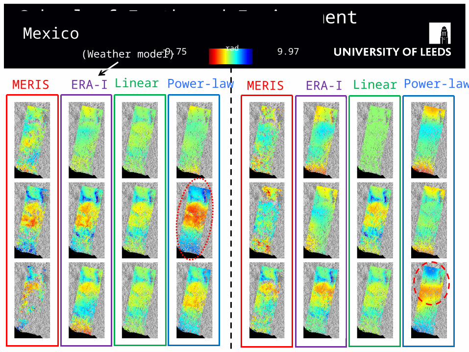
School of Earth and Environment
MERIS ERA-I Linear Power-law MERIS ERA-I Linear Power-law
Mexico-9.75 rad 9.97(Weather model)

School of Earth and Environment
MERIS ERA-I
Linear Power-law
Mexico techniques compared: profile AA’

School of Earth and Environment
MERIS accuracy
(Z. Li et al., 2006)
Mexico quantification
School of Earth and Environment
• Fixing a reference at the ‘relative’ top of the troposphere allows us to deal with spatially-varying tropospheric delays.
• Band filtering can be used to separate tectonic and tropospheric components of the delay in a single interferogram
• A simple power-law relationship does a reasonable job of modelling the topographically-correlated part of the tropospheric delay.
• Results compare well with weather models, GPS and spectrometer correction methods.
• Unlike a linear correction, it is capable of capturing long-wavelength spatial variation of the troposphere.
Summary/Conclusions
Toolbox with presented techniques will be made available to the community