School of Economics and FinanceA New Predictor of Real Economic Activity:

Working Paper No. 741 March 2015 ISSN 1473-0278

Sylvia Sarantopoulou-Chiourea and George Skiadopoulos

The S&P 500 Option Implied Risk Aversion

A New Predictor of Real Economic Activity: The S&P 500 Option

Implied Risk Aversion*

Sylvia Sarantopoulou-Chioureaa and George Skiadopoulosb

This draft: 17 March 2015

Abstract

We propose a new predictor of real economic activity (REA), namely the representative investor's

implied relative risk aversion (IRRA) extracted from S&P 500 option prices. IRRA exploits the

forward-looking information in option prices. It increases as risk averse investors enter the market,

leading to a decrease in market risk premium thus predicting a REA improvement. In line with our

hypothesis, IRRA predicts U.S. REA even when we control for well-known REA predictors. Results

hold over both short and long horizons and regardless of the way we conduct inference. Moreover,

IRRA forecasts REA out-of-sample over the 2008-2009 great economic recession peak.

Keywords: Option prices, Risk aversion, Risk-neutral moments, Real Economic Activity.

JEL Classification: E44, G13, G17

* We would like to thank Michael Anthropelos, Peter Christoffersen, Charoula Daskalaki, Jin-Chuan Duan, Marcelo

Fernandes, Anastasios Kagkadis, Eirini Konstantinidi, Alexandros Kostakis, Loriano Mancini, Haroon Mumtaz, Michael

Neumann, Stavros Panageas, Katerina Panopoulou, George Skoulakis, Christos Stefanadis, John Tsoukalas, Dimitri

Vayanos, Andrea Vedolin, Costas Xiouros, Weiqi Zhang, and participants at the 2014 Multinational Finance Society

Symposium at Cyprus for many useful comments and discussions. Any remaining errors are our responsibility.

a Department of Banking and Financial Management, University of Piraeus, Greece, e-mail: ssarant@unipi.gr

b Corresponding author. School of Economics and Finance, Queen Mary, University of London and Department of

Banking and Financial Management, University of Piraeus, Greece. Also Associate Research Fellow with Cass Business

School, City University London, and Warwick Business School, University of Warwick, UK,

g.skiadopoulos@qmul.ac.uk, gskiado@unipi.gr

1. Introduction

The question whether real economic activity (REA) can be predicted is of particular importance to

policy makers, firms and investors. Monetary and fiscal policy as well as the firms’ business plans

and investors' decisions are based on forecasts of REA. There is an extensive literature which studies

whether REA can be predicted by employing a number of financial variables (for a review, see Stock

and Watson, 2003). This literature has become even more topical recently when the 2007 turbulence

in the financial markets was followed by a significant economic recession which caught investors

and academics by surprise (Gourinchas and Obstfeld, 2012). These facts highlight the link between

financial markets and the real economy as well as the need to develop new accurate REA predictors

based on financial markets’ information.

In this paper, we explore whether the cross-section of index option market prices conveys

information for future REA. To this end, we propose a new predictor of REA. We investigate

whether the representative investor’s relative risk aversion (RRA) extracted from the S&P 500

market option prices (implied RRA, IRRA) predicts U.S. REA. The motivation for the choice of

our predictor is threefold. First, S&P 500 options are inherently REA forward-looking contracts.

Their payoff depends on the future state of the economy because the underlying stock index is a

broad one that eliminates idiosyncratic risk. Hence, option prices are expected to be superior REA

predictors to other financial variables for which their relation with future REA may not be clear and

their predictive ability has been questioned empirically.1 In addition, evidence suggests that

informed traders tend to prefer option markets rather than the underlying spot market to exploit their

informational advantage (e.g., Easley et al., 1998, Pan and Poteshman, 2006, and references therein)

thus making option-based measures even more appealing for forecasting REA. Second, IRRA

1 For instance, stock variables have also been claimed to be forward-looking instruments based on the rationale that their

values depend on future cash flows (i.e. dividends). However, the correlation between dividends and REA is weak

(Subrahmanyam and Titman, 2013).

2

synopsizes the information in market index option prices trading across the spectrum of strikes by

construction. Third, from an asset pricing perspective, RRA determines discount rates which are

related to future REA (Fama, 1990, Cochrane, 2011). Therefore, it is appealing to summarize the

options’ information in a RRA measure.

We extract a time series of IRRA values using Kang et al. (2010) formula which employs the

S&P 500 risk-neutral volatility, risk-neutral skewness, risk-neutral kurtosis and the physical variance

as inputs. We calculate the risk-neutral moments via the Bakshi et al. (2003) method which uses the

cross-section of traded S&P 500 option prices. Hence, IRRA incorporates information from all

traded options by construction. Our estimated IRRA values are positive and their magnitude is

plausible and within the range of values reported by previous literature. In addition, IRRA is

positively correlated with the S&P 500.

Next, we investigate whether IRRA forecasts future REA. To this end, we use three

alternative measures to proxy REA: industrial production, nonfarm private payroll employment and

the Kansas financial stress index. We test IRRA’s forecasting ability across different forecasting

horizons up to one year both in a stand-alone setting as well as jointly with a large set of variables

documented by the previous literature to predict REA. This set comprises the “traditional” interest

rate spreads (default, term and TED spreads) and equity asset pricing factors as well as the more

recently documented REA predictors such as the forward variances inferred from option prices,

variance risk premium, Baltic dry index, commodity open interest and commodity-specific factors.

We conduct statistical inference carefully by coping with small sample biases, overlapping

observations and persistence of regressors.

We find that an increase (decrease) in IRRA predicts an increase (decrease) in REA. Most

importantly, we find that IRRA predicts future REA over and above these predictors regardless of

the REA measure. Therefore, IRRA contains information that has not already been incorporated by

other financial predictors. Depending on the REA proxy, the addition of our proposed predictor

3

increases the adjusted R2 by 20% to 65% relative to a model which uses only the predictors proposed

by the previous literature. The adjusted R2 increases (decreases) with the forecasting horizon when

REA is measured by the industrial production index (nonfarm private payroll employment and the

Kansas financial stress index). These results are robust and they hold regardless of the way we

conduct statistical inference. In addition, within an out-of-sample setting, IRRA predicts REA more

accurately than other financial predictors do over the 2008-2009 peak of the recent financial crisis

and the subsequent great economic recession. Finally, we explore the origin of the statistical

significance of IRRA by attributing it to its inputs. We find that IRRA’s forecasting ability stems

from the option information based inputs used to estimate it, and more specifically from the risk-

neutral moments of the S&P 500 distribution.

The fact that an increase (decrease) in IRRA predicts an increase (decrease) in REA can be

explained as follows. Wilson (1968, Theorems 4 and 5) and Hara et al. (2007, Lemma 1) show that

the representative agent’s RRA is a weighted average of the individual agents RRAs. Notice that the

representative agent’s IRRA takes into consideration only the risk aversion of the individual agents

who participate in the stock market, thus ignoring the risk aversion of the non-market participants.

Therefore, in the case where investors expect an improvement (deterioration) in REA, the more risk

averse investors return (exit) to (from) the market and as a result IRRA increases (decreases). At the

same time, the stock market does well (badly) because of buying (selling) orders and as a result the

expected returns decrease (increase). This will lead to an improvement (deterioration) of REA.

Our explanation for the relation between IRRA and REA is consistent with our finding that

IRRA is positively correlated with the S&P 500. Barone-Adesi et al. (2014) and Duan and Zhang

(2014) also report a positive correlation between IRRA and the stock market. 2 This may seem to be

2 Barone-Adesi et al. (2014) offer an alternative behavioral finance explanation for the positive correlation between the

option implied RRA and the S&P 500. Prospect theory suggests that risk aversion will be lower after market losses than

after market gains.

4

a counterintuitive result at a first glance. Asset pricing theory suggests that an increase in RRA

increases expected return and so it should decrease the stock index price. However, the discussed

above relation between the representative agent’s and the individuals investors' RRAs as well as the

nature of IRRA estimates which is distinct from that of RRA estimated via standard consumption

asset pricing models explains this seemingly counterintuitive result. The RRA estimated from

standard consumption asset pricing models does not confine itself only to stock market investors.

Hence, it does not depend only on investors’ entry-exit behavior in the stock market and as a result

its time series behavior differs from IRRA’s. Typically, it is reported to be countercyclical (e.g.,

Campbell and Cochrane, 1999, Xiouros and Zapatero, 2010). We verify the IRRA dependence on

individual investor’s entry/exit in the stock market by documenting a positive relation between IRRA

and U.S. equity mutual funds net flows. The latter reflect individual investors’ risk attitudes because

they are determined primarily by individual investors. In 2013, U.S. households held 90 percent of

total mutual fund assets (Investment Company Institute, 2014).

As a by-product of our analysis, we also find that commonly perceived measures of risk

aversion such as VIX, the variance risk premium, put/call ratio and risk-neutral skewness are not

correlated with IRRA. This is not surprising though. Some of the previously proposed variables to

proxy risk aversion are expected to do so only under strong modeling assumptions (Bollerslev et al.,

2011) and some others are based on intuition thus rendering the use of these variables as a proxy of

the unobservable RRA questionable (Coudert and Gex, 2008).

Related literature: Our paper ties three strands of literature. The first strand has to do with

the use of financial variables to predict REA. The rationale is that financial markets reflect investors’

perceptions about the future state of the economy and hence they can predict REA. The term spread

(Estrella and Hardouvelis, 1991) and default spread (Stock and Watson, 2003) are two prominent

predictors of REA. An increase (decrease) in the term spread predicts an expansion (recession) of

REA whereas an increase in the default spread signifies a recession. More recently, other financial

5

variables such as asset pricing factors (Liew and Vassalou, 2000), the TED spread (Chiu, 2010),

forward variances inferred from options (Bakshi et al., 2011), the Baltic dry index (Bakshi et al.,

2012), commodity futures open interest (Hong and Yogo, 2012), and commodity-specific factors

(Bakshi et al., 2014) have been found to predict REA.

The second strand of literature has to do with the estimation of the representative agent's risk

aversion from index options market prices. This is possible due to the theoretical relation of risk

aversion to the ratio of the risk-neutral distribution and the subjective distribution of the option's

underlying index; the former can be recovered from option prices (for a review, see Jackwerth,

2000). Ait-Sahalia and Lo (2000) Jackwerth (2000), Bliss and Panigirtzoglou (2004) and Kang and

Kim (2006) obtain single IRRA estimates. Rosenberg and Engle (2002), Bakshi and Madan (2006),

Kang et al. (2010), Kostakis et al., (2011), Barone-Adesi et al., (2014) and Duan and Zhang (2014)

estimate a time series of IRRA. We choose the Kang et al., (2010) methodology to estimate IRRA

because it is parsimonious in terms of the required inputs. Most importantly, these inputs can be

estimated accurately from the cross-section of market option prices which are readily available.

The third strand of literature uses the informational content of market option prices to address

a number of topics in economics and finance. The rationale is that market option prices convey

information which can be used for policy making (Söderlind and Svensson, 1997), risk management

(Chang et al., 2012, Buss and Vilkov, 2012), asset allocation (Kostakis et al., 2011, DeMiguel et al.,

2013) and stock selection purposes (for reviews, see Chang et al., 2012, Giamouridis and

Skiadopoulos, 2012). Surprisingly, there is a paucity of research on whether the information

embedded in index option prices can be used to predict REA, too. To the best of our knowledge,

6

Bakshi et al. (2011) is the only paper which explores this and it documents that forward variances

extracted from index options forecast REA.3

The rest of the paper is structured as follows. Section 2 describes the data and Section 3

explains IRRA’s estimation, required inputs and results on its time variation. Section 4 presents the

testable hypothesis and evidence on the IRRA as a predictor of REA. Section 5 verifies that IRRA’s

predictive ability stems from option prices informational content. Section 6 concludes.

2. Data and key variables

For the purposes of our analysis, we use monthly (end-of-month) data.

2.1 Options data

We obtain S&P 500 European style index option data (quotes prices) for the period January 1996 to

December 2012 from the Ivy DB database of OptionMetrics. We use the S&P 500 implied

volatilities provided by Ivy DB for each traded contract. These are calculated based on the midpoint

of bid and ask prices using Merton's (1973) model. In addition, we obtain the closing price of the

S&P 500 and the continuously paid dividend yield from Ivy DB. We filter the options data to remove

any noise. We only consider out-of-the-money and at-the-money options with time-to-maturity 5 to

270 days. We also discard options with zero open interest and zero trading volume. Furthermore,

we retain only option contracts that do not violate Merton's, 1973, no-arbitrage condition and have

implied volatilities less than 100%. We also eliminate options that form vertical and butterfly

spreads with negative prices and option contracts with zero bid prices and premiums. As a proxy

for the risk-free rate, we use the continuously compounded U.S. LIBOR rates with maturities one to

3 Bali et al. (2012) find that a measure of the stock market riskiness constructed from individual equity options predicts

future economic downturns. Neumann (2014) finds that the prices of options written on bank stocks predict future REA.

In the context of bond markets, Mueller et al. (2013) find that the variance risk premium extracted from bond option

prices also forecasts REA.

7

six months taken from Bloomberg. To obtain the rate for any other required maturity, we use linear

interpolation across the closest available maturities. In addition, we obtain the history of expected

dividend payments over the life of each option contract and their timing provided by IvyDB. These

expected dividend payments have been calculated based on the assumption of constant dividend

yields over the life of the option.

Finally, we construct two measures of the forward variances inferred from option prices, in

accordance with Bakshi et al. (2011). We construct at time t the forward variance FVt1(30) between

t and t+30 and the forward variance FVt2(30) between t+30 and t+60. Appendix A describes the

calculation of the forward variances from the market prices of call and put option portfolios.

2.2 Other variables

We collect data on a number of variables for the period July 2002 to December 2012. We obtain the

net cash flows of all U.S. equity funds calculated as the difference of inflows minus the outflows

from Bloomberg. In addition, we obtain the VIX implied volatility index and the put/call ratio from

Bloomberg. We also obtain data on Moody’s BAA and AAA corporate bond spreads and the 3-

month and 10- year U.S. government treasury yields from the Federal Reserve Bank of St. Louis

(FRED) website to calculate the default and term spreads, respectively. We calculate the TED spread

as the difference between the 3-month U.S. LIBOR rate and the 3-month U.S. Treasury Bill.

Furthermore, we obtain the monthly Fama-French (1996) high minus low (HML) and small minus

big (SMB) factors from Kenneth R. French's website.

We also obtain data on 22 individual commodity futures from Bloomberg and we construct

the three Daskalaki et al. (2014) commodity-specific factors (hedging-pressure, momentum and

basis factors); Appendix B provides a detailed description of the construction of these factors. Table

1 lists the employed commodities categorized in five sectors (grains and oilseeds, energy, livestock,

metals and softs). In addition, we construct a commodity futures open interest variable following

8

the approach of Hong and Yogo (2012). First, we compute the growth rate of open interest for each

commodity futures. Then, we compute the median of the growth rates of open interest for all

commodities futures of each sector. Last, we compute the equally weighted average of the medians

growth rates of all sectors.

We proxy REA by three alternative measures. We use the non-farm payroll (Payroll) in line

with Beber and Brandt (2006) and Bakshi et al. (2011). We also follow Allen et al. (2012) and

Neumann (2014) and we use the industrial production (IPI) growth rate and the Kansas City

Financial Stress Index (KCFSI). IPI measures the amount of the industries output. Nonfarm payroll

is an indicator of the state of the labour market. KCFSI measures the financial stress in the U.S.

economy. A positive value indicates that financial stress is above the long-run average, while a

negative value signifies that financial stress is below the long-run average. KCFSI is associated with

REA through three channels (Hakkio and Keeton, 2009). First, an increase in financial stress

increases the uncertainty about the asset prices, agents reduce their spending, and thus REA

decreases. Second, it increases the agents’ cost of financing spending which leads again to a decrease

in REA. Third, it decreases the lending opportunities, as a result REA decreases too. The IPI and

non-farm-payroll time series are seasonally adjusted obtained from the FRED website. KCFSI is

downloaded from the Federal Reserve Bank of Kansas City website. We collect data for all three

proxies for the period July 2002 to November 2013.

Finally, we obtain daily realized variances from the Realized Library of the Oxford-Man

Institute of Quantitative Finance. Realized variances are the sum of intra-day squared 5-minute

returns within each day and they are available for the period January 2000- December 2012.

9

3. Extraction of risk aversion from option prices

3.1 Formula and estimation method

Assuming that the representative agent’s preferences are described by a power utility function,

Bakshi and Madan (2006) derive a formula which can be used to extract RRA from European options

market prices. Let be the coefficient of relative risk aversion, and 2 2, ,( ), ( )q t p t , , ( )p t and

, ( )p t denote the risk-neutral variance, physical variance, physical skewness and physical kurtosis

of the index continuously compounded returns distribution at time t with horizon , respectively.

Then,

2 2 21/2, , 2 2, , , ,2

,

( ) ( )( ) ( ) ( ) ( ) 3

( ) 2q t p t

p t p t p t p tp t

(1)

RRA can be estimated from equation (1). However, the RRA estimation requires estimation

of the higher order physical moments first. Their estimation is challenging. On the one hand, a long

time series is required to estimate them accurately. On the other hand, a small sample size is needed

to capture their time variation (Jackwerth and Rubinstein, 1996). To avoid the problem of estimating

the physical higher order moments, we resort to the Kang et al. (2010) formula which is a variant of

equation (1), i.e.

2 2 21/2, , 2 2, , , ,2

,

( ) ( )( ) ( ) ( ) ( ) 3

( ) 2p t q t

q t q t q t q tq t

(2)

where , ( )q t and , ( )q t is the skewness and kurtosis, respectively, of the risk-neutral index

distribution at time t with horizon . Kang et al. (2010) derive equation (2) by also assuming that

the representative agent’s preferences are described by a power utility function. Then, they use the

10

moment generating functions of the risk-neutral and physical probability distributions and they

truncate their expansion series appropriately.

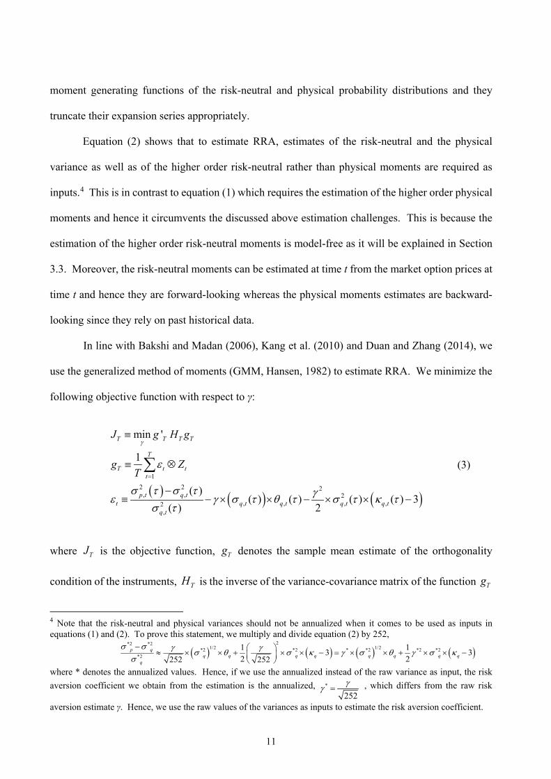
Equation (2) shows that to estimate RRA, estimates of the risk-neutral and the physical

variance as well as of the higher order risk-neutral rather than physical moments are required as

inputs.4 This is in contrast to equation (1) which requires the estimation of the higher order physical

moments and hence it circumvents the discussed above estimation challenges. This is because the

estimation of the higher order risk-neutral moments is model-free as it will be explained in Section

3.3. Moreover, the risk-neutral moments can be estimated at time t from the market option prices at

time t and hence they are forward-looking whereas the physical moments estimates are backward-

looking since they rely on past historical data.

In line with Bakshi and Madan (2006), Kang et al. (2010) and Duan and Zhang (2014), we

use the generalized method of moments (GMM, Hansen, 1982) to estimate RRA. We minimize the

following objective function with respect to :

12 2 2

, , 2, , , ,2

,

min '

1

( )( ) ( ) ( ) ( ) 3

( ) 2

T T T T

T

T t tt

p t q tt q t q t q t q t

q t

J g H g

g ZT

(3)

where TJ is the objective function, Tg denotes the sample mean estimate of the orthogonality

condition of the instruments, TH is the inverse of the variance-covariance matrix of the function Tg

4 Note that the risk-neutral and physical variances should not be annualized when it comes to be used as inputs in equations (1) and (2). To prove this statement, we multiply and divide equation (2) by 252,

2*2 *2

1/2 1/2*2 *2 * *2 *2 *2*2

1 13 32 2252 252

p qq q q q q q q q

q

where * denotes the annualized values. Hence, if we use the annualized instead of the raw variance as input, the risk aversion coefficient we obtain from the estimation is the annualized, *

252, which differs from the raw risk

aversion estimate . Hence, we use the raw values of the variances as inputs to estimate the risk aversion coefficient.

11

and TZ are the instruments. In equation (3), there are as many moment conditions as instruments.

In line with Bakshi and Madan (2006), Kang et al. (2010) and Duan and Zhang (2014), we use three

different sets of instruments for robustness. The first set consists of a constant and one lag of the

risk-neutral variance 2, 1( )q t . The second set consists of a constant and two lags of the risk-neutral

variance [ 2, 1( )q t , 2

, 2 ( )q t ]. The third set contains a constant and three lags of the risk-neutral

variance [ 2, 1( )q t , 2

, 2 ( )q t , 2, 3 ( )q t ]. We extract RRA for a constant time horizon =30 days.

All three studies document that the moment restrictions imposed by equation (3) are not rejected by

the data for the S&P 100 and S&P 500 markets for any given set of instruments.

3.2 Inputs estimation

We extract the S&P 500 risk-neutral moments from market option prices following the Bakshi et al.

(2003) methodology. The advantage of this methodology is that it is model-free because it does not

require any specific assumptions for the underlying’s asset price stochastic process.

Let S(t) be the price of the underlying asset at time t, r the risk-free rate and

( , ) ln lnR t S t S t the -period continuously compounded return. The computed at

time t model-free risk-neutral volatility (IV), skewness (SKEW) and kurtosis (KURT) of the log-

returns ( , )R t distribution with horizon are given by:

Q 2 2 r 2tIV( t , ) E R( t , ) ( t , ) V( t , )e ( t , ) (4)

Q Q 3t t

3Q Q 2 2t t

r r 3

3r 2 2

E ( R( t , ) E R( t , ) )SKEW( t, )

E ( R( t , ) E R( t , ) )

e W( t , ) 3 ( t , )e V( t , ) 2 ( t , )

e V( t , ) ( t , )

(5)

12

Q Q 4t t

2Q Q 2t t

r r r 2 4

2r 2

E ( R( t , ) E R( t , ) )KURT( t , )

E ( R( t , ) E R( t , ) )

e X( t , ) 4 ( t , )e W( t , ) 6e ( t , ) V( t , ) 3 ( t , )

e V( t , ) ( t , )

(6)

where V(t, ), W(t, ) and X(t, ) are the fair values of three artificial contracts (volatility, cubic and

quartic contract) defined as:

2 3 4( , ) ( , ) , ( , ) ( , ) , ( , ) ( , )Q r Q r Q rt t tV t E e R t W t E e R t X t E e R t (7)

and (t, ) is the mean of the log return for period defined as:

r r rQ rt

S( t ) e e e( t , ) E ln e 1 V( t , ) W( t , ) X ( t , )S( t ) 2 6 24

(8)

The prices of the three contracts can be computed as a linear combination of out-of-the-money call

and put options:

S( t )

2 2S( t ) 0

K S( t )2 1 ln 2 1 lnS( t ) KV( t , ) C t , ;K dK P t, ;K dK

K K(9)

2 2

S( t )

2 2S( t ) 0

K K S( t ) S( t )6 ln 3 ln 6 ln 3 lnS( t ) S( t ) K KW( t, ) C t , ;K dK P t, ;K dK

K K(10)

2 3

2S( t )

2 3

S( t )

20

K K12 ln 4 lnS( t ) S( t )

X ( t , ) C t , ;K dKK

S( t ) S( t )12 ln 4 lnK K P t, ;K dK

K

(11)

13

where C( t , ;K )( P( t , ;K ) ) are the call and put prices with strike price and time to maturity .

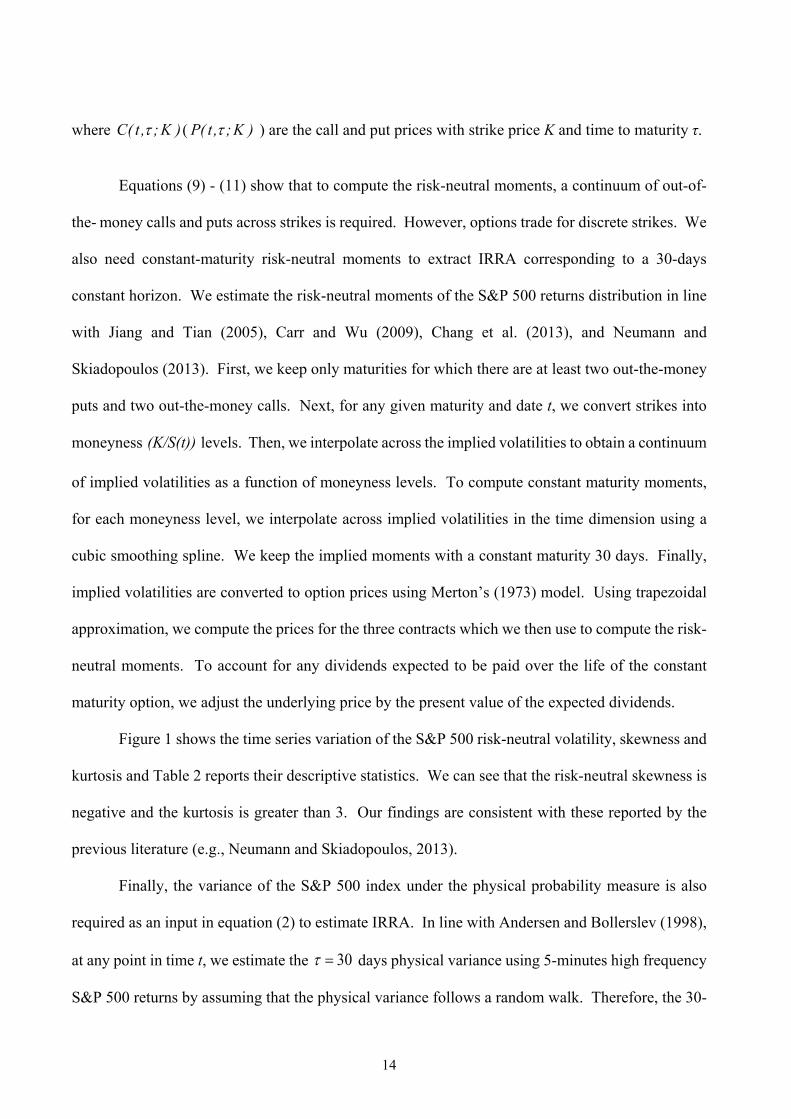
Equations (9) - (11) show that to compute the risk-neutral moments, a continuum of out-of-

the- money calls and puts across strikes is required. However, options trade for discrete strikes. We

also need constant-maturity risk-neutral moments to extract IRRA corresponding to a 30-days

constant horizon. We estimate the risk-neutral moments of the S&P 500 returns distribution in line

with Jiang and Tian (2005), Carr and Wu (2009), Chang et al. (2013), and Neumann and

Skiadopoulos (2013). First, we keep only maturities for which there are at least two out-the-money

puts and two out-the-money calls. Next, for any given maturity and date t, we convert strikes into

moneyness (K/S(t)) levels. Then, we interpolate across the implied volatilities to obtain a continuum

of implied volatilities as a function of moneyness levels. To compute constant maturity moments,

for each moneyness level, we interpolate across implied volatilities in the time dimension using a

cubic smoothing spline. We keep the implied moments with a constant maturity 30 days. Finally,

implied volatilities are converted to option prices using Merton’s (1973) model. Using trapezoidal

approximation, we compute the prices for the three contracts which we then use to compute the risk-

neutral moments. To account for any dividends expected to be paid over the life of the constant

maturity option, we adjust the underlying price by the present value of the expected dividends.

Figure 1 shows the time series variation of the S&P 500 risk-neutral volatility, skewness and

kurtosis and Table 2 reports their descriptive statistics. We can see that the risk-neutral skewness is

negative and the kurtosis is greater than 3. Our findings are consistent with these reported by the

previous literature (e.g., Neumann and Skiadopoulos, 2013).

Finally, the variance of the S&P 500 index under the physical probability measure is also

required as an input in equation (2) to estimate IRRA. In line with Andersen and Bollerslev (1998),

at any point in time t, we estimate the 30 days physical variance using 5-minutes high frequency

S&P 500 returns by assuming that the physical variance follows a random walk. Therefore, the 30-

14

calendar-days physical variance 2, ( )p t equals the realized variance ,t tRV computed as the sum of

the daily realized variances and the sum of the overnight squared returns (OR ) of the S&P 500 over

the last 30 days:

2 2,

t t

t t i ii t i t

RV OR (12)

Daily realized variances are obtained from the Realized Library of the Oxford-Man Institute of

Quantitative Finance. Overnight returns are calculated as the log difference of each day’s opening

price minus the closing price of the previous day: 1ln lnOp Clt tOR S S , where ,Op ClS S are the

opening and the closing prices of the index, respectively.

3.3 IRRA: Results

We record the risk-neutral moments and the realized variance at the last trading day of each month

and we use equation (2) to estimate the monthly IRRA series with a rolling GMM estimation using

a rolling window of size 30 months.5 As a result, we extract the IRRA series for the period July

2002 - December 2012 given that our option dataset spans the period January 1996 to December

2012.

We use three different sets of instruments. Each set includes a constant and one to three lags

of the risk-neutral variance, respectively. First, we estimate IRRA over the full sample to check

whether its magnitude would be in line with the IRRA estimates provided by the previous literature.

We find that the full sample IRRA coefficient is 9.49, 8.84 and 8. 95 for the three respective sets of

instruments. These values fall within the range of IRRA values reported by the previous literature.

5 We have also estimated IRRA with rolling windows of sizes 45 and 60 months. The results are similar to the IRRA

estimated with a 30 months rolling window.

15

Ait-Sahalia and Lo (2000) report a full IRRA of 12.7, Rosenberg and Engle (2002) report values

from 2.26 to 12.55, Bakshi et al. (2003) report values between 1.76 and 11.39, Bliss and

Panigirtzoglou (2004) report a full sample estimate of 4.08, Bakshi and Madan (2006) report values

from 12.71 to 17.33, Kang and Kim (2006) report values between 2 and 4, Kang et al. (2010) 1.2 to

1.4, Barone-Adesi et al. (2014) report values between -0.5 and 3, and Duan and Zhang (2014) obtain

values from 1.8 to 7.1.

Regarding the monthly times series of IRRA extracted from the rolling GMM, Figure 2

shows IRRA’s time variation for each one of the three sets of instruments. The values are all positive

and they range between 1.71 to 12.15. Each one of IRRA’s time variation is similar across all three

sets of instruments. In the remainder of the paper, we report results for the case of the IRRA

estimated by the second set of instruments comprising the constant and two lags of the risk-neutral

variance.

Two remarks are in order regarding IRRA’s time series behavior. First, IRRA is quite

persistent. This is a feature that we will take into account in the statistical inference we will conduct

subsequently by means of bootstrapping estimators’ standard errors.6 Second, IRRA co-moves with

the S&P 500 (Figure 2). This implies that in periods when the S&P 500 rises (falls), risk aversion

rises (falls) too. Barone-Adesi et al. (2014) and Duan and Zhang (2014) also extract IRRA that are

positively correlated with the stock market. We will comment further on this IRRA’s property in

Section 4.1. In addition, IRRA is procyclical. Figure 3 shows the time variation of IRRA with the

three REA proxies. We can see that IRRA is positively correlated with the procyclical proxies of

REA (correlation of 0.30 and 0.70 with the growth rates of the industrial production index and the

6 Standard unit root tests indicate that IRRA is non-stationary. However, Cochrane (1999) shows that these tests cannot

distinguish between a stationary and a non-stationary series in finite samples. In addition, IRRA is expected to be

bounded from an economic theory perspective. Therefore, we do not difference IRRA to avoid discarding valuable

information and instead we take its persistence into account when conducting statistical inference.

16

nonfarm payroll employment, respectively) and negatively correlated with the countercyclical

Kansas City Financial Stress Index (KCFSI) (correlation of -0.74).

As a by-product of our analysis, IRRA can be used to test whether variables proposed by

the previous literature to proxy the representative agent's RRA actually do so. We consider four

such variables: VIX, the variance risk premium, put call ratio and risk-neutral skewness. VIX is

commonly considered as a measure of investor’s fear (Whaley, 2000). Bollerslev et al. (2011) and

Bekaert and Hoerova (2013) use VRP as a proxy of risk aversion. Finally, put call ratio is considered

to be a proxy for investor’s sentiment and risk-neutral skewness may proxy risk aversion (Bakshi et

al., 2003). To investigate whether these variables proxy risk aversion, we calculate the pairwise

correlations of the implied RRA with them (we use the variables in their first differences). We

measure VRP as the difference of the conditional expectations of the physical variance 2, [ ( )]p t tE

and that of the risk-neutral variance 2, [ ( )]q t tE .

2 2, ,VRP ( ) [ ( )] [ ( )]t p t t q t tE E (13)

We estimate the conditional expectation of the physical variance as the realized variance from time

t to . We measure the conditional expectation of the variance under the risk-neutral measure by

equating it to the squared VIX index (Jiang and Tian, 2007). We find that none of these variables is

highly correlated with the option implied RRA. The correlation of IRRA with VIX, VRP, put/call

ratio and risk-neutral skewness is -0.06, -0.06, -0.02 and -0.02, respectively. This shows that

commonly perceived measures of risk aversion are not correlated with the option implied RRA. This

is not surprising given that the above variables have been used by the previous literature as RRA

proxies based either on intuition (VIX, put/call ratio, risk-neutral skewness) or on specific modeling

assumptions (Bollerslev et al., 2011 assume that VRP is linear in volatility to establish the relation

between VRP and RRA).

17

4. Predicting REA

First, we formulate our testable hypothesis by explaining why we expect that IRRA would forecast

REA. Then, we test our hypothesis by examining whether IRRA predicts REA first over monthly

horizons and subsequently over longer horizons. We employ an in-sample setting and then an out-

of-sample one.

4.1 IRRA and REA: Testable hypothesis

We expect that an increase (decrease) in IRRA will lead to an increase (decrease) in REA. This

testable hypothesis stems from (a) the relation between the representative investor’s RRA and the

individual investors’ RRAs, and (b) the fact that IRRA takes into consideration only the risk aversion

of the individuals that participate in the market, ignoring the risk aversion of the non-market

participants. In particular, Wilson (Theorems 4 and 5, 1968) and Hara et al. (Lemma 1, 2007) show

that the representative agent's RRA is a weighted average of the individual agents' RRAs. Investors

decide whether to participate in the stock market, according to their degree of risk aversion and given

their expectations about the future state of the economy. In the case where stock investors expect an

improvement (deterioration) in REA, then IRRA will increase (decrease) because the more risk

averse investors will enter (exit) the market. As a result, the stock index price will increase

(decrease) because of buying (selling) orders and thus the equity premium will decrease (increase)

leading to an increase (decrease) in REA.

Our testable hypothesis is consistent with our finding in Section 3.3 where we document that

IRRA is positively correlated with the stock market. For instance, Duan and Zhang (2014) document

a high equity risk premium for the S&P 500 over the 2007-2009 subprime crisis where IRRA

decreases as the S&P 500 decreases. This would be expected to slow down REA. Indeed, this was

the case as experienced with the 2008-2009 great economic recession. Moreover, we test our

conjecture that market participants exit (participate in) the stock market in bad (good) times and this

18

decreases (increases) the representative agents' IRRA. To this end, we explore the relation of net

flows to U.S. equity mutual funds and the extracted IRRA. This relation should be positive under

our hypothesis. The representative agent’s IRRA should decrease (increase) when the more risk-

averse investors exit (return to) the market, i.e. when the net flows decrease (increase). We regard

mutual funds flows as an informative proxy of individual investors’ risk attitudes. The Investment

Company Institute (ICI, 2014) reports that 96 million individual U.S. investors or 46 percent of all

U.S. households owned mutual funds and held 90 percent of total mutual fund assets directly or

through retirement plans at year-end in 2013. Therefore, mutual funds flows are decided

predominantly by individual investors and hence they are expected to reflect their risk aversion to a

reasonable extent; this is not the case for the flows of other institutional investors.

Figure 4 shows the representative agent's IRRA and the net fund flows to U.S. equity mutual

funds time variation. We can see that IRRA co-moves with the equities net funds flows in most of

the sample period, i.e. in the case where IRRA is high, the net flows of the equity funds are also

high. Next, we regress IRRA on the net fund flows. Table 3 reports the results of the regression.

We can see that the funds flows coefficient is statistically significant and it has a positive sign, i.e.

an increase in funds net flows increases IRRA. This finding is in line with our argument that risk

aversion co-moves with the market because of the entry/exit of institutional investors in the market

depending on market conditions. In good (bad) times, investors become less (more) risk averse, i.e.

they enter (exit) the market by investing more (less) in equity funds and as a result IRRA increases

(decreases).

4.2 Single predictor models

To identify whether IRRA predicts REA over monthly horizons, first we regress each one of the

employed measures of REA on IRRA. For a start, we run single predictor regressions to investigate

the marginal effect of IRRA on each REA proxy, i.e.

19

, 1 1REA RRAi t t tc b (14)

where , 1i tREA denotes the i=1, 2, 3 proxies of real economic activity at t+1 (one month ahead) and

tRRA the IRRA at t.

The sample spans the period August 2002- December 2012. This yields 125 observations.

To address the potential presence of small sample bias on the statistical inference of the obtained

results, we report both Newey-West (1994) p-values as well as bootstrapped p-values. We calculate

the latter by implementing a stationary bootstrap estimation by modifying Politis and Romano (1994)

method. We introduce the modification to correct for the Stambaugh (1999) bias. This arises

because we perform predictive regressions on a lagged stochastic variable which is a persistent

regressor and as a result any bias in the autocorrelation coefficient will map to a bias in the beta

coefficient; we test and we find that the IRRA regressor follows an autoregressive process of order

one (AR(1)). Appendix C provides a detailed description of the bootstrap methodology.

Column (1) in Tables 4, 5, 6 reports the results from the single predictor OLS predictive

regressions using the respective three REA proxies. The forecasting horizon is one month. The

coefficient estimates, Newey-West (1994) p-values estimated with a Bartlett kernel and a lag in the

autocorrelation process for the error term (ARMA(p, q)) (Newey-West, 1994, Theorem 1), the two-

sided p-values obtained from the stationary bootstrap (within parenthesis) and the adjusted R2 for

each REA proxy are reported.

We can see that IRRA predicts REA. This holds regardless of the way we measure REA.

Moreover, we find that the adjusted R2's are high in most cases. This varies between 10.5% and

41.0% for all proxies of REA but the IPI growth rate (adjusted R2 of 2.5%). Moreover, we find that

the IRRA estimated coefficients are positive for IPI and nonfarm payroll employment and negative

for the KCFSI. In particular, an increase (decrease) in IRRA predicts an increase (decrease) in IPI

and the nonfarm payroll employment. Similarly, an increase (decrease) in IRRA predicts an increase

20

(decrease) in the KCFSI index and hence an increase (decrease) in REA. KCFSI is a measure of

financial stress in the economy. In good times, markets are more secure and the index falls. The

fact that an increase (decrease) in IRRA predicts an increase (decrease) in REA is in line with our

hypothesis.

4.3 Multiple predictors models

In the previous section, we document that IRRA predicts REA over monthly horizons when it is used

as a stand-alone predictor. Next, we investigate whether IRRA still predicts REA when we control

for a set x of financial variables documented to predict REA. x comprises the Bakshi et al. (2011)

forward variances FVt1(30) and FVt2(30), VRP (Bollerslev et al., 2009, find that VRP predicts

discount rates and hence it may predict REA, too), Baltic dry index (BDI, Bakshi, et al., 2012), term

spread (Estrella and Hardouvelis, 1991), default spread (Gilchrist and Zakrajšek, 2012), TED spread

that proxies for funding liquidity (Chiu, 2010), SMB and HML Fama-French (1996) factors (Liew

and Vassalou, 2000), commodity-specific factors (momentum, basis and hedging-pressure, Bakshi

et al., 2014), and the growth rate of the commodity futures market open interest (Hong and Yogo,

2012).

First, to verify that the considered variables in x predict REA as the earlier studies document,

we run predictive regressions of REAi on x for each i, i.e.

, 1 1i t t tREA c b x (15)

We shall term constrained model the one described by equation (15). Note that that the

variables included in x are not highly correlated, and hence there are no multicollinearity concerns.

Column (2) of Tables 4, 5 and 6 reports the constrained model results. We can see that the computed

at time t forward variance FVt1(30) to prevail between t and t+30 consistently predicts REA across

21

all proxies of REA. The computed at time t forward variance FVt2(30) to prevail between t+30 and

t+60, , the variance risk premium and the term and the default spreads predict the industrial

production index whereas the commodity basis factor predicts the nonfarm payroll employment.

Last, the growth of commodity market open interest forecasts both the nonfarm payroll employment

and the KCFSI index. These results are robust to both Newey- West (1994) and bootstrapped two

sided p-values and they confirm that the chosen variables predict REA as it has also been

documented by the previous literature.

Next, we examine the predictive power of IRRA and of the other predictors jointly by running

the following regression

, 1 1REA RRAi t t t tc b c x (16)

We shall term full model the one described by equation (16). Column (3) in Tables 4, 5, 6

reports results. Three remarks can be drawn. First, we can see that IRRA continues to predict REA

even once we control for the other predictors. Moreover, in the case where IRRA is included as a

predictor in the joint predictive regressions, the adjusted R2 increases significantly compared to the

adjusted R2 obtained from the constrained model. In particular, the adjusted R2 increases from 15%

to 23.5%, from 18.9% to 76.9% and from 43.5% to 88%, when REA is measured by the industrial

production index, nonfarm payroll and KCFSI, respectively. These findings imply that IRRA

contains more information than the one contained in the other financial variables to predict REA.

Second, there is strong evidence on the statistical significance of IRRA. IRRA predicts future REA

even when we consider the two-sided p-values obtained from the stationary bootstrap (reported

within parenthesis). This occurs for all three REA proxies. Third, the sign of the IRRA coefficient

is again positive (negative) when REA is proxied by IPI and non-farm payroll (KCFSI). An increase

in IRRA by one unit predicts an increase in the growth rates of IPI and nonfarm payroll employment

by 0.1% and 0.03%, respectively, and it predicts a decrease in KCFSI by 2%. Its statistical

22

significance is strong; it prevails regardless of the way we conduct statistical inference and it holds

for all REA proxies.

4.4 Longer horizons predictability

In Sections 4.2 and 4.3 we provided strong evidence that IRRA forecasts REA over a one month

horizon even when we control for other well-known REA predictors. In this section, we examine

whether this predictability survives over longer horizons.

We construct the h -period continuously compounded growth rates of IPI and Payroll as

ln t ht h

t

XYX

. KCFSI measures the change in financial stress of the economy relative to the long-

run average, so there is no need to construct its growth rate. We set h =3, 6, 9, 12 months. Once

again, we estimate single predictor models with IRRA acting as the only predictor as well as multiple

predictors’ models to explore whether IRRA predicts REA once we control for other REA predictors.

Notice that in the long horizons case, we use overlapping observations of REA. Thus, in addition to

the Newey-West (1994) and bootstrapped p-values employed in the one-month horizon forecasts,

we also employ Hodrick's (1992) standard errors to address any bias concerns regarding the

statistical inference of the obtained results (i.e. t-statistics could have been overestimated in the

presence of overlapping observations). Tables 7, 8 and 9 report results using the industrial

production, the non-farm payroll and the KCFSI as REA proxies, respectively. Panels A and B

report results for the single and multiple predictor models, respectively. Coefficient estimates,

Newey-West (1994) t-statistics estimated with a Bartlett kernel, Hodrick’s (1992) t-statistics and the

two-sided p-values obtained from the stationary bootstrap (within brackets) are reported.

Regarding the single predictor models (Panel A) we can see that IRRA predicts REA, thus

extending the evidence from the one-month results. This holds for either REA proxy and for every

forecasting horizon. Most importantly, IRRA continues to predict REA even once we control for

23

multiple predictors (Tables 7 and 8, Panel B) just as was the case with one-month forecasting

horizon. The predictability of IRRA is again robust and it holds regardless of the way we conduct

statistical inference. The adjusted R2 increases (decreases) with the forecasting horizon when REA

is measured by the industrial production index (growth of the nonfarm private payroll employment

and the Kansas financial stress index). Regarding the significance of the other predictors used in the

joint regressions, there is no robust evidence with the exception of the TED spread that predicts REA

for most long horizons and for all REA proxies but the nonfarm payroll employment in the 3 months

horizon.

4.5 Predicting REA: Out-of-sample evidenceIn the previous section we documented that IRRA forecasts REA in an in-sample setting. In this

section, we assess the forecasting ability of IRRA in a real time out-of-sample setting over the period

October 2007 - December 2012. This is a period of particular interest because it includes the onset

and develpment of the recent financial crisis and the subsequent significant economic recession (also

termed Great Recession). For each REA proxy, we estimate equations (15) and (16) recursively by

employing an expanding rolling window; the first estimation sample window contains 63

observations spanning the period July 2002 - September 2007. At each point in time, we form h=1,

3, 6, 9, 12 months ahead -ahead REA forecasts.

Figure 5 shows the out-of-sample forecasts formed by the constrained and full models as well

as the realized REA value for the case where REA is proxied by IPI. We depict results for the various

forecasting horizons h. We can see that both models yield forecasts with a similar time pattern for

any given h. However, the constrained model cannot track the REA proxies over late 2008 – late

24

2009 period that marked the peak of the financial crisis and part of the subsequent Great Recession.7

The superiority of the full model during that crucial period holds for all forecasting horizons. We

obtain similar results for the other two REA proxies, too (results are not reported due to space

constraints).

5. Sources of IRRA‘s predictive power

In the previous sections, we found that the index option IRRA predicts REA for different forecasting

horizons. Next, we investigate the sources of IRRA's predictive power. IRRA‘s estimation is based

on the risk-neutral variance, skewness and kurtosis as well as on the physical variance (equation (2)

). We examine whether the forecasting ability of IRRA is due to the information embedded in option

prices (i.e. the risk-neutral moments) or it is also due to the information embedded in the physical

variance. We structure our approach as follows. First, we orthogonalize IRRA with respect to the

physical variance, by regressing it on the contemporaneous physical variance to obtain the pure effect

of the option-based inputs of IRRA. Then, we use the orthogonalized IRRA as a predictor for REA

by controlling for the other variables used in the previous Sections. In the case where we find that

the orthogonalized IRRA predicts REA, then this will imply that option prices convey information

for future REA. In addition, if we also find that the adusted R2 of the regression that employs the

orthogonalized IRRA as a predictor is similar to the adjusted R2 of the regression that employs the

“raw“ implied RRA as a predictor, this will confirm that the predictive power of the implied RRA is

solely due to the informational content of index option prices.

First, we investigate the one-month forecasting ability of the orthogonalized IRRA. Table 10

reports results across the three REA proxies for the multiple predictors models. We can see that the

7 According to the U.S. National Bureau of Economic Research (the official arbiter of U.S. recessions), the U.S. recession

began in December 2007 and ended in June 2009.

25

orthogonalized IRRA is statistically significant in all cases and regardless of the way we conduct

statistical inference. Furthermore, if we compare the adjusted R2 of the multiple predictors models

of the previous sections where RRA is included as a predictor, with the ones obtained when the

orthogonalized RRA acts as a predictor, we can see that their values are very similar. These findings

confirm that the predictability of the option implied RRA stems from the index options market and

not from the physical variance. Once again, an increase in (orthogonalized) IRRA increases REA

for the procyclical REA proxies, whereas it decreases KCFSI.

Regarding the sources of IRRA predictive power in the longer horizons, Table 11 reports the

results for the 3, 6, 9 and 12 months horizons. Panels A, B and C report results in the case where

the industrial production, the non-farm payroll and the KCFSI index are used as REA proxies,

respectively. We can see that that the predictability of REA is mostly based on the option implied

measures just as it was the case in the one-month horizon. The orthogonalized IRRA is significant

in almost all horizons for all REA proxies (except for the 12-months horizon when KCFSI proxies

for REA). Regarding the values of the adjusted R2, they are again close to the adjusted R2 of the

previous sections where RRA was included as a predictor, and they range between 48.9% and 53.2%

for the industrial production index, 69.8% and 75.9% for the nonfarm payroll and 46.7% and 71.9%

for the KCFSI. Moreover, Table 11 shows that the orthogonalized IRRA prevails its statistical

significance even if we consider Hodrick t statistics and the bootstrapped two sided p-values

(numbers reported within parenthesis and within brackets, respectively). In sum, the reported

predictability of IRRA for REA stems from the information content of the S&P 500 option prices.

This holds for both short and long horizons when we control for other variables which may predict

REA.

26

6. Conclusions

The recent financial crisis and the subsequent economic recession has revived the debate about the

usefulness of financial variables to forecast future real economic activity (REA). We propose a new

predictor of REA, namely the representative agent’s implied relative risk aversion (IRRA) extracted

from index option market prices. Thus, IRRA is forward-looking by construction and hence it is a

natural choice to predict REA. Our testable hypothesis is that in the light of market participants’

expectations for an improvement of REA, the more risk averse investors enter the stock market

leading to an increase in IRRA, an increase in stock prices, a decrease in expected returns and hence

to an increase in REA.

We extract IRRA from S&P 500 index options. Our findings verify our hypothesis. We

conduct statistical inference carefully and we find that IRRA predicts U.S. REA. An increase

(decrease) in IRRA predicts an increase (decrease) in REA. This holds either in a stand alone or in

a multiple predictors setting where we control for other long standing as well as more recently

proposed REA predictors. Moreover, the values of the adjusted R2 of all models increase remarkably

when IRRA is included as a predictor in the multiple predictors setting. Our results are robust

regardless of the REA proxy and the method to conduct statistical inference. They also pertain over

short and longer forecasting horizons. Interestingly, IRRA helps forecasting REA more accurately

even out-of-sample over the 2008-2009 peak of the recent economic recession. Finally, we confirm

that IRRA’s forecasting ability stems from the information content of option prices rather than from

the backward-looking physical variance which is also used as an input for its estimation. Our results

are in line with the empirically documented positive correlation of IRRA with the S&P 500 and the

equity mutual funds net flows.

Our results imply that the informational content of S&P 500 option prices synopsized by

IRRA contains more information than that already contained in other financial variables to predict

27

REA and hence IRRA should be added to the existing list of U.S. REA predictors. Future research

should examine whether IRRA extracted from other countries’ option markets can also serve

predicting the respective REAs.

28

References

Ait-Sahalia, Y., and A. W. Lo (2000), “Nonparametric Risk Management and Implied Risk

Aversion”, Journal of Econometrics, 94, 9-51.

Allen, L., T. G. Bali, and Y. Tang (2012), “Does Systemic Risk in the Financial Sector predict Future

Economic Downturns?”, Review of Financial Studies 25, 3000-3036.

Andersen, T. G., and T. Bollerslev (1998), “Answering the Skeptics: Yes, Standard Volatility

Models do Provide Accurate Forecasts”, International Economic Review, 39, 885-905.

Bakshi, G., N. Kapadia, and D. Madan (2003), “Stock Return Characteristics, Skew Laws, and the

Differential Pricing of Individual Equity Options”, Review of Financial Studies, 16, 101-143.

Bakshi, G., and D. Madan (2006), “A Theory of Volatility Spreads”, Management Science, 52, 1945-

1956.

Bakshi, G., G. Panayotov, and G. Skoulakis (2011), “Improving the Predictability of Real Economic

Activity and Asset Returns with Forward Variances Inferred from Option Portfolios”, Journal of

Financial Economics, 100, 475-495.

Bakshi, G., G. Panayotov, and G. Skoulakis (2012), “The Baltic Dry Index as a Predictor of Global

Stock Returns, Commodity Returns, and Global Economic Activity”, Chicago Meetings Paper,

AFA.

Bakshi, G., X. Gao, and A. Rossi (2014), “A Better Specified Asset Pricing Models to explain the

Cross-section and Time-Series of Commodity Returns”, University of Maryland, Working Paper.

Bali, T.G., Cakici, N. and F., Chabi-Yo (2012), “Does Aggregate Riskiness Predict Future Economic

Downturns?” McDonough School of Business, Georgetown University, Working Paper.

Barone-Adesi, G., Mancini, L., and H., Shefrin (2014), “Sentiment, Risk Aversion and Time

Preference”, University of Lugano, Working Paper.

29

Beber, A., and M. W. Brandt (2006), “The Effect of Macroeconomic News on Beliefs and

Preferences: Evidence from the Options Markets”, Journal of Monetary Economics, 53, 1997-

2039.

Bekaert, G., and M. Hoerova (2013), “The VIX, the Variance Premium and Stock Market Volatility”,

Journal of Econometrics, forthcoming.

Bliss, R. R., and N. Panigirtzoglou (2004), “Option-Implied Risk Aversion Estimates”, Journal of

Finance, 59, 407-446.

Bollerslev, T., G. Tauchen, and H. Zhou (2009), “Expected Stock Returns and Variance Risk

Premia”, Review of Financial Studies, 22, 4463-4492.

Bollerslev, T., M. Gibson, and H. Zhou (2011), “Dynamic Estimation of Volatility Risk Premia and

Investor Risk Aversion from Option-Implied and Realized Volatilities”, Journal of Econometrics

160, 235-245.

Buss, A., and G. Vilkov (2012), “Measuring Equity Risk with Option-implied Correlations”, Review

of Financial Studies, 25 (10), 3113-3140.

Campbell, J. Y., and J. H. Cochrane (1999), “By Force of Habit: A Consumption-based explanation

of Aggregate Stock Market Behavior”, Journal of Political Economy, 107, 205-251.

Carr, P., and L. Wu (2009), “Variance Risk Premiums”, Review of Financial Studies, 22, 1311-1341.

Chang, B. Y., P. Christoffersen, K. Jacobs, and G. Vainberg (2012), “Option-Implied Measures of

Equity Risk”, Review of Finance, 16, 385-428.

Chiu, C.W. (2010), “Funding Liquidity, Business Cycles and Asset Pricing in the U.S.”, Working

Paper, Duke University.

Cochrane, J. H. (1999), “A Critique of The Application of Unit Root Tests”, Journal of Economic

Dynamics and Control, 15, 275-284.

Cochrane, J. H. (2011), “Discount Rates”, Journal of Finance, 66, 1047-1108.

30

Coudert, V. and M. Gex (2008), “Does Risk Aversion Drive Financial Crises? Testing the Predictive

Power of Empirical Indicators”, Journal of Empirical Finance 15, 167-184.

Daskalaki C., A. Kostakis and G. Skiadopoulos. (2014), “Are there Common Factors in Individual

Commodity Futures Returns?”, Journal of Banking and Finance, 40, 346-363.

DeMiguel, V., Y. Plyakha, R. Uppal, and G. Vilkov (2013), “Improving Portfolio Selection using

Option-Implied Volatility and Skewness”, Journal of Financial and Quantitative Analysis, 48(6),

1813-1845.

Duan, J. C., and W. Zhang (2014), “Forward-Looking Market Risk Premium”, Management Science,

60, 521-538.

Easley, D., M. O’Hara, and P. Srinivas (1998), “Option Volume and Stock Prices: Evidence on

where Informed Traders Trade”, Journal of Finance, 53, 431–465.

Estrella, A., and G. A. Hardouvelis (1991), “The Term Structure as a Predictor of Real Economic

Activity”, Journal of Finance, 46, 555-576.

Fama, E. F. (1990), “Stock Returns, Expected Returns, and Real Activity”, Journal of Finance, 45,

1089-1108.

Fama, E. F. and K. French (1996), “Multifactor Explanations of Asset Pricing Anomalies”, Journal

of Finance, 51, 55-84.

Giamouridis, D., and G. Skiadopoulos (2012), “The Informational Content of Financial Options for

Quantitative Asset Management: A Review”. In Handbook of Quantitative Asset Management,

243-265. 243-265, B. Scherer and K. Winston (Editors), Oxford University Press.

Gorton, G.B., F. Hayashi, and K.G. Rouwenhorst (2012), “The Fundamentals of Commodity Futures

Returns”, Review of Finance, 17, 35–105.

Gourinchas, P-O., and M. Obstfeld (2012), “Stories of the Twentieth Century for the Twenty-First",

American Economic Journal: Macroeconomics, 4, 226-65.

31

Hakkio, C., and W. Keeton (2009), “Financial Stress: What is it, How can it be Measured, and Why

does it Matter?”, Federal Reserve Bank of Kansas City, Economic Review.

Hansen, L. P. (1982), “Large Sample Properties of Generalized Method of Moments Estimators”,

Econometrica, 50, 1029-1084.

Hara, C., J. Huang, and C. Kuzmics (2007), “Representative Consumer's Risk Aversion and Efficient

Risk-Sharing Rules”, Journal of Economic Theory 137, 652-672.

Harvey, D., S. Leybourne, and P. Newbold (1997) “Testing the Equality of Prediction Mean Squared

Errors.” International Journal of Forecasting, 13, 281-291.

Hodrick, R. (1992), “Dividend Yields and Expected Stock Returns: Alternative Procedures for

Inference and Measurement”, Review of Financial Studies 5, 357-386.

Hong, H., and M. Yogo (2012), “What does Futures Market Interest Tell us about the Macroeconomy

and Asset Prices?”, Journal of Financial Economics 105, 473-490.

Investment Company Fact Book (2014), “A Review of Trends and Activity in the U.S. Investment

Company Industry”, 54rth Edition.

Jackwerth, J. C., and M. Rubinstein (1996), “Recovering Probability Distributions from Option

Prices”, Journal of Finance, 51, 1611-1631.

Jackwerth, J. C. (2000), “Recovering Risk Aversion from Option Prices and Realized Returns”,

Review of Financial Studies, 13, 433-451.

Jiang, G. J., and Y. S. Tian (2005), “The Model-Free Implied Volatility and its Information Content”,

Review of Financial Studies, 18, 1305-1342.

Jiang, G.J., and Y.S. Tian (2007), “Extracting model-free Volatility from Option Prices: An

Examination of the VIX index”, Journal of Derivatives, 14, 35-60.

Kang B. J., and T. S. Kim (2006), “Option-Implied Risk Preferences: An Extension to wider Classes

of Utility Functions”, Journal of Financial Markets, 9, 180-198.

32

Kang, B. J., T. S. Kim, and S-J. Yoon (2010), “Information Content of Volatility Spreads”, Journal

of Futures Markets, 30, 533-558.

Kostakis, A., N. Panigirtzoglou, and G. Skiadopoulos (2011), “Market Timing with Option-Implied

Distributions: A Forward-Looking Approach”, Management Science 57, 1231-1249.

Liew, J., and M. Vassalou (2000), “Can Book-to-Market, Size and Momentum be Risk Factors that

Predict Economic Growth?”, Journal of Financial Economics, 57, 221-245.

Merton, R. C. (1973), “Theory of Rational Option Pricing”, Bell Journal of Economics and

Management Science, 4, 141-183.

Mueller, P., A, Vedolin and Y-M. Yen (2013), “Bond Variance Risk Premia”, London School of

Economics, Working Paper.

Neumann, M., and G. Skiadopoulos (2013), “Predictable Dynamics in Higher Order Risk-Neutral

Moments: Evidence from the S&P 500 Options”, Journal of Financial and Quantitative Analysis

48, 947-977.

Neumann, M. (2014), “Financial Sector Tail Risk and Real Economic Activity: Evidence from the

Option Market”, Queen Mary, University of London, Working Paper.

Newey, W., and K. West (1994), “Automatic Lag Selection in Covariance Matrix Estimation”,

Review of Economic Studies, 61, 631-653.

Pan, J. and A. Poteshman (2006), “The Information in Options volume for future Stock Prices,”

Review of Financial Studies, 19, 871–908.

Politis, D. N., and J. P. Romano (1994), “The Stationary Bootstrap”, Journal of the American

Statistical Association, 89, 1303-1313.

Rosenberg, J. V., and R. F. Engle (2002), “Empirical Pricing Kernels”, Journal of Financial

Economics, 64, 341-372.

Söderlind, P., and L. Svensson (1997), “New Techniques to Extract Market Expectations from

Financial Instruments”, Journal of Monetary Economics, 40, 383–429.

33

Stambaugh, R. F. (1999), “Predictive Regressions”, Journal of Financial Economics, 54, 375-421.

Stock, J. H. and M. H. Watson (2003), “Forecasting Output and Inflation: The Role of Asset Prices”,

Journal of Economic Literature, 41, 788-829.

Subrahmanyam, A. and S., Titman (2013), “Financial Market Shocks and the Macroeconomy”,

Review of Financial Studies 26, 2687-2717.

Xiouros, C. and F. Zapatero (2010), “The Representative Agent of an Economy with External Habit-

Formation and Heterogeneous Risk-Aversion”, Review of Financial Studies, 23, 3017-3047.

Whaley, R. E. (2000). “The Investor Fear Gauge,” Journal of Portfolio Management, Spring, 12-17.

Wilson, R. (1968), “The Theory of Syndicates”, Econometrica, 36, 119-132.

34

Appendix A: Extraction of Forward Variances from Option Prices

We extract the forward variances from option prices along the lines of Bakshi, Panayotov and

Skoulakis (2011). We compute the price ( , )H t of exponential claims at time t with horizon in

terms of the prices of call and put options as

( )

( ) 0

( , ) ( ) ( , ; ) ( ) ( , ; ) ,S t

r

S t

H t e K C t K dK K P t K dK (A.1)

3/2

8 7cos arctan(1/ 7) ln( )2 ( )14

( )( )

KS t

KS t K

(A.2)

where C(t, ;K) and P(t, ;K) are the prices of call and put options at time t, respectively, is the

time to maturity and K is the strike price. We compute ( , )H t for maturities 30 and 60 calendar

days respectively. The integrals are computed using trapezoidal approximation following the same

methodology as the one applied for the calculation of the risk-neutral moments described in Section

3.3.

We then compute two forward variances at time t with horizon 30 calendar days as:

1 ,30(30) ln tt tFV H (A.3)

2 ,30 ,60(30) ln lnt tt t tFV H H (A.4)

35

Appendix B: Construction of the Commodity Factors

We construct the three commodity risk factors (the hedging-pressure risk factor, the basis risk factor

and the momentum risk factor) along the lines of Daskalaki, Kostakis and Skiadopoulos (2014).

Hedging-pressure risk factor

We denote as ,i tHP the hedging pressure for any commodity i at time t and it is the number of short

hedging positions minus the number of long hedging positions, divided by the total number of

hedgers in the respective commodity market. The more risk averse speculators take futures positions

only if they receive compensation and they share the price risk with hedgers (hedging pressure

hypothesis). So, if ,i tHP is positive (negative), hedgers are net short (long) in the futures contract.

Speculators are willing to take the long (short) position only if they receive a positive risk premium.

We then construct a zero cost mimicking portfolio for the above strategy. First, we calculate the HP

for each futures contract at each month t. We then define two portfolios; the portfolio H that contains

all commodities with positive HP and the portfolio L that contains all commodities with negative

HP. We construct the high minus low HP risk factor by going long in portfolio H and short in

portfolio L. Last, we calculate the mimicking portfolio return at time t+1, i.e. the next month.

Momentum risk factor

According to Gordon, Hayashi and Rouwenhorst (2012), a negative shock to inventories leads to an

increase in prices which is then followed by a short period of high expected futures returns for the

respective commodity. This happens because the demand exceeds the supply for the commodity for

that period and thus a price momentum is created. We define two portfolios; portfolio H that contains

all commodities with positive prior 12- month average return and portfolio L that contains those with

negative prior 12-month average return. We then construct the high minus low momentum risk

factor at each month t, by going long in portfolio H and short in portfolio L. Last, we calculate the

mimicking portfolio return at time t+1, i.e. the next month.

36

Basis risk factor

According to the theory of storage, a positive basis is associated with low inventories for any given

commodity. In addition, Gordon, Hayashi and Rouwenhorst (2012) find that a portfolio of

commodities with a high basis outperforms the portfolio of commodities with a low basis. We

construct again two portfolios; portfolio H that contains all commodities with positive basis and

portfolio L that contains all commodities with negative basis. We then construct the high minus low

basis risk factor at each month t, by going long in portfolio H and short in portfolio L. Last, in order

to obtain the time series of the factor returns, we calculate the mimicking portfolio return at time

t+1, i.e. the next month.

37

Appendix C: Parametric bootstrap for the significance of the predictors

We consider the following predictive regression with k-predictors:

1 0 1 1 1REA ...t t t k kt tc c X c X e (C.1)

where 1t tREA is the growth rate of REA from t to t h and itX is the ith predictor ( i =1,..,14)

where predictors dynamics are given by

1it i i it itX a X u (C.2)

For most variables, Akaike criterion dictates an autoregressive process of order one (AR(1)). We

apply the stationary bootstrap of Politis and Romano (1994) to assess the statistical significance of

the predictors. We test the null hypothesis that ic is statistical insignificant, against the alternative

that it is significant 0( : 0,against 0)i a iH c H c .

We construct the bootstrapped p-values in seven steps. First, we estimate equation (C.1) and

obtain the estimated coefficients 0 1( , ,..., )kc c c , their t-statistics 0 1

( , ,..., )kc c ct t t and the regression

residuals 1( )te . Second, we estimate equation (C.2) and obtain the estimated coefficients ( , )i ia

and the residuals ( )itu . Third, we bootstrap the residuals obtained in the first two steps in a pairwise

manner. We sample with replacement rows from a matrix that contains the residuals of equations

(C.1) and (C.2) in each column. This way, we construct our first bootstrap sample of residuals 1( Bootte

and )Bootitu whose size is equal to the original sample size. Fourth, we construct the first sample of

bootstrapped predictor(s) ( )BootitX , using equation (C.2), the estimated coefficients and the

bootstrapped Bootitu residuals. Fifth, we construct the bootstrapped dependent variable, 1REABoot

t t ,

under the null hypothesis that 0ic . To this end, we impose 0ic on equation (C.1) and we use

the bootstrapped residuals 1Bootte . Sixth, we re-estimate the predictive regression (C.1) using the

38

bootstrapped variables and save the t-statistic of the tested parameter ( )i

Bootct . Seventh, we repeat

steps one to six N=2,000 times. This yields 2,000i

Bootct . Finally, we calculate the p-value as the

number of times where exceeds i i

Bootc ct t i=1,…, k.

39

TablesTable 1: List of Commodities

Panel A Commodities

Grains and Oilseeds Corn

Kansas Wheat

Oats

Soybean Meal

Soybean Oil

Soybeans

Wheat

Panel B

Energy Crude Oil

Heating Oil

Panel C

Livestock Feeder Cattle

Pork Bellies

Lean Hogs

Live Cattle

Panel D

Metals Copper

Gold

Palladium

Platinum

Silver

Panel E

Softs Cocoa

Coffee

Cotton

Sugar

Entries report the 22 commodities used in the analysis categorized in five broad sectors.

40

Table 2: Descriptive Statistics of S&P 500 Risk-Neutral Moments

30 days horizon

IV SKEW KURT

# Observations 3576 3576 3576

Mean 0.06 -1.32 5.94

Median 0.06 -1.32 5.85

Max 0.23 -0.34 15.00

Min 0.03 -3.11 3.01

Standard Dev. 0.03 0.33 1.19

Skewness 1.95 -0.24 1.06

Kurtosis 6.54 0.63 3.84

Entries report the descriptive statistics of the daily S&P 500 risk-neutral moments with horizon 30 calendar days. Theestimation period is from January 4th 1996 to December 31st 2012.

41

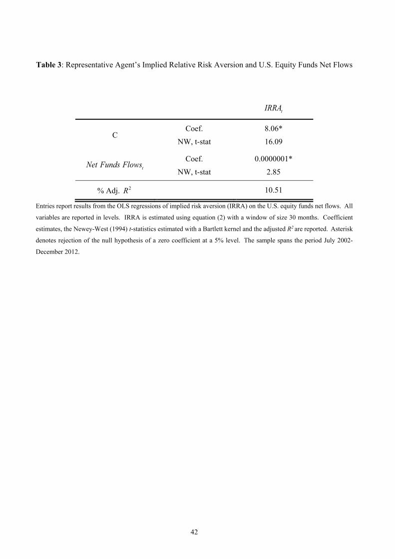
Table 3: Representative Agent’s Implied Relative Risk Aversion and U.S. Equity Funds Net Flows

tIRRA

CCoef.

NW, t-stat

8.06*

16.09

tNet Funds FlowsCoef.

NW, t-stat

0.0000001*

2.85

% Adj. 2R 10.51

Entries report results from the OLS regressions of implied risk aversion (IRRA) on the U.S. equity funds net flows. All

variables are reported in levels. IRRA is estimated using equation (2) with a window of size 30 months. Coefficient

estimates, the Newey-West (1994) t-statistics estimated with a Bartlett kernel and the adjusted R2 are reported. Asterisk

denotes rejection of the null hypothesis of a zero coefficient at a 5% level. The sample spans the period July 2002-

December 2012.

42

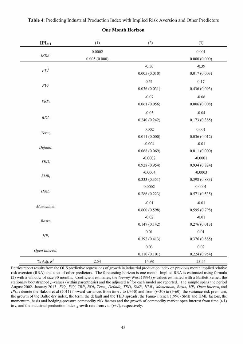
Table 4: Predicting Industrial Production Index with Implied Risk Aversion and Other Predictors

One Month Horizon

IPIt+1 (1) (2) (3)

IRRAt0.0002

0.005 (0.000)

0.001

0.000 (0.000)

FVt1

-0.50

0.005 (0.010)

-0.39

0.017 (0.003)

FVt2

0.51

0.036 (0.031)

0.17

0.436 (0.093)

VRPt

-0.07

0.061 (0.056)

-0.06

0.006 (0.008)

BDIt

-0.03

0.240 (0.242)

-0.04

0.173 (0.385)

Termt0.002

0.011 (0.000)

0.001

0.036 (0.012)

Defaultt-0.004

0.068 (0.069)

-0.01

0.011 (0.000)

TEDt-0.0002

0.928 (0.954)

-0.0001

0.934 (0.824)

SMBt-0.0004

0.333 (0.351)

-0.0003

0.398 (0.883)

HMLt

0.0002

0.286 (0.223)

0.0001

0.571 (0.535)

Momentumt-0.01

0.600 (0.598)

-0.01

0.595 (0.798)

Basist-0.02

0.147 (0.142)

-0.01

0.276 (0.013)

HPt

0.01

0.392 (0.413)

0.01

0.376 (0.885)

Open Interestt0.03

0.110 (0.101)

0.02

0.224 (0.954)

% Adj. R2 2.54 14.98 23.54Entries report results from the OLS predictive regressions of growth in industrial production index on previous month implied relative risk aversion (RRA) and a set of other predictors. The forecasting horizon is one month. Implied RRA is estimated using formula (2) with a window of size 30 months. Coefficient estimates, the Newey-West (1994) p-values estimated with a Bartlett kernel, the stationary bootstrapped p-values (within parenthesis) and the adjusted R2 for each model are reported. The sample spans the periodAugust 2002- January 2013. FVt

1, FVt2, VRPt, BDIt, Termt, Defaultt, TEDt, SMBt, HMLt, Momentumt, Basist, HPt, Open Interestt and

IPIt+1 denote the Bakshi et al (2011) forward variances from time t to (t+30) and from (t+30) to (t+60), the variance risk premium, the growth of the Baltic dry index, the term, the default and the TED spreads, the Fama- French (1996) SMB and HML factors, the momentum, basis and hedging-pressure commodity risk factors and the growth of commodity market open interest from time (t-1) to t, and the industrial production index growth rate from t to (t+1), respectively.

43

Table 5: Predicting Nonfarm Payroll Employment with Implied Risk Aversion and Other Predictors

One Month Horizon

Payrollt+1 (1) (2) (3)

IRRAt0.0001

0.000 (0.000)0.0003

0.000 (0.000)

FVt1

-0.130.074 (0.066)

-0.050.388 (0.000)

FVt2

0.130.147 (0.138)

-0.110.060 (0.000)

VRPt-0.004

0.730 (0.738)0.00001

0.988 (0.869)

BDIt-0.01

0.511 (0.515)-0.01

0.039 (0.016)

Termt0.001

0.103 (0.030)0.0001

0.363 (0.847)

Defaultt-0.001

0.361 (0.325)-0.001

0.002 (0.000)

TEDt-0.0002

0.810 (0.810)-0.0001

0.738 (0.005)

SMBt-0.00001

0.224 (0.251)-0.00004

0.359 (0.436)

HMLt0.00001

0.449 (0.537)-0.000001

0.868 (0.700)

Momentumt-0.004

0.212 (0.208)-0.004

0.030 (0.002)

Basist-0.01

0.061 (0.068)-0.002

0.139 (0.367)

HPt0.003

0.505 (0.534)0.003

0.032 (0.979)

Open Interestt0.01

0.043 (0.050)0.0003

0.893 (0.733)

% Adj. R2 10.47 18.89 76.90

Entries report results from the OLS predictive regressions of growth in nonfarm payroll employment on previous month implied relative risk aversion (RRA) and a set of other predictors. The forecasting horizon is one month. Implied RRA is estimated using formula (2) with a window of size 30 months. Coefficient estimates, the Newey-West (1994) p-values estimated with a Bartlett kernel, the stationary bootstrapped p-values (within parenthesis) and the adjusted R2 for each model are reported. The sample spans the period August 2002- January 2013. FVt

1, FVt

2, VRPt, BDIt, Termt, Defaultt, TEDt, SMBt, HMLt, Momentumt, Basist, HPt, Open Interestt and Payrollt+1 denote the Bakshi et al (2011)

forward variances from time t to (t+30) and from (t+30) to (t+60), variance risk premium, growth of the Baltic dry index, term, the default and the TED spreads, Fama- French (1996) SMB and HML factors, momentum, basis and hedging-pressure commodity risk factors, growth of commodity market open interest from time (t-1) to t, and the nonfarm payroll employment growth rate from t to (t+1), respectively.

44

Table 6: Predicting the Kansas City Financial Stress Index with Implied Risk Aversion and Other Predictors

One Month Horizon

KCFSIt+1 (1) (2) (3)

IRRAt-0.32

0.001 (0.000)

-0.02

0.000 (0.000)

FVt1

87.67

0.034 (0.027)

45.75

0.223 (0.000)

FVt2

-78.38

0.137 (0.139)

49.03

0.044 (0.853)

VRPt

2.26

0.635 (0.658)

0.73

0.810 (0.555)

BDIt-4.78

0.531 (0.539)

-2.86

0.460 (0.000)

Termt-0.16

0.315 (0.168)

0.04

0.396 (0.000)

Defaultt0.38

0.501 (0.494)

0.55

0.009 (0.000)

TEDt0.68

0.131 (0.112)

0.67

0.047 (0.019)

SMBt

0.05

0.120 (0.144)

0.02

0.074 (0.041)

HMLt

-0.07

0.241 (0.410)

-0.03

0.266 (0.000)

Momentumt

0.09

0.952 (0.959)

0.31

0.662 (0.295)

Basist

2.12

0.250 (0.261)

0.10

0.878 (0.886)

HPt0.86

0.663 (0.681)

0.48

0.425 (0.101)

Open Interestt-4.33

0.031 (0.034)

-0.12

0.862 (0.031)

% Adj. R2 40.99 43.53 87.98Entries report results from the OLS predictive regressions of KCFSI index on previous month implied relative risk aversion (RRA)and a set of other predictors. The forecasting horizon is one month. Implied RRA is estimated using formula (2) with a window of size 30 months. Coefficient estimates, the Newey-West (1994) p-values estimated with a Bartlett kernel, the stationary bootstrapped p-values (within parenthesis) and the adjusted R2 for each model are reported. The sample spans the period August 2002- January2013. FVt

1, FVt2

, VRPt, BDIt, Termt, Defaultt, TEDt, SMBt, HMLt, Momentumt, Basist, HPt, Open Interestt and KCFSIt+1 denote the Bakshi et al (2011) forward variances from time t to (t+30) and from (t+30) to (t+60), the variance risk premium, the growth of the Baltic dry index, the term, the default and the TED spreads, the Fama- French (1996) SMB and HML factors, the momentum, basis and hedging-pressure commodity risk factors and the growth of commodity market open interest from time (t-1) to t, and the Kansas city financial stress index from t to (t+1), respectively.

45

Table 7: Predicting Industrial Production Index with Implied Risk Aversion and Other Predictors

Long Horizons

Panel A

IPIt+h3 M 6 M 9 M 12 M

IRRAt

Coefficients

NW t-stats

Hodrick t-stats

Bootstrap p-values

0.001

2.93

(2.81)

[0.000]

0.001

2.75

(3.04)

[0.000]

0.001

2.36

(2.73)

[0.000]

0.002

2.04

(2.45)

[0.000]

% Adj. R2 4.28 4.19 3.38 2.59

46

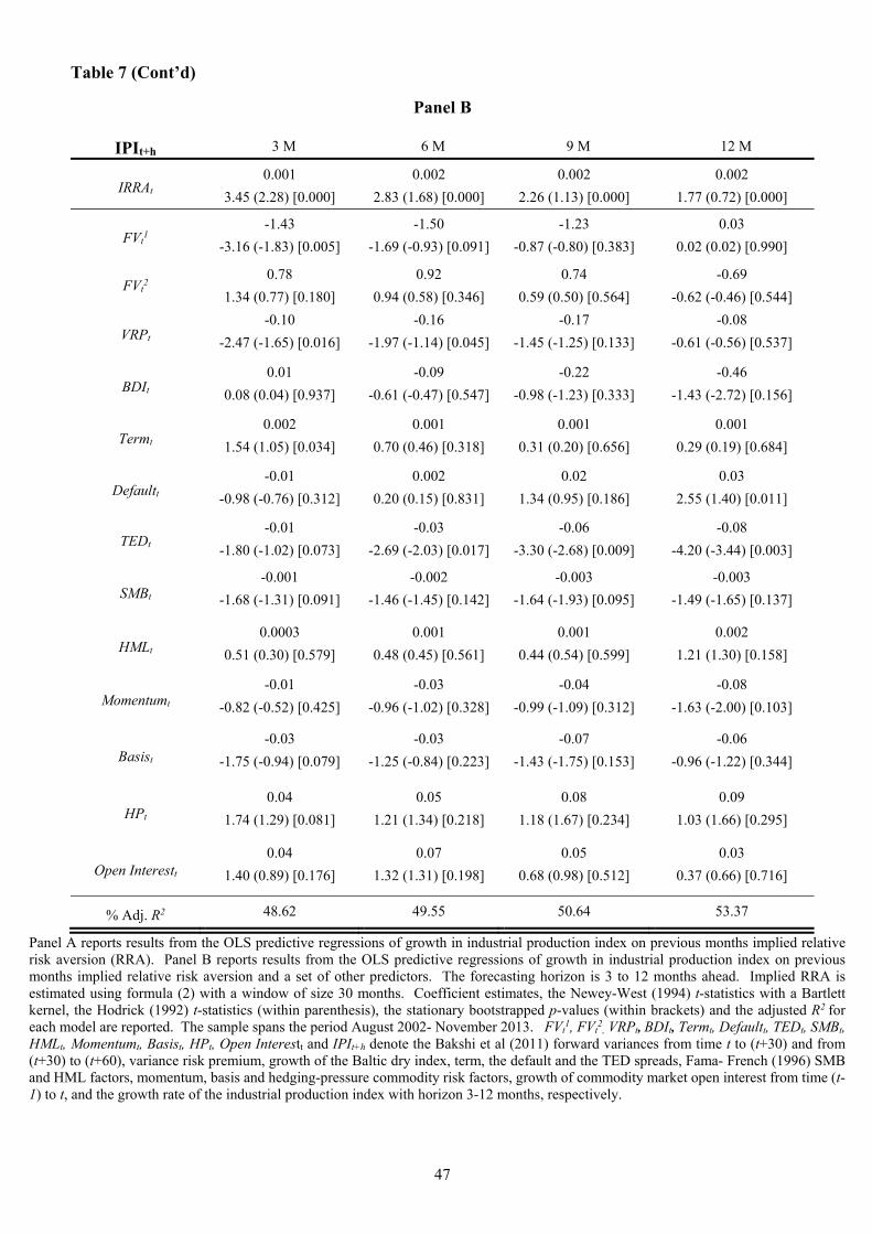
Table 7 (Cont’d)

Panel B

IPIt+h 3 M 6 M 9 M 12 M

IRRAt0.001

3.45 (2.28) [0.000]0.002

2.83 (1.68) [0.000]0.002

2.26 (1.13) [0.000]0.002

1.77 (0.72) [0.000]

FVt1

-1.43-3.16 (-1.83) [0.005]

-1.50-1.69 (-0.93) [0.091]

-1.23-0.87 (-0.80) [0.383]

0.030.02 (0.02) [0.990]

FVt2

0.781.34 (0.77) [0.180]

0.920.94 (0.58) [0.346]

0.740.59 (0.50) [0.564]

-0.69-0.62 (-0.46) [0.544]

VRPt

-0.10-2.47 (-1.65) [0.016]

-0.16-1.97 (-1.14) [0.045]

-0.17-1.45 (-1.25) [0.133]

-0.08-0.61 (-0.56) [0.537]

BDIt

0.010.08 (0.04) [0.937]

-0.09-0.61 (-0.47) [0.547]

-0.22-0.98 (-1.23) [0.333]

-0.46-1.43 (-2.72) [0.156]

Termt

0.0021.54 (1.05) [0.034]

0.0010.70 (0.46) [0.318]

0.0010.31 (0.20) [0.656]

0.0010.29 (0.19) [0.684]

Defaultt

-0.01-0.98 (-0.76) [0.312]

0.0020.20 (0.15) [0.831]

0.021.34 (0.95) [0.186]

0.032.55 (1.40) [0.011]

TEDt-0.01

-1.80 (-1.02) [0.073]-0.03

-2.69 (-2.03) [0.017]-0.06

-3.30 (-2.68) [0.009]-0.08

-4.20 (-3.44) [0.003]

SMBt

-0.001-1.68 (-1.31) [0.091]

-0.002-1.46 (-1.45) [0.142]

-0.003-1.64 (-1.93) [0.095]

-0.003-1.49 (-1.65) [0.137]

HMLt

0.00030.51 (0.30) [0.579]

0.0010.48 (0.45) [0.561]

0.0010.44 (0.54) [0.599]

0.0021.21 (1.30) [0.158]

Momentumt

-0.01-0.82 (-0.52) [0.425]

-0.03-0.96 (-1.02) [0.328]

-0.04-0.99 (-1.09) [0.312]

-0.08-1.63 (-2.00) [0.103]

Basist

-0.03-1.75 (-0.94) [0.079]

-0.03-1.25 (-0.84) [0.223]

-0.07-1.43 (-1.75) [0.153]

-0.06-0.96 (-1.22) [0.344]

HPt

0.041.74 (1.29) [0.081]

0.051.21 (1.34) [0.218]

0.081.18 (1.67) [0.234]

0.091.03 (1.66) [0.295]

Open Interestt

0.041.40 (0.89) [0.176]

0.071.32 (1.31) [0.198]

0.050.68 (0.98) [0.512]

0.030.37 (0.66) [0.716]

% Adj. R2 48.62 49.55 50.64 53.37

Panel A reports results from the OLS predictive regressions of growth in industrial production index on previous months implied relative risk aversion (RRA). Panel B reports results from the OLS predictive regressions of growth in industrial production index on previousmonths implied relative risk aversion and a set of other predictors. The forecasting horizon is 3 to 12 months ahead. Implied RRA is estimated using formula (2) with a window of size 30 months. Coefficient estimates, the Newey-West (1994) t-statistics with a Bartlett kernel, the Hodrick (1992) t-statistics (within parenthesis), the stationary bootstrapped p-values (within brackets) and the adjusted R2 for each model are reported. The sample spans the period August 2002- November 2013. FVt

1, FVt2

, VRPt, BDIt, Termt, Defaultt, TEDt, SMBt, HMLt, Momentumt, Basist, HPt, Open Interestt and IPIt+h denote the Bakshi et al (2011) forward variances from time t to (t+30) and from (t+30) to (t+60), variance risk premium, growth of the Baltic dry index, term, the default and the TED spreads, Fama- French (1996) SMB and HML factors, momentum, basis and hedging-pressure commodity risk factors, growth of commodity market open interest from time (t-1) to t, and the growth rate of the industrial production index with horizon 3-12 months, respectively.

47

Table 8: Predicting Nonfarm Payroll Employment with Implied Risk Aversion and Other Predictors

Long Horizons

Panel A

Payrollt+h3 M 6 M 9 M 12 M

IRRAt

Coefficients

NW t-stats

Hodrick t-stats

Bootstrap p-values

0.002

3.34

(1.67)

[0.045]

0.003

3.11

(1.68)

[0.058]

0.004

2.94

(1.66)

[0.063]

0.005

2.77

(1.59)

[0.086]

% Adj. R2 43.60 40.21 36.03 30.34

48

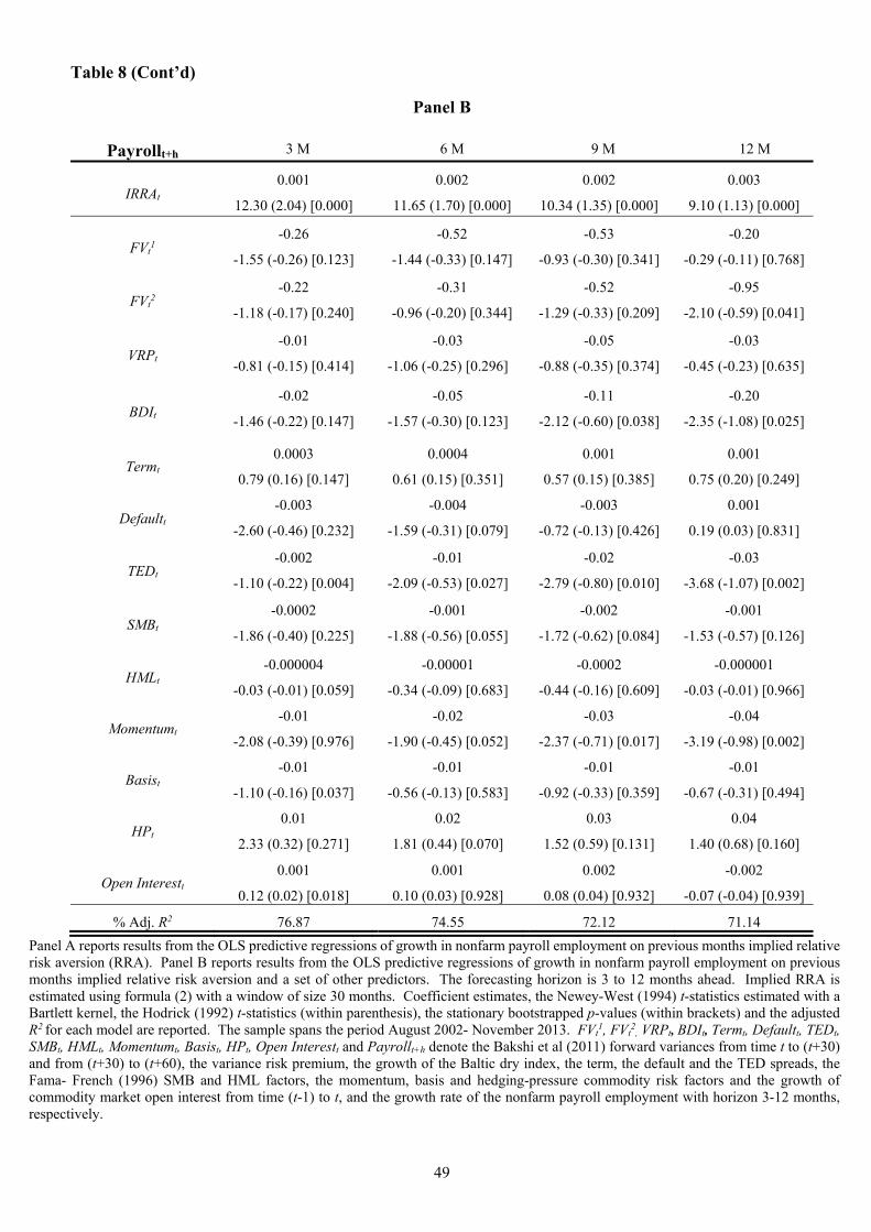
Table 8 (Cont’d)

Panel B

Payrollt+h 3 M 6 M 9 M 12 M

IRRAt0.001

12.30 (2.04) [0.000]

0.002

11.65 (1.70) [0.000]

0.002

10.34 (1.35) [0.000]

0.003

9.10 (1.13) [0.000]

FVt1

-0.26

-1.55 (-0.26) [0.123]

-0.52

-1.44 (-0.33) [0.147]

-0.53

-0.93 (-0.30) [0.341]

-0.20

-0.29 (-0.11) [0.768]

FVt2

-0.22

-1.18 (-0.17) [0.240]

-0.31

-0.96 (-0.20) [0.344]

-0.52

-1.29 (-0.33) [0.209]

-0.95

-2.10 (-0.59) [0.041]

VRPt

-0.01

-0.81 (-0.15) [0.414]

-0.03

-1.06 (-0.25) [0.296]

-0.05

-0.88 (-0.35) [0.374]

-0.03

-0.45 (-0.23) [0.635]

BDIt

-0.02

-1.46 (-0.22) [0.147]

-0.05

-1.57 (-0.30) [0.123]

-0.11

-2.12 (-0.60) [0.038]

-0.20

-2.35 (-1.08) [0.025]

Termt0.0003

0.79 (0.16) [0.147]

0.0004

0.61 (0.15) [0.351]

0.001

0.57 (0.15) [0.385]

0.001

0.75 (0.20) [0.249]

Defaultt-0.003

-2.60 (-0.46) [0.232]

-0.004

-1.59 (-0.31) [0.079]

-0.003

-0.72 (-0.13) [0.426]

0.001

0.19 (0.03) [0.831]

TEDt-0.002

-1.10 (-0.22) [0.004]

-0.01

-2.09 (-0.53) [0.027]

-0.02

-2.79 (-0.80) [0.010]

-0.03

-3.68 (-1.07) [0.002]

SMBt

-0.0002

-1.86 (-0.40) [0.225]

-0.001

-1.88 (-0.56) [0.055]

-0.002

-1.72 (-0.62) [0.084]

-0.001

-1.53 (-0.57) [0.126]

HMLt-0.000004

-0.03 (-0.01) [0.059]

-0.00001

-0.34 (-0.09) [0.683]

-0.0002

-0.44 (-0.16) [0.609]

-0.000001

-0.03 (-0.01) [0.966]

Momentumt-0.01

-2.08 (-0.39) [0.976]

-0.02

-1.90 (-0.45) [0.052]

-0.03

-2.37 (-0.71) [0.017]

-0.04

-3.19 (-0.98) [0.002]

Basist-0.01

-1.10 (-0.16) [0.037]

-0.01

-0.56 (-0.13) [0.583]

-0.01

-0.92 (-0.33) [0.359]

-0.01

-0.67 (-0.31) [0.494]

HPt0.01

2.33 (0.32) [0.271]

0.02

1.81 (0.44) [0.070]

0.03

1.52 (0.59) [0.131]

0.04

1.40 (0.68) [0.160]

Open Interestt0.001

0.12 (0.02) [0.018]

0.001

0.10 (0.03) [0.928]

0.002

0.08 (0.04) [0.932]

-0.002

-0.07 (-0.04) [0.939]

% Adj. R2 76.87 74.55 72.12 71.14Panel A reports results from the OLS predictive regressions of growth in nonfarm payroll employment on previous months implied relative risk aversion (RRA). Panel B reports results from the OLS predictive regressions of growth in nonfarm payroll employment on previous months implied relative risk aversion and a set of other predictors. The forecasting horizon is 3 to 12 months ahead. Implied RRA is estimated using formula (2) with a window of size 30 months. Coefficient estimates, the Newey-West (1994) t-statistics estimated with aBartlett kernel, the Hodrick (1992) t-statistics (within parenthesis), the stationary bootstrapped p-values (within brackets) and the adjustedR2 for each model are reported. The sample spans the period August 2002- November 2013. FVt

1, FVt2

, VRPt, BDIt, Termt, Defaultt, TEDt, SMBt, HMLt, Momentumt, Basist, HPt, Open Interestt and Payrollt+h denote the Bakshi et al (2011) forward variances from time t to (t+30) and from (t+30) to (t+60), the variance risk premium, the growth of the Baltic dry index, the term, the default and the TED spreads, the Fama- French (1996) SMB and HML factors, the momentum, basis and hedging-pressure commodity risk factors and the growth of commodity market open interest from time (t-1) to t, and the growth rate of the nonfarm payroll employment with horizon 3-12 months, respectively.

49

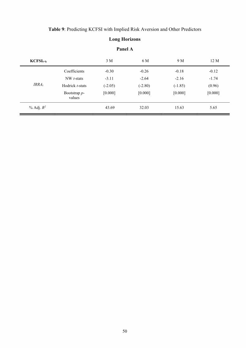
Table 9: Predicting KCFSI with Implied Risk Aversion and Other Predictors

Long Horizons

Panel A

KCFSIt+h 3 M 6 M 9 M 12 M

IRRAt

Coefficients

NW t-stats

Hodrick t-stats

Bootstrap p-values

-0.30

-3.11

(-2.05)

[0.000]

-0.26

-2.64

(-2.80)

[0.000]

-0.18

-2.16

(-1.85)

[0.000]

-0.12

-1.74

(0.96)

[0.000]

% Adj. R2 43.69 32.03 15.63 5.65

50

Table 9 (Cont’d)

Panel B

KCFSIt+h 3 M 6 M 9 M 12 M

IRRAt

-0.14

-9.37 (-2.79) [0.000]

-0.10

-4.72 (-1.07)[0.000]

-0.06

-2.31 (-0.43) [0.000]

-0.03

-0.97 (-0.13) [0.072]

FVt1

30.65

0.78 (0.27) [0.397]

-16.96

-0.40 (-0.10)[0.671]

-72.36

-1.70 (-0.45) [0.097]

-128.76

-4.47 (-0.71) [0.000]

FVt2

23.53

1.06 (0.16) [0.275]

17.60

0.66 (0.10) [0.509]

48.97

1.72 (0.30) [0.094]

95.45

2.61 (0.55) [0.012]

VRPt

3.04

0.81 (0.46) [0.400]

-0.20

-0.06 (-0.02)[0.947]

-4.28

-1.08 (-0.33) [0.284]

-8.22

-2.43 (-0.54) [0.016]

BDIt

-0.93

-0.33 (-0.06) [0.744]

5.59

0.92 (0.33) [0.369]

13.23

1.27 (0.76) [0.206]

10.20

1.13 (0.62) [0.248]

Termt0.10

1.87 (0.64) [0.010]

0.14

1.51 (0.51) [0.036]

0.04

0.36 (0.10) [0.609]

-0.05

-0.43 (-0.09) [0.517]

Defaultt

0.26

1.05 (0.38) [0.241]

-0.20

-0.63 (-0.19)[0.509]

-0.28

-0.76 (-0.19) [0.434]

-0.54

-1.54 (-0.29) [0.105]

TEDt1.18

3.46 (0.94) [0.005]

1.80

3.43 (0.86) [0.006]

1.87

3.27 (0.65) [0.013]

2.21

4.05 (0.67) [0.000]

SMBt0.04

0.96 (0.55) [0.365]

0.06

1.32 (0.50) [0.185]

0.01

0.30 (0.10) [0.759]

-0.03

-1.20 (-0.28) [0.225]

HMLt

-0.02

-0.46 (-0.17) [0.586]

-0.02

-0.82 (-0.19)[0.312]

-0.0003

-0.01 (-0.003) [0.994]

-0.07

-1.71 (-0.52) [0.055]

Momentumt

0.47

0.44 (0.17) [0.641]

0.62

0.59 (0.22) [0.538]

2.13

1.45 (0.65) [0.136]

1.75

1.21 (0.43) [0.206]

Basist

-1.03

-1.16 (-0.58) [0.259]

0.83

0.43 (0.22) [0.679]

-0.49

-0.26 (-0.13) [0.786]

-1.18

-0.71 (-0.28) [0.479]

HPt

-0.19

-0.22 (-0.08) [0.840]

-2.41

-0.91 (-0.53)[0.363]

0.27

0.09 (0.05) [0.928]

3.09

1.02 (0.60) [0.318]

Open Interestt

-0.49

-0.26 (-0.13) [0.800]

-1.50

-0.77 (-0.29)[0.448]

-0.07

-0.03 (-0.01) [0.984]

3.55

1.18 (0.64) [0.231]

% Adj. R2 71.78 55.32 36.99 47.02

Panel A reports results from the OLS predictive regressions of KCFSI index on previous months implied relative risk aversion (RRA). Panel B reports results from the OLS predictive regressions of KCFSI index on previous months implied relative risk aversion (RRA) and a set of other predictors. The forecasting horizon is 3 to 12 months ahead. Implied RRA is estimated using formula (2) with a window of size 30 months. Coefficient estimates, the Newey-West (1994) t-statistics with a Bartlett kernel, the Hodrick (1992) t-statistics (within parenthesis), the stationary bootstrapped p-values (within brackets) and the adjusted R2 for each model are reported. The sample spans the period August

51

2002- November 2013. FVt1, FVt

2, VRPt, BDIt, Termt, Defaultt, TEDt, SMBt, HMLt, Momentumt, Basist, HPt, Open Interestt and KCFSIt+h

denote the Bakshi et al (2011) forward variances from time t to (t+30) and from (t+30) to (t+60), the variance risk premium, the growth of the Baltic dry index, the term, the default and the TED spreads, the Fama- French (1996) SMB and HML factors, the momentum, basis and hedging-pressure commodity risk factors and the growth of commodity market open interest from time (t-1) to t, and the Kansas city financial stress index with horizon 3-12 months, respectively.

52

Table 10: Predicting Real Economic Activity with Orthogonalized Implied Risk Aversion

One Month Horizon

IPIt+1

(1)

Payrollt+1

(2)

KCFSIt+1

(3)

IRRA_Orthog.t0.001

0.000 (0.000)

0.0003

0.000 (0.000)

-0.15

0.000 (0.000)

FVt1

-0.11

0.584 (0.006)

0.14

0.029 (0.000)

-59.48

0.140 (0.000)

FVt2

0.06

0.806 (0.082)

-0.18

0.002 (0.000)

93.59

0.000 (0.851)

VRPt-0.05

0.034 (0.012)

0.01

0.062 (0.856)

-4.88

0.149 (0.584)

BDIt-0.04

0.159 (0.384)

-0.01

0.025 (0.014)

-2.09

0.561 (0.000)

Termt0.001

0.018 (0.026)

0.0002

0.106 (0.949)

0.01

0.845 (0.000)

Defaultt-0.04

0.015 (0.002)

-0.001

0.009 (0.000)

0.42

0.030 (0.000)

TEDt-0.0004

0.780 (0.817)

-0.0003

0.430 (0.016)

0.77

0.020 (0.003)

SMBt-0.0003

0.390 (0.890)

-0.0001

0.319 (0.424)

0.03

0.038 (0.034)

HMLt0.0001

0.589 (0.452)

-0.00001

0.765 (0.683)

-0.02

0.323 (0.000)

Momentumt-0.005

0.598 (0.788)

-0.004

0.023 (0.004)

0.30

0.649 (0.288)

Basist-0.01

0.258 (0.016)

-0.003

0.122 (0.364)

0.18

0.769 (0.891)

HPt0.013

0.370 (0.889)

0.003

0.029 (0.984)

0.40

0.481 (0.075)

Open Interestt0.02

0.240 (0.954)

0.0001

0.977 (0.722)

0.09

0.899 (0.027)

% Adj. R2 23.29 75.44 88.97Entries report results from the OLS predictive regressions of growth in industrial production index, growth in nonfarm payroll employment and KCFSI index on previous month orthogonalized implied relative risk aversion (RRA_Orthog.) and a set of other predictors. The forecasting horizon is one month. Implied RRA is estimated using formula (2) with a window of size 30 months. Coefficient estimates, the Newey-West (1994) p-values estimated with a Bartlett kernel, the stationary bootstrapped p-values (within parenthesis) and the adjusted R2 for each model are reported. The sample spans the period August 2002- January 2013. FVt

1, FVt2

,VRPt, BDIt, Termt, Defaultt, TEDt, SMBt, HMLt, Momentumt, Basist, HPt, Open Interestt, IPIt+1, Payrollt+1 and KCFSIt+1 denote the Bakshi et al (2011) forward variances from time t to (t+30) and from (t+30) to (t+60), the variance risk premium, the growth of the Baltic dry index, the term, the default and the TED spreads, the Fama- French (1996) SMB and HML factors, the momentum, basis and hedging-pressure commodity risk factors and the growth of commodity market open interest from time (t-1) to t, the industrial production index growth rate from t to (t+1), the nonfarm payroll employment growth rate from t to (t+1), and the Kansas city financial stress index from t to (t+1), respectively.

53

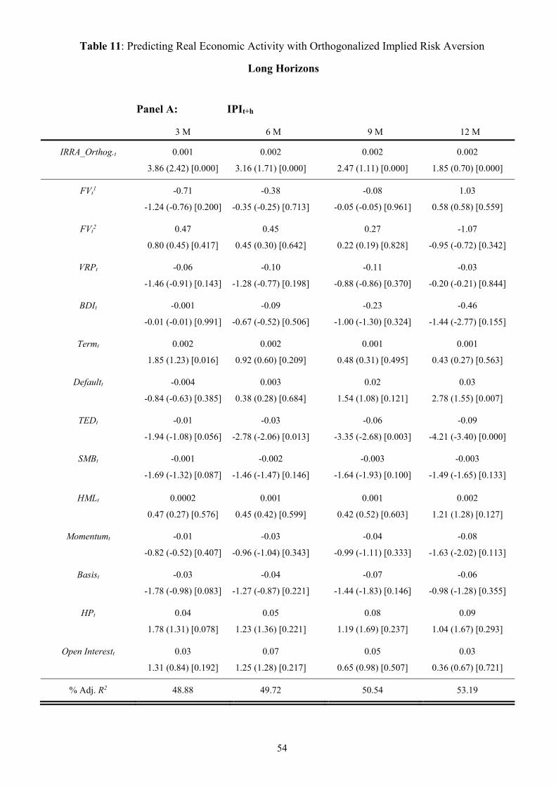
Table 11: Predicting Real Economic Activity with Orthogonalized Implied Risk Aversion

Long Horizons

Panel A: IPIt+h

3 M 6 M 9 M 12 M

IRRA_Orthog.t 0.001

3.86 (2.42) [0.000]

0.002

3.16 (1.71) [0.000]

0.002

2.47 (1.11) [0.000]

0.002

1.85 (0.70) [0.000]

FVt1 -0.71

-1.24 (-0.76) [0.200]

-0.38

-0.35 (-0.25) [0.713]

-0.08

-0.05 (-0.05) [0.961]

1.03

0.58 (0.58) [0.559]

FVt2 0.47

0.80 (0.45) [0.417]

0.45

0.45 (0.30) [0.642]

0.27

0.22 (0.19) [0.828]

-1.07

-0.95 (-0.72) [0.342]

VRPt -0.06

-1.46 (-0.91) [0.143]

-0.10

-1.28 (-0.77) [0.198]

-0.11

-0.88 (-0.86) [0.370]

-0.03

-0.20 (-0.21) [0.844]

BDIt -0.001

-0.01 (-0.01) [0.991]

-0.09

-0.67 (-0.52) [0.506]

-0.23

-1.00 (-1.30) [0.324]

-0.46

-1.44 (-2.77) [0.155]

Termt 0.002

1.85 (1.23) [0.016]

0.002

0.92 (0.60) [0.209]

0.001

0.48 (0.31) [0.495]

0.001

0.43 (0.27) [0.563]

Defaultt -0.004

-0.84 (-0.63) [0.385]

0.003

0.38 (0.28) [0.684]

0.02

1.54 (1.08) [0.121]

0.03

2.78 (1.55) [0.007]

TEDt -0.01

-1.94 (-1.08) [0.056]

-0.03

-2.78 (-2.06) [0.013]

-0.06

-3.35 (-2.68) [0.003]

-0.09

-4.21 (-3.40) [0.000]

SMBt -0.001

-1.69 (-1.32) [0.087]

-0.002

-1.46 (-1.47) [0.146]

-0.003

-1.64 (-1.93) [0.100]

-0.003

-1.49 (-1.65) [0.133]

HMLt 0.0002

0.47 (0.27) [0.576]

0.001

0.45 (0.42) [0.599]

0.001

0.42 (0.52) [0.603]

0.002

1.21 (1.28) [0.127]

Momentumt -0.01

-0.82 (-0.52) [0.407]

-0.03

-0.96 (-1.04) [0.343]

-0.04

-0.99 (-1.11) [0.333]

-0.08

-1.63 (-2.02) [0.113]

Basist -0.03

-1.78 (-0.98) [0.083]

-0.04

-1.27 (-0.87) [0.221]

-0.07

-1.44 (-1.83) [0.146]

-0.06

-0.98 (-1.28) [0.355]

HPt 0.04

1.78 (1.31) [0.078]

0.05

1.23 (1.36) [0.221]

0.08

1.19 (1.69) [0.237]

0.09

1.04 (1.67) [0.293]

Open Interestt 0.03

1.31 (0.84) [0.192]

0.07

1.25 (1.28) [0.217]

0.05

0.65 (0.98) [0.507]

0.03

0.36 (0.67) [0.721]

% Adj. R2 48.88 49.72 50.54 53.19

54

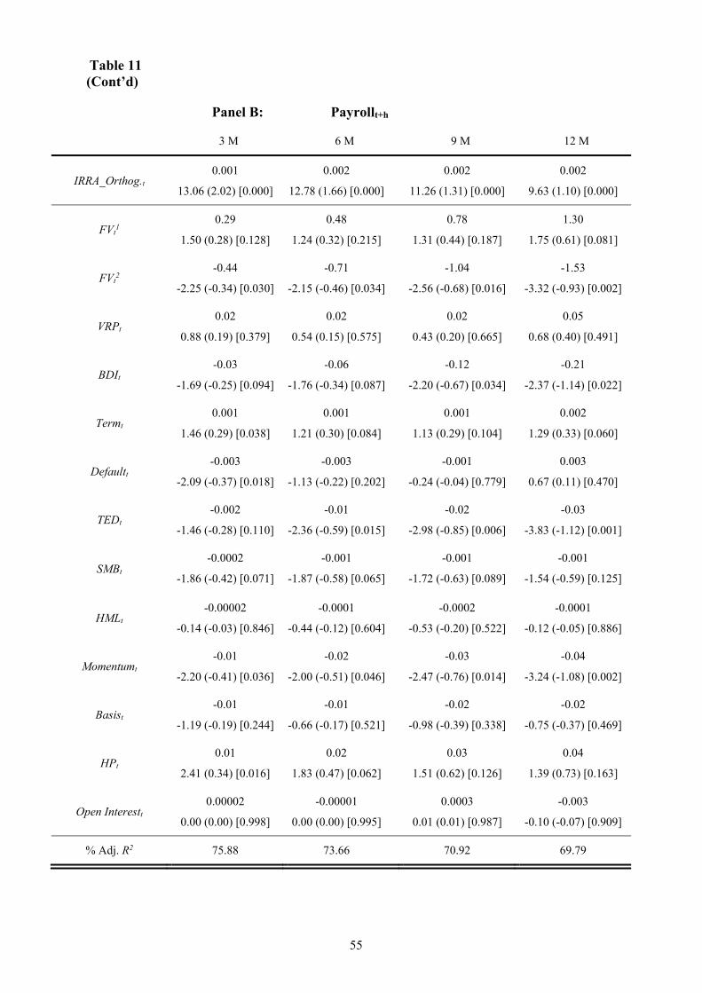
Table 11(Cont’d)

Panel B: Payrollt+h

3 M 6 M 9 M 12 M

IRRA_Orthog.t0.001

13.06 (2.02) [0.000]

0.002

12.78 (1.66) [0.000]

0.002

11.26 (1.31) [0.000]

0.002

9.63 (1.10) [0.000]

FVt1

0.29

1.50 (0.28) [0.128]

0.48

1.24 (0.32) [0.215]

0.78

1.31 (0.44) [0.187]

1.30

1.75 (0.61) [0.081]

FVt2

-0.44

-2.25 (-0.34) [0.030]

-0.71

-2.15 (-0.46) [0.034]

-1.04

-2.56 (-0.68) [0.016]

-1.53

-3.32 (-0.93) [0.002]

VRPt0.02

0.88 (0.19) [0.379]

0.02

0.54 (0.15) [0.575]

0.02

0.43 (0.20) [0.665]

0.05

0.68 (0.40) [0.491]

BDIt-0.03

-1.69 (-0.25) [0.094]

-0.06

-1.76 (-0.34) [0.087]

-0.12

-2.20 (-0.67) [0.034]

-0.21

-2.37 (-1.14) [0.022]

Termt0.001

1.46 (0.29) [0.038]

0.001

1.21 (0.30) [0.084]

0.001

1.13 (0.29) [0.104]

0.002

1.29 (0.33) [0.060]

Defaultt-0.003

-2.09 (-0.37) [0.018]

-0.003

-1.13 (-0.22) [0.202]

-0.001

-0.24 (-0.04) [0.779]

0.003

0.67 (0.11) [0.470]

TEDt-0.002

-1.46 (-0.28) [0.110]

-0.01

-2.36 (-0.59) [0.015]

-0.02

-2.98 (-0.85) [0.006]

-0.03

-3.83 (-1.12) [0.001]

SMBt-0.0002

-1.86 (-0.42) [0.071]

-0.001

-1.87 (-0.58) [0.065]

-0.001

-1.72 (-0.63) [0.089]

-0.001

-1.54 (-0.59) [0.125]

HMLt-0.00002

-0.14 (-0.03) [0.846]

-0.0001

-0.44 (-0.12) [0.604]

-0.0002

-0.53 (-0.20) [0.522]

-0.0001

-0.12 (-0.05) [0.886]

Momentumt-0.01

-2.20 (-0.41) [0.036]

-0.02

-2.00 (-0.51) [0.046]

-0.03

-2.47 (-0.76) [0.014]

-0.04

-3.24 (-1.08) [0.002]

Basist-0.01

-1.19 (-0.19) [0.244]

-0.01

-0.66 (-0.17) [0.521]

-0.02

-0.98 (-0.39) [0.338]

-0.02

-0.75 (-0.37) [0.469]

HPt0.01

2.41 (0.34) [0.016]

0.02

1.83 (0.47) [0.062]

0.03

1.51 (0.62) [0.126]

0.04

1.39 (0.73) [0.163]

Open Interestt0.00002

0.00 (0.00) [0.998]

-0.00001

0.00 (0.00) [0.995]

0.0003

0.01 (0.01) [0.987]

-0.003

-0.10 (-0.07) [0.909]

% Adj. R2 75.88 73.66 70.92 69.79

55

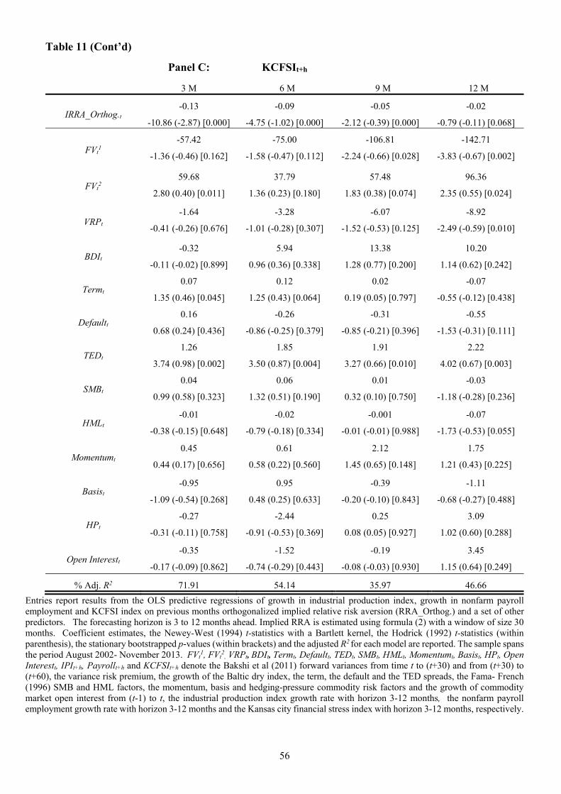
Table 11 (Cont’d)

Panel C: KCFSIt+h

3 M 6 M 9 M 12 M

IRRA_Orthog.t-0.13

-10.86 (-2.87) [0.000]

-0.09

-4.75 (-1.02) [0.000]

-0.05

-2.12 (-0.39) [0.000]

-0.02

-0.79 (-0.11) [0.068]

FVt1

-57.42

-1.36 (-0.46) [0.162]

-75.00

-1.58 (-0.47) [0.112]

-106.81

-2.24 (-0.66) [0.028]

-142.71

-3.83 (-0.67) [0.002]

FVt2

59.68

2.80 (0.40) [0.011]

37.79

1.36 (0.23) [0.180]

57.48

1.83 (0.38) [0.074]

96.36

2.35 (0.55) [0.024]

VRPt

-1.64

-0.41 (-0.26) [0.676]

-3.28

-1.01 (-0.28) [0.307]

-6.07

-1.52 (-0.53) [0.125]

-8.92

-2.49 (-0.59) [0.010]

BDIt-0.32

-0.11 (-0.02) [0.899]

5.94

0.96 (0.36) [0.338]

13.38

1.28 (0.77) [0.200]

10.20

1.14 (0.62) [0.242]

Termt0.07

1.35 (0.46) [0.045]

0.12

1.25 (0.43) [0.064]

0.02

0.19 (0.05) [0.797]

-0.07

-0.55 (-0.12) [0.438]

Defaultt0.16

0.68 (0.24) [0.436]

-0.26

-0.86 (-0.25) [0.379]

-0.31

-0.85 (-0.21) [0.396]

-0.55

-1.53 (-0.31) [0.111]

TEDt1.26

3.74 (0.98) [0.002]

1.85

3.50 (0.87) [0.004]

1.91

3.27 (0.66) [0.010]

2.22

4.02 (0.67) [0.003]

SMBt0.04

0.99 (0.58) [0.323]

0.06

1.32 (0.51) [0.190]

0.01

0.32 (0.10) [0.750]

-0.03

-1.18 (-0.28) [0.236]

HMLt-0.01

-0.38 (-0.15) [0.648]

-0.02

-0.79 (-0.18) [0.334]

-0.001

-0.01 (-0.01) [0.988]

-0.07

-1.73 (-0.53) [0.055]

Momentumt

0.45

0.44 (0.17) [0.656]

0.61

0.58 (0.22) [0.560]

2.12

1.45 (0.65) [0.148]

1.75

1.21 (0.43) [0.225]

Basist-0.95

-1.09 (-0.54) [0.268]

0.95

0.48 (0.25) [0.633]

-0.39

-0.20 (-0.10) [0.843]

-1.11

-0.68 (-0.27) [0.488]

HPt-0.27

-0.31 (-0.11) [0.758]

-2.44

-0.91 (-0.53) [0.369]

0.25

0.08 (0.05) [0.927]

3.09

1.02 (0.60) [0.288]

Open Interestt-0.35

-0.17 (-0.09) [0.862]

-1.52

-0.74 (-0.29) [0.443]

-0.19

-0.08 (-0.03) [0.930]

3.45

1.15 (0.64) [0.249]

% Adj. R2 71.91 54.14 35.97 46.66Entries report results from the OLS predictive regressions of growth in industrial production index, growth in nonfarm payroll employment and KCFSI index on previous months orthogonalized implied relative risk aversion (RRA_Orthog.) and a set of other predictors. The forecasting horizon is 3 to 12 months ahead. Implied RRA is estimated using formula (2) with a window of size 30 months. Coefficient estimates, the Newey-West (1994) t-statistics with a Bartlett kernel, the Hodrick (1992) t-statistics (within parenthesis), the stationary bootstrapped p-values (within brackets) and the adjusted R2 for each model are reported. The sample spans the period August 2002- November 2013. FVt

1, FVt2, VRPt, BDIt, Termt, Defaultt, TEDt, SMBt, HMLt, Momentumt, Basist, HPt, Open

Interestt, IPIt+h, Payrollt+h and KCFSIt+h denote the Bakshi et al (2011) forward variances from time t to (t+30) and from (t+30) to (t+60), the variance risk premium, the growth of the Baltic dry index, the term, the default and the TED spreads, the Fama- French (1996) SMB and HML factors, the momentum, basis and hedging-pressure commodity risk factors and the growth of commodity market open interest from (t-1) to t, the industrial production index growth rate with horizon 3-12 months, the nonfarm payroll employment growth rate with horizon 3-12 months and the Kansas city financial stress index with horizon 3-12 months, respectively.

56

FiguresFigure 1: Time variation of Risk -Neutral Moments

The figure shows the time evolution of the daily S&P 500 risk-neutral volatility, skewness and kurtosis

with horizon 30 days over the period January 4th 1996 - December 31st 2012.

00.05

0.10.15

0.20.25

Risk-Neutral Volatility

-4

-3

-2

-1

0

Risk-Neutral Skewness

0

5

10

15

20

Risk-Neutral Kurtosis

57

Figure 2: Implied Risk Aversion and S&P 500

The figure depicts the monthly implied relative risk aversion (IRRA) with a 30 days constant horizon and

the S&P 500 over the period July 2002 - December 2012. IRRA is estimated by the Kang, Kim and Yoon

(2010) formula using an estimation window of size 30 months. Physical variance is estimated with high-

frequency data.

0

500

1000

1500

2000

02468

101214

Implied Risk Aversion vs. S&P 500

RRA, Instruments Set 1

RRA, Instruments Set 2

RRA, Instruments Set 3

S&P 500

58

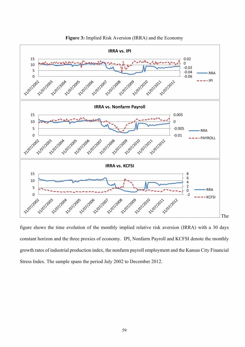
Figure 3: Implied Risk Aversion (IRRA) and the Economy

The

figure shows the time evolution of the monthly implied relative risk aversion (IRRA) with a 30 days

constant horizon and the three proxies of economy. IPI, Nonfarm Payroll and KCFSI denote the monthly

growth rates of industrial production index, the nonfarm payroll employment and the Kansas City Financial

Stress Index. The sample spans the period July 2002 to December 2012.

-0.06-0.04-0.0200.02

05

1015

IRRA vs. IPI

RRA

IPI

-0.01

-0.005

0

0.005

0

5

10

15

IRRA vs. Nonfarm Payroll

RRA

PAYROLL

-202468

0

5

10

15

IRRA vs. KCFSI

RRA

KCFSI

59

Figure 4: Implied Relative Risk Aversion (IRRA) and U.S. equity funds net flows

The figure shows the IRRA and the U.S. equities funds net flows time variation. IRRAis estimated

using formula (2). Equity net flows are reported in millions U.S. dollars. The graph refers to the period

July 2002 - December 2012.

-80-60-40-200204060

02468

101214

Mill

ions

IRRA and Equity Net Cash Flows

RRA

Equity Net Cash Flow

60

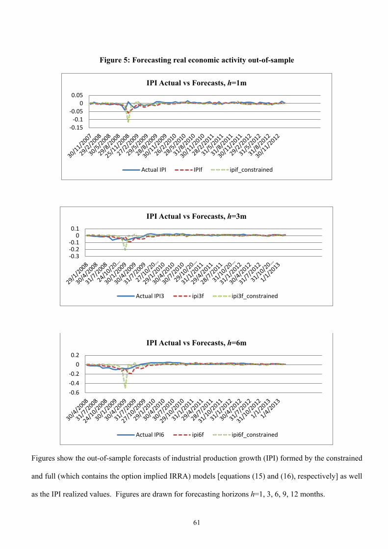
Figure 5: Forecasting real economic activity out-of-sample

Figures show the out-of-sample forecasts of industrial production growth (IPI) formed by the constrained

and full (which contains the option implied IRRA) models [equations (15) and (16), respectively] as well

as the IPI realized values. Figures are drawn for forecasting horizons h=1, 3, 6, 9, 12 months.

-0.15-0.1

-0.050

0.05

IPI Actual vs Forecasts, h=1m

Actual IPI IPIf ipif_constrained

-0.3-0.2-0.1

00.1

IPI Actual vs Forecasts, h=3m

Actual IPI3 ipi3f ipi3f_constrained

-0.6-0.4-0.2

00.2

IPI Actual vs Forecasts, h=6m

Actual IPI6 ipi6f ipi6f_constrained

61

Figure 5 (cont’d): Forecasting real economic activity out-of-sample

Figures show the out-of-sample forecasts of industrial production growth (IPI) formed by the constrained

and full (which contains the option implied IRRA) models [equations (15) and (16), respectively] as well

as the IPI realized values. Figures are drawn for forecasting horizons h=1, 3, 6, 9, 12 months.

-1-0.8-0.6-0.4-0.2

00.2

IPI Actual vs Forecasts, h=9m

Actual IPI9 ipi9f ipi9f_constrained

-1.2-1

-0.8-0.6-0.4-0.2

00.2

IPI Actual vs Forecasts, h=12m

Actual IPI12 ipi12f ipi12f_constrained

62

This working paper has been produced bythe School of Economics and Finance atQueen Mary University of London

Copyright © 2015 Sylvia Sarantopoulou-Chiourea

School of Economics and FinanceQueen Mary University of LondonMile End RoadLondon E1 4NSTel: +44 (0)20 7882 7356Fax: +44 (0)20 8983 3580Web: www.econ.qmul.ac.uk/research/workingpapers/

and George Skiadopoulos. All rights reserved