SCHOOL OF ECONOMICS

Discussion Paper 2003-04

Does Child Labour Affect School Attendance and School Performance?

Multi Country Evidence on SIMPOC Data

Ranjan Ray

and

Geoffrey Lancaster

ISSN 1443-8593 ISBN 1 86295 118 7

FINAL REPORT

Does Child Labour Affect School Attendance and School Performance? Multi Country Evidence on SIMPOC Data

By

Ranjan Ray* and Geoffrey Lancaster

School of Economics University of Tasmania

Hobart Australia

First Draft: May 2003

Revised Version: July 2003

*Correspondence to Ranjan Ray, School of Economics, University of Tasmania, Private Bag 85, Hobart, Tasmania, 7001, Australia. Email: Ranjan.Ray@utas.edu.au. Financial support from the International Labour Organisation is gratefully acknowledged. Views expressed are those of the authors and should not be attributed to the International Labour Organisation. The authors thank Yacouba Diallo, Peter Matz, Hakki Ozel, and Bijoy Raychaudhuri for helpful comments. The disclaimer applies.

Abstract

ILO Convention No. 138, Art. 7(b) stipulates that light work may be permitted as of the age of 12 or 13 provided it does not “prejudice attendance at school” nor “the capacity to benefit from the instruction received”. This raises the issue of the impact of child labour on schooling for children in these age groups. Notwithstanding a large and rapidly expanding literature on child labour, there is not much empirical evidence on this issue since much of this literature has concentrated on analysing the causes of child labour rather than studying its consequences, especially for the child’s learning. The cost of child labour for human capital accumulation has simply been assumed rather than formally investigated. The limited evidence that does exist on this issue makes little or no attempt to control for the endogeneity of child labour hours in the estimation. Such endogeneity can arise because of the reverse causation of child labour by learning disadvantage and lack of necessary intrinsic skills.

The present study seeks to fill this significant gap in the literature on child labour. The exercise is conducted on the data sets involving 12-14 year old children from 7 countries collected under the ILO’s “Statistical Information and Monitoring Programme on Child Labour” (SIMPOC). The chosen countries span a wide spectrum geographically, culturally and in the range of economic development, namely, from the developed European country context of Portugal to poor Afro-Asian countries such as Namibia and Philippines. The list also includes Sri Lanka which, notwithstanding its status as a developing country, has school enrolment rates that approach those in developed countries.

In its investigation of the impact of child labour on the child’s learning, the study attempts to control for the likely endogeneity of child labour hours in the estimation as mentioned above. This paper investigates the sensitivity of the principal qualitative conclusions to the estimation procedure used. The study also provides evidence of the impact of domestic hours on the child’s learning. Wherever possible, the data set is disaggregated between the rural and urban sectors, between boys and girls and, in case of Philippines and Sri Lanka, between the different occupational categories of the employed children. The study widens the scope of the investigation by providing evidence on the impact of child labour hours on time spent on studies at home and on the number of failures experienced by the child at school. In keeping with the spirit of this enquiry, the study allows for turning points in the relationships between schooling and child labour hours by including the child labour hours variable, in both linear and square form, on the right hand side of the estimated equations.

The study provides extensive evidence of the damage done by child labour to the child’s education right from her point of entry to the child labour market. In nearly all the cases, we find robust evidence of strong negative impact of child labour hours on the educational variables, with the marginal impact weakening at the higher levels of work hours. The control for endogeneity seems to worsen the impact of child labour hours on the child’s learning. Other results include the evidence that, generally, boys do worse than girls and children from female headed households fare worse than other children on the various schooling outcomes.

A lone and significant exception is provided by the Sri Lankan results. The Sri Lankan experience suggests that “light work” need not detract from the child’s school enrolment or her age corrected years of schooling. In fact, the Sri Lankan results suggest the exact opposite, namely, that a weekly work load of up to (approximately) 12-15 hours a week contributes positively to the child’s schooling and to her study time. If one is looking for empirical evidence to rationalise the ILO Convention No. 138, Art. 7(b), the Sri Lankan results do provide such a rationale. They suggest a cut off point in the range of (approximately) 12-15 hours a week beyond which child work impacts negatively on the

child’s learning. In the presence of occupational disaggregation of the Sri Lankan child workers in the age group 12-14 years, the cut off point for “light work”, i.e. work that does not negatively impact on the child’s schooling, is found to be 10.54 hours per week for service, shop and market sales workers and 10.88 hours a week for agricultural workers. The IV estimates suggest a higher cut off point for child labour hours (15-18 hours a week). The Sri Lankan regressions also suggest that the definition of “light work” should stipulate a lower maximum weekly workload for girls than for boys. The Sri Lankan regressions were rerun on daily hours data on child labour. The regression estimates suggest a cut off point of 3.34 hours of child labour a day, if one controls for the number of work days per week, and 2.51 hours a day, if one doesn’t, beyond which child work impacts negatively on the child’s learning. The disaggregated Sri Lankan estimates of school enrolment rates of employed children show considerable variation between children in different occupation categories. The Sri Lankan school enrolment rate varies from the ‘low rate’ of 39.5% for children employed as sales and services workers in ‘elementary occupations’ to the high rate of 94.3% experienced by children who are agricultural workers.

One result that all the data sets agree on is the strong positive role that adult education plays in promoting the child’s learning. The paper proposes a “compensated elasticity” concept that measures the percentage change in adult education that is needed to counteract the adverse learning impact of a 1% increase in child labour hours so as to keep the learning measure unchanged. Illustrative calculations are reported to give the reader an idea of the magnitude of the increases in adult education and social awareness that public policy should seek to achieve to protect the child’s learning from the adverse effects of child labour.

1

1. Introduction

Much of the recent concern over child labour, as is evident from the rapidly

expanding literature1 on the subject, stems from the belief that it has a detrimental effect on

human capital formation. This is reflected in the close attention that child schooling has

received in several studies on child labour. Kanbargi and Kulkarni (1991), Psacharopoulos

(1997), Patrinos and Psacharopoulos (1997), Jensen and Nielsen (1997), Ravallion and

Wodon (2000), Ray (2000a, 2000b, 2002) are part of a large literature that provides evidence

on the trade off between child labour and child schooling. Much of this evidence is on the

impact of child labour participation rates, rather than child labour hours, on child schooling.

This reflects the fact that data on child labour hours is much more difficult to obtain than that

on child labour participation rates. However, from a policy viewpoint, knowledge of the

impact of child labour hours on a child’s school attendance and school performance is more

useful than that of child labour force participation rates. Moreover, given that many

households in developing countries depend on child labour earnings2 to stay above the

poverty line, it seems a better strategy for the policy maker to attempt to control child labour

hours rather than the more ambitious but less realistic task of reducing child labour

participation rates by pulling children out of employment altogether. This raises the question:

Is there an “acceptable” threshold of weekly hours of work beyond which school attendance

and performance are negatively impacted? The principal motivation of this study is to

provide multi country evidence that helps to answer this crucial policy question.

With the increasing availability of good quality data sets on child labour, the literature

has now moved on from estimating child labour participation rates to estimating child labour

hours. The two main international providers of such data sets are the World Bank, via its

1 See Basu (1999), Basu and Tzannatos (2002) and Bhalotra and Tzannatos (2002) for recent surveys of the literature on child labour. 2 As Ray (2000b, Table 4) reports, in Pakistan, earnings from child labour constitute nearly 6% of the aggregate household earnings.

2

Living Standards Measurement Surveys (LSMS), and the International Labour Organisation

via its Statistical Information and Monitoring Programme on Child Labour (SIMPOC). In

addition, several countries produce their own data sets on child labour – e.g. India through its

National Sample Surveys [see Ray (2000c)]. Grootaert and Patrinos (1999), Rosati and

Tzannatos (2000) and Maitra and Ray (2002) use multinomial estimation procedures to study

the interaction of child labour and child schooling participation/non participation rates,

extending the earlier studies that relied on bivariate logit estimation. Such an extension has

been made possible by the recent availability of more disaggregated information on child

participation rates than was available previously. The present study, in line with recent

attempts, uses multinomial logit estimation to analyse the determinants of a child’s

participation/non-participation in schooling and employment in the selected SIMPOC

countries.

The empirical literature on child labour has focussed attention on its causes (i.e. its

determinants) rather than its effects, especially the cost to the child and, hence, to society. For

example, there is relatively little evidence in the published literature on the impact of a

child’s labour hours on her educational experience, especially on her performance at school.

Using SIMPOC data collected by the ILO, the present study provides multi country evidence

on this issue, which is of national and international concern. The countries chosen span a

wide spectrum culturally, geographically and economically. The children, who are considered

here, are those in the age group 12-14 years. The choice of this age group is due to the fact

that the minimum age for “light work” is set at twelve for countries “whose economy and

educational facilities are insufficiently developed” (ILO Convention 138, Art. 2) and thirteen

in other countries.

The results of the present study add to the growing evidence on the welfare cost that

child labour entails on human capital. Previous investigations include the studies of Patrinos

3

and Psacharopoulos (1995) on Paraguay, Akabayashi and Psacharopoulos (1999) on

Tanzania, Singh (1998) on U.S.A., Heady (2000) on Ghana and Rosati and Rossi (2001) on

child labour data from Pakistan and Nicaragua.3. The general consensus that emerges from

the results of these studies is that child labour is harmful to human capital accumulation. For

example, using time-log data of children from a Tanzanian household survey, Akabayashi

and Psacharopoulos (1999) observe (p.120) “that a trade off between hours of work and study

exists….hours of work are negatively correlated to reading and mathematical skills through

the reduction of human capital investment activities”. Heady (2000) similarly observes on

Ghanaian data that “work has a substantial effect on learning achievement in the key areas of

reading and mathematics….these results confirm the accepted wisdom of the negative effects

of work on education”. Rosati and Rossi (2001), using data from Pakistan and Nicaragua,

conclude that an increase in the hours worked by children significantly affects their human

capital accumulation. Ray (2000c), using information on educational attainment from the 50th

round (July, 1993 – June, 1994) of India’s National Sample Survey found that, in both rural

and urban areas, the sample of children involved in economic activities recorded a lower

mean level of educational experience than non working children.

Based on the analysis of national surveys from seven countries, the present study

seeks to determine the effect of work on children’s schooling (in the age group 12-14 years).

It examines whether a relationship exists between the hours of children’s work and (a) school

attendance and (b) school performance, in different sectors, occupations and activities,

broken down by gender. In addition, the paper provides evidence on the impact of hours of

child work on other learning measures such as “time spent on studies at home”, “hours of

study at school and at home” and the “number of failures”. There is reason to believe that

hours of work are an important indicator in determining the nature of the link between school

3 See, also, Orazem and Gunnarsson (2003) for Latin America and (mostly) European evidence on the impact of child labour hours on school achievement as measured by test scores.

4

and work, but research to date has not provided clarity on the permissible amount of time.

The results of this study will help to establish recommended thresholds of weekly hours of

work, beyond which school attendance and performance are negatively impacted.

The points of departure of the present study from the above mentioned recent

literature on the impact of child labour on education outcomes are as follows:

(i) In basing the empirical exercise on the data sets from seven countries, the study is on a more ambitious scale than has been attempted before. The chosen countries span a wide geographical, cultural and political spectrum. They range from a European developed country context, such as Portugal, where child labour is not a particularly serious issue to Asian developing country contexts such as Sri Lanka, Cambodia and Philippines where it is. While the cross country comparisons between the comparable estimates are useful and interesting in their own right, they allow an assessment of whether the relationship between child work and learning outcomes varies between countries.

(ii) Much of the recent literature has used test scores as a measure of “learning achievement” in studying how this learning outcome variable is impacted by child labour hours. The present study departs from this practice for, principally, three reasons.

First, the test scores are not available for children in any of the seven data sets that have been considered in this study. Second, the use of test scores leads to a potentially serious sample selectivity problem since, as Heady (2000) reports for Ghana, only a fraction4 of the children in the sampling clusters take the tests. While no definite reasons are provided for a sizeable number of children not taking the test, the estimates from the reduced sample suffer from bias that do not appear to have been corrected in the reported estimations. Third, the possession of reading, language and mathematical skills that the test scores5 measure, offer only a very limited picture of “learning achievement”, especially in the context of a developing country. For example, in the non English speaking Ghanaian context that Heady (2000) studies, the test scores on reading skills in the English language constitute an inappropriate measure of “learning achievement”.

Of the alternative measures of “school outcomes” that have been listed in Patrinos and Psacharopoulos (1995, p. 51) and in Orazem and Gunnarsson (2003, pgs. 13-16), the only ones that are available for all the 7 countries considered here are: “school attendance” (a binary variable)6 and “years of schooling completed”. The regressions using these measures of “school outcome” provide the basis for the cross country comparisons. As Orazem and Gunnarsson (2003, p.14) point out, the “years of schooling completed” measure is only appropriate for parents and adults. A more

4 Heady (2000, p.19) reports that of the 1848 children between the ages of 9 and 18 in the sampling clusters where the tests were administered, only 1024 (55.41%) took the “easy mathematics” test and 585 (31.66%) took the “easy reading” test. 5 See Glewwe (2002, pgs. 446-448) for a critical review of the literature on school performance that is based on the use of test scores. 6 School attendance takes the value 1 if the child is reported to be enrolled in school and o, otherwise.

5

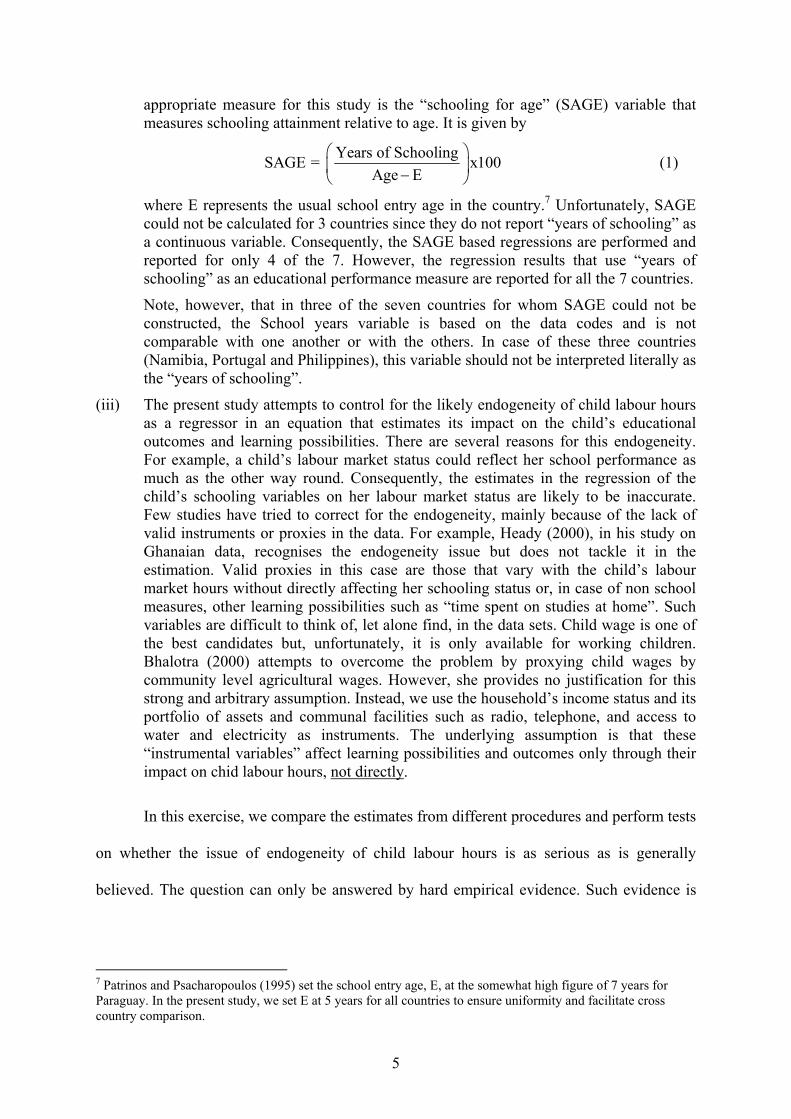
appropriate measure for this study is the “schooling for age” (SAGE) variable that measures schooling attainment relative to age. It is given by

Years of SchoolingSAGE = x100Age E

−

(1)

where E represents the usual school entry age in the country.7 Unfortunately, SAGE could not be calculated for 3 countries since they do not report “years of schooling” as a continuous variable. Consequently, the SAGE based regressions are performed and reported for only 4 of the 7. However, the regression results that use “years of schooling” as an educational performance measure are reported for all the 7 countries.

Note, however, that in three of the seven countries for whom SAGE could not be constructed, the School years variable is based on the data codes and is not comparable with one another or with the others. In case of these three countries (Namibia, Portugal and Philippines), this variable should not be interpreted literally as the “years of schooling”.

(iii) The present study attempts to control for the likely endogeneity of child labour hours as a regressor in an equation that estimates its impact on the child’s educational outcomes and learning possibilities. There are several reasons for this endogeneity. For example, a child’s labour market status could reflect her school performance as much as the other way round. Consequently, the estimates in the regression of the child’s schooling variables on her labour market status are likely to be inaccurate. Few studies have tried to correct for the endogeneity, mainly because of the lack of valid instruments or proxies in the data. For example, Heady (2000), in his study on Ghanaian data, recognises the endogeneity issue but does not tackle it in the estimation. Valid proxies in this case are those that vary with the child’s labour market hours without directly affecting her schooling status or, in case of non school measures, other learning possibilities such as “time spent on studies at home”. Such variables are difficult to think of, let alone find, in the data sets. Child wage is one of the best candidates but, unfortunately, it is only available for working children. Bhalotra (2000) attempts to overcome the problem by proxying child wages by community level agricultural wages. However, she provides no justification for this strong and arbitrary assumption. Instead, we use the household’s income status and its portfolio of assets and communal facilities such as radio, telephone, and access to water and electricity as instruments. The underlying assumption is that these “instrumental variables” affect learning possibilities and outcomes only through their impact on chid labour hours, not directly.

In this exercise, we compare the estimates from different procedures and perform tests

on whether the issue of endogeneity of child labour hours is as serious as is generally

believed. The question can only be answered by hard empirical evidence. Such evidence is

7 Patrinos and Psacharopoulos (1995) set the school entry age, E, at the somewhat high figure of 7 years for Paraguay. In the present study, we set E at 5 years for all countries to ensure uniformity and facilitate cross country comparison.

6

conspicuous by its absence in the literature.8 From a policy viewpoint, the issue of robustness

of the principal findings on the impact of child labour to its treatment as an endogenous or an

exogenous regressor is of considerable importance. This study will attempt to throw some

light on this issue. We take this a step further by jointly estimating child schooling and child

labour hours as a system of equations. The examination of robustness of the impact of child

labour hours on her schooling to the choice of estimation procedure adds to the policy interest

of this study.

While the primary focus of this study is on the impact of child labour on child

schooling, we also include non child labour variables such as the age and gender of the child,

the number of siblings, the educational levels of the parents as regressors or explanatory

variables in the child schooling regressions. As we report below, some of these, especially the

adults’ educational levels and the household’s access to water and electricity, have

significantly positive affects on the child’s educational experience and outcomes. These

results suggest that controlling a child’s labour market activity is not the only way to enhance

her schooling experience and learning achievement. It is possible to moderate the negative

effects of child labour hours on child schooling by influencing the non child labour variables.

The rest of this paper is organised as follows. Section 2 presents the estimation

methodology adopted in this study. Section 3 describes the chosen data sets and presents, via

Tables and graphs, the salient empirical features that throw light on the principal focus of this

study, namely, the impact of child labour hours on her learning achievement. Section 4

presents and discusses the estimation results. Section 5 presents and discusses Sri Lankan

evidence on the impact of occupational category on the child’s learning. We end on the

concluding note of Section 6.

8 See, for example, the recent survey by Bhalotra and Tzannatos (2002) who discuss the endogeneity issue but do not perform or report on any statistical tests on its significance.

7

2. Estimation Methodology

The econometric analysis of the data sets is based on a 3 part estimation methodology.

A. The study uses the multinomial logit model to estimate the determinants of the household’s decision to put the child in one of four observable states, namely, the child (i) attends school, does not work, (ii) attends school and works, (iii) neither attends school nor works, and (iv) works, does not attend school.

B. The exercise, then, moves on from estimating participation/non participation rates to estimating learning measures with special attention paid to the impact of child labour hours consistent with the principal objective of this study. The single equation estimations initially ignore the endogeneity of child labour hours by using OLS but, then, tackle it by using the instrumental variables (IV) method of estimation. The OLS and IV estimates are compared and the Hausman test for the endogeneity of the child labour hours variables is performed and reported.

C. In the final part, the simultaneity between the Schooling outcomes and child labour hours is recognised by jointly estimating them as a two equation simultaneous equation system, using 3 SLS method of estimation. The IV and 3SLS estimates are compared to establish the robustness or otherwise of the principal qualitative results of this study.

This three part methodology is spelt out in more detail as follows.

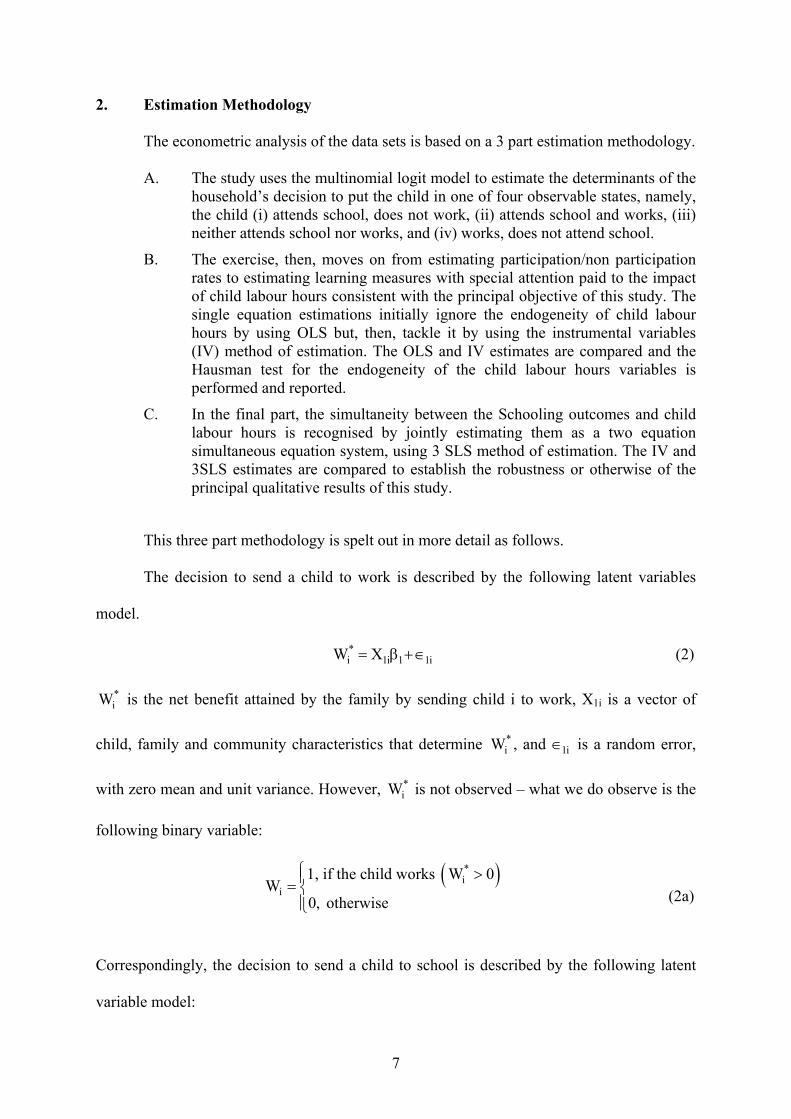
The decision to send a child to work is described by the following latent variables

model.

*i 1i 1 1iW X= β +∈ (2)

*iW is the net benefit attained by the family by sending child i to work, X1i is a vector of

child, family and community characteristics that determine *iW , and 1i∈ is a random error,

with zero mean and unit variance. However, *iW is not observed – what we do observe is the

following binary variable:

( )*

ii

1, if the child works W 0W

0, otherwise

>=

(2a)

Correspondingly, the decision to send a child to school is described by the following latent

variable model:

8

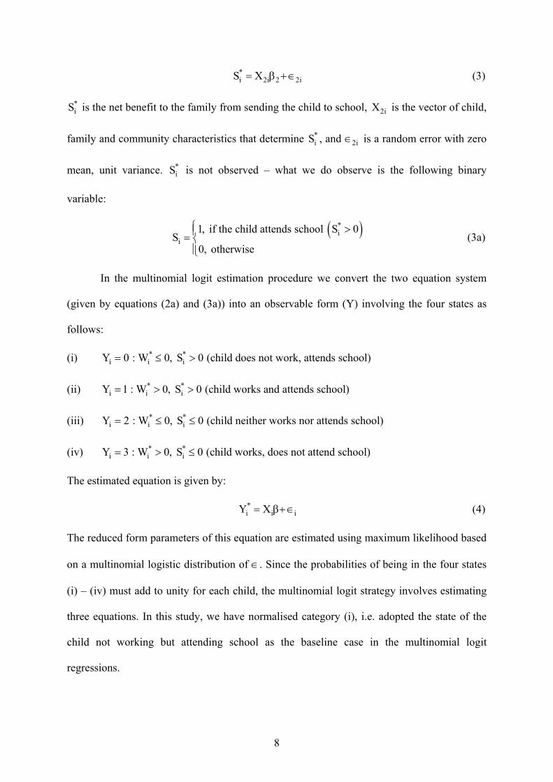
*i 2i 2 2iS X= β +∈ (3)

*iS is the net benefit to the family from sending the child to school, 2iX is the vector of child,

family and community characteristics that determine *iS , and 2i∈ is a random error with zero

mean, unit variance. *iS is not observed – what we do observe is the following binary

variable:

( )*i

i1, if the child attends school S 0

S0, otherwise

>=

(3a)

In the multinomial logit estimation procedure we convert the two equation system

(given by equations (2a) and (3a)) into an observable form (Y) involving the four states as

follows:

(i) * *i i iY 0 : W 0, S 0 (child does not work, attends school)= ≤ >

(ii) * *i i iY 1 : W 0, S 0 (child works and attends school)= > >

(iii) * *i i iY 2 : W 0, S 0 (child neither works nor attends school)= ≤ ≤

(iv) * *i i iY 3 : W 0, S 0 (child works, does not attend school)= > ≤

The estimated equation is given by:

*i i iY X= β+∈ (4)

The reduced form parameters of this equation are estimated using maximum likelihood based

on a multinomial logistic distribution of ∈. Since the probabilities of being in the four states

(i) – (iv) must add to unity for each child, the multinomial logit strategy involves estimating

three equations. In this study, we have normalised category (i), i.e. adopted the state of the

child not working but attending school as the baseline case in the multinomial logit

regressions.

9

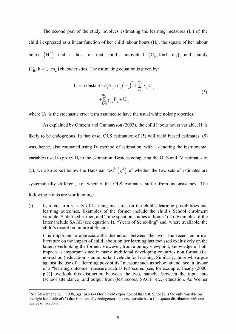
The second part of the study involves estimating the learning measures (Li) of the

child i expressed as a linear function of her child labour hours (Hi), the square of her labour

hours ( )2iH and a host of that child’s individual ( )ik 1C , k 1,., m= and family

( )ik 2F , k 1,., m= characteristics. The estimating equation is given by:

( )

m2 1

i 1 i 2 i 1k ikk 1m2

2k ik 1ik 1

L constant H H C

F U

=

=

= + δ + δ + γ∑

+ γ +∑

(5)

where U1i is the stochastic error term assumed to have the usual white noise properties.

As explained by Orazem and Gunnarsson (2003), the child labour hours variable, Hi is

likely to be endogenous. In that case, OLS estimation of (5) will yield biased estimates. (5)

was, hence, also estimated using IV method of estimation, with Ii denoting the instrumental

variables used to proxy Hi in the estimation. Besides comparing the OLS and IV estimates of

(5), we also report below the Hausman test9 ( )21χ of whether the two sets of estimates are

systematically different, i.e. whether the OLS estimates suffer from inconsistency. The

following points are worth noting:

(i) Li refers to a variety of learning measures on the child’s learning possibilities and learning outcomes. Examples of the former include the child’s School enrolment variable, S, defined earlier, and “time spent on studies at home” (Ti). Examples of the latter include SAGE (see equation 1), “Years of Schooling” and, where available, the child’s record on failure at School.

It is important to appreciate the distinction between the two. The recent empirical literature on the impact of child labour on her learning has focussed exclusively on the latter, overlooking the former. However, from a policy viewpoint, knowledge of both impacts is important since in many traditional developing countries non formal (i.e. non school) education is an important vehicle for learning. Similarly, those who argue against the use of a “learning possibility” measure such as school attendance in favour of a “learning outcome” measure such as test scores [see, for example, Heady (2000, p.2)] overlook this distinction between the two, namely, between the input into (school attendance) and output from (test scores, SAGE, etc.) education. As Weiner

9 See Stewart and Gill (1998, pgs. 142-144) for a lucid exposition of this test. Since Hi is the only variable on the right hand side of (5) that is potentially endogenous, the test statistic has a Chi square distribution with one degree of freedom.

10

(1991) argues in his classic work on South Asian child labour, the immediate cost of child labour is that the child is kept away from school. A child’s school attendance ought to be the first step in the political agenda and, only then, does the impact of child labour on outcomes such as SAGE or, more narrowly, “test scores”, acquire any policy significance.10

(ii) The inclusion of both the child labour hours variable (Hi) and its square ( )2iH is

designed to allow and test for the possibility that the impact of labour hours on the learning measure, Li, changes direction beyond a certain critical value of child labour hours ( )*

iH . That possibility exists if, as we generally observe in the estimations,

1 2ˆ ˆ and δ δ are each statistically significant and have reverse sign. In that case, the

critical value of child labour hours, *iH , at which its impact on the learning measure

reverses direction, is given by

* 1

2

ˆH ˆ2

δ= −

δ (6)

where 1 2ˆ ˆ,δ δ are the estimated values.

(iii) Another measure, which is of policy interest in the present context, is the marginal rate of substitution (φk) between the child’s labour hours and her individual or family characteristics, k, that keeps the child’s learning measure unchanged. φk denotes the change in attribute k that will neutralise the harmful effects of an extra hour of child labour, keeping the value of the child’s learning measure unchanged. From (5), it is easily checked that kφ is given by:

kk

1 2

ˆˆ ˆ2 H

γφ = −

δ + δ (7)

where kγ is the estimated co efficient of attribute k in the equation (5). At the initial point of child’s entry into the labour market, (i.e. when H=0), (7) yields:

kk

1

ˆˆγ

φ = −δ

(8)

Suppose the attribute k is the educational level of the child’s mother as measured by the years of her schooling. If kγ is positive and significant, as is the case in most of

the estimations, and 1δ is negative (i.e. child labour is harmful at the entry point), then

( )k 0φ > denotes the increase in the years of the mother’s education that is needed to cancel out the adverse learning consequences of the first hour of her child’s labour.

Since φk will be dependent on the units of measurement of child labour hours (e.g. weekly or daily hours) and of attribute k, for comparability between countries, it is better to express the child learning compensated interaction between child labour hours and attribute k in terms of elasticity, kφ , as follows:

10 This was recognised, for example, in India where primary schooling for all children was adopted as a goal soon after her independence.

11

k kk

1 2

ˆ Aˆ ˆ H2 H

γφ = − ⋅

δ + δ (9)

where kH,A denote, respectively, the levels of child labour hours and of attribute Ak

at which the elasticity is being calculated. kφ , which is invariant to units of measurement, will denote the percentage change (positive or negative) in attribute k that will be needed to exactly counteract the learning impact of a 1% increase in child labour hours, so as to keep the child’s learning measure unchanged.

(iv) The successful IV estimation of (5) requires the availability of instrumental variables (Ii) in the data set that can serve as valid instruments for the potentially endogenous labour hours variable, Hi.11 Valid instruments are those that (a) are not in the list of predetermined variables that appear in (5), and (b) influence Hi but do not directly influence Li. In the estimations reported below, we have used the household’s access to water and electricity, and its ownership of radio, phone, etc. as instruments. The reader needs to keep in mind that the evidence from the IV estimations is conditional on the validity of the instruments used here.

In the final set of estimations, the study estimates (Li, Hi) jointly as a set of

simultaneous equations, consisting of (5), and the child labour hours equation (Hi) expressed

as a linear function of the child’s individual (Cik) her family characteristics (Fik) and the

instrumental variables (Iik) that were previously used in the IV estimations.

mm m 31 2

i 1k ik 2k ik 3k ik 2ik 1 k 1 k 1H constant C F I U

= = == + ψ + Ψ + Ψ +∑ ∑ ∑ (10)

The 3 SLS estimation used in the systems estimation allows for a non diagonal covariance

matrix, Ω, between the errors (U1, U2) in the two equations (5) and (10). An obvious rationale

for this possibility is the presence of a common set of omitted variables from both equations

that will introduce correlation between the two errors. Note that the 3SLS estimations were

performed and reported for only the 4 countries for which the SAGE variable could be

constructed.

11 The situation is complicated by the presence in (5) of H2 which needs to be instrumented as well. We ignore this complication in the present estimations.

12

3. Data Sets and their Salient Features

In calculating the child’s labour hours, the study uses the standard ILO definition of

child work, including work provided on the labour market and work for household farms and

enterprises, even if it is unpaid. In the case of some of the countries for which such data is

available we include, additionally and separately from the “child labour hours” variable, the

hours spent by the child on household chores as a variable called “domestic hours”. While

there is mounting evidence on the adverse impact of the ILO defined “child work” on

learning, there is very little evidence on the impact of domestic duties. Since such duties can

be quite significant for girls in some societies, a comparison of the impact of the two types of

child labour is of considerable policy significance.

The present study is based on an analysis of the child labour data sets of the following

7 countries: Belize, Cambodia, Namibia, Panama, Philippines, Portugal and Sri Lanka.

Several of these data sets were collected under the ILO’s Statistical Information and

Monitoring Programme on Child Labour (SIMPOC). SIMPOC provides technical assistance

to ILO member States to generate reliable, comparable and comprehensive data in all its

forms. SIMPOC was launched in 1998 in response to the growing need for more

comprehensive statistics on child labour.

The Belize Child Labour Survey is aimed at obtaining information on households

with children between the ages of 5 and 17 years. The Central Statistical Office in Belize

embarked on a study of 6000 randomly selected households and examined in detail the

activities of children aged 5 to 17 years who are found in these households. The Panama data

came from Child Labour Survey 2003, conducted by the Ministry of Labour and Labour

Development, State Treasury Inspector’s Office in collaboration with IPEC, ILO. The Survey

registered 755,032 children between the age of 5 and 17, representing 37.8 percent of the

total population in households with children of that age. In urban areas they constituted 36.5

13

percent of total population, 39.8 percent in rural areas and 40.6 percent in indigenous areas.

The Cambodian data was obtained from the Cambodia Child Labour Survey, 2001. The

sampling plan, the survey schedule, the tabulation plan etc. of the survey were prepared in

consultation with ILO’s SIMPOC. The survey covered a sample of 12,000 households, which

were interviewed on the nature of the economic activities of each child within the household,

the consequences and challenges faced by each child while in employment, and the amount

of time the child spent for his/her studies and recreational activities as well as on economic

activities and household chores. The Portuguese data came from the Child Labour in Portugal

survey in 1998. This first time child labour estimation project in Portugal (phase one of three

planned phases) was carried out in October 1998, with a questionnaire being conducted of

families in mainland Portugal. Unlike most SIMPOC surveys, the Portugal survey was

funded by the country, and only the technical assistance was provided by IPEC/SIMPOC.

The age group covered in the Portuguese study was children aged 6 to 15 years. The

Namibian data came from the National Child Activities Survey (NCAS) which was

conducted on a sample basis covering the whole country in February/March 1999. The target

group for this survey was the population of children aged 6 to 18 years, in accordance with

the UN definition of a child and the official definition of the schooling age in Namibia. The

objective of NCAS was to provide base line data on the activities of the child population in

Namibia for planning purposes, policy implementation and monitoring and the evaluation of

government development programmes aimed at improving the status of the vulnerable socio-

economic groups of the Namibian child population. The Philippines data came from the

survey undertaken by the National Statistics Office there in close collaboration with the

Bureau of Labour Employment Statistics of the Department of Labour and Employment. The

urban and rural areas of each province were the principal domains of the survey. The sample

included approximately 25500 households nationwide. All children aged 5 to 17 years old

14

who were found to have worked at any time during the past twelve months at the time of the

survey (August, 1994 – July 1995) were interviewed. Survey questionnaires were directed to

household head as well as at the child. The Sri Lankan data came from the Child Activity

Survey, Sri Lanka, 1999. The sampling plan, the survey schedule, the tabulation plan, etc. of

the survey were prepared in consultation with the ILO, Bureau of Statistics. The survey

covered a sample of 14400 households, which were interviewed on the nature of the

economic activities of each child within the household, the consequences and challenges

faced by each child while in employment, and the amount of time the child spent for his/her

studies and recreational activities.

Table 1 presents some relevant summary statistics (at sample mean) for the seven data

sets, disaggregated by the gender of the child. Note that while not all the information is

available for all the seven countries, the only variables that are fully comparable across all the

countries are: the mean age of the child in the sample, the current school attendance rates, and

their disaggregation between the four mutually exclusive combinations of the child’s

participation/non participation in schooling and in employment.12 Moreover, the SAGE

variable [see equation (1)] is comparable between the four countries for which this measure

of learning outcome could be constructed. The following remarks may be noted:

(i) The current school attendance rate varies a good deal between the chosen countries – from the low rates of Namibia to the more satisfactory rates of Portugal and Sri Lanka. Inspection of the rates of schooling/employment combinations shows that they vary a good deal more between the countries – for example, between the low rate of 28.5% for purely school enrolled girls in Cambodia to the high rate of 96.1% in case of Portuguese girls. In the Asian countries, Cambodia, Philippines and Sri Lanka, a much greater percentage of children combine schooling with employment than in the other countries.

(ii) There are several instances of gender differential between boys and girls in the data though we do not detect any uniform patterns. In Belize and Sri Lanka, for example, boys work longer hours than girls on ILO defined child work but girls work longer hours on household chores or domestic duties. The latter is the case for all the countries for which information on domestic hours is available.

12 See Appendix A (Table A1) for the child gender differentiated rates calculated separately for the age groups 12, 13 and 14 years.

15

(iii) Of the 4 countries for which SAGE is available, Sri Lankan children record the best schooling outcome. It is disappointing to note that children in the age group 12-14 years in Belize, Cambodia and Panama lag so far behind the Sri Lankan children. Alternatively, the Sri Lankan performance is quite impressive keeping in mind its status as a poor, developing country. It is interesting to note that, on either measure of “school outcome”, girls do better than boys in all the countries.

(iv) The weekly work hours vary a good deal between the comparable countries. Note, incidentally, that while the Sri Lankan figures on domestic duties are in “minutes a day”, the ILO definition based child work hours figures for Belize are in terms of “hours a day”. All the other work figures are weekly and comparable between countries. Working children in the age group 12-14 years in Sri Lanka work considerably fewer hours than their counterpart in the other countries. The weekly child labour hours in Namibia and Panama exceed those in Sri Lanka by a factor of more than two to one. Notwithstanding Portugal’s status as a developed country and a satisfactory school attendance rate that is consistent with this status, Portuguese working children in the age group 12-14 years record quite high weekly work hours.

(v) Another feature that is worth noting is that domestic duties constitute a significant share of the child’s total work load. For example, in the case of Cambodia and Portugal, on average a working child spends, respectively, (approximately) 35.40% and 27.58% of her/his total working hours on domestic duties. In the 4 countries for which information on domestic duties is available, girls generally work longer domestic hours than boys. Nowhere is this gender differential as strikingly high as in Sri Lanka. This has, however, not prevented the school enrolment rates in Sri Lanka from being virtually the same for boys and girls. The significant hours that children in the age group, 12-14 years work on domestic duties underline the need for empirical evidence, provided later in this paper, on the impact of domestic hours on the child’s learning.

Figures 1(a) – 7(a) plot, for the seven data sets, the graphs of the mean current school

attendance rate on the y-axis against the weekly work hours (daily in case of Belize) of the

working child on the x-axis. Note that since these graphs are based only on the observations

on working children in the age group 12-14 years, the sample size falls sharply as the

working hours increase. Hence, these relationships, especially in the middle to upper range of

labour hours, should not be taken too literally. Figures 1(b) – 7(b) plot the corresponding

graphs of the school outcome variable, SAGE (wherever available) and “years of schooling”

(for the others) against work hours. It is clear from these graphs that work hours do adversely

affect both school enrolment rates and the school outcome variable. However, the shape of

these relationships vary between the countries. For example, in case of Namibia and Sri

Lanka, the first few child labour hors do not seem to have much of an adverse impact on

16

either school attendance or the school outcome, unlike in Belize where they do. However, all

the data sets agree on the damage that long work hours inflict on a child’s learning

experience.

We have alternative and additional evidence on the adverse impact of child labour on

the child’s learning possibilities. Figure 8(a) shows the relationship between study time (at

mean) and the child age for non working and working children in Sri Lanka. The mean study

time of working children falls below that of non working children around 11 years. The

decline accelerates over the age group 12-14 years considered here so that by the time a child

reaches school leaving age a large gap opens up between the mean study time of non working

and working children. Figure 8(b) shows the corresponding relationships for only children in

Sri Lanka who attend school. It is interesting to note that though non working children

continue to enjoy higher study time than working children in the later age groups, the mean

study time increases with child age for both groups of children, unlike in the previous figure.

The suggests that work combined with schooling is less harmful to the child’s learning

possibilities than work which is at the expense of schooling. Figure 9 shows, separately for

working and non working children in Cambodia, the percentages of children in the various

age groups who can read and write. Once again, the cost of child work is evident in the higher

percentages that non working children enjoy over working children in reading and writing

literacy, in the target age group, 12-14 years, of this study.

The results of this section provide prima facie evidence on the damage caused to the

child’s learning by child labour. However, the summary measures provided here do not

provide any clear evidence on the impact of child labour hours on human capital

accumulation since they do not control for the other variables. To get a clearer picture, we

turn to the results of estimation in the following section.

17

4. Estimation Results

We present and discuss the estimation results of the seven countries in alphabetical

order beginning with Belize. Table 2 presents the results of the multinomial logit estimation

of equations (2a, 3a) with the category of children who attend school but do not work being

adopted as the normalised category. Note that the estimate of the constant term, which was

included in all the regressions, has not been presented in the Tables. The sign of the estimated

coefficient shows the direction of change in the probability of a child aged 12-14 years being

in that category, relative to the normalised category, if the determinant goes up by 1 unit. Of

particular interest in the present context is the estimated coefficient of the “years of

schooling” variable. The negative and significant coefficient estimates of this variable in

categories 3 and 4 suggest that an increase in the years of schooling pushes children from

these categories into category 1. In other words, school attendance can be “habit forming” in

the sense that, ceteris paribus, the more schooling experience a child gets the less likely that

she/he will drop out of school. An increase in the household’s access to water and light and in

its possession of assets such as television and telephone helps to put its children in category

1, i.e. a “school only” status with no labour market participation.

The marginal probabilities, implied by the multinomial logit parameter estimates of

Belize presented in Table 2, are reported in Appendix A (Table A2). These are easier to

interpret than the multinomial logit parameter estimates. The marginal probabilities in Table

A2 show that boys in Belize are less likely than girls to be in the “school only” category and

more likely to be in the “work only” category. This is explained by the fact that “work” does

not include domestic duties. The marginal probabilities also confirm that access to lighting,

water, etc. encourages the household to put its children in the “school only” category. The

base probabilities show that, free from the influences of the various explanatory variables

18

listed in Table A2, a child in Belize is much more likely to be in the “school only” category

than in the other categories.

Tables 3, 4 and 5 present the results of OLS and IV estimation of the child’s school

enrolment status, “years of schooling” and SAGE, respectively, in Belize on a select set of

determinants. The Wu-Hausman statistics confirm that in case of all these three dependent

variables the OLS estimates for Belize are inconsistent. The result is conditional on the

validity of the instruments used here. The IV estimates show that, ceteris paribus, boys enjoy

superior school enrolment rates than girls but not on the “years of schooling” or SAGE

criterion.

On the principal focus of this study, the IV estimates show that work hours adversely

affect both school enrolment (i.e. the probability of the child attending school) and the school

outcome variables from the first hour itself. However, the estimated positive coefficient of

the work hours square variable suggests that the adverse marginal impact of child labour

hours on the schooling variables weaken as the labour hours increase. The IV regressions

agree that beyond 5 hours a day the marginal impact changes direction, i.e. child labour hours

impact positively on her school enrolment and the measures of school outcome. Note,

incidentally, that the OLS coefficient estimates of the work hours variables, because of the

inconsistency, yield quite different qualitative results from the IV estimates. The gender

disaggregated IV estimates of the “years of schooling” equation for boys and girls in Belize,

presented in Table 6, yield a similar picture. It is interesting to note that the turning point

where the incremental impact of child labour hours on schooling years changes direction is

remarkably robust – 4.37 hours a day for boys, 4.51 hours for girls and 4.40 hours for all

children. The turning points for the impact of labour hours on school attendance is 4.65

hours, and on the SAGE measure is 4.39 hours. Note, however, that as the Belize data

analysis shows, these turning points will rarely be reached since very few children will clock

19

such high work hours. The point to note from the Belize evidence is that the disutility to the

child from the first labour hour as she starts working is quite high. For example, the first hour

of child labour reduces the probability of the child’s school attendance by approximately

50%.13 Alternatively, it leads to a reduction in the “years of schooling” by 2.569 years. The

gender differential is quite noticeable – the reduction in the years of schooling of boys is 2.13

years while that of girls is 3.69 years. It is mildly reassuring that the marginal impact

weakens with each additional hour that the child works, but it will take absurdly long

working hours for the marginal adverse effects on learning to disappear altogether. To

examine whether these results are robust to the data set, let us now turn to the Cambodian

regressions.

The multinomial logit estimation results for Cambodia are presented in Table 7. The

results are similar in several respects to those of Belize presented in Table 2. Note the strong

role that parental educational levels, the household’s possession of assets such as TV, phone,

etc. and its access to amenities such as light and water play in encouraging its children to stay

in school. The marginal probabilities for Cambodia are presented in Appendix A (Table A3).

These show the strong role that adult education plays in pushing children into the “school

only” category. A comparison of the base probabilities in the Appendix A Tables A2, A3

shows that Cambodian children are much more likely to combine schooling with employment

than children in Belize. This is consistent with the picture presented in Table 1.

Tables 8-11 present the OLS and IV estimates of, respectively, the Cambodian child’s

school enrolment status, years of schooling, SAGE and ability to read or write variables

regressed on a selected list of determinants. In keeping with the chief motivation of this

study, we focus our attention on the impact of child labour hours on the school attendance

and school outcome measures mentioned above. Unlike in the Belize case, the IV estimates 13 This figure and the ones mentioned below were obtained by calculating

1 2ˆ ˆ2δ + δ where

1 2ˆ ˆ,δ δ are the

estimated coefficients of labour hours and (labour hours)2 in the relevant regressions.

20

of the school enrolment equation are not statistically significantly different form the OLS

estimates, as the Wu-Hausman statistics confirm. This is however not true of the school

outcome regression equation estimates (Tables 9, 10). Also, unlike in Belize, the IV estimates

do not find the work hours impact on current school attendance to be significant. In contrast,

rising levels of adult education in the household have very strong impact on the child’s

school enrolment. Tables 9, 10 confirm, via the IV coefficient estimates of the work hours

and (work hours)2 variables, that child labour does impact quite negatively on the principal

alternative learning measures, namely, “years of schooling” and SAGE, though this adverse

impact weakens with each additional hour worked over the week by the child. For example,

at the entry point to the labour market, the first hour worked over the week by the child

reduces her/his “years of schooling” by 0.30 of a year.14 It is interesting to note that the

turning point of the U shaped relationships occurs at approximately 30 hours per week which

is consistent with the figure of approximately 4.50 hours a day that we reported for Belize.

Table 11 reports that child labour, also, impacts negatively on the child’s ability to read or

write. While the IV estimates show that this impact is only weakly significant, the OLS

estimates register higher levels of significance. However, the magnitudes of the coefficients

of the linear and quadratic child labour hour variables are so small that the damage caused by

child labour to the child’s ability to read and write is of a negligible order of magnitude. The

gender disaggregated regression estimates of the SAGE equation, presented in Table 12, yield

a picture which is quite similar to that implied by Table 10, namely, that for boys and girls,

labour hours initially impact negatively and non linearly on SAGE and that the turning points

for the U shaped relationship between SAGE and child labour hours occurs around 28-30

hours a week for both boys and girls.

14 Note that the magnitudes of the labour hour coefficients in Cambodia and Belize are not directly comparable since, while the Cambodian child hour figures are on a weekly basis, those in Belize are daily figures.

21

Let us now turn to the results of Namibia. To concentrate our minds on the principal

objective of this study which is on the impact of child labour hours on her learning, we do not

present the results of the multinomial logit estimations for Namibia and the remaining

countries. However, those estimates will be made available on request. Table 13-15 present

the OLS and IV regression estimates of the Namibian child’s school enrolment status, years

of schooling and read/write ability, respectively, as a linear function of the select list of

determinants. In case of the read/write equation (Table 15), while the OLS estimates15

provide evidence of statistically significant negative impact of the child’s literacy status,

there is no such evidence in the IV results. This is consistent with the Cambodian results

presented and discussed above. Note that the regressions were performed on the target group

of 12-14 year old children. Since a child’s literacy status is established by the time she/he

reaches this age group, this result simply confirms that child labour does not significantly

alter the literacy status of this older group of children. We expect the adverse impact, if any,

of child labour on the read/write variable to be felt by the younger children in the sample.

This issue can be investigated by running regressions on, say, 5-8 year old children in the

sample.

The IV estimates of Tables 13, 14 do not provide convincing evidence of any negative

impact of child labour hours on either school enrolment or years of schooling in Namibia.

The Namibian results are inconsistent with much of the above evidence. Note, however, from

the gender disaggregated regression estimates of the “years of schooling” variable presented

in Table 16, Namibian boys seem to experience stronger negative impact (in both size and

significance) than Namibian girls of child labour hours on the measure of school outcome.

Note, also, from Tables 13 and 14 that the OLS estimates provide much stronger evidence of

the adverse impact of child labour hours on the child’s learning for the target group of 12-14 15 It might be argued that the OLS estimates should be taken more seriously than the IV estimates in case of the read/write regressions, since there is unlikely to be any reverse causation between the literacy status and labour hours of a child in 12-14 year age group.

22

year old children that have been considered in this study. The validity of the instruments,

used here, has not been tested in this study. Consequently, the IV results should not

necessarily be considered to be more reliable than the OLS ones. As Hoddinott and Kinsey

(2001) report in the context of child health, with poorly chosen instruments, the bias found in

2SLS or 3SLS estimates is as large as that found in the OLS results. The issue merits a

separate investigation on the sensitivity of the regression results to different selections of

instruments, calculation of the Sargan tests for validity of instruments [see Stewart and Gill

(1998, pgs. 135-144)], etc. Such an investigation is best left for a separate exercise.

Turning now to Panama, Tables 17-19 present, respectively, the estimates of the

school enrolment status, years of schooling and SAGE regressions of Panamian children in

the age group 12-14 years. Table 20 presents the gender disaggregated estimates of the SAGE

regressions of children. The results are in line with previous evidence that suggests that child

labour impacts negatively on the child’s learning, though the magnitude of the negative

marginal impact weakens with each additional labour hour that the child works. The turning

point for the U shaped relationship between the child’s labour hours and her learning occurs

around 30 hours a week which is in the range witnessed earlier in the Cambodian regressions.

Note from the gender disaggregated estimates of the SAGE regressions presented in Table 20

that, on both OLS and IV results, the negative impact of child labour hours on learning is

much higher for girls than for boys in Panama. However, the IV estimates show that the

turning point is earlier for girls (25.06 weekly labour hours) than for boys (30.38 weekly

labour hours). Note that, of the other determinants, the level of both adult male and adult

female education plays a strong role in improving the child’s educational performance.

Turning to Philippines, let us note that, due to lack of the relevant identifying variable

in the data, we were unable to link the information on the child with the household

characteristics of that child. Consequently, the regressions for Philippines did not include

23

household level variables. While Tables 21, 22 present the regression estimates of school

enrolment and the “years of schooling” variables, Table 23 presents the corresponding gender

disaggregated estimates of the latter. The results are supportive of the previous evidence of a

U shaped impact of child labour hours on years of schooling of the child. The turning point

occurs at 34.19 weekly hours for all children, 33.35 weekly hours for boys and 36.15 weekly

hours for girls. These turning points occur somewhat later than what was observed

previously. This may be the consequence of our failure to include the household level

variables in the Philippine regressions, unlike for the other country data sets, due to the lack

of the relevant identifying code in the data. Note, incidentally, that in contrast to the

Panamian evidence, the negative impact of child labour hours on the years of schooling of the

child is much smaller (in both size and significance) for girls than for boys.

Tables 24-27 present the evidence for Portugal. Tables 24, 25 present, respectively,

the regression equation estimates of the school enrolment status and the “years of schooling”.

Table 26 presents the gender disaggregated regression estimates of the latter. Table 27

presents the Portuguese evidence on the impact of child labour hours on the number of

failures of school children in the age group 12-14 years. The latter is probably the most

satisfactory measure to use in assessing the impact of child labour hours on the educational

performance of high school children. The Portuguese data set provides a distinctive and

useful set of information in this regard. The results are generally consistent with the idea of a

U shaped relationship between learning outcome and child labour hours among children in

the target age group 12-14 years. A significant exception is provided by the regression

estimates of the “years of schooling” received by Portuguese girls. Their estimates point to an

inverted U shaped relationship rather than a U shaped one. Table 27 confirms that a ceteris

paribus unit increase in the child labour hours leads to a worsening of the child’s school

performance that is reflected in a 0.34 increase in the failure rate. The effect flattens out at a

24

weekly level of 26.27 child labour hours. Another useful piece of evidence that the

Portuguese results provide is on the impact of domestic hours on the child’s learning. The IV

estimates show that, similar to the ILO defined child labour hours, domestic hours impact

negatively on learning by significantly reducing the school enrolment and the years of

schooling received by the child and by increasing the number of failures that the child

experiences at high school. However, the magnitude of the adverse impact of domestic hours

on learning is generally less than that of market hours.

Let us now turn to the Sri Lankan results. Sri Lanka is quite unique in the sense that,

not withstanding its status as a developing country, it does quite well on several indicators of

human development approaching the rates of developed countries [see, for example, Sen

(1999)]. As Table 1 shows, Sri Lanka has a school attendance rate of 94% which is only

marginally below that of a developed European country such as Portugal. Hence, the Sri

Lankan evidence should be of particular interest for this study. Tables 28-32 contain the Sri

Lankan results. The impact of child labour hours on the child’s current school attendance

status, years of school, the child’s study time, SAGE and the gender disaggregated estimates

of the latter are presented in Tables 28-32, respectively. The estimates show that the Sri

Lankan results on the impact of child labour hours on the child’s learning outcomes (as

measured by SAGE, for example) and learning possibilities (as measured by the child’s study

time) is at odds with much of the previous evidence. The coefficient estimate of the work

hours variable is positive and significant while that of its square term is significantly negative

thus suggesting an inverted U shaped relationship in Sri Lanka between the child’s labour

hours and her/his learning unlike much of the evidence for the other countries presented

above. In other words, small amount of child labour is actually quite beneficial to the child’s

learning in Sri Lanka. Table 32 confirms that this result is true of both boys and girls and

holds for both the OLS and the IV estimates. The SAGE estimates imply that the turning

25

point, i.e. the point at which child labour starts to impact negatively on learning, is 18.785

labour hours per week for boys and 14.167 labour hours per week for girls. The Sri Lankan

experience is, also, evident from the graphs [Figures 7(a), 7(b)] and the summary statistics

which show that the child’s learning measure do not register a significant decline until child

labour hours register weekly levels of 15 hours or more. Of course, the fact that a large

workload does impact negatively on learning is, also, clear from the graphs, especially of the

School attendance rate, which falls sharply at high levels of work hours. The fact that a

sizeable section of the Sri Lankan child labour force works less than 17.85 hours a week,

which is the turning point implied for all children by the SAGE regression estimates of Table

31, suggests that child labour is less destructive of the child’s development in Sri Lanka than

in other countries. We do not have any ready explanation of this puzzling but interesting

result. One possible explanation is that, as Table 1 shows, relatively fewer Sri Lankan

children are in the “work only” category than in the other developing countries. Alternatively,

a greater percentage of the child force in Sri Lanka combine schooling with employment than

in other developing countries.16 This helps to ameliorate, at moderate levels of work hours,

the harmful effects of child labour. This result merits further investigation as it is of

significant policy interest.

One result that all the data sets agree on is the strong positive role that the level of

adult education in the household plays in keeping the child enrolled in school and in

improving her learning performance. The paper has earlier introduced, via equation (9), an

elasticity measure kφ that calculates the percentage change in the level of adult education

that will exactly counteract the damage to learning caused by a 1% marginal increase in child

labour hours. Table 33 reports the IV based illustrative estimates of kφ for Cambodia and

16 See Ray (2000a) for similar evidence on difference in the nature of child labour between Peru and Pakistan. Children in Peru combine schooling with employment far more than in Pakistan.

26

Panama calculated at the mean levels of child labour hours and adult education levels in these

countries. In Panama, for example, a 0.54% increase in adult male education is needed to

counteract the harmful effect of a 1% increase in the child labour hours of boys, compared to

a figure of 1.22% for Panamian girls. The estimates in Table 33 suggest that a much higher

percentage change in adult education levels is needed in Panama than in Cambodia to

counteract the harmful effects of child labour on the child’s learning. The gender differential

between boys and girls reverses itself between the two countries. Note, however, that in both

countries adult female education levels needs to increase by a higher percentage than adult

male education levels to counteract the harmful effects of a 1% increase in child labour hours.

The estimates of the school outcome (Li) and labour hours (Hi) equations [equations

(5) and (10)], estimated as a system of equations using 3SLS, are presented in Table 34. For

clarity of presentation, we have only reported the 3SLS estimates of the SAGE (Li) equation.

for the 4 countries (Belize, Cambodia, Panama and Sri Lanka) for which SAGE could be

constructed and compared. The 3SLS estimates of the child labour hours (Hi) equation will be

available on request. Since the child labour hours are daily figures for Belize and weekly for

others, the labour hour coefficients in Belize are not comparable with those in the other

countries. The following points are worth noting:

(i) Ceteris paribus, boys complete significantly less years of schooling than girls, on the age corrected measure of schooling, in Cambodia and Sri Lanka. In contrast, no significant gender differential exists in Belize or Panama. The former result can, also, be contrasted with the evidence, based on test scores, presented in Heady (2000), for Ghana where girls perform worse than boys.

(ii) Sri Lanka’s isolated example as the only country in our data set where child’s work hours initially impact positively on the child’s learning is reaffirmed by the 3SLS estimates. The inverted U shaped relationship between the child’s learning and her/his work hours in Sri Lanka reverses to a U shaped relationship in case of the other countries. The turning points are 13.55 weekly hours in Sri Lanka, 4.96 daily hours in Belize, 41.38 weekly hours in Cambodia and 37.52 weekly hours in Panama17. The turning point for Sri Lanka, unlike in the others, is more than of academic interest

17 These estimates do not disaggregate the working children between the various occupation categories. Such disaggregation was subsequently performed for Philippines and Sri Lanka and the results incorporating the occupation specific affects are presented in Appendix B (Philippines) and Section 5 (Sri Lanka)

27

since a significant number of the child workers work in the range of 0-15 weekly hours. Consequently, a much greater percentage of child workers in Sri Lanka is on the upward rising segment of the relationship between child learning and child labour hours than in the other countries.

(iii) In contrast to the ILO defined child work hours used here, hours spent by the child on domestic duties impact negatively on learning in Sri Lanka but less significantly in Belize, the other country for which data on domestic hours is available in the data set. It is interesting to contrast this with the Cambodian experience which suggests the reverse, i.e. domestic hours increase the child’s schooling experience.

(iv) There is general agreement that rising levels of adult education promote child welfare by reducing the child’s work hours and by increasing the SAGE measure of school outcome of that child. In all the four countries, reported in Table 34, adult female education levels exert a stronger impact than adult male education on the child’s learning. In this and other key respects, the qualitative results are reasonably robust between the OLS, IV and 3 SLS results. Note, also, from Table 34, that there is general agreement between the four countries that an increase in the number of children in the household adversely affects the learning outcomes of the child.

With the exception of Belize, all the 3 SLS estimates of Table 34 are based on the

weekly hours data of child labour. Table 35 reports the corresponding 3 SLS estimates for

Cambodia and Sri Lanka based on daily hourly data for child labour. The Sri Lankan

regression estimates are reported both when one controls for the days worked per week and

when one doesn’t. Tables 34, 35 agree on the qualitative difference between the Cambodian

and Sri Lankan estimates. Child labour impacts negatively on the child’s schooling in

Cambodia right from the first hour of her/his employment. In contrast, child labour impacts

negatively on the schooling in Sri Lanka only beyond 3-4 hours of child work a day. Table 35

also shows that, ceteris paribus, an increase in child labour due to an increase in the number

of days worked by the child in the week, can have a sharply negative impact on the child’s

schooling experience. The policy implication of this result is that, to minimise the negative

impact of child labour on the child’s education, it is better to control, first, the number of days

in the week the child works rather than the length of the working day.

28

5. Impact of Occupational Category on the Child’s Learning: the Sri Lankan

Evidence

We extend the discussion on the implication of disaggregation of the employed

children by their occupational categories for the estimated relationships to the case of Sri

Lanka. Table 36 presents the mean values of school enrolment rates, SAGE and study time

for Sri Lankan child labourers in the age group 12-14 years, disaggregated by the following 4

occupation categories: (i) Service workers, Shop and Market sales workers (ii) Craft and

related workers (iii) Sales and services workers in elementary occupations, and (iv)

Agricultural workers. This table also reports, for use as a benchmark, the corresponding mean

values for children who are not working on ILO defined “economic activities”. Similar to the

evidence for Philippines presented in the Appendix (Table B1), the school enrolment rate

shows considerable variation between the four occupational categories, namely, from the low

rate of 39.5% for children employed as sales and services workers in “elementary

occupations” to the high rate of 94.3% experienced by children who are agricultural workers.

Note that the latter rate is only marginally below the school enrolment rate of 96.3% recorded

by the non working children. Note, also, that the school enrolment rate of agricultural child

workers in Sri Lanka (94.3%) is much higher than the comparable rate (78.6%) in the

Philippines presented in Table B1. This is consistent with our earlier remark on the high

aggregate school enrolment rates in Sri Lanka, notwithstanding its status as a developing

country. The age corrected schooling measure, SAGE, varies less than the school enrolment

rates though this variable, along with the mean study time, also registers a substantial drop

for children employed in “elementary occupations”.

Table 37 presents the OLS estimates of the regressions of SAGE (a measure of

learning output) and study time (a measure of learning input) on the various determinants

used earlier (see Tables 30, 31) along with interaction terms between the four occupational

29

dummies and the labour hours, (labour hours)2 variables. Focussing initially on the estimated

coefficients of the interaction term involving the labour hours variable, it is clear that in case

of only two of the four occupation categories do the first few hours of employment negatively

impact, in a significant way, the schooling measure, SAGE. Indeed, for agricultural workers,

the impact is significantly positive and, since this category constitutes nearly 20% of the

working children in the age group 12-14 years, it explains the positive coefficient estimate of

the labour hours variable in the aggregate estimations reported in Table 31. The negative

coefficient estimates of the interaction terms between the labour hours square variable and

the occupational dummies reported in Table 37 show that heavy work load does eventually

adversely affect the schooling of children in all the occupation categories. Recalling the

identification of turning point in the relationship between learning and labour hours (see

equation (6)), Table 37 suggests that “light work”, defined as child work that does not

negatively impact on the child’s “capacity to benefit from the instruction received” should

mean a maximum work load of 10.54 hours a week for service workers, shop and market

sales workers and 10.88 hours a week for agricultural workers. These cut off points are

somewhat lower than those suggested by the IV estimates of Tables 29, 31 and 32 which

ignored the occupational disaggregation. While the IV estimates suggest a definition of “light

work” as one involving a maximum work load of 15-18 hours a week, the OLS estimates

imply a maximum workload in the range of 9-11 hours a week. The child gender

disaggregated estimations on Sri Lankan data done in this study (see Table 32) suggest a

lower maximum weekly work load for girls than for boys in defining “light work” as one that

does not negatively impact on schooling. Table 37 shows that, with the significant exception

of child workers in occupation category 3, study time is not much affected by the child labour

hours. Table 38 reports, separately for the four occupation groups, the SAGE regression

estimates for Sri Lanka based on the daily hourly data for child labour. These occupation

30

disaggregated estimates are supportive of the proposition that, in Sri Lanka, “light work”

need not be harmful to the child’s education. This contrasts sharply with the Cambodian

experience.

6. Summary and Conclusion

ILO Convention No. 138, Art 7(b) stipulates that light work may be permitted at the

age of 12 or 13 provided it does not “prejudice attendance at school” nor the “capacity to

benefit from the instruction received”. This raises the question: Does a limited amount of

children work at these ages “prejudice attendance at school” and/or damage the child’s

“capacity to benefit from the instruction received”? Unfortunately, the existing child labour

literature does not provide any definitive answer to this question since: (a) much of it is

concerned with analysing the causes or determinants of child labour rather than its

consequences, especially on human capital, and (b) the few published studies that attempt to

answer this question do not address the issue of endogeneity of child labour hours in the

estimation. The latter follows from the reverse impact, especially intertemporally, of learning

on child labour.

The principal motivation of this study is to answer the above question whose policy

importance can be seen in the context of ILO Convention No. 138. In basing the study on

multi country SIMPOC data sets and in using alternative estimation methods, the exercise

examines the robustness or otherwise of the evidence on the impact of child labour hours on

the child’s school attendance and performance. The central message from this study is that

child work, even in limited amounts, does adversely affect the child’s learning as reflected in

a reduction in the school attendance rate and in the length of schooling received by the child.

The damage done by child work to the child’s learning is further underlined by the adverse

impact of work hours on the child’s ability to read and write in Cambodia (Table 11) and in

Namibia (Table 15), with the latter result holding true only under simplifying estimation

31

assumptions. Further support for the proposition that child work is detrimental to the child’s

learning comes from the result that work hours significantly increase the rate of failures

experienced by the child in Portugal (Table 27).

With one significant exception (Sri Lanka) and a less significant one in Namibia, the

result on the negative impact of child work on her learning is remarkably robust to the data

set, to the gender of the child and to the estimation procedure adopted. On the latter,

controlling for the endogeneity of child labour, seems to worsen its impact on human capital

formation. The gender disaggregated estimates generally suggest that the marginal impact of

child work is more detrimental to the learning experience of girls than boys, though there are

some exceptions to this result. In contrast to the ILO defined child labour hours, the domestic

hours clocked up by the child improves her schooling experience in Cambodia but reduces it

in Sri Lanka. The contrast between the effects of these two types of child work on learning

could not be more marked in these countries.

A significant exception to the result that child work, even in limited amounts,

damages the child’s learning is provided by the Sri Lankan experience. Sri Lanka stands

alone in providing evidence that supports the basis of ILO Convention 138 Art. 7 that at the

ages of 12 and 13, the child can combine work and school in such a way that school

performance does not suffer. The Sri Lankan results suggest that a child in the target age

group 12-14 years that is considered here can work up to somewhere between 12-15 hours a

week without suffering a loss in her school attendance rate or in the length of her schooling.

While the former result is true only of one set of estimates (Table 28), the latter result is true

under all estimation procedures (Tables 31, 34). Another reason to take this latter result

seriously is provided by the fact that it holds true of both boys and girls in Sri Lanka as the

gender disaggregated estimates of Table 32 show. We have no ready explanation as to why

Sri Lanka stands alone in this respect besides noting that, notwithstanding its status as a

32

developing country; Sri Lanka approaches the school attendance rates of developed countries

such as Portugal (Table 1). Note, incidentally, that even in Sri Lanka the child’s school

performance deteriorates sharply at high work hours.

Though the focus of this study is on the impact of child work on the child’s learning,

there are other features of our results that deserve special mention. In general, boys fare

worse than girls on the length of their schooling (Table 1). Children in female headed

households and in households with low levels of adult education tend to perform worse than

other children. The result on the strong positive impact of adult education on the child’s

schooling variables holds true for all the data sets and is robust to the estimation method. The

Portuguese and Sri Lankan results drive home the importance of adult education for the

child’s learning by providing evidence that suggests that increases in the adult education

levels reduce the number of failures experienced by the child in Portugal (Table 7) and

increases the child’s study time in Sri Lanka (Table 30).

There is a policy message in the result on the strong and positive role that adult

education plays in improving the child’s learning. If some “light work” is permitted for

children in the ages of 12 and 13 years, as suggested in ILO Convention 138, Art. 7, then it

should be accompanied by a campaign to improve the adult education levels. Better educated

adults will, by ensuring that their children make more efficient use of the non labour time for

study, will help to reduce the damage done to the child’s learning by her work hours. The

compensated elasticities of substitution between adult education levels and child labour

hours, that keep the child’s schooling unchanged, calculated for Cambodia and Panama

(Table 33) should give the policy makers some idea of the task involved.

Before concluding, let us make as “lessons learnt” a few comments on the seven

SIMPOC data sets used in this study. Much of the existing empirical literature on child labour

has been on the LSMS data sets collected under the auspices of the World Bank. This is one

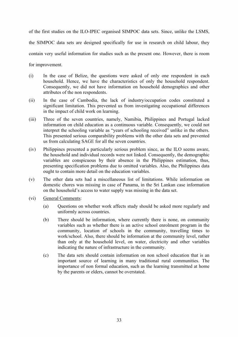
33

of the first studies on the ILO-IPEC organised SIMPOC data sets. Since, unlike the LSMS,

the SIMPOC data sets are designed specifically for use in research on child labour, they

contain very useful information for studies such as the present one. However, there is room

for improvement.

(i) In the case of Belize, the questions were asked of only one respondent in each household. Hence, we have the characteristics of only the household respondent. Consequently, we did not have information on household demographics and other attributes of the non respondents.

(ii) In the case of Cambodia, the lack of industry/occupation codes constituted a significant limitation. This prevented us from investigating occupational differences in the impact of child work on learning.

(iii) Three of the seven countries, namely, Namibia, Philippines and Portugal lacked information on child education as a continuous variable. Consequently, we could not interpret the schooling variable as “years of schooling received” unlike in the others. This presented serious comparability problems with the other data sets and prevented us from calculating SAGE for all the seven countries.

(iv) Philippines presented a particularly serious problem since, as the ILO seems aware, the household and individual records were not linked. Consequently, the demographic variables are conspicuous by their absence in the Philippines estimation, thus, presenting specification problems due to omitted variables. Also, the Philippines data ought to contain more detail on the education variables.

(v) The other data sets had a miscellaneous list of limitations. While information on domestic chores was missing in case of Panama, in the Sri Lankan case information on the household’s access to water supply was missing in the data set.

(vi) General Comments:

(a) Questions on whether work affects study should be asked more regularly and uniformly across countries.

(b) There should be information, where currently there is none, on community variables such as whether there is an active school enrolment program in the community, location of schools in the community, travelling times to work/school. Also, there should be information at the community level, rather than only at the household level, on water, electricity and other variables indicating the nature of infrastructure in the community.

(c) The data sets should contain information on non school education that is an important source of learning in many traditional rural communities. The importance of non formal education, such as the learning transmitted at home by the parents or elders, cannot be overstated.

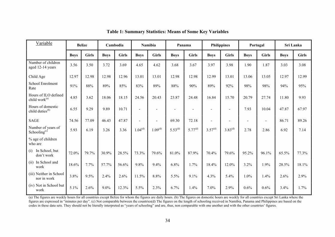
34

Table 1: Summary Statistics: Means of Some Key Variables

Belize Cambodia Namibia Panama Philippines Portugal Sri Lanka Variable

Boys Girls Boys Girls Boys Girls Boys Girls Boys Girls Boys Girls Boys Girls

Number of children aged 12-14 years 3.56 3.50 3.72 3.69 4.65 4.62 3.68 3.67 3.97 3.98 1.90 1.87 3.03 3.08

Child Age 12.97 12.98 12.98 12.96 13.01 13.01 12.98 12.98 12.99 13.01 13.06 13.05 12.97 12.99

School Enrolment Rate 91% 88% 89% 85% 83% 89% 88% 90% 89% 92% 98% 98% 94% 95%

Hours of ILO defined child work(a) 4.85 3.62 18.06 18.15 24.56 20.43 23.87 24.48 16.84 15.70 20.79 27.74 11.80 9.93

Hours of domestic child duties(b) 6.55 9.29 9.89 10.71 - - - - - - 7.93 10.04 47.87 67.97

SAGE 74.56 77.09 46.43 47.87 - - 69.30 72.18 - - - - 86.71 89.26

Number of years of Schooling(c) 5.93 6.19 3.26 3.36 1.04(d) 1.09(d) 5.53(d) 5.77(d) 3.57(d) 3.83(d) 2.78 2.86 6.92 7.14

% age of children who are

(i) In School, but don’t work 72.0% 79.7% 30.9% 28.5% 73.3% 79.6% 81.0% 87.9% 70.4% 79.6% 95.2% 96.1% 65.5% 77.3%

(ii) In School and work 18.6% 7.7% 57.7% 56.6% 9.8% 9.4% 6.8% 1.7% 18.4% 12.0% 3.2% 1.9% 28.5% 18.1%

(iii) Neither in School nor in work 3.8% 9.5% 2.4% 2.6% 11.5% 8.8% 5.5% 9.1% 4.3% 5.4% 1.0% 1.4% 2.6% 2.9%

(iv) Not in School but work 5.1% 2.6% 9.0% 12.3% 5.5% 2.3% 6.7% 1.4% 7.0% 2.9% 0.6% 0.6% 3.4% 1.7%

(a) The figures are weekly hours for all countries except Belize for whom the figures are daily hours. (b) The figures on domestic hours are weekly for all countries except Sri Lanka where the figures are expressed in “minutes per day”. (c) Not comparable between the countries(d) The figures on the length of schooling received in Namibia, Panama and Philippines are based on the codes in these data sets. They should not be literally interpreted as “years of schooling” and are, thus, non comparable with one another and with the other countries’ figures.

35

Table 2: Multinomial Logit Coefficient Estimates(a): Belize(e), (f), (g)

Category(b)

Variable School and Work Neither in School Nor in Work

Work Only

Age of child 7.93(c) (3.86)

-2.13 (6.97)

-4.58 (11.42)

(Age of child)2 -0.30(c) (0.15)

0.14 (0.26)

0.25 (0.43)

No. of children in the household

0.09(c) (.04)

0.06 (0.06)

0.00 (0.08)

Gender of household head (1 = male, 2 = female)

-0.35 (.18)

-0.49 (0.30)

-0.46 (0.38)

Gender of child (0 = girl,1 = boy)

1.08(d) (0.16)

-0.86(d) (0.22)

0.78(d) (0.27)

Years of Schooling 0.06 (0.06)

-0.34(d) (0.07)

-0.28(d) (0.09)

Dummy for Lighting -1.30(e) (0.63)

0.32 (0.52)

-0.44 (0.81)

Dummy for Water -0.46(d) (0.17)

0.98(d) (0.21)

0.34 (0.28)

Dummy for TV -.95(d) (0.17)

-0.74(d) (0.24)

-0.85(d) (0.28)

Dummy for Radio -.39 (0.22)

-0.45 (0.28)

0.44 (0.45)

Dummy for Telephone -.39(c) (0.18)

-1.02(d) (0.30)

-2.60(d) (0.61)

(a) Figures in brackets are standard errors. (b) The “school only” category is the normalised category. (c) Statistically significant at 5% significance level. (d) Statistically significant at 1% significance level. (e) Number of observations = 1894. (f) Likelihood Ratio Test of Joint Significance: 2

33529.13=χ

(g) Pseudo R2 = 0.1790

36

Table 3: Regression Coefficient Estimates(a) of Current School Attendance: Belize(d)

Variable IV(e), (f) OLS(e), (g)

Age of child 1.667(c) (0.480)

1.445(c) (0.365)

(Age of child)2 -0.067(c) (0.018)

-0.059(c) (0.014)

Number of children in the household

-0.001 (0.005)

-0.010(b) (0.004)

Gender of household head (1 = male, 2 = female)

-0.006 (0.023)

0.042(c) (0.016)

Gender of child (0 = girl,1 = boy)

0.096(c) (0.020)

.049(c) (0.013)

Work hours -0.510(c) (0.098)

-0.049(c) (0.013)

(Work hours)2 0.055(c) (0.011)

0.002 (0.001)

Test for Ho: Difference in coefficients is not systematic 21χ = 38.88(c)

(a) Figures in brackets are standard errors. (b) Statistically significant at 5% significance level. (c) Statistically significant at 1% significance level. (d) Number of observations = 1894 (e) F-tests for Joint Significance: IV: F(7,1886) = 28.32(c), OLS: F(7,1886) = 44.26(c) (f) IV: Root MSE = 0.373 (g) OLS: R2 = 0.1411, 2R = 0.1379, Root MSE = 0.285

37

Table 4: Regression Coefficient Estimates(a) of Years of Schooling: Belize(d)

Variable IV(e), (f) OLS(e), (g)

Age of child 1.049 (2.698)

-0.506 (1.571)

(Age of child)2 -0.013 (0.104)

0.043 (0.060)

Number of children in the household

-0.029 (0.030)

-0.090(c) (0.017)

Gender of household head (1 = male, 2 = female)

-0.237 (0.129)

0.100 (0.068)

Gender of child (0 = girl,1 = boy)

0.151 (0.113)

-0.183(c) (0.057)

Work hours -3.326(c) (0.552)

-0.080 (0.053)

(Work hours)2 0.378(c) (0.063)

0.007 (0.006)

Test for Ho: Difference in coefficients is not systematic 21χ = 103.98(c)

(a) Figures in brackets are standard errors. (b) Statistically significant at 5% significance level. (c) Statistically significant at 1% significance level. (d) Number of observations = 1894 (e) F-tests for Joint Significance: IV: F(7,1886) = 22.93(c), OLS: F(7,1886) = 52.16(c) (f) IV: Root MSE = 2.0962 (g) OLS: R2 = 0.1622, 2R = 0.1591, Root MSE = 1.2261

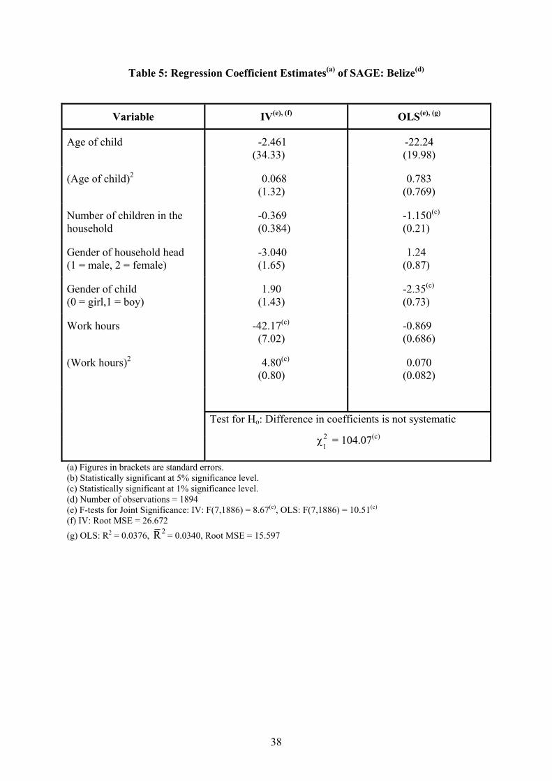
38

Table 5: Regression Coefficient Estimates(a) of SAGE: Belize(d)

Variable IV(e), (f) OLS(e), (g)

Age of child -2.461 (34.33)

-22.24 (19.98)

(Age of child)2 0.068 (1.32)

0.783 (0.769)

Number of children in the household

-0.369 (0.384)

-1.150(c) (0.21)

Gender of household head (1 = male, 2 = female)

-3.040 (1.65)

1.24 (0.87)

Gender of child (0 = girl,1 = boy)

1.90 (1.43)

-2.35(c) (0.73)

Work hours -42.17(c) (7.02)

-0.869 (0.686)

(Work hours)2 4.80(c) (0.80)

0.070 (0.082)

Test for Ho: Difference in coefficients is not systematic 21χ = 104.07(c)

(a) Figures in brackets are standard errors. (b) Statistically significant at 5% significance level. (c) Statistically significant at 1% significance level. (d) Number of observations = 1894 (e) F-tests for Joint Significance: IV: F(7,1886) = 8.67(c), OLS: F(7,1886) = 10.51(c) (f) IV: Root MSE = 26.672 (g) OLS: R2 = 0.0376, 2R = 0.0340, Root MSE = 15.597

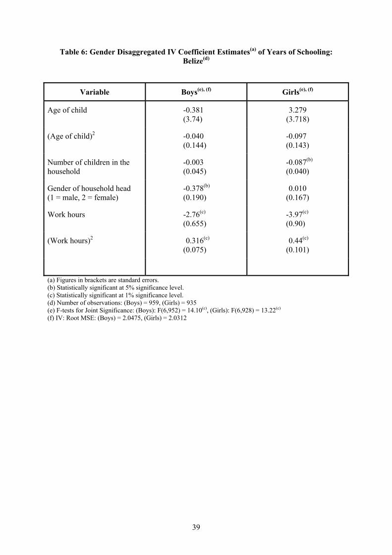
39

Table 6: Gender Disaggregated IV Coefficient Estimates(a) of Years of Schooling: Belize(d)

Variable Boys(e), (f) Girls(e), (f)

Age of child -0.381 (3.74)

3.279 (3.718)

(Age of child)2 -0.040 (0.144)

-0.097 (0.143)

Number of children in the household

-0.003 (0.045)

-0.087(b) (0.040)

Gender of household head (1 = male, 2 = female)

-0.378(b) (0.190)

0.010 (0.167)

Work hours -2.76(c) (0.655)

-3.97(c) (0.90)

(Work hours)2 0.316(c) (0.075)

0.44(c) (0.101)

(a) Figures in brackets are standard errors. (b) Statistically significant at 5% significance level. (c) Statistically significant at 1% significance level. (d) Number of observations: (Boys) = 959, (Girls) = 935 (e) F-tests for Joint Significance: (Boys): F(6,952) = 14.10(c), (Girls): F(6,928) = 13.22(c) (f) IV: Root MSE: (Boys) = 2.0475, (Girls) = 2.0312

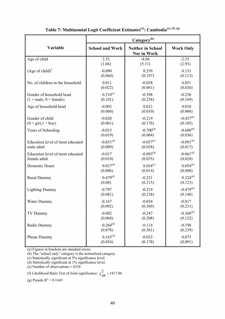
40

Table 7: Multinomial Logit Coefficient Estimates(a): Cambodia(e), (f), (g)

Category(b)

Variable School and Work Neither in School Nor in Work

Work Only

Age of child 2.53 (1.66)

-8.66 (5.11)

-2.35 (2.93)

(Age of child)2 -0.090 (0.064)

0.359 (0.197)

0.131 (0.113)

No. of children in the household 0.011 (0.022)

-0.038 (0.061)

0.051 (0.036)

Gender of household head (1 = male, 0 = female)

0.210(c) (0.101)

-0.398 (0.258)

-0.230 (0.169)

Age of household head -0.003 (0.004)

0.012 (0.010)

0.010 (0.006)

Gender of child (0 = girl,1 = boy)

-0.028 (0.061)

-0.219 (0.176)

-0.437(d) (0.105)

Years of Schooling -0.015 (0.019)

-0.700(d) (0.064)

-0.608(d) (0.036)

Education level of most educated male adult

-0.031(d) (0.009)

-0.057(c) (0.028)

-0.091(d) (0.017)

Education level of most educated female adult

-0.017 (0.010)

-0.093(d) (0.035)

-0.061(d) (0.020)

Domestic Hours 0.037(d) (0.006)

0.034(c) (0.014)

0.054(d) (0.008)

Rural Dummy 0.479(d) (0.08)

-0.221 (0.215)

0.324(d) (0.123)

Lighting Dummy -0.797 (0.081)

-0.219 (0.238)

-0.479(d) (0.148)

Water Dummy -0.167 (0.092)

-0.034 (0.369)

-0.017 (0.231)

TV Dummy -0.002 (0.068)

-0.247 (0.208)

-0.368(d) (0.122)

Radio Dummy -0.264(d) (0.078)

-0.114 (0.361)

-0.198 (0.239)

Phone Dummy 0.163(d) (0.054)

-0.032 (0.178)

0.073 (0.091)

(a) Figures in brackets are standard errors. (b) The “school only” category is the normalised category. (c) Statistically significant at 5% significance level. (d) Statistically significant at 1% significance level. (e) Number of observations = 6318

(f) Likelihood Ratio Test of Joint significance: 2 1817.8648χ =

(g) Pseudo R2 = 0.1443

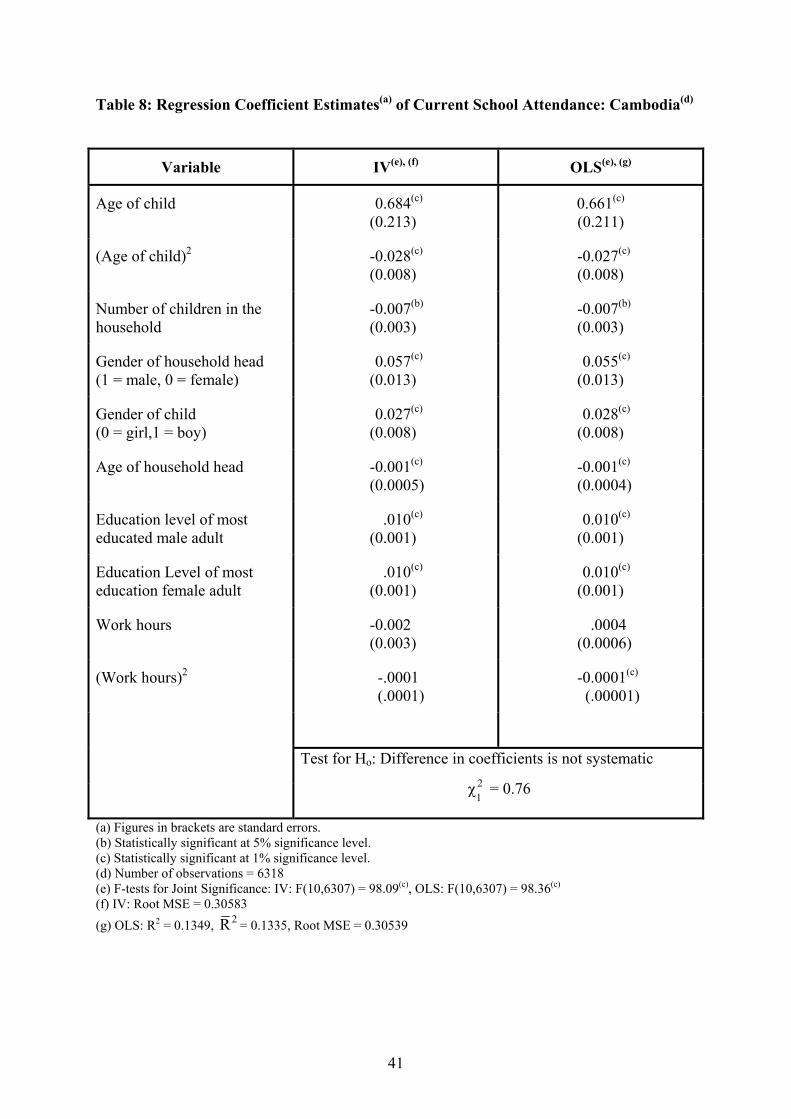
41

Table 8: Regression Coefficient Estimates(a) of Current School Attendance: Cambodia(d)

Variable IV(e), (f) OLS(e), (g)

Age of child 0.684(c) (0.213)

0.661(c) (0.211)

(Age of child)2 -0.028(c) (0.008)

-0.027(c) (0.008)

Number of children in the household

-0.007(b) (0.003)

-0.007(b) (0.003)

Gender of household head (1 = male, 0 = female)

0.057(c) (0.013)

0.055(c) (0.013)

Gender of child (0 = girl,1 = boy)

0.027(c) (0.008)

0.028(c) (0.008)

Age of household head -0.001(c) (0.0005)

-0.001(c) (0.0004)

Education level of most educated male adult

.010(c) (0.001)

0.010(c) (0.001)

Education Level of most education female adult

.010(c) (0.001)

0.010(c) (0.001)

Work hours -0.002 (0.003)

.0004 (0.0006)

(Work hours)2 -.0001 (.0001)

-0.0001(c) (.00001)

Test for Ho: Difference in coefficients is not systematic 21χ = 0.76

(a) Figures in brackets are standard errors. (b) Statistically significant at 5% significance level. (c) Statistically significant at 1% significance level. (d) Number of observations = 6318 (e) F-tests for Joint Significance: IV: F(10,6307) = 98.09(c), OLS: F(10,6307) = 98.36(c) (f) IV: Root MSE = 0.30583 (g) OLS: R2 = 0.1349, 2R = 0.1335, Root MSE = 0.30539

42

Table 9: Regression Coefficient Estimates(a) of Years of Schooling: Cambodia(d)

Variable IV(e), (f) OLS(e), (g)

Age of child 4.28(c) (1.67)

1.83 (1.15)

(Age of child)2 -0.135(b) (0.064)

-0.044 (0.044)

Number of children in the household

-0.107(c) (0.022)

-0.134(c) (0.015)

Gender of household head (1 = male, 0 = female)

0.363(c) (0.103)

0.203(c) (0.071)

Age of household head -0.010(c) (0.004)

-0.008(c) (0.002)

Gender of child (0 = girl,1 = boy)

-0.158(c) (0.060)

-0.114(c) (0.042)

Education level of most educated male adult

0.088(c) (0.010)

0.126(c) (0.006)

Education Level of most educated female adult

.021(c) (0.010)

0.148(c) (0.007)

Work hours -0.304(c) (0.025)

-0.014(c) (0.004)

(Work hours)2 0.005(c) (.0005)

-0.00007 (0.00007)

Test for Ho: Difference in coefficients is not systematic 21χ = 282.97(c)

(a) Figures in brackets are standard errors. (b) Statistically significant at 5% significance level. (c) Statistically significant at 1% significance level. (d) Number of observations = 6318 (e) F-tests for Joint Significance: IV: F(10,6307) = 158.78(c), OLS: F(10,6307) = 302.28(c) (f) IV: Root MSE = 2.3953 (g) OLS: R2 = 0.3240, 2R = 0.3229, Root MSE = 1.6601

43

Table 10: Regression Coefficient Estimates(a) of SAGE: Cambodia(d)

Variable IV(e), (f) OLS(e), (g)

Age of child 66.36(c) (24.04)

30.84 (16.42)

(Age of child)2 -2.40(c) (0.92)

-1.08 (0.63)

Number of children in the household

-1.51(c) (0.31)

-1.89(c) (0.22)

Gender of household head (1 = male, 0 = female)

5.14(c) (1.49)

2.82(c) (1.01)

Age of household head -0.13(c) (0.05)

-0.109(c) (0.035)

Gender of child (0 = girl,1 = boy)

-2.22(b) (0.87)

-1.58(c) (0.60)

Education level of most educated male adult

1.25(c) (0.14)

1.80(c) (0.09)

Education Level of most educated female adult

1.74(c) (0.14)

2.14(c) (0.10)

Work hours -4.40(c) (0.37)

-0.194(c) (0.050)

(Work hours)2 0.077(c) (0.007)

-0.0007 (0.001)

Test for Ho: Difference in coefficients is not systematic 21χ = 290.62(c)

(a) Figures in brackets are standard errors. (b) Statistically significant at 5% significance level. (c) Statistically significant at 1% significance level. (d) Number of observations = 6318 (e) F-tests for Joint Significance: IV: F(10,6307) = 126.00(c), OLS: F(10,6307) = 236.95(c) (f) IV: Root MSE = 34.452 (g) OLS: R2 = 0.2731, 2R = 0.2719, Root MSE = 23.711

44

Table 11: Regression Coefficient Estimates(a) of the Child’s Ability to Read and Write: Cambodia(d)

Variable IV(e), (f) OLS(e), (g)

Age of child 0.460 (0.237)

0.367 (0.231)

(Age of child)2 -0.016 (0.009)

-0.013 (0.009)

Number of children in the household

-0.013(c) (0.003)

-0.014(c) (0.003)

Gender of household head (1=male, 0=female)

0.064(c) (0.015)

0.058(c) (0.014)

Age of household head -0.0005 (0.0005)

-0.0004 (0.0004)

Gender of child (0=girl,1=boy)

-0.013 (0.009)

-0.011 (0.008)

Education level of most educated male adult

0.010(c) (0.001)

0.011(c) (0.001)

Education Level of most educated female adult

0.015(c) (0.001)

0.016(c) (0.001)

Work hours -0.012(c) (0.004)

-0.0015(b) (0.0007)

(Work hours)2 .0002(c) (.0001)

-0.00003 (0.00001)

Test for Ho: Difference in coefficients is not systematic 21χ = 10.00(c)

(a) Figures in brackets are standard errors. (b) Statistically significant at 5% significance level. (c) Statistically significant at 1% significance level. (d) Number of observations = 6318 (e) F-tests for Joint Significance: IV: F(10,6307) = 65.45(c), OLS: F(10,6307) = 67.15(c) (f) IV: Root MSE = 0.34011 (g) OLS: R2 = 0.0962, 2R = 0.0948, Root MSE = 0.33379

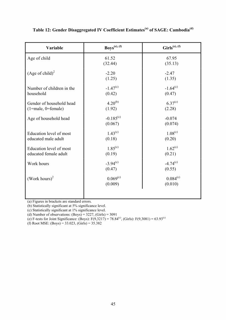
45

Table 12: Gender Disaggregated IV Coefficient Estimates(a) of SAGE: Cambodia(d)

Variable Boys(e), (f) Girls(e), (f)

Age of child 61.52 (32.44)

67.95 (35.13)

(Age of child)2 -2.20 (1.25)

-2.47 (1.35)

Number of children in the household

-1.47(c) (0.42)

-1.64(c) (0.47)

Gender of household head (1=male, 0=female)

4.20(b) (1.92)

6.37(c) (2.28)

Age of household head -0.185(c) (0.067)

-0.074 (0.074)

Education level of most educated male adult

1.43(c) (0.18)

1.08(c) (0.20)

Education level of most educated female adult

1.85(c) (0.19)

1.62(c) (0.21)

Work hours -3.94(c) (0.47)

-4.74(c) (0.55)

(Work hours)2 0.069(c) (0.009)

0.084(c) (0.010)

(a) Figures in brackets are standard errors. (b) Statistically significant at 5% significance level. (c) Statistically significant at 1% significance level. (d) Number of observations: (Boys) = 3227, (Girls) = 3091 (e) F-tests for Joint Significance: (Boys): F(9,3217) = 78.84(c), (Girls): F(9,3081) = 63.93(c) (f) Root MSE: (Boys) = 33.023, (Girls) = 35.382

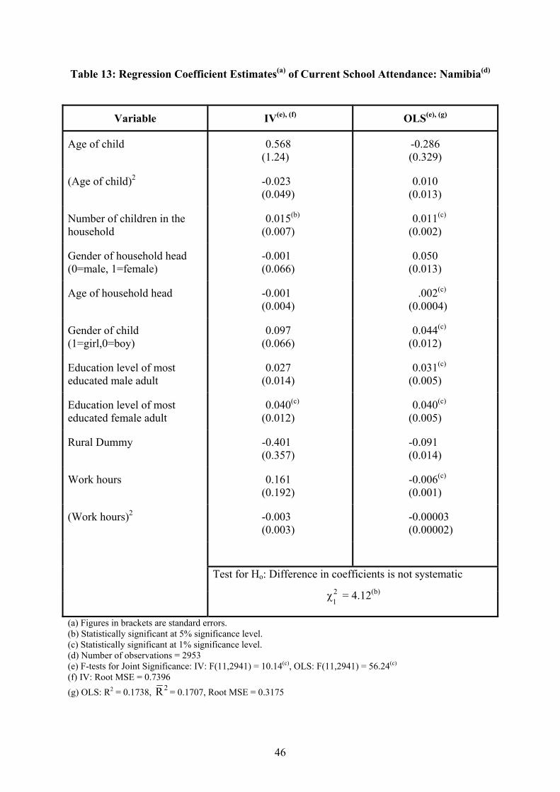
46

Table 13: Regression Coefficient Estimates(a) of Current School Attendance: Namibia(d)

Variable IV(e), (f) OLS(e), (g)

Age of child 0.568 (1.24)

-0.286 (0.329)

(Age of child)2 -0.023 (0.049)

0.010 (0.013)

Number of children in the household

0.015(b) (0.007)

0.011(c) (0.002)

Gender of household head (0=male, 1=female)

-0.001 (0.066)

0.050 (0.013)

Age of household head -0.001 (0.004)

.002(c) (0.0004)

Gender of child (1=girl,0=boy)

0.097 (0.066)

0.044(c) (0.012)

Education level of most educated male adult

0.027 (0.014)

0.031(c) (0.005)

Education level of most educated female adult

0.040(c) (0.012)

0.040(c) (0.005)

Rural Dummy -0.401 (0.357)

-0.091 (0.014)

Work hours 0.161 (0.192)

-0.006(c) (0.001)

(Work hours)2 -0.003 (0.003)

-0.00003 (0.00002)

Test for Ho: Difference in coefficients is not systematic 21χ = 4.12(b)

(a) Figures in brackets are standard errors. (b) Statistically significant at 5% significance level. (c) Statistically significant at 1% significance level. (d) Number of observations = 2953 (e) F-tests for Joint Significance: IV: F(11,2941) = 10.14(c), OLS: F(11,2941) = 56.24(c) (f) IV: Root MSE = 0.7396 (g) OLS: R2 = 0.1738, 2R = 0.1707, Root MSE = 0.3175

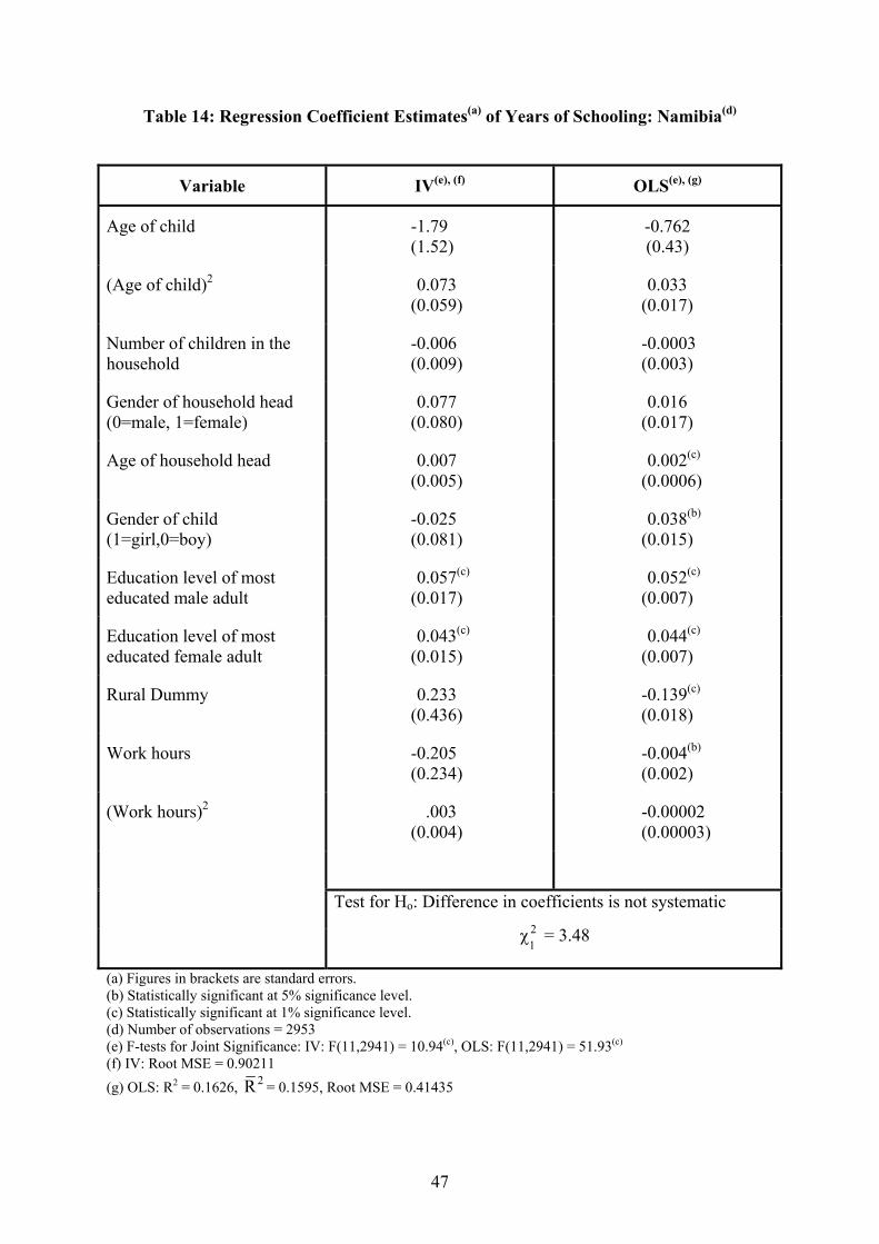
47

Table 14: Regression Coefficient Estimates(a) of Years of Schooling: Namibia(d)

Variable IV(e), (f) OLS(e), (g)

Age of child -1.79 (1.52)

-0.762 (0.43)

(Age of child)2 0.073 (0.059)

0.033 (0.017)

Number of children in the household

-0.006 (0.009)

-0.0003 (0.003)

Gender of household head (0=male, 1=female)

0.077 (0.080)

0.016 (0.017)

Age of household head 0.007 (0.005)

0.002(c) (0.0006)

Gender of child (1=girl,0=boy)

-0.025 (0.081)

0.038(b) (0.015)

Education level of most educated male adult

0.057(c) (0.017)

0.052(c) (0.007)

Education level of most educated female adult

0.043(c) (0.015)

0.044(c) (0.007)

Rural Dummy 0.233 (0.436)

-0.139(c) (0.018)

Work hours -0.205 (0.234)

-0.004(b) (0.002)

(Work hours)2 .003 (0.004)

-0.00002 (0.00003)

Test for Ho: Difference in coefficients is not systematic 21χ = 3.48

(a) Figures in brackets are standard errors. (b) Statistically significant at 5% significance level. (c) Statistically significant at 1% significance level. (d) Number of observations = 2953 (e) F-tests for Joint Significance: IV: F(11,2941) = 10.94(c), OLS: F(11,2941) = 51.93(c) (f) IV: Root MSE = 0.90211 (g) OLS: R2 = 0.1626, 2R = 0.1595, Root MSE = 0.41435

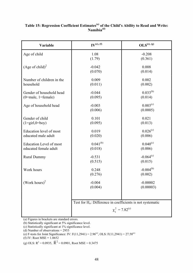
48

Table 15: Regression Coefficient Estimates(a) of the Child’s Ability to Read and Write: Namibia(d)

Variable IV(e), (f) OLS(e), (g)

Age of child 1.08 (1.79)

-0.208 (0.361)

(Age of child)2 -0.042 (0.070)

0.008 (0.014)

Number of children in the household

0.009 (0.011)

0.002 (0.002)

Gender of household head (0=male, 1=female)

-0.044 (0.095)

0.033(b) (0.014)

Age of household head -0.003 (0.006)

0.003(c) (0.0005)

Gender of child (1=girl,0=boy)

0.101 (0.095)

0.021 (0.013)

Education level of most educated male adult

0.019 (0.020)

0.026(c) (0.006)

Education Level of most educated female adult

0.041(b) (0.018)

0.040(c) (0.006)

Rural Dummy -0.531 (0.515)

-0.064(c) (0.015)

Work hours 0.248 (0.276)

-0.004(b) (0.002)

(Work hours)2 -0.004 (0.004)

-0.00002 (0.00003)

Test for Ho: Difference in coefficients is not systematic 21χ = 7.82(c)

(a) Figures in brackets are standard errors. (b) Statistically significant at 5% significance level. (c) Statistically significant at 1% significance level. (d) Number of observations = 2953 (e) F-tests for Joint Significance: IV: F(11,2941) = 2.96(c), OLS: F(11,2941) = 27.58(c) (f) IV: Root MSE = 1.0652 (g) OLS: R2 = 0.0935, 2R = 0.0901, Root MSE = 0.3475

49

Table 16: Gender Disaggregated IV Coefficient Estimates(a) of Years of Schooling: Namibia(d)

Variable Boys(e), (f) Girls(e), (f)

Age of child -0.441 (1.061)

-1.609(b) (0.772)

(Age of child)2 0.021 (0.041)

0.066(b) (0.030)

Number of children in the household

0.001 (0.007)

-0.005 (0.005)

Gender of household head (0=male, 1=female)

0.028 (0.043)

0.012 (0.046)

Age of household head 0.006(b) (0.003)

0.003(c) (0.001)

Education level of most educated male adult

0.048(c) (0.018)

0.060(c) (0.011)

Education Level of most educated female adult

0.051(c) (0.018)

0.041(c) (0.011)

Rural Dummy 0.113 (0.161)

-0.058 (0.102)

Work hours -0.152 (0.081)

-0.033 (0.056)

(Work hours)2 0.002 (0.001)

0.0004 (0.0008)

(a) Figures in brackets are standard errors. (b) Statistically significant at 5% significance level. (c) Statistically significant at 1% significance level. (d) Number of observations: (Boys) = 1465, (Girls) = 1488 (e) F-tests for Joint Significance: (Boys): F(10,1454) = 9.25(c), (Girls): F(10,1477) = 27.64(c) (f) Root MSE: (Boys) = 0.72315, (Girls) = 0.43129

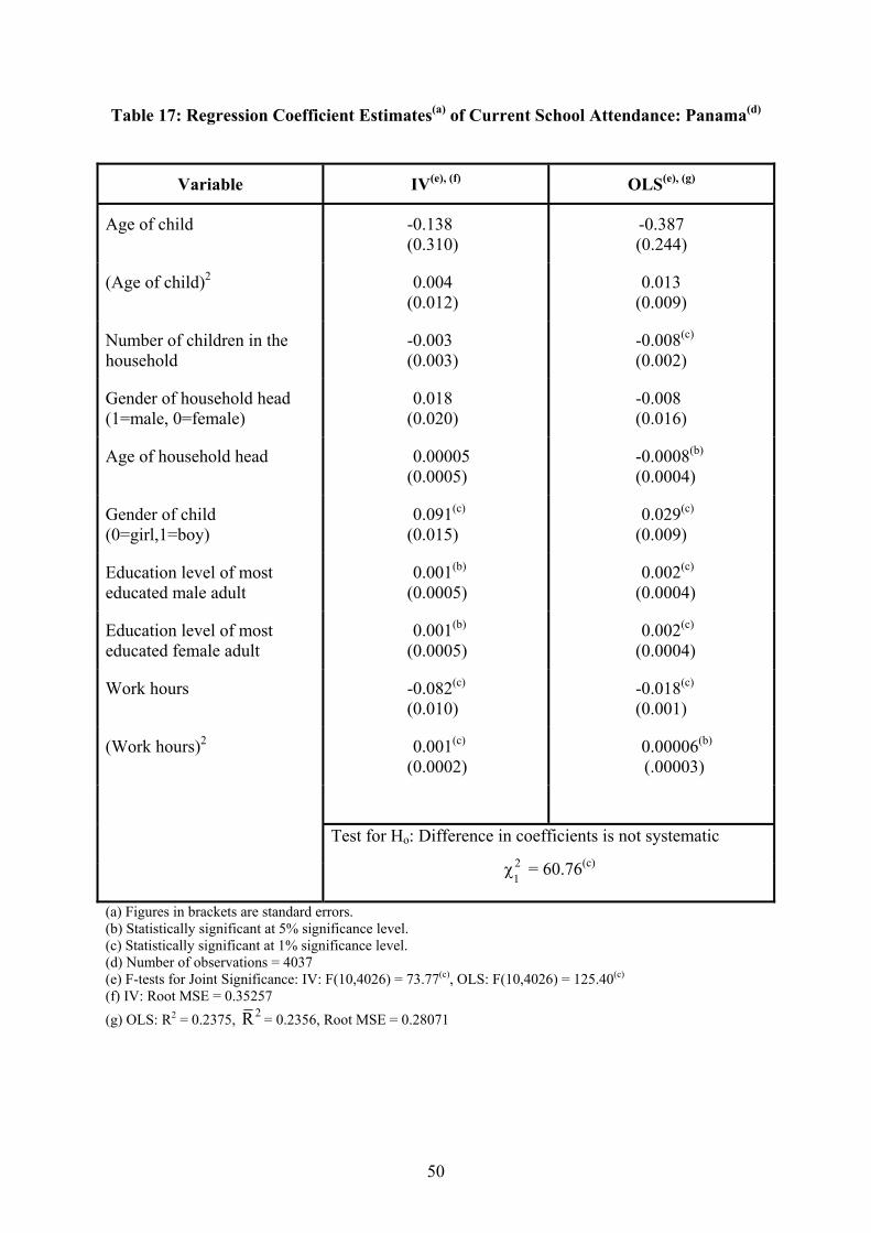
50

Table 17: Regression Coefficient Estimates(a) of Current School Attendance: Panama(d)

Variable IV(e), (f) OLS(e), (g)

Age of child -0.138 (0.310)

-0.387 (0.244)

(Age of child)2 0.004 (0.012)

0.013 (0.009)

Number of children in the household

-0.003 (0.003)

-0.008(c) (0.002)

Gender of household head (1=male, 0=female)

0.018 (0.020)

-0.008 (0.016)

Age of household head 0.00005 (0.0005)

-0.0008(b) (0.0004)

Gender of child (0=girl,1=boy)

0.091(c) (0.015)

0.029(c) (0.009)

Education level of most educated male adult

0.001(b) (0.0005)

0.002(c) (0.0004)

Education level of most educated female adult

0.001(b) (0.0005)

0.002(c) (0.0004)

Work hours -0.082(c) (0.010)

-0.018(c) (0.001)

(Work hours)2 0.001(c) (0.0002)

0.00006(b) (.00003)

Test for Ho: Difference in coefficients is not systematic 21χ = 60.76(c)

(a) Figures in brackets are standard errors. (b) Statistically significant at 5% significance level. (c) Statistically significant at 1% significance level. (d) Number of observations = 4037 (e) F-tests for Joint Significance: IV: F(10,4026) = 73.77(c), OLS: F(10,4026) = 125.40(c) (f) IV: Root MSE = 0.35257 (g) OLS: R2 = 0.2375, 2R = 0.2356, Root MSE = 0.28071

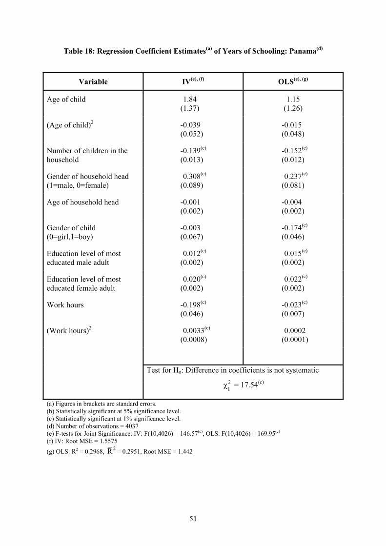
51

Table 18: Regression Coefficient Estimates(a) of Years of Schooling: Panama(d)

Variable IV(e), (f) OLS(e), (g)

Age of child 1.84 (1.37)

1.15 (1.26)

(Age of child)2 -0.039 (0.052)

-0.015 (0.048)

Number of children in the household

-0.139(c) (0.013)

-0.152(c) (0.012)

Gender of household head (1=male, 0=female)

0.308(c) (0.089)

0.237(c) (0.081)

Age of household head -0.001 (0.002)

-0.004 (0.002)

Gender of child (0=girl,1=boy)

-0.003 (0.067)

-0.174(c) (0.046)

Education level of most educated male adult

0.012(c) (0.002)

0.015(c) (0.002)

Education level of most educated female adult

0.020(c) (0.002)

0.022(c) (0.002)

Work hours -0.198(c) (0.046)

-0.023(c) (0.007)

(Work hours)2 0.0033(c) (0.0008)

0.0002 (0.0001)

Test for Ho: Difference in coefficients is not systematic 21χ = 17.54(c)

(a) Figures in brackets are standard errors. (b) Statistically significant at 5% significance level. (c) Statistically significant at 1% significance level. (d) Number of observations = 4037 (e) F-tests for Joint Significance: IV: F(10,4026) = 146.57(c), OLS: F(10,4026) = 169.95(c) (f) IV: Root MSE = 1.5575 (g) OLS: R2 = 0.2968, 2R = 0.2951, Root MSE = 1.442

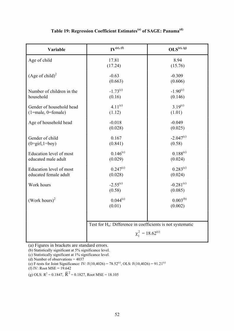
52

Table 19: Regression Coefficient Estimates(a) of SAGE: Panama(d)

Variable IV(e), (f) OLS(e), (g)

Age of child 17.81 (17.24)

8.94 (15.76)

(Age of child)2 -0.63 (0.663)

-0.309 (0.606)

Number of children in the household

-1.73(c) (0.16)

-1.90(c) (0.146)

Gender of household head (1=male, 0=female)

4.11(c) (1.12)

3.19(c) (1.01)

Age of household head -0.018 (0.028)

-0.049 (0.025)

Gender of child (0=girl,1=boy)

0.167 (0.841)

-2.047(c) (0.58)

Education level of most educated male adult

0.146(c) (0.029)

0.188(c) (0.024)

Education level of most educated female adult

0.247(c) (0.028)

0.283(c) (0.024)

Work hours -2.55(c) (0.58)

-0.281(c) (0.085)

(Work hours)2 0.044(c) (0.01)

0.003(b) (0.002)

Test for Ho: Difference in coefficients is not systematic 21χ = 18.62(c)

(a) Figures in brackets are standard errors. (b) Statistically significant at 5% significance level. (c) Statistically significant at 1% significance level. (d) Number of observations = 4037 (e) F-tests for Joint Significance: IV: F(10,4026) = 78.52(c), OLS: F(10,4026) = 91.21(c) (f) IV: Root MSE = 19.642 (g) OLS: R2 = 0.1847, 2R = 0.1827, Root MSE = 18.105

53

Table 20: Gender Disaggregated IV Coefficient Estimates(a) of SAGE: Panama(d)

Variable Boys(e), (f) Girls(e), (f)

Age of child -2.29 (23.41)

32.88 (22.91)

(Age of child)2 0.109 (0.90)

-1.19 (0.88)

Number of children in the household

-1.61(c) (0.22)

-1.99(c) (0.21)

Gender of household head (1=male, 0=female)

5.21(c) (1.54)

1.98 (1.46)

Age of household head 0.034 (0.038)

-0.109(c) (0.037)

Education level of most educated male adult

0.152(c) (0.040)

0.176(c) (0.035)

Education level of most educated female adult

0.285(c) (0.037)

0.237(c) (0.035)

Work hours -1.42(c) (0.48)

-3.53(b) (1.71)

(Work hours)2 0.023(c) (0.008)

0.07 (0.037)

(a) Figures in brackets are standard errors. (b) Statistically significant at 5% significance level. (c) Statistically significant at 1% significance level. (d) Number of observations: (Boys) = 2098, (Girls) = 1939 (e) F-tests for Joint Significance: (Boys): F(9,2088) = 49.86(c), (Girls): F(9,1929) = 45.25(c) (f) IV: Root MSE (Boys) = 19.14, (Girls) = 18.197

54

Table 21: Regression Coefficient Estimates(a) of Current School Attendance: Philippines(d)

Variable IV(e), (f) OLS(e), (g)

Age of child -2.17 (1.82)

0.196 (0.478)

(Age of child)2 0.085 (0.071)

-0.009 (0.018)

Seasonal Dummy (1=if the child work is seasonal, 0=otherwise)

-0.183 (0.143)

0.115(c) (0.019)

Years of Work 0.014 (0.016)

0.016(c) (0.005)

Gender of child (1=boy, 2=girl)

-0.068 (0.085)

0.081(c) (0.017)

Rural Dummy -0.004 (0.059)

-0.061(c) (0.017)

Work hours -0.220(b) (0.088)

-0.020(c) (0.0016)

(Work hours)2 0.003(b) (0.0013)

0.0001(c) (0.00003)

Test for Ho: Difference in coefficients is not systematic 21χ = 50.16(c)

(a) Figures in brackets are standard errors. (b) Statistically significant at 5% significance level. (c) Statistically significant at 1% significance level. (d) Number of observations = 1710 (e) F-tests for Joint Significance: IV: F(8,1701) = 10.86(c), OLS: F(8,1701) = 117.01(c) (f) IV: Root MSE = 1.0738 (g) OLS: R2 = 0.3550, 2R = 0.3519, Root MSE = 0.34466

55

Table 22: Regression Coefficient Estimates(a) of Years of Schooling: Philippines

Variable IV OLS

Age of child -7.08 (9.40)

5.51(c) (1.70)

(Age of child)2 0.314 (0.365)

-0.186(c) (0.065)

Seasonal Dummy (1=if the child work is seasonal, 0=otherwise)

-1.31 (0.74)

0.27(c) (0.066)

Years of Work -0.020 (0.082)

-0.007 (0.018)

Gender of child (1=boy, 2=girl)

-0.332 (0.441)

0.462(c) (0.062)

Rural Dummy -0.016 (0.304)

-0.321(c) (0.061)

Work hours -1.10(b) (0.46)

-0.033(c) (0.006)

(Work hours)2 0.016(b) (0.007)

0.0003(c) (0.0001)

Test for Ho: Difference in coefficients is not systematic 21χ = 112.34(c)

(a) Figures in brackets are standard errors.

(b) Statistically significant at 5% significance level. (c) Statistically significant at 1% significance level. (d) Number of observations = 1710 (e) F-tests for Joint Significance: IV: F(8,1701) = 3.50(c), OLS: F(8,1701) = 60.78(c) (f) IV: Root MSE = 5.5527 (g) OLS: R2 = 0.2223, 2R = 0.2186, Root MSE = 1.2264

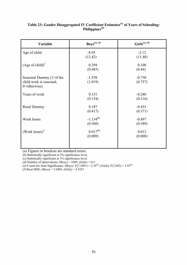
56

Table 23: Gender Disaggregated IV Coefficient Estimates(a) of Years of Schooling: Philippines(d)

Variable Boys(e), (f) Girls(e), (f)

Age of child -8.95 (12.42)

-2.12 (11.48)

(Age of child)2 0.394 (0.485)

0.108 (0.44)

Seasonal Dummy (1=if the child work is seasonal, 0=otherwise)

-1.558 (1.019)

-0.730 (0.757)

Years of work 0.151 (0.134)

-0.280 (0.216)

Rural Dummy 0.187 (0.417)

-0.433 (0.371)

Work hours -1.134(b) (0.560)

-0.897 (0.589)

(Work hours)2 0.017(b) (0.009)

0.012 (0.008)

(a) Figures in brackets are standard errors. (b) Statistically significant at 5% significance level. (c) Statistically significant at 1% significance level. (d) Number of observations: (Boys) = 1099, (Girls) = 611 (e) F-tests for Joint Significance: (Boys): F(7,1091) = 2.18(b), (Girls): F(7,603) = 1.92(b) (f) Root MSE: (Boys) = 5.6903, (Girls) = 4.5251

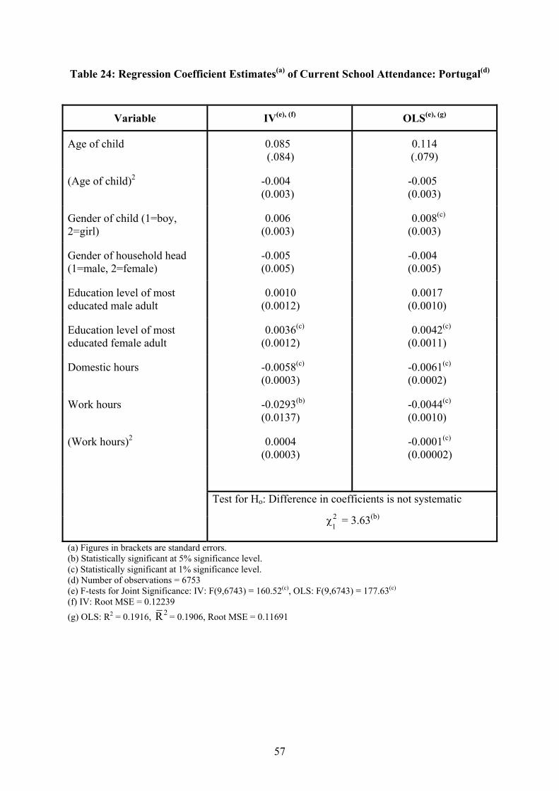
57

Table 24: Regression Coefficient Estimates(a) of Current School Attendance: Portugal(d)

Variable IV(e), (f) OLS(e), (g)

Age of child 0.085 (.084)

0.114 (.079)

(Age of child)2 -0.004 (0.003)

-0.005 (0.003)

Gender of child (1=boy, 2=girl)

0.006 (0.003)

0.008(c) (0.003)

Gender of household head (1=male, 2=female)

-0.005 (0.005)

-0.004 (0.005)

Education level of most educated male adult

0.0010 (0.0012)

0.0017 (0.0010)

Education level of most educated female adult

0.0036(c) (0.0012)

0.0042(c) (0.0011)

Domestic hours -0.0058(c) (0.0003)

-0.0061(c) (0.0002)

Work hours -0.0293(b) (0.0137)

-0.0044(c) (0.0010)

(Work hours)2 0.0004 (0.0003)

-0.0001(c) (0.00002)

Test for Ho: Difference in coefficients is not systematic 21χ = 3.63(b)

(a) Figures in brackets are standard errors. (b) Statistically significant at 5% significance level. (c) Statistically significant at 1% significance level. (d) Number of observations = 6753 (e) F-tests for Joint Significance: IV: F(9,6743) = 160.52(c), OLS: F(9,6743) = 177.63(c) (f) IV: Root MSE = 0.12239 (g) OLS: R2 = 0.1916, 2R = 0.1906, Root MSE = 0.11691

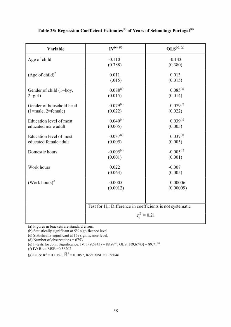
58

Table 25: Regression Coefficient Estimates(a) of Years of Schooling: Portugal(d)

Variable IV(e), (f) OLS(e), (g)

Age of child -0.110 (0.388)

-0.143 (0.380)

(Age of child)2 0.011 (.015)

0.013 (0.015)

Gender of child (1=boy, 2=girl)

0.088(c) (0.015)

0.085(c) (0.014)

Gender of household head (1=male, 2=female)

-0.079(c) (0.022)

-0.079(c) (0.022)

Education level of most educated male adult

0.040(c) (0.005)

0.039(c) (0.005)

Education level of most educated female adult

0.037(c) (0.005)

0.037(c) (0.005)

Domestic hours -0.005(c) (0.001)

-0.005(c) (0.001)

Work hours 0.022 (0.063)

-0.007 (0.005)

(Work hours)2 -0.0005 (0.0012)

0.00006 (0.00009)

Test for Ho: Difference in coefficients is not systematic 21χ = 0.21

(a) Figures in brackets are standard errors. (b) Statistically significant at 5% significance level. (c) Statistically significant at 1% significance level. (d) Number of observations = 6753 (e) F-tests for Joint Significance: IV: F(9,6743) = 88.98(c), OLS: F(9,6743) = 89.71(c) (f) IV: Root MSE =0.56202 (g) OLS: R2 = 0.1069, 2R = 0.1057, Root MSE = 0.56046

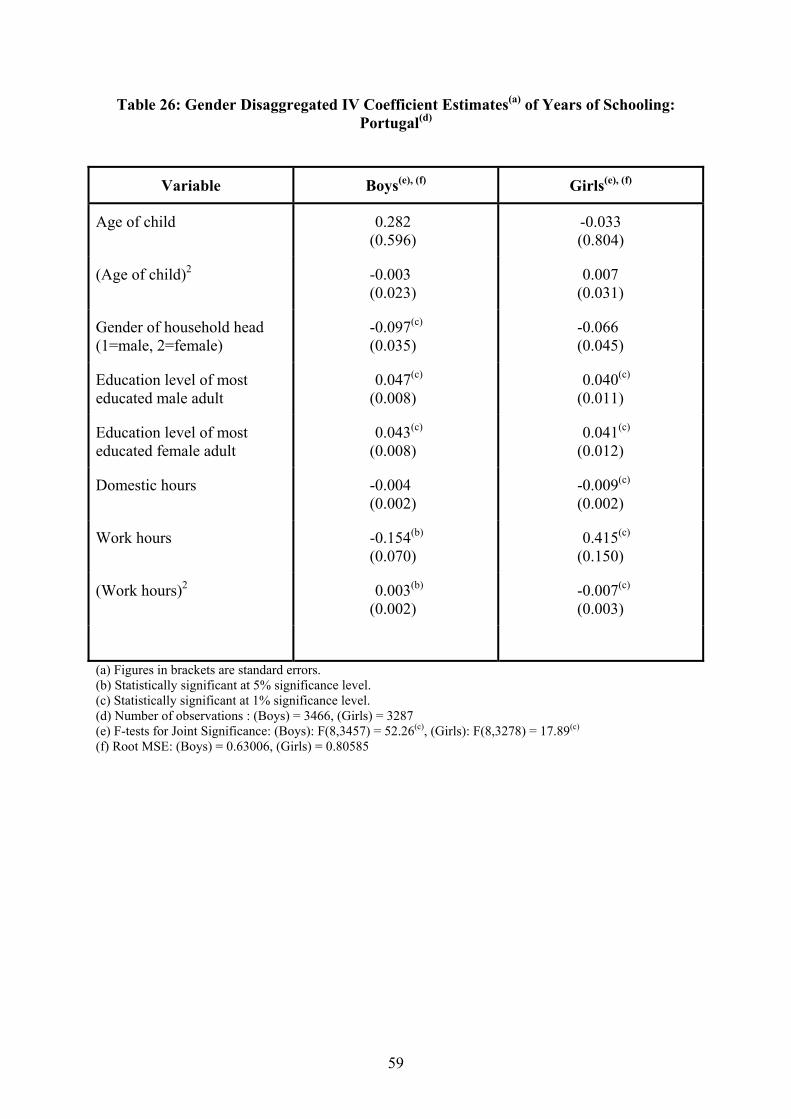
59

Table 26: Gender Disaggregated IV Coefficient Estimates(a) of Years of Schooling: Portugal(d)

Variable Boys(e), (f) Girls(e), (f)

Age of child 0.282 (0.596)

-0.033 (0.804)

(Age of child)2 -0.003 (0.023)

0.007 (0.031)

Gender of household head (1=male, 2=female)

-0.097(c) (0.035)

-0.066 (0.045)

Education level of most educated male adult

0.047(c) (0.008)

0.040(c) (0.011)

Education level of most educated female adult

0.043(c) (0.008)

0.041(c) (0.012)

Domestic hours -0.004 (0.002)

-0.009(c) (0.002)

Work hours -0.154(b) (0.070)

0.415(c) (0.150)

(Work hours)2 0.003(b) (0.002)

-0.007(c) (0.003)

(a) Figures in brackets are standard errors. (b) Statistically significant at 5% significance level. (c) Statistically significant at 1% significance level. (d) Number of observations : (Boys) = 3466, (Girls) = 3287 (e) F-tests for Joint Significance: (Boys): F(8,3457) = 52.26(c), (Girls): F(8,3278) = 17.89(c) (f) Root MSE: (Boys) = 0.63006, (Girls) = 0.80585

60

Table 27: Regression Coefficient Estimates(a) of Number of Failures Experienced

by the Child: Portugal(d)

Variable IV(e), (f) OLS(e), (g)

Age of child -0.049 (0.665)

-0.426 (0.569)

(Age of child)2 0.006 (0.026)

0.021 (0.022)

Gender of child (1=boy, 2=girl)

-0.211(c) (0.027)

-0.246(c) (0.021)

Gender of household head (1=male, 2=female)

0.098(c) (0.038)

0.095(c) (0.033)

Education level of most educated male adult

-0.083(c) (0.009)

-0.093(c) (0.008)

Education level of most educated female adult

-0.084(c) (0.009)

-0.092(c) (0.008)

Domestic hours 0.004(b) (0.002)

0.008(c) (0.002)

Work hours 0.334(c) (0.108)

0.009 (0.007)

(Work hours)2 -0.006(c) (0.002)

-0.0001 (0.0001)

Test for Ho: Difference in coefficients is not systematic 21χ = 11.98(c)

(a) Figures in brackets are standard errors. (b) Statistically significant at 5% significance level. (c) Statistically significant at 1% significance level. (d) Number of observations = 6753 (e) F-tests for Joint Significance: IV: F(9,6743) = 78.66(c), OLS: F(9,6743) = 102.38(c) (f) IV: Root MSE = 0.96397 (g) OLS: R2 = 0.1202, 2R = 0.1191, Root MSE = 0.83991

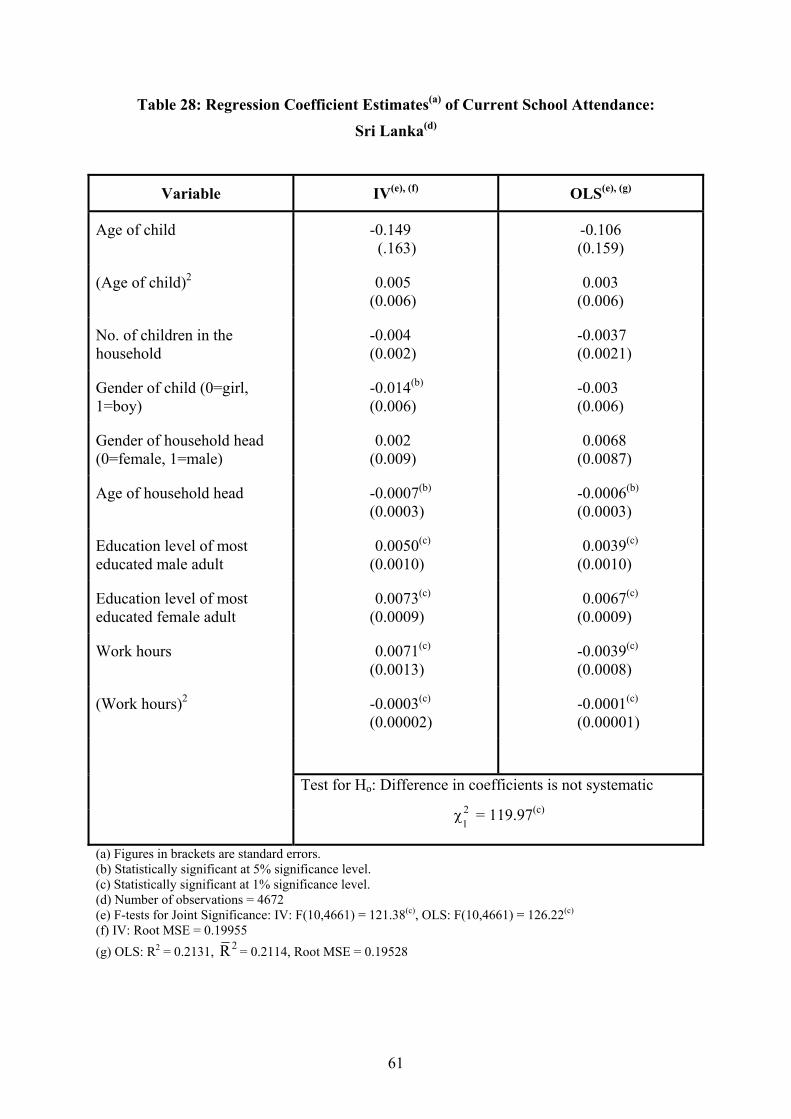
61

Table 28: Regression Coefficient Estimates(a) of Current School Attendance:

Sri Lanka(d)

Variable IV(e), (f) OLS(e), (g)

Age of child -0.149 (.163)

-0.106 (0.159)

(Age of child)2 0.005 (0.006)

0.003 (0.006)

No. of children in the household

-0.004 (0.002)

-0.0037 (0.0021)

Gender of child (0=girl, 1=boy)

-0.014(b) (0.006)

-0.003 (0.006)

Gender of household head (0=female, 1=male)

0.002 (0.009)

0.0068 (0.0087)

Age of household head -0.0007(b) (0.0003)

-0.0006(b) (0.0003)

Education level of most educated male adult

0.0050(c) (0.0010)

0.0039(c) (0.0010)

Education level of most educated female adult

0.0073(c) (0.0009)

0.0067(c) (0.0009)

Work hours 0.0071(c) (0.0013)

-0.0039(c) (0.0008)

(Work hours)2 -0.0003(c) (0.00002)

-0.0001(c) (0.00001)

Test for Ho: Difference in coefficients is not systematic 21χ = 119.97(c)

(a) Figures in brackets are standard errors. (b) Statistically significant at 5% significance level. (c) Statistically significant at 1% significance level. (d) Number of observations = 4672 (e) F-tests for Joint Significance: IV: F(10,4661) = 121.38(c), OLS: F(10,4661) = 126.22(c) (f) IV: Root MSE = 0.19955 (g) OLS: R2 = 0.2131, 2R = 0.2114, Root MSE = 0.19528

62

Table 29: Regression Coefficient Estimates(a) of Years of Schooling: Sri Lanka(d)

Variable IV(e), (f) OLS(e), (g)

Age of child 0.615 (1.103)

0.778 (1.096)

(Age of child)2 0.012 (0.042)

0.006 (0.042)

No. of children in the household

-0.057(c) (0.015)

-0.057(c) (0.015)

Study Time 0.002(c) (0.0002)

0.002(c) (0.0002)

Gender of child (0=girl, 1=boy)

-0.204(c) (0.041)

-0.166(c) (0.040)

Gender of household head (0=female, 1=male)

0.085 (0.061)

0.105 (0.060)

Age of household head -0.003 (0.002)

-0.003 (0.002)

Education level of most educated male adult

0.052(c) (0.007)

0.048(c) (0.007)

Education level of most educated female adult

0.073(c) (0.006)

0.071(c) (0.006)

Work hours 0.056(c) (0.009)

0.017(c) (0.005)

(Work hours)2 -0.0015(c) (0.0001)

-0.0010(c) (0.0001)

Test for Ho: Difference in coefficients is not systematic 21χ = 31.43(c)

(a) Figures in brackets are standard errors. (b) Statistically significant at 5% significance level. (c) Statistically significant at 1% significance level. (d) Number of observations = 4672 (e) F-tests for Joint Significance: IV: F(11,4660) = 230.51(c), OLS: F(11,4660) = 230.40(c) (f) IV: Root MSE = 1.3535 (g) OLS: R2 = 0.3523, 2R = 0.3507, Root MSE = 1.3457

63

Table 30: Regression Coefficient Estimates(a) of Study Time: Sri Lanka(d)

Variable IV(e), (f) OLS(e), (g)

Age of child 141.86 (75.89)

146.92 (75.76)

(Age of child)2 -5.28 (2.92)

-5.46 (2.91)

No. of children in the household

-0.154 (1.02)

-0.149 (1.021)

Gender of child (0=girl, 1=boy)

-16.02(c) (2.80)

-14.71(c) (2.75)

Gender of household head (0=female, 1=male)

10.10(b) (4.18)

10.72(b) (4.16)

Age of household head -0.176 (0.135)

-0.169 (0.135)

Education level of most educated male adult

1.76(c) (0.46)

1.63(c) (0.46)

Education level of most educated female adult

2.58(c) (0.41)

2.51(c) (0.41)

Work hours 0.117 (0.607)

-1.18(c) (0.37)

(Work hours)2 -0.024(c) (0.010)

-0.004 (0.007)

Test for Ho: Difference in coefficients is not systematic 21χ = 7.25(c)

(a) Figures in brackets are standard errors. (b) Statistically significant at 5% significance level. (c) Statistically significant at 1% significance level. (d) Number of observations = 4672 (e) F-tests for Joint Significance: IV: F(10,4661) = 22.50(c), OLS: F(10,4661) = 23.60(c) (f) IV: Root MSE = 93.163 (g) OLS: R2 = 0.0482, 2R = 0.0461, Root MSE = 93.038

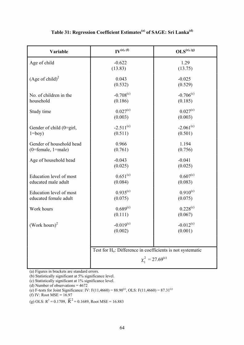
64

Table 31: Regression Coefficient Estimates(a) of SAGE: Sri Lanka(d)

Variable IV(e), (f) OLS(e), (g)

Age of child -0.622 (13.83)

1.29 (13.75)

(Age of child)2 0.043 (0.532)

-0.025 (0.529)

No. of children in the household

-0.708(c) (0.186)

-0.706(c) (0.185)

Study time 0.027(c) (0.003)

0.027(c) (0.003)

Gender of child (0=girl, 1=boy)

-2.511(c) (0.511)

-2.061(c) (0.501)

Gender of household head (0=female, 1=male)

0.966 (0.761)

1.194 (0.756)

Age of household head -0.043 (0.025)

-0.041 (0.025)

Education level of most educated male adult

0.651(c) (0.084)

0.607(c) (0.083)

Education level of most educated female adult

0.935(c) (0.075)

0.910(c) (0.075)

Work hours 0.689(c) (0.111)

0.228(c) (0.067)

(Work hours)2 -0.019(c) (0.002)

-0.012(c) (0.001)

Test for Ho: Difference in coefficients is not systematic 21χ = 27.69(c)

(a) Figures in brackets are standard errors. (b) Statistically significant at 5% significance level. (c) Statistically significant at 1% significance level. (d) Number of observations = 4672 (e) F-tests for Joint Significance: IV: F(11,4660) = 88.90(c), OLS: F(11,4660) = 87.31(c) (f) IV: Root MSE = 16.97 (g) OLS: R2 = 0.1709, 2R = 0.1689, Root MSE = 16.883

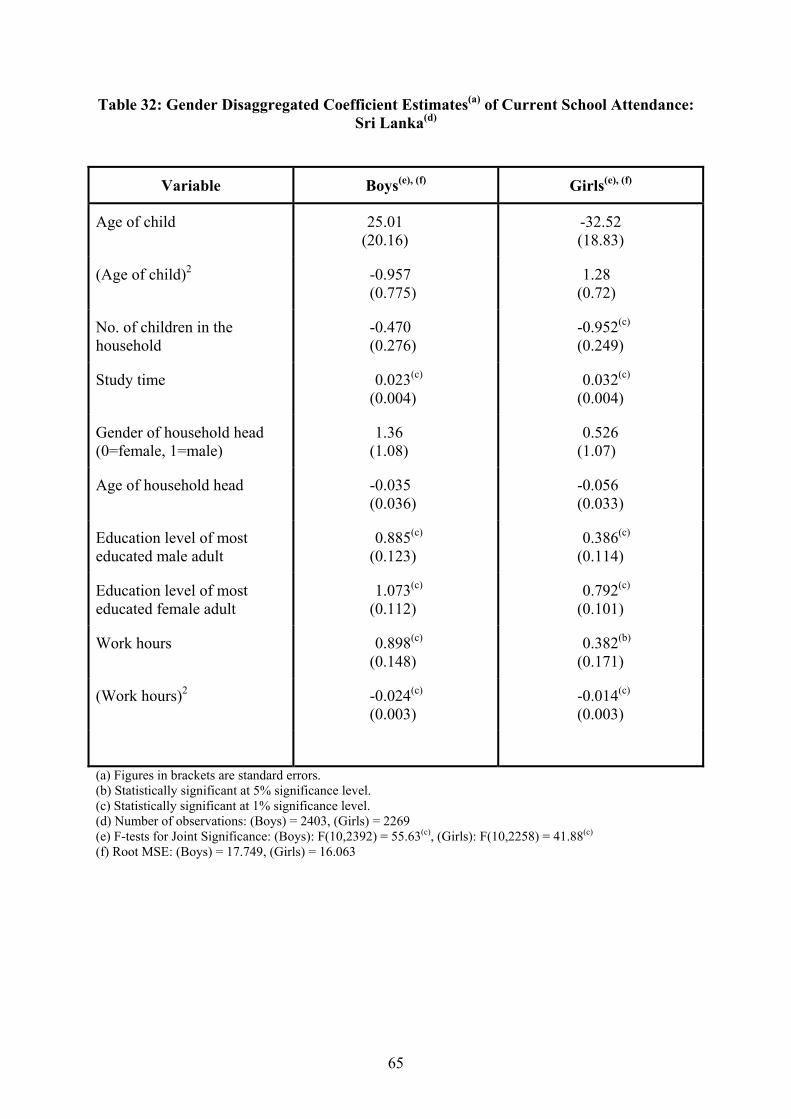
65

Table 32: Gender Disaggregated Coefficient Estimates(a) of Current School Attendance: Sri Lanka(d)

Variable Boys(e), (f) Girls(e), (f)

Age of child 25.01 (20.16)

-32.52 (18.83)

(Age of child)2 -0.957 (0.775)

1.28 (0.72)

No. of children in the household

-0.470 (0.276)

-0.952(c) (0.249)

Study time 0.023(c) (0.004)

0.032(c) (0.004)

Gender of household head (0=female, 1=male)

1.36 (1.08)

0.526 (1.07)

Age of household head -0.035 (0.036)

-0.056 (0.033)

Education level of most educated male adult

0.885(c) (0.123)

0.386(c) (0.114)

Education level of most educated female adult

1.073(c) (0.112)

0.792(c) (0.101)

Work hours 0.898(c) (0.148)

0.382(b) (0.171)

(Work hours)2 -0.024(c) (0.003)

-0.014(c) (0.003)

(a) Figures in brackets are standard errors. (b) Statistically significant at 5% significance level. (c) Statistically significant at 1% significance level. (d) Number of observations: (Boys) = 2403, (Girls) = 2269 (e) F-tests for Joint Significance: (Boys): F(10,2392) = 55.63(c), (Girls): F(10,2258) = 41.88(c) (f) Root MSE: (Boys) = 17.749, (Girls) = 16.063

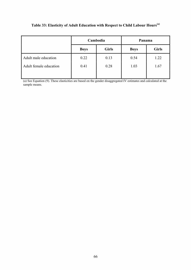
66

Table 33: Elasticity of Adult Education with Respect to Child Labour Hours(a)

Cambodia Panama

Boys Girls Boys Girls

Adult male education 0.22 0.13 0.54 1.22

Adult female education 0.41 0.28 1.03 1.67

(a) See Equation (9). These elasticities are based on the gender disaggregated IV estimates and calculated at the sample means.

67

Table 34: 3 SLS Coefficient Estimates(a) of SAGE on Selected SIMPOC Data Sets

Variable Belize Cambodia Panama Sri Lanka

Age of child -10.68 (35.33)

46.39 (26.65)

18.40 (17.64)

-2.03 (13.62)

(Age of child)2 0.411 (1.358)

-1.58 (1.02)

-0.64 (0.678)

0.098 (.524)

No. of children in the household

-0.285 (0.396)

-1.18(c) (0.35)

-1.70(c) (.17)

-0.572(c) (.184)

Gender of child (0=girl, 1=boy)

2.70 (1.51)

-1.94(b) (0.96)

0.554 (.878)

-1.712(c) (.525)

Age of household head - -.106 (0.056)

-.035 (.029)

-0.029 (.024)

Education level of most educated male adult

- 1.12(c) (.15)

.149(c) (.03)

.532(c) (.083)

Education level of most educated female adult

- 1.53(c) (.16)

.240(c) (.029)

.818(c)

(0.74)

Work hours -33.43 (7.37)

-3.76(c) (.55)

-2.18(c) (.63)

0.370(c) (.091)

(Work hours)2 3.37 (0.84)

.044(c) (.010)

.028(c) (.011)

-0.014(c) (.002)

Domestic hours -.009 (.082)

.416(c) (.127)

- -.017(c) (.006)

Rural Dummy - 0.88 (1.31)

2.34(c) (.78)

-

Phone Dummy - - 1.86(b) (.85)

-

Number of observations 1894 6318 4037 4638 (a) Figures in brackets are standard errors. (b) Statistically significant at 5% significance level. (c) Statistically significant at 1% significance level.

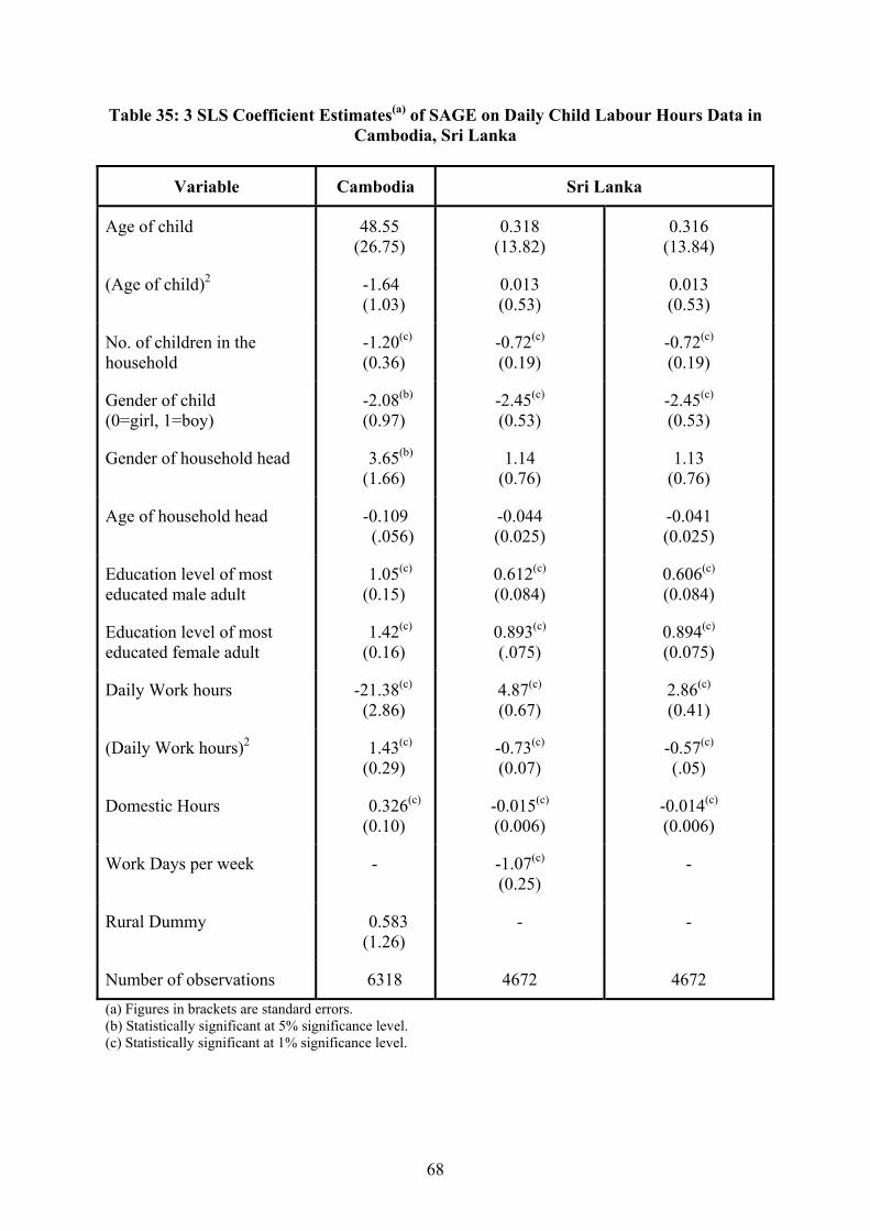
68

Table 35: 3 SLS Coefficient Estimates(a) of SAGE on Daily Child Labour Hours Data in Cambodia, Sri Lanka

Variable Cambodia Sri Lanka

Age of child 48.55 (26.75)

0.318 (13.82)

0.316 (13.84)

(Age of child)2 -1.64 (1.03)

0.013 (0.53)

0.013 (0.53)

No. of children in the household

-1.20(c) (0.36)

-0.72(c) (0.19)

-0.72(c) (0.19)

Gender of child (0=girl, 1=boy)

-2.08(b) (0.97)

-2.45(c) (0.53)

-2.45(c) (0.53)

Gender of household head 3.65(b) (1.66)

1.14 (0.76)

1.13 (0.76)

Age of household head -0.109 (.056)

-0.044 (0.025)

-0.041 (0.025)

Education level of most educated male adult

1.05(c) (0.15)

0.612(c) (0.084)

0.606(c) (0.084)

Education level of most educated female adult

1.42(c) (0.16)

0.893(c) (.075)

0.894(c) (0.075)

Daily Work hours -21.38(c) (2.86)

4.87(c) (0.67)

2.86(c) (0.41)

(Daily Work hours)2 1.43(c) (0.29)

-0.73(c) (0.07)

-0.57(c) (.05)

Domestic Hours 0.326(c)

(0.10) -0.015(c) (0.006)

-0.014(c) (0.006)

Work Days per week - -1.07(c) (0.25)

-

Rural Dummy 0.583 (1.26)

- -

Number of observations 6318 4672 4672 (a) Figures in brackets are standard errors. (b) Statistically significant at 5% significance level. (c) Statistically significant at 1% significance level.

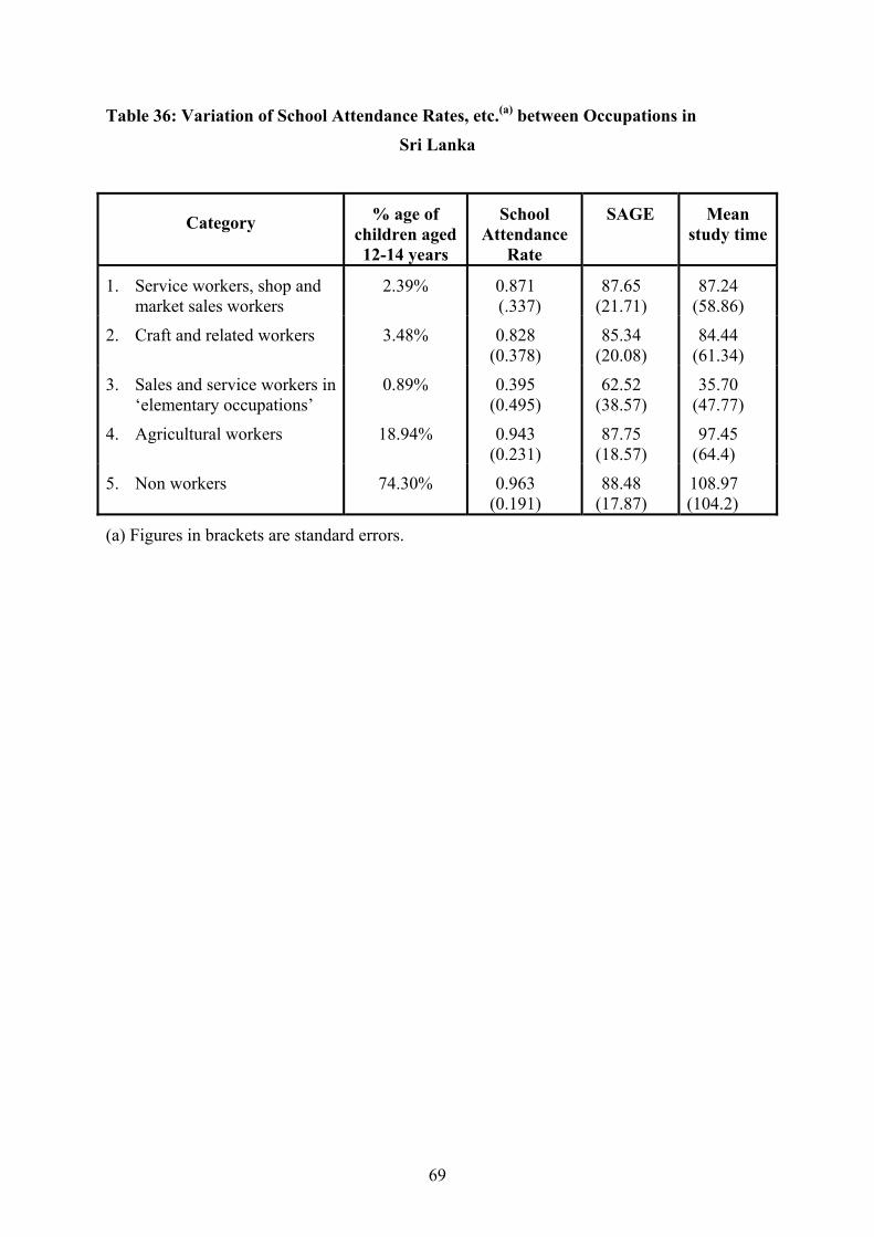
69

Table 36: Variation of School Attendance Rates, etc.(a) between Occupations in

Sri Lanka

Category % age of children aged 12-14 years

School Attendance

Rate

SAGE Mean study time

1. Service workers, shop and market sales workers

2.39% 0.871 (.337)

87.65 (21.71)

87.24 (58.86)

2. Craft and related workers 3.48% 0.828 (0.378)

85.34 (20.08)

84.44 (61.34)

3. Sales and service workers in ‘elementary occupations’

0.89% 0.395 (0.495)

62.52 (38.57)

35.70 (47.77)

4. Agricultural workers 18.94% 0.943 (0.231)

87.75 (18.57)

97.45 (64.4)

5. Non workers 74.30% 0.963 (0.191)

88.48 (17.87)

108.97 (104.2)

(a) Figures in brackets are standard errors.

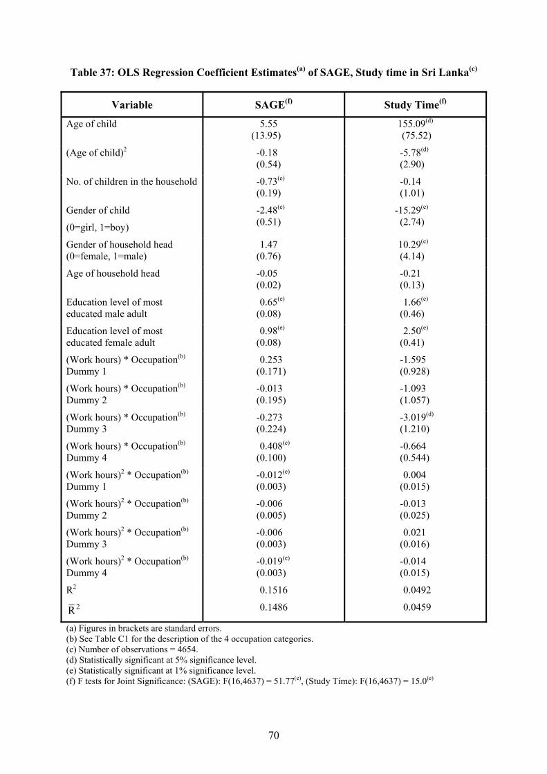
70

Table 37: OLS Regression Coefficient Estimates(a) of SAGE, Study time in Sri Lanka(c)

Variable SAGE(f) Study Time(f)

Age of child 5.55 (13.95)

155.09(d)

(75.52)

(Age of child)2 -0.18 (0.54)

-5.78(d)

(2.90)

No. of children in the household -0.73(e)

(0.19) -0.14 (1.01)

Gender of child

(0=girl, 1=boy)

-2.48(e)

(0.51) -15.29(e)

(2.74)

Gender of household head (0=female, 1=male)

1.47 (0.76)

10.29(e)

(4.14)

Age of household head -0.05 (0.02)

-0.21 (0.13)

Education level of most educated male adult

0.65(e)

(0.08) 1.66(e)

(0.46)

Education level of most educated female adult

0.98(e)

(0.08) 2.50(e)

(0.41)

(Work hours) * Occupation(b) Dummy 1

0.253 (0.171)

-1.595 (0.928)

(Work hours) * Occupation(b) Dummy 2

-0.013 (0.195)

-1.093 (1.057)

(Work hours) * Occupation(b) Dummy 3

-0.273 (0.224)

-3.019(d)

(1.210)

(Work hours) * Occupation(b) Dummy 4

0.408(e)

(0.100) -0.664 (0.544)

(Work hours)2 * Occupation(b) Dummy 1

-0.012(e)

(0.003) 0.004

(0.015)

(Work hours)2 * Occupation(b) Dummy 2

-0.006 (0.005)

-0.013 (0.025)

(Work hours)2 * Occupation(b) Dummy 3

-0.006 (0.003)

0.021 (0.016)

(Work hours)2 * Occupation(b) Dummy 4

-0.019(e)

(0.003) -0.014 (0.015)

R2 0.1516 0.0492 2R 0.1486 0.0459

(a) Figures in brackets are standard errors. (b) See Table C1 for the description of the 4 occupation categories. (c) Number of observations = 4654. (d) Statistically significant at 5% significance level. (e) Statistically significant at 1% significance level. (f) F tests for Joint Significance: (SAGE): F(16,4637) = 51.77(e), (Study Time): F(16,4637) = 15.0(e)

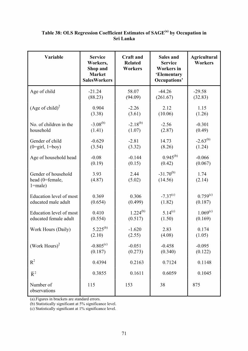
71

Table 38: OLS Regression Coefficient Estimates of SAGE(a) by Occupation in Sri Lanka

Variable Service Workers, Shop and Market

SalesWorkers

Craft and Related Workers

Sales and Service

Workers in ‘Elementary Occupations’

Agricultural Workers

Age of child -21.24 (88.23)

58.07 (94.09)

-44.26 (261.67)

-29.58 (32.83)

(Age of child)2 0.904 (3.38)

-2.26 (3.61)

2.12 (10.06)

1.15 (1.26)

No. of children in the household

-3.08(b) (1.41)

-2.18(b) (1.07)

-2.56 (2.87)

-0.301 (0.49)

Gender of child (0=girl, 1=boy)

-0.629 (3.54)

-2.81 (3.32)

14.73 (8.26)

-2.63(b) (1.24)

Age of household head -0.08 (0.19)

-0.144 (0.15)

0.945(b) (0.42)

-0.066 (0.067)

Gender of household head (0=female, 1=male)

3.93 (4.87)

2.44 (5.02)

-31.70(b) (14.56)

1.74 (2.14)

Education level of most educated male adult

0.369 (0.654)

0.306 (0.499)

-7.37(c) (1.82)

0.759(c) (0.187)

Education level of most educated female adult

0.410 (0.554)

1.224(b) (0.517)

5.14(c) (1.50)

1.069(c) (0.169)

Work Hours (Daily) 5.225(b) (2.10)

-1.620 (2.55)

2.83 (4.08)

0.174 (1.05)

(Work Hours)2 -0.805(c) (0.187)

-0.051 (0.273)

-0.458 (0.340)

-0.095 (0.122)

R2 0.4394 0.2163 0.7124 0.1148

2R 0.3855 0.1611 0.6059 0.1045

Number of observations

115 153 38 875

(a).Figures in brackets are standard errors. (b) Statistically significant at 5% significance level. (c) Statistically significant at 1% significance level.

72

References

Akabayashi, H. and G. Psacharopoulos (1999), “The trade-off between child labour and human capital formation: A Tanzanian case study”, Journal of Development Studies, 35(5), 120-140.

Basu, K. (1999), “Child Labour: Cause, Consequence and Cure with Remarks on International Labour Standards”, Journal of Economic Literature, 37, 1083-1119.

Basu, K. and Z. Tzannatos (2002), “The Global Child Labour Problem: What Do We Know and What Can We Do?”, mimeographed.

Bhalotra, S. (2000), “Is child work necessary?”, STICERD, LSE, Discussion Paper, NO. 26.

Bhalotra, S. and C. Heady, (2001), “Child Activities in South Asia and Sub-Saharan Africa” in P. Lawrence and C. Thirtle, eds., Africa and Asia in Comparative Development, London: Macmillan.

Bhalotra, S. and Z. Tzannatos, (2002), “Child Labour: What Have We Learnt?”, mimeographed.

Glewwe, P. (2002), “Schools and Skills in Developing Countries: Education Policies and Socioeconomic Outcomes”, Journal of Economic Literature, Vol. XL, 436-482.

Grootaert, C. and H.A. Patrinos, (1999), The Policy Analysis of Child Labour: A Comparative Study, (New York, St. Martin’s Press).

Heady, C. (2000), “What is the Effect of Child Labour on Learning Achievement? Evidence from Ghana”, Innocenti Working Paper NO. 79, Florence: UNICEF Innocenti Research Centre.

Hoddinott, J. and B. Kinsey (2001), “Child Growth in the Time of Drought”, Oxford Bulletin of Economics and Statistics, 63(4), 409-436.

Jensen, P. and H.S. Nielsen, (1997), “Child Labour on School Attendance: Evidence from Zambia”, Journal of Population Economics, 10, 407-424.

Kanbargi, R. and P.M. Kulkarni (1991), “Child work, schooling and fertility in rural Karnataka, India”, in R. Kanbargi (ed.), Child Labour in the Indian Subcontinent, Sage.

Maitra, P. and R. Ray (2002), “The Joint Estimation of Child Participation in Schooling and Employment: Comparative Evidence from Three Continents”, Oxford Development Studies, 30(1), 41-62.

Orazem, P. and V. Gunnarsson (2003), “Child Labour, School Attendance and Academic Performance: A Review”, mimeographed, March.

Patrinos, H.A. and G. Psacharopoulos (1995), “Educational performance and child labour in Paraguay”, International Journal of Educational Development, 15(1), 47-60.

Patrinos, H.A. and G. Psacharopoulos (1997), “Family size, schooling and child labour in Peru – an empirical analysis”, Journal of Population Economics, 10, 387-405.

Psacharopoulos, G. (1997), “Child Labour versus Educational Attainment: Some Evidence from Latin America”, Journal of Population Economics, 10, 337-386.

Ravallion, M. and Wodon, Q. (2000), “Does Child Labour displace Schooling? Evidence on behavioural responses to an enrolment subsidy”, The Economic Journal, 110 (462), C158-C175.

73

Ray, R. (2000a), “Analysis of child labour in Peru and Pakistan: a comparative study”, Journal of Population Economics, 13(1), 3-19.

Ray, R. (2000b), “Child labour, child schooling and their interaction with adult labour”, The World Bank Economic Review, 14, 347-367.

Ray, R. (2000c), “Poverty, Household Size and Child Welfare in India”, Economic and Political Weekly, 35, 3511-3520.

Ray, R. (2002), “The Determinants of Child Labour and Child Schooling in Ghana”, Journal of African Economies, 11(4), 561-590.

Rosati, F.C. and M. Rossi (2001), “Children’s Working Hours, School Enrolment and Human Capital Accumulation: Evidence from Pakistan and Nicaragua”, Understanding Children’s Work, UNICEF Innocenti Research Centre.

Rosati, F.C and Z. Tzannatos (2000), “Child Labour in Vietnam”, mimeo, The World Bank, Washington.

Sen, A.K. (1999), Development as Freedom, OUP, New York.

Singh, K. (1998), “Part-time Employment in High School and its Effect on Academic Achievement”, Journal of Educational Research, 91, 131-139.

Stewart, J. and L. Gill (1998), Econometrics, 2nd Edition, Prentice Hal, London.

Weiner, M. (1991), The Child and the State in India, Princeton: Princeton University Press.

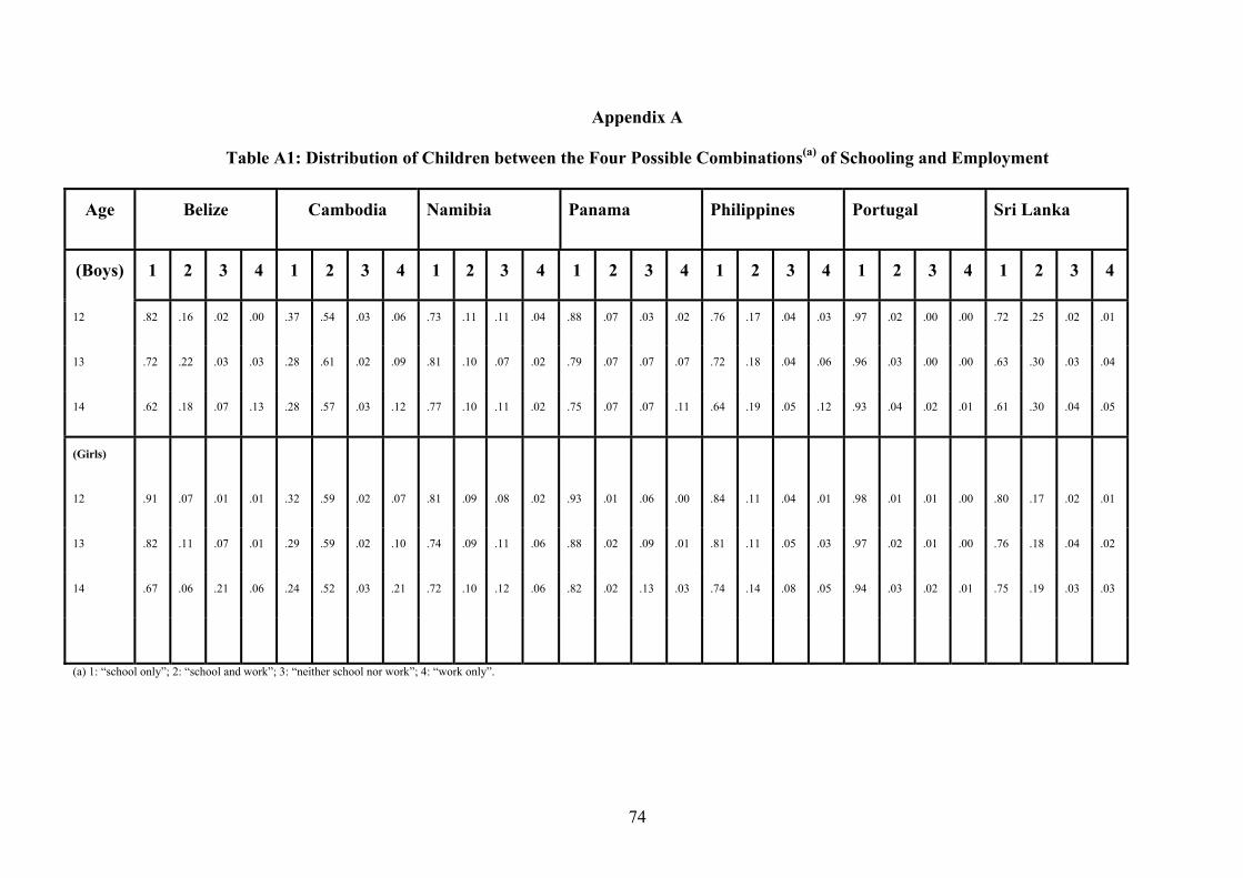
74

Appendix A

Table A1: Distribution of Children between the Four Possible Combinations(a) of Schooling and Employment

Age Belize Cambodia Namibia Panama Philippines Portugal Sri Lanka

(Boys) 1 2 3 4 1 2 3 4 1 2 3 4 1 2 3 4 1 2 3 4 1 2 3 4 1 2 3 4

12 .82 .16 .02 .00 .37 .54 .03 .06 .73 .11 .11 .04 .88 .07 .03 .02 .76 .17 .04 .03 .97 .02 .00 .00 .72 .25 .02 .01

13 .72 .22 .03 .03 .28 .61 .02 .09 .81 .10 .07 .02 .79 .07 .07 .07 .72 .18 .04 .06 .96 .03 .00 .00 .63 .30 .03 .04

14 .62 .18 .07 .13 .28 .57 .03 .12 .77 .10 .11 .02 .75 .07 .07 .11 .64 .19 .05 .12 .93 .04 .02 .01 .61 .30 .04 .05

(Girls)

12 .91 .07 .01 .01 .32 .59 .02 .07 .81 .09 .08 .02 .93 .01 .06 .00 .84 .11 .04 .01 .98 .01 .01 .00 .80 .17 .02 .01

13 .82 .11 .07 .01 .29 .59 .02 .10 .74 .09 .11 .06 .88 .02 .09 .01 .81 .11 .05 .03 .97 .02 .01 .00 .76 .18 .04 .02

14 .67 .06 .21 .06 .24 .52 .03 .21 .72 .10 .12 .06 .82 .02 .13 .03 .74 .14 .08 .05 .94 .03 .02 .01 .75 .19 .03 .03

(a) 1: “school only”; 2: “school and work”; 3: “neither school nor work”; 4: “work only”.

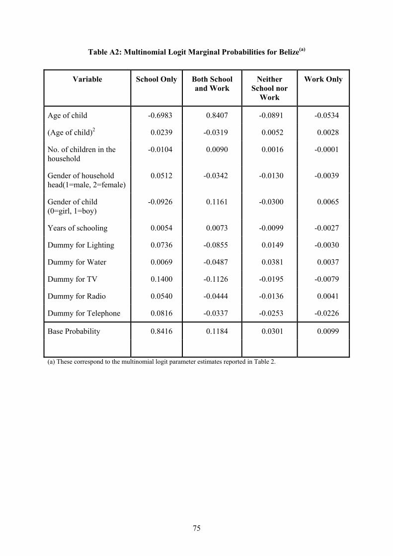
75

Table A2: Multinomial Logit Marginal Probabilities for Belize(a)

Variable School Only Both School and Work

Neither School nor

Work

Work Only

Age of child -0.6983 0.8407 -0.0891 -0.0534

(Age of child)2 0.0239 -0.0319 0.0052 0.0028

No. of children in the household

-0.0104 0.0090 0.0016 -0.0001

Gender of household head(1=male, 2=female)

0.0512 -0.0342 -0.0130 -0.0039

Gender of child (0=girl, 1=boy)

-0.0926 0.1161 -0.0300 0.0065

Years of schooling 0.0054 0.0073 -0.0099 -0.0027

Dummy for Lighting 0.0736 -0.0855 0.0149 -0.0030

Dummy for Water 0.0069 -0.0487 0.0381 0.0037

Dummy for TV 0.1400 -0.1126 -0.0195 -0.0079

Dummy for Radio 0.0540 -0.0444 -0.0136 0.0041

Dummy for Telephone 0.0816 -0.0337 -0.0253 -0.0226

Base Probability 0.8416 0.1184 0.0301 0.0099

(a) These correspond to the multinomial logit parameter estimates reported in Table 2.

76

Table A3: Multinomial Logit Marginal Probabilities for Cambodia

Variable School Only Both School and Work

Neither School nor

Work

Work Only

Age of child -0.4075 0.7301 -0.1288 -0.1938

(Age of child)2 0.0136 -0.0280 0.0052 0.0092

No. of children in the household

-0.0028 0.0012 -0.0006 0.0021

Gender of household head(1=male, 2=female)

-0.0334 0.0617 -0.0081 -0.0203

Age of household head 0.0004 -0.0012 0.0002 0.0006

Gender of child (0=girl, 1=boy)

0.0126 0.0102 -0.0023 -0.0206

Years of schooling 0.0146 0.0226 -0.0083 -0.0289

Education level of most educated male adult

0.0074 -0.0036 -0.0004 -0.0034

Education level of most educated female adult

0.0045 -0.0012 -0.0010 -0.0024

Domestic hours -0.0080 0.0065 0.00008 0.0014

Rural Dummy -0.0939 0.1008 -0.0070 0.00009

Lighting Dummy 0.1604 -0.1670 0.0040 0.0026

Water Dummy 0.0324 -0.0381 0.0010 0.0048

TV Dummy 0.0069 0.0137 -0.0029 -0.0178

Telephone Dummy 0.0529 -0.0529 0.0009 -0.0008

Radio Dummy -0.0315 0.0351 -0.0018 -0.0018

Base Probability 0.2910 0.6440 0.0130 0.0520

(a) These correspond to the multinomial logit parameter estimates reported in Table 7.

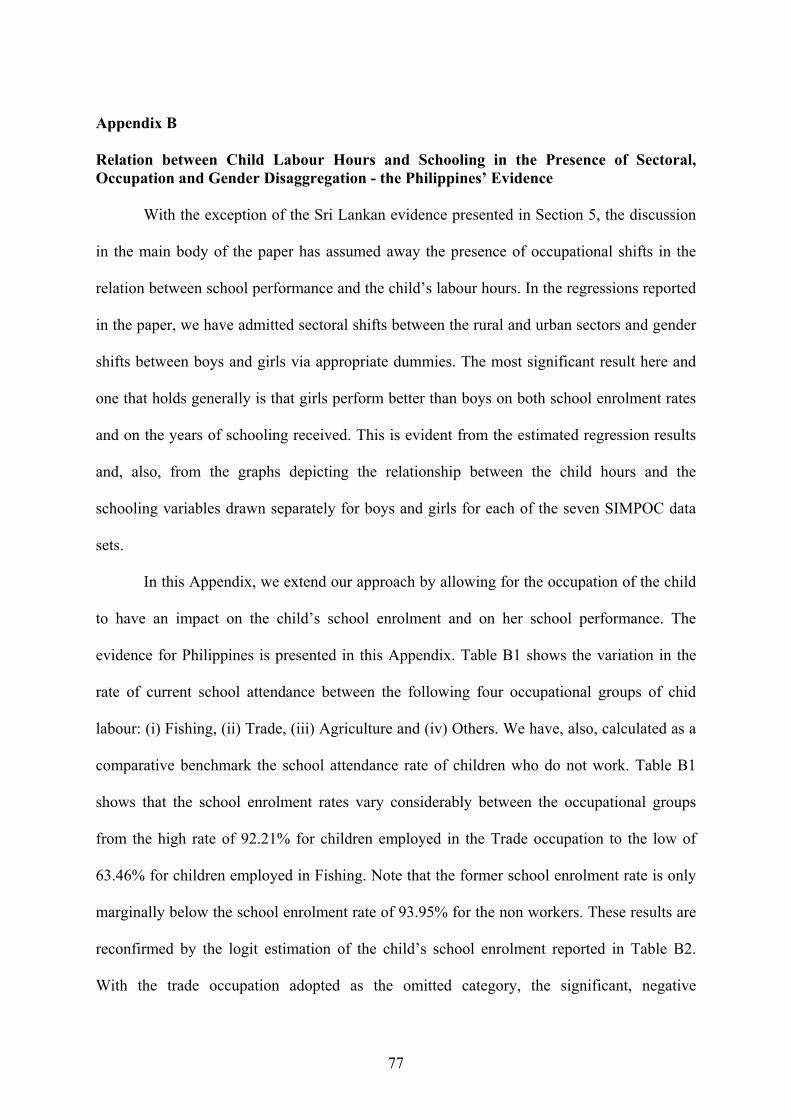
77

Appendix B Relation between Child Labour Hours and Schooling in the Presence of Sectoral, Occupation and Gender Disaggregation - the Philippines’ Evidence With the exception of the Sri Lankan evidence presented in Section 5, the discussion

in the main body of the paper has assumed away the presence of occupational shifts in the

relation between school performance and the child’s labour hours. In the regressions reported

in the paper, we have admitted sectoral shifts between the rural and urban sectors and gender

shifts between boys and girls via appropriate dummies. The most significant result here and

one that holds generally is that girls perform better than boys on both school enrolment rates

and on the years of schooling received. This is evident from the estimated regression results

and, also, from the graphs depicting the relationship between the child hours and the

schooling variables drawn separately for boys and girls for each of the seven SIMPOC data

sets.

In this Appendix, we extend our approach by allowing for the occupation of the child

to have an impact on the child’s school enrolment and on her school performance. The

evidence for Philippines is presented in this Appendix. Table B1 shows the variation in the

rate of current school attendance between the following four occupational groups of chid

labour: (i) Fishing, (ii) Trade, (iii) Agriculture and (iv) Others. We have, also, calculated as a

comparative benchmark the school attendance rate of children who do not work. Table B1

shows that the school enrolment rates vary considerably between the occupational groups

from the high rate of 92.21% for children employed in the Trade occupation to the low of

63.46% for children employed in Fishing. Note that the former school enrolment rate is only

marginally below the school enrolment rate of 93.95% for the non workers. These results are

reconfirmed by the logit estimation of the child’s school enrolment reported in Table B2.

With the trade occupation adopted as the omitted category, the significant, negative

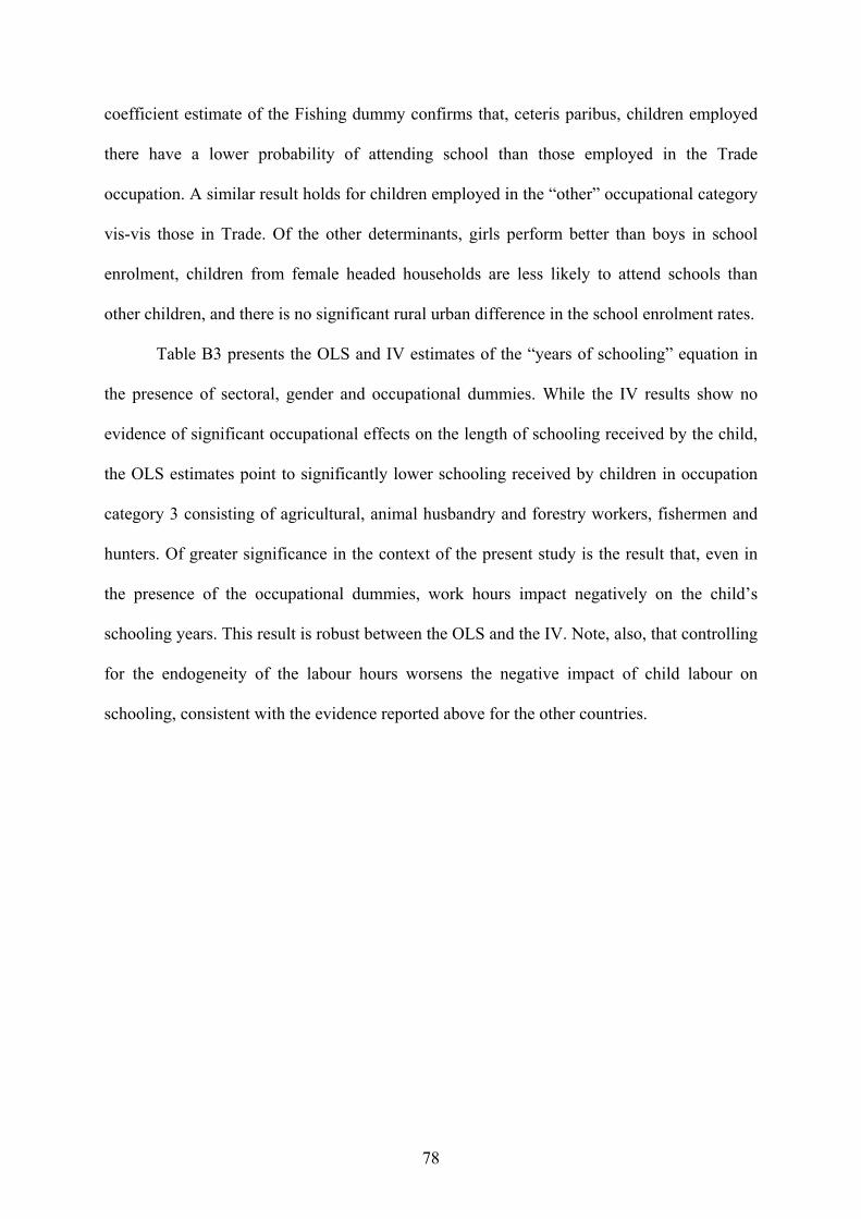
78

coefficient estimate of the Fishing dummy confirms that, ceteris paribus, children employed

there have a lower probability of attending school than those employed in the Trade

occupation. A similar result holds for children employed in the “other” occupational category

vis-vis those in Trade. Of the other determinants, girls perform better than boys in school

enrolment, children from female headed households are less likely to attend schools than

other children, and there is no significant rural urban difference in the school enrolment rates.

Table B3 presents the OLS and IV estimates of the “years of schooling” equation in

the presence of sectoral, gender and occupational dummies. While the IV results show no

evidence of significant occupational effects on the length of schooling received by the child,

the OLS estimates point to significantly lower schooling received by children in occupation

category 3 consisting of agricultural, animal husbandry and forestry workers, fishermen and

hunters. Of greater significance in the context of the present study is the result that, even in

the presence of the occupational dummies, work hours impact negatively on the child’s

schooling years. This result is robust between the OLS and the IV. Note, also, that controlling

for the endogeneity of the labour hours worsens the negative impact of child labour on

schooling, consistent with the evidence reported above for the other countries.

79

Table B1: Variation of School Attendance Rates between Occupations in the Philippines

Category School Attendance Rate(a)

Fishing 0.635 (0.484)

Trade 0.922 (0.268)

Agriculture 0.786 (0.410)

Others 0.785 (0.412)

Non Workers 0.940 (0.238)

(a) Figures in brackets indicate standard errors.

80

Table B2: Logit Coefficient Estimates(a) of School Enrolment in the Philippines

Variable Coefficient Estimate

Age of child 1.15 (4.18)

(Age of child)2 -0.08 (0.16)

No. of children in the household .008 (.040)

Gender of child (1=boy, 2=girl)

.396(b) (.162)

Gender of household head (1=male, 2=female)

-.728(b) (.307)

Education level of most educated male adult

.130(c) (.042)

Education level of most educated female adult

.092(b) (.044)

Years of Schooling .479(c) (0.062)

Rural Dummy .175 (.162)

Fishing Dummy -.836(b) (.359)

Agriculture Dummy -.354 (.283)

“Other” Dummy -.673 (.345)

(a) Standard Errors in brackets. (b) Statistical significance at 5% significance level. (c) Statistical significance at 1% significance level.

81

Table B3: Regression Coefficient Estimates(a) of Years of Schooling in the Philippines(i)

Variable IV(g), (i) OLS(h), (i)

Age of child -5.76 (8.61)

5.57(f) (1.67)

(Age of child)2 0.26 (0.33)

-0.19(f) (0.06)

Seasonal Dummy -1.19 (0.71)

.28(f) (.06)

Years of work -0.05 (0.08)

0.01 (0.02)

Gender of child

(1=boy, 2=girl)

-0.16 (0.34)

.32(f) (.06)

Rural Dummy -0.027 (.274)

-.113 (0.065)

Occupational Category No. 1 Dummy(b)

.215 (.52)

.139 (.13)

Occupational Category No. 2 Dummy(c)

-1.77 (1.02)

-.028 (.16)

Occupational Category No. 3 Dummy(d)

-.19 (.49)

-.483(f) (.11)

Work hours -.99(e) (.43)

-.03(f) (.006)

(Work hours)2 .015(e) (.006)

.0002(f) (.0001)

Test for Ho: Difference in coefficients is not systematic 21χ = 86.27(f)

(a) Figures in brackets are standard errors. (b) Occupational category 1 consists of clerical and related workers (c) Occupational category 2 consists of service workers (d) Occupational category 3 consists of agricultural, animal husbandry and forestry workers, fishermen and hunters. (e) Statistically significant at 5% significance level. (f) Statistically significant at 1% significance level. (g) IV: Root MSE = 5.0151 (h) OLS: R2 = 0.2502, 2R = 0.2453, Root MSE = 1.2053 (i) F tests for Joint Significance: IV: F(11,1698) = 3.30(f), OLS: F(11,1698) = 51.50(f) (j) Number of observations = 1710.

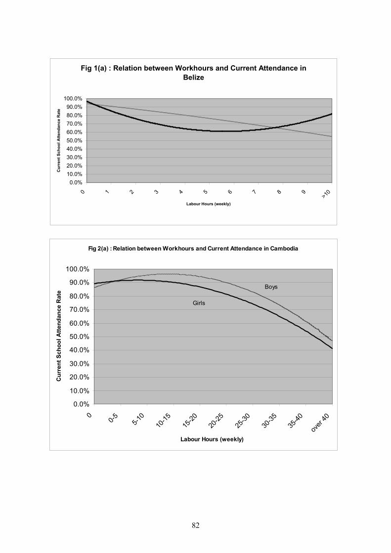
82

Fig 1(a) : Relation between Workhours and Current Attendance in Belize

0.0%10.0%20.0%30.0%40.0%50.0%60.0%70.0%80.0%90.0%

100.0%

0 1 2 3 4 5 6 7 8 9>1

0

Labour Hours (weekly)

Cur

rent

Sch

ool A

ttend

ance

Rat

e

Fig 2(a) : Relation between Workhours and Current Attendance in Cambodia

0.0%

10.0%

20.0%

30.0%

40.0%

50.0%

60.0%

70.0%

80.0%

90.0%

100.0%

00-5 5-1

010

-1515

-2020

-2525

-3030

-3535

-40

over

40

Labour Hours (weekly)

Cur

rent

Sch

ool A

ttend

ance

Rat

e

Girls

Boys

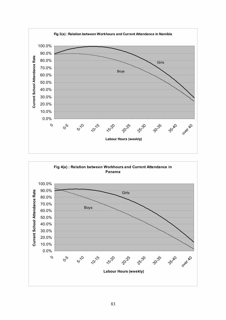
83

Fig 3(a) : Relation between Workhours and Current Attendance in Namibia

0.0%

10.0%

20.0%

30.0%

40.0%

50.0%

60.0%

70.0%

80.0%

90.0%

100.0%

00-5 5-1

010

-1515

-2020

-2525

-3030

-3535

-40

over

40

Labour Hours (weekly)

Cur

rent

Sch

ool A

ttend

ance

Rat

e

Girls

Boys

Fig 4(a) : Relation between Workhours and Current Attendance in Panama

0.0%10.0%

20.0%30.0%

40.0%50.0%

60.0%70.0%

80.0%90.0%

100.0%

00-5 5-1

010

-1515

-2020

-2525

-3030

-3535

-40

over

40

Labour Hours (weekly)

Cur

rent

Sch

ool A

ttend

ance

Rat

e Girls

Boys

84

Fig 5(a) : Relation between Workhours and Current Attendance in Philippines

0.0%

10.0%20.0%

30.0%

40.0%

50.0%60.0%

70.0%

80.0%90.0%

100.0%

00-5 5-1

010

-1515

-2020

-2525

-3030

-3535

-40

over

40

Labour Hours (weekly)

Cur

rent

Sch

ool A

ttend

ance

Rat

e

Girls

Boys

Fig 6(a) : Relation between Workhours and Current Attendance in Portugal

0.0%

10.0%

20.0%

30.0%

40.0%

50.0%

60.0%

70.0%

80.0%

90.0%

100.0%

00-5 5-1

010

-1515

-2020

-2525

-3030

-3535

-40

over

40

Labour Hours (weekly)

Cur

rent

Sch

ool A

ttend

ance

Rat

e

Girls

Boys

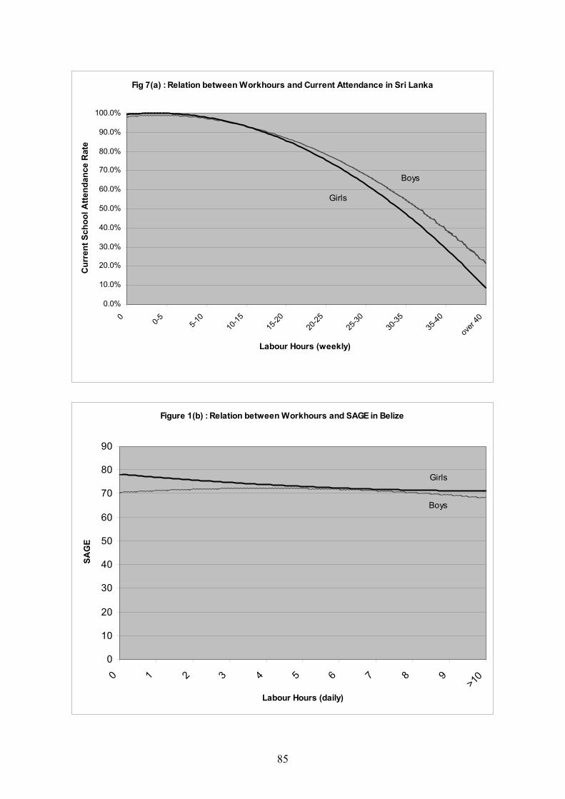
85

Fig 7(a) : Relation between Workhours and Current Attendance in Sri Lanka

0.0%

10.0%

20.0%

30.0%

40.0%

50.0%

60.0%

70.0%

80.0%

90.0%

100.0%

0 0-5 5-10

10-15

15-20

20-25

25-30

30-35

35-40

over

40

Labour Hours (weekly)

Cur

rent

Sch

ool A

ttend

ance

Rat

e

Girls

Boys

Figure 1(b) : Relation between Workhours and SAGE in Belize

0

10

20

30

40

50

60

70

80

90

0 1 2 3 4 5 6 7 8 9>10

Labour Hours (daily)

SAG

E

Boys

Girls

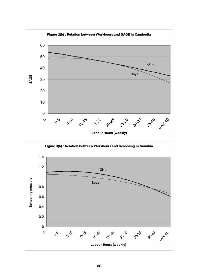
86

Figure 2(b) : Relation between Workhours and SAGE in Cambodia

0

10

20

30

40

50

60

0 0-5 5-10

10-15

15-20

20-25

25-30

30-35

35-40

over

40

Labour Hours (weekly)

SAG

E

Girls

Boys

Figure 3(b) : Relation between Workhours and Schooling in Namibia

0

0.2

0.4

0.6

0.8

1

1.2

1.4

00-5 5-1

010

-1515

-2020

-2525

-3030

-3535

-40

over

40

Labour Hours (weekly)

Scho

olin

g m

easu

re

Boys

Girls

87

Figure 4(b) : Relation between Workhours and SAGE in Panama

0

10

20

30

40

50

60

70

80

00-5 5-1

010

-1515

-2020

-2525

-3030

-3535

-40

over

40

Labour Hours (weekly)

SAG

E

Boys

Girls

Figure 5(b) : Relation between Workhours and Schooling in Philippines

0

0.5

1

1.5

2

2.5

3

3.5

4

4.5

00-5 5-1

010

-1515

-2020

-2525

-3030

-3535

-40

over

40

Labour Hours (weekly)

Scho

olin

g M

easu

re

Boys

Girls

88

Figure 6(b) : Relation between Workhours and Schooling in Portugal

0

0.5

1

1.5

2

2.5

3

3.5

00-5 5-1

010

-1515

-2020

-2525

-3030

-3535

-40

over

40

Labour Hours (weekly)

Scho

olin

g

Boys

Girls

Figure 7(b) : Relation between Workhours and SAGE in Sri Lanka

0

10

20

30

40

50

60

70

80

90

100

00-5 5-1

010

-1515

-2020

-2525

-3030

-3535

-40

over

40

Labour Hours (weekly)

SAG

E

Boys

Girls

89

Fig 8(a) : Relationship between mean study time and child ages in Sri Lanka

0

20

40

60

80

100

120

140

5 7 9 11 13 15 17Age

Stud

y M

inut

es (w

eekl

y)

don't workwork

Fig 8(b) : Relationship between mean study time and child age for Sri Lankan children who attend school

0

20

40

60

80

100

120

140

160

5 7 9 11 13 15 17Age

Stud

y M

inut

es (w

eekl

y)

don't workwork

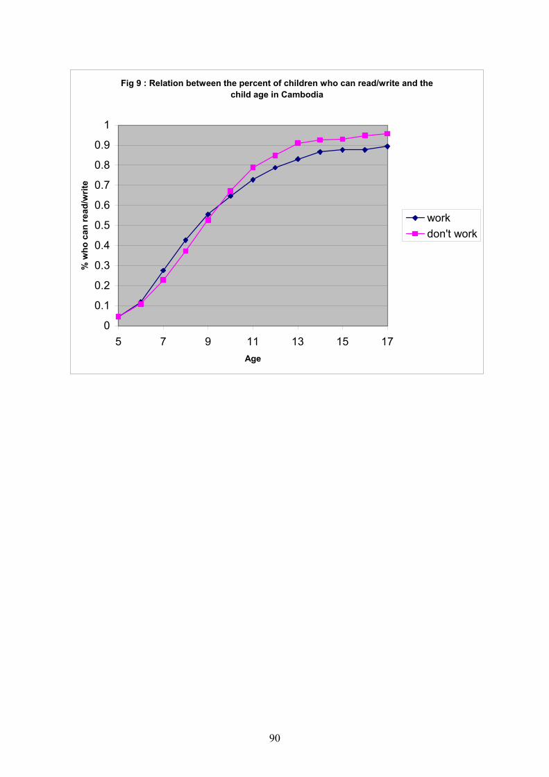
90

Fig 9 : Relation between the percent of children who can read/write and the child age in Cambodia

0

0.1

0.2

0.3

0.4

0.5

0.6

0.7

0.8

0.9

1

5 7 9 11 13 15 17Age

% w

ho c

an re

ad/w

rite

workdon't work

91

Economics Discussion Papers 2003-01 On a New Test of the Collective Household Model: Evidence from Australia, Pushkar Maitra

and Ranjan Ray

2003-02 Parity Conditions and the Efficiency of the Australian 90 and 180 Day Forward Markets, Bruce Felmingham and SuSan Leong

2003-03 The Demographic Gift in Australia, Natalie Jackson and Bruce Felmingham

2003-04 Does Child Labour Affect School Attendance and School Performance? Multi Country Evidence on SIMPOC Data, Ranjan Ray and Geoffrey Lancaster

2002-01 The Impact of Price Movements on Real Welfare through the PS-QAIDS Cost of Living Index for Australia and Canada, Paul Blacklow

2002-02 The Simple Macroeconomics of a Monopolised Labour Market, William Coleman

2002-03 How Have the Disadvantaged Fared in India? An Analysis of Poverty and Inequality in the 1990s, J V Meenakshi and Ranjan Ray

2002-04 Globalisation: A Theory of the Controversy, William Coleman

2002-05 Intertemporal Equivalence Scales: Measuring the Life-Cycle Costs of Children, Paul Blacklow

2002-06 Innovation and Investment in Capitalist Economies 1870:2000: Kaleckian Dynamics and Evolutionary Life Cycles, Jerry Courvisanos

2002-07 An Analysis of Input-Output Interindustry Linkages in the PRC Economy, Qing Zhang and Bruce Felmingham

2002-08 The Technical Efficiency of Australian Irrigation Schemes, Liu Gang and Bruce Felmingham

2002-09 Loss Aversion, Price and Quality, Hugh Sibly

2002-10 Expenditure and Income Inequality in Australia 1975-76 to 1998-99, Paul Blacklow

2002-11 Intra Household Resource Allocation, Consumer Preferences and Commodity Tax Reforms: The Australian Evidence, Paul Blacklow and Ranjan Ray

Copies of the above mentioned papers and a list of previous years’ papers are available on request from the Discussion Paper Coordinator, School of Economics, University of Tasmania, Private Bag 85, Hobart, Tasmania 7001, Australia. Alternatively they can be downloaded from our home site at http://www.utas.edu.au/economics