Embed Size (px)
Citation preview

NBER WORKING PAPER SERIES
SCHOOL REOPENINGS, MOBILITY, AND COVID-19 SPREAD:EVIDENCE FROM TEXAS
Charles J. CourtemancheAnh H. Le
Aaron YelowitzRon Zimmer
Working Paper 28753http://www.nber.org/papers/w28753
NATIONAL BUREAU OF ECONOMIC RESEARCH1050 Massachusetts Avenue
Cambridge, MA 02138May 2021
We thank SafeGraph, Inc. for making their data available for research. We also thank Jessica Thomas, Hunter McCormick, Ben Scott, and Yaxiang Song for collecting school districts start dates and modality of instruction from web searches. Finally, we thank Dan Goldhaber, Joe Sabia, Richard Buddin, and seminar participants at the Frank Batten School of Leadership and Public Policy and the School of Education and Human Development at the University of Virginia for helpful comments. The views expressed herein are those of the authors and do not necessarily reflect the views of the National Bureau of Economic Research.
NBER working papers are circulated for discussion and comment purposes. They have not been peer-reviewed or been subject to the review by the NBER Board of Directors that accompanies official NBER publications.
© 2021 by Charles J. Courtemanche, Anh H. Le, Aaron Yelowitz, and Ron Zimmer. All rights reserved. Short sections of text, not to exceed two paragraphs, may be quoted without explicit permission provided that full credit, including © notice, is given to the source.

School Reopenings, Mobility, and COVID-19 Spread: Evidence from TexasCharles J. Courtemanche, Anh H. Le, Aaron Yelowitz, and Ron ZimmerNBER Working Paper No. 28753May 2021JEL No. I18,I28
ABSTRACT
This paper examines the effect of fall 2020 school reopenings in Texas on county-level COVID-19 cases and fatalities. Previous evidence suggests that schools can be reopened safely if community spread is low and public health guidelines are followed. However, in Texas, reopenings often occurred alongside high community spread and at near capacity, making it difficult to meet social distancing recommendations. Using event-study models and hand-collected instruction modality and start dates for all school districts, we find robust evidence that reopening Texas schools gradually but substantially accelerated the community spread of COVID-19. Results from our preferred specification imply that school reopenings led to at least 43,000 additional COVID-19 cases and 800 additional fatalities within the first two months. We then use SafeGraph mobility data to provide evidence that spillovers to adults’ behaviors contributed to these large effects. Median time spent outside the home on a typical weekday increased substantially in neighborhoods with large numbers of school-age children, suggesting a return to in-person work or increased outside-of-home leisure activities among parents.
Charles J. CourtemancheDepartment of EconomicsGatton College of Business and Economics University of KentuckyLexington, KY 40506-0034and [email protected]
Anh H. LeDepartment of EconomicsGatton College of Business and Economics University of KentuckyLexington, KY [email protected]
Aaron YelowitzUniversity of KentuckyDepartment of Economics225H Business and Economics Building Lexington, KY [email protected]
Ron ZimmerUniversity of KentuckyMartin School of Public Policy and Administration Patterson Office Tower 423Lexington, KY [email protected]

2
I. Introduction
The COVID-19 pandemic has led to gut-wrenching decisions about whether and when to
open schools for in-person instruction. Ideally, these decisions would be made from an evidence-
based cost-benefit analysis. However, initially there was very little evidence to make these
decisions, and only recently has more information become available. On the benefit side, recent
research suggests that remote learning leads to significant learning loss, especially among
disadvantaged populations (Kuhfeld et al., 2020; Kuhfield and Tarasawa, 2020; Maldonado and
Witte, 2020). Remote learning also could lead to delayed social and emotional development and
reduced detection of child abuse as teachers are often at the front lines of detection (Schmidt and
Natanson, 2020). In addition, remote learning could lead families to make difficult decisions
between working and staying home with young children, which could dampen the speed of the
economic recovery (Green et al, 2020; Council of Economic Advisers, 2020). Together, this
suggests that opening schools could improve student learning and social and emotional
development while minimizing the possibility of child abuse.
On the cost side, there are concerns of health risks for students, staff, and the larger
community as the openings could further spread COVID-19. These concerns have been
championed by teacher unions, which argue that schools should open only when they are safe
(Hurt, Ball, and Wedell, 2020). However, a Centers for Disease Control and Prevention (CDC)
report examining 17 rural Wisconsin schools using contact tracing found minimal transmission
both within and outside of the schools (Falk et al., 2021). Other investigations of known cases
among students and staff – such as Doyle et al.’s (2021) study of Florida and Emily Oster’s K-12
COVID-19 dashboard – tend to reach similar conclusions.1 Accordingly, the CDC recently
1 Oster’s dashboard is available at https://covidschooldashboard.com/.

3
concluded that in-person instruction can be carried out safely as long as masks are worn, social
distancing is maintained, community spread is low, and other community restrictions (e.g., on
restaurants) remain in place (Honein et al., 2021).
However, contact-tracing-based evidence alone is insufficient to fully understand the
health implications of reopening schools. Contact tracing is widely known to be inadequate in the
U.S. due to insufficient staff and resources to keep up with large numbers of new cases, as well as
resistance to provide information among those contacted. For instance, a National Public Radio
story found that 27 percent of cases and 43 percent of contacts lacked phone numbers in Delaware,
only 44 percent of new cases were reached within 24 hours in New Jersey, and only 4.5 percent
and 25 percent of cases could be traced to known contacts in Washington, D.C. and Delaware,
respectively (Simmons-Duffin, 2020). Moreover, econometric evidence from Dave et al. (2020)
linked more than 100,000 cases to the Sturgis Motorcycle Rally in South Dakota, compared to just
328 identified by contact tracing. This illustrates the potential for contact tracing to substantially
underestimate the total number of cases resulting from a particular event after several rounds of
exponential spread. One missing link in the contact tracing chain prevents the attribution to the
event of any people infected by the missing link, any people those people subsequently infected,
and so on.
On the other hand, the number of known cases resulting from in-school spread could
overstate the net increase in the number of cases, as it does not account for the counterfactual
activities students and staff would be engaging in if schools were closed. While some students and
staff would stay at home and face little risk, others would go to day care facilities, parks,
restaurants, virtual school pods at friends’ houses, or other places where adherence to mitigation
measures could be lower than in schools (Courtemanche et al., 2020).

4
Additionally, focusing only on net changes in risk among those attending school misses a
potentially important part of the story: spillover effects on the behaviors of parents or others in the
community. Kids returning to in-person school may allow parents or other caregivers to return to
in-person work or outside-the-home activities, leading to COVID-19 spread in the community
even if there is minimal spread in the schools. Spillovers could even extend beyond families
directly affected by the return to school, as school openings could signal to the community that it
is safe to return to normal activities, again fueling spread (Glaeser et al., 2020). Alternatively,
spillovers could reduce spread if people foresee danger from school reopenings and cut back on
other activities.
Econometric studies can provide answers to these debates by estimating reduced-form
effects that encompass all mechanisms through which reopening schools influences the spread of
COVID-19. Three concurrent working papers examine the effects of school openings in Germany
(Isphording et al, 2021), Michigan and Washington (Goldhaber et al., 2021, hereinafter we refer
to as CALDER study) and the U.S. as a whole (Harris et al., 2021, hereinafter we refer to as Tulane
study). While the current versions of these studies find little evidence that reopening schools
increases COVID-19 spread on average, the Tulane and CALDER studies find some evidence that
this may not be the case in communities with high levels of preexisting transmission.
The above discussion highlights a key distinction: the consensus that schools can open
safely with low community spread and proper safeguards is not the same as saying that all schools
are opening safely. To examine what can happen in a less idealized scenario, we focus on the state
of Texas. All of the school districts in Texas reopened for in-person instruction at some point
during the 2020 fall semester. Many did so when COVID-19 rates in the community were

5
relatively high, generally without staggered or hybrid strategies to limit the number of students
attending at one time.
We estimate the impact of school reopenings in Texas on COVID-19 spread using hand-
collected information on school districts’ instructional modality and start dates combined with
weekly county-level data on confirmed COVID-19 cases and fatalities. Our baseline model is an
event study that separately estimates effects for each week in a four-month bandwidth surrounding
reopenings. This allows us to assess pre-treatment trends while also allowing impacts to emerge
gradually due to incubation periods, testing delays, multiple rounds of subsequent spread, and the
fact that COVID-19 deaths tend not to occur quickly. We find that school reopenings in Texas
gradually but substantially increased the per capita numbers of new weekly COVID-19 cases and
deaths. To illustrate, 95 percent confidence intervals from the baseline regression imply that school
reopenings across Texas led to at least 43,000 additional COVID-19 cases and at least 800
additional fatalities after two months. These magnitudes represent 12 percent and 17 percent,
respectively, of the total numbers of cases and deaths in the state during that period. Results are
qualitatively similar across a wide range of robustness checks, including those that address newly
discovered issues with staggered-treatment-time two-way-fixed-effects research designs. Using
similar event-study models and SafeGraph data (which tracks the movement of individuals aged
16 and older by using cell phone data), we show that time spent outside the home by adults rose
sharply in communities with the largest numbers of children after school reopenings. Some
evidence also suggests increased mobility in communities with large numbers of seniors,
consistent with signaling effects on those not directly affected by the reopenings.
Overall, we find convincing evidence that opening schools led to community spread, and
was likely facilitated by increased mobility, which could arise both directly in schools but also
6
indirectly through the behaviors of parents or other adults. Although the recent distribution of
effective vaccines is changing the cost-benefit of the calculations policymakers are making,
difficult decisions about schools will likely continue into the 2021-2022 academic year. Children
under sixteen years old cannot yet be vaccinated, there are broad geographic pockets across the
country with low adult vaccination rates, and the emerging variant B.1.1.7 infects children more
easily than prior strains. 2,3
II. Background
School Reopenings in Texas
On July 7, 2020, the Texas Education Agency (TEA) issued school reopening guidelines,
which covered topics such as COVID-19 prevention, responses, mitigation, and information
dissemination.4 These guidelines covered the wearing of masks, reporting of positive cases, and
screening of staff, teachers, and students. Most importantly, it provided the following guidance for
reopening schools: “during a period up to the first four weeks of school, which can be extended by
an additional four weeks by vote of the school board, school systems may temporarily limit access
to on-campus instruction.”
These instructions were further clarified by a July 17, 2020 joint statement from Governor
Greg Abbot, Lt. Governor Dan Patrick, Speaker Dennis Bonnen, Senate Education Chairman
Larry Taylor, and House Education Chairman Dan Huberty. They stated that local school districts
have the constitutional authority to decide when and how schools safely open and noted that local
school boards have the authority to set the start date which could be in in “August, September, or
2 https://health.usnews.com/health-care/patient-advice/articles/when-will-there-be-a-covid-19-vaccine-for-kids 3 https://www.nydailynews.com/coronavirus/ny-covid-variants-michael-osterholm-new-york-20210404-73bhzmgpzremnpr5hirw2eo724-story.html 4 https://www.wfaa.com/article/news/education/texas-students-must-wear-face-masks-at-school-tea-says/287-e2ef67ef-6ec7-4827-9a80-43fb83932564

7
even later.”5 They also noted that local school boards can make these decisions “on advice and
recommendations by local public health authorities but are not bound by those recommendations.”
Importantly, the statement also clarified that not only could school districts start the first four
weeks as a “back to school transition” with remote instruction, but school districts could extend
their back-to-school transition an additional four weeks with a vote of the school board and a
waiver from the state. After eight weeks, school districts could ask for an addition extension as the
result of health concerns related to COVID-19 and the TEA will decide those requests on a case-
by-case basis. Finally, the guidance from TEA noted that school districts must provide the option
for families of remote instruction, even if the school district provides in-person instruction.
However, because of the challenges of the logistics of providing both in-person and remote
instruction, school districts could restrict families to switching their choice of instructional
modality only at the end of grading periods.
With this policy context as background, Figure 1 displays the start date of opening schools
for in-person instruction for school districts in the 2020-21 school year relative to the start date of
opening schools in the 2019-20 school year.6 About two-thirds of school districts opened schools
in 2020-21 within one week of the start date of 2019-20 in spite of the widely documented surge
in COVID-19 cases in Texas in the summer of 2020. Moreover, less than two percent of school
districts delayed the reopening by more than eight weeks, possibly because of the requirements
imposed by the state to obtain an exemption to remain virtual longer than eight weeks. To the
5 https://gov.texas.gov/news/post/governor-abbott-lt-governor-patrick-speaker-bonnen-chairman-taylor-chairman-huberty-release-statement-on-school-re-openings 6 In most districts, we were able to determine the 2019-20 start date. However, in the cases where we were not able to identify the 2019-20 start date we either used the prior year start date (e.g., 2018-19) or the median 2019-20 start date within the county.

8
extent that state directives trumped local caseloads or politics in influencing reopening decisions,
that would help to alleviate endogeneity concerns in our econometric analysis.
Econometric Evidence on Schools and COVID-19
As the pandemic began to unfold during the spring of 2020, very little was known about
the likelihood of spread among young populations and whether schools could safely operate with
in-person instruction. Three early studies that controlled for other accompanying restrictions like
restaurant closures and shelter-in-place orders did not find evidence that school closings slowed
the spread of COVID-19 (Courtemanche et al., 2020; Hsiang et al., 2020; Flaxman et al., 2020).
However, a fourth study that did not control for these other restrictions did find evidence of a
sizeable effect (Auger et al., 2020). These prior studies are of limited usefulness for reopening
decisions as almost all the spring school closures in the United States occurred within one week
of each other, leading to little identifying variation and generally imprecise estimates. While
controlling for other types of restrictions is important for causal inference, it further strains the
available identifying variation, perhaps explaining the null findings from studies that did so.
Further, it is not clear that closings and openings should have symmetric effects. Much more was
known about mitigation strategies in fall 2020 compared to spring, but community spread was also
much greater in the fall.
Only recently has econometric evidence on reopening schools begun to emerge. Isphording
et al. (2020) leveraged variation in the timing of school start dates and found little evidence of
effects on community spread in Germany.7 However, the relevance of this finding for a U.S.
population with different attitudes toward COVID-19 and different mitigation policies, both inside
7 This result is consistent with two descriptive studies of small sets of schools in France and Helsinki that also found little evidence of spread (Dub et al., 2020; Fontanet et al., 2020).

9
and outside of schools, is unclear. Tulane researchers used national insurance claims data and U.S.
Department of Health and Human Services (HHS) hospitalization data along with national data on
school reopenings to examine the impact of school reopenings on hospitalization (Harris et al.,
2021). Overall, they found no association between school reopenings and hospitalization.
However, they noted that in areas with higher pre-opening COVID-19 hospitalization rates, the
results are less conclusive with some evidence indicating that in these areas, school openings could
lead to greater hospitalizations. Given that the data for the study was only collected through mid-
fall 2020—prior to much of the national surge of hospitalizations—the study’s findings do not
necessarily extrapolate to later in the pandemic. Moreover, the sample period only allows for six
weeks of post-treatment data, which may not be enough time for meaningful increases in
hospitalizations to occur given incubation periods and the potential need for multiple rounds of
spread outward from schools before reaching the vulnerable individuals who are most likely to
require hospitalization.
Another study, released by a research consortium named CALDER, examined monthly
county level COVID-19 cases using school reopening information provided by Michigan and
Washington’s departments of education (Goldhaber et al., 2021). The researchers noted that in
Washington, only 10 percent of districts (almost entirely rural) and only 2 percent of the student
population was attending either a school operating with hybrid or in-person instruction. In
Michigan, the percentages were higher, with 76 percent of schools operating either with hybrid or
in-person instruction. Like the Tulane study, this study examined COVID-19 cases prior to much
of the surge of cases in the winter of 2020-21. The research team found that in-person modality
options are not associated with increased spread of COVID-19 at low levels of pre-existing
COVID-19 cases but did find that cases increase at moderate to high pre-existing COVID-19 rates.

10
Again, the analysis raises questions as to which set of results are more relevant to the COVID-19
conditions of the winter.
We complement these other concurrent studies by examining a state where conditions may
have been less than ideal for a safe reopening. First, Texas had relatively high rates of COVID-19
spread in early fall of 2020 that roughly mirrored the national conditions that would emerge toward
the end of the semester. To illustrate, Figure 2 shows weekly COVID-19 cases per 100,000
residents in Texas compared to Washington, Michigan, and the U.S. as a whole during the latter
half of 2020. The vertical lines delineate the weeks of June 20 through October 16 – a four-month
period centered on the modal reopening date in our Texas data, and a similar period to that used in
the Tulane and CALDER studies. Texas’ rate of new cases was substantially greater than those of
Washington, Michigan, and the overall U.S. during early fall when the bulk of Texas’ schools
reopened for in-person instruction.
Additionally, many states opened schools using hybrid models where only partial numbers
of students attended schools each day to allow for greater social distancing. In contrast, most Texas
schools opened at near capacity. For instance, in reviewing school opening plans of Texas school
districts, our best estimate is that over 90 percent of school districts opened fully in-person without
any staggered or phased-in attendance. This is in contrast to 42 percent nationally (Harris et al.,
2021). In addition, using Texas’ Department of State Health Services data on the proportion of
students attending in person by late September, we found that out of the 1,049 school districts, 358
had over 90 percent of their students attending in person with 27 having 100 percent.8 Moreover,
studies have shown that residents of politically conservative areas – such as the majority of Texas
– are less likely to follow social distancing and mask-wearing recommendations than those in
8 https://dshs.texas.gov/coronavirus/schools/texas-education-agency/. We excluded charter schools from the analysis.

11
politically liberal areas (Milosh et al, 2020). This could influence the impact of reopening schools
on COVID-19 spread in several ways, possibly including weaker enforcement of guidelines at
schools and extracurricular activities, greater increases in mobility among parents, a stronger
signal to the community that life can return to normal, and less willingness to impose compensatory
other aspects of life.
The Texas context offers other advantages as well. Texas allowed districts more discretion
in when to open schools than many other states, allowing us to examine the effect of variation in
timing of school openings in the context of common statewide mitigation policy, thereby reducing
the possibility of omitted variable bias from other restrictions.9 In addition, in contrast to the
Tulane and CALDER studies, which observed only a portion of schools open, every school district
in the state eventually opened schools during the time frame of our study. This allows for an
examination of wide-ranging school districts including rural and urban, large and small, and non-
diverse and racially diverse. In the CALDER and Tulane studies, open schools were
disproportionally rural. Finally, Texas has a large number of school districts and counties, which
provides statistical power to detect effects. As a source of comparison, while Texas has 254
counties and 1,049 school districts,10 Michigan has 83 counties and 810 school districts and
Washington has 39 counties and 286 school districts.
III. Data
To collect information for each school district’s start date and modality, we performed
Google searches in which a team of assistants searched for key terms using district name and the
9 Restrictions can vary within states, but we were unable to find any instances of cities or counties in Texas imposing or eliminating policies like shelter-in-place orders or mask mandates during our sample period. 10 One county (Loving) has no schools within the county.

12
phrase “back to school plan”.11 The vast majority of districts had a back-to-school plan and it often
included both the district’s modality plan for instruction and the school district start date. If the
school district started with virtual instruction, the back-to-school plan often listed the planned date
for in-person instruction.12 In cases in which the start date was not listed, the team of assistants
searched for the school district’s academic calendar. In cases where back-to-school plans or
calendars were not available, we also conducted newspaper and Facebook searches to identify this
information through news stories and school district’s Facebook posts.13 Even in cases where a
back-to-school plan and/or academic calendars were available, we often conducted additional
newspaper or Facebook searches to verify the district’s start date and modality of instruction.
Because COVID-19 cases and fatalities are only available at the county level, we need to
aggregate the school reopening variable from the district to the county level, which requires
accounting for the fact that not all districts within a county opened at the same time. In the Tulane
study, the researchers defined treatment as occurring when the first district within a county
reopened. However, for many districts in Texas, this definition would result in a county being
labeled “treated” when only a small fraction of schools is actually open. Consider Bexar County,
a large county that includes San Antonio. Southwest Independent School District (ISD), which
11 Like the Tulane study, we did not include charter or private schools primarily because they represent a small minority of the total students in the states and also because it would have been difficult to ascertain this information. 12 In some cases, districts phased in in-person attendance (e.g., Kindergarten through 3rd grade could attend in person one week and the following week the rest of the grades could attend in person). In these cases, we used the first date students were allowed on campus. If the district only allowed special education students on campus, we did not count this as in-person instruction given the small number of students on campus. 13 After these steps, there were only 11 school districts in which we could not identify the start date and only 17 school districts we could not identify the modality of instruction. We tried to follow up with each district with a phone call. Through these phone calls, we were able to identify the start date for seven of the 11 missing dates for school districts and the missing modality information for 12 of the 17 school districts. Therefore, we had missing dates for four school districts, which we imputed based on the median start date within their county. For modality, we had missing dates of five school districts, which we imputed as the majority instructional modality of the school districts within the county. These are very small districts, with the average size of the missing start date districts being 78 students and the average size of the districts with missing modality information being 177 students. Since our data will be population-weighted, these districts are effectively inconsequential to the results.

13
represents less than 5 percent of the county’s student enrollment, was the first district to open
schools on August 24, 2020. However, there were some districts within the county that opened up
schools as late as seven weeks later and six school districts representing 75 percent of the county’s
student population opened on September 8, 2020. In this case, defining treatment based on the
earliest opening school district would effectively lead to it being assigned two weeks too early
relative to the most consequential shock. Therefore, our primary treatment definition is the week
in which the county had the largest jump in percentage of county students who could attend a
school in person. In the case of Bexar County, that would be the week of September 8th.14 We
should also note that treatment begins for our empirical analysis once schools open for any type
of in-person instruction including fully in-person, phased-in (e.g., a subset of grades open for in-
person instruction with gradual number of grades eligible to attend in-person over time), or as a
hybrid model (e.g., students attending in person part of the week and attending virtually the rest of
the week). However, as discussed previously, phased-in and hybrid reopenings were rare in Texas.
It should also be noted that in opening schools for in-person instruction, districts almost
uniformly allowed families to choose to attend in-person or remotely. However, districts had to
prepare for the possibility that all or nearly all students could attend in person. Therefore, our main
treatment variable could be thought of as “intent-to-treat” (ITT) analysis as a district’s decision to
provide in-person instruction is providing the opportunity for all students to attend in person. That
said, schools in Texas tended to open at relatively close to full capacity as nearly 60 percent of all
school districts had 80 percent or more of their students enrolled for in-person instruction by the
end of September. Our analysis is also an ITT analysis in a second way. Once treatment begins by
14 Later, we present a series of analyses that suggests our results are robust to alternative definitions of treatment including using the first school district that opened schools in person, 50 percent of the county enrollment is open for in-person instruction, and 20 percent of the county enrollment is open for in-person instruction.

14
a school district opening schools for in-person instruction, we consider the school opened
throughout the analysis, even if the school has a temporary shutdown as a result of an outbreak. In
defining treatment in this way, our estimates should be seen as conservative estimates.
Our COVID-19 data come from the Texas Department of State Health Services
(TDSHS).15 Numbers of COVID-19 cases, fatalities, and tests are recorded daily at the county
level from May 3, 2020 through January 3, 2021. We use weekly (Sunday through Saturday) data
instead of daily data because not all labs are open daily or do not report daily (e.g., many labs are
not open on weekends) and can have duplicate numbers or reporting errors, which can lead to
oscillating numbers from one day to the next. By using weekly numbers, we are largely able to
smooth out these fluctuations.16 To account for variations in county population, we calculated
COVID-19 cases, fatalities, and tests per 100,000 residents using 2019 county population estimates
from the Census Bureau.17 These cases and fatalities variables will be our main outcome variables,
while the testing variable will be a control in the cases regressions.
To help understand potential spillover effects of school reopenings on adult mobility, we
utilize Social Distancing Metrics (Version 2.1, “SDM”) data provided by SafeGraph, Inc., from
May 3, 2020 to January 3, 2021.18 SafeGraph collects information on almost 45 million cellular
phone users, including about 10 percent of devices in the U.S. The sample correlates very highly
with the true Census populations with respect to distribution by county, educational attainment,
15 https://dshs.texas.gov/coronavirus/additionaldata.aspx 16 It should be noted that some data errors within the TDSHS data systems have been discovered over time as documented by media accounts: https://www.khou.com/article/news/health/coronavirus/texass-record-high-covid-positivity-rate-falls-after-data-experts-investigate/287-ffc19167-0d47-4be9-8c06-8648229288ef and https://www.texastribune.org/2020/09/24/texas-coronavirus-response-data/. Corrections to these errors could cause accumulated cases or tests to decrease over time as the data are corrected. These anomalies should create noise, but not bias and should largely be accounted for in our analysis using week fixed effects. 17 https://www.census.gov/data/datasets/time-series/demo/popest/2010s-counties-total.html 18 https://www.safegraph.com/blog/stopping-covid-19-with-new-social-distancing-dataset

15
and income.19 These data are aggregated from GPS pings provided by cellular devices that have
opted-in to location sharing services from smartphone applications. The device data is aggregated
by Census Block Group (CBG) and day, based on a device’s “home” location.20 In our timeframe,
there were 15,705 CBG’s overall in the Texas SDM; on an average day, more than 1.9 million
devices were followed in Texas. For our analysis, we restricted the sample to a balanced panel of
14,580 CBG’s (with more than 1.6 million overall devices on an average day).21 The typical CBG
had approximately 112 devices. We created samples at the weekly level for the full week (Monday
through Sunday), for weekdays (Monday through Friday), and for weekends (Saturday and
Sunday).
We utilize four of the mobility measures provided in the SDM that are often used in other
studies. The most commonly used measure is the fraction of devices that do not leave their home
location during a given day (“Percent Completely Home”).22 We also use two “work” measures.
SafeGraph defines “work” as either the fraction of devices that spent more than 6 hours at a non-
home location between 8am-6pm (“Percent Full Time”) or fraction of devices that spent between
4-6 hours at a non-home location between 8am-6pm (“Percent Part Time”).23 Finally, several
19 https://www.safegraph.com/blog/what-about-bias-in-the-safegraph-dataset 20 To impute a “home” location for a cellphone user, SafeGraph considers a common nighttime location of each mobile device. In the entire United States, the SDM is aggregated to approximately 220,000 CBGs. To enhance privacy, CBG’s are excluded if they have fewer than five devices observed in a month. 21 CBG’s were excluded if (a) the CBG was not observed for all days in our sample period, (b) the CBG could not be merged to demographic information from the 2018 American Community Survey (ACS) 5-year estimates, (c) the CBG’s population – according to the 2018 ACS – was in the bottom or top 1 percent of the full distribution (corresponding to 391 and 7150, respectively), or (d) over the course of the panel, relative to the mean device count in the CBG, any specific CBG-day observation had a device count that more than twice the mean or less than half the mean. By restricting to CBG’s with relatively stable numbers of devices over the long panel, we hope to avoid complications related to installation and removal of apps, inactive devices, and sample attrition highlighted in some other studies (Andersen et al., 2020; Allcott et al., 2020). Although Safegraph reports that some apps implement GPS collection methods that depend on the movement of the device (rather than a fixed time interval), this would likely affect levels of certain metrics (e.g., completely home all day) but not changes. 22 See Bailey et al. (2020), Bullinger et al. (forthcoming), Cronin and Evans (2020), Allcott et al. (2020), Dave et al. (2020a), Simonov et al. (2020), Dave et al. (2021), Friedson et al. (Forthcoming), and Gupta et al. (2020). 23 See Bullinger et al. (forthcoming) and Simonov et al. (2020).

16
studies have examined median time spent away from home (or at home).24 These measures are
based on the observed minutes outside of home (or at home) throughout the day, regardless of
whether these time episodes are contiguous. The time during which a smartphone is turned off is
not counted towards the measures.
Finally, for some of our analyses, we utilize county-level variables from other sources. The
county’s college enrollment is available from the U.S. Department of Education National Center
for Educational Statistics (NCES).25 Percent of voters who voted for President Trump in the 2016
presidential election comes from the MIT Election and Data Science Lab (2018). We control for
average weekly temperature, precipitation, and snowfall using data collected by the National
Oceanic and Atmospheric Administration (NOAA) and the Global Historical Climatology
Network.
Our main analysis sample contains a balanced event-time window surrounding treatment,
i.e. the week of the county’s largest increase in percentage of students who can attend in-person
school. For the COVID-19 outcomes, we include eight weeks prior to treatment, the treatment
week, and eight weeks after treatment. A lengthy post-treatment period allows for multiple rounds
of spread (e.g. from student to parent to grandparent), incubation periods, time to receive and
obtain results from a test, and the fact that deaths can occur weeks after infection. On the other
24 See Allcott et al. (2020), Dave et al. (2020a), Cotti et al. (forthcoming), and Gupta et al. (2020). 25 These data were collected at http://nces.ed.gov/ccd/elsi/.The reporting years of enrollment ranged from 2013-2017. As part of the data cleaning process, for residential campuses only, we assumed all enrolled students could attend classes in person and therefore, we calculated the maximum weekly proportion of the total county population that could be on campus by dividing the number of enrolled students by the county population. To calculate the daily proportion of college students of the total county population, we assumed that no students were on campus during the summer (nearly all colleges did online instruction over the summer). We also assumed all residential colleges had in-person classes for the fall semester. For those colleges with no residential students, we assumed the colleges were providing instruction either online or had minimal student interactions. Using Google searches of academic calendars, we identified the start date for each college, which is the day we assumed students began interacting on campus. In many counties, there are multiple colleges with different start dates, which means the college proportion changes over time as more and more colleges start their fall sessions.

17
hand, a long post-treatment period faces a relatively high risk of confounding from other
concurrent shocks. In our case, the holiday break – which started in many Texas districts after the
week of December 13 – is a particular concern, as schools being “reopened” should not influence
spread when they are not in session. In our view, an eight week post-treatment window best
balances these considerations. It is long enough to plausibly capture much of the dynamics of the
treatment effect. At the same time, it is short enough to avoid sample windows that stretch past the
week of December 13 for all but two small counties (Starr and Zavala) that will have little influence
in our population-weighted sample. For the SafeGraph mobility outcomes, there is not a clear
reason to expect a lag before treatment effects emerge, so we limit the event-time window to six
weeks on each side, thereby ensuring that the sample window does not extend past the week of
December 13 for any county.
Table 1 shows means and standard deviations for our outcome variables in both the pre-
and post-treatment periods, weighted by population. Interestingly, new cases per capita were about
the same in the pre- and post-treatment periods, while death rates went down by almost 50 percent.
This was in spite of a moderate increase in mobility across all four measures. Of course, numerous
factors affect these flat or downward trends, including better understanding of preventive measures
such as mask-wearing, advancements in treatments, and the average age of cases gradually
becoming younger. A finer-grained econometric analysis is necessary to disentangle the causal
effects of school reopenings from these underlying trends.
Table 2 shows results from a simple cross-sectional regression of week of reopening
(ranging from 14 to 28, with week 1 being the week of May 3) on several county-level variables
that might be expected to influence reopening decisions: President Trump’s 2016 vote share,
percent Hispanic, percent Black, county population, and percent of the SafeGraph sample who

18
stayed completely at home for the day in the four weeks prior to any schools reopening (a proxy
for compliance with public health guidelines), and average weekly new cases per capita in the four
weeks prior to any schools reopening. We standardize the covariates to allow a direct interpretation
of the magnitudes. Trump vote share is the dominant predictor, which is consistent with previous
research that showed politics drove school opening decisions (Valant, 2020). Each standard
deviation increase in Trump vote share is associated with schools reopening 1.22 weeks sooner. In
contrast, none of the other variables are statistically significant, and none have a magnitude greater
than 0.17 weeks. The coefficient for pre-school-year caseloads is nearly zero, and its p-value is
nearly 0.9. Therefore, reopening decisions appear to have been driven much more heavily by
politics than public health considerations, which may be surprising but is consistent with prior
research (Valant, 2020). This can be seen as favorable for an econometric analysis, as it suggests
that reverse causality from caseloads influencing reopening decisions should not be a concern. We
will be able to account for stable county characteristics such as political views by including county
fixed effects.
IV. Econometric Methods
We aim to identify the causal effects of school reopenings on new weekly COVID-19 cases
and fatalities per 100,000 residents by estimating event-study regression models of the form
𝑦𝑦𝑐𝑐𝑐𝑐 = 𝛽𝛽0 + � 𝛽𝛽1𝑖𝑖
8
𝑖𝑖=−8,𝑖𝑖≠−1
𝑂𝑂𝑂𝑂𝑂𝑂𝑂𝑂𝑐𝑐,𝑐𝑐−𝑖𝑖 + 𝛽𝛽2 𝑇𝑇𝑂𝑂𝑇𝑇𝑇𝑇𝑇𝑇𝑐𝑐𝑐𝑐 + 𝛼𝛼𝑐𝑐 + 𝜏𝜏𝑐𝑐 + 𝜀𝜀𝑐𝑐𝑐𝑐 (1)
where the subscripts c and t represent county and week; y is the case or fatality outcome; 𝑂𝑂𝑂𝑂𝑂𝑂𝑂𝑂
is the reopening indicator; 𝑇𝑇𝑂𝑂𝑇𝑇𝑇𝑇𝑇𝑇 is a control variable for the number of COVID-19 tests per

19
100,000 residents,26 included since differential testing rates across locations and time can be an
important driver of confirmed case numbers; 𝛼𝛼 and 𝜏𝜏 are county and time fixed effects; and 𝜀𝜀 is
the error term. Observations are weighted by county population, and standard errors are robust to
heteroskedasticity and clustered by county.
The summation term for the treatment variable reflects the inclusion of separate indicator
variables for whether schools will reopen eight weeks after week t, seven weeks after, six weeks
after, etc., down to two weeks after; whether schools reopened exactly in week t; and whether
schools reopened one week before week t, two weeks before, etc., up to eight weeks before. The
variable for whether schools will reopen one week from now is omitted as the reference period.
The “lead” terms (weeks until school reopening) measure pre-treatment trends, while the “lag”
terms (weeks after school reopening) measure the evolution of the treatment effects over time. As
discussed above, we expect the effects on new cases to grow over time because of the incubation
period, the lag between symptom onset and receiving a test, the time required to obtain test results,
and the exponential nature of case growth. For fatalities, we expect an even longer lag since deaths
typically occur after an extended battle with the illness.
We also estimate a number of variants of our baseline event-study specification as
robustness checks. The first three checks add variables in an effort to address possible omitted
variable bias concerns. Causal inference in our event-study model requires the assumption that
case and death trajectories would have evolved similarly in early versus late reopening counties in
the counterfactual in which schools did not reopen. The pre-treatment trends estimated using the
lead terms in the event-study model are informative as to how case and death trajectories would
26 Since test results might not be recorded in the same week that the test was conducted, we experimented with including lags of the testing variable, finding that the contemporaneous value as well as two weekly lags were statistically significant. We therefore include all three of those variables in the regressions.

20
have evolved in the counterfactual scenario. However, it is possible that some confounders did not
emerge until the post-treatment period. For instance, most Texas colleges and universities opened
for in-person instruction at the start of the fall semester. If these post-secondary reopenings fueled
COVID-19 spread and if school reopening dates were also systematically correlated with the
prevalence of college students in the county, this could bias our estimators for the school reopening
coefficients. We therefore estimate a model that controls for college and university reopenings in
a dose-response, event-study manner. Specifically, we construct a variable for the proportion of a
county’s population that attends an in-session post-secondary institution in a given week. We then
interact this continuous “dosage” measure with indicators for each of the eight weeks before and
after the first college reopening in the county. Our second robustness check controls for time-
varying unobservables more generally by including linear county-specific time trends.
For our third check, recall that the results from Table 2 showed that vote share for President
Trump was the dominant predictor of reopening week. Residents’ political views are presumably
fixed during a two-month sample period, meaning that they are captured by the county fixed
effects. However, it is possible that political views could influence not only levels of new COVID-
19 cases but also trends, and county fixed effects alone would not account for the latter. If heavily
Republican counties opened schools relatively early and also developed steeper COVID-19
trajectories in the fall for reasons besides school reopenings, our estimated effects of reopenings
would be biased upwards. We therefore estimate a model that adds interactions of time-invariant
Trump vote share with each week fixed effect, thereby flexibly allowing for right- and left-leaning
counties to have different COVID-19 trajectories.
The next series of robustness checks utilize alternate constructions of the key variables.
First, instead of defining reopening as occurring in the week with the largest increase in the

21
percentage of a county’s students who attend schools that reopened for in-person learning, we use
the week during which the county (a) crossed over the 50 percent threshold for students attending
reopened schools, (b) crossed over the 20 percent threshold, and (c) had its first reopening. The
latter is the treatment definition used by the Tulane study. Next, two checks consider alternate
functional forms for the case and fatality outcomes: (a) exponential growth rate in cumulative cases
(computed as the difference in the natural logs of cumulative cases from one week to the next) and
(b) the natural log of the count of new cases.
Our next two checks vary the way in which we control for COVID-19 testing, since
changes over time in the number of tests performed could be endogenous to the trajectory of new
infections. First, we simply drop the testing variables. Second, we control for the number of new
negative tests per 100,000 residents rather than total tests, as those might arguably reflect availably
of tests rather than level of virus in the community.27
The next group of robustness checks varies sample construction. Two checks shorten the
sample window from eight weeks on each side of treatment to six and four, respectively. Next, we
test whether the results could be driven by a small number of unusual counties by dropping (a) the
county of El Paso, which experienced dramatically more COVID-19 spread than any other county
in Texas during our sample period, and (b) all six counties with more than a million residents.
Finally, we consider a different way to ensure that the results are not driven exclusively by large,
urban areas by re-estimating the baseline model without weighting observations by county
population, thereby making the estimates reflective of effects in the average county (with each
county counting equally), as opposed to average effects across Texas as a whole. We also examine
27 Note that, since we did not control for testing in the baseline fatalities regression, we do not perform the robustness checks involving testing for that outcome.

22
the robustness of the findings by re-estimating the main model leaving out one county at a time,
for the six largest counties with population exceeding one million.
Finally, an emerging literature documents problems with two-way fixed-effects (TWFE)
models with staggered treatment times.28 First, TWFE regressions give more weight to
observations treated in the middle of the sample period, which can lead to unreliable estimates of
the average treatment effect if treatment effects are heterogeneous. Using the event-study
formulation with a balanced panel and a sample period centered around treatment time rather than
calendar time alleviates this concern. Since each county has exactly eight pre-treatment
observations, one observation during the treatment week, and exactly eight post-treatment
observations, the variance of each treatment variable is identical for each county.
More troublesome in our context is that, in settings that rely exclusively on variation in
treatment timing for identification as opposed to having control units, two-way fixed effects
models implicitly use early treated units as controls for later treated units. This leads to bias when
treatment effects are dynamic because the response of the early treated units is still evolving at the
time that they are called upon to be controls, effectively leading to a violation of the parallel trends
assumption for those particular late-versus-early comparisons. Event-study models do not
necessarily alleviate this concern. Under the assumption that the treatment effect either strengthens
or stays the same over time, the bias is toward zero and we can conclude that, if anything, our
estimates are conservative. We find this assumption plausible for COVID-19 outcomes; as
discussed above, all the reasons to expect treatment effects to evolve over time point towards them
becoming stronger rather than weaker.
28 This literature includes Callaway and Sant’ Anna (forthcoming), de Chaisemartin and D’Haultfoeuille (2020), Goodman-Bacon (forthcoming), and Sun and Abraham (2020). Our discussion in the remainder of this section is based on reviews of this emerging literature by Baker et al. (2021) and Cunningham (2021, pp. 461-510).

23
Nonetheless, we conduct two robustness checks that utilize newly developed methods that
address this issue. Both of these methods perform well in simulations and applications conducted
by Baker et al. (2021). First, we employ the “stacked regression” strategy used by Cengiz et al.’s
(2019) study of four decades of state minimum wage increases. This method begins by
constructing new datasets for each treatment event (each county’s school reopening) along with
corresponding “clean controls”, defined as those counties whose school reopenings did not occur
within eight weeks on either side of the reopening week of the focal county. Then, we combine
the resulting datasets into a single “stacked” sample and re-run the baseline regression, except
adding interactions of indicators for each underlying dataset with each of the county and week
fixed effects (as well as, when COVID-19 cases is the outcome, the testing controls). Standard
errors are clustered by county to prevent the duplication of data from leading to over-rejection of
the null hypotheses. Our other robustness check implements the method of Callaway and Sant’
Anna (forthcoming), which first estimates dynamic treatment effects for units treated at each time
period, then combines them by weighting by sample share rather than treatment variance. This
method also purges the potentially problematic late-treated versus early-treated-as-control
comparisons from the identifying variation.29,30
V. Results
29 To implement this method, we use the open-source STATA and R packages provided by Jonathan Roth and Pedro Sant’Anna (footnote: https://github.com/jonathandroth/staggered#stata-implementation). For COVID-19 cases, the method requires us to drop three counties that are the only county treated in a particular week. For fatalities, we encounter a problem with singular variance matrix because small counties tend to have weeks in which there were zero deaths reported. We therefore limit the sample to counties with more than 19,000 residents and shorten the event study window to seven periods before and after reopening to avoid unbalanced treatment groups. 30 Note that we do not also present results from the Goodman-Bacon (forthcoming) decomposition because that is designed for two-way fixed effects models with a single treatment variable, rather than for event-study models like ours with numerous treatment variables. That said, if we run a basic TWFE regression with a single treatment variable, the decomposition shows that the treatment effect estimate is driven roughly equally by early-treatment versus late-treated-as-control and late-treatment versus early-treated-as-control comparisons. The estimated treatment effect from the former is more strongly positive than that from the latter, consistent with dynamic treatment effects causing a bias toward zero when early-treated units are used as controls, as discussed above.

24
Figure 3 displays the event-study results for the baseline model with new COVID-19 cases
per 100,000 residents as the outcome. The dots indicate the coefficient estimates for each week of
event time relative to the reference period of one week before reopening. The bars represent 95
percent confidence intervals, meaning that a variable is statistically significant at the 5 percent
level if its bar does not cross the horizontal zero line. As a point of reference for evaluating
magnitudes, recall from Table 1 that the pre-treatment sample mean for the dependent variable is
147.7 cases per 100,000.
The results provide evidence of a positive, large, and causally interpretable effect of
reopening schools on COVID-19 cases per 100,000 residents. The coefficient estimates associated
with the negative event time terms show little evidence of problematic pre-treatment trends. The
line is nearly straight, the point estimates are all negative but never larger than 33.5 (22.7 percent
of the sample mean), and only one of the eight estimates is statistically significant at the 5 percent
level relative to the reference period. The coefficient estimates from the post-treatment period
show that a statistically significant increase in cases emerges two weeks after reopening, consistent
with the expected lag between exposure and confirmation as a case. The effect then grows over
time before stabilizing in weeks six through eight at slightly over 100 new cases per 100,000
residents. This effect size is substantial, as it represents more than two-thirds of the pre-treatment
sample mean. The confidence intervals are large, but even the low end of the 95 percent confidence
interval for the week eight coefficient estimate would represent a non-trivial 17 percent increase
relative to the pre-treatment mean.
The results from the robustness checks for new cases, shown in Appendix Figures A1
through A7, are broadly similar. In all regressions, the estimated effect of reopening schools is
positive, with magnitudes and levels of statistical significance that exhibit the general pattern of

25
strengthening over time (although individual coefficient estimates occasionally deviate from that
pattern). In the thirteen robustness checks that have magnitudes that can be compared to those from
the baseline specification (the exceptions being the two with dependent variables that have
different scales), the coefficient estimates eight weeks after reopening range from 75 to 194 new
cases per 100,000. The baseline estimate of 108 is therefore towards the more conservative end of
this range.
Figure 4 shows the baseline results for weekly deaths per 100,000 residents, which has a
pre-treatment mean of 3.51. As with cases, the results suggest a positive causal effect of school
reopenings. No clear pattern emerges in the pre-treatment period, and none of the eight negative
event time terms are statistically significant at the 5 percent level. A statistically significant
increase in deaths emerges two weeks after reopening, and the effect strengthens over time,
reaching 2.37 after eight weeks. This magnitude again represents more than two-thirds of the pre-
treatment sample mean, and the low end of the 95 percent confidence interval is a still sizeable
0.97, or 28 percent of the pre-treatment mean.
The results from the robustness checks, presented in Appendix Figures A8 through A13,
are again broadly similar in terms of signs and significance. In the regressions where magnitudes
are directly comparable, the effect after eight weeks ranges from 0.88 to 4.6, putting our baseline
estimate of 2.37 towards the middle. While the general pattern of positive and strengthening effects
persists across specifications, the standard errors tend to be much larger (as a percent of the
outcome mean) for the deaths regressions than the cases regressions, and individual coefficient
estimates therefore lose statistical significance in some of the checks more frequently. In particular,
the standard errors in the late event time periods are extremely large using the Callaway and Sant’
Anna method, making it impossible for plausible effect sizes to be statistically significant.
26
However, that regression nonetheless produces some of the largest point estimates out of all the
robustness checks, with the increase in deaths per 100,000 residents reaching 4 after eight weeks.
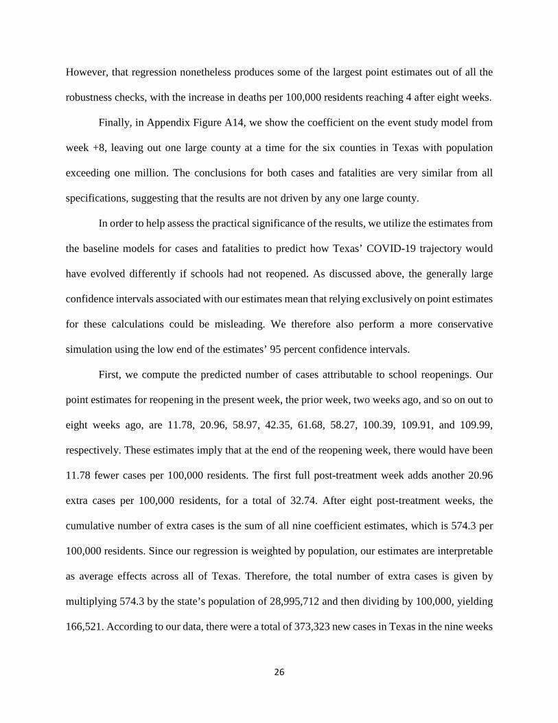
Finally, in Appendix Figure A14, we show the coefficient on the event study model from
week +8, leaving out one large county at a time for the six counties in Texas with population
exceeding one million. The conclusions for both cases and fatalities are very similar from all
specifications, suggesting that the results are not driven by any one large county.
In order to help assess the practical significance of the results, we utilize the estimates from
the baseline models for cases and fatalities to predict how Texas’ COVID-19 trajectory would
have evolved differently if schools had not reopened. As discussed above, the generally large
confidence intervals associated with our estimates mean that relying exclusively on point estimates
for these calculations could be misleading. We therefore also perform a more conservative
simulation using the low end of the estimates’ 95 percent confidence intervals.
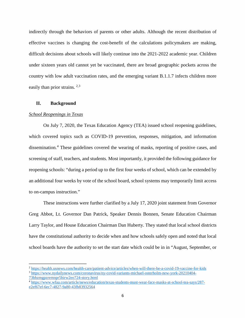
First, we compute the predicted number of cases attributable to school reopenings. Our
point estimates for reopening in the present week, the prior week, two weeks ago, and so on out to
eight weeks ago, are 11.78, 20.96, 58.97, 42.35, 61.68, 58.27, 100.39, 109.91, and 109.99,
respectively. These estimates imply that at the end of the reopening week, there would have been
11.78 fewer cases per 100,000 residents. The first full post-treatment week adds another 20.96
extra cases per 100,000 residents, for a total of 32.74. After eight post-treatment weeks, the
cumulative number of extra cases is the sum of all nine coefficient estimates, which is 574.3 per
100,000 residents. Since our regression is weighted by population, our estimates are interpretable
as average effects across all of Texas. Therefore, the total number of extra cases is given by
multiplying 574.3 by the state’s population of 28,995,712 and then dividing by 100,000, yielding
166,521. According to our data, there were a total of 373,323 new cases in Texas in the nine weeks

27
included in our post-treatment window (including the treatment week itself). Therefore, the point
estimates imply that Texas’ caseload would have been almost 45 percent lower during that time
had schools not reopened.
As stated above, we caution against a literal interpretation of that number given the
relatively wide confidence intervals associated with our estimates. A safer interpretation can be
obtained by instead using the low end of the 95 percent confidence interval to determine the
minimum number of cases attributable to school reopenings implied by our results. The low end
of the 95 percent confidence intervals associated with the variables for the treatment week and
each of the eight post-treatment weeks are -2.88, -13.67, 9.39, -2.72, 12.74, 5.30, 51.12, 55.5, and
33.37, for a total of 148.15. Scaling up to the population of Texas yields a minimum of 42,956
cases attributable to school reopenings in the nine subsequent weeks, or 11.5 percent of the state’s
total caseload during that time.
The same process can be used to compute the number of fatalities attributable to school
reopenings. The baseline regression’s point estimates for the treatment week and eight post-
treatment week variables are 0.35, 0.61, 0.91, 1.3, 1.21, 1.51, 1.98, and 2.36, for a total of 2.36
deaths per 100,000 residents, or 3,021 across the state of Texas. The corresponding low ends of
the 95 percent confidence intervals are -0.05, 0.18, 0.35, 0.54, 0.44, 0.61, 0.83, and 1,07, which
sum to 1.07 fatalities per 100,000 residents, or 818 total across the state. During the time frame,
there were 4,796 COVID-19 fatalities in Texas, so the point estimates imply that 63 percent of
them were due to school reopenings, while the confidence intervals imply that at least 17 percent
of them were.
In sum, even under conservative assumptions, reopening schools had a meaningful impact
on both COVID-19 cases and associated fatalities in Texas. It is noteworthy that the percentage

28
impacts on both outcomes are roughly similar. Ex ante, one might have expected the increase in
deaths to be much smaller proportionally than the rise in cases. COVID-19 mortality rates are
nearly zero for children and are much smaller for the working-age adults who comprise the
majority of school teachers and staff than they are for elderly or vulnerable adults. Our results
therefore suggest that school-reopening-induced COVID-19 spread is reaching more vulnerable
segments of the population. One possible explanation is secondary spread, where infected kids or
employees spread the virus to older, more at-risk individuals. However, this explanation appears
incomplete, as it would imply a several-week lag between new cases and new deaths, which we
do not observe in the data. Another possibility is spillover effects, where schools opening signals
to the community that it is safe to return to normal activities including returning to in-person work,
leading to spread across all segments of the population that may not originate in schools. Such
indirect effects could also help to explain the large effect sizes. The next section explores the
possibility of spillovers more directly.
VI. Spillover Effects on Mobility
We next use SafeGraph data to explore whether changes in mobility patterns among adults
may help to explain the large sizes of the effects of school reopenings on COVID-19 cases and
deaths. Our baseline regression is again an event-study model given by (1), with the reopening
variable defined by the largest potential week-to-week increase in in-person enrollment. However,
we make three small changes in order to customize the approach for mobility outcomes. First, in
contrast to the lags inherent in COVID-19 cases and deaths, effects on mobility can emerge
immediately, and it is not obvious that they will evolve over time. Therefore, we shorten the
window on each side of treatment to six weeks rather than eight, which prevents any counties’
post-treatment windows from extending into the holiday break. The analysis therefore uses 13
29
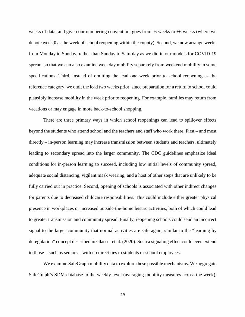
weeks of data, and given our numbering convention, goes from -6 weeks to +6 weeks (where we
denote week 0 as the week of school reopening within the county). Second, we now arrange weeks
from Monday to Sunday, rather than Sunday to Saturday as we did in our models for COVID-19
spread, so that we can also examine weekday mobility separately from weekend mobility in some
specifications. Third, instead of omitting the lead one week prior to school reopening as the
reference category, we omit the lead two weeks prior, since preparation for a return to school could
plausibly increase mobility in the week prior to reopening. For example, families may return from
vacations or may engage in more back-to-school shopping.
There are three primary ways in which school reopenings can lead to spillover effects
beyond the students who attend school and the teachers and staff who work there. First – and most
directly – in-person learning may increase transmission between students and teachers, ultimately
leading to secondary spread into the larger community. The CDC guidelines emphasize ideal
conditions for in-person learning to succeed, including low initial levels of community spread,
adequate social distancing, vigilant mask wearing, and a host of other steps that are unlikely to be
fully carried out in practice. Second, opening of schools is associated with other indirect changes
for parents due to decreased childcare responsibilities. This could include either greater physical
presence in workplaces or increased outside-the-home leisure activities, both of which could lead
to greater transmission and community spread. Finally, reopening schools could send an incorrect
signal to the larger community that normal activities are safe again, similar to the “learning by
deregulation” concept described in Glaeser et al. (2020). Such a signaling effect could even extend
to those – such as seniors – with no direct ties to students or school employees.
We examine SafeGraph mobility data to explore these possible mechanisms. We aggregate
SafeGraph’s SDM database to the weekly level (averaging mobility measures across the week),

30
where our unit of observation is a CBG, which we will refer to as a “neighborhood.” After a
number of screens to the SDM data (discussed in the data section earlier), we examine 14,580
neighborhoods from 252 of the 254 Texas counties. Our four mobility measures, following
SafeGraph’s SDM conventions, are percentage of devices completely at home, percent part-time
work, percent full-time work, and median minutes outside of the dwelling; SafeGraph’s
convention is to define part-time (full-time) “work” as spending 3-6 hours (6 or more hours) at
one location other than home between 8 am and 6 pm local time.31
Using these SafeGraph definitions, in the weeks prior to reopening, approximately 28
percent of devices were completely home on a given day, and nearly 8 percent were engaged in
part-time work and 4 percent in full-time work on a daily basis. In addition, the median time spent
outside of the home on a given day was 108 minutes.
The event-study specifications provide evidence of increased mobility. As illustrated in
Figure 5, only one out of sixteen pre-trend coefficients from six to three weeks prior to reopening
are significantly different from the lead term two weeks prior to reopening. There is some evidence
of anticipation effects in the week immediately prior to reopening with significant increases in
work behavior. Starting in the week of reopening, and essentially thereafter, there is strong
evidence of increased mobility. In the first week of school reopening (week 0), there is a reduction
in staying completely home of 0.7 percentage points, increases in part-time and full-time work of
0.4 percentage points, and increases in time outside the home of more than 8 minutes. These results
persist – and all grow substantially larger – in the subsequent weeks. For example, in week 6, the
mobility results are two to three times as large. and time outside the home increases by 20 minutes.
By the end of the period, relative to the baseline prior to reopening, these are decreases of 5 percent
31 https://docs.safegraph.com/docs/social-distancing-metrics

31
in completely at home per day, increases of 12 percent and 21 percent in part and full time work,
and increases of 18 percent in time outside the home.
Next, we examine these mobility patterns in another way. Schools operate during
weekdays, not weekends. Thus, increases in daily mobility induced by school openings (e.g.,
children at school, parental labor supply) should be more prominent on weekdays. When we run
the same event study models on weekdays only in Figure 6a, the mobility effects are much
stronger, suggesting these mechanisms are operating as expected. To illustrate, in the full-week
model, recall that there was a reduction in staying completely home of 0.7 percentage points in
week 0; when focused on weekdays, there is now a 1.1 percentage point reduction. In the full week
model, time outside the home increased by more than 8 minutes in week 0; when focused on
weekdays, it is now nearly 13 minutes. By week 6, time outside the home increases by 30 minutes
per day, considerably higher than the 20 minutes in the full week model. Relative to the pre-
treatment weekday mean of 116 minutes, this is an increase of 26 percent. When focusing on the
weekend in Figure 6b, we generally find modest reductions in mobility, which may represent an
overall reallocation of activities as the school year begins. For example, time outside the home
falls by between 2 to 5 minutes per day in the weeks after reopening, although many of the
coefficients are insignificant. The overall net effect – as represented by the full week – is clearly
higher mobility.
One key benefit of the SDM database is the level of granularity. The typical neighborhood
in our sample has a population of approximately 1,500 people, and was merged to demographic
data from ACS summary files for 2018 (which aggregates microdata from 2014-2018).
Importantly, these neighborhood summary files contain detailed information on the age
distribution. From this, we characterize neighborhoods in two different ways: whether they have

32
significant numbers of school-age children (fraction of population aged 5 to 17) and whether they
have significant numbers of elderly (fraction of population aged 65 and over). We re-estimate our
models, restricting to neighborhoods in the top quintile of school-age children (neighborhoods
where, on average, approximately 25 percent of the population is comprised of school-aged
children). We also re-estimate models for the top quintile of neighborhoods with elderly (where,
on average, nearly 18 percent of the population are senior citizens). By focusing on neighborhoods
with many children and parents, we expect increases in mobility due to both the resumption of
school and any signaling effects. In contrast, in neighborhoods with large numbers of elderly, the
effects of reopening schools and increased physical work presence should be diminished, although
the general signal that normal activities are safe could still apply.
The overall patterns in the event-study are somewhat stronger for the top quintile of
neighborhoods with school-age children; as illustrated in Figure 7a, the median time away from
home at 6 weeks after opening is nearly 27 minutes, compared with 20 minutes in the full sample.
The pre-trends for all mobility measures show little change in mobility until school reopening, and
then a highly significant and sizable increase thereafter. In contrast, the overall results are more
muted in the elderly sample in Figure 7b. For example, median time away from home shows no
significant increase after school reopenings, and the magnitude is substantively smaller; at 6 weeks
post, time away insignificantly increases by 7 minutes. There is an increase in “full-time work”
(recall, SafeGraph defines this based on extended stays outside the home, not whether the person
is actually at work), yet the magnitudes are again considerably smaller than in neighborhoods with
many children. Put differently, when focused on a sample that should largely be unaffected from
reopenings or increased physical work presence, we see only limited evidence of mobility
consistent with a signal of returning to normal. The results from this granular analysis would then

33
suggest mobility-induced increases from opening schools and potential spillovers onto parental
behavior, especially labor supply.
Finally, we re-examine our main mobility results with a series of robustness checks that
largely mirror the results on COVID-19 in Appendix Figures A15 through A22. Appendix Figure
A15 modifies the event-study specification by additionally including county-specific time trends.
All of the substantive findings remain. For example, 6 weeks after opening, median time away
from home is 20 minutes, virtually identical to the main specification. In Appendix Figure A16,
the specification is amended to include weekly controls for average temperature, precipitation, and
snowfall, factors that have been shown to affect mobility (Kapoor et al., 2020; Wilson, 2020). In
all instances, none of the pre-trends from six to three weeks prior to reopening are different from
the omitted lead of two week; additionally, the results on mobility virtually mirror the baseline,
full-week results. Next, in Appendix Figure A17, we shorten the window to 4 weeks on either side
of the school reopening. The same general patterns emerge as in the baseline specification. For
example, in this specification, time away from home 4 weeks after reopening significantly
increases by more than 15 minutes; in the base specification, it was 17 minutes. In Appendix
Figures A18-A20, we modify the parameterization of school reopenings, by considering a county
to be open if 50 percent, 20 percent, or any students had in-person learning offered to them. As the
figures make clear, how one characterizes school reopening at the county level matters for the
interpretation of the mobility results. In one case (50 percent threshold), there are essentially no
mobility effects (and the pre-trends are generally insignificant). In other cases (20 percent
threshold or greater than 0 percent), the pre-trends for many of the mobility measures are
significant, yet there are no mobility impacts after the “opening”. Next, in Appendix Figure A21,
we modify the baseline specification by including an interaction of Trump’s 2016 county vote

34
share with week fixed effects. The same general patterns remain as in the baseline, but some of
the estimated impacts are smaller and insignificant. Thus, evolving attitudes of Trump voters
appears to be related both to school openings and increased mobility. Finally, in Appendix Figure
A22, we display the coefficient from week +6 from event study models that leave out the six largest
Texas counties, each with population exceeding one million, one at a time. The estimated impacts
on mobility are quite similar to the exercise, suggesting that none of the large counties are driving
our results.
Collectively, these results suggest that reopening schools leads to important spillover
effects on adult mobility that may help to explain the large effect sizes for the COVID-19
outcomes. The evidence is consistent with parents going physically back to work and perhaps also
increasing outside-the-home leisure activities. These effects could be due to lessened child care
responsibilities, signaling about the safety of returning to normal activities, or a combination of
both. In contrast, the evidence is not as strong for neighborhoods with large numbers of elderly
residents or for the general population on weekends, which may suggest that the time-use
mechanism is relatively more important than general signaling.
VII. Conclusion
In this study, we examine the impact of opening Texas public schools for in-person
instruction in fall 2020 on community spread of COVID-19 as well as fatalities. In the eight weeks
after reopening, we conservatively estimate, based on lower bounds of confidence intervals, that
there would have been at least 43,000 fewer COVID-19 cases and at least 800 fewer fatalities.
These results hold across a variety of specifications and robustness checks. These results could be
explained both by the direct effect of spread within the schools and the indirect effects of increased
mobility within the community as our analysis of cellphone data suggests that six weeks after

35
reopening, the median time spent outside of the home increased by 26 percent on weekdays. This
suggests that decision makers need to think strategically about how to encourage behavior to
mitigate spread of COVID-19 not only within schools, but within the community at large.
On the surface, our empirical findings diverge with several popular narratives that have
emerged about school openings. Some studies – including a prominent CDC study from Wisconsin
– rely on contract tracing efforts to quantify impacts of school reopening. The imperfections of
run-of-the-mill contact tracing efforts – including the inability to follow asymptomatic cases or
lack of cooperation in finding all close contacts – suggests estimates of in-school spread may be a
lower bound. Importantly, this approach does not account for inevitable, indirect behaviors – such
as greater parental mobility including increased physical presence in the workplace – which also
may contribute to community spread. Although other recent research teams (Tulane, CALDER)
take methodological approaches closer to our approach and find overall more modest effects on
COVID-19 spread, it is important to emphasize that the initial conditions in Texas were more ripe
for community spread and schools opened more widely, more quickly, and generally, close to full
capacity.
Although it is beyond the scope of our study to provide a cost-benefit analysis of school
reopenings, our quantitative findings contribute a key input into such an analysis. Recent work by
Kniesner and Sullivan (2020) estimate non-fatal economic losses of about $46,000 per case, and
Department of Transportation apply an $11 million loss per fatality. Such health- and productivity-
related losses from COVID-19 must be weighed against learning losses for children, as well as
other ancillary effects related to child mental health and abuse and these losses could be substantial
but will only become clear over time. Distributional considerations are also important, as benefits

36
of school closures accrue disproportionately among older individuals, whereas the costs are largely
borne by children.
Obviously, as vaccinations expand, the cost-benefit calculations of opening schools
changes. As of early April 2021, approximately 33 percent of adults aged 18 and older have been
at least partially vaccinated, and the percentage is considerably higher among the most
vulnerable.32 To the extent that the spread of new mutations of the virus are mitigated by vaccines,
almost all policies that restrict mobility – including school closures – will eventually be
unnecessary. Nonetheless, there continue to be pockets of high spread of COVID-19. Furthermore,
among various groups, there is widespread vaccine hesitancy and mistrust of the medical system.
For instance, in a survey conducted in February 2021, among white evangelical adults, 45 percent
stated they would “definitely not” or “probably not” get the COVID-19 vaccine.33 In addition,
vaccination rates are stubbornly low in both the African-American and Hispanic communities34,
potentially due to historic mistrust of medical providers (Alsan and Wanamaker, 2018). As of April
2021, Texas lags the national average in both partial and full vaccinations, as do many of the states
in the South.35 Collectively, this suggests that there will be significant pockets of communities
where lack of restrictions – including the opening of schools – may still lead to considerable
community spread moving forward. Additionally, the B.1.1.7 variant that is gradually becoming
the dominant strain in the U.S. infects children more easily than prior strains, and children under
sixteen years old cannot yet be vaccinated. 36,37
32 https://www.nytimes.com/interactive/2020/us/covid-19-vaccine-doses.html 33 https://www.pewresearch.org/fact-tank/2021/03/23/10-facts-about-americans-and-coronavirus-vaccines/ft_21-03-18_vaccinefacts/ 34 https://www.kff.org/coronavirus-covid-19/issue-brief/latest-data-on-covid-19-vaccinations-race-ethnicity/ 35 https://www.nytimes.com/interactive/2020/us/covid-19-vaccine-doses.html 36 https://www.nydailynews.com/coronavirus/ny-covid-variants-michael-osterholm-new-york-20210404-73bhzmgpzremnpr5hirw2eo724-story.html 37 https://health.usnews.com/health-care/patient-advice/articles/when-will-there-be-a-covid-19-vaccine-for-kids

37
For these reasons, debate about school openings and mitigation strategies will therefore
likely continue to persist into the 2021-2022 school year, and our results provide important
information that can help inform that debate. In particular, the CDC guidelines say that schools
can reopen if community spread is low and considerable precautions are taken. Our study is not
necessarily at odds with that guidance; instead, it simply shows that school reopenings are not
always safe if those conditions are not met.
REFERENCES Allcott, H., Boxell, L., Conway, J., Gentzkow, M., Thaler, M., & Yang, D. (2020). “Polarization
and public health: Partisan differences in social distancing during the coronavirus pandemic.” Journal of Public Economics 191:104254, doi:10.1016/j.jpubeco.2020.104254
Alsan, M. & Wanamaker, M. (2018). “Tuskegee and the Health of Black Men.” The Quarterly
Journal of Economics 133(1): 407–455, doi:10.1093/qje/qjx029 Andersen, M., Bryan, S., & Slusky, D. (2020). “COVID-19 Surgical Abortion Restriction Did
Not Reduce Visits to Abortion Clinics.” National Bureau of Economic Research Working Paper Series, No. 28058. doi:10.3386/w28058
Auger K.A., Shah S.S., Richardson T., et al. (2020) “Association Between Statewide School
Closure and COVID-19 Incidence and Mortality in the US.” JAMA 324(9):859–870. doi:10.1001/jama.2020.14348.
Bailey, M., Johnston, D.M., Koenen, M., Kuchler, T., Russel, D., & Stroebel, J. (2020). “Social
Networks Shape Beliefs and Behavior: Evidence from Social Distancing During the COVID-19 Pandemic.” National Bureau of Economic Research Working Paper Series, No. 28234. doi:10.3386/w28234
Baker, A.C., D. Larcker, and C.C.Y. Wang (2021). “How Much Should We Trust Staggered
Difference-in-Differences Estimates.” EGCI Finance Working Paper 736/2021. Bullinger, L.R., Carr, J.B., & Packham, A. (Forthcoming). “COVID-19 and Crime: Effects of
Stay-at-Home Orders on Domestic Violence.” American Journal of Health Economics, doi:10.1086/713787

38
Callaway, B. & Sant’Anna, P.H.C. (Forthcoming). “Difference-in-Differences With Multiple Time Periods.” Journal of Econometrics. doi:10.1016/j.jeconom.2020.12.001
Cengiz, D., A. Dube, A. Lindner, and B. Zipperer (2019). “The Effect of Minimum Wages on
Low-Wage Jobs.” The Quarterly Journal of Economics 134 (3), 1405-1454. Council of Economic Advisers. (2020). Reopening Schools Is Key to Unlocking the Full
Potential of America’s Children. The White House. https://www.whitehouse.gov/articles/reopening-schools-key-unlocking-full-potential-americaschildren/
Cotti, C., Engelhardt, B., Foster, J., Nesson, E., & Niekamp, P. (Forthcoming). “The relationship
between in-person voting and COVID-19: Evidence from the Wisconsin primary.” Contemporary Economic Policy, doi:10.1111/coep.12519
Courtemanche, C., Garuccio, J., Le, A., Pinkston, J., & Yelowitz, A. (2020). “Strong Social
Distancing Measures in the United States Reduced the COVID-19 Growth Rate.” Health Affairs 39(7): 1237–1246. doi:10.1377/hlthaff.2020.00608
Cronin, C.J., & Evans, W.N. (2020). “Private Precaution and Public Restrictions: What Drives
Social Distancing and Industry Foot Traffic in the COVID-19 Era?” National Bureau of Economic Research Working Paper Series, No. 27531. doi:10.3386/w27531
Cunningham, S. (2021). Causal Inference: The Mixtape. New Haven, CT: Yale University Press. Dave, D., Friedson, A. I., Matsuzawa, K., & Sabia, J. J. (2021). “When Do Shelter-In-Place
Orders Fight COVID-19 Best? Policy Heterogeneity Across states and Adoption Time.” Economic Inquiry 59(1): 29–52. doi:10.1111/ecin.12944
Dave, D.M., Friedson, A.I., Matsuzawa, K., Sabia, J.J., & Safford, S. (2020a). “Black Lives
Matter Protests and Risk Avoidance: The Case of Civil Unrest During a Pandemic.” National Bureau of Economic Research Working Paper Series, No. 27408. doi:10.3386/w27408
Dave, D., McNichols, D., & Sabia, J.J. (2020b). “The contagion externality of a superspreading
event: The Sturgis Motorcycle Rally and COVID‐19” Southern Economic Journal 87(3): 769–807. doi:10.1002/soej.12475
de Chaisemartin, C. & D'Haultfœuille, X. (2020). “Two-Way Fixed Effects Estimators with
Heterogeneous Treatment Effects.” American Economic Review 110(9): 2964–96. doi:10.1257/aer.20181169

39
Doyle T, Kendrick K, Troelstrup T, et al. (2021). “COVID-19 in Primary and Secondary School Settings During the First Semester of School Reopening — Florida, August–December 2020.” MMWR Morb Mortal Wkly Rep 2021;70:437–441. doi:10.15585/mmwr.mm7012e2
Dub, T., Erra, E., Hagberg, L., Sarvikivi, E., Virta, C., Jarvinen, A., Osterlund, P., Ikonen, N.,
Haveri, A., Melin, M., Lukkarinen, T. J., & Nohynek, H. (2020). “Transmission of SARS-CoV-2 following exposure in school settings: Experience from two Helsinki area exposure incidents.” MedRxiv, 2020.07.20.20156018. doi:10.1101/2020.07.20.20156018
Falk, A., Benda, A., Falk, P., Steffen, S., Wallace, Z., & Høeg, T.B. (2021) “COVID-19 Cases
and Transmission in 17 K–12 Schools — Wood County, Wisconsin, August 31–November 29, 2020.” MMWR Morb Mortal Wkly Rep 2021;70:136–140. doi:10.15585/mmwr.mm7004e3
Flaxman, S., Mishra, S., Gandy, A. et al. (2020). “Estimating the effects of non-pharmaceutical
interventions on COVID-19 in Europe.” Nature 584:257–261. doi:10.1038/s41586-020-2405-7
Fontanet, A., Grant, R., Tondeur, L., Madec, Y., Grzelak, L., Cailleau, I., Ungeheuer, M.N.,
Renaudat, C., Pellerin, S. F., Kuhmel, L., et al. (2020). “SARS-CoV-2 infection in primary schools in northern France: A retrospective cohort study in an area of high transmission.” MedRxiv. doi:10.1101/2020.06.25.20140178
Friedson, A.I., McNichols, D., Sabia, J.J., & Dave, D. (Forthcoming). “Shelter-In-Place Orders
and Public Health: Evidence From California During the COVID-19 Pandemic.” Journal of Policy Analysis and Management, doi:10.1002/pam.22267
Glaeser, E.L., Jin, G.Z., Leyden, B.T., & Luca, M. (2020). “Learning from Deregulation: The
Asymmetric Impact of Lockdown and Reopening on Risky Behavior During COVID-19.” National Bureau of Economic Research Working Paper Series, No. 27650. doi:10.3386/w27650
Goldhaber, D., Imberman, S., Strunk, K, Hopkins, B., Brown, N., Harbatkin, E., & Kilbride, T.
(2021). “To What Extent Does In-Person Schooling Contribute to the Spread of COVID-19? Evidence from Michigan and Washington.” American Institute for Research, working paper 247-2020-2. https://caldercenter.org/sites/default/files/CALDER%20WP%20247-1220-2.pdf
Goodman-Bacon, A. (Forthcoming). “Difference-in-Differences with Variation in Treatment
Timing.” Journal of Econometrics.

40
Green, D.A., Karimirad, A., Simard-Duplain, G., & Siu, H.E. (2020). “COVID and the Economic Importance of In-Person K-12 Schooling,” National Bureau of Economic Research Working Paper Series, No. 28200. doi:10.3386/w28200
Gupta, S., Nguyen, T.D., Rojas, F.L., Raman, S., Lee, B., Bento, A., & Wing, C. (2020).
“Tracking Public and Private Responses to the COVID-19 Epidemic: Evidence from State and Local Government Actions.” National Bureau of Economic Research Working Paper Series, No. 27027. doi:10.3386/w27027
Harris, D., Ziedan, E., & Hassig, S. (2021). “The Effects of School Reopenings on COVID-19
Hospitalization.” National Center for Research on Education Access and Choice. Available at: The-Effects-of-School-Reopenings-on-COVID-19-Hospitalizations-REACH-January-2021.pdf
Hsiang, S., Allen, D., Annan-Phan, S. et al. (2020). “The effect of large-scale anti-contagion
policies on the COVID-19 pandemic.” Nature 584, 262–267. doi:10.1038/s41586-020-2404-8
Honein, M.A., Barrios, L.C., & Brooks, J.T. (2021) “Data and Policy to Guide Opening Schools
Safely to Limit the Spread of SARS-CoV-2 Infection.” JAMA. 325(9):823–824. doi:10.1001/jama.2021.0374
Hurt, S., Ball, A., & Wedell, K. (2020). “Children more at risk for abuse and neglect amid
coronavirus pandemic, experts say.” USA Today, March 21, Accessed on April 14, 2021 at: https://www.usatoday.com/story/news/investigations/2020/03/21/coronavirus-pandemic-could-become-child-abuse-pandemic-experts-warn/2892923001/
Isphording, I.E., Lipfert, M., & Pestel, N. (2020). “School Re-Openings after Summer Breaks in
Germany Did Not Increase SARS-CoV-2 Cases.” IZA Institute of Labor Economics, IZA DP No. 13790. Retrieved from http://ftp.iza.org/dp13790.pdf
Kniesner, T.J., & Sullivan, R. (2020) “The forgotten numbers: A closer look at COVID-19 non-
fatal valuations.” Journal of Risk and Uncertainty 61:155–176. doi:10.1007/s11166-020-09339-0
Kuhfeld, M., Soland, J., Tarasawa, B., Johnson, A., Ruzek, E., & Liu, J. (2020). “Projecting the
potential impacts of COVID-19 school closures on academic achievement.” (EdWorkingPaper: 20-226). Retrieved from Annenberg Institute at Brown University: https://doi.org/10.26300/cdrv-yw05
Kuhfeld, M., & Tarasawa, B. (2020). “The COVID-19 slide: What summer learning loss can tell
us about the potential impact of school closures on student academic achievement.” The Collaborative for Student Growth NWEA White Paper.

41
https://www.nwea.org/research/publication/the-covid-19-slide-what-summer-learning-loss-can-tell-us-about-the-potential-impact-of-school-closures-on-student-academic-achievement/
Ludvigsson, J.F. (2020). “Children are unlikely to be the main drivers of the COVID-19
pandemic – A systematic review.” Acta Paediatrica 109(8):1525–1530. doi:10.1111/apa.15371
Maldonado, J.E., & De Witte K. (2020) “The effect of school closure on standardized student
test outcomes.” Discussion paper series DPS20.17. Belgium: KU Leuven. Milosh, M., Painter, M., Sonin, K., Van Dijcke, D., & Wright, A.L. (2020), “Unmasking
Partisanship: How Polarization Influences Public Responses to Collective Risk”, University of Chicago, Becker Friedman Institute for Economics Working Paper (2020-102)
MIT Election Data and Science Lab, (2018), “County Presidential Election Returns 2000-2016”,
https://doi.org/10.7910/DVN/VOQCHQ, Harvard Dataverse, V6, UNF:6:ZZe1xuZ5H2l4NUiSRcRf8Q== [fileUNF]
Schmidt, S. & Natanson H. (2020). “With kids stuck at home, ER doctors see more severe cases
of child abuse.” Washington Post. Accessed on February 20, 2021 at: https://www.washingtonpost.com/education/2020/04/30/child-abuse-reports-coronavirus/
Simmons-Duffin, S.S. (2020). “14 States Make Contact Tracing Data Public. Here's What
They're Learning.” Available at https://www.npr.org/sections/health-shots/2020/08/14/902271822/13-states-make-contact-tracing-data-public-heres-what-they-re-learning
Simonov, A., Sacher, S. K., Dubé, J.P.H., & Biswas, S. (2020). “The Persuasive Effect of Fox
News: Non-Compliance with Social Distancing During the Covid-19 Pandemic.” National Bureau of Economic Research Working Paper Series, No. 27237. doi:10.3386/w27237
Valant, J. (2020). “School reopening plans linked to politics rather than public health.” Brown
Center Chalkboard, Brookings Institution. Accessed at https://www.brookings.edu/blog/brown-center-chalkboard/2020/07/29/school-reopening-plans-linked-to-politics-rather-than-public-health/

42
Table 1: Means and Standard Deviations of Outcome Variables (1) (2) COVID Outcomes Pre-reopening Post-reopening New cases per 100,000 residents 147.73 139.74
(121.37) (171.99) New deaths per 100,000 residents 3.51 1.80
(5.45) (3.72)
Observations 2,024 2,277 Mobility Outcomes Pre-reopening Post-reopening Time Completely Home (%) 28.21 26.62
(5.94) (5.72) Part-time Work (%) 7.84 9.00
(2.25) (2.65) Full-time Work (%) 3.98 4.93
(1.35) (1.69) Median non-home dwelling time (minutes) 107.76 128.25
(56.42) (62.10) Observations 87,480 102,060 Notes: Standard deviations are in parentheses. The COVID outcomes utilize public county-by-week-level data, while the mobility outcomes are from census-block-group-by-week-level data from SafeGraph. Observations are weighted by county (census-block-group) population for the COVID (mobility) variables. The pre-reopening period refers to the eight (six) weeks prior to school reopenings for the COVID (mobility) variables. The post-reopening period refers to the reopening week along with the eight (six) weeks following reopening for the COVID (mobility) variables.

43
Table 2: Predictors of Reopening Week
Coefficient estimate
(standard error) Standardized 2016 percent of votes for President Trump -1.18***
(0.30) Standardized percent Hispanic -0.19
(0.15) Standardized percent Black -0.15
(0.12) Standardized population 0.18
(0.16) Standardized percent who stayed at home for full day 0.07
(0.15) Standardized new weekly cases per 100,000 0.32***
(0.12) Constant 17.06***
(0.19) Observations 253 Notes: * p<0.1, ** p<0.05, *** p<0.01. Results are from a cross-sectional county-level linear regression with week number of reopening (ranging from 14 to 28, with 1 indicating the week of May 3) as the outcome variable. The stay-at-home and new cases variables are pooled averages across the four weeks prior to the earliest school reopening (week numbers 10 through 13).

44
Figure 1: Relative Start Date of School District Start Date in 2020-21 School Year Relative to the 2019-20 School Year
Note: In some cases, we do not have the 2019-20 start date for school districts. In these cases, we substitute a prior start date for any year we could find a record.

45
Figure 2. Weekly COVID-19 cases per 100,000 residents in Texas, Washington, Michigan, and the U.S.

46
Figure 3: Event-Study Regression Results for Effect of Reopening Schools on COVID-19 Cases per 100,000 Residents
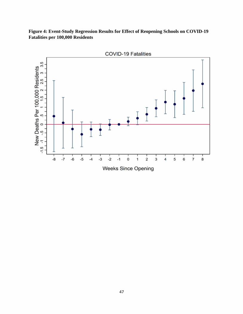
47
Figure 4: Event-Study Regression Results for Effect of Reopening Schools on COVID-19 Fatalities per 100,000 Residents

48
Figure 5: Effects of school reopening on mobility - Baseline model (all CBGs, full-week)
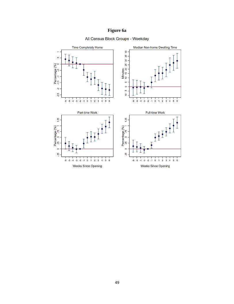
49
Figure 6a
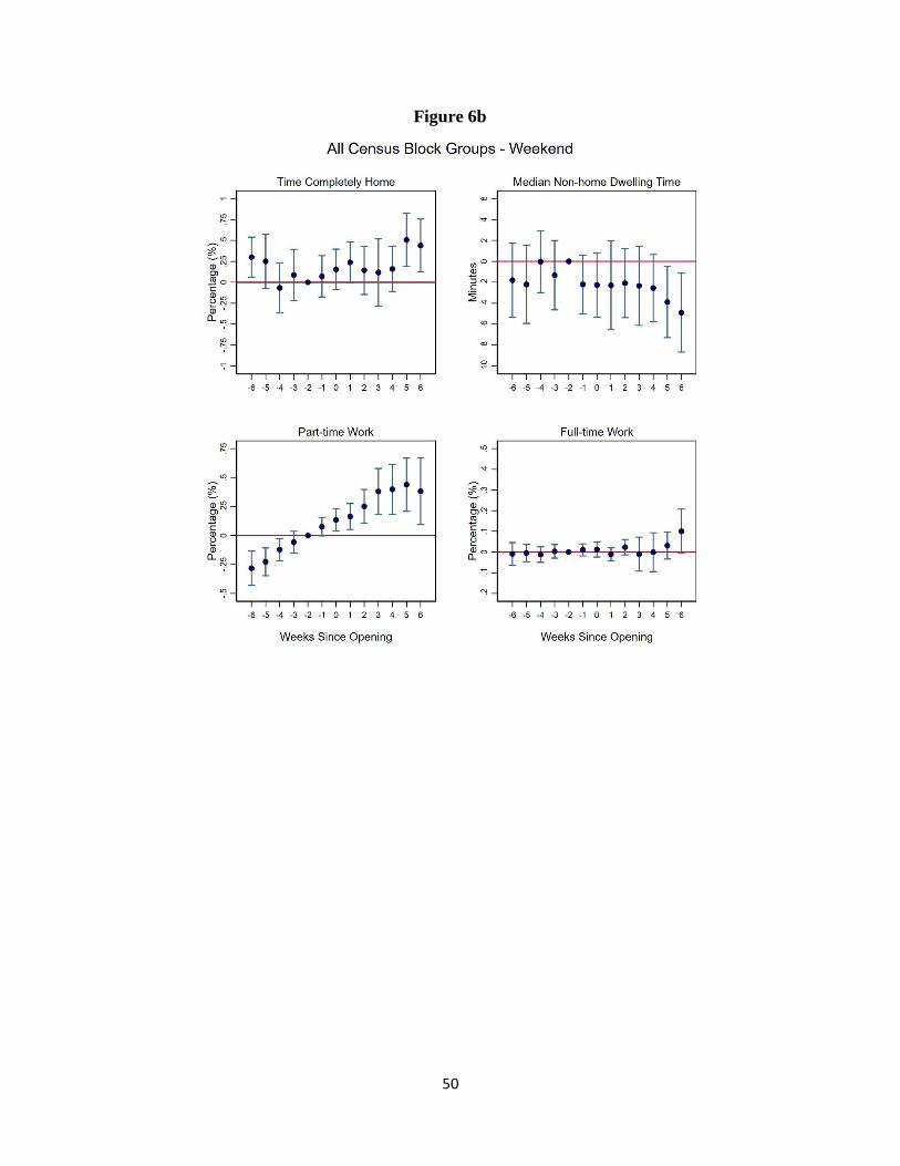
50
Figure 6b

51
Figure 7a

52
Figure 7b

53
Appendix Figures (online only)
Appendix Figure A1. Robustness checks: (a) Control for college reopenings; (b) Control for county-specific time trends; (c) Control for Trump vote share interacted with week fixed effects.
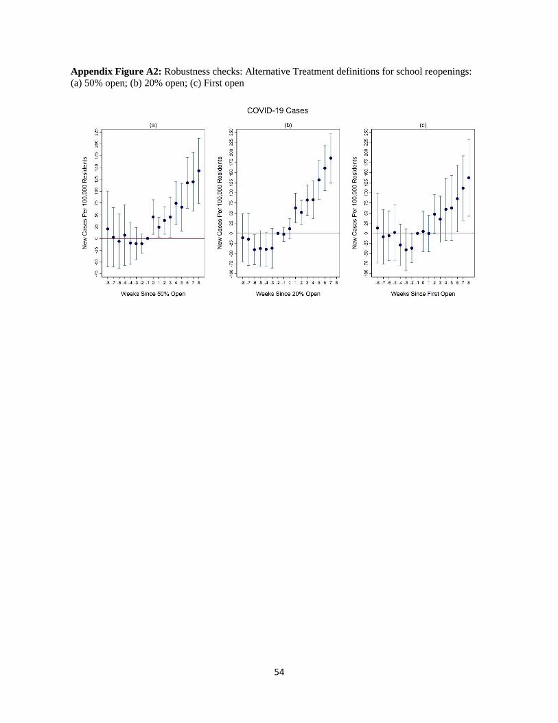
54
Appendix Figure A2: Robustness checks: Alternative Treatment definitions for school reopenings: (a) 50% open; (b) 20% open; (c) First open

55
Appendix Figure A3: Robustness checks: (a) Outcome: cumulative cases exponential growth rate; (b) Outcome: the natural log of new case count.

56
Appendix Figure A4: Robustness checks: (a) Drop testing variables; (b) Control for negative tests.

57
Appendix Figure A5: Robustness checks: (a) 6-week event-study window; (b) 4-week event-study window.

58
Appendix Figure A6: Robustness checks: (a) Drop El Paso County; (b) Drop six counties w/ > 1 mil residents; (c) Unweighted.

59
Appendix Figure A7: Robustness checks:
(a) Stacked regression
(b) Callaway and Sant’ Anna method

60
Appendix Figure A8: Robustness checks: (a) Control for college reopening; (b) Control for county-specific time trends; (c) Control for Trump vote share interacted with week fixed effects.

61
Appendix Figure A9. Alternative Treatment definitions for school reopenings: Robustness checks: (a) 50% open; (b) 20% open; (c) First open.

62
Appendix Figure A10: Robustness checks: (a) Outcome: cumulative cases exponential growth rate; (b) Outcome: the natural log of new case count.

63
Appendix Figure A11: Robustness checks: (a) 6-week event-study window; (b) 4-week event-study window.

64
Appendix Figure A12: Robustness checks: (a) Drop El Paso County; (b) Drop six counties w/ > 1 mil residents; (c) Unweighted.

65
Appendix Figure A13: Robustness checks:
(a) Stacked regression
(b) Callaway and Sant’ Anna method

66
Appendix Figure A14: Specifications leaving-out each of the 6 largest counties in Texas one at a time – COVID-19 outcomes at week +8.

67
Appendix Figure A15 -- Effects of school reopening on mobility - Control for county-specific time trends (all CBGs, full-week sample)

68
Appendix Figure A16 -- Effects of school reopening on mobility - Control for weather variables (all CBGs, full-week sample)

69
Appendix Figure A17 -- Effects of school reopening on mobility - 4-week event-study window (all CBGs, full-week sample)

70
Appendix Figure A18 -- Effects of school reopening on mobility - Treatment defined when 50% of students attend reopened schools (all CBGs, full-week sample)

71
Appendix Figure A19 -- Effects of school reopening on mobility - Treatment defined when 20% of students attend reopened schools (all CBGs, full-week sample)

72
Appendix Figure A20 -- Effects of school reopening on mobility - Treatment defined when first school district reopened (all CBGs, full-week sample)

73
Appendix Figure A21 -- Effects of school reopening on mobility - Control for Trump vote share interacted with week fixed effects (all CBGs, full-week sample)

74
Appendix Figure A22: Specifications leaving-out each of the 6 largest counties in Texas one at a time – mobility outcomes at week +6.