Embed Size (px)
Citation preview
1
Modern ECC signatures
2011 Bernstein–Duif–Lange–
Schwabe–Yang:
Ed25519 signature scheme =
EdDSA using conservative
Curve25519 elliptic curve.
https://ed25519.cr.yp.to
32-byte public keys,
64-byte signatures,
≈2125:8 security level.
Deployed in SSH, Signal,
many more applications:
https://ianix.com/pub
/ed25519-deployment.html

2
Many papers have explored
Curve25519/Ed25519 speed.
e.g. 2015 Chou software:
on Intel Sandy Bridge (2011),
57164 cycles for keygen,
63526 cycles for signature,
205741 cycles for verification,
159128 cycles for ECDH.
Compare to, e.g., 2000 Brown–
Hankerson–Lopez–Menezes:
on Intel Pentium II (1997),
1920000 cycles for ECDH
using NIST P-256 curve.

3
AC : cycles for alg A on CPU C.
Does AC < BD prove that
A is better than B?
3
AC : cycles for alg A on CPU C.
Does AC < BD prove that
A is better than B?
No! Beware change in CPU.
Maybe AC > BC ; AD > BD;
C does more work per cycle than
D, thanks to CPU manufacturer.
Sometimes people measure cost
in seconds instead of cycles.
Then they benefit
from more work per cycle and
from more cycles per second.
4
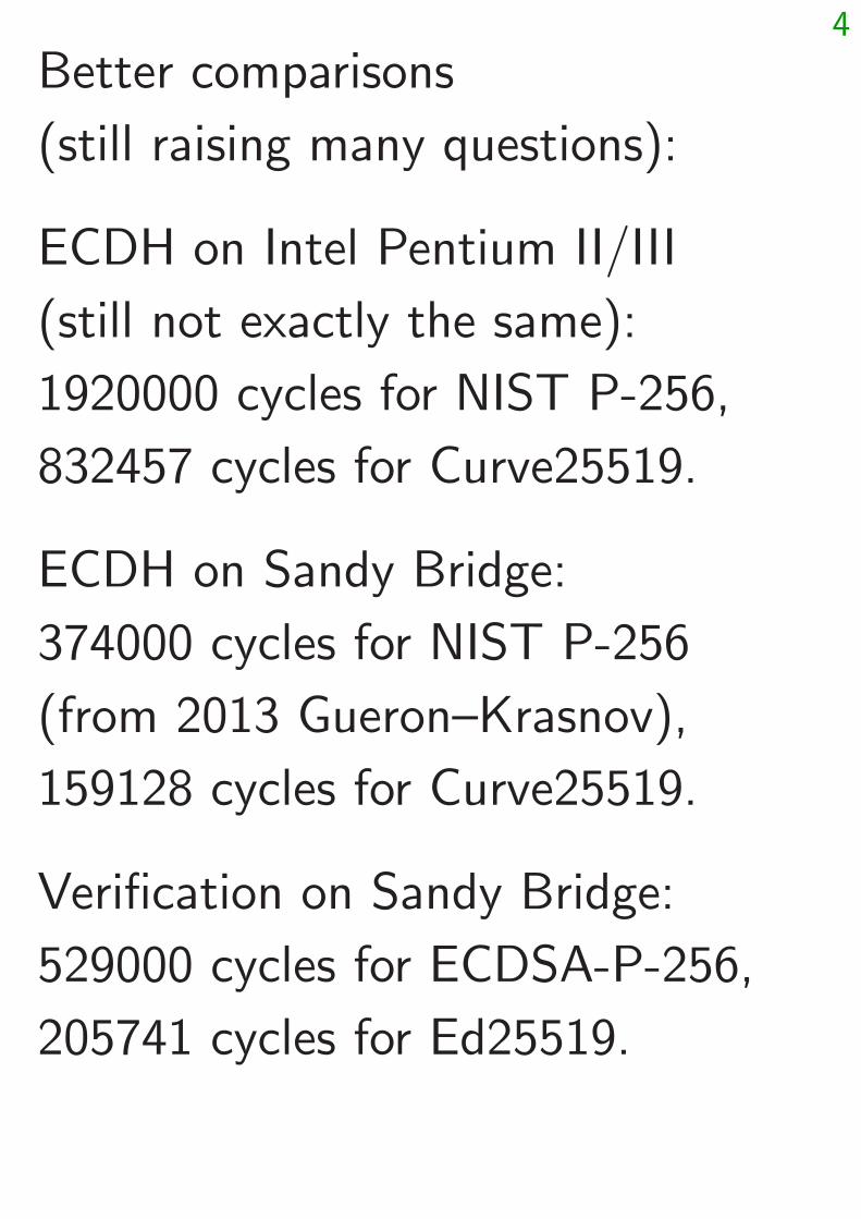
Better comparisons
(still raising many questions):
ECDH on Intel Pentium II/III
(still not exactly the same):
1920000 cycles for NIST P-256,
832457 cycles for Curve25519.
ECDH on Sandy Bridge:
374000 cycles for NIST P-256
(from 2013 Gueron–Krasnov),
159128 cycles for Curve25519.
Verification on Sandy Bridge:
529000 cycles for ECDSA-P-256,
205741 cycles for Ed25519.
5
For each of these operations,
on each of these curves,
on each of these CPUs:
Simplest implementations
are much, much, much slower.
Questions in algorithm design
and software engineering:
How to build the fastest software
on, e.g., an ARM Cortex-A8 for
Ed25519 signature verification?
Answers feed back into crypto
design: e.g., choosing fast curves.
6
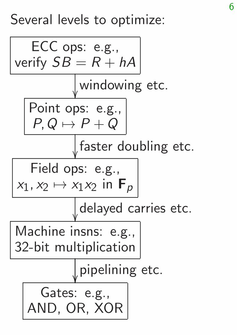
Several levels to optimize:
ECC ops: e.g.,verify SB = R + hA
windowing etc.��
Point ops: e.g.,P;Q 7→ P + Q
faster doubling etc.��
Field ops: e.g.,x1; x2 7→ x1x2 in Fp
delayed carries etc.��
Machine insns: e.g.,32-bit multiplication
��pipelining etc.��
Gates: e.g.,AND, OR, XOR
7
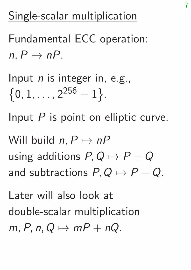
Single-scalar multiplication
Fundamental ECC operation:
n; P 7→ nP .
Input n is integer in, e.g.,˘0; 1; : : : ; 2256 − 1
¯.
Input P is point on elliptic curve.
Will build n; P 7→ nP
using additions P;Q 7→ P + Q
and subtractions P;Q 7→ P − Q.
Later will also look at
double-scalar multiplication
m;P; n;Q 7→ mP + nQ.
8
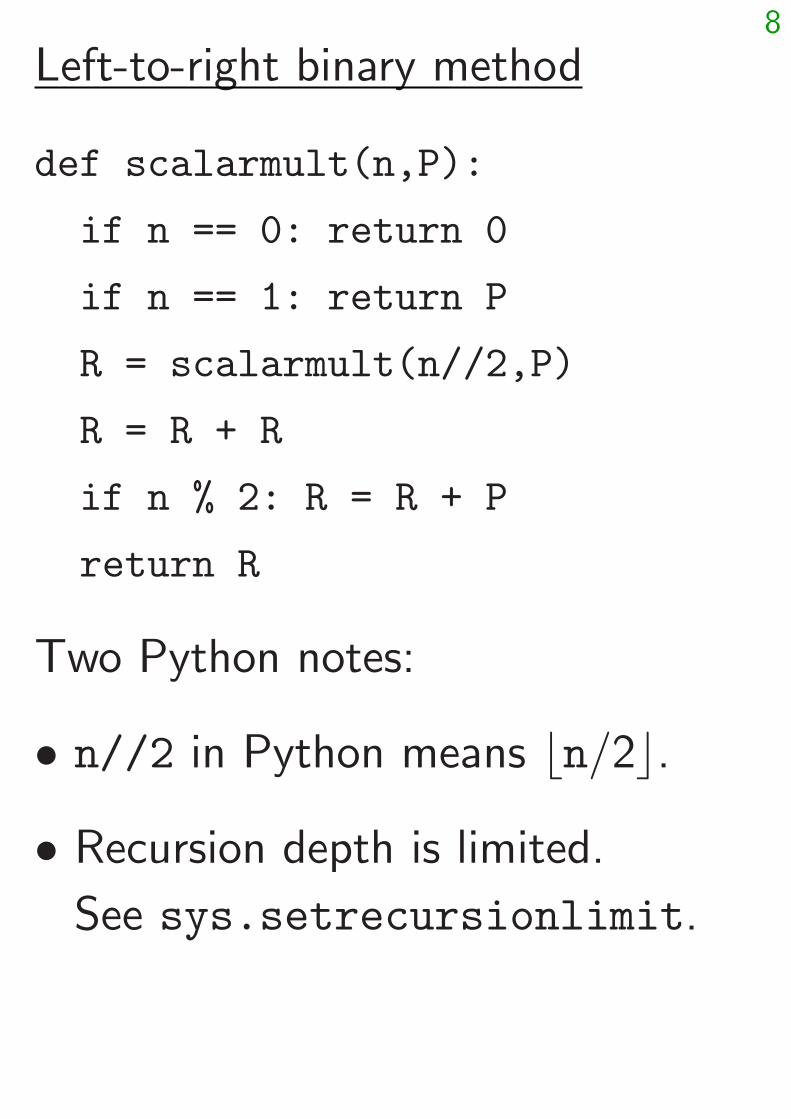
Left-to-right binary method
def scalarmult(n,P):
if n == 0: return 0
if n == 1: return P
R = scalarmult(n//2,P)
R = R + R
if n % 2: R = R + P
return R
Two Python notes:
• n//2 in Python means bn=2c.
• Recursion depth is limited.
See sys.setrecursionlimit.
9
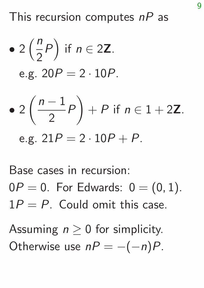
This recursion computes nP as
• 2“n
2P”
if n ∈ 2Z.
e.g. 20P = 2 · 10P .
• 2
„n − 1
2P
«+ P if n ∈ 1 + 2Z.
e.g. 21P = 2 · 10P + P .
Base cases in recursion:
0P = 0. For Edwards: 0 = (0; 1).
1P = P . Could omit this case.
Assuming n ≥ 0 for simplicity.
Otherwise use nP = −(−n)P .
10
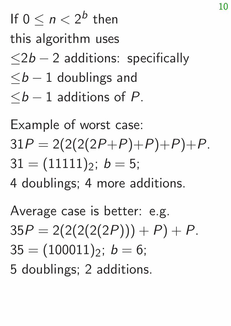
If 0 ≤ n < 2b then
this algorithm uses
≤2b − 2 additions: specifically
≤b − 1 doublings and
≤b − 1 additions of P .
Example of worst case:
31P = 2(2(2(2P+P )+P )+P )+P .
31 = (11111)2; b = 5;
4 doublings; 4 more additions.
Average case is better: e.g.
35P = 2(2(2(2(2P ))) + P ) + P .
35 = (100011)2; b = 6;
5 doublings; 2 additions.
11
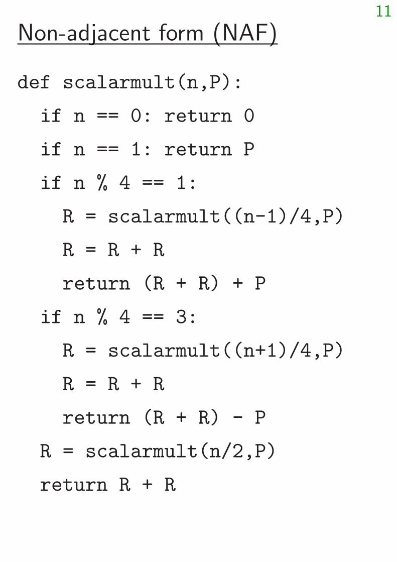
Non-adjacent form (NAF)
def scalarmult(n,P):
if n == 0: return 0
if n == 1: return P
if n % 4 == 1:
R = scalarmult((n-1)/4,P)
R = R + R
return (R + R) + P
if n % 4 == 3:
R = scalarmult((n+1)/4,P)
R = R + R
return (R + R) - P
R = scalarmult(n/2,P)
return R + R
12
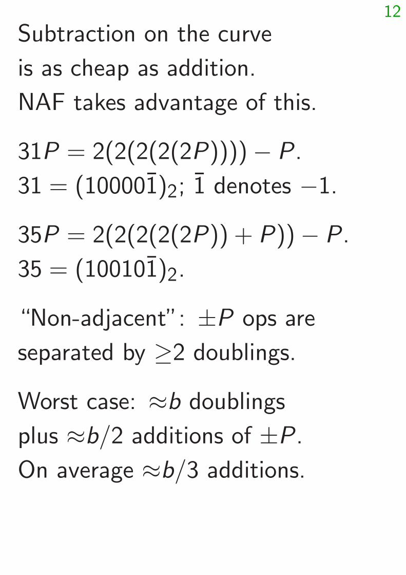
Subtraction on the curve
is as cheap as addition.
NAF takes advantage of this.
31P = 2(2(2(2(2P ))))− P .
31 = (100001)2; 1 denotes −1.
35P = 2(2(2(2(2P )) + P ))− P .
35 = (100101)2.
“Non-adjacent”: ±P ops are
separated by ≥2 doublings.
Worst case: ≈b doublings
plus ≈b=2 additions of ±P .
On average ≈b=3 additions.

13
Width-2 signed sliding windows
def window2(n,P,P3):
if n == 0: return 0
if n == 1: return P
if n == 3: return P3
if n % 8 == 1:
R = window2((n-1)/8,P,P3)
R = R + R
R = R + R
return (R + R) + P
if n % 8 == 3:
R = window2((n-3)/8,P,P3)
R = R + R
R = R + R
return (R + R) + P3

14
if n % 8 == 5:
R = window2((n+3)/8,P,P3)
R = R + R
R = R + R
return (R + R) - P3
if n % 8 == 7:
R = window2((n+1)/8,P,P3)
R = R + R
R = R + R
return (R + R) - P
R = window2(n/2,P,P3)
return R + R
def scalarmult(n,P):
return window2(n,P,P+P+P)
15
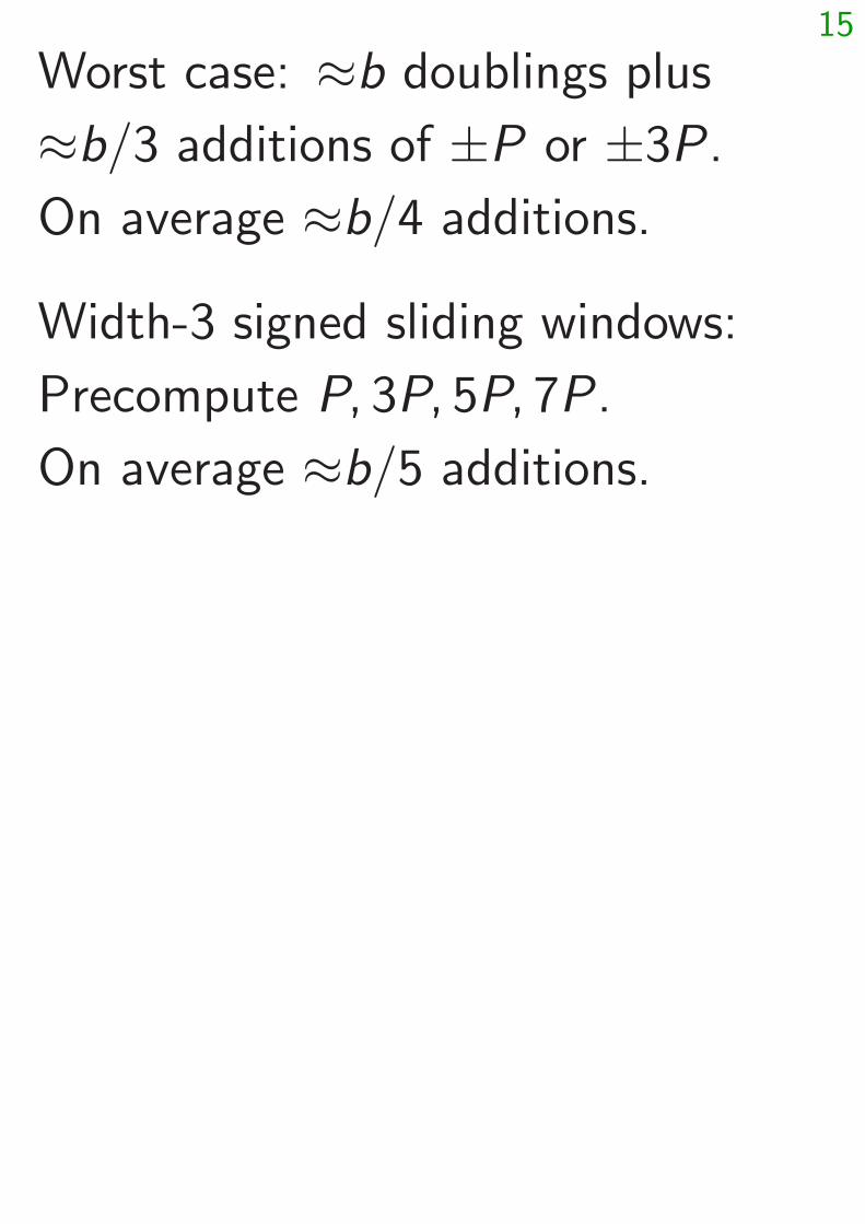
Worst case: ≈b doublings plus
≈b=3 additions of ±P or ±3P .
On average ≈b=4 additions.
15
Worst case: ≈b doublings plus
≈b=3 additions of ±P or ±3P .
On average ≈b=4 additions.
Width-3 signed sliding windows:
Precompute P; 3P; 5P; 7P .
On average ≈b=5 additions.
15
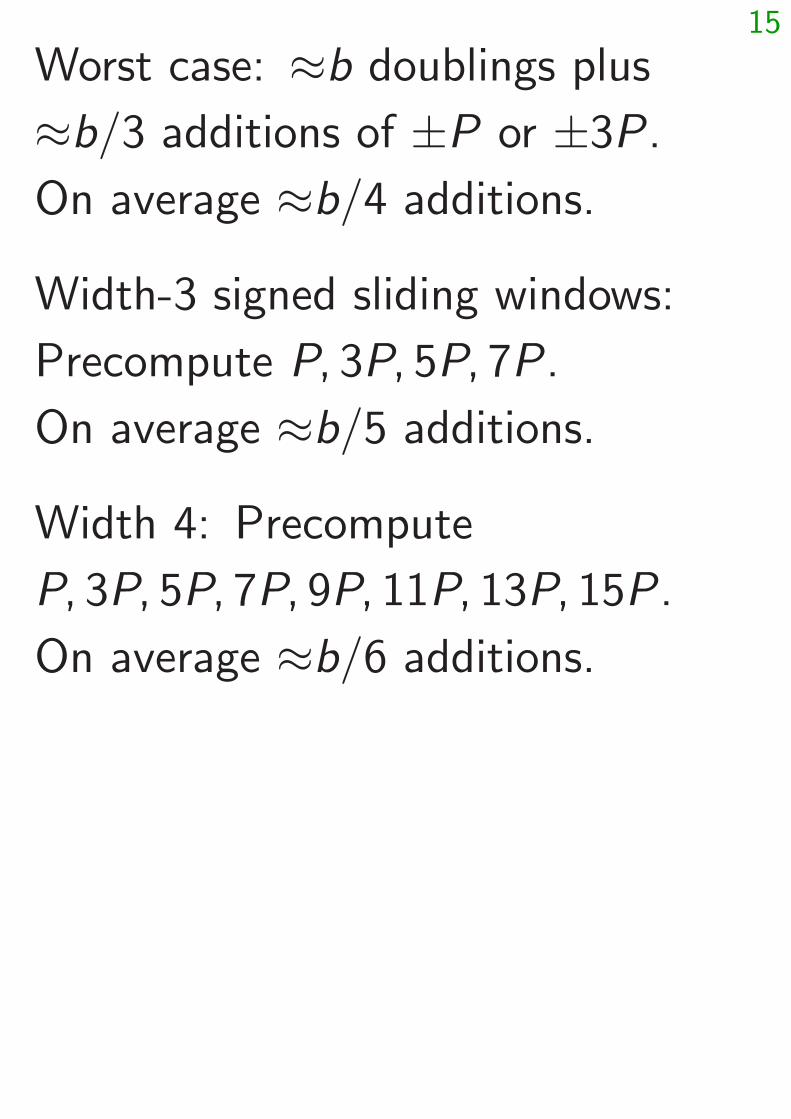
Worst case: ≈b doublings plus
≈b=3 additions of ±P or ±3P .
On average ≈b=4 additions.
Width-3 signed sliding windows:
Precompute P; 3P; 5P; 7P .
On average ≈b=5 additions.
Width 4: Precompute
P; 3P; 5P; 7P; 9P; 11P; 13P; 15P .
On average ≈b=6 additions.
15
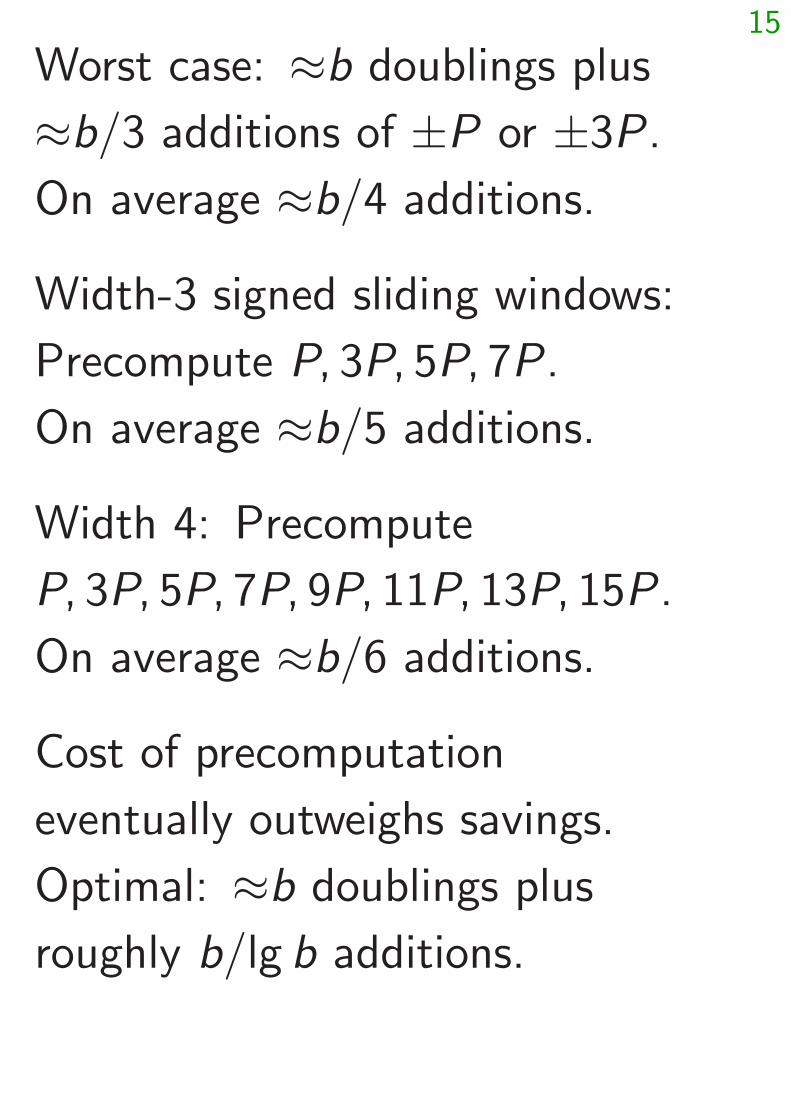
Worst case: ≈b doublings plus
≈b=3 additions of ±P or ±3P .
On average ≈b=4 additions.
Width-3 signed sliding windows:
Precompute P; 3P; 5P; 7P .
On average ≈b=5 additions.
Width 4: Precompute
P; 3P; 5P; 7P; 9P; 11P; 13P; 15P .
On average ≈b=6 additions.
Cost of precomputation
eventually outweighs savings.
Optimal: ≈b doublings plus
roughly b=lg b additions.
16
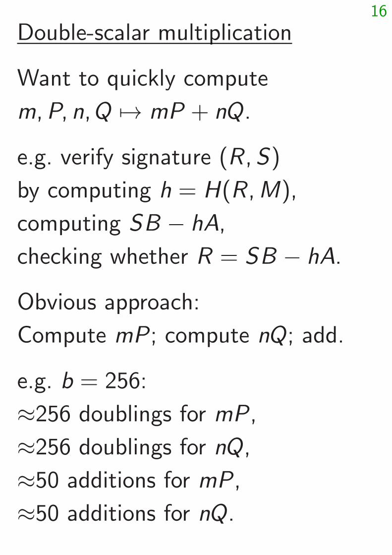
Double-scalar multiplication
Want to quickly compute
m;P; n;Q 7→ mP + nQ.
e.g. verify signature (R; S)
by computing h = H(R;M),
computing SB − hA,
checking whether R = SB − hA.
Obvious approach:
Compute mP ; compute nQ; add.
e.g. b = 256:
≈256 doublings for mP ,
≈256 doublings for nQ,
≈50 additions for mP ,
≈50 additions for nQ.
17
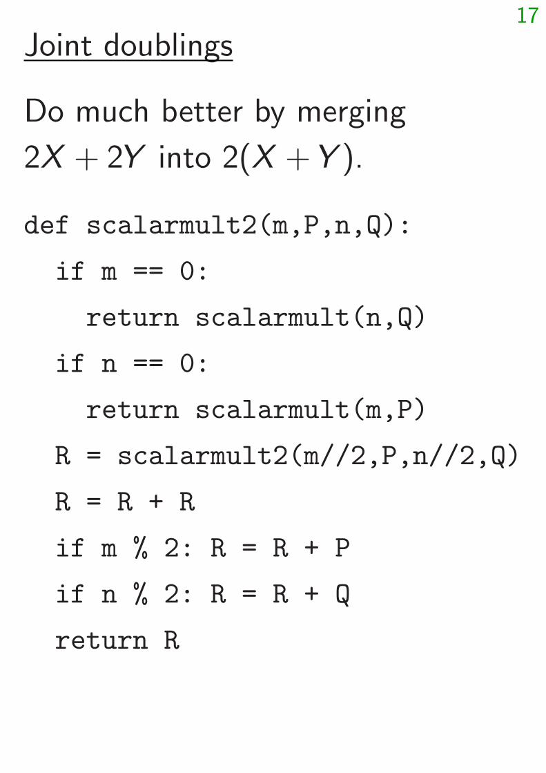
Joint doublings
Do much better by merging
2X + 2Y into 2(X + Y ).
def scalarmult2(m,P,n,Q):
if m == 0:
return scalarmult(n,Q)
if n == 0:
return scalarmult(m,P)
R = scalarmult2(m//2,P,n//2,Q)
R = R + R
if m % 2: R = R + P
if n % 2: R = R + Q
return R
18
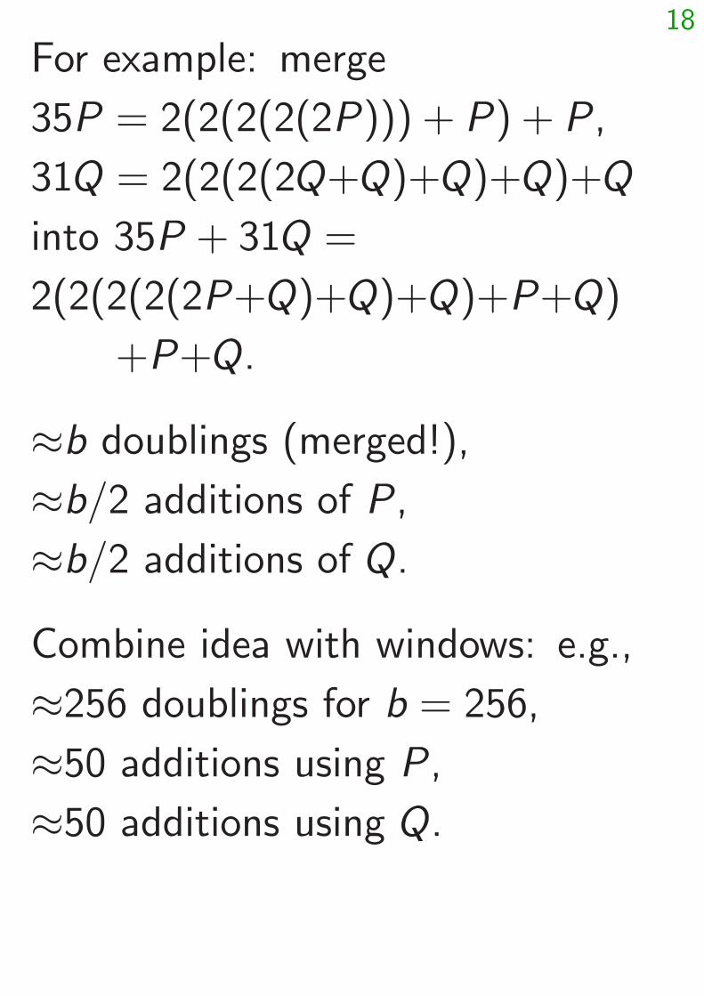
For example: merge
35P = 2(2(2(2(2P ))) + P ) + P ,
31Q = 2(2(2(2Q+Q)+Q)+Q)+Q
into 35P + 31Q =
2(2(2(2(2P+Q)+Q)+Q)+P+Q)
+P+Q.
≈b doublings (merged!),
≈b=2 additions of P ,
≈b=2 additions of Q.
Combine idea with windows: e.g.,
≈256 doublings for b = 256,
≈50 additions using P ,
≈50 additions using Q.
19
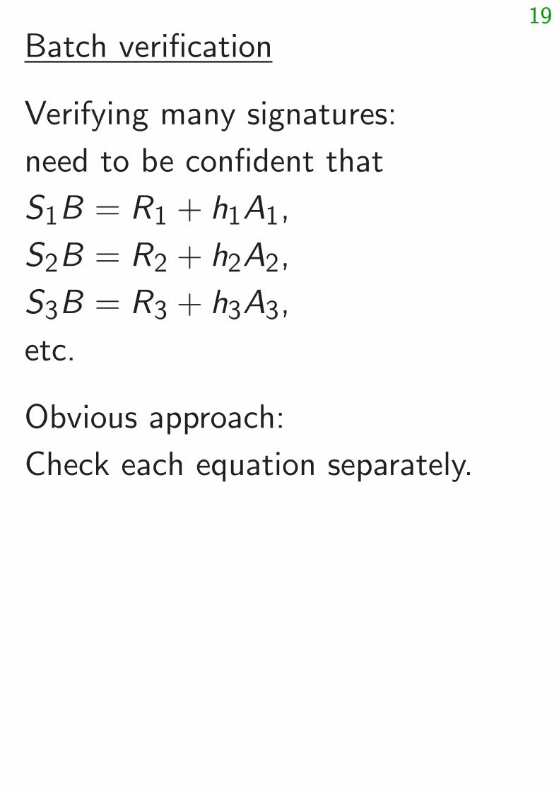
Batch verification
Verifying many signatures:
need to be confident that
S1B = R1 + h1A1,
S2B = R2 + h2A2,
S3B = R3 + h3A3,
etc.
Obvious approach:
Check each equation separately.
19
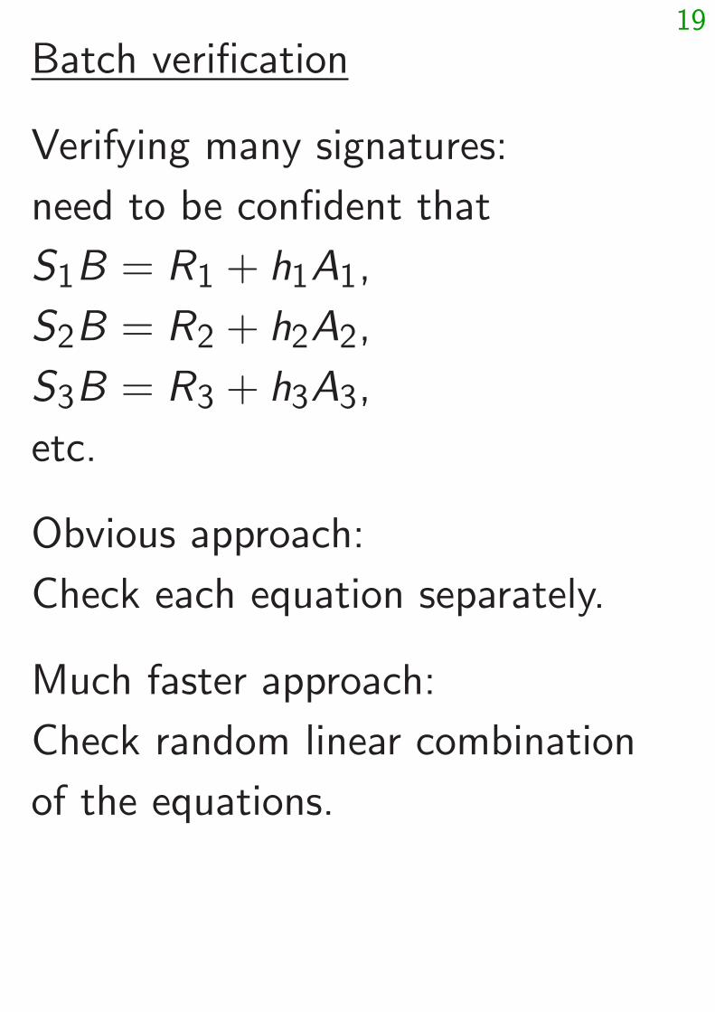
Batch verification
Verifying many signatures:
need to be confident that
S1B = R1 + h1A1,
S2B = R2 + h2A2,
S3B = R3 + h3A3,
etc.
Obvious approach:
Check each equation separately.
Much faster approach:
Check random linear combination
of the equations.
20
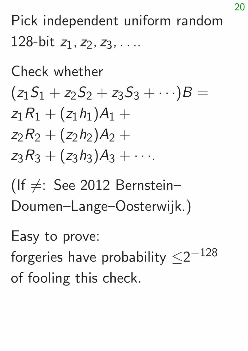
Pick independent uniform random
128-bit z1; z2; z3; : : :.
Check whether
(z1S1 + z2S2 + z3S3 + · · ·)B =
z1R1 + (z1h1)A1 +
z2R2 + (z2h2)A2 +
z3R3 + (z3h3)A3 + · · ·.
(If 6=: See 2012 Bernstein–
Doumen–Lange–Oosterwijk.)
Easy to prove:
forgeries have probability ≤2−128
of fooling this check.
21
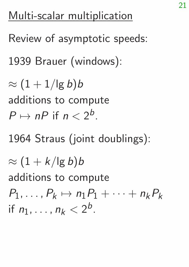
Multi-scalar multiplication
Review of asymptotic speeds:
1939 Brauer (windows):
≈ (1 + 1=lg b)b
additions to compute
P 7→ nP if n < 2b.
1964 Straus (joint doublings):
≈ (1 + k=lg b)b
additions to compute
P1; : : : ; Pk 7→ n1P1 + · · ·+ nkPkif n1; : : : ; nk < 2b.
22
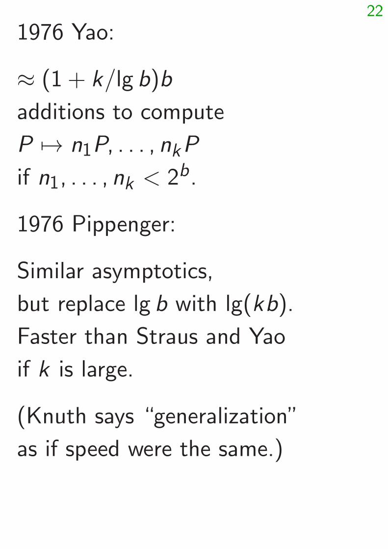
1976 Yao:
≈ (1 + k=lg b)b
additions to compute
P 7→ n1P; : : : ; nkP
if n1; : : : ; nk < 2b.
1976 Pippenger:
Similar asymptotics,
but replace lg b with lg(kb).
Faster than Straus and Yao
if k is large.
(Knuth says “generalization”
as if speed were the same.)
23
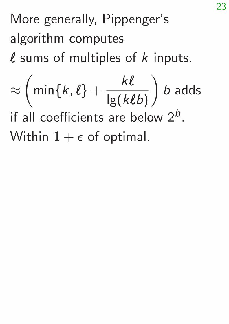
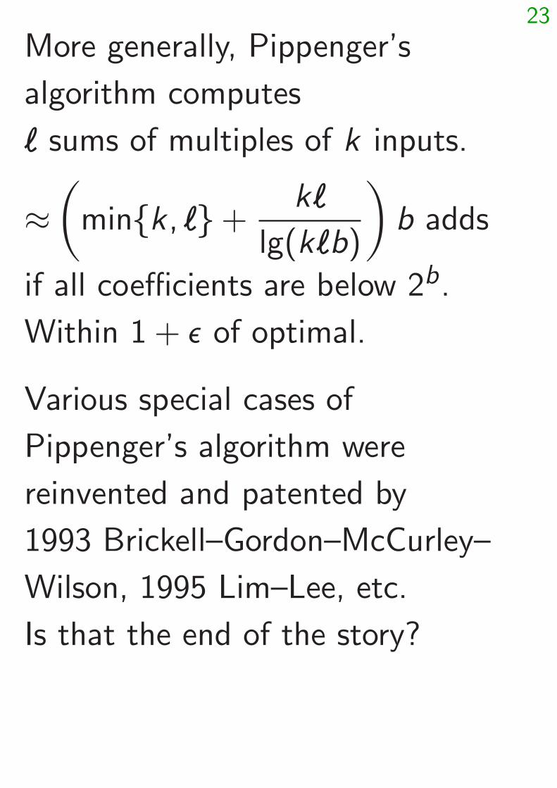
More generally, Pippenger’s
algorithm computes
‘ sums of multiples of k inputs.
≈„
min{k; ‘}+k‘
lg(k‘b)
«b adds
if all coefficients are below 2b.
Within 1 + › of optimal.
23
More generally, Pippenger’s
algorithm computes
‘ sums of multiples of k inputs.
≈„
min{k; ‘}+k‘
lg(k‘b)
«b adds
if all coefficients are below 2b.
Within 1 + › of optimal.
Various special cases of
Pippenger’s algorithm were
reinvented and patented by
1993 Brickell–Gordon–McCurley–
Wilson, 1995 Lim–Lee, etc.
Is that the end of the story?
24
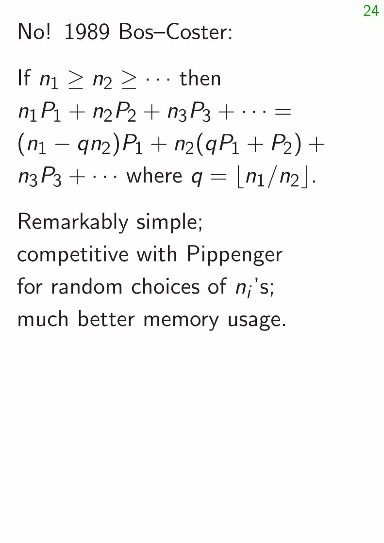
No! 1989 Bos–Coster:
If n1 ≥ n2 ≥ · · · then
n1P1 + n2P2 + n3P3 + · · · =
(n1 − qn2)P1 + n2(qP1 + P2) +
n3P3 + · · · where q = bn1=n2c.
Remarkably simple;
competitive with Pippenger
for random choices of ni ’s;
much better memory usage.
25
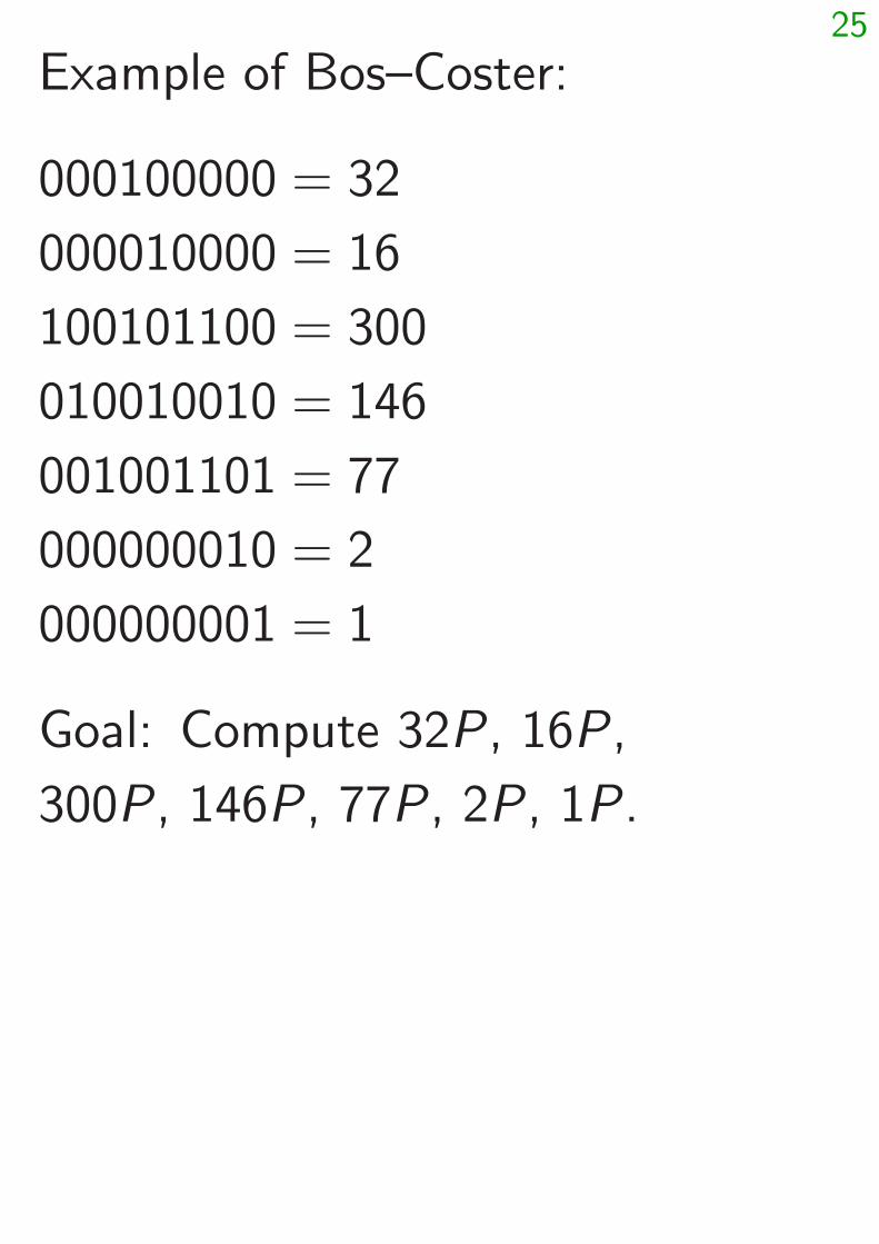
Example of Bos–Coster:
000100000 = 32
000010000 = 16
100101100 = 300
010010010 = 146
001001101 = 77
000000010 = 2
000000001 = 1
Goal: Compute 32P , 16P ,
300P , 146P , 77P , 2P , 1P .
26
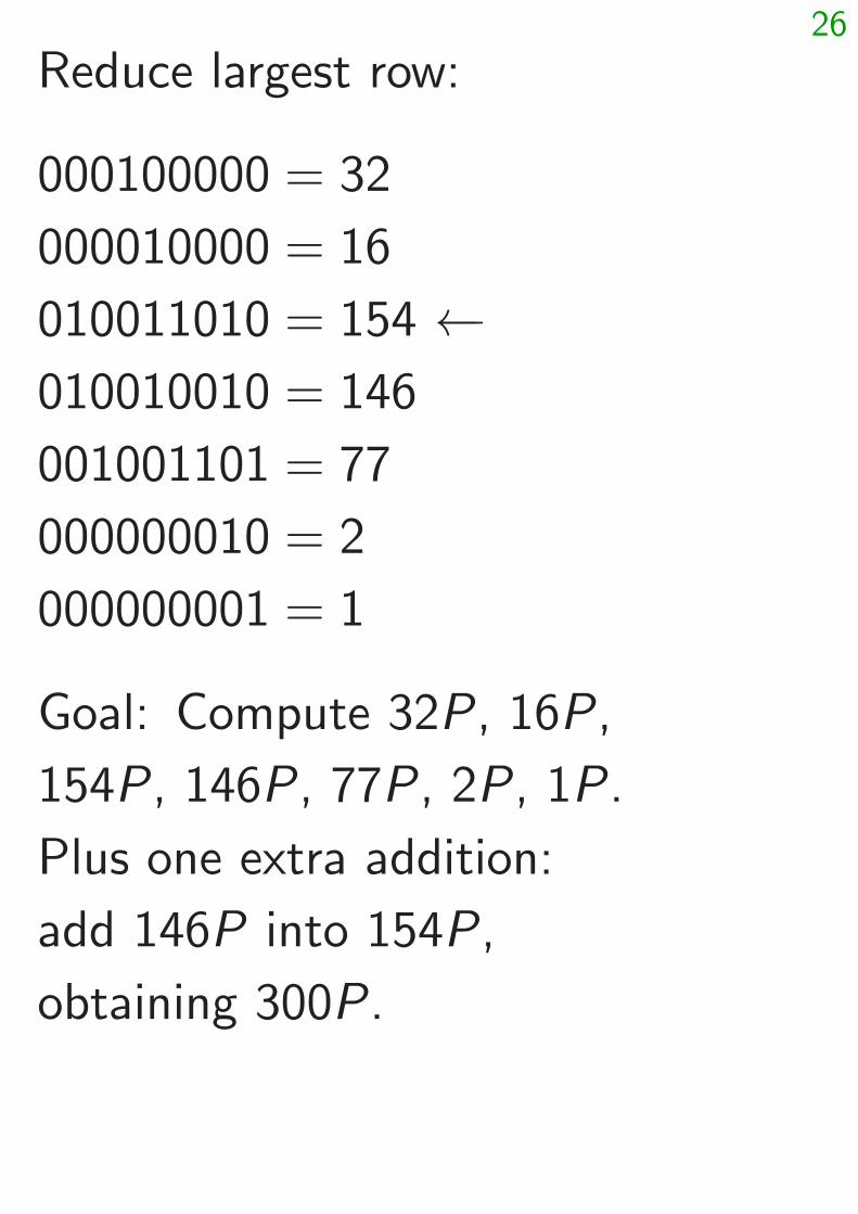
Reduce largest row:
000100000 = 32
000010000 = 16
010011010 = 154 ←010010010 = 146
001001101 = 77
000000010 = 2
000000001 = 1
Goal: Compute 32P , 16P ,
154P , 146P , 77P , 2P , 1P .
Plus one extra addition:
add 146P into 154P ,
obtaining 300P .
26
Reduce largest row:
000100000 = 32
000010000 = 16
000001000 = 8 ←010010010 = 146
001001101 = 77
000000010 = 2
000000001 = 1
plus 2 additions.
26
Reduce largest row:
000100000 = 32
000010000 = 16
000001000 = 8
001000101 = 69 ←001001101 = 77
000000010 = 2
000000001 = 1
plus 3 additions.
26
Reduce largest row:
000100000 = 32
000010000 = 16
000001000 = 8
001000101 = 69
000001000 = 8 ←000000010 = 2
000000001 = 1
plus 4 additions.

26
Reduce largest row:
000100000 = 32
000010000 = 16
000001000 = 8
000100101 = 37 ←000001000 = 8
000000010 = 2
000000001 = 1
plus 5 additions.

26
Reduce largest row:
000100000 = 32
000010000 = 16
000001000 = 8
000000101 = 5 ←000001000 = 8
000000010 = 2
000000001 = 1
plus 6 additions.
26
Reduce largest row:
000010000 = 16 ←000010000 = 16
000001000 = 8
000000101 = 5
000001000 = 8
000000010 = 2
000000001 = 1
plus 7 additions.

26
Reduce largest row:
000000000 = 0
000010000 = 16
000001000 = 8
000000101 = 5
000001000 = 8
000000010 = 2
000000001 = 1
plus 7 additions.

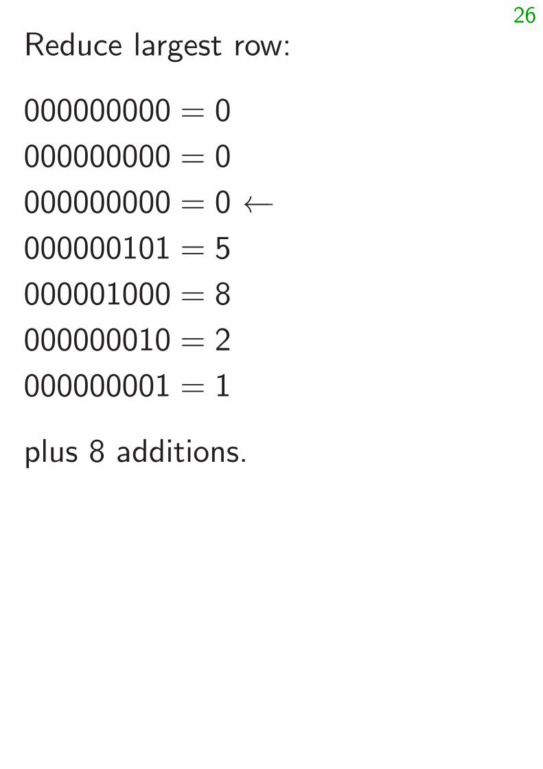
26
Reduce largest row:
000000000 = 0
000001000 = 8 ←000001000 = 8
000000101 = 5
000001000 = 8
000000010 = 2
000000001 = 1
plus 8 additions.

26
Reduce largest row:
000000000 = 0
000000000 = 0 ←000001000 = 8
000000101 = 5
000001000 = 8
000000010 = 2
000000001 = 1
plus 8 additions.
26
Reduce largest row:
000000000 = 0
000000000 = 0
000000000 = 0 ←000000101 = 5
000001000 = 8
000000010 = 2
000000001 = 1
plus 8 additions.

26
Reduce largest row:
000000000 = 0
000000000 = 0
000000000 = 0
000000101 = 5
000000011 = 3 ←000000010 = 2
000000001 = 1
plus 9 additions.
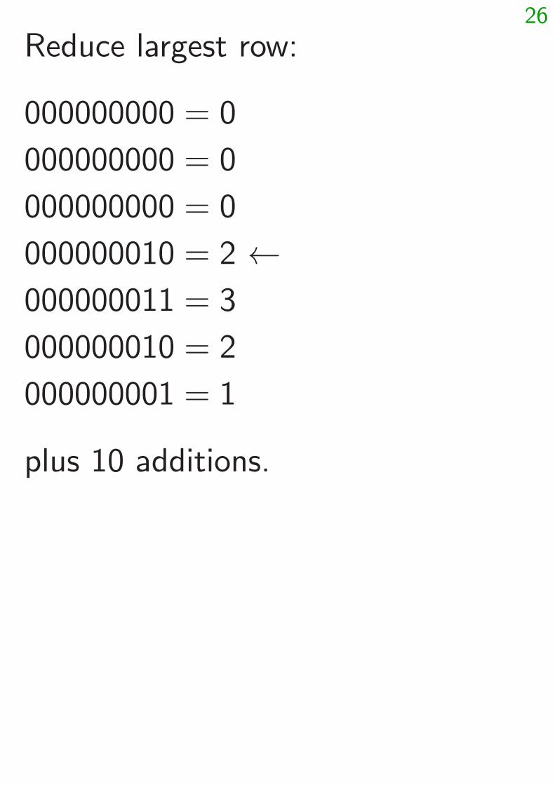
26
Reduce largest row:
000000000 = 0
000000000 = 0
000000000 = 0
000000010 = 2 ←000000011 = 3
000000010 = 2
000000001 = 1
plus 10 additions.

26
Reduce largest row:
000000000 = 0
000000000 = 0
000000000 = 0
000000010 = 2
000000001 = 1 ←000000010 = 2
000000001 = 1
plus 11 additions.

26
Reduce largest row:
000000000 = 0
000000000 = 0
000000000 = 0
000000000 = 0 ←000000001 = 1
000000010 = 2
000000001 = 1
plus 11 additions.
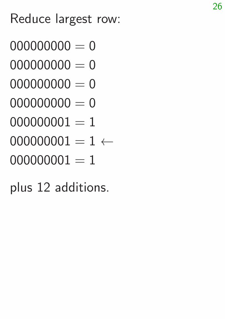
26
Reduce largest row:
000000000 = 0
000000000 = 0
000000000 = 0
000000000 = 0
000000001 = 1
000000001 = 1 ←000000001 = 1
plus 12 additions.
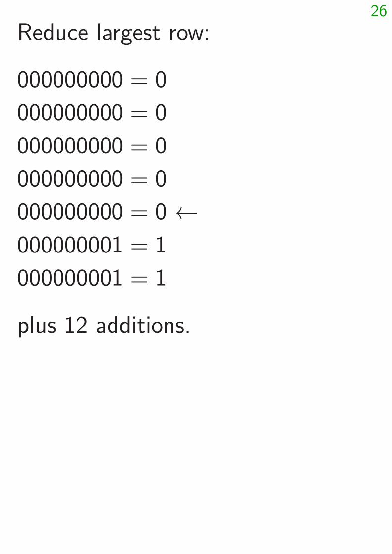
26
Reduce largest row:
000000000 = 0
000000000 = 0
000000000 = 0
000000000 = 0
000000000 = 0 ←000000001 = 1
000000001 = 1
plus 12 additions.
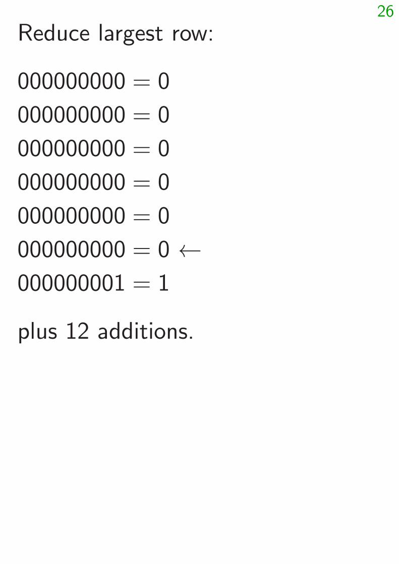
26
Reduce largest row:
000000000 = 0
000000000 = 0
000000000 = 0
000000000 = 0
000000000 = 0
000000000 = 0 ←000000001 = 1
plus 12 additions.
26
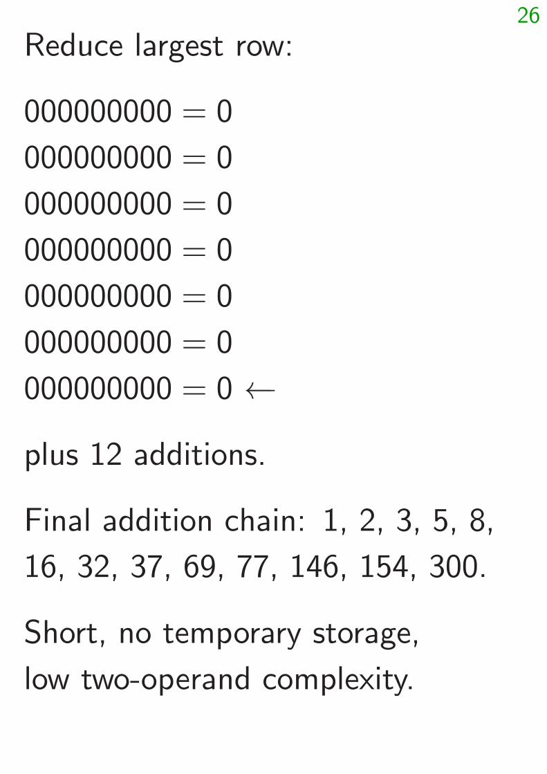
Reduce largest row:
000000000 = 0
000000000 = 0
000000000 = 0
000000000 = 0
000000000 = 0
000000000 = 0
000000000 = 0 ←
plus 12 additions.
Final addition chain: 1, 2, 3, 5, 8,
16, 32, 37, 69, 77, 146, 154, 300.
Short, no temporary storage,
low two-operand complexity.
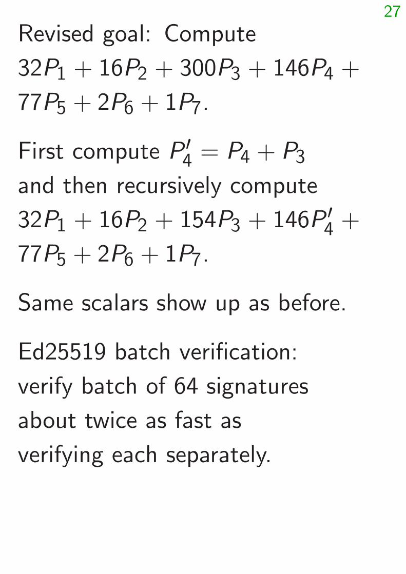
27
Revised goal: Compute
32P1 + 16P2 + 300P3 + 146P4 +
77P5 + 2P6 + 1P7.
First compute P ′4 = P4 + P3
and then recursively compute
32P1 + 16P2 + 154P3 + 146P ′4 +
77P5 + 2P6 + 1P7.
Same scalars show up as before.
Ed25519 batch verification:
verify batch of 64 signatures
about twice as fast as
verifying each separately.