Embed Size (px)
Citation preview
Least Squares Data FittingExistence, Uniqueness, and Conditioning
Solving Linear Least Squares Problems
Scientific Computing: An Introductory SurveyChapter 3 – Linear Least Squares
Prof. Michael T. Heath
Department of Computer ScienceUniversity of Illinois at Urbana-Champaign
Copyright c© 2002. Reproduction permittedfor noncommercial, educational use only.
Michael T. Heath Scientific Computing 1 / 61
Least Squares Data FittingExistence, Uniqueness, and Conditioning
Solving Linear Least Squares Problems
Outline
1 Least Squares Data Fitting
2 Existence, Uniqueness, and Conditioning
3 Solving Linear Least Squares Problems
Michael T. Heath Scientific Computing 2 / 61
Least Squares Data FittingExistence, Uniqueness, and Conditioning
Solving Linear Least Squares Problems
Least SquaresData Fitting
Method of Least Squares
Measurement errors are inevitable in observational andexperimental sciences
Errors can be smoothed out by averaging over manycases, i.e., taking more measurements than are strictlynecessary to determine parameters of system
Resulting system is overdetermined, so usually there is noexact solution
In effect, higher dimensional data are projected into lowerdimensional space to suppress irrelevant detail
Such projection is most conveniently accomplished bymethod of least squares
Michael T. Heath Scientific Computing 3 / 61
Least Squares Data FittingExistence, Uniqueness, and Conditioning
Solving Linear Least Squares Problems
Least SquaresData Fitting
Linear Least Squares
For linear problems, we obtain overdetermined linearsystem Ax = b, with m× n matrix A, m > n
System is better written Ax ∼= b, since equality is usuallynot exactly satisfiable when m > n
Least squares solution x minimizes squared Euclideannorm of residual vector r = b−Ax,
minx‖r‖22 = min
x‖b−Ax‖22
Michael T. Heath Scientific Computing 4 / 61
Least Squares Data FittingExistence, Uniqueness, and Conditioning
Solving Linear Least Squares Problems
Least SquaresData Fitting
Data Fitting
Given m data points (ti, yi), find n-vector x of parametersthat gives “best fit” to model function f(t,x),
minx
m∑i=1
(yi − f(ti,x))2
Problem is linear if function f is linear in components of x,
f(t,x) = x1φ1(t) + x2φ2(t) + · · ·+ xnφn(t)
where functions φj depend only on t
Problem can be written in matrix form as Ax ∼= b, withaij = φj(ti) and bi = yi
Michael T. Heath Scientific Computing 5 / 61
Least Squares Data FittingExistence, Uniqueness, and Conditioning
Solving Linear Least Squares Problems
Least SquaresData Fitting
Data Fitting
Polynomial fitting
f(t,x) = x1 + x2t+ x3t2 + · · ·+ xnt
n−1
is linear, since polynomial linear in coefficients, thoughnonlinear in independent variable t
Fitting sum of exponentials
f(t,x) = x1ex2t + · · ·+ xn−1e
xnt
is example of nonlinear problem
For now, we will consider only linear least squaresproblems
Michael T. Heath Scientific Computing 6 / 61
Least Squares Data FittingExistence, Uniqueness, and Conditioning
Solving Linear Least Squares Problems
Least SquaresData Fitting
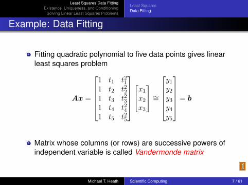
Example: Data Fitting
Fitting quadratic polynomial to five data points gives linearleast squares problem
Ax =
1 t1 t211 t2 t221 t3 t231 t4 t241 t5 t25
x1x2x3
∼=y1y2y3y4y5
= b
Matrix whose columns (or rows) are successive powers ofindependent variable is called Vandermonde matrix
Michael T. Heath Scientific Computing 7 / 61
Least Squares Data FittingExistence, Uniqueness, and Conditioning
Solving Linear Least Squares Problems
Least SquaresData Fitting
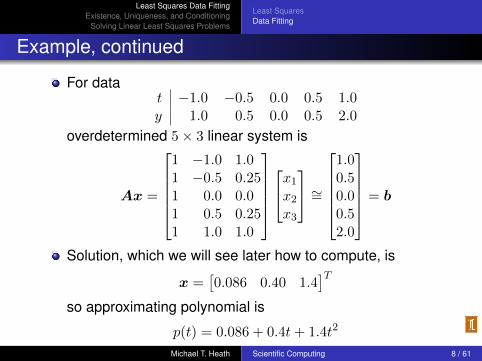
Example, continued
For datat −1.0 −0.5 0.0 0.5 1.0y 1.0 0.5 0.0 0.5 2.0
overdetermined 5× 3 linear system is
Ax =
1 −1.0 1.01 −0.5 0.251 0.0 0.01 0.5 0.251 1.0 1.0
x1x2x3
∼=
1.00.50.00.52.0
= b
Solution, which we will see later how to compute, is
x =[0.086 0.40 1.4
]Tso approximating polynomial is
p(t) = 0.086 + 0.4t+ 1.4t2
Michael T. Heath Scientific Computing 8 / 61
Least Squares Data FittingExistence, Uniqueness, and Conditioning
Solving Linear Least Squares Problems
Least SquaresData Fitting
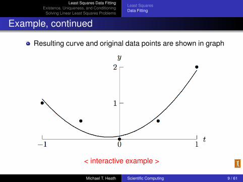
Example, continued
Resulting curve and original data points are shown in graph
< interactive example >
Michael T. Heath Scientific Computing 9 / 61
Least Squares Data FittingExistence, Uniqueness, and Conditioning
Solving Linear Least Squares Problems
Existence and UniquenessOrthogonalityConditioning
Existence and Uniqueness
Linear least squares problem Ax ∼= b always has solution
Solution is unique if, and only if, columns of A are linearlyindependent, i.e., rank(A) = n, where A is m× n
If rank(A) < n, then A is rank-deficient, and solution oflinear least squares problem is not unique
For now, we assume A has full column rank n
Michael T. Heath Scientific Computing 10 / 61

Least Squares Data FittingExistence, Uniqueness, and Conditioning
Solving Linear Least Squares Problems
Existence and UniquenessOrthogonalityConditioning
Normal Equations
To minimize squared Euclidean norm of residual vector
‖r‖22 = rTr = (b−Ax)T (b−Ax)
= bTb− 2xTATb + xTATAx
take derivative with respect to x and set it to 0,
2ATAx− 2ATb = 0
which reduces to n× n linear system of normal equations
ATAx = ATb
Michael T. Heath Scientific Computing 11 / 61
Least Squares Data FittingExistence, Uniqueness, and Conditioning
Solving Linear Least Squares Problems
Existence and UniquenessOrthogonalityConditioning
Orthogonality
Vectors v1 and v2 are orthogonal if their inner product iszero, vT1 v2 = 0
Space spanned by columns of m× n matrix A,span(A) = {Ax : x ∈ Rn}, is of dimension at most n
If m > n, b generally does not lie in span(A), so there is noexact solution to Ax = b
Vector y = Ax in span(A) closest to b in 2-norm occurswhen residual r = b−Ax is orthogonal to span(A),
0 = ATr = AT (b−Ax)
again giving system of normal equations
ATAx = ATb
Michael T. Heath Scientific Computing 12 / 61
Least Squares Data FittingExistence, Uniqueness, and Conditioning
Solving Linear Least Squares Problems
Existence and UniquenessOrthogonalityConditioning
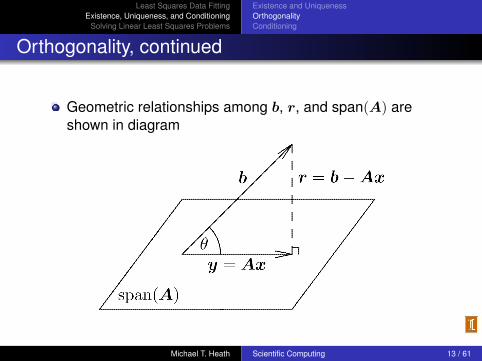
Orthogonality, continued
Geometric relationships among b, r, and span(A) areshown in diagram
Michael T. Heath Scientific Computing 13 / 61
Least Squares Data FittingExistence, Uniqueness, and Conditioning
Solving Linear Least Squares Problems
Existence and UniquenessOrthogonalityConditioning
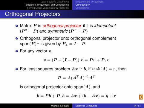
Orthogonal Projectors
Matrix P is orthogonal projector if it is idempotent(P 2 = P ) and symmetric (P T = P )
Orthogonal projector onto orthogonal complementspan(P )⊥ is given by P⊥ = I − P
For any vector v,
v = (P + (I − P )) v = Pv + P⊥v
For least squares problem Ax ∼= b, if rank(A) = n, then
P = A(ATA)−1AT
is orthogonal projector onto span(A), and
b = Pb + P⊥b = Ax + (b−Ax) = y + r
Michael T. Heath Scientific Computing 14 / 61
Least Squares Data FittingExistence, Uniqueness, and Conditioning
Solving Linear Least Squares Problems
Existence and UniquenessOrthogonalityConditioning
Pseudoinverse and Condition Number
Nonsquare m× n matrix A has no inverse in usual sense
If rank(A) = n, pseudoinverse is defined by
A+ = (ATA)−1AT
and condition number by
cond(A) = ‖A‖2 · ‖A+‖2
By convention, cond(A) =∞ if rank(A) < n
Just as condition number of square matrix measurescloseness to singularity, condition number of rectangularmatrix measures closeness to rank deficiency
Least squares solution of Ax ∼= b is given by x = A+ b
Michael T. Heath Scientific Computing 15 / 61
Least Squares Data FittingExistence, Uniqueness, and Conditioning
Solving Linear Least Squares Problems
Existence and UniquenessOrthogonalityConditioning
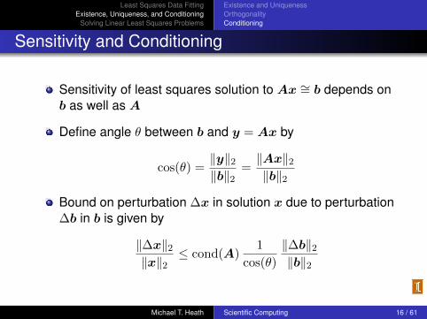
Sensitivity and Conditioning
Sensitivity of least squares solution to Ax ∼= b depends onb as well as A
Define angle θ between b and y = Ax by
cos(θ) =‖y‖2‖b‖2
=‖Ax‖2‖b‖2
Bound on perturbation ∆x in solution x due to perturbation∆b in b is given by
‖∆x‖2‖x‖2
≤ cond(A)1
cos(θ)
‖∆b‖2‖b‖2
Michael T. Heath Scientific Computing 16 / 61
Least Squares Data FittingExistence, Uniqueness, and Conditioning
Solving Linear Least Squares Problems
Existence and UniquenessOrthogonalityConditioning
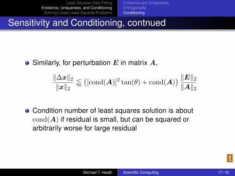
Sensitivity and Conditioning, contnued
Similarly, for perturbation E in matrix A,
‖∆x‖2‖x‖2
/([cond(A)]2 tan(θ) + cond(A)
) ‖E‖2‖A‖2
Condition number of least squares solution is aboutcond(A) if residual is small, but can be squared orarbitrarily worse for large residual
Michael T. Heath Scientific Computing 17 / 61
Least Squares Data FittingExistence, Uniqueness, and Conditioning
Solving Linear Least Squares Problems
Normal EquationsOrthogonal MethodsSVD
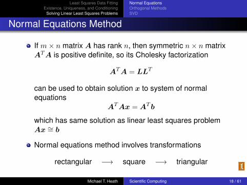
Normal Equations Method
If m× n matrix A has rank n, then symmetric n× n matrixATA is positive definite, so its Cholesky factorization
ATA = LLT
can be used to obtain solution x to system of normalequations
ATAx = ATb
which has same solution as linear least squares problemAx ∼= b
Normal equations method involves transformations
rectangular −→ square −→ triangular
Michael T. Heath Scientific Computing 18 / 61
Least Squares Data FittingExistence, Uniqueness, and Conditioning
Solving Linear Least Squares Problems
Normal EquationsOrthogonal MethodsSVD
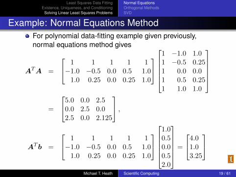
Example: Normal Equations MethodFor polynomial data-fitting example given previously,normal equations method gives
ATA =
1 1 1 1 1−1.0 −0.5 0.0 0.5 1.0
1.0 0.25 0.0 0.25 1.0
1 −1.0 1.01 −0.5 0.251 0.0 0.01 0.5 0.251 1.0 1.0
=
5.0 0.0 2.50.0 2.5 0.02.5 0.0 2.125
,
ATb =
1 1 1 1 1−1.0 −0.5 0.0 0.5 1.0
1.0 0.25 0.0 0.25 1.0
1.00.50.00.52.0
=
4.01.03.25
Michael T. Heath Scientific Computing 19 / 61
Least Squares Data FittingExistence, Uniqueness, and Conditioning
Solving Linear Least Squares Problems
Normal EquationsOrthogonal MethodsSVD
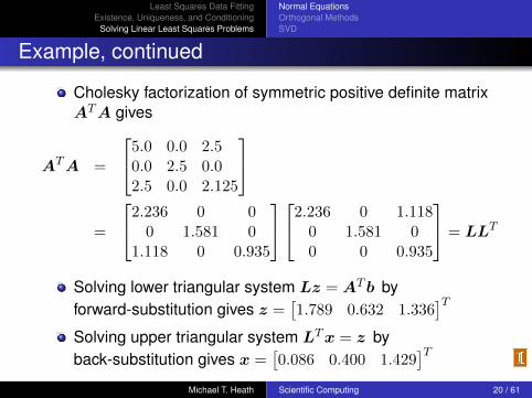
Example, continued
Cholesky factorization of symmetric positive definite matrixATA gives
ATA =
5.0 0.0 2.50.0 2.5 0.02.5 0.0 2.125
=
2.236 0 00 1.581 0
1.118 0 0.935
2.236 0 1.1180 1.581 00 0 0.935
= LLT
Solving lower triangular system Lz = ATb byforward-substitution gives z =
[1.789 0.632 1.336
]TSolving upper triangular system LTx = z byback-substitution gives x =
[0.086 0.400 1.429
]TMichael T. Heath Scientific Computing 20 / 61
Least Squares Data FittingExistence, Uniqueness, and Conditioning
Solving Linear Least Squares Problems
Normal EquationsOrthogonal MethodsSVD
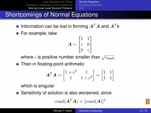
Shortcomings of Normal Equations
Information can be lost in forming ATA and ATb
For example, take
A =
1 1ε 00 ε
where ε is positive number smaller than
√εmach
Then in floating-point arithmetic
ATA =
[1 + ε2 1
1 1 + ε2
]=
[1 11 1
]which is singularSensitivity of solution is also worsened, since
cond(ATA) = [cond(A)]2
Michael T. Heath Scientific Computing 21 / 61
Least Squares Data FittingExistence, Uniqueness, and Conditioning
Solving Linear Least Squares Problems
Normal EquationsOrthogonal MethodsSVD
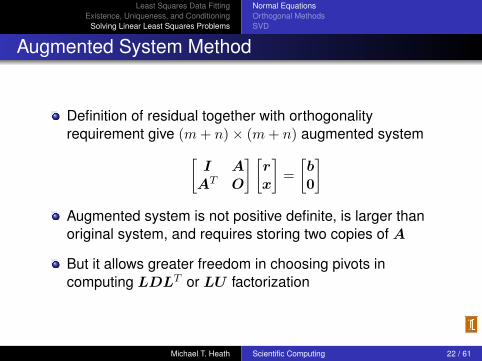
Augmented System Method
Definition of residual together with orthogonalityrequirement give (m+ n)× (m+ n) augmented system[
I AAT O
] [rx
]=
[b0
]Augmented system is not positive definite, is larger thanoriginal system, and requires storing two copies of A
But it allows greater freedom in choosing pivots incomputing LDLT or LU factorization
Michael T. Heath Scientific Computing 22 / 61

Least Squares Data FittingExistence, Uniqueness, and Conditioning
Solving Linear Least Squares Problems
Normal EquationsOrthogonal MethodsSVD
Augmented System Method, continued
Introducing scaling parameter α gives system[αI AAT O
] [r/αx
]=
[b0
]which allows control over relative weights of twosubsystems in choosing pivots
Reasonable rule of thumb is to take
α = maxi,j|aij |/1000
Augmented system is sometimes useful, but is far fromideal in work and storage required
Michael T. Heath Scientific Computing 23 / 61
Least Squares Data FittingExistence, Uniqueness, and Conditioning
Solving Linear Least Squares Problems
Normal EquationsOrthogonal MethodsSVD
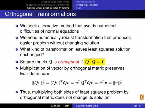
Orthogonal Transformations
We seek alternative method that avoids numericaldifficulties of normal equationsWe need numerically robust transformation that produceseasier problem without changing solutionWhat kind of transformation leaves least squares solutionunchanged?
Square matrix Q is orthogonal if QTQ = I
Multiplication of vector by orthogonal matrix preservesEuclidean norm
‖Qv‖22 = (Qv)TQv = vTQTQv = vTv = ‖v‖22
Thus, multiplying both sides of least squares problem byorthogonal matrix does not change its solution
Michael T. Heath Scientific Computing 24 / 61
Least Squares Data FittingExistence, Uniqueness, and Conditioning
Solving Linear Least Squares Problems
Normal EquationsOrthogonal MethodsSVD
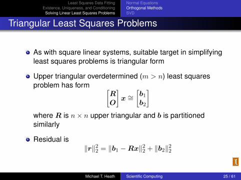
Triangular Least Squares Problems
As with square linear systems, suitable target in simplifyingleast squares problems is triangular form
Upper triangular overdetermined (m > n) least squaresproblem has form [
RO
]x ∼=
[b1b2
]where R is n× n upper triangular and b is partitionedsimilarly
Residual is‖r‖22 = ‖b1 −Rx‖22 + ‖b2‖22
Michael T. Heath Scientific Computing 25 / 61
Least Squares Data FittingExistence, Uniqueness, and Conditioning
Solving Linear Least Squares Problems
Normal EquationsOrthogonal MethodsSVD
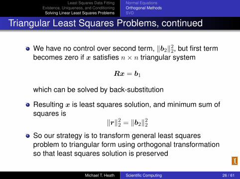
Triangular Least Squares Problems, continued
We have no control over second term, ‖b2‖22, but first termbecomes zero if x satisfies n× n triangular system
Rx = b1
which can be solved by back-substitution
Resulting x is least squares solution, and minimum sum ofsquares is
‖r‖22 = ‖b2‖22So our strategy is to transform general least squaresproblem to triangular form using orthogonal transformationso that least squares solution is preserved
Michael T. Heath Scientific Computing 26 / 61
Least Squares Data FittingExistence, Uniqueness, and Conditioning
Solving Linear Least Squares Problems
Normal EquationsOrthogonal MethodsSVD
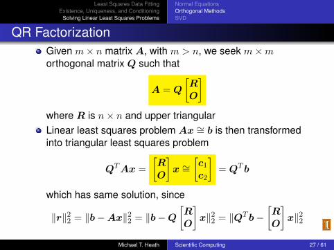
QR FactorizationGiven m× n matrix A, with m > n, we seek m×morthogonal matrix Q such that
A = Q
[RO
]where R is n× n and upper triangularLinear least squares problem Ax ∼= b is then transformedinto triangular least squares problem
QTAx =
[RO
]x ∼=
[c1c2
]= QTb
which has same solution, since
‖r‖22 = ‖b−Ax‖22 = ‖b−Q
[RO
]x‖22 = ‖QTb−
[RO
]x‖22
Michael T. Heath Scientific Computing 27 / 61
Least Squares Data FittingExistence, Uniqueness, and Conditioning
Solving Linear Least Squares Problems
Normal EquationsOrthogonal MethodsSVD
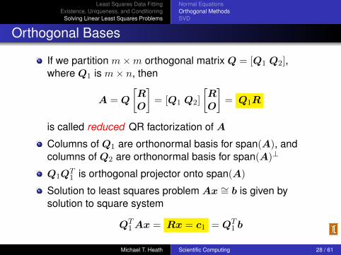
Orthogonal Bases
If we partition m×m orthogonal matrix Q = [Q1 Q2],where Q1 is m× n, then
A = Q
[RO
]= [Q1 Q2]
[RO
]= Q1R
is called reduced QR factorization of A
Columns of Q1 are orthonormal basis for span(A), andcolumns of Q2 are orthonormal basis for span(A)⊥
Q1QT1 is orthogonal projector onto span(A)
Solution to least squares problem Ax ∼= b is given bysolution to square system
QT1 Ax = Rx = c1 = QT
1 b
Michael T. Heath Scientific Computing 28 / 61
Least Squares Data FittingExistence, Uniqueness, and Conditioning
Solving Linear Least Squares Problems
Normal EquationsOrthogonal MethodsSVD
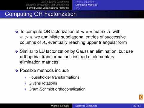
Computing QR Factorization
To compute QR factorization of m× n matrix A, withm > n, we annihilate subdiagonal entries of successivecolumns of A, eventually reaching upper triangular form
Similar to LU factorization by Gaussian elimination, but useorthogonal transformations instead of elementaryelimination matrices
Possible methods include
Householder transformationsGivens rotationsGram-Schmidt orthogonalization
Michael T. Heath Scientific Computing 29 / 61
Least Squares Data FittingExistence, Uniqueness, and Conditioning
Solving Linear Least Squares Problems
Normal EquationsOrthogonal MethodsSVD
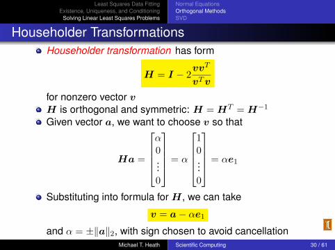
Householder TransformationsHouseholder transformation has form
H = I − 2vvT
vTv
for nonzero vector vH is orthogonal and symmetric: H = HT = H−1
Given vector a, we want to choose v so that
Ha =
α0...0
= α
10...0
= αe1
Substituting into formula for H, we can take
v = a− αe1and α = ±‖a‖2, with sign chosen to avoid cancellation
Michael T. Heath Scientific Computing 30 / 61
Least Squares Data FittingExistence, Uniqueness, and Conditioning
Solving Linear Least Squares Problems
Normal EquationsOrthogonal MethodsSVD
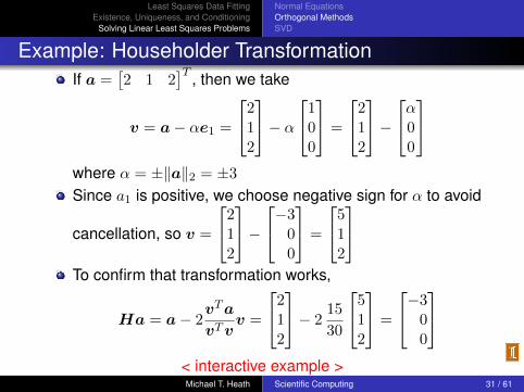
Example: Householder TransformationIf a =
[2 1 2
]T , then we take
v = a− αe1 =
212
− α1
00
=
212
−α0
0
where α = ±‖a‖2 = ±3
Since a1 is positive, we choose negative sign for α to avoid
cancellation, so v =
212
−−3
00
=
512
To confirm that transformation works,
Ha = a− 2vTa
vTvv =
212
− 215
30
512
=
−300
< interactive example >Michael T. Heath Scientific Computing 31 / 61
Least Squares Data FittingExistence, Uniqueness, and Conditioning
Solving Linear Least Squares Problems
Normal EquationsOrthogonal MethodsSVD
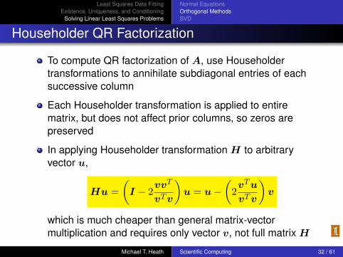
Householder QR Factorization
To compute QR factorization of A, use Householdertransformations to annihilate subdiagonal entries of eachsuccessive column
Each Householder transformation is applied to entirematrix, but does not affect prior columns, so zeros arepreserved
In applying Householder transformation H to arbitraryvector u,
Hu =
(I − 2
vvT
vTv
)u = u−
(2vTu
vTv
)v
which is much cheaper than general matrix-vectormultiplication and requires only vector v, not full matrix H
Michael T. Heath Scientific Computing 32 / 61
Least Squares Data FittingExistence, Uniqueness, and Conditioning
Solving Linear Least Squares Problems
Normal EquationsOrthogonal MethodsSVD
Householder QR Factorization, continued
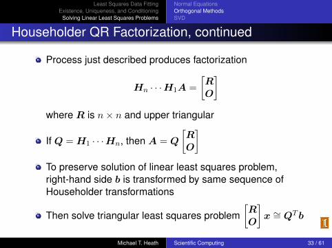
Process just described produces factorization
Hn · · ·H1A =
[RO
]where R is n× n and upper triangular
If Q = H1 · · ·Hn, then A = Q
[RO
]To preserve solution of linear least squares problem,right-hand side b is transformed by same sequence ofHouseholder transformations
Then solve triangular least squares problem[RO
]x ∼= QTb
Michael T. Heath Scientific Computing 33 / 61
Least Squares Data FittingExistence, Uniqueness, and Conditioning
Solving Linear Least Squares Problems
Normal EquationsOrthogonal MethodsSVD
Householder QR Factorization, continued
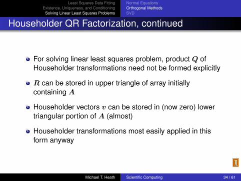
For solving linear least squares problem, product Q ofHouseholder transformations need not be formed explicitly
R can be stored in upper triangle of array initiallycontaining A
Householder vectors v can be stored in (now zero) lowertriangular portion of A (almost)
Householder transformations most easily applied in thisform anyway
Michael T. Heath Scientific Computing 34 / 61
Least Squares Data FittingExistence, Uniqueness, and Conditioning
Solving Linear Least Squares Problems
Normal EquationsOrthogonal MethodsSVD
Example: Householder QR Factorization
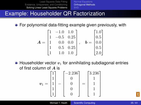
For polynomial data-fitting example given previously, with
A =
1 −1.0 1.01 −0.5 0.251 0.0 0.01 0.5 0.251 1.0 1.0
, b =
1.00.50.00.52.0
Householder vector v1 for annihilating subdiagonal entriesof first column of A is
v1 =
11111
−−2.236
0000
=
3.236
1111
Michael T. Heath Scientific Computing 35 / 61
Least Squares Data FittingExistence, Uniqueness, and Conditioning
Solving Linear Least Squares Problems
Normal EquationsOrthogonal MethodsSVD
Example, continued
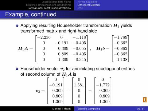
Applying resulting Householder transformation H1 yieldstransformed matrix and right-hand side
H1A =
−2.236 0 −1.118
0 −0.191 −0.4050 0.309 −0.6550 0.809 −0.4050 1.309 0.345
, H1b =
−1.789−0.362−0.862−0.362
1.138
Householder vector v2 for annihilating subdiagonal entriesof second column of H1A is
v2 =
0
−0.1910.3090.8091.309
−
01.581
000
=
0
−1.7720.3090.8091.309
Michael T. Heath Scientific Computing 36 / 61
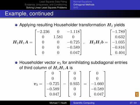
Least Squares Data FittingExistence, Uniqueness, and Conditioning
Solving Linear Least Squares Problems
Normal EquationsOrthogonal MethodsSVD
Example, continued
Applying resulting Householder transformation H2 yields
H2H1A =
−2.236 0 −1.118
0 1.581 00 0 −0.7250 0 −0.5890 0 0.047
, H2H1b =
−1.789
0.632−1.035−0.816
0.404
Householder vector v3 for annihilating subdiagonal entriesof third column of H2H1A is
v3 =
00
−0.725−0.589
0.047
−
00
0.93500
=
00
−1.660−0.589
0.047
Michael T. Heath Scientific Computing 37 / 61
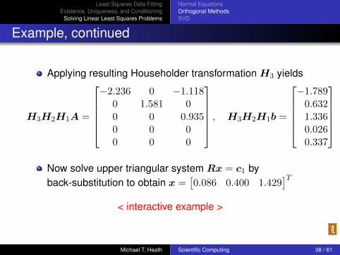
Least Squares Data FittingExistence, Uniqueness, and Conditioning
Solving Linear Least Squares Problems
Normal EquationsOrthogonal MethodsSVD
Example, continued
Applying resulting Householder transformation H3 yields
H3H2H1A =
−2.236 0 −1.118
0 1.581 00 0 0.9350 0 00 0 0
, H3H2H1b =
−1.789
0.6321.3360.0260.337
Now solve upper triangular system Rx = c1 byback-substitution to obtain x =
[0.086 0.400 1.429
]T< interactive example >
Michael T. Heath Scientific Computing 38 / 61
Least Squares Data FittingExistence, Uniqueness, and Conditioning
Solving Linear Least Squares Problems
Normal EquationsOrthogonal MethodsSVD
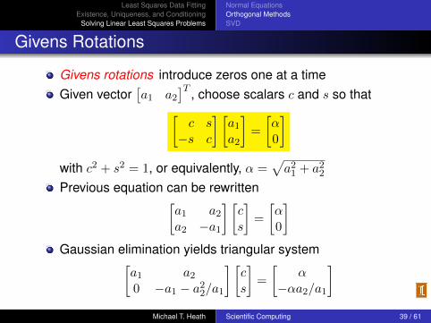
Givens Rotations
Givens rotations introduce zeros one at a timeGiven vector
[a1 a2
]T , choose scalars c and s so that[c s−s c
] [a1a2
]=
[α0
]with c2 + s2 = 1, or equivalently, α =
√a21 + a22
Previous equation can be rewritten[a1 a2a2 −a1
] [cs
]=
[α0
]Gaussian elimination yields triangular system[
a1 a20 −a1 − a22/a1
] [cs
]=
[α
−αa2/a1
]Michael T. Heath Scientific Computing 39 / 61

Least Squares Data FittingExistence, Uniqueness, and Conditioning
Solving Linear Least Squares Problems
Normal EquationsOrthogonal MethodsSVD
Givens Rotations, continued
Back-substitution then gives
s =αa2
a21 + a22and c =
αa1a21 + a22
Finally, c2 + s2 = 1, or α =√a21 + a22, implies
c =a1√a21 + a22
and s =a2√a21 + a22
Michael T. Heath Scientific Computing 40 / 61
Least Squares Data FittingExistence, Uniqueness, and Conditioning
Solving Linear Least Squares Problems
Normal EquationsOrthogonal MethodsSVD
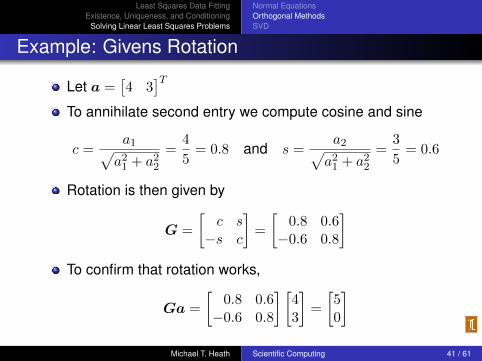
Example: Givens Rotation
Let a =[4 3
]TTo annihilate second entry we compute cosine and sine
c =a1√a21 + a22
=4
5= 0.8 and s =
a2√a21 + a22
=3
5= 0.6
Rotation is then given by
G =
[c s−s c
]=
[0.8 0.6−0.6 0.8
]To confirm that rotation works,
Ga =
[0.8 0.6−0.6 0.8
] [43
]=
[50
]Michael T. Heath Scientific Computing 41 / 61
Least Squares Data FittingExistence, Uniqueness, and Conditioning
Solving Linear Least Squares Problems
Normal EquationsOrthogonal MethodsSVD
Givens QR Factorization
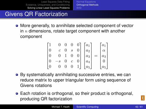
More generally, to annihilate selected component of vectorin n dimensions, rotate target component with anothercomponent
1 0 0 0 00 c 0 s 00 0 1 0 00 −s 0 c 00 0 0 0 1
a1a2a3a4a5
=
a1αa30a5
By systematically annihilating successive entries, we canreduce matrix to upper triangular form using sequence ofGivens rotations
Each rotation is orthogonal, so their product is orthogonal,producing QR factorization
Michael T. Heath Scientific Computing 42 / 61
Least Squares Data FittingExistence, Uniqueness, and Conditioning
Solving Linear Least Squares Problems
Normal EquationsOrthogonal MethodsSVD
Givens QR Factorization
Straightforward implementation of Givens method requiresabout 50% more work than Householder method, and alsorequires more storage, since each rotation requires twonumbers, c and s, to define it
These disadvantages can be overcome, but requires morecomplicated implementation
Givens can be advantageous for computing QRfactorization when many entries of matrix are already zero,since those annihilations can then be skipped
< interactive example >
Michael T. Heath Scientific Computing 43 / 61
Least Squares Data FittingExistence, Uniqueness, and Conditioning
Solving Linear Least Squares Problems
Normal EquationsOrthogonal MethodsSVD
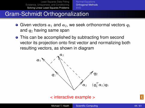
Gram-Schmidt Orthogonalization
Given vectors a1 and a2, we seek orthonormal vectors q1and q2 having same span
This can be accomplished by subtracting from secondvector its projection onto first vector and normalizing bothresulting vectors, as shown in diagram
< interactive example >
Michael T. Heath Scientific Computing 44 / 61

Least Squares Data FittingExistence, Uniqueness, and Conditioning
Solving Linear Least Squares Problems
Normal EquationsOrthogonal MethodsSVD
Gram-Schmidt Orthogonalization
Process can be extended to any number of vectorsa1, . . . ,ak, orthogonalizing each successive vector againstall preceding ones, giving classical Gram-Schmidtprocedure
for k = 1 to nqk = akfor j = 1 to k − 1
rjk = qTj akqk = qk − rjkqj
endrkk = ‖qk‖2qk = qk/rkk
endResulting qk and rjk form reduced QR factorization of A
Michael T. Heath Scientific Computing 45 / 61

Least Squares Data FittingExistence, Uniqueness, and Conditioning
Solving Linear Least Squares Problems
Normal EquationsOrthogonal MethodsSVD
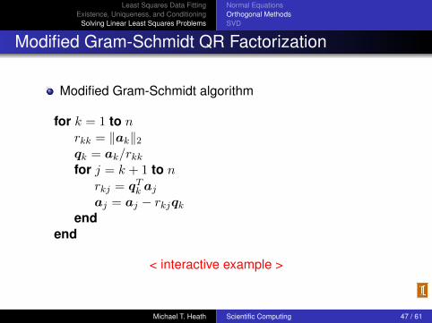
Modified Gram-Schmidt
Classical Gram-Schmidt procedure often suffers loss oforthogonality in finite-precision
Also, separate storage is required for A, Q, and R, sinceoriginal ak are needed in inner loop, so qk cannot overwritecolumns of A
Both deficiencies are improved by modified Gram-Schmidtprocedure, with each vector orthogonalized in turn againstall subsequent vectors, so qk can overwrite ak
Michael T. Heath Scientific Computing 46 / 61
Least Squares Data FittingExistence, Uniqueness, and Conditioning
Solving Linear Least Squares Problems
Normal EquationsOrthogonal MethodsSVD
Modified Gram-Schmidt QR Factorization
Modified Gram-Schmidt algorithm
for k = 1 to nrkk = ‖ak‖2qk = ak/rkkfor j = k + 1 to n
rkj = qTk ajaj = aj − rkjqk
endend
< interactive example >
Michael T. Heath Scientific Computing 47 / 61
Least Squares Data FittingExistence, Uniqueness, and Conditioning
Solving Linear Least Squares Problems
Normal EquationsOrthogonal MethodsSVD
Rank Deficiency
If rank(A) < n, then QR factorization still exists, but yieldssingular upper triangular factor R, and multiple vectors xgive minimum residual norm
Common practice selects minimum residual solution xhaving smallest norm
Can be computed by QR factorization with column pivotingor by singular value decomposition (SVD)
Rank of matrix is often not clear cut in practice, so relativetolerance is used to determine rank
Michael T. Heath Scientific Computing 48 / 61
Least Squares Data FittingExistence, Uniqueness, and Conditioning
Solving Linear Least Squares Problems
Normal EquationsOrthogonal MethodsSVD
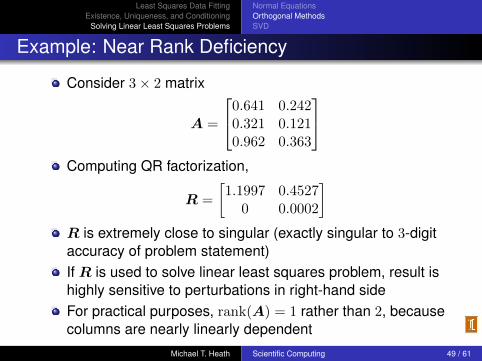
Example: Near Rank Deficiency
Consider 3× 2 matrix
A =
0.641 0.2420.321 0.1210.962 0.363
Computing QR factorization,
R =
[1.1997 0.4527
0 0.0002
]R is extremely close to singular (exactly singular to 3-digitaccuracy of problem statement)If R is used to solve linear least squares problem, result ishighly sensitive to perturbations in right-hand sideFor practical purposes, rank(A) = 1 rather than 2, becausecolumns are nearly linearly dependent
Michael T. Heath Scientific Computing 49 / 61
Least Squares Data FittingExistence, Uniqueness, and Conditioning
Solving Linear Least Squares Problems
Normal EquationsOrthogonal MethodsSVD
QR with Column Pivoting
Instead of processing columns in natural order, select forreduction at each stage column of remaining unreducedsubmatrix having maximum Euclidean norm
If rank(A) = k < n, then after k steps, norms of remainingunreduced columns will be zero (or “negligible” infinite-precision arithmetic) below row k
Yields orthogonal factorization of form
QTAP =
[R SO O
]where R is k × k, upper triangular, and nonsingular, andpermutation matrix P performs column interchanges
Michael T. Heath Scientific Computing 50 / 61
Least Squares Data FittingExistence, Uniqueness, and Conditioning
Solving Linear Least Squares Problems
Normal EquationsOrthogonal MethodsSVD
QR with Column Pivoting, continued
Basic solution to least squares problem Ax ∼= b can nowbe computed by solving triangular system Rz = c1, wherec1 contains first k components of QTb, and then taking
x = P
[z0
]Minimum-norm solution can be computed, if desired, atexpense of additional processing to annihilate S
rank(A) is usually unknown, so rank is determined bymonitoring norms of remaining unreduced columns andterminating factorization when maximum value falls belowchosen tolerance
< interactive example >
Michael T. Heath Scientific Computing 51 / 61
Least Squares Data FittingExistence, Uniqueness, and Conditioning
Solving Linear Least Squares Problems
Normal EquationsOrthogonal MethodsSVD
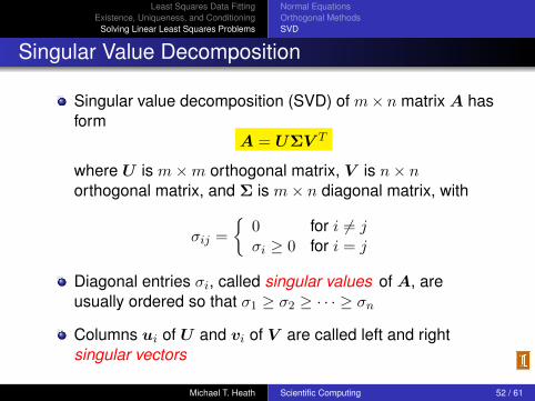
Singular Value Decomposition
Singular value decomposition (SVD) of m× n matrix A hasform
A = UΣV T
where U is m×m orthogonal matrix, V is n× northogonal matrix, and Σ is m× n diagonal matrix, with
σij =
{0 for i 6= jσi ≥ 0 for i = j
Diagonal entries σi, called singular values of A, areusually ordered so that σ1 ≥ σ2 ≥ · · · ≥ σn
Columns ui of U and vi of V are called left and rightsingular vectors
Michael T. Heath Scientific Computing 52 / 61
Least Squares Data FittingExistence, Uniqueness, and Conditioning
Solving Linear Least Squares Problems
Normal EquationsOrthogonal MethodsSVD
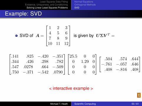
Example: SVD
SVD of A =
1 2 34 5 67 8 910 11 12
is given by UΣV T =
.141 .825 −.420 −.351.344 .426 .298 .782.547 .0278 .664 −.509.750 −.371 −.542 .0790
25.5 0 00 1.29 00 0 00 0 0
.504 .574 .644−.761 −.057 .646.408 −.816 .408
< interactive example >
Michael T. Heath Scientific Computing 53 / 61

Least Squares Data FittingExistence, Uniqueness, and Conditioning
Solving Linear Least Squares Problems
Normal EquationsOrthogonal MethodsSVD
Applications of SVD
Minimum norm solution to Ax ∼= b is given by
x =∑σi 6=0
uTi b
σivi
For ill-conditioned or rank deficient problems, “small”singular values can be omitted from summation to stabilizesolution
Euclidean matrix norm : ‖A‖2 = σmax
Euclidean condition number of matrix : cond(A) =σmax
σmin
Rank of matrix : number of nonzero singular values
Michael T. Heath Scientific Computing 54 / 61
Least Squares Data FittingExistence, Uniqueness, and Conditioning
Solving Linear Least Squares Problems
Normal EquationsOrthogonal MethodsSVD
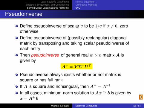
Pseudoinverse
Define pseudoinverse of scalar σ to be 1/σ if σ 6= 0, zerootherwiseDefine pseudoinverse of (possibly rectangular) diagonalmatrix by transposing and taking scalar pseudoinverse ofeach entryThen pseudoinverse of general real m× n matrix A isgiven by
A+ = V Σ+UT
Pseudoinverse always exists whether or not matrix issquare or has full rankIf A is square and nonsingular, then A+ = A−1
In all cases, minimum-norm solution to Ax ∼= b is given byx = A+ b
Michael T. Heath Scientific Computing 55 / 61

Least Squares Data FittingExistence, Uniqueness, and Conditioning
Solving Linear Least Squares Problems
Normal EquationsOrthogonal MethodsSVD
Orthogonal Bases
SVD of matrix, A = UΣV T , provides orthogonal bases forsubspaces relevant to A
Columns of U corresponding to nonzero singular valuesform orthonormal basis for span(A)
Remaining columns of U form orthonormal basis fororthogonal complement span(A)⊥
Columns of V corresponding to zero singular values formorthonormal basis for null space of A
Remaining columns of V form orthonormal basis fororthogonal complement of null space of A
Michael T. Heath Scientific Computing 56 / 61
Least Squares Data FittingExistence, Uniqueness, and Conditioning
Solving Linear Least Squares Problems
Normal EquationsOrthogonal MethodsSVD
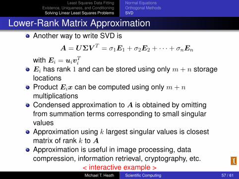
Lower-Rank Matrix ApproximationAnother way to write SVD is
A = UΣV T = σ1E1 + σ2E2 + · · ·+ σnEn
with Ei = uivTi
Ei has rank 1 and can be stored using only m+ n storagelocationsProduct Eix can be computed using only m+ nmultiplicationsCondensed approximation to A is obtained by omittingfrom summation terms corresponding to small singularvaluesApproximation using k largest singular values is closestmatrix of rank k to AApproximation is useful in image processing, datacompression, information retrieval, cryptography, etc.
< interactive example >Michael T. Heath Scientific Computing 57 / 61

Least Squares Data FittingExistence, Uniqueness, and Conditioning
Solving Linear Least Squares Problems
Normal EquationsOrthogonal MethodsSVD
Total Least Squares
Ordinary least squares is applicable when right-hand sideb is subject to random error but matrix A is knownaccurately
When all data, including A, are subject to error, then totalleast squares is more appropriate
Total least squares minimizes orthogonal distances, ratherthan vertical distances, between model and data
Total least squares solution can be computed from SVD of[A, b]
Michael T. Heath Scientific Computing 58 / 61
Least Squares Data FittingExistence, Uniqueness, and Conditioning
Solving Linear Least Squares Problems
Normal EquationsOrthogonal MethodsSVD
Comparison of Methods
Forming normal equations matrix ATA requires aboutn2m/2 multiplications, and solving resulting symmetriclinear system requires about n3/6 multiplications
Solving least squares problem using Householder QRfactorization requires about mn2 − n3/3 multiplications
If m ≈ n, both methods require about same amount ofwork
If m� n, Householder QR requires about twice as muchwork as normal equations
Cost of SVD is proportional to mn2 + n3, withproportionality constant ranging from 4 to 10, depending onalgorithm used
Michael T. Heath Scientific Computing 59 / 61

Least Squares Data FittingExistence, Uniqueness, and Conditioning
Solving Linear Least Squares Problems
Normal EquationsOrthogonal MethodsSVD
Comparison of Methods, continued
Normal equations method produces solution whoserelative error is proportional to [cond(A)]2
Required Cholesky factorization can be expected to breakdown if cond(A) ≈ 1/
√εmach or worse
Householder method produces solution whose relativeerror is proportional to
cond(A) + ‖r‖2 [cond(A)]2
which is best possible, since this is inherent sensitivity ofsolution to least squares problem
Householder method can be expected to break down (inback-substitution phase) only if cond(A) ≈ 1/εmach or worse
Michael T. Heath Scientific Computing 60 / 61
Least Squares Data FittingExistence, Uniqueness, and Conditioning
Solving Linear Least Squares Problems
Normal EquationsOrthogonal MethodsSVD
Comparison of Methods, continued
Householder is more accurate and more broadlyapplicable than normal equations
These advantages may not be worth additional cost,however, when problem is sufficiently well conditioned thatnormal equations provide sufficient accuracy
For rank-deficient or nearly rank-deficient problems,Householder with column pivoting can produce usefulsolution when normal equations method fails outright
SVD is even more robust and reliable than Householder,but substantially more expensive
Michael T. Heath Scientific Computing 61 / 61