Embed Size (px)
Citation preview

Topic 5Knot theory
A First Look at Quantum Physics
2011 Classical Electrodynamics Prof. Y. F. Chen
Scientific Calculation and
Visualization

2011 Classical Electrodynamics
KNOT KNOT & KNOT
2011 Classical Electrodynamics

• BackgroundofKnots
• TorusKnots
• DecorativeKnotPatterns
• KnottedTori
• LissajousKnots
Contents

BACKGROUND OF KNOTSHistory of Knot Theory / Definition of Knot Theory & Knots

Archaeologists have discovered that knottying dates back to prehistoric times.Besides their uses such as recordinginformation and tying objects together,knots have interested humans for theiraesthetics and spiritual symbolism.
§1.1 History of Knot Theory

Mathematical studies of knots began inthe 19th century with Gauss, whodefined the linking integral. In the 1860s,Lord Kelvin's theory that atoms wereknots in the ether led to Peter GuthrieTait's creation of the first knot tables.Tabulation motivated the early knottheorists, but knot theory eventuallybecame part of the emerging subject oftopology.
Knot table
Lord KelvinGauss
§1.1 History of Knot Theory

In the last several decades of the 20th century, scientistsbecame interested in studying physical knots in order tounderstand knotting phenomena in DNA and otherpolymers. Knot theory can be used to determine if amolecule is chiral or not.
Besides, another area for the application of knot theory isstatistical mechanics. This application was leftundiscovered until very recently. Vaughan Jonesdiscovered the connection when computing a newpolynomial invariant for knots. In this field, knots canused to represent systems and thereby increase the ease ofthe study.
§1.1 History of Knot Theory

What is Knot theory ?Knot Theory is a branch of topology that deals with knots and links.
What is a "mathematical" knot?
In mathematics, a knot is an embedding of a circle in 3-dimensional Euclidean space,R3, considered up to continuous deformations (isotopies). A crucial difference betweenthe standard mathematical and conventional notions of a knot is that mathematicalknots are closed—there are no ends to tie or untie on a mathematical knot. Physicalproperties such as friction and thickness also do not apply, although there aremathematical definitions of a knot that take such properties into account. The termknot is also applied to embeddings of Sj in Sn, especially in the case j = n − 2. Thebranch of mathematics that studies knots is known as knot theory.
§1.2 Definition of Knot Theory & Knots

TORUS KNOTS

In knot theory, a torus knot is a special kind of knot that lies on the surface of anunknotted torus in R3. Each torus knot is specified by a pair of coprime integers p and q.The (p,q)-torus knot winds q times around a circle in the interior of the torus, and ptimes around its axis of rotational symmetry. A torus knot is trivial if and only if eitherp or q is equal to 1 or −1. A unknot is also called the trivial knot. The simplestnontrivial example is the (2,3)-torus knot, also known as the trefoil knot.
Two simple diagrams of the unknot Trefoil knot
§2.1 Torus Knots

§2.2.1 Torus
In geometry, a torus (pl. tori) is a surface of revolution generated by revolving acircle in three dimensional space about an axis coplanar with the circle. In mostcontexts it is assumed that the axis does not touch the circle - in this case thesurface has a ring shape and is called a ring torus or simply torus if the ring shape isimplicit.
The parametric equations can be defined as:
θ , φ are in the interval [0, 2π)d : distance from the center of the tube to
the center of the torusa : radius of the tube
d a
, cos cos
, cos sin
, sin
x a d
y a d
z a

§2.2.2 Mathematical Definition of Torus
An implicit equation in Cartesian coordinates for a torus radially symmetric aboutthe z-axis is
2 2 2 2 2( )x y d z a
As the distance to the axis of revolution decreases, the ring torus becomes a spindletorus and then degenerates into a sphere.
When d = 0, the torusdegenerates to the sphere.

sin sin
sin cos
cos
x a q d p
y a q d p
z a q
The (p,q)-torus knot can be given by the parametrization :
§2.3 Mathematical Definition of (p , q) - Torus Knot
2 2 2 2 2( )x y d z a
, 3,5p q
An implicit equation in Cartesian coordinates for a (p,q)-torus knot radiallysymmetric about the z-axis is just the same as the torus :

a=2 d=4 p=1 q is varied
q=3 q=4 q=5q=2
q=7 q=8 q=9q=6
§2.4 Theoretical Simulation of (p , q) - Torus Knot

q=3 q=7 q=11
q=4 q=8
q=5 q=9
q=6 q=10
q=12
q=13
q=14
The same pattern occurs ifthe ratio q/p is identical.
§2.4 Theoretical Simulation of (p , q) - Torus Knot
a=2 d=4 p=2 q is varied

q=4 q=8 q=12
q=5 q=9
q=6 q=10
q=7 q=11
q=13
q=14
q=15
a=2 d=4 p=3 q is varied
§2.4 Theoretical Simulation of (p , q) - Torus Knot
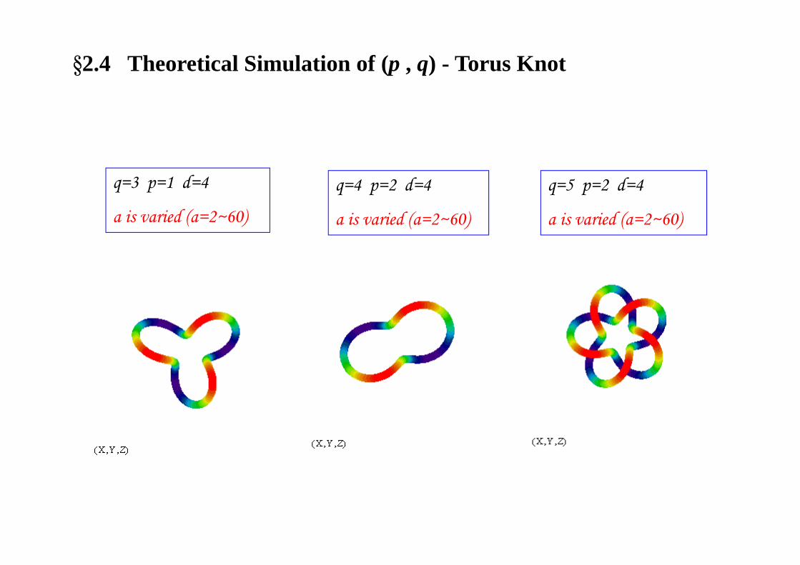
q=3 p=1 d=4
a is varied (a=2~60)
q=4 p=2 d=4
a is varied (a=2~60)
q=5 p=2 d=4
a is varied (a=2~60)
§2.4 Theoretical Simulation of (p , q) - Torus Knot

(q,p)=(3,1)X Y Z( )
X Y Z( )
X Y Z( )
X Y Z( )
X Y Z( )
X Y Z( )
X Y Z( )
X Y Z( )
X Y Z( )
a=3 d=4
a=4 d=4
a=7 d=4
a=8 d=4
a=9 d=4
a=18 d=4
a=25 d=4
a=60 d=4a=5 d=4
X Y Z( ) X Y Z( ) X Y Z( )
a=2 d=4 a=6 d=4 a=12 d=4

X Y Z( )
X Y Z( )
X Y Z( )
X Y Z( )
(q,p)=(4,1)
a=20 d=4
a=30 d=4
a=10 d=4
a=100 d=4
X Y Z( )
X Y Z( )
X Y Z( )
X Y Z( )
a=7 d=4
a=30 d=4
a=100 d=4
a=10 d=4
(q,p)=(4,2)
X Y Z( )
X Y Z( )
X Y Z( )
X Y Z( )
a=15 d=4
a=25 d=4
a=50 d=4
a=10 d=4
(q,p)=(5,2)

§2.5 Different Visual Angle of (1,1) - Torus Knot
X-Y plot X-Z plot

§2.5 Different Visual Angle of (3,4) - Torus Knot
X-Y plot X-Z plot

(5,7) Torus Knot (13,37) Torus Knot
X-Y plot X-Z plot X-Y plot X-Z plot
§2.5 Different Visual Angle of Torus Knots

DECORATIVE KNOT PATTERNS

By Lindsay D Taylor
The approach uses trigonometric parameterizations for the knots and is based on the use ofepitrochoid and hypotrochoid plane curves interlaced by using one or more sin functions inthe 3rd dimension. In its simplest form they can be represented by the following equations.
for p, q are non‐zero integers and p > 0 . When q < 0 the loops faceoutwards, while when q > 0 the loops face inwards.
§3.1 Decorative Knot Patterns
cos cos
sin sin
sin
x m p n q
y m p n q
z h t
0 2

Cycloid Trochoid
§3.2.1 Introduction of Cycloid & Trochoid

Epicycloid
Hypocycloid
§3.2.2 Introduction of Epicycloid & Hypocycloid

Epitrochoid Hypotrochoid
§3.2.3 Introduction of Epitrochoid & Hypotrochoid

Outer Circulating Patterns
(2, 7) Knotx = cos(2*θ) + 0.2*cos(-5* θ)y = sin(2* θ) + 0.2*sin(-5* θ)z = 0.35*sin(7* θ)
(2,9) Knotx = cos(2* θ) + 0.25*cos(-7* θ)y = sin(2* θ) + 0.25*sin(-7* θ)z = 0.35*sin(9* θ)
(2,5)
(2,7)
(2,9)
(2, 5) Knotx = cos(2*θ) + 0.45*cos(-3* θ)y = sin(2* θ) + 0.45*sin(-3* θ)z = 0.35*sin(5* θ)
§3.3 Decorative Knot Patterns

(2,7) (2,9)(2,5)
(2,5) (3,5) (4,5)
§3.3 Decorative Knot Patterns
Outer Circulating Patterns

§3.3 Decorative Knot Patterns
Inner Looping Patterns

§3.3 Decorative Knot Patterns
Inner Looping Patterns

Some Compound Patterns
§3.3 Decorative Knot Patterns

Larger Groupings of Knots
§3.3 Decorative Knot Patterns

KNOTTED TORI

§4.1 Reference Paper of Knotted Tori

, [( sin( ) ) sin( )] sin( )
, [( sin( ) ) cos( )] cos( )
, cos( ) cos( )
x a q d p b p
y a q d p b p
z a q b q
a=5 d=10 q=3 p=2 b is varied (b=1~10)
b=1 b=2
b=5 b=10
§4.2 Mathematical Definition of Knotted Tori
Line Surface
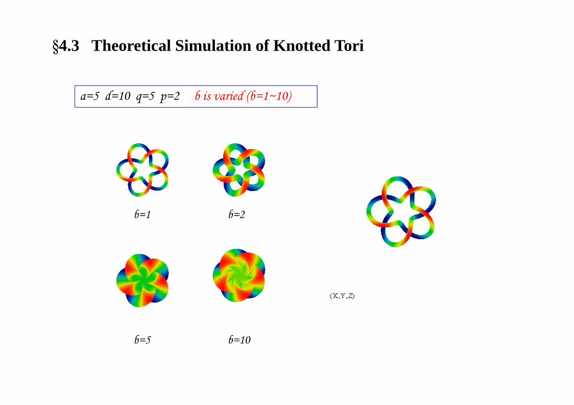
a=5 d=10 q=5 p=2 b is varied (b=1~10)
b=1 b=2
b=5 b=10
§4.3 Theoretical Simulation of Knotted Tori

)4,7()7,4(
Pattern (p,q) differs from pattern (q,p)
§4.4 Theoretical Simulation of Knotted Tori

b=2
b=5
§4.5 Different Visual Angle of Knotted Tori

LISSAJOUS KNOT ?

In knot theory, a Lissajous knot is a knot defined by parametric equations of theform :
§5.1 Mathematical Definition of Lissajous Knot
cos
cos
cos
x x
y y
z z
x n
y n
z n
where nx, ny, and nz are integers and the phase shifts φx, φy, and φz may be any real numbers.

§5.2 Reference Paper of Lissajous Knot

§5.3 Theoretical simulation of Various Lissajous Knot
cos
cos
cos
x
y
z
x n
y n
z n
, , 1, 1, 1x y zn n n 1, 2, 1
1, 1, 2 2, 1, 1
Observation from y-z plane :

§5.3 Theoretical simulation of Various Lissajous Knot
, , 1, 1, 3x y zn n n 1, 3, 5
1, 2, 3 1, 4, 5
1, 3, 4 1, 4, 9
Observation from y-z plane :

2-D Plot
, , 2, 3, 7
, , 0.2 , 0.7 , 0.7
x y z
x y z
n n n
X-Y Plane X-Z Plane Y-Z Plane
3-D Scatter Plot
§5.4 Different Visual Angle of (2,3,7) - Lissajous Knot

§5.5 Distinct Knot Type For Different Relative Phase
, , 2, 3, 7 , 0 .8x y z x y y xn n n n n
, 0.2 , 0.7x y , 0.4 ,x y


![FINITE TYPE INVARIANTS OF W-KNOTTED OBJECTS I: W-KNOTS … · to universal finite type invariants of parenthesized tangles [BN6]. And we’re optimistic, indeed we believe, that](https://img.pdfslide.net/doc/110x75/5e94e7fce119865c9009b9fa/finite-type-invariants-of-w-knotted-objects-i-w-knots-to-universal-inite-type.jpg)


![Las Curvas de Lissajous[1] Terminado](https://img.pdfslide.net/doc/110x75/5571fda84979599169999d82/las-curvas-de-lissajous1-terminado.jpg)