1

Scientific Reticence: a DRAFT Discussion 26 October 2017

James Hansen

I am writing Scientific Reticence and the Fate of Humanity in response to a query from the editor of Atmospheric Chemistry and Physics who handled Ice Melt, Sea Level Rise and Superstorms.1 That paper, together with Young People’s Burden,2 makes the case for a low global warming target and the urgency of phasing out fossil fuel emissions. We argue that global warming of 2°C, or even 1.5°C, is dangerous, because these levels are far above Holocene temperatures and even warmer than best estimates for the Eemian, when sea level reached 6-9 meters (20-30 feet) higher than today. Earth’s history shows that sea level adjusts to changes in global temperature. We conclude that eventual sea level rise of several meters could be locked in, if rapid emission reductions do not begin soon, and could occur within 50-150 years with the extraordinary climate forcing of continued “business-as-usual” fossil fuel emissions.

The editor noted that the Ice Melt paper was not highly cited or mainstream in climate impact discussions, and he was concerned because he thought it important for peer-reviewed extreme scenarios to be included in the upcoming IPCC AR6 cycle3. It might be added that both papers received VERY extensive peer review, all of which is available on the journals’ web sites.

I responded that I was not surprised by the minimal of citations. A public affairs person handling media contacts for the Ice Melt paper reported that a leading science reporter decided not to write about the paper, and later declined to write about the Burden paper, because 5 of the 6 experts he contacted advised against reporting on it. If the top people in a field are negative and do not cite a paper, it is license for others to ignore it, perhaps even a warning to younger researchers.

Scientific reticence may play a role here – I should be able to recognize that as well as anyone. However, my specific interpretation in terms of the famous elephant story is not as obvious. One would think that top experts in the field should have enough perspective to avoid that malady. Perhaps they even have a basis that should be presented for believing that a 2°C global warming limit provides a safe guardrail. It would be good to learn the basis for that in view of all the contrary evidence that we present in the two papers. Therefore I have written this Scientific Reticence piece as a DRAFT – also because I have not yet given my co-authors on the two papers a change to comment on it -- that I plan to revise after getting back from the Bonn COP.

1 Hansen, J., M. Sato, P. Hearty, R. Ruedy, M. Kelley, V. Masson-Delmotte, G. Russell, G. Tselioudis, J. Cao, E. Rignot, I. Velicogna, B. Tormey, B. Donovan, E. Kandiano, K. von Schuckmann, P. Kharecha, A.N. LeGrande, M. Bauer, and K. Lo: Ice melt, sea level rise and superstorms: Evidence from paleoclimate data, climate modeling, and modern observations that 2°C global warming could be dangerous. Atmos. Chem. Phys., 16, 3761-3812, 2016. 2 Hansen, J., M. Sato, P. Kharecha, K. von Schuckmann, D.J. Beerling, J. Cao, S. Marcott, V. Masson-Delmotte, M.J. Prather, E.J. Rohling, J. Shakun, P. Smith, A. Lacis, G. Russell, and R. Ruedy: Young people's burden: Requirement of negative CO2 emissions. Earth Syst. Dynam., 8, 577-616, doi:10.5194/esd-8-577-2017, 2017. 3 Intergovernmental Panel on Climate Change Sixth Assessment Report (https://wg1.ipcc.ch/AR6/AR6.html).

2

Scientific Reticence and the Fate of Humanity 26 October 2017

James Hansen

Frank Dentener, an editor of Atmospheric Chemistry and Physics, in a recent note to me observed that Ice Melt, Sea Level Rise, and Superstorms4, hereafter Ice Melt, was not highly cited or mainstream in climate impact discussions. He was concerned because he thought it important for peer-reviewed extreme scenarios to be included in the upcoming IPCC AR6 cycle5.

In Ice Melt, summarized in a video, we use paleoclimate analyses, climate modeling, and modern observations to expose a global climate emergency: fossil fuel emissions must be reduced as rapidly as practical. A proposed 2°C global warming target is not a safe “guardrail” – 2°C warming would lock in unconscionable climate impacts on young people and future generations. Earth’s present energy imbalance, with most of the excess energy pouring into the ocean, assures continued ocean warming for decades and threatens to lock in amplifying climate feedbacks, melting of ice shelves and nonlinearly growing sea level rise. Earth’s energy imbalance also assures continued long-term warming of land areas, with increasingly extreme droughts, floods and storms. Subtropics in summer and the tropics year-round are becoming uncomfortably warm; these areas will become less habitable if warming continues, increasing immigration pressures and global governance problems. Responsibility for these affairs will lie with the developed world. Our related Young People’s Burden6 paper shows that continued high fossil fuel emissions unarguably sentences young people to either a massive, implausible cleanup of atmospheric CO2 or growing deleterious impacts or both.

Below I examine whether recent observations support the conclusions in the Ice Melt paper.

First, however, I address “scientific reticence,” which I suspect affects consideration of our Ice Melt and Young People’s Burden papers – more important, it affects public understanding of climate change and the prospects for avoiding disastrous climate impacts. I once wrote about Scientific Reticence and Sea Level Rise7 from an academic perspective, concluding, in agreement with Eipper8, that scientists should not shrink from exercising their rights as citizens and responsibilities as scientists. Here it may be more informative if I describe two personal examples, papers I published in 19819 and 198810, each with many co-authors and each with receptions similar to that of the Ice Melt paper. Those two papers probably had the most impact

4 Hansen, J., M. Sato, P. Hearty, R. Ruedy, M. Kelley, V. Masson-Delmotte, G. Russell, G. Tselioudis, J. Cao, E. Rignot, I. Velicogna, B. Tormey, B. Donovan, E. Kandiano, K. von Schuckmann, P. Kharecha, A.N. LeGrande, M. Bauer, and K.-W. Lo: Ice melt, sea level rise and superstorms: Evidence from paleoclimate data, climate modeling, and modern observations that 2°C global warming could be dangerous. Atmos. Chem. Phys., 16, 3761-3812, 2016. 5 Intergovernmental Panel on Climate Change Sixth Assessment Report (https://wg1.ipcc.ch/AR6/AR6.html). 6 Hansen, J., M. Sato, P. Kharecha, K. von Schuckmann, D.J. Beerling, J. Cao, S. Marcott, V. Masson-Delmotte, M.J. Prather, E.J. Rohling, J. Shakun, P. Smith, A. Lacis, G. Russell, and R. Ruedy: Young people's burden: Requirement of negative CO2 emissions. Earth Syst. Dynam., 8, 577-616, 2017. 7 Hansen, J.E.: Scientific reticence and sea level rise. Environ. Res. Lett., 2, 024002, 2007. 8 Eipper, A.W.: Pollution problems, resource policy, and the scientist, Science, 169, 11-15, 1970. 9 Hansen, J., D. Johnson, A. Lacis, S. Lebedeff, P. Lee, D. Rind, and G. Russell: Climate impact of increasing atmospheric carbon dioxide. Science, 213, 957-966, doi:10.1126/science.213.4511.957, 1981 10 Hansen, J., I. Fung, A. Lacis, D. Rind, S. Lebedeff, R. Ruedy, G. Russell, and P. Stone: Global climate changes as forecast by Goddard Institute for Space Studies three-dimensional model. J. Geophys. Res., 93, 9341-9364, 1988.

3

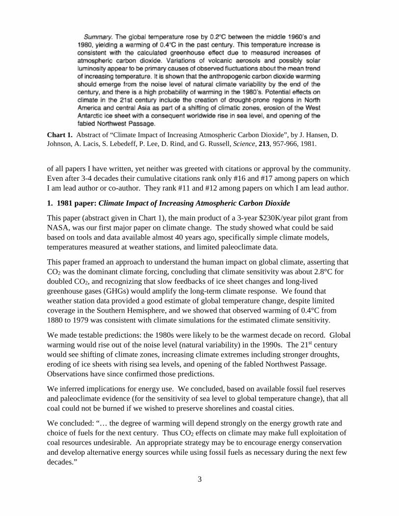
Chart 1. Abstract of “Climate Impact of Increasing Atmospheric Carbon Dioxide”, by J. Hansen, D. Johnson, A. Lacis, S. Lebedeff, P. Lee, D. Rind, and G. Russell, Science, 213, 957-966, 1981.

of all papers I have written, yet neither was greeted with citations or approval by the community. Even after 3-4 decades their cumulative citations rank only #16 and #17 among papers on which I am lead author or co-author. They rank #11 and #12 among papers on which I am lead author.

1. 1981 paper: Climate Impact of Increasing Atmospheric Carbon Dioxide

This paper (abstract given in Chart 1), the main product of a 3-year $230K/year pilot grant from NASA, was our first major paper on climate change. The study showed what could be said based on tools and data available almost 40 years ago, specifically simple climate models, temperatures measured at weather stations, and limited paleoclimate data.

This paper framed an approach to understand the human impact on global climate, asserting that CO2 was the dominant climate forcing, concluding that climate sensitivity was about 2.8°C for doubled CO2, and recognizing that slow feedbacks of ice sheet changes and long-lived greenhouse gases (GHGs) would amplify the long-term climate response. We found that weather station data provided a good estimate of global temperature change, despite limited coverage in the Southern Hemisphere, and we showed that observed warming of 0.4°C from 1880 to 1979 was consistent with climate simulations for the estimated climate sensitivity.

We made testable predictions: the 1980s were likely to be the warmest decade on record. Global warming would rise out of the noise level (natural variability) in the 1990s. The 21st century would see shifting of climate zones, increasing climate extremes including stronger droughts, eroding of ice sheets with rising sea levels, and opening of the fabled Northwest Passage. Observations have since confirmed those predictions.

We inferred implications for energy use. We concluded, based on available fossil fuel reserves and paleoclimate evidence (for the sensitivity of sea level to global temperature change), that all coal could not be burned if we wished to preserve shorelines and coastal cities.

We concluded: “… the degree of warming will depend strongly on the energy growth rate and choice of fuels for the next century. Thus CO2 effects on climate may make full exploitation of coal resources undesirable. An appropriate strategy may be to encourage energy conservation and develop alternative energy sources while using fossil fuels as necessary during the next few decades.”

4

This paper in Science received widespread attention, including, front page reporting in the New York Times and lead editorials in the Washington Post and New York Times. The paper also led to my first testimony to Congress, to a Joint Hearing of two House of Representatives Subcommittees on Carbon Dioxide and the Greenhouse Effect on 25 March 1982.

Scientific criticism and commentary, appropriate for any paper that is pushing the boundaries, was abundant and largely reasonable. Walter Sullivan, the exceptional science writer for the New York Times, listed a large number of uncertainties noted by Steve Schneider and then dryly stated “These uncertainties are, to a large extent, recognized in the new report, signed by Dr. James Hansen and six colleagues at the space studies institute.”11

Criticisms submitted to journals and eventually published included one by S.I. Rasool12 that lists a large number of uncertainties and then asks, given those, how can we make any prediction of climate change? The short answer is to recognize the forest for the trees, specifically to realize that CO2 is the dominant climate forcing, that we have sound estimates of global climate sensitivity, and there is substantial offset among the weaker forcings.

But Rasool provided his own answer9: “I guess the answer lies in the fact that some of us feel compelled to emphasize the worst case in order to get the attention of decision makers who control the funding.” Our response13 was: “As scientists we did our best to present an unbiased projection of likely climatic effects of CO2. We also fulfilled what we believe is a responsibility of scientists: to point out clearly the consequences of their findings.”

Less ad hominem criticism was published in Science14, but it also failed to distinguish the big picture from details. This published criticism also asserted that temperature observations contradicted the principal sub-global prediction of climate models: that temperature changes should be magnified in polar regions. In fact, as we showed in our response,15 the data confirm the predicted enhancement of Arctic warming over the global mean. Nevertheless, these criticisms were cited by Department of Energy (DoE) program managers, who decided to renege on their promise to continue the $230K/year funding for our CO2/climate research program when responsibility for the CO2/climate program was assigned to DoE.

Funding decisions for other researchers, I noted, sent a clear message: funding prospects were brighter if one emphasized that the science was very uncertain and that much more research was needed before it might be possible to draw inferences related to policy. Concern about policy implications varies depending upon which political party is in power, but desire to avoid this landmine is one of several factors that encourage scientific reticence.4

Events related to our 1988 paper (citation rank #16), and congressional testimony based on that paper, provide even clearer empirical evidence for scientific reticence about climate change.

11 Sullivan, W.: Study finds warming trend that could raise sea levels, New York Times, 22 August 1981. 12 Rasool, S.I.: On predicting calamities, Clim. Change, 5, 201-202, 1983. 13 Hansen, J., et al.: Response to “On predicting calamities”, Clim. Change, 5, 201-202, 1983. 14 MacCracken, M.C.: Climatic effects of atmospheric carbon dioxide, Science, 220, 873-874, 1983. 15 Hansen, J., et al.: Response to MacCracken and Idso, Science, 220, 874-875, 1983.

5

2. 1988 paper: Global Climate Changes as Forecast by Goddard Institute for Space Studies Three-Dimensional Model6

This paper provided much of the basis for testimony I gave to the U. S. Senate on 23 June 1988. My conclusion that greenhouse gases were already having a significant effect on global climate did not meet with universal acclamation. The reaction was captured well by Richard Kerr’s article Hansen vs. the World on the Greenhouse Threat,16 as I will discuss.

By 1988 we had temperature data for almost one additional decade beyond the data used for our 1981 paper, which used temperature data through 1978. By 1988 we had set up near-real-time data processing, updating the global temperature record every month. The data revealed that the 1980s would easily be the warmest decade in the period of instrumental data that began in 1880, confirming one of the predictions in the 1981 paper. Also the first five months of 1988 were so warm that I could state that 1988 was likely to be the single warmest year in the entire record.

By 1988 my colleagues at the Goddard Institute and I also had completed a study Climate Sensitivity: Analysis of Feedback Mechanisms17 that illuminated the roles of fast and slow feedback processes in determining climate sensitivity and climate response time. The paleo analysis confirmed the high climate sensitivity obtained in models incorporating only fast feedbacks, and it showed that slow feedbacks further amplify long-term climate response.18

By 1988 atmospheric CO2 had reached 350 ppm, at least 25 percent above its preindustrial level. And other GHGs, especially CH4, N2O, and chlorofluorocarbons were adding almost as much radiative forcing as CO2

19 making the GHG radiative forcing equivalent to almost 400 ppm CO2.

This human-made change, most of it achieved within the preceding few decades, was as great as that associated with the climate change from a deep ice age to an interglacial warm period.

To understand the implications of these facts we must use all the tools in our toolbox. Important tools include (1) insights based on knowledge of Earth’s climate history, (2) climate models, and (3) observations of climate change during the modern era of instrumental measurements.

16 Kerr, R.A.: Hansen vs. the world on the greenhouse threat, Science, 244, 1041-1043, 1989. 17 Hansen, J., A. Lacis, D. Rind, G. Russell, P. Stone, I. Fung, R. Ruedy, and J. Lerner: Climate sensitivity: Analysis of feedback mechanisms. In Climate Processes and Climate Sensitivity. J.E. Hansen and T. Takahashi, Eds., AGU Geophysical Monograph 29, Maurice Ewing Volume 5. American Geophysical Union, 130-163, 1984. 18 We compared the last glacial maximum (LGM, the period about 20,000 years ago when a large ice sheet covered Canada and parts of the United States) with the present interglacial period. We could use data for these two periods to find an accurate empirical measure of the fast-feedback climate sensitivity, which is the climate sensitivity relevant to decade-century time scales, by taking ice sheet size and long-lived GHG amounts as specified boundary conditions in both periods. However, on longer time scales ice sheet size and CO2 amount are slow amplifying feedbacks, which accounts for the extraordinarily high climate sensitivity on millennial time scales. The high sensitivity on millennial time scales is the reason that small climate forcings caused by perturbations of Earth’s orbit and the tilt of Earth’s spin axis cause large glacial-to-interglacial climate oscillations. 19 Lacis, A., J. Hansen, P. Lee, T. Mitchell, and S. Lebedeff: Greenhouse effect of trace gases, 1970-1980. Geophys. Res. Lett., 8, 1035-1038, doi:10.1029/GL008i010p01035, 1981.

6

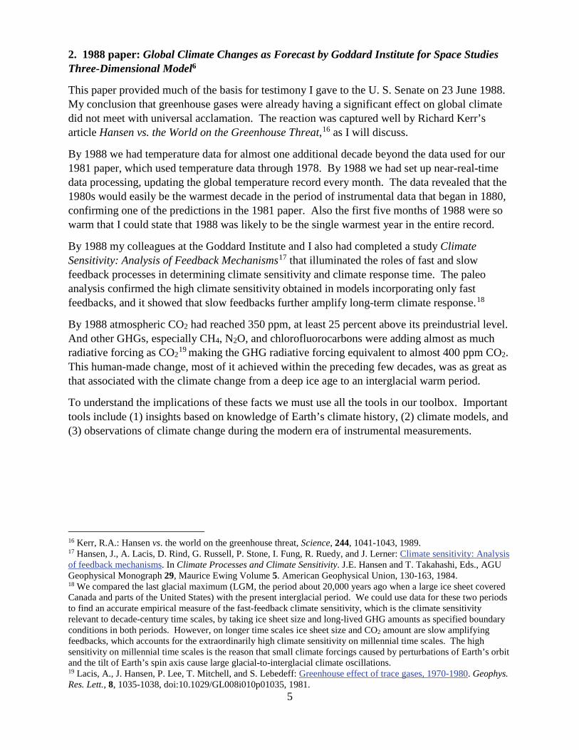
Chart 2. (a) Greenhouse gas scenarios in 1988 GCM simulations, (b) Observed temperature compared with simulations for scenarios A, B, C. Shaded range was based on estimated global temperature at peaks of the current and prior interglacial periods, about 6,000 and 120,000 years ago.

Kerr’s Hansen vs. the World article illustrates what I mean. A mathematician looks at a series of global temperatures and concludes that they do not prove human-made warming with high confidence. A climate modeler says many processes in the models are not simulated well, so results are unreliable. They are correct that conclusions based on a single approach are limited. However, it is like the proverbial blind-folded men, each feeling a different part of the elephant. No one of them, by himself, can determine the nature of the beast. If they pooled their data they might figure it out, but the committee approach is a tortuous process. Success is limited by the weakest member, and the process is slow. That is why you cannot do good multidisciplinary science simply by putting scientists from different disciplines into the same building. You do good science by putting the information from multiple disciplines into the same brain.

I am not saying that I was the only one who understood in the late 1980s that the world was getting warmer because of the extraordinary human-caused change of atmospheric composition. On the contrary, one of the scientists interviewed by Kerr said “if there were a secret ballot at this meeting on the question, most people would say that the greenhouse warming is probably there.” Another said “What bothers a lot of us is that we have a scientist telling Congress things that we are reluctant to say ourselves.”

That is scientific reticence. It needs to be understood, because the same thing is happening now. But now the stakes are much higher, and the urgency of cutting through reticence is greater.

However, before describing today’s situation, let’s try to learn something from the 1988 paper. Predictions in our 1981 paper proved to be accurate, but what about the 1988 climate paper?

We made calculations with a 3-D global climate model (GCM) including a simple representation of the ocean with diffusive mixing of heat anomalies into the deep ocean and specified horizontal ocean heat transport. The model had coarse spatial resolution, because of our limited computer resources.20 The GCM climate simulations in the 1988 paper had horizontal resolution 4 degrees

20 A few months after I was appointed as Director of the Goddard Institute for Space Studies in 1981, I received direction from management of the parent Goddard Space Flight Center (GSFC) to make preparations to move the Institute to the main campus in Greenbelt, Maryland. After getting support of a few key staff members, I told the GSFC Director that they would only get used government furniture – none of us were going. We were allowed to stay near the Columbia University campus, but the GSFC Director told me that we could never expect much

7

latitude and 5 degrees longitude, coarse enough that we could complete simulations for 1958-2020 for three GHG scenarios in about one-year, running the model as the background job on the computer so that it soaked up all available time, mainly overnight and weekends.

We made climate simulations for three GHG scenarios: (A) continued rapid growth of the annual increment of GHGs, similar to growth from 1950 to early 1980s, (B) constant annual increment of GHGs, (C) stabilization of atmospheric GHG amounts beginning in 2000. We suggested that scenario B, with approximately constant annual increases of the GHG climate forcing, was the most plausible, with scenarios A and C marking an extreme range of possibilities.21 Real world GHG climate forcing turned out to be very close to scenario B (Chart 2a).22

Observed global temperature increased after 1988, rising far out of the natural variability range. Global temperature is now far above the warmest preindustrial time in the Holocene (the current interglacial period, now more than 10,000 years long, during which civilization developed) and approximately matches the peak temperature of the Eemian period (about 120,000 years ago).3 The real world warmed somewhat slower than the model reaching temperature anomaly +1°C about 5 years later than the model. The greater warming in the model is well accounted for by the fact that the model’s sensitivity was 4.2°C for 2×CO2 (i.e., for doubled CO2, which is a forcing of 4 W/m2), while paleoclimate data and known climate feedbacks suggest that actual (fast feedback) climate sensitivity is close to 3°C for 2×CO2. We understood that the model’s sensitivity was near the upper end of the accepted range (3±1.5°C for 2×CO2), but unlike the 1-D model used in our 1981 paper, we could not simply adjust the sensitivity to match best knowledge of climate sensitivity.23 We could only afford one set of model runs with this first version of our 3-D model, but in interpreting the model runs we can bear in mind the model’s high sensitivity. Subsequent simulations with newer versions of our model with sensitivity near 3°C for 2×CO2 and simulations by dozens of other modeling groups reported by IPCC24 confirm good agreement of modeled and observed global temperature change.

resources if we remained remote. Fortunately, we were able to use money saved by cancelling the maintenance contract on our IBM 360-95 (1967 vintage) to purchase a used Amdahl (1975 vintage). The latter was a bit faster than the old IBM, reliable, and low maintenance. By the middle and late 1980s our computer capacity was a factor of 10 to 100 less than that of the other major modeling groups, but we had the advantage of an academic environment away from the growing NASA bureaucracy. 21 Scenario A had rapid growth of annual GHG emissions, as occurred in 1950-1980 (see Fig. 8 of Young People’s Burden3). Scenario C assumed 21st century GHG emissions would decrease to a level just balancing GHG sinks. 22 The annual growth of GHG forcing increased rapidly from ~0.02 W/m2 per year in 1958 to ~0.045 W/m2 per year in the early 1980s; it then fell to ~0.035 W/m2, remaining at that level until the past five years when it increased sharply to ~0.045 W/m2 per year, belying a misperception that the corner has been turned on the global warming problem (see Figs. 8 and 14 in Young People’s Burden3). 23 The high model sensitivity was later traced to an excessive amplifying cloud feedback. Next most important model deficiencies were (a) unchanging tropospheric aerosols, and (b) assumption of energy balance when the simulation was initiated, i.e., in 1958. These approximations affected global temperature in opposite senses and were thus at least partially offsetting. 24 IPCC (Intergovernmental Panel on Climate Change): Climate Change 2013, edited by: Stocker, T., Qin, D., Q., Plattner, G. K., Tignor, M. M. B., Allen, S. K., Boschung, J., Nauels, A., Xia, Y., Bex, V., and Midgley, P. M., Cambridge University Press, 1535 pp., 2013.

8

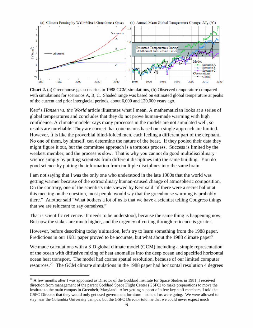
Chart 3. Surface air temperature (°C) simulated with rapidly increasing GHGs and rapidly increasing freshwater discharge from Greenland and Antarctica (Fig. 16 of reference 1).

3. Ice Melt paper

In 2007-8 we made climate simulations driven by GHG scenario25 A1B plus rapidly growing ice and fresh water discharge from Antarctica and Greenland. The 4°×5° climate model found cooling southeast of Greenland and around Antarctica associated with reduced deep water formation in the North Atlantic and reduced bottom water formation around Antarctica. We traced surface cooling and reduced ocean overturning in part to cooling from melting ice but mainly to the buoyancy effect of the added fresh water in upper ocean layers.

As discussed in Section 2 (Background Information) of our Ice Melt paper, I was interested in the potential relation of these effects to evidence that Paul Hearty found for rapid sea level rise and North Atlantic storminess late in the Eemian interglacial period. These initial simulations affected interpretations in my book, Storms of My Grandchildren,26 but we did not begin to write a paper on the climate simulations until several years later, by which time improvements had been made in the ocean model, as described in Section 3 of the Ice Melt paper.

Thus we repeated the fresh water discharge experiments with the newer model, again finding surface cooling (Chart 3) and subsurface ocean warming similar to that in the older model. The subsurface warming occurs at depths where it can melt the underside of ice shelves, the tongues of ice extending from ice sheets into the ocean, especially at the depths of their grounding lines. This subsurface warming helps explain ice shelf retreat, ice sheet disintegration and sea level rise in paleoclimate data (Shaffer et al., 200427; Petersen et al., 201328).

25 A1B, a “business-as-usual” scenario in earlier IPCC reports, falls between recent RCP8.5 and RCP6.0 scenarios. 26 Hansen, J.: Storms of My Grandchildren, New York, Bloomsbury, 304 pp., 2009. 27 Shaffer, G., Olsen, S.M., and Bjerrum, C.J.: Ocean subsurface warming as a mechanism for coupling Dansgaard-Oeschger climate cycles and ice-rafting events, Geophys. Res. Lett., 31(24), L24202, 2004. 28 Petersen, S.V., Schrag, D.P., and Clark, P.U.: A new mechanism for Dansgaard-Oeschger cycles, Paleoceanography, 28, 24-30, 2013.

9

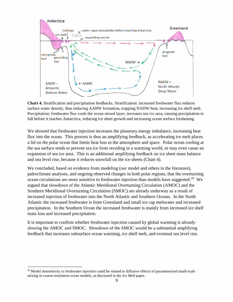
Chart 4. Stratification and precipitation feedbacks. Stratification: increased freshwater flux reduces surface water density, thus reducing AABW formation, trapping NADW heat, increasing ice shelf melt. Precipitation: freshwater flux cools the ocean mixed layer, increases sea ice area, causing precipitation to fall before it reaches Antarctica, reducing ice sheet growth and increasing ocean surface freshening.

We showed that freshwater injection increases the planetary energy imbalance, increasing heat flux into the ocean. This process is thus an amplifying feedback, as accelerating ice melt places a lid on the polar ocean that limits heat loss to the atmosphere and space. Polar ocean cooling at the sea surface tends to prevent sea ice from receding in a warming world, or may even cause an expansion of sea ice area. This is an additional amplifying feedback on ice sheet mass balance and sea level rise, because it reduces snowfall on the ice sheets (Chart 4).

We concluded, based on evidence from modeling (our model and others in the literature), paleoclimate analyses, and ongoing observed changes in both polar regions, that the overturning ocean circulations are more sensitive to freshwater injection than models have suggested.29 We argued that slowdown of the Atlantic Meridional Overturning Circulation (AMOC) and the Southern Meridional Overturning Circulation (SMOC) are already underway as a result of increased injection of freshwater into the North Atlantic and Southern Oceans. In the North Atlantic the increased freshwater is from Greenland and small ice cap meltwater and increased precipitation. In the Southern Ocean the increased freshwater is mainly from increased ice shelf mass loss and increased precipitation.

It is important to confirm whether freshwater injection caused by global warming is already slowing the AMOC and SMOC. Slowdown of the SMOC would be a substantial amplifying feedback that increases subsurface ocean warming, ice shelf melt, and eventual sea level rise.

29 Model insensitivity to freshwater injection could be related to diffusive effects of parameterized small-scale mixing in coarse-resolution ocean models, as discussed in the Ice Melt paper.

10

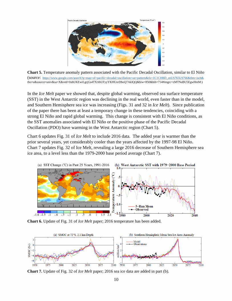
Chart 5. Temperature anomaly pattern associated with the Pacific Decadal Oscillation, similar to El Niño (source: https://www.google.com/search?q=map+of+pacific+decadal+oscillation+sst+pattern&rlz=1C1CHBD_enUS765US766&tbm=isch& tbo=u&source=univ&sa=X&ved=0ahUKEwiLgrjGs4TXAhUFyyYKHUorDboQ7AkIQQ&biw=850&bih=714#imgrc=zMTNaBU5EgwHmM:)

In the Ice Melt paper we showed that, despite global warming, observed sea surface temperature (SST) in the West Antarctic region was declining in the real world, even faster than in the model, and Southern Hemisphere sea ice was increasing (Figs. 31 and 32 in Ice Melt). Since publication of the paper there has been at least a temporary change in these tendencies, coinciding with a strong El Niño and rapid global warming. This change is consistent with El Niño conditions, as the SST anomalies associated with El Niño or the positive phase of the Pacific Decadal Oscillation (PDO) have warming in the West Antarctic region (Chart 5).

Chart 6 updates Fig. 31 of Ice Melt to include 2016 data. The added year is warmer than the prior several years, yet considerably cooler than the years affected by the 1997-98 El Niño. Chart 7 updates Fig. 32 of Ice Melt, revealing a large 2016 decrease of Southern Hemisphere sea ice area, to a level less than the 1979-2000 base period average (Chart 7).

Chart 6. Update of Fig. 31 of Ice Melt paper; 2016 temperature has been added.

Chart 7. Update of Fig. 32 of Ice Melt paper; 2016 sea ice data are added in part (b).

11

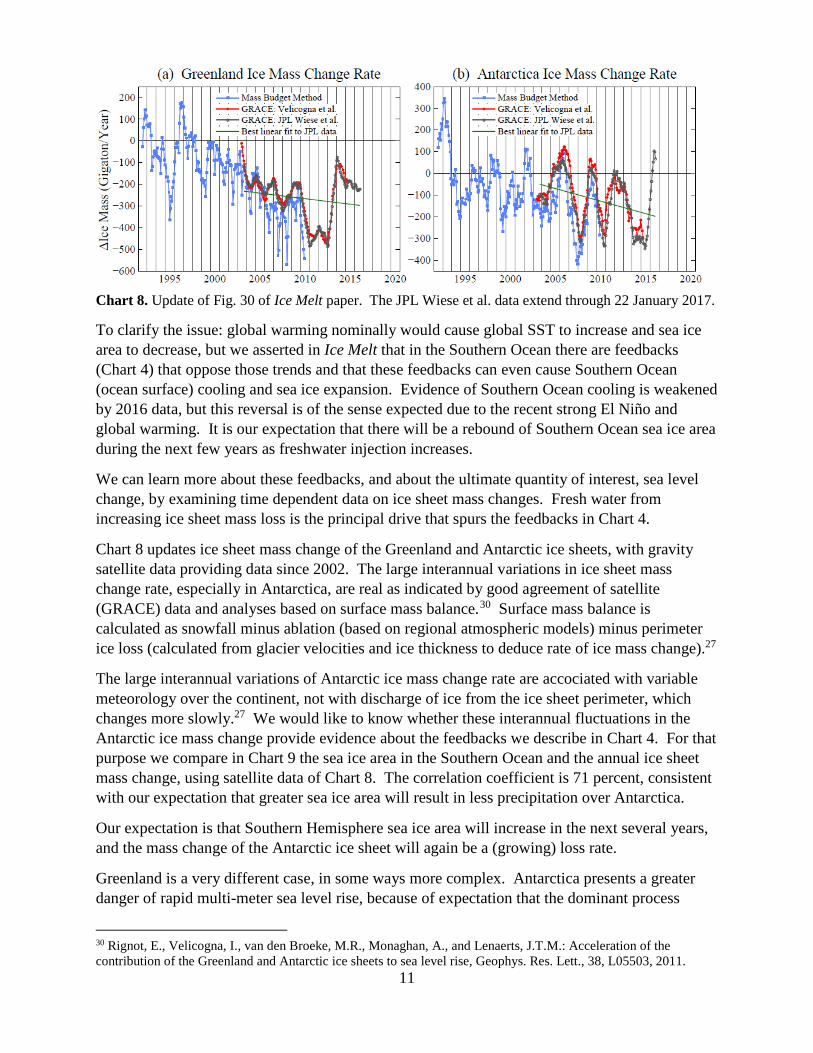
Chart 8. Update of Fig. 30 of Ice Melt paper. The JPL Wiese et al. data extend through 22 January 2017.

To clarify the issue: global warming nominally would cause global SST to increase and sea ice area to decrease, but we asserted in Ice Melt that in the Southern Ocean there are feedbacks (Chart 4) that oppose those trends and that these feedbacks can even cause Southern Ocean (ocean surface) cooling and sea ice expansion. Evidence of Southern Ocean cooling is weakened by 2016 data, but this reversal is of the sense expected due to the recent strong El Niño and global warming. It is our expectation that there will be a rebound of Southern Ocean sea ice area during the next few years as freshwater injection increases.

We can learn more about these feedbacks, and about the ultimate quantity of interest, sea level change, by examining time dependent data on ice sheet mass changes. Fresh water from increasing ice sheet mass loss is the principal drive that spurs the feedbacks in Chart 4.

Chart 8 updates ice sheet mass change of the Greenland and Antarctic ice sheets, with gravity satellite data providing data since 2002. The large interannual variations in ice sheet mass change rate, especially in Antarctica, are real as indicated by good agreement of satellite (GRACE) data and analyses based on surface mass balance.30 Surface mass balance is calculated as snowfall minus ablation (based on regional atmospheric models) minus perimeter ice loss (calculated from glacier velocities and ice thickness to deduce rate of ice mass change).27

The large interannual variations of Antarctic ice mass change rate are accociated with variable meteorology over the continent, not with discharge of ice from the ice sheet perimeter, which changes more slowly.27 We would like to know whether these interannual fluctuations in the Antarctic ice mass change provide evidence about the feedbacks we describe in Chart 4. For that purpose we compare in Chart 9 the sea ice area in the Southern Ocean and the annual ice sheet mass change, using satellite data of Chart 8. The correlation coefficient is 71 percent, consistent with our expectation that greater sea ice area will result in less precipitation over Antarctica.

Our expectation is that Southern Hemisphere sea ice area will increase in the next several years, and the mass change of the Antarctic ice sheet will again be a (growing) loss rate.

Greenland is a very different case, in some ways more complex. Antarctica presents a greater danger of rapid multi-meter sea level rise, because of expectation that the dominant process

30 Rignot, E., Velicogna, I., van den Broeke, M.R., Monaghan, A., and Lenaerts, J.T.M.: Acceleration of the contribution of the Greenland and Antarctic ice sheets to sea level rise, Geophys. Res. Lett., 38, L05503, 2011.

12

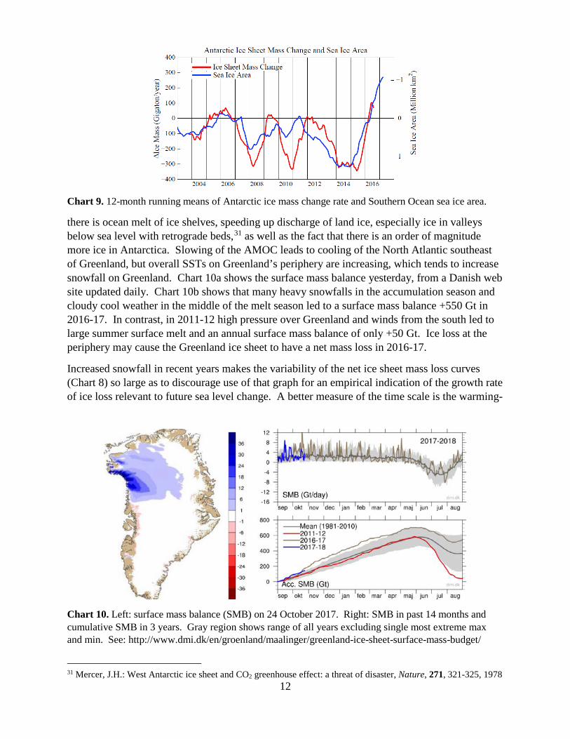
Chart 9. 12-month running means of Antarctic ice mass change rate and Southern Ocean sea ice area.

there is ocean melt of ice shelves, speeding up discharge of land ice, especially ice in valleys below sea level with retrograde beds,31 as well as the fact that there is an order of magnitude more ice in Antarctica. Slowing of the AMOC leads to cooling of the North Atlantic southeast of Greenland, but overall SSTs on Greenland’s periphery are increasing, which tends to increase snowfall on Greenland. Chart 10a shows the surface mass balance yesterday, from a Danish web site updated daily. Chart 10b shows that many heavy snowfalls in the accumulation season and cloudy cool weather in the middle of the melt season led to a surface mass balance +550 Gt in 2016-17. In contrast, in 2011-12 high pressure over Greenland and winds from the south led to large summer surface melt and an annual surface mass balance of only +50 Gt. Ice loss at the periphery may cause the Greenland ice sheet to have a net mass loss in 2016-17.

Increased snowfall in recent years makes the variability of the net ice sheet mass loss curves (Chart 8) so large as to discourage use of that graph for an empirical indication of the growth rate of ice loss relevant to future sea level change. A better measure of the time scale is the warming-

Chart 10. Left: surface mass balance (SMB) on 24 October 2017. Right: SMB in past 14 months and cumulative SMB in 3 years. Gray region shows range of all years excluding single most extreme max and min. See: http://www.dmi.dk/en/groenland/maalinger/greenland-ice-sheet-surface-mass-budget/

31 Mercer, J.H.: West Antarctic ice sheet and CO2 greenhouse effect: a threat of disaster, Nature, 271, 321-325, 1978

13

induced increase in the discharge rate of land-based ice from the ice sheet perimeter, because that is the quantity that will eventually determine the time scale for sea level rise. This increment to the peripheral ice discharge rate can be obtained as the difference between the satellite-measured ice sheet mass change and the surface mass balance as defined in Chart 10. If this increment to the peripheral ice discharge rate has a doubling time as short as 10-20 years, multi-meter sea level rise can be expected in 50-150 years, as concluded in our Ice Melt paper for the case of business-as-usual fossil fuel emissions continue (A1B scenario). More on this topic later.

4. Young People’s Burden paper3

In Burden we show that present global temperature is already far above its range during the preindustrial Holocene, i.e., above the levels that existed during the period in which civilization developed. Indeed, the present global temperature has reached the peak level during the Eemian, the prior interglacial period when sea level reached 6-9 m (20-30 feet) higher than today.

The rapidity of ice sheet and sea level response to global temperature is difficult to predict, but it depends on the magnitude of warming. Targets for limiting global warming, at minimum, must aim to avoid leaving global temperature at Eemian or higher levels for centuries. Such targets now require “negative emissions”, i.e., extraction of CO2 from the air.

If phasedown of fossil fuel emissions begins soon, improved agricultural and forestry practices, including reforestation and steps to improve soil fertility and increase its carbon content, may provide much of the necessary CO2 extraction. In that case, the magnitude and duration of global temperature excursion above the natural range of the current interglacial (Holocene) could be limited and irreversible climate impacts could be minimized.

In contrast, continued high fossil fuel emissions will place a burden on young people to undertake massive technological CO2 extraction if they are to limit climate change and its consequences. Proposed methods of extraction such as bioenergy with carbon capture and storage (BECCS) or air capture of CO2 have minimal estimated costs of 89-535 trillion dollars this century and also have large risks and uncertain feasibility.

We conclude that continued high fossil fuel emissions unarguably sentences young people to either a massive, implausible cleanup or growing deleterious climate impacts or both.

The Paris Agreement,32 slowdown of the growth rate of fossil fuel CO2 emissions, and falling prices of renewable energies have contributed to a widespread optimism about progress toward stabilizing climate. In Burden we show that real world data do not support that optimism.

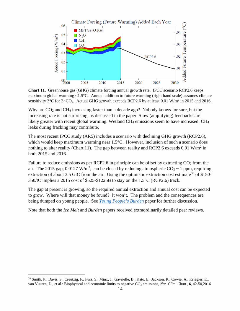
Chart 11 shows the annual increase of greenhouse gas climate forcing. The annual change is growing, not decreasing! That growth continues up to the present. The figure appears to go only through 2015, because we smooth data to minimize effects of short-term variability, mainly the Southern Oscillation. The figure is from the EGU video on the Young People’s Burden paper, for which observations of atmospheric gas amounts are updated monthly on our website.

32 Paris Agreement, UNFCCC secretariat, available at http://unfccc.int/paris_agreement/items/9485.php, 2015.

14

Chart 11. Greenhouse gas (GHG) climate forcing annual growth rate. IPCC scenario RCP2.6 keeps maximum global warming <1.5°C. Annual addition to future warming (right hand scale) assumes climate sensitivity 3°C for 2×CO2. Actual GHG growth exceeds RCP2.6 by at least 0.01 W/m2 in 2015 and 2016.

Why are CO2 and CH4 increasing faster than a decade ago? Nobody knows for sure, but the increasing rate is not surprising, as discussed in the paper. Slow (amplifying) feedbacks are likely greater with recent global warming. Wetland CH4 emissions seem to have increased; CH4 leaks during fracking may contribute.

The most recent IPCC study (AR5) includes a scenario with declining GHG growth (RCP2.6), which would keep maximum warming near 1.5°C. However, inclusion of such a scenario does nothing to alter reality (Chart 11). The gap between reality and RCP2.6 exceeds 0.01 W/m2 in both 2015 and 2016.

Failure to reduce emissions as per RCP2.6 in principle can be offset by extracting CO2 from the air. The 2015 gap, 0.0127 W/m2, can be closed by reducing atmospheric CO2 ~ 1 ppm, requiring extraction of about 3.5 GtC from the air. Using the optimistic extraction cost estimate33 of $150-350/tC implies a 2015 cost of $525-$1225B to stay on the 1.5°C (RCP2.6) track.

The gap at present is growing, so the required annual extraction and annual cost can be expected to grow. Where will that money be found? It won’t. The problem and the consequences are being dumped on young people. See Young People’s Burden paper for further discussion.

Note that both the Ice Melt and Burden papers received extraordinarily detailed peer reviews.

33 Smith, P., Davis, S., Creutzig, F., Fuss, S., Minx, J., Gavrielle, B., Kato, E., Jackson, R., Cowie, A., Kriegler, E., van Vuuren, D., et al.: Biophysical and economic limits to negative CO2 emissions, Nat. Clim. Chan., 6, 42-50,2016.

15

5. Discussion: Reticence?

It is conceivable that scientific reticence plays a part in the reactions to our papers, but I am not convinced that it is the whole story. In the 1981 and 1988/89 examples discussed above there was evidence, in the reviews of those papers and in the published commentaries, that much of the criticism suffered from the “blindfolds and elephant” explanation. They did not seem to be considering the entirety of information that we had from paleoclimate, modern observations, and models, with recognition of model weaknesses. However, in current analyses it seems unlikely that recognized experts are not considering the full range of available information.

The Ice Melt paper is long. One author who does cite Ice Melt immediately dismisses it, because, he claims, the freshwater injection rates (hosing rates, he calls them) are unrealistically large. Obviously he did not read the paper. The injection/hosing rates are based on observed data for recent years and projected forward with different time scales for their growth rate (10, 20, 40 year doubling times). Our conclusion that the AMOC and SMOC are already beginning to slow down is based on current observations and model results in the present and near-term, not on the high rates of freshwater injection that occur after many doublings. When one such author rejects a paper based on such a misinterpretation, it is easy for the attitude to spread.

Criticism of IPCC. I chose in 1989, when faced with scientific reticence and more, to bail out of the media circus and focus only on science. When I reentered the fray in 2004 it was not just to criticize the lack of climate actions by the Bush Administration, but also to draw attention to the need for a low target on global warming if “dangerous” consequences were to be avoided. Specifically, as spelled out in A Slippery Slope,34 I criticized the sea level change analysis in the most recent (2001) IPCC report. IPCC scenarios had GHG amounts and calculated global temperatures that were “off the charts” compared to paleoclimate data covering hundreds of thousands or even millions of years, yet the calculations for the contribution of Greenland and Antarctica to sea level rise was measured in cm, very few cm. That didn’t seem plausible, as I argued on heuristic grounds, mainly concerned with the role of a warming ocean on ice shelves.

This came across as a criticism of IPCC. I cited Richard Feynmann insights in Slippery Slope, and more directly in Storms of My Grandchildren,35 about how the community tends to move slowly in correcting an error. He is talking about scientific reticence. However, I probably could have been more discrete in criticizing IPCC – after all, the scientists contributing to those long reports put in a lot of work for very little recognition.

Superstorms and flying boulders. Several reviews and commentaries seemed angry about the use of the word “superstorms” in the title, even asserting that it was intended to draw public attention to the paper. Duh. What a bad thing to do! Is this feeling related to scientific reticence?

We were not helped by the Washington Post article referring to flying boulders. We did not say that any boulders flew. Our interpretation of the boulders on Eleuthera is that powerful storm-driven late-Eemian waves, when sea level was several meters higher than today, transported the boulders from the cliffs below to their present location where they rest on Eemian substrate.

34 Hansen, J.E.: A slippery slope: How much global warming constitutes "dangerous anthropogenic interference"? An editorial essay. Clim. Change 68, 269-279, doi:10.1007/s10584-005-4135-0, 2005. 35 Hansen, J.: Storms of My Grandchildren, New York, Bloomsbury, 304 pp., 2009.

16

Recent publications have confirmed that storms can move very large boulders. The funneling nature of the bay on Eleuthera increases the power of the waves in the vicinity of the boulders. Boulders in that region moved during the Holocene are smaller, suggesting that some storms in the late Eemian were stronger than today.

None of the major conclusions in our paper, about the threat of large sea level rise or about AMOC and SMOC already slowing down, depend on interpretation of the Eleuthera boulders. However, I would like to draw attention to a new comprehensive review paper by Hearty and Tormey36 on the geologic evidence.

Early Discussion of Discussion paper and peer-review. Both the Ice Melt and Burden papers were submitted to journals that include publication of an initial “Discussion” version of the paper, after it has been checked and approved by an editor. This publication mode seemed especially appropriate for both papers: there were upcoming United Nations climate conferences and we hoped to get feedback from both scientists on the science and from the public and policymakers on the papers’ policy implications. However, there was criticism of whether the papers should be discussed publicly before the peer-review process is complete.

Even if there is merit to that position – and I see nothing wrong with presenting a discussion paper for discussion (!) as long as it is so identified – both papers subsequently passed detailed peer-review. Indeed, the Ice Melt paper seemed to go through further review by an editorial board, which seemed to redefine the word “dangerous” to mean something different than what the public means. See Dangerous Scientific Reticence.

Negative Emissions. Perhaps nothing illustrates the dangers of scientific reticence better than the way negative emissions crept into IPCC scenarios. Clarifying the implausibility of that scenario is an objective of our Burden paper.

Co-authors. People suggesting that we are exaggerating the global warming threat should take a close look at the list of co-authors. They include top scientists in the world in the relevant disciplines. I am grateful to them for all that they have done to help produce the two papers.

I note that I am sending out this draft discussion without showing it to the co-authors, because I need the next week to prepare materials for discussions at the Bonn COP meeting.

In an attempt to make up for any flaws in this draft, I include here a few cartoons to lighten the mood – even God and Noah have a sense of humor. Any suggestions re this reticence topic would be most welcome.

36 Hearty, P.J. and Tormey, B.R.: Sea-level change and superstorms; geologic evidence from the last interglacial (MIS 5e) in the Bahamas and Bermuda offers ominous prospects for a warming Earth, Marine Geology, 390, 347-365, 2017.

17

David Horsey, Los Angeles Times

Tom Toles, Washington Post, 6/6/2016

Mike Luckovich, Atlanta Journal-Constitution